Embed Size (px)
Citation preview
2011/30
■
Accelerated multiplicative updates and hierarchical als algorithms for nonnegative matrix factorization
Nicolas Gillis and François Glineur
Center for Operations Research and Econometrics
Voie du Roman Pays, 34
B-1348 Louvain-la-Neuve Belgium
http://www.uclouvain.be/core
D I S C U S S I O N P A P E R
CORE DISCUSSION PAPER 2011/30
Accelerated multiplicative updates and hierarchical als algorithms for
nonnegative matrix factorization
Nicolas GILLIS 1 and François GLINEUR2
June 2011
Abstract
Nonnegative matrix factorization (NMF) is a data analysis technique used in a great variety of applications such as text mining, image processing, hyperspectral data analysis, computational biology, and clustering. In this paper, we consider two well-known algorithms designed to solve NMF problems, namely the multiplicative updates of Lee and Seung and the hierarchical alternating least squares of Cichocki et al. We propose a simple way to significantly accelerate their convergence, based on a careful analysis of the computational cost needed at each iteration. This acceleration technique can also be applied to other algorithms, which we illustrate on the projected gradient method of Lin. The efficiency of the accelerated algorithms is empirically demonstrated on image and text datasets, and compares favorably with a state-of-the-art alternating nonnegative least squares algorithm. Finally, we provide a theoretical argument based on the properties of NMF and its solutions that explains in particular the very good performance of HALS and its accelerated version observed in our numerical experiments.
1 Université catholique de Louvain, CORE, B-1348 Louvain-la-Neuve, Belgium and Research fellow of the Fonds de la Recherche Scientifique (F.R.S.-FNRS). E-mail: [email protected] 2 Université catholique de Louvain, CORE, B-1348 Louvain-la-Neuve, Belgium. E-mail: [email protected]. This author is also member of ECORE, the association between CORE and ECARES.
This paper presents research results of the Belgian Program on Interuniversity Poles of Attraction initiated by the Belgian State, Prime Minister's Office, Science Policy Programming. The scientific responsibility is assumed by the authors.
1 Introduction
Nonnegative matrix factorization (NMF) consists in approximating a nonnegative matrix M as a low-rank product of two nonnegative matrices W and H, i.e., given a matrix M ∈ R
m×n+ and an integer
r < min{m,n}, find two matrices W ∈ Rm×r+ and H ∈ R
r×n+ such that WH ≈ M .
With a nonnegative input data matrix M , nonnegativity constraints on the factors W and H arewell-known to lead to low-rank decompositions with better interpretation in many applications suchas text mining [22], image processing [17], hyperspectral data analysis [21], computational biology [8],and clustering [10]. Unfortunately, imposing these constraints is also known to render the problemcomputationally difficult [23].
Since an exact low-rank representation of the input matrix does not exist in general, the qualityof the approximation is measured by some criterion, typically the sum of the squares of the errors onthe entries, which leads to the following minimization problem:
minW∈Rm×r,H∈Rr×n
||M − WH||2F such that W ≥ 0 and H ≥ 0, (NMF)
where ||A||F = (∑
i,j A2ij)
12 denotes the Frobenius norm of matrix A. Most NMF algorithms are
iterative, and exploit the fact that (NMF) reduces to an efficiently solvable convex nonnegative leastsquares problem (NNLS) when one of the factors W or H is fixed. Actually, it seems that nearly allalgorithms proposed for NMF adhere to the following general framework
(0) Select initial matrices (W (0),H(0)) (e.g., randomly). Then for k = 0, 1, 2, . . . , do
(a) Fix H(k): find W (k+1) ≥ 0 such that ||M − W (k+1)H(k)||2F < ||M − W (k)H(k)||2F .
(b) Fix W (k+1): find H(k+1) ≥ 0 such that ||M − W (k+1)H(k+1)||2F < ||M − W (k+1)H(k)||2F .
More precisely, at each iteration, one of the two factors is fixed and the other is updated in such away that the objective function is reduced, which amounts to a two-block coordinate descent method.Notice that the role of matrices W and H is perfectly symmetric: if one transposes input matrixM , the new matrix MT has to be approximated by a product HT W T , so that any formula designedto update for the first factor in this product directly translates into an update for the second factorin the original problem. Formally, if the update performed in step (a) is described by W (k+1) =update(M,W (k),H(k)), an algorithm preserving symmetry will update the factor in step (b) accordingto H(k+1) = update(MT ,H(k)T ,W (k+1)T )T . In the remaining of the paper, we only consider suchsymmetrical algorithms, and focus on the update of matrix W .
This update can be carried out in many different ways: the most natural possibility is to computean optimal solution for the NNLS subproblem, which leads to a class of algorithms called alternatingnonnegative least squares (ANLS), see, e.g., [15]. However, this computation, which can be performedwith active-set-like methods [15, 16], is relatively costly. Therefore, since an optimal solution forthe NNLS problem corresponding to one factor is not required before the update of the other factoris performed, several algorithms only compute an approximate solution of the NNLS subproblem,sometimes very roughly, but with a cheaper computational cost, leading to an inexact two-blockcoordinate descent scheme. We now present two such procedures: the multiplicative updates of Leeand Seung and the hierarchical alternating least squares of Cichocki et al.
In their seminal papers, [17, 18] introduce the multiplicative updates:
W (k+1) = MU(M,W (k),H(k)) = W (k) ◦[MH(k)T ]
[W (k)H(k)H(k)T ],
where ◦ (resp. [ . ][ . ]
) denotes the component-wise product (resp. division) of matrices, and prove thateach update monotonically decreases the Frobenius norm of the error ||M − WH||F , i.e., satisfies the
1
description of steps (a) and (b). This technique was actually originally proposed by [7] to solve NNLSproblems. The popularity of this algorithm came along with the popularity of NMF and many authorshave studied or used this algorithm or variants to compute NMF’s, see, e.g., [1, 3] and the referencestherein. In particular, the MATLABR© Statistics Toolbox implements this method.
However, MU have been observed to converge relatively slowly, especially when dealing with densematrices M , see [13, 11] and the references therein, and many other algorithms have been subsequentlyintroduced which perform better in most situations. For example, [6, 4] and, independently, severalother authors [14, 12, 19] proposed a technique called hierarchical alternating least squares (HALS)1,which successively updates each column of W with an optimal and easy to compute closed-formsolution. In fact, when fixing all variables but a single column W:p of W , the problem reduces to
minW:p≥0
||M − WH||2F = ||(M −∑
l 6=p
W:lHl:) − W:pHp:||2F =
m∑
i=1
||(Mi: −∑
l 6=p
WilHl:) − WipHp:||2F .
Because each row of W only affects the corresponding row of the product WH, this problem can befurther decoupled into m independent quadratic programs in one variable Wip, corresponding to theith row of M . The optimal solution W ∗
ip of these subproblems can be easily written in closed-form
W ∗ip = max
(
0,(Mi: −
∑
l 6=p WilHl:)HTp:
Hp:HTp:
)
= max(
0,Mi:H
Tp: −
∑
l 6=p WilHl:HTp:
Hp:HTp:
)
, 1 ≤ i ≤ m.
Hence HALS updates successively the columns of W , so that W (k+1) = HALS(M,W (k),H(k)) can becomputed in the following way:
W (k+1):p = max
(
0,A:p −
∑p−1l=1 W
(k+1):l Blp −
∑rl=p+1 W
(k):l Blp
Bpp
)
,
successively for p = 1, 2, . . . , r, where A = MH(k)T and B = H(k)H(k)T . This amounts to approxi-mately solving each NNLS subproblem in W with a single complete round of an exact block-coordinatedescent method with r blocks of m variables corresponding to the columns of W (notice that any otherordering for the update of the columns of W is also possible).
Other approaches based on iterative methods to solve the NNLS subproblems include projectedgradient descent [20] or Newton-like methods [9, 5] (see also [3] and the references therein).
We first analyze in Section 2 the computational cost needed to update the factors W in MU andHALS, then make several simple observations leading in Section 3 to the design of accelerated versionsof these algorithms. These improvements can in principle be applied to any two-block coordinatedescent NMF algorithm, as demonstrated in Subsection 3.2 on the projected gradient method of Lin[20]. We mainly focus on MU, because it is by far the most popular NMF algorithm, and on HALS,because it is very efficient in practice. In Section 4, we experimentally demonstrate a significantacceleration in convergence on several image and text datasets, with a comparison with the state-of-the-art ANLS algorithm of Kim and Park [16]. Finally, we provide in Section 5 a theoreticalexplanation for the remarkable performance of HALS and its accelerated variant.
2 Analysis of the Computational Cost of Factor Updates
In order to make our analysis valid for both dense and sparse input matrices, let us introduce aparameter K denoting the number of nonzero entries in matrix M (K = mn when M is dense).
1HALS is referred to as rank-one residue iteration (RRI) in [14], and as FastNMF in [19].
2
Factors W and H are typically stored as dense matrices throughout the execution of the algorithms.We assume that NMF achieves compression, which is often a requirement in practice. This meansthat storing W and H must be cheaper than storing M : roughly speaking, the number of entries inW and H must be smaller than the number of nonzero entries in M , i.e., r(m + n) ≤ K.
Descriptions of Algorithms 1 and 2 below provide separate estimates for the number of floatingpoint operations (flops) in each matrix product computation needed to update factor W in MU andHALS. One can check that the proposed organization of the different matrix computations (and,in particular, the ordering of the matrix products) minimizes to the total computational cost (forexample, starting the computation of the MU denominator WHHT with the product WH is clearlyworse than with HHT ).
Algorithm 1 MU update for W (k)
1: A = MH(k)T ; → 2Kr flops
2: B = H(k)H(k)T ; → 2nr2 flops3: C = W (k)B; → 2mr2 flops4: W (k+1) = W (k) ◦ [A]
[C] ; → 2mr flops
% Total: r(2K + 2nr + 2mr + 2m) flops
Algorithm 2 HALS update for W (k)
1: A = MH(k)T ; → 2Kr flops
2: B = H(k)H(k)T ; → 2nr2 flops3: for i = 1, 2, . . . , r do
4: C:k =∑p−1
l=1 W(k+1):l Blk +
∑rl=p+1 W
(k):l Blk; → 2m(r − 1) flops, executed r times
5: W:k = max(
0, A:k−C:kBkk
)
; → 3m flops, executed r times
6: end for
% Total: r(2K + 2nr + 2mr + m) flops
MU and HALS possess almost exactly the same computational cost (the difference being a typicallynegligible mr flops). It is particularly interesting to observe that
1. Steps 1. and 2. in both algorithms are identical and do not depend on the matrix W (k);
2. Recalling our assumption K ≥ r(m+n), computation of MH(k)T (step 1.) is the most expensiveamong all steps.
Therefore, this time-consuming step should be performed sparingly, and we should take full advantage
of having computed the relatively expensive MH(k)T and H(k)H(k)T matrix products. This can bedone by updating W (k) several times before the next update of H(k), i.e., by repeating steps 3. and4. in MU (resp. steps 3. to 6. in HALS) several times after the computation of matrices A and B. Inthis fashion, better solutions of the corresponding NNLS subproblems will be obtained at a relativelycheap additional cost.
The original MU and HALS algorithms do not take advantage of this fact, and alternatively updatematrices W and H only once per (outer) iteration. An important question for us is now: how manytimes should we update W per outer iteration?, i.e., how many inner iterations of MU and HALSshould we perform? This is the topic of the next section.
3
3 Stopping Criterion for the Inner Iterations
Let us focus on the MU algorithm (a completely similar analysis holds for HALS, as both methodsdiffer only by a negligible number of flops). Based on the flops counts, we estimate how expensive thefirst inner update of W would be relatively to the next ones (all performed while keeping H fixed),which is given by the following factor ρW (the corresponding value for H will be denoted by ρH)
ρW =2Kr + 2nr2 + 2mr2 + 2mr
2mr2 + 2mr= 1 +
K + nr
mr + m.
(
ρH = 1 +K + mr
nr + n
)
.
Values of ρW and ρH for several datasets are given in Section 4, see Tables 1 and 2.Notice that for K ≥ r(m+n), we have ρW ≥ 2 so that the first inner update of W is at least twice
as expensive as the subsequent ones. For a dense matrix, K is equal to mn and we actually have thatρW = 1 + n(m+r)
m(r+1) ≥ 1 + nr+1 , which is typically quite large since n is often much greater than r. This
means for example that, in our accelerated scheme, W could be updated about 1 + ρW times for thesame computational cost as two independent updates of W in the original MU.
3.1 Fixed Number of Inner Iterations
A simple and natural choice consists in performing inner updates of W and H a fixed number oftimes, depending on the values of ρW and ρH . Let us introduce a parameter α ≥ 0 such that W isupdated (1 + αρW ) times before the next update of H, and H is updated (1 + αρH) times before thenext update of W . Let us also denote the corresponding algorithm MUα (MU0 reduces to the originalMU). Therefore, performing the (1 + αρW ) inner updates of W in MUα has approximately the samecomputational cost as performing (1 + α) updates of W in MU0.
Examine now this choice when the numbers of rows m and columns n of matrix M have differentorders of magnitude: for example, when n ≫ m, we have ρW ≫ ρH . Hence, on the one hand, matrixW has significantly less entries than H (mr ≪ nr), and the corresponding NNLS subproblem featuresa much smaller number of variables ; on the other hand, ρW ≫ ρH so that the above choice will leadmany more updates of W performed. In other words, many more iterations are performed on thesimpler problem, which does not seem to be reasonable. For example, for the CBCL face database(cf. Section 4) with m = 361, n = 2429 and r = 20, we have ρH ≈ 18 and ρW ≈ 123, and this largenumber of inner W -updates is typically not necessary to obtain an iterate close to an optimal solutionof the corresponding NNLS subproblem. Therefore, we propose to add the following supplementarystopping criterion, which can stop the inner iterations before their maximum number ⌊1 + αρW ⌋ isreached. Noting W (k,l) the iterate after l updates of W (k) (while H(k) is being kept fixed), we stopinner iterations as soon as
||W (k,l+1) − W (k,l)||F ≤ ǫ||W (k,1) − W (k,0)||F , (3.1)
i.e., as soon as the improvement of the last update becomes negligible compared to the one obtainedwith the first update (if this never happens, we perform the maximum number ⌊1 + αρW ⌋ of inneriterations). Based on numerical experiments (cf. Section 4), it seems that the choice of ǫ = 0.01 givesgood results.
Algorithm 3 displays the pseudocode for the accelerated MU, as well as a similar adaptation forthe HALS algorithm.
In order to find an appropriate value for parameter α, we have performed some preliminary testson image and text datasets. First, let us denote e(t) the Frobenius norm of the error ||M − WH||Fachieved by an algorithm within time t, and define
E(t) =e(t) − emin
e(0) − emin, (3.2)
4
Algorithm 3 Accelerated MU and HALS
Require: Data matrix M ∈ Rm×n+ and initial iterates (W (0),H(0)) ∈ R
m×r+ × R
r×n+ .
1: for k = 0, 1, 2, . . . do
2: Compute A = MH(k)T and B = H(k)H(k)T ; W (k,0) = W (k);3: for l = 1 : ⌊1 + αρW ⌋ do
4: Compute W (k,l) using either MU or HALS (cf. Algorithms 1 and 2);
5: if ||W (k,l) − W (k,l−1)||F ≤ 0.01||W (k,1) − W (k,0)||F then
6: break;7: end if
8: end for
9: W (k+1) = W (k,l);10: Compute H(k+1) from H(k) and W (k+1) using a symmetrically adapted version of steps 2-9;11: end for
where e(0) is the error of the initial iterate (W (0),H(0)), and emin is the smallest error observedamong all algorithms across all initializations. Quantity E(t) is therefore a normalized measure ofthe improvement of the objective function (relative to the initial gap) with respect to time; we have0 ≤ E(t) ≤ 1 for monotonically decreasing algorithms (such as MU and HALS). The advantage ofE(t) over e(t) is that one can meaningfully take the average over several runs involving differentinitializations and datasets, and display the average behavior of a given algorithm.
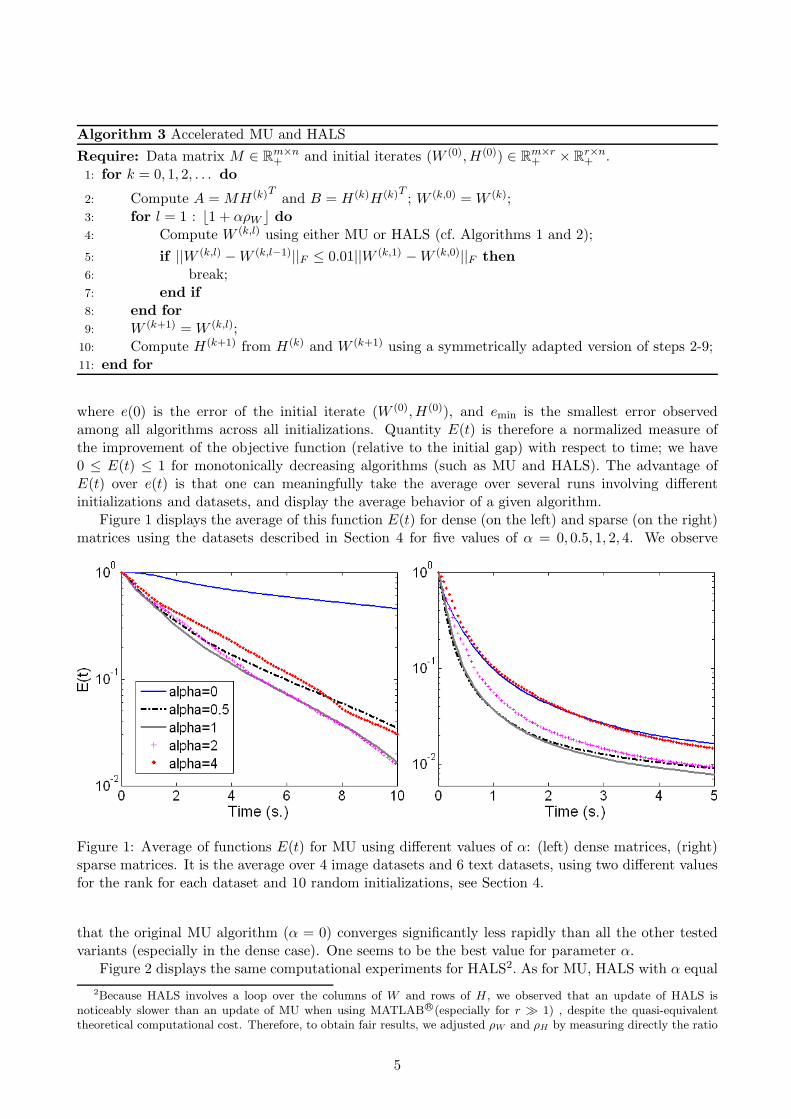
Figure 1 displays the average of this function E(t) for dense (on the left) and sparse (on the right)matrices using the datasets described in Section 4 for five values of α = 0, 0.5, 1, 2, 4. We observe
Figure 1: Average of functions E(t) for MU using different values of α: (left) dense matrices, (right)sparse matrices. It is the average over 4 image datasets and 6 text datasets, using two different valuesfor the rank for each dataset and 10 random initializations, see Section 4.
that the original MU algorithm (α = 0) converges significantly less rapidly than all the other testedvariants (especially in the dense case). One seems to be the best value for parameter α.
Figure 2 displays the same computational experiments for HALS2. As for MU, HALS with α equal
2Because HALS involves a loop over the columns of W and rows of H , we observed that an update of HALS isnoticeably slower than an update of MU when using MATLABR©(especially for r ≫ 1) , despite the quasi-equivalenttheoretical computational cost. Therefore, to obtain fair results, we adjusted ρW and ρH by measuring directly the ratio
5
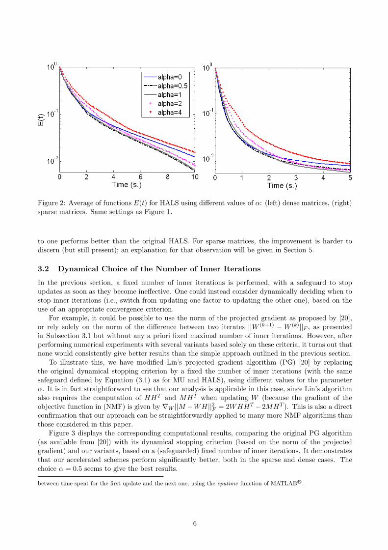
Figure 2: Average of functions E(t) for HALS using different values of α: (left) dense matrices, (right)sparse matrices. Same settings as Figure 1.
to one performs better than the original HALS. For sparse matrices, the improvement is harder todiscern (but still present); an explanation for that observation will be given in Section 5.
3.2 Dynamical Choice of the Number of Inner Iterations
In the previous section, a fixed number of inner iterations is performed, with a safeguard to stopupdates as soon as they become ineffective. One could instead consider dynamically deciding when tostop inner iterations (i.e., switch from updating one factor to updating the other one), based on theuse of an appropriate convergence criterion.
For example, it could be possible to use the norm of the projected gradient as proposed by [20],or rely solely on the norm of the difference between two iterates ||W (k+1) − W (k)||F , as presentedin Subsection 3.1 but without any a priori fixed maximal number of inner iterations. However, afterperforming numerical experiments with several variants based solely on these criteria, it turns out thatnone would consistently give better results than the simple approach outlined in the previous section.
To illustrate this, we have modified Lin’s projected gradient algorithm (PG) [20] by replacingthe original dynamical stopping criterion by a fixed the number of inner iterations (with the samesafeguard defined by Equation (3.1) as for MU and HALS), using different values for the parameterα. It is in fact straightforward to see that our analysis is applicable in this case, since Lin’s algorithmalso requires the computation of HHT and MHT when updating W (because the gradient of theobjective function in (NMF) is given by ∇W ||M −WH||2F = 2WHHT −2MHT ). This is also a directconfirmation that our approach can be straightforwardly applied to many more NMF algorithms thanthose considered in this paper.
Figure 3 displays the corresponding computational results, comparing the original PG algorithm(as available from [20]) with its dynamical stopping criterion (based on the norm of the projectedgradient) and our variants, based on a (safeguarded) fixed number of inner iterations. It demonstratesthat our accelerated schemes perform significantly better, both in the sparse and dense cases. Thechoice α = 0.5 seems to give the best results.
between time spent for the first update and the next one, using the cputime function of MATLABR©.
6
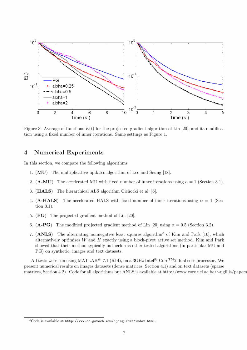
Figure 3: Average of functions E(t) for the projected gradient algorithm of Lin [20], and its modifica-tion using a fixed number of inner iterations. Same settings as Figure 1.
4 Numerical Experiments
In this section, we compare the following algorithms
1. (MU) The multiplicative updates algorithm of Lee and Seung [18].
2. (A-MU) The accelerated MU with fixed number of inner iterations using α = 1 (Section 3.1).
3. (HALS) The hierarchical ALS algorithm Cichocki et al. [6].
4. (A-HALS) The accelerated HALS with fixed number of inner iterations using α = 1 (Sec-tion 3.1).
5. (PG) The projected gradient method of Lin [20].
6. (A-PG) The modified projected gradient method of Lin [20] using α = 0.5 (Section 3.2).
7. (ANLS) The alternating nonnegative least squares algorithm3 of Kim and Park [16], whichalternatively optimizes W and H exactly using a block-pivot active set method. Kim and Parkshowed that their method typically outperforms other tested algorithms (in particular MU andPG) on synthetic, images and text datasets.
All tests were run using MATLABR© 7.1 (R14), on a 3GHz IntelR© CoreTM2 dual core processor. Wepresent numerical results on images datasets (dense matrices, Section 4.1) and on text datasets (sparsematrices, Section 4.2). Code for all algorithms but ANLS is available at http://www.core.ucl.ac.be/∼ngillis/papers/AccMUHALSPG.zip.
3Code is available at http://www.cc.gatech.edu/~jingu/nmf/index.html.
7
4.1 Dense Matrices - Images Datasets
Table 1 summarizes characteristics for the different datasets.
Table 1: Image datasets.Data # pixels m n r ⌊ρW ⌋ ⌊ρH⌋
ORL1 112 × 92 10304 400 30, 60 358, 195 13, 7Umist2 112 × 92 10304 575 30, 60 351, 188 19, 10CBCL3 19 × 19 361 2429 30, 60 12, 7 85, 47Frey2 28 × 20 560 1965 30, 60 19, 10 67, 36
⌊x⌋ denotes the largest integer smaller than x.1 http://www.cl.cam.ac.uk/research/dtg/attarchive/facedatabase.html2 http://www.cs.toronto.edu/~roweis/data.html3 http://cbcl.mit.edu/cbcl/software-datasets/FaceData2.html
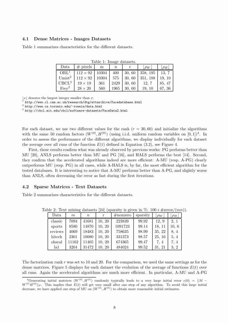
For each dataset, we use two different values for the rank (r = 30, 60) and initialize the algorithmswith the same 50 random factors (W (0),H(0)) (using i.i.d. uniform random variables on [0, 1])4. Inorder to assess the performance of the different algorithms, we display individually for each datasetthe average over all runs of the function E(t) defined in Equation (3.2), see Figure 4.
First, these results confirm what was already observed by previous works: PG performs better thanMU [20], ANLS performs better than MU and PG [16], and HALS performs the best [14]. Second,they confirm that the accelerated algorithms indeed are more efficient: A-MU (resp. A-PG) clearlyoutperforms MU (resp. PG) in all cases, while A-HALS is, by far, the most efficient algorithm for thetested databases. It is interesting to notice that A-MU performs better than A-PG, and slightly worsethan ANLS, often decreasing the error as fast during the first iterations.
4.2 Sparse Matrices - Text Datasets
Table 2 summarizes characteristics for the different datasets.
Table 2: Text mining datasets [24] (sparsity is given in %: 100 ∗ #zeros/(mn)).Data m n r #nonzero sparsity ⌊ρW ⌋ ⌊ρH⌋
classic 7094 41681 10, 20 223839 99.92 12, 9 2, 1sports 8580 14870 10, 20 1091723 99.14 18, 11 10, 6reviews 4069 18483 10, 20 758635 98.99 35, 22 8, 4hitech 2301 10080 10, 20 331373 98.57 25, 16 5, 4ohscal 11162 11465 10, 20 674365 99.47 7, 4 7, 4
la1 3204 31472 10, 20 484024 99.52 31, 21 3, 2
The factorization rank r was set to 10 and 20. For the comparison, we used the same settings as for thedense matrices. Figure 5 displays for each dataset the evolution of the average of functions E(t) overall runs. Again the accelerated algorithms are much more efficient. In particular, A-MU and A-PG
4Generating initial matrices (W (0), H(0)) randomly typically leads to a very large initial error e(0) = ||M −W (0)H(0)||F . This implies that E(t) will get very small after one step of any algorithm. To avoid this large initialdecrease, we have applied one step of MU on (W (0), H(0)) to obtain more reasonable initial estimates.
8
Figure 4: Average of functions E(t) for different image datasets: ORL (top left), Umist (top right),CBCL (bottom left) and Frey (bottom right).
converge initially much faster than ANLS, and also obtain better final solutions5. A-MU, HALS andA-HALS have the fastest initial convergence rate, and HALS and A-HALS generate the best solutionsin all cases. Notice that A-HALS does not always perform better than HALS, the reason being thatHALS already performs remarkably well and that values of ρW and ρH are typically much lower thanfor dense datasets. Another explanation for that behavior is given in the next section.
5We also observe that ANLS no longer outperforms the original MU and PG algorithms, and only sometimes generatebetter final solutions.
9
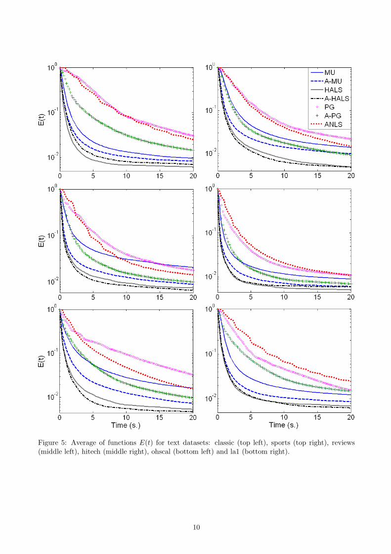
Figure 5: Average of functions E(t) for text datasets: classic (top left), sports (top right), reviews(middle left), hitech (middle right), ohscal (bottom left) and la1 (bottom right).
10
5 Why do HALS and A-HALS perform (so) well?
It is well-known that (block) coordinate-descent methods typically fail to converge rapidly becauseof their zig-zagging behavior, similar to what is frequently observed for gradient descent approaches,see, e.g., [2]. However, for the NNLS subproblems arising in NMF, we have observed in the previoussection that this approach (i.e., HALS and A-HALS) is quite efficient (see also [4, 14, 11, 19]). In thissection, we offer a theoretical explanation for that fact. This is based on two simple observations.
First, it is well-known that NMF solutions are typically parts-based: this is the main reason whyNMF has become so popular as a data analysis technique [17]. More precisely, any NMF decomposition(W,H) of M provides a linear model for the columns (resp. rows) of M with
M:j =
r∑
k=1
W:kHkj (resp. Mi: =
r∑
k=1
WikHi:),
where the columns of W (resp. the rows of H) are nonnegative basis elements, and each column of H(resp. each row of W ) contains the nonnegative weights of the linear combination approximating eachcolumn (resp. each row) of M . Because of these nonnegativity constraints on both the basis elementsand the weights, the factorization can be viewed as an additive reconstruction, and the columns of W(resp. the rows of H) typically represent different parts of the original data (e.g., for facial images,basis elements typically represent facial features such as eyes, noses and lips [17]). Therefore, supports(sets of nonzero entries) of the columns of W (resp. rows of H) typically share few elements. In otherwords, these supports are almost disjoint, implying that the matrix product W TW (resp. HHT ) haslarge entries on its diagonal, and zeros or small entries nearly everywhere else.
Second, the NNLS problem minW≥0 ||M −WH||2F can be decomposed into m independent NNLSsubproblems, corresponding to each row of W , since
||M − WH||2F =
m∑
i=1
||Mi: − Wi:H||2F .
Each of these NNLS subproblems can be formulated, for a given row Wi:, as follows:
minWi:≥0
||Mi: − Wi:H||2F = Wi:(HHT )W Ti: − 2Wi:HMT
i: + Mi:MTi: , 1 ≤ i ≤ m. (5.1)
The quadratic term Wi:(HHT )W Ti: is the only place where variables Wi: are coupled together (the
rest being separable), and depends on the (Hessian) matrix HHT . In particular, if HHT is diagonal,Problem (5.1) can be decoupled in r NNLS problems in one variable minWik≥0 ||Mi: − WikHk:||
2F , for
which an exact coordinate descent method would generate an optimal solution in one step (i.e., afterthe update of each variable). We therefore have the following result.
Theorem 1. Let M ∈ Rm×n+ and H ∈ R
m×r+ . If HHT is a diagonal matrix, which happens in
particular when supports of the rows of H are disjoint, then an optimal solution W ∗ to the NNLS
problem
minW≥0
||M − WH||2F , (NNLS)
can be obtained by performing one iteration of the exact coordinate descent method from any initial
matrix, i.e., by a single HALS update.
More generally, if matrix HHT is close to being diagonal, Problem (5.1) typically features largecoefficients for the quadratic terms (namely W 2
ik) in comparison to the bilinear terms (namely WikWip,k 6= p). Intuitively, this implies that the interaction between variables is low and therefore optimizingone variable at a time is still a relatively efficient procedure.
11
Combining the above two observations, we conclude that performing a few iterations of HALS onthe NNLS subproblems arising in NMF allows the algorithm to get close to an optimum solution. Thisis especially true for sparse matrices M , since factors (W,H) will be even sparser, which also gives anexplanation for the closer performance of HALS and its accelerated variant on sparse matrices.
6 Conclusion
In this paper, we considered the multiplicative updates [18] and the hierarchical alternating leastsquares algorithm [6] for nonnegative matrix factorization (NMF). We introduced accelerated variantsof these two schemes, based on a careful analysis of the computational cost they spend at each iteration.The idea behind our approach is based on taking better advantage of the most expensive part of thealgorithms, by repeating a fixed number of times the cheaper part of the iterations. This techniquecan in principle be applied to most NMF algorithms; in particular, we showed how it can improvethe projected gradient method from [20]. We then experimentally showed that these acceleratedvariants, despite the relative simplicity of the modification, significantly outperform the original ones,especially on dense matrices, and compete favorably with a state-of-the-art algorithm, namely theANLS method [16]. A direction for future research would be to choose the number of inner iterationsin a more sophisticated way, with the hope of further improving the efficiency of A-MU, A-PG andA-HALS.
Finally, we observed that HALS and its accelerated version are the most efficient variants forsolving NMF problems, sometimes by far. Besides our extensive numerical experiments, we haveprovided a theoretical explanation for that fact. The reason is that NMF solutions are expected tobe parts-based, meaning that in a decomposition M ≈ WH supports of the columns of W (resp. ofthe rows of H) will be ‘almost’ disjoint. This makes NNLS subproblems nearly separable, allowing anexact coordinate descent method such as HALS to solve them efficiently.
References
[1] M. Berry, M. Browne, A. Langville, P. Pauca, and R.J. Plemmons, Algorithms and Applications
for Approximate Nonnegative Matrix Factorization, Computational Statistics and Data Analysis, 52 (2007),pp. 155–173.
[2] D.P. Bertsekas, Nonlinear Programming: Second Edition, Athena Scientific, Massachusetts, 1999.
[3] A. Cichocki, S. Amari, R. Zdunek, and A.H. Phan, Non-negative Matrix and Tensor Factorizations:
Applications to Exploratory Multi-way Data Analysis and Blind Source Separation, Wiley-Blackwell, 2009.
[4] A. Cichocki and A-H. Phan, Fast local algorithms for large scale Nonnegative Matrix and Tensor
Factorizations, IEICE Transactions on Fundamentals of Electronics, Vol. E92-A No.3 (2009), pp. 708–721.
[5] A. Cichocki, R. Zdunek, and S. Amari, Non-negative Matrix Factorization with Quasi-Newton Opti-
mization, in Lecture Notes in Artificial Intelligence, Springer, vol. 4029, 2006, pp. 870–879.
[6] , Hierarchical ALS Algorithms for Nonnegative Matrix and 3D Tensor Factorization, Lecture Notesin Computer Science, Springer, 4666 (2007), pp. 169–176.
[7] M.E. Daube-Witherspoon and G. Muehllehner, An iterative image space reconstruction algorithm
suitable for volume ect, IEEE Trans. Med. Imaging, 5 (1986), pp. 61–66.
[8] K. Devarajan, Nonnegative Matrix Factorization: An Analytical and Interpretive Tool in Computational
Biology, PLoS Computational Biology, 4(7), e1000029 (2008).
[9] I.S. Dhillon, D. Kim, and S. Sra, Fast Newton-type Methods for the Least Squares Nonnegative Matrix
Approximation problem, in Proc. of SIAM Conf. on Data Mining, 2007.
[10] C. Ding, X. He, and H.D. Simon, On the Equivalence of Nonnegative Matrix Factorization and Spectral
Clustering, in SIAM Int’l Conf. Data Mining (SDM’05), 2005, pp. 606–610.
12
[11] N. Gillis and F. Glineur, Nonnegative Factorization and The Maximum Edge Biclique Problem. CORE
Discussion paper 2008/64, 2008.
[12] , Nonnegative Matrix Factorization and Underapproximation. Communication at 9th InternationalSymposium on Iterative Methods in Scientific Computing, Lille, France, 2008.
[13] J. Han, L. Han, M. Neumann, and U. Prasad, On the rate of convergence of the image space recon-
struction algorithm, Operators and Matrices, 3(1) (2009), pp. 41–58.
[14] N.-D. Ho, Nonnegative Matrix Factorization - Algorithms and Applications, PhD thesis, Universitecatholique de Louvain, 2008.
[15] H. Kim and H. Park, Non-negative Matrix Factorization Based on Alternating Non-negativity Con-
strained Least Squares and Active Set Method, SIAM J. Matrix Anal. Appl., 30(2) (2008), pp. 713–730.
[16] J. Kim and H. Park, Toward Faster Nonnegative Matrix Factorization: A New Algorithm and Compar-
isons, in Proceedings of IEEE International Conference on Data Mining, 2008, pp. 353–362.
[17] D.D. Lee and H.S. Seung, Learning the Parts of Objects by Nonnegative Matrix Factorization, Nature,401 (1999), pp. 788–791.
[18] , Algorithms for Non-negative Matrix Factorization, In Advances in Neural Information Processing,13 (2001).
[19] L. Li and Y.-J. Zhang, FastNMF: highly efficient monotonic fixed-point nonnegative matrix factorization
algorithm with good applicability, J. Electron. Imaging, Vol. 18 (033004) (2009).
[20] C.-J. Lin, Projected Gradient Methods for Nonnegative Matrix Factorization, Neural Computation, 19(2007), pp. 2756–2779. MIT press.
[21] P. Pauca, J. Piper, and R. Plemmons, Nonnegative matrix factorization for spectral data analysis,Linear Algebra and its Applications, 406(1) (2006), pp. 29–47.
[22] F. Shahnaz, M.W. Berry, A. Langville, V.P. Pauca, and R.J. Plemmons, Document clustering
using nonnegative matrix factorization, Information Processing and Management, 42 (2006), pp. 373–386.
[23] S.A. Vavasis, On the complexity of nonnegative matrix factorization, SIAM Journal on Optimization,20(3) (2009), pp. 1364–1377.
[24] S. Zhong and J. Ghosh, Generative model-based document clustering: a comparative study, Knowledgeand Information Systems, 8 (3) (2005), pp. 374–384.
13
Recent titles CORE Discussion Papers
2010/76. Ana MAULEON, Vincent VANNETELBOSCH and Cecilia VERGARI. Unions' relative
concerns and strikes in wage bargaining. 2010/77. Ana MAULEON, Vincent VANNETELBOSCH and Cecilia VERGARI. Bargaining and delay
in patent licensing. 2010/78. Jean J. GABSZEWICZ and Ornella TAROLA. Product innovation and market acquisition of
firms. 2010/79. Michel LE BRETON, Juan D. MORENO-TERNERO, Alexei SAVVATEEV and Shlomo
WEBER. Stability and fairness in models with a multiple membership. 2010/80. Juan D. MORENO-TERNERO. Voting over piece-wise linear tax methods. 2010/81. Jean HINDRIKS, Marijn VERSCHELDE, Glenn RAYP and Koen SCHOORS. School
tracking, social segregation and educational opportunity: evidence from Belgium. 2010/82. Jean HINDRIKS, Marijn VERSCHELDE, Glenn RAYP and Koen SCHOORS. School
autonomy and educational performance: within-country evidence. 2010/83. Dunia LOPEZ-PINTADO. Influence networks. 2010/84. Per AGRELL and Axel GAUTIER. A theory of soft capture. 2010/85. Per AGRELL and Roman KASPERZEC. Dynamic joint investments in supply chains under
information asymmetry. 2010/86. Thierry BRECHET and Pierre M. PICARD. The economics of airport noise: how to manage
markets for noise licenses. 2010/87. Eve RAMAEKERS. Fair allocation of indivisible goods among two agents. 2011/1. Yu. NESTEROV. Random gradient-free minimization of convex functions. 2011/2. Olivier DEVOLDER, François GLINEUR and Yu. NESTEROV. First-order methods of
smooth convex optimization with inexact oracle. 2011/3. Luc BAUWENS, Gary KOOP, Dimitris KOROBILIS and Jeroen V.K. ROMBOUTS. A
comparison of forecasting procedures for macroeconomic series: the contribution of structural break models.
2011/4. Taoufik BOUEZMARNI and Sébastien VAN BELLEGEM. Nonparametric Beta kernel estimator for long memory time series.
2011/5. Filippo L. CALCIANO. The complementarity foundations of industrial organization. 2011/6. Vincent BODART, Bertrand CANDELON and Jean-François CARPANTIER. Real exchanges
rates in commodity producing countries: a reappraisal. 2011/7. Georg KIRCHSTEIGER, Marco MANTOVANI, Ana MAULEON and Vincent
VANNETELBOSCH. Myopic or farsighted? An experiment on network formation. 2011/8. Florian MAYNERIS and Sandra PONCET. Export performance of Chinese domestic firms: the
role of foreign export spillovers. 2011/9. Hiroshi UNO. Nested potentials and robust equilibria. 2011/10. Evgeny ZHELOBODKO, Sergey KOKOVIN, Mathieu PARENTI and Jacques-François
THISSE. Monopolistic competition in general equilibrium: beyond the CES. 2011/11. Luc BAUWENS, Christian HAFNER and Diane PIERRET. Multivariate volatility modeling of
electricity futures. 2011/12. Jacques-François THISSE. Geographical economics: a historical perspective. 2011/13. Luc BAUWENS, Arnaud DUFAYS and Jeroen V.K. ROMBOUTS. Marginal likelihood for
Markov-switching and change-point GARCH models. 2011/14. Gilles GRANDJEAN. Risk-sharing networks and farsighted stability. 2011/15. Pedro CANTOS-SANCHEZ, Rafael MONER-COLONQUES, José J. SEMPERE-MONERRIS
and Oscar ALVAREZ-SANJAIME. Vertical integration and exclusivities in maritime freight transport.
2011/16. Géraldine STRACK, Bernard FORTZ, Fouad RIANE and Mathieu VAN VYVE. Comparison of heuristic procedures for an integrated model for production and distribution planning in an environment of shared resources.
Recent titles CORE Discussion Papers - continued
2011/17. Juan A. MAÑEZ, Rafael MONER-COLONQUES, José J. SEMPERE-MONERRIS and
Amparo URBANO Price differentials among brands in retail distribution: product quality and service quality.
2011/18. Pierre M. PICARD and Bruno VAN POTTELSBERGHE DE LA POTTERIE. Patent office governance and patent system quality.
2011/19. Emmanuelle AURIOL and Pierre M. PICARD. A theory of BOT concession contracts. 2011/20. Fred SCHROYEN. Attitudes towards income risk in the presence of quantity constraints. 2011/21. Dimitris KOROBILIS. Hierarchical shrinkage priors for dynamic regressions with many
predictors. 2011/22. Dimitris KOROBILIS. VAR forecasting using Bayesian variable selection. 2011/23. Marc FLEURBAEY and Stéphane ZUBER. Inequality aversion and separability in social risk
evaluation. 2011/24. Helmuth CREMER and Pierre PESTIEAU. Social long term care insurance and redistribution. 2011/25. Natali HRITONENKO and Yuri YATSENKO. Sustainable growth and modernization under
environmental hazard and adaptation. 2011/26. Marc FLEURBAEY and Erik SCHOKKAERT. Equity in health and health care. 2011/27. David DE LA CROIX and Axel GOSSERIES. The natalist bias of pollution control. 2011/28. Olivier DURAND-LASSERVE, Axel PIERRU and Yves SMEERS. Effects of the uncertainty
about global economic recovery on energy transition and CO2 price. 2011/29. Ana MAULEON, Elena MOLIS and Vincent J. VANNETELBOSCH. Absolutely stable
roommate problems. 2011/30. Nicolas GILLIS and François GLINEUR. Accelerated multiplicative updates and hierarchical
als algorithms for nonnegative matrix factorization.
Books P. VAN HENTENRYCKE and L. WOLSEY (eds.) (2007), Integration of AI and OR techniques in constraint
programming for combinatorial optimization problems. Berlin, Springer. P-P. COMBES, Th. MAYER and J-F. THISSE (eds.) (2008), Economic geography: the integration of
regions and nations. Princeton, Princeton University Press. J. HINDRIKS (ed.) (2008), Au-delà de Copernic: de la confusion au consensus ? Brussels, Academic and
Scientific Publishers. J-M. HURIOT and J-F. THISSE (eds) (2009), Economics of cities. Cambridge, Cambridge University Press. P. BELLEFLAMME and M. PEITZ (eds) (2010), Industrial organization: markets and strategies. Cambridge
University Press. M. JUNGER, Th. LIEBLING, D. NADDEF, G. NEMHAUSER, W. PULLEYBLANK, G. REINELT, G.
RINALDI and L. WOLSEY (eds) (2010), 50 years of integer programming, 1958-2008: from the early years to the state-of-the-art. Berlin Springer.
G. DURANTON, Ph. MARTIN, Th. MAYER and F. MAYNERIS (eds) (2010), The economics of clusters – Lessons from the French experience. Oxford University Press.
J. HINDRIKS and I. VAN DE CLOOT (eds) (2011), Notre pension en heritage. Itinera Institute.
CORE Lecture Series D. BIENSTOCK (2001), Potential function methods for approximately solving linear programming
problems: theory and practice. R. AMIR (2002), Supermodularity and complementarity in economics. R. WEISMANTEL (2006), Lectures on mixed nonlinear programming.