Embed Size (px)
Citation preview
Technical Paper 10 June 1980 Change 3
DDESB
Methodology for
Chemical Hazard Prediction
Department of Defense Explosives Safety Board
Alexandria, Virginia

This page intentionally left blank

DDESB TP 10, Change 3, June 1980
i
PREFACE
This document describes an atmospheric-diffusion model which provides an appropriate
method for calculating hazard-distances associated with chemical accidents or incidents for
emergency-planning purposes. Background, experience, and judgment are required in the
responsible employment of these methods. That judgment is required to determine source
parameters, to use the meteorological input parameters, and to apply the model to situations
involving changing meteorological environments. Integrity of the results obtained will reflect
the users’ understanding of the physical processes, models, methods and, when utilized,
computer programs.
The method described in this Technical Paper is the product of a coordinated effort of
Technical Advisors to the Chemical Standards Working Group, DoD Explosives Safety Board.
The Technical Advisors were Mr. P. E. Carlson (Dugway Proving Ground), Mr. C. G. Whitacre
(Chemical Systems Laboratory, US Army Armament Research and Development Command),
Mr. J. D. Wood (US Army Ordnance and Chemical Center and School), Mr. I. Solomon
(retired), and Mr. M. C. Johnson (US Army Armament Materiel Readiness Command). In
addition, considerable expert advice and support in matters related to meteorology were provided
by Dr. H. E. Cramer of H. E. Cramer Company under DPG Contract DAAD09-74-C-0005.
The original Working Group members were:
Dr. R. A. Scott, Jr., DDESB, Chairman
Mr. J. M. Hawes, US Army Materiel Development and Readiness Command
Mr. D. F. Abernethy, HQDA, Office of the Inspector General
Mr. F. B. Sanchez, NSWC, Dahlgren, VA
Mr. R. Alg, AF Inspection & Safety Center, Norton AFB, CA
The concerted effort exerted by the above named persons is appreciated. It is considered to
be a significant advance in the evaluation of the downwind hazards associated with the release of
toxic chemical materials.
Change 3 incorporates methodology for agent evaporation in still air. The technical
assistance of Headquarters, US Army Armament Materiel Readiness Command in reviewing this
change is acknowledged and greatly appreciated.
ALTON W. POWELL
Colonel, USAF
Chairman
June 1980
This Change 3 supersedes the original publication and subsequent changes which should be
destroyed.

This page intentionally left blank

DDESB TP 10, Change 3, June 1980
Table of Contents
TABLE OF CONTENTS
PREFACE ........................................................................................................................................ i
CHAPTER 1. INTRODUCTION ...................................................................................................1
1.1. Purpose ...............................................................................................................................1
1.2. Scope ..................................................................................................................................1
CHAPTER 2. THE RECOMMENDED MODEL ..........................................................................2
2.1. General ...............................................................................................................................2
2.2. The Basic Model ................................................................................................................2
2.3. A Generalized Model .........................................................................................................4
CHAPTER 3. SPECIAL CONSIDERATIONS .............................................................................5
3.1. General ...............................................................................................................................5
3.2. Stability Change Criteria....................................................................................................5
3.3. Personnel Exposure Times .................................................................................................6
3.4. Evaporation from Liquid Spills .........................................................................................7
3.5. Rise of Heated Plumes .......................................................................................................7
3.5.1. General ......................................................................................................................7
3.5.2. Instantaneous Releases in Stable Atmospheres ......................................................14
3.5.3. Quasi-Continuous Releases in Stable Atmospheres ...............................................14
CHAPTER 4. SUPPORTING DATA ..........................................................................................16
4.1. General .............................................................................................................................16
4.2. Meteorological Parameters ..............................................................................................16
4.3. Toxicity ............................................................................................................................18
SUMMARY ...................................................................................................................................20
REFERENCES ..............................................................................................................................21
ANNEXES
ANNEX A – THE GENERALIZED PREDICTION MODEL ...............................................22
ANNEX B – TOXICITY FOR GB AND VX AS A FUNCTION OF EXPOSURE TIME ...37
ANNEX C – METHOD FOR CALCULATING RATES OF EVAPORATION FROM
PUDDLES OF LIQUID TOXIC SUBSTANCES .............................................................45
ANNEX D – METHODS FOR CALCULATING HAZARDS FOR EXPLOSIVE
DISSEMINATION OF VX AND HD ...............................................................................53

DDESB TP 10, Change 3, June 1980
Table of Contents
DD FORM 1473 ............................................................................................................................61
DISTRIBUTION LIST ..................................................................................................................62
TABLES
TABLE 1. KEY TO STABILITY CATEGORIES ................................................................16
TABLE 2. RECOMMENDED VALUES OF PARAMETERS (OPEN TERRAIN).............17
TABLE 3. RECOMMENDED VALUES OF PARAMETERS (FORESTED TERRAIN) ...17
TABLE 4. TOXICITY VALUES (mg-min/m3) .....................................................................18
FIGURES
FIGURE 1. EVAPORATION RATES FOR LIQUID SPILLS OF GB WITH VARIOUS
WIND SPEEDS AND AIR TEMPERATURES .................................................................8
FIGURE 2. EVAPORATION RATES FOR LIQUID SPILLS OF GB IN STILL AIR
WITH A VARIETY OF AIR TEMPERATURES ..............................................................9
FIGURE 3. EVAPORATION RATES FOR LIQUID SPILLS OF VX WITH VARIOUS
WIND SPEEDS AND AIR TEMPERATURES ...............................................................10
FIGURE 4. EVAPORATION RATES FOR LIQUID SPILLS OF VX IN STILL AIR
WITH A VARIETY OF AIR TEMPERATURES ............................................................11
FIGURE 5. EVAPORATION RATES FOR LIQUID SPILLS OF HD WITH VARIOUS
WIND SPEEDS AND AIR TEMPERATURES ...............................................................12
FIGURE 6. EVAPORATION RATES FOR LIQUID SPILLS OF HD IN STILL AIR
WITH A VARIETY OF AIR TEMPERATURES ............................................................13
FIGURE D.1. HAZARD DISTANCE FOR EXPLOSIVELY DISSEMINATED VX .........57
FIGURE D.2. NOMOGRAPH FOR DETERMINATION OF THE FINAL REFERENCE
VALUE FOR AGENT HD ................................................................................................59

This page intentionally left blank

DDESB TP 10, Change 3, June 1980
Chapter 1: Introduction 1
CHAPTER 1
INTRODUCTION
1.1. PURPOSE. The purpose of the Technical Paper is to present a description of the current,
recommended method for estimating chemical hazard distances for planning purposes.
1.2. SCOPE
This Technical Paper describes an appropriate method for estimating, for planning purposes,
hazard distances associated with hypothetical Maximum Credible Events (MCE) from which
toxic substances might be released into the atmosphere. In particular, the method comprises a
mathematical model, which reflects the current state-of-the-art in atmospheric diffusion
modeling, and complete sets of input data representing appropriate parametric values for wide
ranges of geographical and meteorological environments. Certain subordinate mathematical
models are also provided to facilitate calculations when the MCE includes either spills of toxic
substances onto ground surfaces or plumes which ascend rapidly because of heat generated by
fuel fires, etc.
Not included in the scope of this Technical Paper are those factors which lead to
development and identification of the MCE.

This page intentionally left blank

Chapter 2: The Recommended Model 2
CHAPTER 2
THE RECOMMENDED MODEL
2.1. GENERAL
a. The recommended method for calculating toxic vapor hazard distances for planning
purposes, given the agent source configurations, is a Gaussian Plume diffusion model with (a)
provisions for limiting the vertical expansion of the cloud to the surface mixing layer and (b)
criteria to accommodate time-space variations of meteorological and other environmental
factors. The theoretical basis for that model has been extensively investigated and reported by
Sutton1*
and Pasquill2, among others. Sutton shows that the Gaussian Plume model is a natural
consequence of treating atmospheric diffusion as an analogy to molecular diffusion. Diffusion
coefficients associated with Brownian motion in the molecular case are simply replaced by those
associated with the size of thermally-generated wind eddies in the atmospheric case.
b. Historically, the practical problem has been to determine the rate of diffusion from
observations of plume densities (concentrations) and simultaneous measurements of purely
meteorological entities, such as wind, temperature, cloud cover and relative humidity. Even, in
the simplest case, i.e., flat, level and open terrain free from vegetation and man-made structures,
the problem is not an easy one. The presence of hills, vegetation and structures further
complicates the practical problem.
A majority of toxic vapor hazard problems can be treated adequately with the Basic Model
described below. It is applicable when the ground-level, axial, total dosage is required in an
idealized topographic situation (i.e., flat, level and open terrain). Problems which do not fall in
this category can be treated via either the more general or more special methods described in the
various Annexes to this Technical Paper.
2.2. THE BASIC MODEL
The basic equation for computing the axial dosage at ground level from an elevated,
instantaneous, point-source or computing axial concentration at ground level from an elevated,
continuous, point-source is:
________________________
* Superscript numerals designate references listed at the end of text.

Chapter 2: The Recommended Model 3
where:
D = the axial dosage in mg-min/cu m at a point, x, downwind (concentration in mg/cu m for
continuous point sources.
Q = the source strength in milligrams (milligrams/min for continuous sources).
σy & σz = the standard deviations of crosswind and vertical concentrations respectively, in
meters. Both are functions of the distance, x.
Ux = the average speed of the cloud as it passes the point x, in meters/min.
Hm = the depth of the surface mixing layer, in meters.
H = the effective height of the source, in meters. (H should not exceed Hm in the above
equation).
Equation 2.1 can be approximated by a very simple linear expression,
at moderate distances, x, downwind from the toxic source, where the effect of the release height,
H, on the dosage, D(x), becomes negligible. At those distances, the toxic substance becomes
rather uniformly distributed in the vertical because of multiple reflections of material from the
assumed perfectly-reflecting planes at ground level and at the inversion cap height, Hm.
Equation 2.2. is commonly known as the “Box Model.” Because of its simplicity, it is preferred
over the more complex Equation 2.1. However, in practice, care must be taken to insure that
assumptions fundamental to the Basic Model remain valid (see paragraph 3.2, Stability Change
Criteria).
The parameters σy and σz, as used in the Basic Model, are defined as simple power-law
functions of the distance traveled by the toxic plume. Values for those parameters at any
downwind distance, x, are computed from auxiliary equations, as follows:

Chapter 2: The Recommended Model 4
where σyr and σzr are reference values at the distances xyr and xzr, respectively. Further, 𝛼 and 𝛽
are stability-dependent values which describe the expansion rates of the cloud laterally and
vertically, respectively. B and C are virtual distances calculated to allow for a volume source
and are obtained as follows:
Where σyR and σzR are the initial values describing the initial size of the toxic plume at the site of
the hypothetical accident/incident. Specification of values for the parameters σyR and σzR
requires a detailed knowledge of the source configuration in terms of toxic substance and its
physical state), source strength (Q), time duration of release, and height of the toxic plume’s
centroid. These elements of the source configuration must necessarily be derived from the
hypothetical MCE. They often involve complex technical judgements which are specific to the
MCE under study and which will be provided by the agency which conducts the scenario-
specific hazard study.
Recommended values for all meteorological variables introduced in the Basic Method have
been tabulated. They appear in paragraph 4.2. If, however, calculations are being made for a
location for which specific meteorological data are available, those data should be used in lieu of
the data in paragraph 4.2.
2.3. A GENERALIZED MODEL. The mathematical formulation of a generalized model is
presented in Annex A. The generalized model provides for variations in the composition and
quantity of the material released, as well as for variations in source dimensions, source height,
source emission time, and decay. Specific provision is also made in the generalized model for
the effects of gravitational settling and for computing dosages and concentrations for locations
other than downwind plume centerlines, at ground level. That model will also accommodate the
restriction of lateral diffusion due to orographic influences of terrain channeling. Meteorological
model inputs include mean wind speed, depth of the surface mixing layer, intensities of
turbulence, and vertical shear (i.e., wind direction and wind speed) in the mixing layer. Thus, the
generalized model contains both mesoscale and microscale meteorological predictors that may
be tailored to specific geographical locations and specific meteorological conditions.

This page intentionally left blank

DDESB TP 10, Change 3, June 1980
Chapter 3: Special Considerations 5
CHAPTER 3
SPECIAL CONSIDERATIONS
3.1. GENERAL. Four special considerations have been identified as necessary, on occasion, in
the application of the Basic Method to toxic hazard predictions. These are (1) stability-change
criteria, (2) personnel exposure times, (3) the rates of evaporation from spill s of toxic
substances, and (4) the extent of vertical rise of heated plumes which are generated by the heat
released from fuel fires, etc.
3.2. STABILITY CHANGE CRITERIA
The recommended Basic Model, and its implementation in terms of formulas given above,
computer programs, and parameter values shown in paragraph 4, is based on the assumption that
steady-state conditions exist throughout the air volume swept out by the toxic plume during its
lifetime. That volume might exceed billions of cubic meters (i.e., during its lifetime, the plume
might occupy air volumes whose dimensions are several kilometers in the vertical and lateral,
and hundreds of kilometers extending downwind from the plume’s source). Lifetimes of large,
dense plumes could reach tens or hundreds of hours. In many instances, the assumption that
steady-state conditions exist over those volumes and those time intervals simply fails: Even if
surface properties of the local terrain are uniform enough, over large land areas, to suggest
steady-state atmospheres, the normal diurnal changes would preclude maintenance of the steady-
state after several hours have elapsed. This situation typically occurs when large amounts of
toxic material are released during a very stable nighttime regime with very low wind speeds and
mixing depths. The maximum time-duration of a stable nighttime regime is generally 12 hours
or less, depending on the season of the year and the latitude.
Techniques have been developed to accommodate these dynamics within the current,
recommended Basic Model. The concept is as follows: Although it is recognized that transitions
in the atmospheric structure occur smoothly, they are treated as a series of discrete step-changes.
The computer-assisted calculations are interrupted at “appropriate” points in the process, final
calculated values of the plume variables recorded, and these final values are treated as initial
values in the next subsequent phase of the calculation. The “appropriate”" points in the process
are where the analyst has reason to believe that the atmospheric structure would have changed
enough to warrant its approximation as a discreet step-change. Thus, some judgement is
required.
In the case of the stable nighttime regime cited above, the step-change procedure would be to
progressively change the meteorological parameters, which represent the stability categories,
from stable to less stable, permitting a reasonable time of dwell in each category. During each
phase of the calculations, the axial dosages at downwind distances would be calculated via the
Box Model (Equation 2.2), where:

DDESB TP 10, Change 3, June 1980
Chapter 3: Special Considerations 6
Hmc = the depth of the surface inversion layer at the beginning of the change (m).
xc = location of the plume’s centroid at the beginning of the change (m).
σyr & xyr = the reference sigma and reference distance in the new stability category (m).
ΔHm = change in Hm over the interval (m)
Δt = time interval of change (min).
U & 𝛼 = new meteorological parameters.
σyc = the lateral sigma at the beginning of the change interval.
Where accuracy demands it, and where available resources and technical data input accuracies
permit it, the number of discrete steps used to simulate a gradual change in atmospheric
conditions could be increased to improve the validity of the approximation. Thus, these
techniques can account for the effects of changes in atmospheric stability on the concentration,
dosages and deposition patterns of toxic plumes. Normal procedures are used to calculate 1% casualty estimates from that information.
3.3. PERSONNEL EXPOSURE TIMES. Special methods can be used when specific
elements of the hazard analysis require consideration of the time interval during which personnel
might be exposed to airborne chemical agents. Those situations normally arise when personnel
are assumed to be exposed to very low concentrations of agent over extended periods of time
such that detoxification of agent occurs within their bodies. Under those circumstances, the
Basic Model would yield overestimates of hazard distances. However, appropriate modifications
have been made to the Basic Model to adapt it for use in those instances. The resultant,
recommended model, an extension of the Basic Model, is described in Annex B.

DDESB TP 10, Change 3, June 1980
Chapter 3: Special Considerations 7
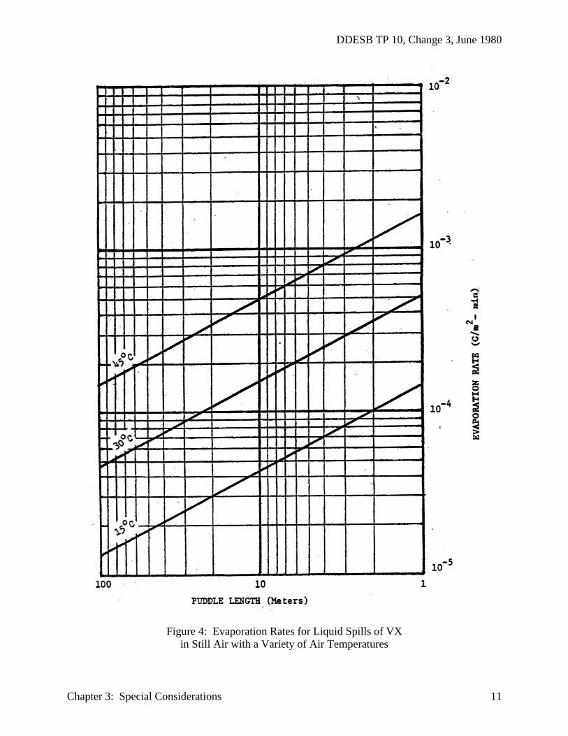
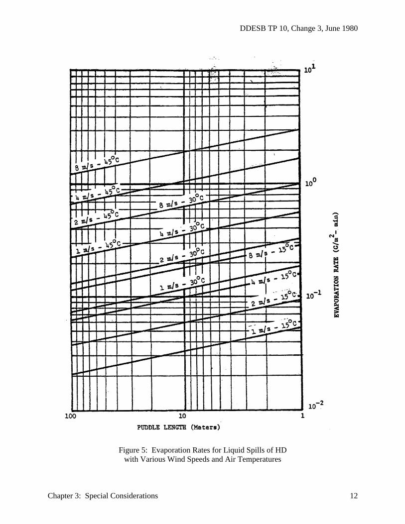
3.4. EVAPORATION FROM LIQUID SPILLS
Some MCE’s provide for spills of toxic materials onto ground surfaces. Toxic vapor plumes
are formed when the spilled material evaporates from those surfaces. Evaporation begins when
the toxic material is spilled, and it is assumed to continue until the toxic “puddle” has been
covered, decontaminated, or until all toxic material has evaporated. The plume, thus formed, is
assumed to have been generated from a “continuous source” of toxic material.
The Basic Model for toxic hazard estimation can be applied to the MCE for liquid spills by
the proper selection of parameter values: D(x) in Equation 2.1 is interpreted as concentration of
toxic substance in the plume, 3σyr is assumed equal to the width of the puddle, and Q is
interpreted as the rate of generation of toxic vapors (i.e., rate of evaporation of the toxic
substance from the puddle). In order to provide a basis for estimating evaporation rates from a
continum of puddle sizes and a variety of wind speed (to include still air), and air temperature
combinations, six graphs are presented in Figures 1 through 6 for GB, VX and HD, respectively.
In the event that the MCE involves toxic substances other than these three common chemical
warfare agents, or the required values are out of the range of values provided by these graphs, the
general methods for calculating evaporation rates under either a variety of wind speeds or in still
air can be used as indicated in Annex C.
3.5. RISE OF HEATED PLUMES
3.5.1. General
Toxic substances released in association with a fire or an explosion will usually rise as a
heated plume which entrains air until an equilibrium with ambient conditions is reached. Thus,
the effective source height, H, will be equal to the height attained as a result of buoyant rise zm.
The formulas given in this section, for instantaneous sources (explosions) and quasi-
continuous sources (fires or multiple explosions), are based on procedures similar to those
contained in a paper presented by Briggs (1970) at the Second International Clean Air Congress.3
Briggs’ equations differ in form for stable and adiabatic or unstable conditions. The form
proposed for adiabatic or unstable conditions contains the time of plume rise as an input value.
Since observed values of this parameter are not presently available, practical use of the
methodology is limited to the relation proposed for the stable atmosphere, for which this
parameter is not required. The equation is stated as a function of the vertical potential
temperature gradient and, thus, can be applied from stable to adiabatic.

DDESB TP 10, Change 3, June 1980
Chapter 3: Special Considerations 8
Figure 1: Evaporation Rates for Liquid Spills of GB
with Various Wind Speeds and Air Temperatures

DDESB TP 10, Change 3, June 1980
Chapter 3: Special Considerations 9
Figure 2: Evaporation Rates for Liquid Spills of GB
in Still Air with a Variety of Air Temperatures

DDESB TP 10, Change 3, June 1980
Chapter 3: Special Considerations 10
Figure 3: Evaporation Rates for Liquid Spills of VX
with Various Wind Speeds and Air Temperatures
DDESB TP 10, Change 3, June 1980
Chapter 3: Special Considerations 11
Figure 4: Evaporation Rates for Liquid Spills of VX
in Still Air with a Variety of Air Temperatures
DDESB TP 10, Change 3, June 1980
Chapter 3: Special Considerations 12
Figure 5: Evaporation Rates for Liquid Spills of HD
with Various Wind Speeds and Air Temperatures

DDESB TP 10, Change 3, June 1980
Chapter 3: Special Considerations 13
Figure 6: Evaporation Rates for Liquid Spills of HD
in Still Air with a Variety of Air Temperatures

DDESB TP 10, Change 3, June 1980
Chapter 3: Special Considerations 14
3.5.2. Instantaneous Releases in Stable Atmospheres
The maximum plume rise zmL downwind from an instantaneous source in a stable
atmosphere is given by:
An analysis of time-sequence photographs of the behavior of the ground plumes generated
during launches of the Titan I11 D vehicle at Vandenberg Air Force Base4 suggests that the value
of the instantaneous entrainment coefficient, YI, may range from about 0.5 to 0.7.
3.5.3. Quasi-Continuous Releases in Stable Atmospheres. The maximum plume rise zmc
downwind from a quasi-continuous source in a stable atmosphere is given by:

DDESB TP 10, Change 3, June 1980
Chapter 3: Special Considerations 15
Plume rise for launches of liquid-fueled rockets and for static firings suggests that the
entrainment coefficient γc is approximately equal to 0.5.

This page intentionally left blank

DDESB TP 10, Change 3, June 1980
Chapter 4: Supporting Data 16
CHAPTER 4
SUPPORTING DATA
4.1. GENERAL. Two types of supporting data are required in the application of the models to
the prediction of hazard distances from chemical accidents/incidents. These data are related to
the choices of meteorological parameters and toxicity data to be used in the calculations. Tables
of recommended meteorological parameters, together with some justification for their selection,
are presented in paragraph 4.2. Recommended values for toxicity of chemical agents at the “1%
lethality” for lethal agents and “l% incapacitation” for incapacitating agents are presented in
paragraph 4.3.
4.2. METEOROLOGICAL PARAMETERS
Meteorological inputs required for use in the Basic Model are listed below. The specification
of numerical values for the meteorological inputs requires, in principle, a complete knowledge of
the atmospheric structure of the air volume in which the plume is transported. Because of the
large distance scales and the large air volume that may be swept out by toxic plumes, the
measurement and specification of representative meteorological inputs is difficult. Thus, it is
usually necessary to estimate the requisite meteorological parameters, for any given location,
from historical surface meteorological observations, using various approximate techniques based
on theory and previous measurements. That has been done for the eleven Army storage depots
where chemical material is stored. Those data are presented in Appendix D of the “Handbook
for Chemical Hazard Prediction”.5
To facilitate hazard distance calculations, the required parameters have been presented for
each class of the Pasquill stability categories. The six categories are denoted by the letters A
through E. Categories A, B and C represent decreasing degrees of instability; E and F represent
increasing degrees of stability; and D is neutral. A summary table relating the stability
categories to atmospheric observeables, i.e., solar radiation and wind speed, is presented as Table
1; it has been adapted from Pasquill.2
TABLE 1. KEY TO STABILITY CATEGORIES
SURFACE WIND SPEED
(at 10m), m sec-1
DAY NIGHT
INCOMING SOLAR RADIATION CLOUD COVER
STRONG MODERATE SLIGHT >4/8 ≤3/8
<2 A A-B B
2-3 A-B B C E F
3-5 B B-C C D E
5-6 C C-D D D D
>6 C D D D D
Table 2 contains the required parameter values for flat, level and open terrain. Note that
reference σy values, σyr, are given for both a continuous and an instantaneous source: continuous

DDESB TP 10, Change 3, June 1980
Chapter 4: Supporting Data 17
refers to emission times on the order of 10 minutes or more, while instantaneous represents
emission times less than two and one-half seconds.
TABLE 2. RECOMMENDED VALUES OF PARAMETERS
(OPEN TERRAIN)
(xzr = xyr = 100 meters)
Pasquill
Stability
Category
σyr (Contin)
meters
σyr (Inst)
meters
α
σzr
meters
β
Hm
meters
A 27.0 9.00 1.0 14.0 1.40 2750
B 19.0 6.33 1.0 11.0 1.00 2250
C 12.5 4.80 1.0 7.5 0.90 1750
D 8.0 4.00 0.9 4.5 0.85 875
E 6.0 3.00 0.8 3.5 0.80 125
F 4.0 2.00 0.7 2.5 0.75 30
Within wooded or forested areas, the Pasquill stability categories, and their associated
meteorological parameter values, do not apply. Empirical data show that plumes under
forest/jungle canopies tend to expand to much larger volumes, at shorter travel distances, than do
those on flat, level and open terrain. Thus, the parameter values presented in Table 2 are not
representative of forested environments. Empirical data also show that wind speeds under
canopies are much lower than wind speeds external to the canopies at any given time. Thus,
plumes travel much farther over flat, level and open terrain than they do in forests, under any
given meteorological situation, in a given time. As a result, actual and predicted hazard
distances could be markedly different for open versus forested terrains. Table 3 presents a set of
meteorological parameter values for use in estimating hazard distances in forested environments.
These empirically-based data were derived by members of the former US Army MUCOM
Operations Research Group, from a variety of test data sources, only a few of which are
referenced here.6, 7, 8, 9
TABLE 3. RECOMMENDED VALUES OF PARAMETERS
(FORESTED TERRAIN)
(xyr = 100 meters, xzr = 20 meters)
REFERENCE
WIND SPEED
(mph)
OUTSIDE CANOPY
TRANSPORT
WIND SPEED,
U (mph)
UNDER CANOPY
σy α σz β
Deciduous Forest, Winter
1 0.2 12.8 0.80 1.3 1.20
5 1.0 12.1 1.00 1.4 1.20
12 2.4 12.0 1.00 1.5 1.20
20 4.0 12.0 1.10 1.5 1.20

DDESB TP 10, Change 3, June 1980
Chapter 4: Supporting Data 18
TABLE 3. RECOMMENDED VALUES OF PARAMETERS, CONTINUED
(FORESTED TERRAIN)
(xyr = 100 meters, xzr = 20 meters)
REFERENCE
WIND SPEED
(mph)
OUTSIDE CANOPY
TRANSPORT
WIND SPEED,
U (mph)
UNDER CANOPY
σy α σz β
Mixed Deciduous and Coniferous Forest, Winter
1 0.2 18.2 0.80 1.6 1.30
5 0.8 17.5 1.00 1.7 1.30
12 1.8 16.8 1.00 1.7 1.30
20 3.0 14.5 1.00 1.7 1.30
Coniferous Forest
1 0.2 23.5 0.80 1.8 1.30
5 0.8 22.5 1.00 1.9 1.30
12 1.8 19.0 1.00 1.9 1.30
20 3.0 14.0 1.00 1.9 1.30
Mixed Deciduous and Coniferous Forest, Summer
and Deciduous Forest, Summer
1 0.1 29.0 0.80 2.1 1.40
5 0.5 26.5 1.00 2.1 1.40
12 1.2 22.5 1.00 2.1 1.40
20 2.0 16.5 1.00 2.1 1.40
Tropical Rain Forest
1 0.1 53.0 1.00 6.9 1.00
5 0.3 36.0 1.00 6.9 1.00
12 0.6 26.0 1.00 6.9 1.00
20 1.0 23.0 1.00 6.9 1.00
4.3. TOXICITY
Although the Basic Method can be used to estimate hazards from any airborne or spilled
toxic substances, its principal application here is to hazards associated with operations involving
chemical warfare agents. Required toxicity values are those which correspond to “1%
lethalities” for lethal agents and “1% incapacitation” for incapacitating agents. Accordingly,
appropriate toxicity values for a number of those agents are provided in Table 4.

DDESB TP 10, Change 3, June 1980
Chapter 4: Supporting Data 19
TABLE 4. TOXICITY VALUES (mg-min/m3)
CHEMICAL AGENT 1% INCAPACITATION 1% LETHALITIES
AC N/A 1180
BZ 31 N/A
CG N/A 385
CK N/A 1850
DM 2240 N/A
GA N/A 20
GB, GD, GF N/A 10
H, HD, HN-1, HN-3 N/A 150
HT N/A 75
L 150 N/A
VX (Inhalation) N/A 4.3
Except as noted below, the entries in Table 4 are presented in terms of the total dosages (i.e.,
units are milligrams-minutes per cubic meter) required to produce 1% incapacitation (or 1%
lethalities) among adults in a population where the average breathing rate is twenty-five liters per
minute (i.e., moderate work activity). Those values can be reduced by one-third for children
because of reduced body weights and greater air-intake-to-body-weight ratios.
Among the exceptions suggested above are the following:
a. The values presented for both CK and DM were developed from toxicity data related
to “no deaths.” However, in the absence of better information, those values should be used for
“1% lethalities” for CK and “1% incapacitation” for DM.
b. In the cases of H, HD, HN-1, HN-3 and L, there is no dependence on breathing rate
for toxicological effects in the same sense that such relationships have been established for the
other agents cited. The dosage of 150 mg-min/m3 applies to no permanent skin injury. That
value, in the absence of more definitive toxicological information on mustard, is used in lieu of
the “1% lethality” dosage.
c. In the case of G and V agents, where the tabulated total dosages are reached as a result
of exposure to small agent concentrations over extended time intervals (i.e., greater than two
minutes), care must be taken to calculate hazards in accordance with the special methods
described in Annex B.
d. VX toxicity values, shown in Table 4, are related only to inhaled vapor dosages. The
“bare-skin” VX droplet deposit density corresponding to “1% lethalities” is 4.5 mg per man.
That value increases rapidly as layers of clothing are added between the skin and the chemical
agent droplets. As a result of any specific MCE, VX could pose a hazard through the deposition
of droplets onto personnel as well as through the inhalation of vapors. In such cases, the
contributions from both respiratory and percutaneous effects are calculated in terms of total
agent (milligrams) within the body. The intravenous dose corresponding to “1% lethalities” is
0.1 mg.

This page intentionally left blank
DDESB TP 10, Change 3, June 1980
Summary 20
SUMMARY
A Gaussian Plume atmospheric diffusion model with (a) provisions for limiting the vertical
expansion of a plume to the surface mixing layer and (b) criteria to accommodate the time-space
variations of meteorological and other environmental factors has been recommended for
application to hazard analyses. Two forms of the model, the Basic Model and a generalized
model, have been recommended for applications where appropriate. The Basic Model can be
used to compute the ground-level, axial, total dosage from accidents/incidents. Its use is
adequate to treat the majority of hazard-distance estimation problems. One of many forms of the
generalized model may be used to treat problems which involve (a) gravitational settling of
particles or (b) computation of dosage and concentration at locations other than on plume
centerlines, etc.
Input data and information adequate to permit application of both models to estimating
hazard distances are provided. Among those data are meteorological parameter values, toxicity
data for chemical warfare agents, methods for estimating evaporation rates of toxic substances
from puddles, and methods for estimating the rate of rise of buoyant toxic plumes.

This page intentionally left blank

DDESB TP 10, Change 3, June 1980
References 21
REFERENCES
1. Sutton, D. G. Micrometeorology. McGraw-Hill, NY, 1953.
2. Pasquill, F. A. Atmospheric Diffusion. D. Van Nostrand and Reinhold Company, Ltd.,
London, 1962.
3. Briggs, G. A. Some Recent Analyses of Plume Rise Observations, Proceedings of the
Second International Clean Air Congress. Academic Press, 1971.
4. Dumbauld, R. K., et al. Downwind Hazard Calculations for Titan IIIC Launches at KSC and
VMB. TR-73-301-04. H. E. Cramer Co., Salt Lake City, UT, 1973.
5. Handbook for Chemical Hazard Prediction. US Amy Materiel Development and Readiness
Command, Alexandria, VA, March 1977.
6. Fritschen, L. J., et al. “Dispersion of Air Tracers Into and Within Forested Areas: I”, ECOH
Report 68-G8-1. US Army Electronics Command, Ft. Monmouth, NJ, September 1969.
7. Tourin, M. H., et al. Deciduous Forest Diffusion Study. Applied Sciences Division, Litton
Systems Inc., Minneapolis, MN, under Contract DA-42-007-AMC-48R, Deseret Test Center,
Ft. Douglas, UT, 3 Volumes, June 1969.
8. Diffusion Under Jungle Canopies. Melpar Inc., Falls Church, VA, under Contract DA-42-
007-AMC-33(R), Dugway Proving Ground, Dugway, UT, February 1968.
9. Parkin, J. L. Test 65-12 -- DEVIL HOLE, Phase I, Final Report (U). Deseret Test Center,
Ft. Douglas, UT, December 1966. SECRET.

This page intentionally left blank

DDESB TP 10, Change 3, June 1980
Annex A: The Generalized Prediction Model 22
ANNEX A
THE GENERALIZED PREDICITION MODEL

DDESB TP 10, Change 3, June 1980
Annex A: The Generalized Prediction Model 23
CONTENTS
Page
A.l. THE GENERALIZED MODEL CONCEPT.........................................................................24
A.2. GENERALIZED CONCENTRATION MODEL FOR POINT OR VOLUME
SOURCES.............................................................................................................................26
A.2.1. Generalized Concentration Model. ...........................................................................26
A.2.2. Subset of Equations for σz, σy, and σx ......................................................................29
A.2.3. Subset of Equations for t, u, and uH ..........................................................................32
A.2.4. Generalized Dosage Model .......................................................................................34
A.3. APPLICATION OF THE GENERALIZED MODEL TO CONCENTRATIONS
PRODUCED BY QUASI-CONTINUOUS RELEASES .....................................................34
A.4. APPLICATION OF THE GENERALIZED MODEL TO SURFACE DEPOSITION
BY GRAVITATIONAL SETTLING ..................................................................................35
A.5. ADJUSTMENT OF TEIE GENERALIZED MODEL FOR CHANGES IN
METEOROLOGICAL STRUCTURE: THE STABILITY-CHANGE MODEL................35

DDESB TP 10, Change 3, June 1980
Annex A: The Generalized Prediction Model 24
ANNEX A
THE GENERALIZED PREDICTION MODEL
A.l. THE GENERALIZED MODEL CONCEPT
The concept of a generalized prediction model for use in CB applications was first outlined
by Milly1 who pointed out the necessity of finding a satisfactory technique for separating the
effects of source factors and meteorological factors in assessing the performance of CB
ammunition from field measurements. The generalized model concept has been broadened and
implemented under various contracts sponsored by the U.S. Army Dugway Proving Ground and
Deseret Test Center.2, 3, 4, 5
The generalized prediction model, developed as a result of this work,
is intended to be universally applicable to all chemical agent requirements including hazard-
safety analyses. In principle, the generalized prediction model is adapted to these various
requirements by substituting in the model sets of source factors and meteorological factors
appropriate to the chemical ammunition and environmental regimes under consideration.
The formatting of the generalized prediction model begins with a simple mass continuity
equation that in principle provides a complete description of the dilution and depletion of a cloud
of airborne material as it is transported downwind from the point of formation to all travel
distances of interest. The generalized concentration model format, for example, must explicitly
specify:
1. The downwind trajectory and the rate at which the cloud moves along this trajectory.
_________________________ 1Milly, G. H., “Atmospheric Diffusion and Generalized Munitions Expenditure (U)”, ORG Study
No. 17, US Army Chemical Corps Operations Research Group, Army Chemical Center, MD,
1 May 1958. UNCLASSIFIED.
2Cramer, H. E., et al, “Meteorological Prediction Techniques and Data Systems”, GCA Tech
Report No. 64-3-G, Final Report under Contract DA-42-007-CML-552, US Army Dugway
Proving Ground, Dugway, UT, 1964.
3Cramer, H. E., et al, “Procedures for Processing Dosage and Meteorological Measurements”,
GCA Tech Report No. 66-12-G, under Contract DA-42-007-AMC-120(R), US Army Dugway
Proving Ground, Dugway, UT, 1967.
4Cramer, H. E., e t al, “Development of Dosage Models and Concepts”, GCA Tech Report No.
TR-70-15-G, under Contract DAAD09-67-C-0020(R), US Army Dugway Proving Ground,
Dugway, UT, February 1972.
5Cramer, H. E. and R. K. Dumbauld, “Experimental Designs for Dosage Prediction in CB Field.
Tests”, GCA Tech Report No. 68-17-G, Final Report under Contract DA-42-007-AMC-276(R),
US Army Dugway Proving Ground, Dugway, UT, 1968.

DDESB TP 10, Change 3, June 1980
Annex A: The Generalized Prediction Model 25
2. The lateral, vertical and alongwind dimensions of the cloud as functions of downwind-
distance or travel time.
3. The form of the distribution of material along each of the three coordinate axes.
4. Losses of material by simple decay processes, precipitation scavenging, gravitational
settling and other removal processes.
5. Variations in initial cloud dimensions, source-emission time, meteorological structure,
terrain, and vegetative cover.
In generic form, the generalized concentration model is conveniently expressed by the product of
five terms:
Concentration = (Peak Concentration Term) ⋅⋅ (Alongwind Term) ⋅
(Lateral Term) ⋅⋅ (Vertical Term) ⋅⋅ (Depletion Term)
where the Peak Concentration Term refers to the concentration at the centroid of the cloud; the
Depletion Term refers to the loss of material by the various processes mentioned above; and the
remaining three terms define the dimensions of the cloud with respect to a conventional
Cartesian coordinate system. As long as mass continuity is satisfied, there are no restrictions on
the expressions that may be substituted for the various terms in the generalized model equation
or on the form of the coordinate system. Thus, almost any diffusion model may be substituted in
the generalized model equation. The generalized dosage model contains only four terms and has
the same format as the generalized concentration model, except for the elimination of the
Alongwind Term and the substitution of a Peak Dosage Term for the Peak Concentration Term.
Application of the generalized model requires meteorological input parameters that are
representative of the atmospheric structure within a reference three-dimensional-air volume that
extends downwind from the source to maximum cloud travel distance of interest. The reference
volume may contain from one to several hundred cubic miles of air. The maximum height of the
reference volume is usually given by the depth of the surface mixing layer Hm. The bulk of the
meteorological parameters required as direct inputs to the generalized models are obtained from
space-time averaged vertical profiles of:
1. Turbulent intensities of the orthogonal wind-velocity components.
2. Mean wind speed.
3. Mean azimuth wind direction.
4. Air temperature.

DDESB TP 10, Change 3, June 1980
Annex A: The Generalized Prediction Model 26
representative of the reference air volume. Other meteorological parameters required by the
model include rainout and washout coefficients as well as information on the intensity, areal
extent and duration of precipitation. The effects of terrain and other surface properties are
principally taken into account in the generalized model by changing the meteorological inputs to
conform to particular combinations of atmospheric stability and surface roughness elements.
The development of internally consistent sets of meteorological parameters that are
representative of specific environmental regimes is one of the primary prerequisites for the
successful application of quantitative concentration-dosage prediction methods to chemical agent
problems. This is an important point because the inherent interdependence of the meteorological
model inputs precludes arbitrary variations in individual parameters while holding all other
parameters fixed.
It is important to recognize that the generalized concentration and dosage models described
below are inherently interim models and that specific provision should be made for updating
them as new information becomes available. In many instances, the appropriate source and
meteorological input information is almost completely lacking and can only be acquired
empirically. Also, model validation is basically a long-term process because of similar
inadequacies in existing concentration, dosage, and meteorological measurements.
The model equations presented below contain Gaussian distribution functions and are based
on a conventional Cartesian coordinate system with the origin placed at ground level directly
below the source. The auxiliary equations for lateral and vertical cloud expansions are expressed
in terms of simple power laws in which the standard deviations of wind azimuth and elevation
angle are used as prime predictors. It should be noted that, for many chemical agent
applications, mesoscale factors control the diffusion and depletion processes. The factors that
are most important in determining the concentrations and dosages at distances greater than a few
kilometers downwind from the point of release are the depth of the surface mixing layer, the
vertical shear of wind speed, and azimuth wind direction in the surface mixing layer. It follows
that, at these distances, the choice of expressions used in the models to account for microscale
turbulent expansion is frequently not of critical importance.
A.2. GENERALIZED CONCENTRATION MODEL FOR POINT OR VOLUME
SOURCES
A.2.1. Generalized Concentration Model
The generalized concentration model for instantaneous point or volume sources is
expressed as the product of five terms:
Concentration = (Peak Concentration Term) ⋅ (Alongwind Term) ⋅
(Lateral Term) ⋅ (Vertical Term) ⋅ (Depletion Term) (A.1)
The Peak Concentration Term is defined by the expression

DDESB TP 10, Change 3, June 1980
Annex A: The Generalized Prediction Model 27
where
Q = source strength
K = scaling coefficient used to convert input parameters into dimensionally consistent units
σz = standard deviation of the vertical concentration distribution
σy = standard deviation of the crosswind concentration distribution
σx= standard deviation of the alongwind concentration distribution
The Vertical Term refers to the expansion of the cloud in the vertical or z direction and
includes terms for limiting the vertical cloud growth to the depth of the surface mixing layer.
H = effective source height
Hm = depth of the surface mixing layer
z = height abovc ground
The Lateral Term refers to the crosswind expansion of the cloud and includes reflection
terms for limiting lateral cloud growth in the presence of topographical barriers.

DDESB TP 10, Change 3, June 1980
Annex A: The Generalized Prediction Model 28
y = lateral distance from cloud centerline
y1 = lateral distance from the source to the reflecting surface on the right of the source
looking downwind
y2 = lateral distance from the source to the reflecting surface on the left of the source
looking downwind
The Alongwind Term refers to cloud growth in the downwind or x direction
The Depletion Term refers to the loss of material by simple decay processes, precipitation
scavenging, or gravitational settling. The form of the Depletion Term for each of these processes
is:

DDESB TP 10, Change 3, June 1980
Annex A: The Generalized Prediction Model 29
Where
k = decay coefficient or fraction of material lost per unit time
Λ = washout coefficient or fraction of material removed by scavenging per unit time
Vs = gravitational settling velocity for a given particle size
t1 = time rain begins
The peak concentration χp at distance x and at an arbitrary distance y ≠ 0 from the cloud
center line is given by
Similarly, the peak concentration χmp at distance x on the cloud centerline y = 0 is given by the
expression
A.2.2. Subset of Equations for σz, σy, and σx
The subset of equations defining the distance dependence of the standard deviations of
the vertical, crosswind and alongwind concentration distributions in given below.

DDESB TP 10, Change 3, June 1980
Annex A: The Generalized Prediction Model 30
The standard deviation of the vertical concentration distribution is given by the
expression
σzR = standard deviation of the vertical concentration distribution at a distance xzR downwind
from the source.
The standard deviation of the crosswind concentration distribution is given by the
expression

DDESB TP 10, Change 3, June 1980
Annex A: The Generalized Prediction Model 31
z2 = effective upper bound of cloud
z1 = effective lower bound of cloud
The standard deviation of the alongwind concentration distribution is given by the
expression
where
L (x) = alongwind cloud length at distance x from the source
Δu = vertical wind speed shear in the layer containing the cloud

DDESB TP 10, Change 3, June 1980
Annex A: The Generalized Prediction Model 32
σxo = standard deviation of the alongwind concentration distribution at the source
E = the efficiency factor for alongwind growth due to vertical wind speed shear
The expression for L (x) given by Equation (A.18) is based on the work of Tyldesley and
Wallington.6 This expression assumes that the alongwind growth produced by wind speed shear
is normally much larger than the alongwind growth produced by turbulence alone. On the basis
of theory and limited field data, Tyldesley and Wallington assign a mean value to E of 0.28.
However, more recent measurements made in the United States and Canada suggest that E set
equal to 0.6 to 0.7 more accurately describes alongwind cloud growth.
An alternate, simpler expression for the standard deviation of the alongwind
concentration was developed by Halvey7 from a study of observed values obtained from long
distance cloud travel. These data included the observations used by Tyldesley and Wallington6
and other observations collected for greater distances.
Halvey’s equation is:
The mean cloud transport speed at a downwind travel distance x is defined by the
expression
If the vertical profile of mean wind speed is given by a simple power law.
Equation (A.19) can be integrated to yield
________________________ 6Tyldesley J. and Wallington W., The Effect of Wind Shear and Vertical Diffusicn on Horizontal
Dispersion, Quarterly Journal of the Roya1 Meteorological Society, Volume 91: Pages 158-174,
1965.
7Halvey, David D., Estimation of Cloud Length for Long Distance Travel,
Unpublished Report, Operations Research Group, Edgewood Arsenal, MD, July 1973.
DDESB TP 10, Change 3, June 1980
Annex A: The Generalized Prediction Model 33
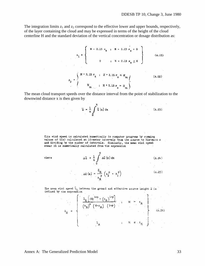
The integration limits z1 and z2 correspond to the effective lower and upper bounds, respectively,
of the layer containing the cloud and may be expressed in terms of the height of the cloud
centerline H and the standard deviation of the vertical concentration or dosage distribution as:
The mean cloud transport speeds over the distance interval from the point of stabilization to the
downwind distance x is then given by

DDESB TP 10, Change 3, June 1980
Annex A: The Generalized Prediction Model 34
A.2.4. Generalized Dosage Model
The generalized dosage mode for point and volume sources is given by the product of
four terms:
Dosage = {Peak Dosage Term} {Vertical Term}
(A.27)
{Lateral Term} {Depletion Term}
The Peak Dosage Term refers to the dosage on the downwind axis of the cloud (x, y=O,
z=H) and is defined by the expression
where
Q 2 = source strength
K = scaling coefficient used to convert input parameters into dimensionally consistent
Units
σy = standard deviation of the crosswind dosage distribution
σz = standard deviation of the vertical dosage distribution
A.3. APPLICATION OF THE GENERALIZED MODEL TO CONCENTRATIONS
PRODUCED BY QUASI-CONTINUOUS RELEASES
The concentrations produced by a quasi-continuous release in which the emission takes place
over a period of several minutes to several hours may be obtained by multiplying Equation
(A.27) by an Alongwind Term. For a release with a constant rate Q for a finite period r, the
Alongwind Term is given by
Note that the emission rate Q rather than the total source strength Q must be used in calculating
concentrations for this type of release.
In the case of an evaporative spill, the emission rate can be expected to decay exponentially
with time. For this type of release, the Alongwind Term is given by

DDESB TP 10, Change 3, June 1980
Annex A: The Generalized Prediction Model 35
where λ, is the evaporation coefficient, or the fraction of material evaporated per unit time. For
this type of release, the total source strength Q is entered in Equation (A.27). Additionally, the
initial alongwind dimension σxo is set equal to zero in the σx calculations.
A.4. APPLICATION OF THE GENERALIZED MODEL TO SURFACE DEPOSITIOH
BY GRAVITATIONAL SETTLING
Equation (A.27) may also be used to calculate the surface deposition due to gravitational
settling by replacing the Vertical Tern in Equation (A. 27) with the following expression:
A.5. ADJUSTMENTS OF THE GENERALIZED MODEL FOR CXANGES XN
METEOROLOGICAL STRUCTURE: THE STABILILTY-CHANGE MODEL
The generalized prediction model formulas, given above, assume steady-state conditions
throughout the reference air volume which may extend vertically for 3 kilometers and downwind
for 100 kilometers or more. In many instances, the steady-state assumption fails because of
changes in surface properties and atmospheric structure that occur along downwind cloud
trajectories. Techniques have been developed for adjusting the models to these changes which

DDESB TP 10, Change 3, June 1980
Annex A: The Generalized Prediction Model 36
treat the changes as step-changes in meteorological structure. At any specified travel time or
downwind-distance at which a step change in structure occurs, the transport and diffusion
processes are stopped; new sets of source and meteorological model inputs are calculated; and
the transport and diffusion process restarted with the new inputs. Thus, the procedures account
for the effects of step-changes in atmospheric stability on the concentration, dosage, and
deposition patterns in a gradual manner.
When the calculated generalized model distance exceeds the maximum downwind distance
(This maximum downwind distance is calculated by the product of the mean transport speed and
the maximum in-time duration for the stable regime.) that could exist in stable conditions, the
stability change-model is used. The maximum time duration of a stable nighttime regime is
generally 12 hours or less. Mean cloud transport speeds for stable regimes approximate 1 meter
per second (2.24 miles per hour) with a maxim distance of approximately 40 kilometers (25
miles). Whenever the calculated hazard distance exceeds the cloud-transport distance under
stable conditions, the stability-change model is used.
In the stability-change model, the mixing depth may be continuously varied by using the
following Vertical Term in the generalized models:
where
The only restriction to the use of the above Vertical Term is that the cloud must fill the mixing
layer and be completely mixed in the vertical (i.e., the concentration must be uniform with
height).

This page intentionally left blank

DDESB TP 10, Change 3, June 1980
Annex B: Toxicity for GB and VX as a Function of Exposure Time 37
ANNEX B
TOXICITY FOR GB AND VX AS A
FUNCTION OF EXPOSURE TIME

DDESB TP 10, Change 3, June 1980
Annex B: Toxicity for GB and VX as a Function of Exposure Time 38
CONTENTS
Page
B.l. GENERAL .............................................................................................................................40
B.2. THE BASIC MODEL ...........................................................................................................40
B.3. DOSAGE BUILDUP ............................................................................................................41

DDESB TP 10, Change 3, June 1980
Annex B: Toxicity for GB and VX as a Function of Exposure Time 39
LIST OF FIGURES
Page
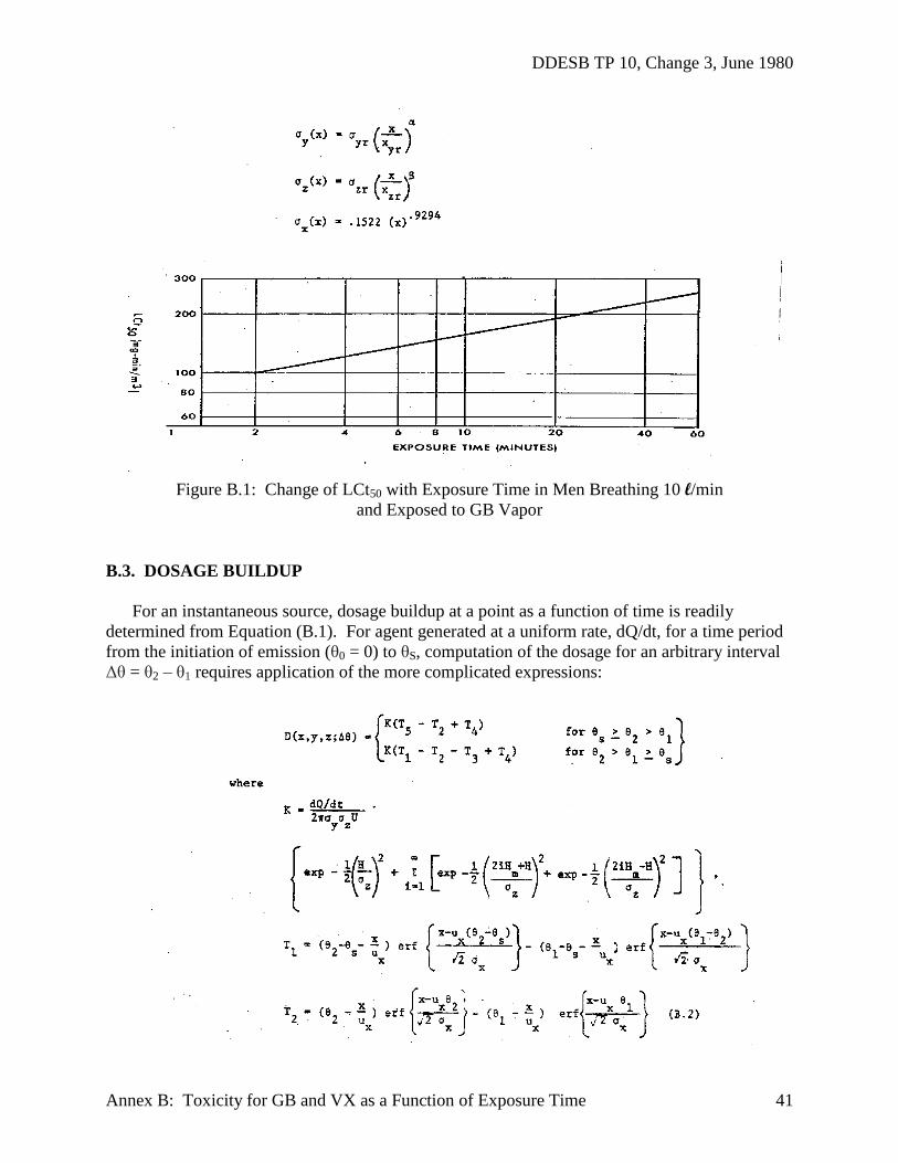
FIGURE B.l. Change of LCt50 with Exposure Time in Men Breathing 10 l/min and
Exposed to GB Vapor .............................................................................................41

DDESB TP 10, Change 3, June 1980
Annex B: Toxicity for GB and VX as a Function of Exposure Time 40
ANNEX B
TOXICITY FVR GB AND VX AS A
FUNCTION OF EXPOSURE TIME
B.1. GENERAL. This methodology is required to implement the changes in effective dosages
of GB and VX as a function of exposure time in agent clouds of nonuniform concentration.
Dosage, usually denoted D or Ct , is defined as the product of agent concentration at a point and
the time of exposure to those agent concentrations. Thus, exposure time for a given Ct is a factor
which influences the relationships between dosage and expected physiological response.
Increasing the exposure time to a given Ct results in a less severe toxic response. To produce the
same toxic response, higher Ct exposures are required for long exposure times than for short
ones. As an example, an estimated LCt50 value for a man breathing 10 l/min is 100 mg-min/m3
for a two minute exposure, while the LCt5O value is estimated as 210 mg-min/m3 f o r a 30-
minute exposure. The relationship between exposure time and LCt50 is shown in Figure B.1.1
Because the effective Ct exposure is dependent on the time, the degree of hazard will be reduced
in those accidents where the vapor is evolved slowly over a substantial time as compared with
nearly instantaneous releases such as would occur in detonation of a GB munition.
B.2. THE BASIC MODEL. The basic model for calculating peak dosage at ground level (y =
0, zero) as a function of distance and time may be expressed as
where
θ1, 2 = time subsequent to agent dissemination (θ2 > θ1)
Δθ = θ2 – θ1
________________________ 1Christensen, M. K., P. Cresthull, and F. W. Oberst. Chemical Warfare Laboratories Report No.
2266, ICt1-99 and LCt1-99 Estimates of GB Vapor for Man at Various Exposure Times, US Army
Chemical Warfare Laboratories, Army Chemical Center, MD. December 1958.
UNCLASSIFIED.
DDESB TP 10, Change 3, June 1980
Annex B: Toxicity for GB and VX as a Function of Exposure Time 41
Figure B.1: Change of LCt50 with Exposure Time in Men Breathing 10 l/min
and Exposed to GB Vapor
B.3. DOSAGE BUILDUP
For an instantaneous source, dosage buildup at a point as a function of time is readily
determined from Equation (B.1). For agent generated at a uniform rate, dQ/dt, for a time period
from the initiation of emission (θ0 = 0) to θS, computation of the dosage for an arbitrary interval
Δθ = θ2 – θ1 requires application of the more complicated expressions:

DDESB TP 10, Change 3, June 1980
Annex B: Toxicity for GB and VX as a Function of Exposure Time 42
A rationale was developed for the computation of the multiplier M by means of a numerical
procedure that allows for discrete changes in agent concentration as the cloud moves over a
ground location. In essence, a “pseudo” exposure time is determined through a sequence of
adjustments for successive time increments covering cloud passage. This “pseudo” exposure
time, which must be two minutes or greater for Equation (B.2) to be applicable, can be
considered essentially as an integrated average. The precise sequential mathematical procedure
is as follows:
Let ti = clock time in minutes
Ti = “pseudo” exposure time in minutes
ΔDi = dosage accumulation in interval i
Di = cumulative dosage to time ti
Doi = two-minute reference dosage
________________________
*In applying Equation (B.1) it should be noted that agent emission is defined in the expressions
as occurring from the origin (θ0=0) of the time scale to θs. For cases involving a series of
uniform generation rates, appropriate translations of the time scale (i,e., agent emission from θa
to θb) will be necessary.

DDESB TP 10, Change 3, June 1980
Annex B: Toxicity for GB and VX as a Function of Exposure Time 43
Subscript m denotes value computed from transport and diffusion model.
Subscript e denotes extrapolated value as indicated below.
a. Determine ΔD2m for interval t2-t1 from transport and diffusion model.
b. Compute (1) D2m = D1m + ΔD2m
(2) D2e = 0.827 D01 (T1 + t2 – t1)0.274
– (t1)0.274
c. Compare ΔD2m with ΔD2e
(1) If ΔD2m = ΔD2e, set T2 = T1 + t2 – t1
(2) If ΔD2m > ΔD2e, compute
a. Determine ΔDim for interval ti-ti-1 from transport and diffusion model.
b. Compute:
(1) Dim = D(i-l)m + ΔDim

DDESB TP 10, Change 3, June 1980
Annex B: Toxicity for GB and VX as a Function of Exposure Time 44
c. Compare ΔDim with ΔDie:
(1) If ΔDim = ΔDie, set Ti = Ti-1 + ti – ti-1
(2) If ΔDim > ΔDie, compute
For n increments, the reference two-minute dosage DOn is the value used in constructing the
generalized curves for GB and VX respiratory effects.
In using the above procedure, three precautions must be observed. Firstly, Ti cannot be
permitted to decrease below two minutes. Although such occurrence would generally be
unlikely, the possibility should be recognized in the computational procedure. Secondly, DOi
must be nondecreasing for successive increments. If DO(k+l) < DOk, as could occur through
consideration of very low dosages produced by the trailing edge of a cloud over an extended time
period, it is recommended that DO(k+l) be set equa1 to DOk before proceeding to the next interval.
Thirdly, since it is not apparent that the maximum value of DOi will always exceed the actua1
peak two-minute accumulation during cloud passage, a numerical comparison should be made,
with the larger value obviously accepted as the basis for hazard-distance estimation.

This page intentionally left blank
DDESB TP 10, Change 3, June 1980
Annex C: Method for Calculating Rates of Evaporation from Puddles of Liquid Toxic
Substances 45
ANNEX C
METHOD FOR CALCULATING RATES OF EVAPORATION
FROM PUDDLES OF LIQUID TOXIC SUBSTANCES

DDESB TP 10, Change 3, June 1980
Annex C: Method for Calculating Rates of Evaporation from Puddles of Liquid Toxic
Substances 46
CONTENTS
Page
C.l. GENERAL .............................................................................................................................48
C.2. THE REYNOLDS NUMBER ...............................................................................................48
C.3. THE MASS TRANSFER FACTOR .....................................................................................49
C.4. THE MASS TRANSFER COEFFICIENT ...........................................................................49
C.5. THE EVAPORATION RATE ..............................................................................................50
C.6. THE EVAPORATION RATE INTO STILL AIR ................................................................51

DDESB TP 10, Change 3, June 1980
Annex C: Method for Calculating Rates of Evaporation from Puddles of Liquid Toxic
Substances 47
LIST OF TABLES
Page
TABLE C.l. AGENT INPUT DATA ...........................................................................................51
TABLE C.2. AGENT PARAMETERS ........................................................................................52

DDESB TP 10, Change 3, June 1980
Annex C: Method for Calculating Rates of Evaporation from Puddles of Liquid Toxic
Substances 48
ANNEX C
METHOD FOR CALCULATING
RATES OF EVAPORATION
FROM PUDDLES OF LIQUID TOXIC SUBSTANCES
C.1. GENERAL
The general model for computing rates of evaporation from puddles of toxic substances is
presented in this Annex. Its principal value here is to enable analysts to calculate evaporation
rates for situations whose parameter values are out of the range of Figures 1, 2 and 3 in Section
3.4 of the Technical Paper. In particular, evaporation rates for toxic substances other than the
three chemical warfare agents, GB, VX, and HD, may be calculated by way of this model. For
completeness, input data used to compute evaporation rates for those three agents are also
provided in Table C.1.
The evaporation-rate model described herein was adapted from the Chemical Engineers
Handbook1, by Solomon2, for application to chemical hazard prediction problems. It is
reproduced here as it was originally resented in ORG 40, with the exception that all units of
measurement have been converted to the Metric system. The format is that of a “cookbook
recipe” for deriving evaporation rates.
C.2. THE REYNOLDS NUMBER
Determine the dimensionless Reynold's number, NRe, for the air flow from the equation
where
λ = downwind length of the puddle (m),
U = wind speed (m/sec),
ρ = density of the air (gm/cm3),
μ = viscosity of the air (poise (gm/cm . sec)).
________________________ 1Perry, M.H. (editor), Chemical Engineers’ Handbook, 3rd Edition, McGraw-Hill Book
Company, Inc., 1950.
2Solomon, I., et al, Methods of Estimating Hazard Distances for Accidents Involving Chemical
Agents (U), ORG Report No. 40, US Amy Munitions Command, Operations Research Group,
Edgewood Arsenal, MD, February 1970. CONFIDENTIAL.
DDESB TP 10, Change 3, June 1980
Annex C: Method for Calculating Rates of Evaporation from Puddles of Liquid Toxic
Substances 49
The density of air in gms/cm3 can be determined by
where
T = temperature (OK),
P = ambient pressure (atm).
The viscosity of air can be determined from
μ = e(4.36 + .002844T)
x 10-6
C.3. THE MASS TRANSFER FACTOR
From the Reynolds number, calculate the mass transfer factor, jm, as follows:
C.4. THE MASS TRANSFER COEFFICIENT
The mass transfer coefficient, Kg, is calculated by
where
Kg = mass transfer coefficient (gm-moles/sec . cm2),
Gm = molar mass velocity of air (gm-moles/sec . cm2),
(μ/ρd) = Schmidt number (dimensionless),
d = diffusivity (dimensionless).
The molar mass velocity of air can be determined by the formula
where MA = molecular weight of air 29 gms/gm mole
DDESB TP 10, Change 3, June 1980
Annex C: Method for Calculating Rates of Evaporation from Puddles of Liquid Toxic
Substances 50
The diffusivity of air, d, may be computed from
where
T = temperature (OK),
P = ambient pressure (atm),
VA = molecular volume of air at normal boiling point (cm3/gm mole),
VL = molecular volume of liquid at normal boiling point (cm3/mole),
ML = molecular weight of liquid (gm/gm mole),
MA = molecular weight of air, gms/gm mole.
The molecular volumes VA and VL can be determined from Table 10 in Section 8 of the cited
handbook. For the three chemical agents whose evaporation rates are presented in graphical
form, the necessary input data required for calculations is contained in Table C.1.
C.5. THE EVAPORATION RATE
The driving force for evaporation is the difference between the mole fractions of the agent at
the agent-air interface and in the main air stream. If the mole fraction in the air is assumed to be
negligible, the driving force can be approximated by the ratio of the vapor pressure of the agent
(at the prevailing temperature) to one atmosphere in equivalent units, as shown in the following
equation:
E = Kg . ML. PL / (760 . P) . 6.0 . 105
where
E = evaporation rate of liquid (gms/m2 min),
PL = vapor pressure of liquid at liquid air interface (mm Hg).

DDESB TP 10, Change 3, June 1980
Annex C: Method for Calculating Rates of Evaporation from Puddles of Liquid Toxic
Substances 51
TABLE C.1. AGENT INPUT DATA
AGENT
MOLECULAR WEIGHT
(gms/gm-mole)
MOLECULAR VOLUME
(cm3/gm mole)
VAPOR PRESSURE RELATIONSHIP
(mm Hg)
GB 140.1 148.5 log PL = 8.5916 – 2424.5/T
VX 267.4 342.5 log PL = 7.70897 – 3187.0/T HD 159.1 157.6 log PL = 38.525 – 4500.0T – 9.86 log T
C.6. THE EVAPORATION RATE INTO STILL AIR
This methodology is to be used when the incident occurs within a closed building or other
confined location that precludes the movement of air during the evaporation of the toxic liquid.
The evaporation rate into still air is calculated using the following semi-empirical equationl:
________________________ 1Rife, Richard. Calculation of Evaporation Rates for Chemical Agent Spills, Office of the
Project Manager for Chemical Demilitarization and Installation Restoration, Aberdeen Proving
Ground, MD. (Equation 17). October 1978

DDESB TP 10, Change 3, June 1980
Annex C: Method for Calculating Rates of Evaporation from Puddles of Liquid Toxic
Substances 52
In calculating the Reynold's number, the effect of the agent vapors or the air viscosity and
density will be ignored.
The following agent parameters apply:
TABLE C.2. AGENT PARAMETERS
ML σ Ɛ/k (Ok)
air 29.0 3.711 78.6
GB 140.1 6.25 521
VX 267.42 8.26 691
HD 159.1 6.37 593
The remaining intermediate variables use the same auxiliary relationships as for moving air
conditions.

This page intentionally left blank

DDESB TP 10, Change 3, June 1980
Annex D: Methods for Calculating Hazards for Explosive Dissemination of VX and HD 53
ANNEX D
METHODS FOR CALCULATING HAZARDS FOR
EXPLOSIVE DISSEMINATION OF VX AND HD
DDESB TP 10, Change 3, June 1980
Annex D: Methods for Calculating Hazards for Explosive Dissemination of VX and HD 54
CONTENTS
Page
D.l. GENERAL .............................................................................................................................56
D.2. THE METHOD FOR VX .....................................................................................................56
D.3. THE METHOD FOR HD .....................................................................................................58

DDESB TP 10, Change 3, June 1980
Annex D: Methods for Calculating Hazards for Explosive Dissemination of VX and HD 55
LIST OF FIGURES
Page
Figure D.l. Hazard Distances for Explosively Disseminated Agent VX ......................................57
Figure D.2. Nomograph for the Determination of the Final Reference Value for Agent HD ......59
LIST OF TABLES
Table D.1. Hazard Distances for Explosively Disseminated Agent HD ......................................60

DDESB TP 10, Change 3, June 1980
Annex D: Methods for Calculating Hazards for Explosive Dissemination of VX and HD 56
ANNEX D
METHODS FOR CALCULATING HAZARDS FOR
EXPLOSIVE DISSEMINATION OF VX AND HD
D.1. GENERAL
This annex presents an interim method for computing the hazard distances associated with
explosive dissemination of agents VX and HD.
Explosive dissemination of these persistent agents yields source clouds characterized by
vapors as well as liquid droplets whose diameters span a considerable size range (i.e., from
molecular diameters to thousands of microns). Thus, there are two types of threats from
explosives involving those agents: (1) the percutaneous, or skin-absorption, threat due to the
impaction of droplets on personnel, and (2) the respiratory threat due to inhalation of either the
vapor or the aerosol.
Given that data existed to describe the particle size distribution in the aerosol, the settling
velocities of droplet sizes in the atmosphere, and the efficiency of droplet impaction on
personnel, the Generalized Prediction Model described in Annex A would be applied,
incrementally, to the vapor and to each of several droplet size ranges in the aerosol. The results
of those calculations would be summed at each point in the challenged area. The hazard distance
associated with the combined vapor/aerosol threat would be specified as the required hazard
distance. However, adequate data simply do not exist. Therefore, empirical methods were
derived from analyses of test data. Those methods, originally described in ORG 4013
, have been
simplified and adapted for use here. A complete description of the data base, and an explanation
of this specialized methodology are presented on pages 140 thru 160 of ORG 40.
D.2. METHOD FOR VX
Figure D.1. shows the “1% lethality” hazard. distance, in feet, associated with the release of
VX vapor and aerosol thru explosive dissemination. Each line shown on that figure represents a
Pasquill stability category. Lines A and B represent lapse conditions, in which cases the
predominant hazard arises from the percutaneous challenge. Hazards under conditions of neutral
stability (i.e., C and D) and weak inversions (i.e., E) are also dominated by percutaneous effects.
Maximum hazards under strong inversions (i.e., F) arise solely from the long-distance travel of
the vapor under the inversion cap.

DDESB TP 10, Change 3, June 1980
Annex D: Methods for Calculating Hazards for Explosive Dissemination of VX and HD 57
Figure D.1: Hazard Distance for Explosively Disseminated VX

DDESB TP 10, Change 3, June 1980
Annex D: Methods for Calculating Hazards for Explosive Dissemination of VX and HD 58
Application of Figure D.1. to problems involving accidental explosive releases of agent VX
is as follows:
(1) Determine the number and type of munitions involved in the explosive releases.
(2) Compute the total amount of agent released.
(3) Enter that quantity of agent (in pounds) into the ordinate scale in Figure D.1.
(4) Proceed across Figure D.1. to the appropriate meteorological stability category of
interest. [The stability category can be determined from Table 1, 16.]
(5) Read the maximum credible hazard distance, for 1% lethalities, on the abscissa scale.
D.3. THE METHOD FOR HD
Figure D.2. and Table 9.1. must both be used to determine hazard distances associated with
accidental explosive releases of agent XD. The method is as follows:
(1) The micrometeorologica1 conditions of interest (i.e., windspeed, temperature, and
stability category) must be determined. Temperature may be estimated from historical data.
Stability category and windspeed may be estimated from Table 1, page 16.
(2) Determine the fraction of agent airborne as vapors and droplets from Figure D.2. as
follows:
(a) Enter ordinate M on Figure D.2. at the appropriate windspeed value.
(b) Construct a straight line from the windspeed on ordinate M, thru the correct
temperature on diagonal N, to a point on ordinate P.
(c) From that point on ordinate P construct a straight line, thru the stability category
on diagonal Q, to a point on ordinate R.
(d) From that point on ordinate R construct a straight line, thru the 4.2" Mortar mark
on the diagonal, to a point on the ordinate S.
(3) Using the value of S determined in the previous step, compute the Final Reference
Value from the following equation:
DDESB TP 10, Change 3, June 1980
Annex D: Methods for Calculating Hazards for Explosive Dissemination of VX and HD 59
Figure D.2: Nomograph for Determination of the Final Reference Value for Agent HD
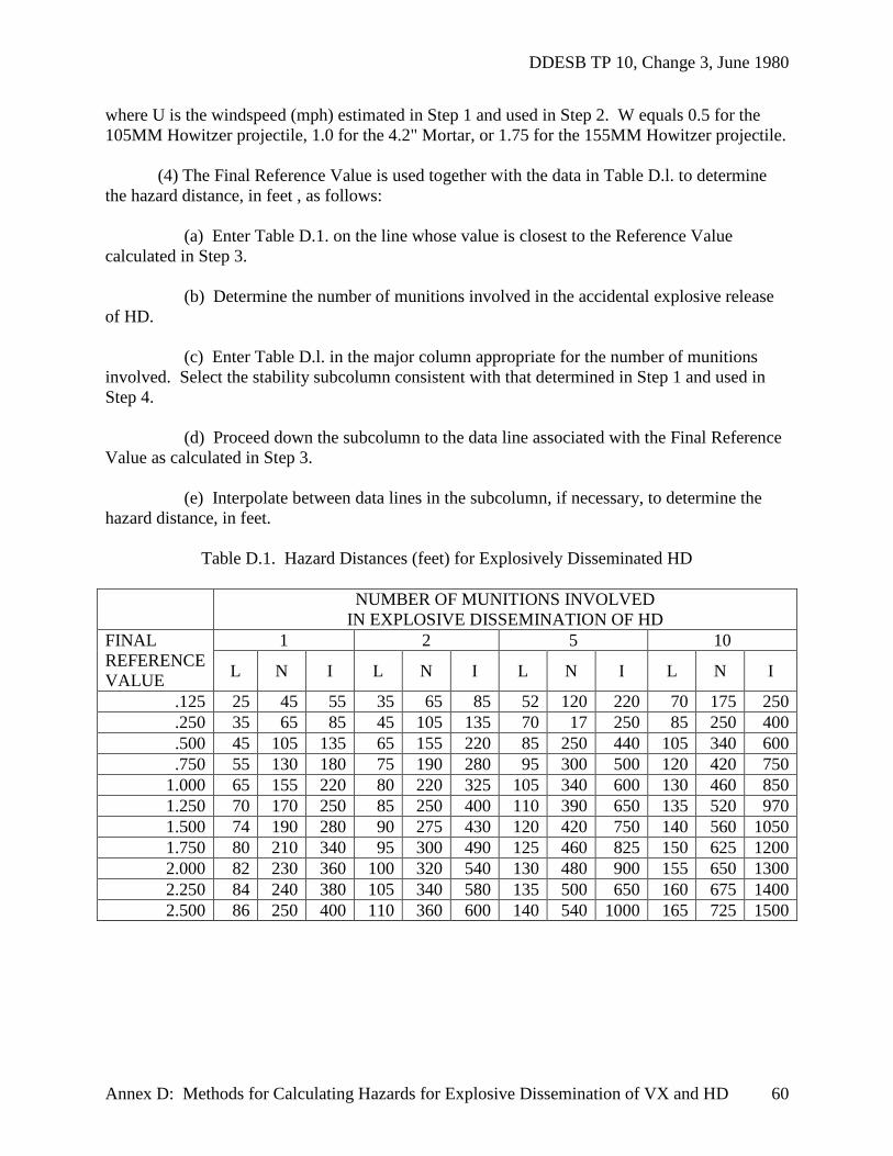
DDESB TP 10, Change 3, June 1980
Annex D: Methods for Calculating Hazards for Explosive Dissemination of VX and HD 60
where U is the windspeed (mph) estimated in Step 1 and used in Step 2. W equals 0.5 for the
105MM Howitzer projectile, 1.0 for the 4.2" Mortar, or 1.75 for the 155MM Howitzer projectile.
(4) The Final Reference Value is used together with the data in Table D.l. to determine
the hazard distance, in feet , as follows:
(a) Enter Table D.1. on the line whose value is closest to the Reference Value
calculated in Step 3.
(b) Determine the number of munitions involved in the accidental explosive release
of HD.
(c) Enter Table D.l. in the major column appropriate for the number of munitions
involved. Select the stability subcolumn consistent with that determined in Step 1 and used in
Step 4.
(d) Proceed down the subcolumn to the data line associated with the Final Reference
Value as calculated in Step 3.
(e) Interpolate between data lines in the subcolumn, if necessary, to determine the
hazard distance, in feet.
Table D.1. Hazard Distances (feet) for Explosively Disseminated HD
NUMBER OF MUNITIONS INVOLVED
IN EXPLOSIVE DISSEMINATION OF HD
FINAL
REFERENCE
VALUE
1 2 5 10
L N I L N I L N I L N I
.125 25 45 55 35 65 85 52 120 220 70 175 250
.250 35 65 85 45 105 135 70 17 250 85 250 400
.500 45 105 135 65 155 220 85 250 440 105 340 600
.750 55 130 180 75 190 280 95 300 500 120 420 750
1.000 65 155 220 80 220 325 105 340 600 130 460 850
1.250 70 170 250 85 250 400 110 390 650 135 520 970
1.500 74 190 280 90 275 430 120 420 750 140 560 1050
1.750 80 210 340 95 300 490 125 460 825 150 625 1200
2.000 82 230 360 100 320 540 130 480 900 155 650 1300
2.250 84 240 380 105 340 580 135 500 650 160 675 1400
2.500 86 250 400 110 360 600 140 540 1000 165 725 1500

DDESB TP 10, Change 3, June 1980
DD Form 1473 61
This page intentionally left blank

DDESB TP 10, Change 3, June 1980
Distribution List 62
DISTRIBUTION LIST
No. of Copies
Chairman 25
Department of Defense Explosives Safety Board
2461 Eisenhower Avenue
Alexandria, VA 22331
Office of Secretary of Defense (MRA&L) 1
ATTN: Mr. H. Metcalf
Washington, DC 20301
Director of Defense Research & Engineering 1
Department of Defense
Washington, DC 20301
Defense Technical Information Center 12
ATTN: DDC-TC
Cameron Station
Alexandria, VA 22314
Commander in Chief 5
US Army Europe & Seventh Army
ATTN: AEAGA-BE
APO New York 09403
Commander
US Army Materiel Development & Readiness Command
ATTN: DRCMM-ST 2
DRCSA-CS 2
DRCSA-NS 2
DRCSF 2
DRCSG 2
DRCSS 2
5001 Eisenhower Avenue
Alexandria, VA 22333
Commander 1
US Army Armament Research & Development Command
ATTN: DRDAR-SF
Dover, N. J. 07801
DDESB TP 10, Change 3, June 1980
Distribution List 63
DISTRIBUTION LIST, CONTINUE
No. of Copies
Commander
US Army Armament Materiel Readiness Command
ATTN: DRSAR-LE 1
DRSAR-PEL 1
DRSAR-SF 1
DRSAR-SS 1
DRSAR-MA 1
DRSAR-LEC 1
Rock Island, IL 61201
Chief of Engineers 2
Department of the Army
ATTN: DAEN-MCE-D
Washington, DC 20314
Commander 2
US Army Test & Evaluation Command
ATTN: DRSTE-ST
Aberdeen Proving Ground, MD 21005
Commander 1
MERADCOM
ATTN: DRDME-BR (Mr. McMillan)
Ft. Belvoir, VA 22060
Commander 2
US Army Missile Command
ATTN: DRSMI-0
Redstone Arsenal, AL 35809
Mr. Billy K. W. Fu, SDSSI-S 1
Safety Engineer
Sierra Army Depot
Herlong, CA 96113
Project Manager, Chemical Demilitarization and 2
Installation Restoration
ATTN: DRC'PM-DR-T
Aberdeen Proving Ground, MD 21010

DDESB TP 10, Change 3, June 1980
Distribution List 64
DISTRIBUTION LIST, CONTINUED
No. of Copies
Commander
Anniston Army Depot
ATTN: SDSAN-SF 1
SDSAN-CS 1
Anniston, AL 36201
Commander 3
Dugway Proving Ground
ATTN: STEDP-SA, Paul Carlson, Meteorology
Dugway, Utah 84022
Commander 2
84th Ordnance Battalion
APO New York 09189
Mr. Jerry Litwok 1
ATTN: SDSSE-PS
Senaca Army Depot
Romulus, X.Y. 14541
Commander
Chemical Systems Laboratory
US Army Armament Research & Development Command
ATTN: DRDAR-CLE 2
DRDAR-CLF 2
DRDAR-CLR 2
DRDAR-CLS 2
DRDAR-CLT 2
DRDAR-CLY 2
DRSTE-ST 2
Aberdeen Proving Ground, MD 21010
Commander 2
267th Chemical Company
APO San Francisco 96305
Mr. Pete Rutledge 2
US Army Materiel Development & Readiness Command
ATTN: DRCSF-S
5001 Eisenhower Avenue
Alexandria, VA 22333

DDESB TP 10, Change 3, June 1980
Distribution List 65
DISTRIBUTION LIST, CONTINUED
No. of Copies
Office of Assistant Secretary of the Army 1
ATTN: OASA(IL&FM)
Washington, DC 20310
Chief of Research, Development & Acquisition 1
Department of the Army
Washington, DC 20310
HQDA (DAPE-HRS) 2
(DALO)-SMD) 2
(DAMO-SSC) 2
Washington, DC 20310
HQDA (DAMO-SSN) 1
Washington, DC 20310
US Army Nuclear and Chemical Surety Group 5
ATTN: MONA-SU-MOSG
Bldg 2073, North Area
Ft. Belvoir, VA 22060
Commander 1
US Army Forces Command
ATTN: AFPR-PSS
Ft. McPherson, GA 30330
Commander
US Army Training & Doctrine Command 1
ATTN: ATRP-PD-S
Ft. Monroe, VA 23651
Commander
Lexington-Blue Grass Army Depot
ATTN: SDSRR-LX-AS 1
SDSRR-LX-QA
Lexington, KY 40507

DDESB TP 10, Change 3, June 1980
Distribution List 66
DISTRIBUTION LIST, CONTINUED
No. of Copies
Commander 3
Newport Army Ammunition Plant
P.O. Box 121
ATTN: SARNE-S/SARNE-SE
Newport, IN 47996
Commander 3
Pine Bluff Arsenal
ATTN: SARPB-SA/SARPB&P
Pine Bluff, AR 71601
Commander 4
Pueblo Army Depot
ATTN: SDSTE-PU-ME/SDSTE-PU-A
Pueblo, CO 81001
Redstone Arsenal Chemical School 2
US Army Missile & Munitions Center & School
Redstone Arsenal, AL 35809
Commander 3
Rocky Mountain Arsenal
ATTN: SARRM-SAF
Commerce City
Colorado 80022
Commander 6
Tooele Army Depot
ATTN: SDSTE-ADS
Tooele, UT 84074
Comnander 2
60th Ordnance Group
APO New York 09052
National Transportation Safety Board 1
ATTN: TE-40, Ms. Becky Rote
800 Independence Ave., S.W.
Washington, DC 20594

DDESB TP 10, Change 3, June 1980
Distribution List 67
DISTRIBUTION LIST, CONTINUED
No. of Copies
Commander 3
Umatilla Army Depot
ATTN: SDSTE-UM/SDSTE-UAS
Hermiston, OR 97838
Director 4
DARCOM Field Safety Activity
ATTN: DRXOS-C
Charlestown, IN 47111
Commander 4
US Army Materiel Development & Readiness Command
Surety Field Office, ATTN: DRCSA-NF
Dover, N.J. 07801
Director 3
DARCOM Ammunition Center
Savanna Army Depot
ATTN: SARAC-AS/SARAC-DEO
Savanna, IL 61074
Commander 3
US Army Ordnance and Chemical Center & School
ATTN: ATSL-CD-MS
Aberdeen Proving Ground, MD 21005
Commander 2
US Army Environmental Hygiene Agency
ATTN: HSE-EA-A
Aberdeen Proving Ground, MD 21010
Commandant 5
USAMMCS
ATTN: ATSK-DT-MU-EOD
Redstone Arsenal, AL 35809
Chief of Naval Materiel 1
ATTN: MAT034B
Washington, DC 20360

DDESB TP 10, Change 3, June 1980
Distribution List 68
DISTRIBUTION LIST, CONTINUED
No. of Copies
Chief of Naval Operations 1
ATTN: OP-411
Washington, DC 20350
Mr. Stanley S. Grossel 1
Engineering Fellow
Process Design Section
Hoffmann-La Roche Inc.
Nutley, N.J. 07110
Capt Fredric Jonasz, USN 1
OPNAV (OP-411)
Rm 4B524, Pentagon
Washington, DC 20350
Commander 1
Naval Sea Systems Command
ATTN: SEA-09B4
Washington, DC 20360
Commander 2
Naval Surface Weapons Center
White Oak Laboratory
ATTN: CR-10
Silver Spring, MD 20910
Commanding Officer 1
Naval Ammunition Depot
ATTN: NAPEC
Crane, IN 27522
Commander
Naval Surface Weapons Center
ATTN: Code CG302 1
Code CG-32 1
Dahlgren, Virginia 22448

DDESB TP 10, Change 3, June 1980
Distribution List 69
DISTRIBUTION LIST, CONTINUED
No. of Copies
Commander 1
Naval Surface Weapons Center
White Oak Laboratory
ATTN: Code CA-13 (Lewis C. Dixon)
Silver Spring, MD 20910
Commander 2
Naval EOD Facility
ATTN: Army Chemical Office
Indian Head, MD 20640
Air Force Systems Command 1
ATTN: IGFG (Mr. Ken Nogle)
Andrews Air Force Base
Washington, DC 20334
Defense Nuclear Agency 1
Kirtland Air Force Base
Albuquerque, N.M. 87417
Director of Aerospace Safety 3
HQ USAF
ATTN: AFISC/SEW
Norton AFB, CA 92409
LtCol Paul Fallon 1
HQ AMD/RDU
Brooks AFB, TX 78235
Commander 2
Air Weather Service
ATTN: DNPA
Scott AFB, IL 62225
UQ USAF 1
USAF Scientific Advisory Board
Ad Hoc Committee on Defense Chemical Systems
ATTN: LTC John M. Howell, Jr., AF/NB
Room 5D982, Pentagon
Washington, DC

DDESB TP 10, Change 3, June 1980
Distribution List 70
DISTRIBUTION LIST, CONTINUED
No. of Copies
Dr. B. John Garrick 1
400 Orangethrope Ave.
Anaheim, CA 92802
Dr. H. E. Cramer 1
H. E. Cramer Co., Inc.
P.O. Box 9299
Salt Lake City, UT 84109
Dr. George Miley 1
Geomet, Inc.
15 Firstfield Road
Gaithersburg, MD 20760
Mr. Ed Haggerty 1
Tracor Jitco
1776 E. Jefferson Street
Rockville, MD 20852