Embed Size (px)
Citation preview
TD 310 DCPS Primer April 2019
DCPS Theoretical Primer Current and Wave

Page 2 April 2019 - TD 310 DCPS Theoretical Primer
Preliminary Edition 16th December 2015
1st revision 13th May 2016
2nd revision 9th April 2019 Added Acoustic Wave
© Copyright: Aanderaa Data Instruments AS

April 2019 - TD 310 DCPS Theoretical Primer Page 3
Contact information:
Aanderaa Data Instrument AS
PO BOX 103, Midttun
5843 Bergen, NORWAY
Visiting address:
Sandalsringen 5b
5843 Bergen, Norway
TEL: +47 55 604800
FAX: +47 55 604801
EMAIL: [email protected]
WEB: http://www.aanderaa.com

Page 4 April 2019 - TD 310 DCPS Theoretical Primer
Table of Contents
Introduction ................................................................................................................... 6
Purpose and scope .............................................................................................................. 6
CHAPTER 1 The Doppler principle .............................................................................. 7
1.1 The Doppler Effect ......................................................................................................... 7 1.2 Doppler shifts using acoustic scatterers ......................................................................... 8 1.3 Decomposition of Doppler shift / radial motion ............................................................... 8
CHAPTER 2 Narrowband / Broadband – principles of operation................................ 10
2.1 Geometry and features of the Aanderaa DCPS ........................................................... 10 2.2 Narrowband Doppler Processing ................................................................................. 11 2.3 Broadband Doppler Processing ................................................................................... 11
2.3.1 Correlation factor ................................................................................................... 14 2.3.2 Ambiguity ............................................................................................................... 15 2.3.3 Limitation in the automatic ambiguity solution ........................................................ 17 2.3.4 From signal transmission to reception ................................................................... 17 2.3.5 Cell Spacing function ............................................................................................. 18 2.3.6 Multiple columns - surface or instrument reference functions................................. 19
CHAPTER 3 Calculation of vertical and horizontal currents ....................................... 20
3.1 Obtaining currents from multiple levels above/below the sensor .................................. 20 3.1.1 Relationship between current measured at beams and earth referenced current. .. 21 3.1.2 Transformation from the instrument reference system to the earth reference system ...................................................................................................................................... 22
3.2 Compensation for tilt and rotation in each measurement (ping) ................................... 24 3.3 Surface current measurements .................................................................................... 25
CHAPTER 4 The DCPS produces high quality data ................................................... 26
4.1 Innovative three beam solution .................................................................................... 26 4.2 Calculating the noise levels/standard deviation ............................................................ 27 4.3 DCPS Narrowband internal processing –ARMA model .......................................... 27
CHAPTER 5 Limitations of Doppler Current Profilers ................................................. 28
5.1 Influence of acoustic side lobes and the contaminated zone close to surface/bottom .. 28 5.2 Total measurement range ............................................................................................ 30 5.3 Blanking distance closest to the instrument ................................................................. 30 5.4 Random and systematic errors .................................................................................... 31
5.4.1 Beam separation ................................................................................................... 31 5.4.2 Echo intensity and backscatters ............................................................................ 31
CHAPTER 6 Acoustic Waves ..................................................................................... 33
6.1 Waves explained ......................................................................................................... 33 6.1.1 Deep water waves: ................................................................................................ 35 6.1.2 Shallow water waves: ............................................................................................ 35
CHAPTER 7 Measuring waves with an Acoustic Doppler Profiler .............................. 37

April 2019 - TD 310 DCPS Theoretical Primer Page 5
CHAPTER 8 Adaptive transmission pulse to optimize the wave measurement accuracy ..................................................................................................................... 42
8.1 Sensor self-noise ......................................................................................................... 42 8.2 Resolving ambiguities .................................................................................................. 43 8.3 Adaptive transmission pulse ........................................................................................ 46
CHAPTER 9 Wave frequency bandwidth limitations and cut-off period ...................... 49
CHAPTER 10 Wave direction ..................................................................................... 52
CHAPTER 11 Automatic cell location ......................................................................... 57
CHAPTER 12 Quality parameters .............................................................................. 58
CHAPTER 13 Parameters calculation - mathematical formulas ................................. 59
CHAPTER 14 References .......................................................................................... 63

Page 6 April 2019 - TD 310 DCPS Theoretical Primer
Introduction
Purpose and scope
This manual gives a basic and simplified theoretical background to the measurement principles of Acoustic Doppler Current Profilers with focus on the Aanderaa Doppler Current Profiling Sensor (DCPS 5400/5402/5403). This manual gives a basic and simplified theoretical background to the measurement of waves using a SeaGuardII DCP Wave.
April 2019 - TD 310 DCPS Theoretical Primer Page 7
CHAPTER 1 The Doppler principle
This chapter gives a basic description of the Doppler principle and how it could be used to measure relative radial velocity between different objects.
1.1 The Doppler Effect
Acoustic Doppler Current Profilers measure water velocity using a principle of physics discovered by Christian Johann Doppler (1842). The Doppler effect relates to the change in frequency for an observer moving relative to a source of sound or light. Doppler first stated his principle in the article, ‘Concerning the colored light of double stars and some other constellations in the heavens’.
In daily life a common example of the Acoustic Doppler effect or Doppler shift is the siren of an ambulance as it approaches, passes and recedes from an observer. Compared to the emitted frequency, the received frequency is higher during the approach, identical at the instant of passing by, and lower during recession. When the source of the waves is moving towards the observer, each successive wave crest is emitted from a position closer to the observer than the previous wave. Therefore, each wave takes slightly less time to reach the observer than the previous wave. Hence, the time between the arrivals of successive wave crests at the observer is reduced, causing an increase in the frequency (compressed sound waves). Conversely, if the source of waves is moving away from the observer, each wave is emitted from a position farther from the observer than the previous wave, so the arrival time between successive waves is increased, reducing the frequency. The distance between successive wave fronts is then increased (stretched out sound waves). The total Doppler effect result therefore from motion of the source and motion of the observer.
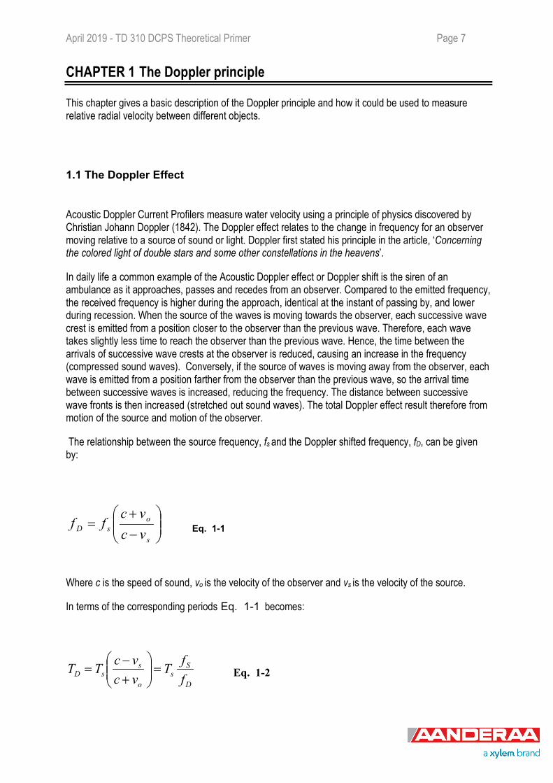
The relationship between the source frequency, fs and the Doppler shifted frequency, fD, can be given by:
−+
=s
osD vc
vcff Eq. 1-1
Where c is the speed of sound, vo is the velocity of the observer and vs is the velocity of the source.
In terms of the corresponding periods Eq. 1-1 becomes:
D
Ss
o
ssD f
fTvcvcTT =
+−
= Eq. 1-2
Page 8 April 2019 - TD 310 DCPS Theoretical Primer
1.2 Doppler shifts using acoustic scatterers
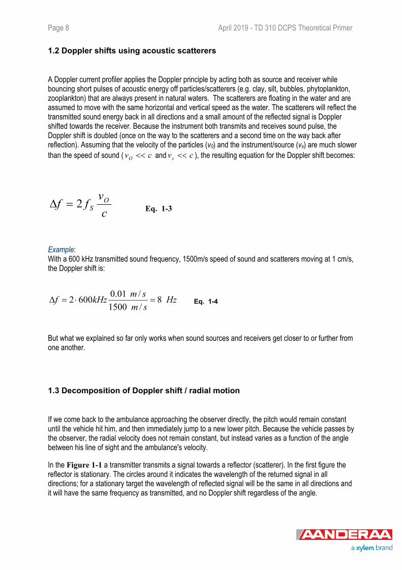
A Doppler current profiler applies the Doppler principle by acting both as source and receiver while bouncing short pulses of acoustic energy off particles/scatterers (e.g. clay, silt, bubbles, phytoplankton, zooplankton) that are always present in natural waters. The scatterers are floating in the water and are assumed to move with the same horizontal and vertical speed as the water. The scatterers will reflect the transmitted sound energy back in all directions and a small amount of the reflected signal is Doppler shifted towards the receiver. Because the instrument both transmits and receives sound pulse, the Doppler shift is doubled (once on the way to the scatterers and a second time on the way back after reflection). Assuming that the velocity of the particles (v0) and the instrument/source (vs) are much slower than the speed of sound ( cvO << and cvs << ), the resulting equation for the Doppler shift becomes:
cv
ff OS2=∆ Eq. 1-3
Example: With a 600 kHz transmitted sound frequency, 1500m/s speed of sound and scatterers moving at 1 cm/s, the Doppler shift is:
HzsmsmkHzf 8
/1500/01.06002 =⋅=∆ Eq. 1-4
But what we explained so far only works when sound sources and receivers get closer to or further from one another.
1.3 Decomposition of Doppler shift / radial motion
If we come back to the ambulance approaching the observer directly, the pitch would remain constant until the vehicle hit him, and then immediately jump to a new lower pitch. Because the vehicle passes by the observer, the radial velocity does not remain constant, but instead varies as a function of the angle between his line of sight and the ambulance's velocity.
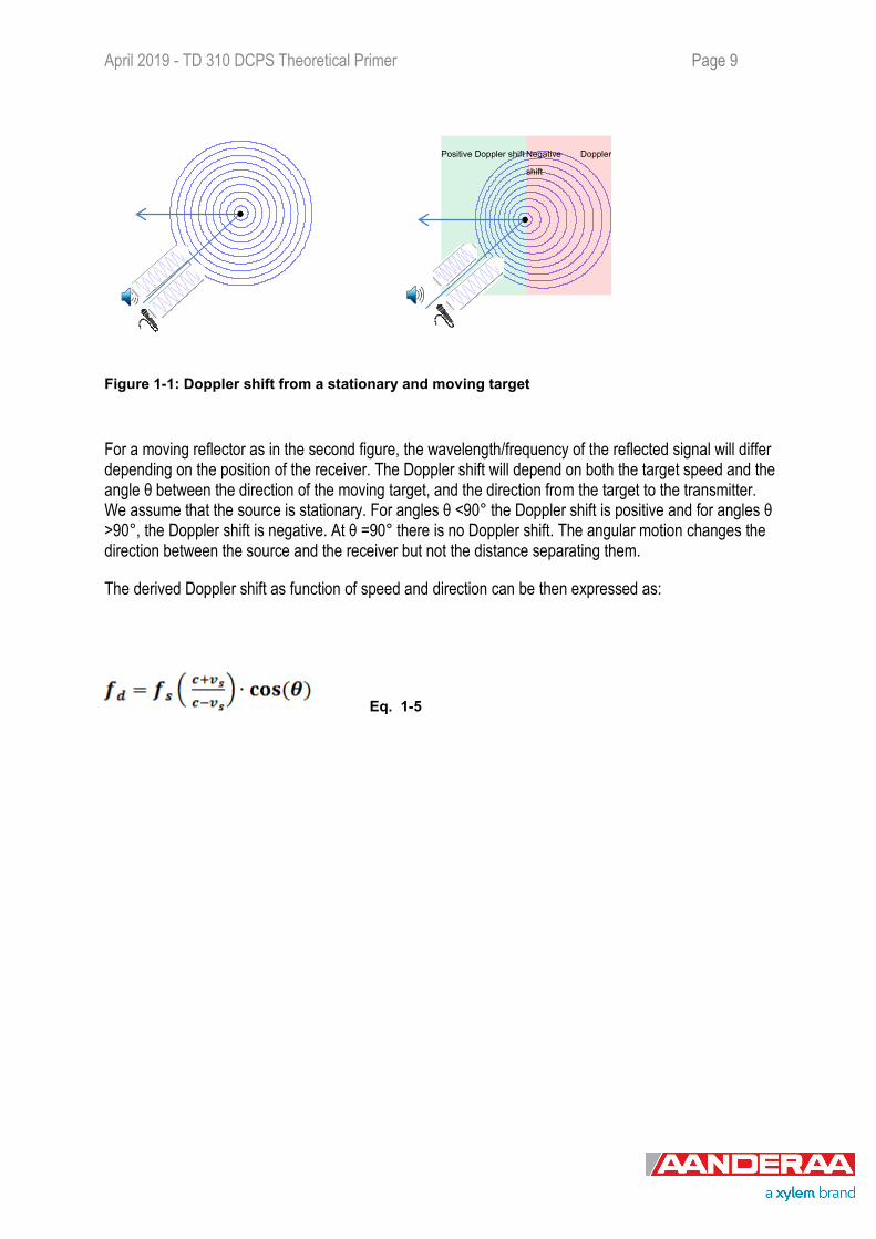
In the Figure 1-1 a transmitter transmits a signal towards a reflector (scatterer). In the first figure the reflector is stationary. The circles around it indicates the wavelength of the returned signal in all directions; for a stationary target the wavelength of reflected signal will be the same in all directions and it will have the same frequency as transmitted, and no Doppler shift regardless of the angle.
April 2019 - TD 310 DCPS Theoretical Primer Page 9
Figure 1-1: Doppler shift from a stationary and moving target
For a moving reflector as in the second figure, the wavelength/frequency of the reflected signal will differ depending on the position of the receiver. The Doppler shift will depend on both the target speed and the angle θ between the direction of the moving target, and the direction from the target to the transmitter. We assume that the source is stationary. For angles θ <90° the Doppler shift is positive and for angles θ >90°, the Doppler shift is negative. At θ =90° there is no Doppler shift. The angular motion changes the direction between the source and the receiver but not the distance separating them.
The derived Doppler shift as function of speed and direction can be then expressed as:
Eq. 1-5
0
200
400
600
800
1000
60.4-0
.200
.2
4
0
200
400
600
800
1000
60.4-0
.200
.2.4
6
Negative Doppler
shift
Positive Doppler shift
0
200
400
600
800
1000
60.4-0
.200
.2
4
0
200
400
600
800
1000
0.6-0
.4-0.2
00.2
0.4
.6
Page 10 April 2019 - TD 310 DCPS Theoretical Primer
CHAPTER 2 Narrowband / Broadband – principles of operation
2.1 Geometry and features of the Aanderaa DCPS
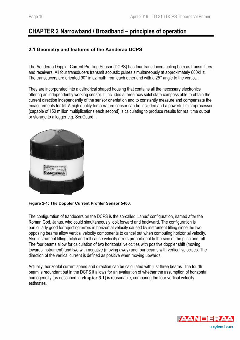
The Aanderaa Doppler Current Profiling Sensor (DCPS) has four transducers acting both as transmitters and receivers. All four transducers transmit acoustic pulses simultaneously at approximately 600kHz. The transducers are oriented 90° in azimuth from each other and with a 25° angle to the vertical. They are incorporated into a cylindrical shaped housing that contains all the necessary electronics offering an independently working sensor. It includes a three axis solid state compass able to obtain the current direction independently of the sensor orientation and to constantly measure and compensate the measurements for tilt. A high quality temperature sensor can be included and a powerfull microprocessor (capable of 150 million multiplications each second) is calculating to produce results for real time output or storage to a logger e.g. SeaGuardII.
Figure 2-1: The Doppler Current Profiler Sensor 5400.
The configuration of tranducers on the DCPS is the so-called ‘Janus’ configuration, named after the Roman God, Janus, who could simultaneously look forward and backward. The configuration is particularly good for rejecting errors in horizontal velocity caused by instrument tilting since the two opposing beams allow vertical velocity components to cancel out when computing horizontal velocity. Also instrument tilting, pitch and roll cause velocity errors proportional to the sine of the pitch and roll. The four beams allow for calculation of two horizontal velocities with positive doppler shift (moving towards instrument) and two with negative (moving away) and four beams with vertical velocities. The direction of the vertical current is defined as positive when moving upwards. Actually, horizontal current speed and direction can be calculated with just three beams. The fourth beam is redundant but in the DCPS it allows for an evaluation of whether the assumption of horizontal homogeneity (as described in chapter 3.1) is reasonable, comparing the four vertical velocity estimates.
April 2019 - TD 310 DCPS Theoretical Primer Page 11
Utilizing four beams also makes it possible to calculate four different three-beam solutions by omitting one of the transducers. This can be useful in the case when for example one of the beams are receiving erroneous data caused by objects like mooring lines and floats that are not moving with the water flow. The DCPS has this ability built in (refer chapter 4.1). It gives enhanced possibilities to understand the prevailing conditions and obtain high quality data.
The DCPS has two user selectable modes to measure currents; narrowband or broadband.
2.2 Narrowband Doppler Processing
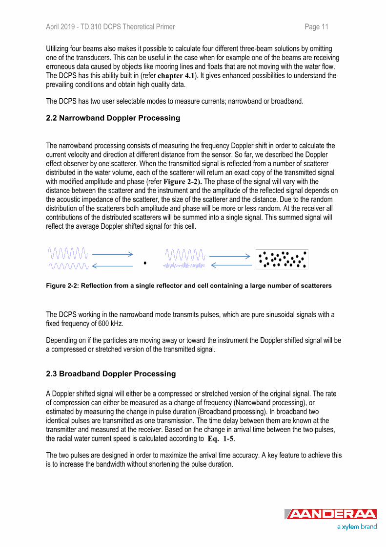
The narrowband processing consists of measuring the frequency Doppler shift in order to calculate the current velocity and direction at different distance from the sensor. So far, we described the Doppler effect observer by one scatterer. When the transmitted signal is reflected from a number of scatterer distributed in the water volume, each of the scatterer will return an exact copy of the transmitted signal with modified amplitude and phase (refer Figure 2-2). The phase of the signal will vary with the distance between the scatterer and the instrument and the amplitude of the reflected signal depends on the acoustic impedance of the scatterer, the size of the scatterer and the distance. Due to the random distribution of the scatterers both amplitude and phase will be more or less random. At the receiver all contributions of the distributed scatterers will be summed into a single signal. This summed signal will reflect the average Doppler shifted signal for this cell.
Figure 2-2: Reflection from a single reflector and cell containing a large number of scatterers
The DCPS working in the narrowband mode transmits pulses, which are pure sinusoidal signals with a fixed frequency of 600 kHz.
Depending on if the particles are moving away or toward the instrument the Doppler shifted signal will be a compressed or stretched version of the transmitted signal.
2.3 Broadband Doppler Processing A Doppler shifted signal will either be a compressed or stretched version of the original signal. The rate of compression can either be measured as a change of frequency (Narrowband processing), or estimated by measuring the change in pulse duration (Broadband processing). In broadband two identical pulses are transmitted as one transmission. The time delay between them are known at the transmitter and measured at the receiver. Based on the change in arrival time between the two pulses, the radial water current speed is calculated according to Eq. 1-5.
The two pulses are designed in order to maximize the arrival time accuracy. A key feature to achieve this is to increase the bandwidth without shortening the pulse duration.
Page 12 April 2019 - TD 310 DCPS Theoretical Primer
The accuracy of the time measurement for a given pulse is dependent on the bandwidth;
Eq. 2-1
By increasing the bandwidth, the uncertainty related to the time estimate will be reduced proportionally to the bandwidth. A bit simplified we could say that the bandwidth of a given signal will depend on the pulse duration and the change of frequency during the pulse duration. Shortening the pulse will increase the bandwidth, but the transmitted energy will also be reduced and shorter profiling ranges will be the result. Another better approach is to keep the pulse duration and at the same time increase the bandwidth. This can be achieved by using phase modulation or even better using frequency modulation. For a frequency modulated signal, the net frequency span during the transmission will give the bandwidth directly.
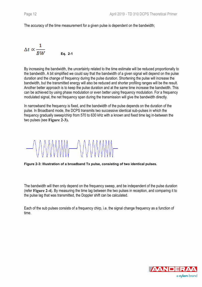
In narrowband the frequency is fixed, and the bandwidth of the pulse depends on the duration of the pulse. In Broadband mode, the DCPS transmits two successive identical sub-pulses in which the frequency gradually sweep/chirp from 570 to 630 kHz with a known and fixed time lag in-between the two pulses (see Figure 2-3).
Figure 2-3: Illustration of a broadband Tx pulse, consisting of two identical pulses.
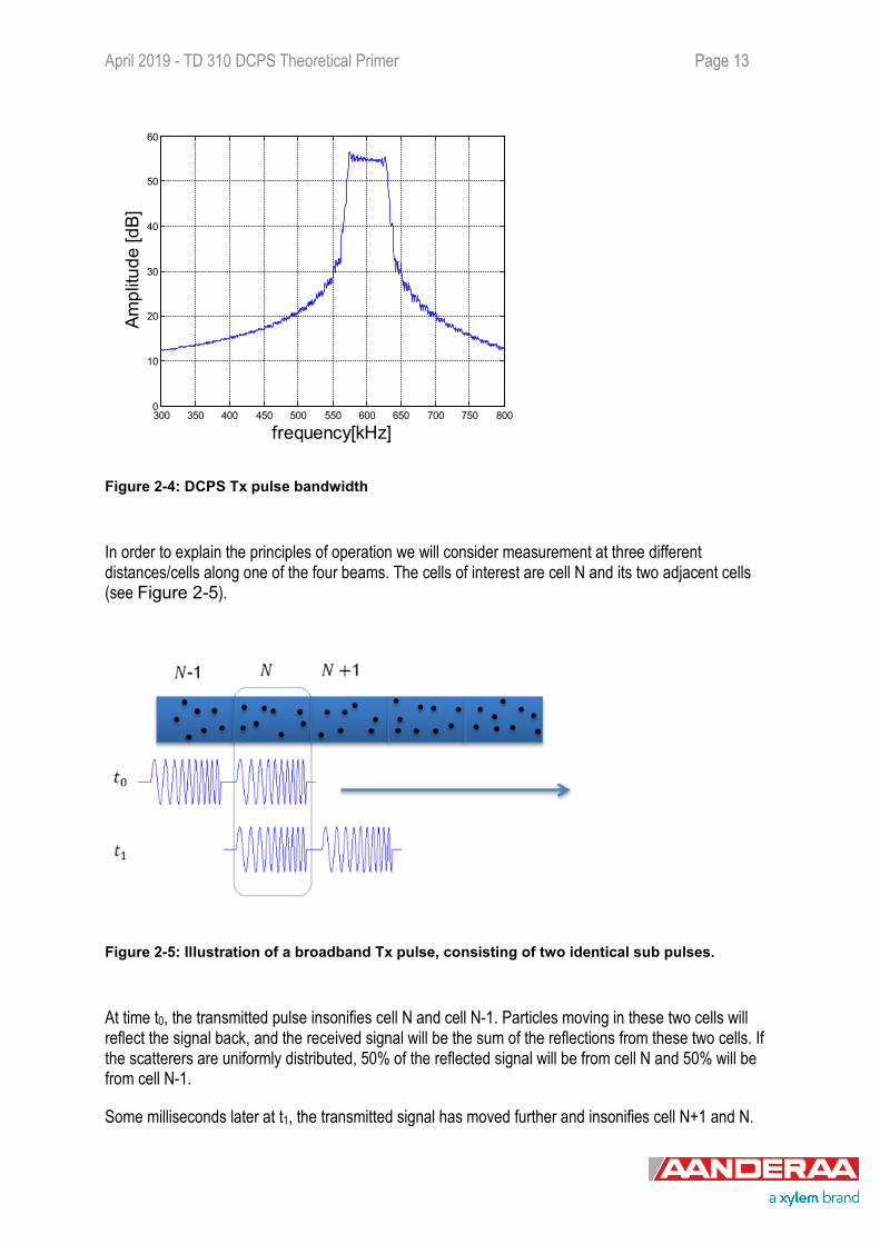
The bandwidth will then only depend on the frequency sweep, and be independent of the pulse duration (refer Figure 2-4). By measuring the time lag between the two pulses in reception, and comparing it to the pulse lag that was transmitted, the Doppler shift can be calculated.
Each of the sub pulses consists of a frequency chirp, i.e. the signal change frequency as a function of time.
April 2019 - TD 310 DCPS Theoretical Primer Page 13
Figure 2-4: DCPS Tx pulse bandwidth
In order to explain the principles of operation we will consider measurement at three different distances/cells along one of the four beams. The cells of interest are cell N and its two adjacent cells (see Figure 2-5).
Figure 2-5: Illustration of a broadband Tx pulse, consisting of two identical sub pulses.
At time t0, the transmitted pulse insonifies cell N and cell N-1. Particles moving in these two cells will reflect the signal back, and the received signal will be the sum of the reflections from these two cells. If the scatterers are uniformly distributed, 50% of the reflected signal will be from cell N and 50% will be from cell N-1.
Some milliseconds later at t1, the transmitted signal has moved further and insonifies cell N+1 and N.
300 350 400 450 500 550 600 650 700 750 8000
10
20
30
40
50
60
frequency[kHz]
Ampl
itude
[dB]
Page 14 April 2019 - TD 310 DCPS Theoretical Primer
Because the two sub pulses are identical, the reflected signal from cell N at t0 will be almost identical with the reflected signal from the same cell at t1. By finding the maximum correlation between the two received signals from each cell the time lag between the two pulses can be measured. This time lag will be modified if the particles are moving towards the instrument or away from it. If the time between the two sub pulses at the transmitter is called T0, and the change in lag from the reflected cell, compared to T0 is called Δt, the Doppler shift and current speed v can be calculated with Eq. 2-2 below.
Eq. 2-2
2.3.1 Correlation factor
By looking at we realize that the scatterer response from the first subpulse at t0 will be identical to the last subpulse at t1 if the scatterer remains the same at these two time instances. Likewise it will be sensible to assume that the response from the two remaining subpulses at t0 and t1 will be totally uncorrelated. If the scatterers are uniformly distributed, the scatterers stays within the cell and no noise is present, the correlation factor will be 0.5 reflecting a 50% correlation of the signal at t0 and t1. One could also argue that the signal is close to 100% correlated for 50% of the pulse, whereas the remaining 50% of the pulse is totally uncorrelated.
There are three main effect that will modify the correlation factor.
1) The signal to noise ratio will gradually be reduced with range . This will in turn reduce the part of the signal that is correlated as the noise at t0 and t1 will be uncorrelated. With added noise the correlated part of the signal will no longer be 100% correlated.
2) If the scatterers are not uniformly distributed the energy in the correlated part will no longer represent 50% of the total reflected energy. This will be the case when the signal hits an object or a boundary like the surface or bottom. The correlation factor will typically follow these transitions low-high-low when an object is reflecting the transmitted pulses.
3) In order for the correlated part to be 100% it will require the scatterers to remain identical for the time duration t1-t0. This can only be achieved in the case of 0 water current and the scatterers remains stationary. When the scatterers are exposed to current, some of the scatterers will move out of the cell, and some new scatterers will move in. Due to the short time duration t1-t0, the scatterers experience very little movement and the correlation factor for high SNR (Signal to Noise Ratio) cells are close to 0.5.
−
∆+= 1
2 0
0
tTTcv
April 2019 - TD 310 DCPS Theoretical Primer Page 15
smv
v beamhor /48.1
)sin(m==
θ
2.3.2 Ambiguity
The output of the correlation process is a phase value. When the Doppler shift is zero the phase is zero. When the Doppler shifts increase, so will the phase. A Doppler shift of approximately 1.25 m/s along the beam corresponds to a phase equal to 360 (360 = 0) which is exactly the same as for zero Doppler shift. For this reason the cross correlation process is not able to distinguish a Doppler shift of 1.5 from a Doppler shift of zero. In fact any Doppler shift outside the 1.25m/s range will be wrongly detected to be within the range 0 – 1.25 m/s.
This is called ambiguity and could hamper the correct operation of the instrument if not corrected for.
For a DCPS sensor in broadband mode, the center frequency is 600 kHz. One period of average frequency of 600 kHz corresponds to a period time of .1067.1 6
0 sT −⋅= By using Eq. 2-2 the ambiguity Doppler speed along the beam is calculated to be 1.25m/s.
Taking into account the orientation of the beams, θ=25 degrees off the vertical axis, the corresponding ambiguity horizontal speed will be:
Eq. 2-3
By allowing some tilt, a useful unambiguous speed of at least 1m/s will be achieved. The ambiguity lock function of the DCPS broadband mode can be used in order to lock the instrument in a horizontal current range, which is below 1m/s.
If the user is confident that the horizontal current will not exceed 1 m/s this configuration would be the preferred broadband configuration.
In case the ambiguity lock is not selected, several stages of ambiguity solving methods are automatically implemented in the DCPS in order to achieve a non-ambiguous solution.
These methods include:
Use of transmission pulses that are designed to give different ambiguity intervals. The combination of phase output from these set of pulses are unique for a limited number of intervals.
Remaining ambiguities are solved by putting consistency requirement on neighbouring cells in time and space and using statistics in order to resolve potential ambiguity.
Page 16 April 2019 - TD 310 DCPS Theoretical Primer
Compared to Narrowband, the Broadband mode gives a significant reduction in single ping standard deviation.
For example, for a 2m cell size, the equivalent single ping standard deviation is around 3 cm in broadband versus 20 cm in narrowband. The variation is reduced by the square root of the number of ping (accuracy improvement). In this example, the accuracy of one broadband ping would be equivalent to = 44 narrowband pings. On other words, to reach a similar standard deviation in narrowband as in broadband, the defined number of pings in narrowband would have to be 44 more than in broadband.
Even though the current consumption is higher per ping in broadband, the net power savings is significant using broadband compared to narrowband.
When the instrument is deployed in a buoy at the surface, the buoy will be affected by the surface dynamics which will highly influence the accuracy of the measurement. In general the buoy will remain stable but may experience some movement. In addition the surface current will also be influenced by the orbital movement due to surface waves. The duration of the transmitted pulse is in the order of 1ms, and the instrument movement during transmission may affect the measured current value.
So, if the instrument is moving due to waves or vibration, this movement can be looked upon as independent noise that will be added to the single ping standard deviation from the sensor itself.
Eq. 2-4
If we consider an example where the equivalent wave current noise is 20 cm/s, by using the above equation and assuming that the noise from the sensor is independent from the wave introduced noise, the ping accuracy would become:
Eq. 2-5
Eq. 2-6
By evaluating the accuracy of one BB ping versus one NB ping we see that this relation has been significantly changed; = 1.92 ping. The BB ping is still more effective in terms of accuracy per ping, but not in terms of accuracy per Wh of power consumption.
April 2019 - TD 310 DCPS Theoretical Primer Page 17
2.3.3 Limitation in the automatic ambiguity solution
The ambiguity resolving method incorporates use of two different Tx pulse sets each consisting of two sub pulses. In order to be able to resolve the ambiguity correctly, the 3D water current vector, as seen from the instrument should be fairly equal for two successive transmissions. If the instrument is exposed to movement during the measurement phase, this requirement would be violated and increase the probability of having unfiltered ambiguities in the detected current measurements. This could be the case if the instrument is installed on a surface platform exposed to heavy seas. Normal current fluctuations do not cause any problem to the ambiguity resolution algorithm. If horizontal current speed is expected to be above 1m/s and the instrument is expected to move around rapidly (as in buoy downward looking situation for example), narrowband mode is the preferred mode to be used.
2.3.4 From signal transmission to reception
Whether the instrument is configured in broadband or narrowband, the user needs to configure the number of cells and the cell size (from 0,5 to 5m).
The cell could be defined as the volume of water in which the instrument is performing the measurement.
By defining the cell size and the number of cells, and knowing the speed of sound, the instrument determines the time frame when the reflected signal from the corresponding cell will be received.
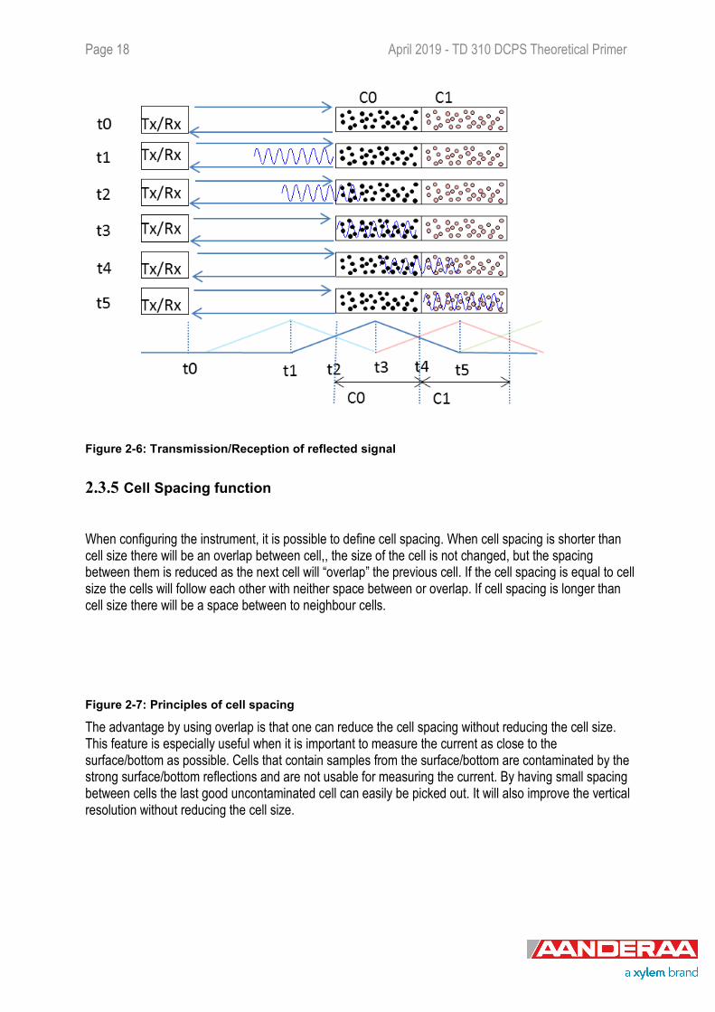
In the Figure 2-6, at t0, the sensors transmits the acoustic pulse. At the receiver the recording for the first cell (C0) starts when the center of the transmitted pulse reaches the beginning of C0 at t2, and stops when the center of the pulse leaves C0 at t4. In other words, the receiver collects samples for the same duration as the transmitted pulse. In Narrowband, the extent of the pulse in water also matches the cell size.
It will correspond to t1, when it reaches the second cell (cell1), it will correspond to t2, etc. The blanking zone is defined as the time needed for the transducer to shift from transmitting mode to receiving mode. For this reason the receiver will always start the measurement outside the blanking zone. The blanking zone is equivalent to 1 meter.
Page 18 April 2019 - TD 310 DCPS Theoretical Primer
Figure 2-6: Transmission/Reception of reflected signal
2.3.5 Cell Spacing function
When configuring the instrument, it is possible to define cell spacing. When cell spacing is shorter than cell size there will be an overlap between cell,, the size of the cell is not changed, but the spacing between them is reduced as the next cell will “overlap” the previous cell. If the cell spacing is equal to cell size the cells will follow each other with neither space between or overlap. If cell spacing is longer than cell size there will be a space between to neighbour cells.
Figure 2-7: Principles of cell spacing
The advantage by using overlap is that one can reduce the cell spacing without reducing the cell size. This feature is especially useful when it is important to measure the current as close to the surface/bottom as possible. Cells that contain samples from the surface/bottom are contaminated by the strong surface/bottom reflections and are not usable for measuring the current. By having small spacing between cells the last good uncontaminated cell can easily be picked out. It will also improve the vertical resolution without reducing the cell size.
April 2019 - TD 310 DCPS Theoretical Primer Page 19
2.3.6 Multiple columns - surface or instrument reference functions
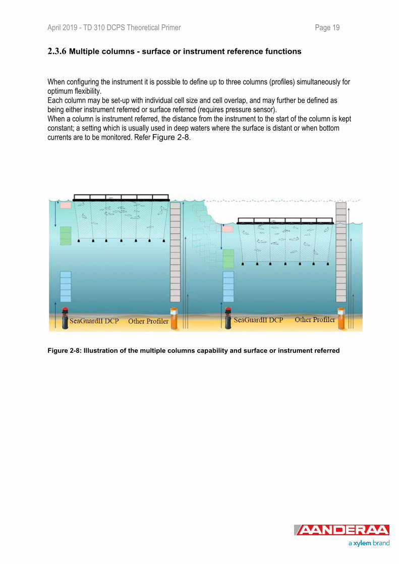
When configuring the instrument it is possible to define up to three columns (profiles) simultaneously for optimum flexibility. Each column may be set-up with individual cell size and cell overlap, and may further be defined as being either instrument referred or surface referred (requires pressure sensor). When a column is instrument referred, the distance from the instrument to the start of the column is kept constant; a setting which is usually used in deep waters where the surface is distant or when bottom currents are to be monitored. Refer Figure 2-8.
Figure 2-8: Illustration of the multiple columns capability and surface or instrument referred
Page 20 April 2019 - TD 310 DCPS Theoretical Primer
CHAPTER 3 Calculation of vertical and horizontal currents
3.1 Obtaining currents from multiple levels above/below the sensor
The four transducers transmit short pulses (pings) of acoustic energy into the water which are reflected against particles. By systematically clocking these reflections further and further away from the sensor and collecting their doppler shift, currents can be measured at multiple levels, up to 150 (divided over three columns; column 1: max 75 cells, column 2; max 50 cells and column 3 with 25 cells) simultaneously. For more information refer to the DCPS manual TD 304). An important factor in this context is knowing the speed of sound at the sensor which is obtained from an intergrated temperature sensor and assumed or measured salinity and pressure information. All instruments from Aanderaa have the option for plug-and play addition of smart-sensors for salinity, pressure and other parameters. It is possible to calculate the speed of sound “dynamically” so the sensor sends speed of sound changes based on values obtained from the sensors “continuously” to the DCPS sensor. In most cases for a sensor like the DCPS that has a maximum range of about 100 m in the best case, it is not important to know the full sound speed profile above/below. A strong stratification with large differences in sound speed could however have implications for at what distance from the instrument the cells are located. The DCPS sensor is operating at around 600 kHz which gives a typical range of 40-100 m depending on the scatter conditions. In general clear water with a low amount of particles gives shorter range and so do warm water. But also in situations where there is too much particles in the water (above 100 mg/l), like in a turbid river the range will be limited. For the Doppler current technique to be valid, some assumptions must be fulfilled:
1. The scatterers must drift with the water currents.
2. The water motions must be of a large scale compared to the separation of the beams (horizontal homogenity of the water).
3. The water motions must be of a large scale compared to the length of the transmitted pulse (vertical homogenity of the water).
The first assumption is critical since the movement of the scatterers in the water volume represents the water movement. It is essential that the scatterers do not move by themselves differently from the water current.
The other two assumtions are less critical.
April 2019 - TD 310 DCPS Theoretical Primer Page 21
3.1.1 Relationship between current measured at beams and earth referenced current.
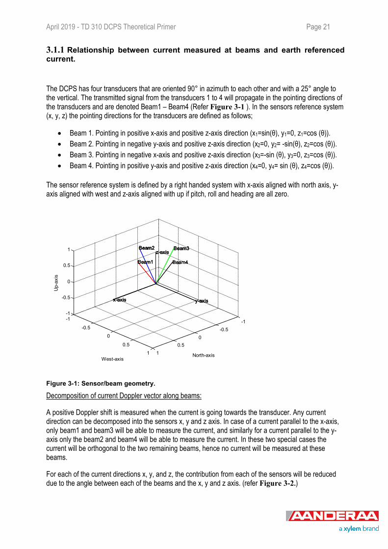
The DCPS has four transducers that are oriented 90° in azimuth to each other and with a 25° angle to the vertical. The transmitted signal from the transducers 1 to 4 will propagate in the pointing directions of the transducers and are denoted Beam1 – Beam4 (Refer Figure 3-1 ). In the sensors reference system (x, y, z) the pointing directions for the transducers are defined as follows;
• Beam 1. Pointing in positive x-axis and positive z-axis direction (x1=sin(θ), y1=0, z1=cos (θ)). • Beam 2. Pointing in negative y-axis and positive z-axis direction (x2=0, y2= -sin(θ), z2=cos (θ)). • Beam 3. Pointing in negative x-axis and positive z-axis direction (x3=-sin (θ), y3=0, z3=cos (θ)). • Beam 4. Pointing in positive y-axis and positive z-axis direction (x4=0, y4= sin (θ), z4=cos (θ)).
The sensor reference system is defined by a right handed system with x-axis aligned with north axis, y-axis aligned with west and z-axis aligned with up if pitch, roll and heading are all zero.
-1-0.5
00.5
1
-1
-0.5
0
0.5
1
-1
-0.5
0
0.5
1
y-axisy-axisy-axisy-axis
North-axis
Beam3 Beam3 Beam3 Beam3
Beam4 Beam4 Beam4 Beam4
z-axisz-axisz-axisz-axisBeam2 Beam2 Beam2 Beam2
Beam1 Beam1 Beam1 Beam1
West-axis
x-axisx-axisx-axisx-axis
Up-
axis
Figure 3-1: Sensor/beam geometry.
Decomposition of current Doppler vector along beams:
A positive Doppler shift is measured when the current is going towards the transducer. Any current direction can be decomposed into the sensors x, y and z axis. In case of a current parallel to the x-axis, only beam1 and beam3 will be able to measure the current, and similarly for a current parallel to the y-axis only the beam2 and beam4 will be able to measure the current. In these two special cases the current will be orthogonal to the two remaining beams, hence no current will be measured at these beams.
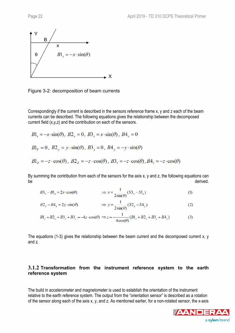
For each of the current directions x, y, and z, the contribution from each of the sensors will be reduced due to the angle between each of the beams and the x, y and z axis. (refer Figure 3-2.)
Page 22 April 2019 - TD 310 DCPS Theoretical Primer
Figure 3-2: decomposition of beam currents
Correspondingly if the current is described in the sensors reference frame x, y and z each of the beam currents can be described. The following equations gives the relationship between the decomposed current field (x,y,z) and the contribution on each of the sensors.
By summing the contribution from each of the sensors for the axis x, y and z, the following equations can be derived.
The equations (1-3) gives the relationship between the beam current and the decomposed current x, y and z.
3.1.2 Transformation from the instrument reference system to the earth reference system
The build in accelerometer and magnetometer is used to establish the orientation of the instrument relative to the earth reference system. The output from the “orientation sensor” is described as a rotation of the sensor along each of the axis x, y, and z. As mentioned earlier, for a non-rotated sensor, the x-axis
θ
B x
X
Y
)sin(1 θ⋅−= xB x
April 2019 - TD 310 DCPS Theoretical Primer Page 23
will be aligned with north, the y-axis will be aligned with west, and the z-axis will be aligned with up. A positive rotation around the x-axis corresponds to a positive roll value. A positive rotation around the y-axis corresponds to a negative pitch value, and finally a positive rotation around the z-axis corresponds to a negative value (counter clock rotation).
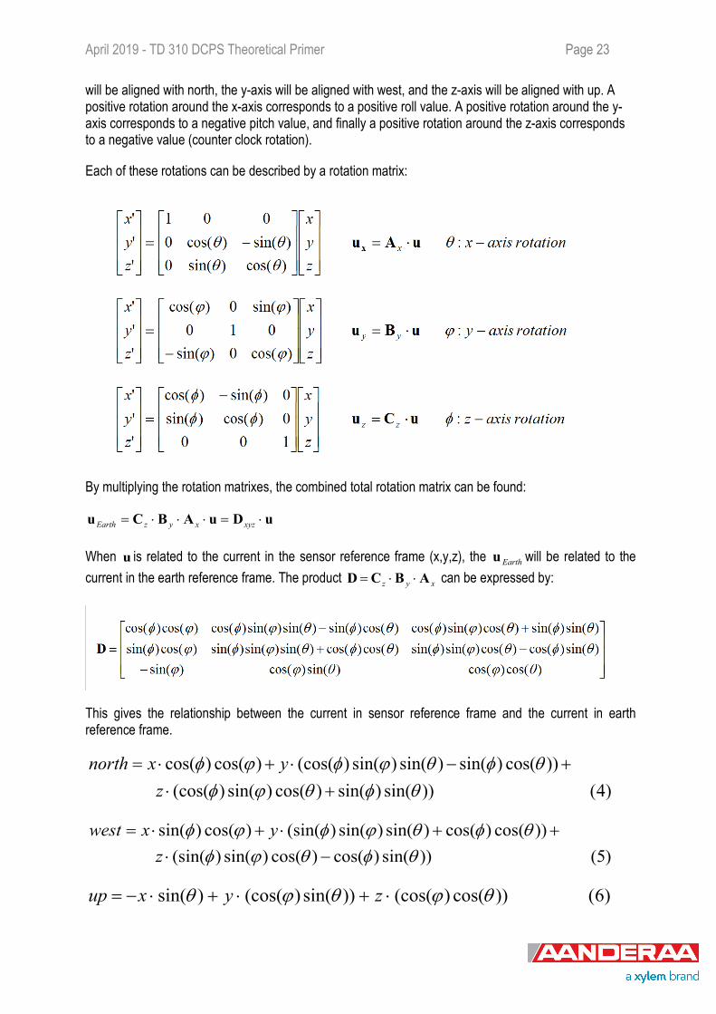
Each of these rotations can be described by a rotation matrix:
By multiplying the rotation matrixes, the combined total rotation matrix can be found:
uDuABCu ⋅=⋅⋅⋅= xyzxyzEarth
When u is related to the current in the sensor reference frame (x,y,z), the Earthu will be related to the current in the earth reference frame. The product xyz ABCD ⋅⋅= can be expressed by:
This gives the relationship between the current in sensor reference frame and the current in earth reference frame.
)4())sin()sin()cos()sin()(cos())cos()sin()sin()sin()(cos()cos()cos(
θφθϕφθφθϕφϕφ
+⋅+−⋅+⋅=
zyxnorth
)5())sin()cos()cos()sin()(sin())cos()cos()sin()sin()(sin()cos()sin(
θφθϕφθφθϕφϕφ
−⋅++⋅+⋅=
zyxwest
)6())cos()(cos())sin()(cos()sin( θϕθϕθ ⋅+⋅+⋅−= zyxup
Page 24 April 2019 - TD 310 DCPS Theoretical Primer
The combination of equation (1-3) and (4-6) gives the necessary equations in order to convert Doppler current measurement from the four beams into the current given in the earth coordinate reference frame for a given orientation of the sensor. The sensor orientation is measured for each ping. Within a record the current are averaged in the earth reference frame while utilizing the orientation measurement individually on a ping to ping basis.
At each depth level and for each of the four beams the total Doppler shift is obtained. To this both vertical and horizontal currents contribute but the contribution from the horizontal currents is normally larger because these currents are typically about 10 times stronger (unless there is strong up/down welling).
By using the descrived trigonometry, the current speed obtained from the Doppler shift given by each transducers is decomposed into positive or negative (moving towards or away from the transducer) currents in the X, Y and Z planes. By summing these up from the different beams and correcting for how the instrument was oriented with input from the compass and the accelerometer the speed and direction is calculated. After this calculation is done an adjustment for sound speed, fixed or measured, is implemented.
A minimum of 3 beams is needed to do these calculations but the DCPS has 4. In the DCPS the beams redundancy gives the possibility to calculate four 3-beam solutions and compare these with each other and with the 4-beam calculation. This is particularly useful if there are disturbing objects in one of the beams or if the circulation pattern is heterogeneous (described in Chapter 4-1).
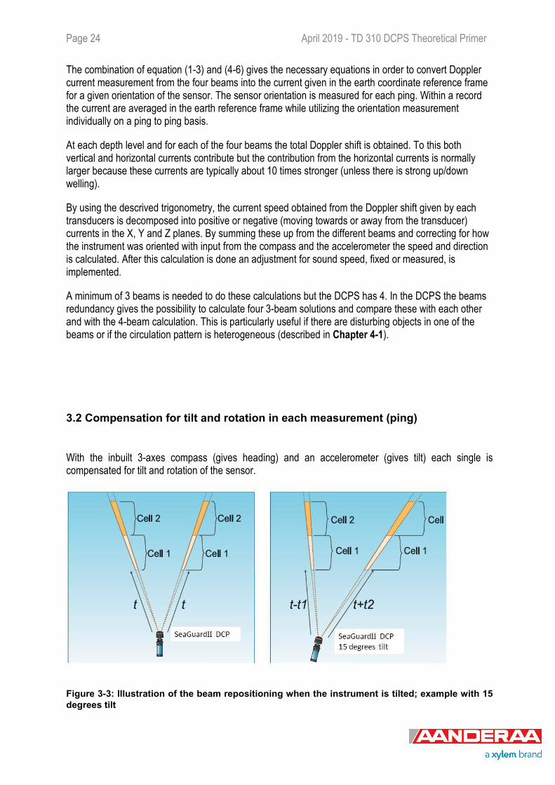
3.2 Compensation for tilt and rotation in each measurement (ping)
With the inbuilt 3-axes compass (gives heading) and an accelerometer (gives tilt) each single is compensated for tilt and rotation of the sensor.
Figure 3-3: Illustration of the beam repositioning when the instrument is tilted; example with 15 degrees tilt

April 2019 - TD 310 DCPS Theoretical Primer Page 25
Beam repositioning: refer Figure 3-3. When the sensor is tilting in one direction two of the beams will become more horizontally oriented and two more vertically oriented. The more vertically oriented beams will have a shorter travelling distance than the more horizontally oriented beams to reach the depth level / the cell at which the current will be measured. The DCPS will automatically tilt/time compensate the individual beams for each measurement so that the Doppler shift obtained for all the four beams will be obtained from the same depth level to obtain the true horizontal layer. The tilt compensation algorithm is updated for each ping and works with tilts up to ±50°. Above ±35°, the tilt sensor is outside the calibrated range. The profiling range and accuracy will decrease. For indication, at 50° tilt, the effective range will be 25m.
3.3 Surface current measurements
The DCPS, when upward looking, has the unique ability to measure the speed of the “boundary condition” that can be assimilated as the surface currents in the top cm layer (requires pressure data either using a pressure/tide/wave sensor sending data to the DCPS or mounted on the SeaGuardII equipped with pressure/tide/wave sensor). When it comes to the surface cell, the difference in impedance between the water and air creates an almost perfect reflector. The backscattered energy from the surface is normally extremely strong compared to the reflections from particles in the water and will totally dominate this cell. The pressure/wave/tide sensor is needed to determine when the strongest part of the reflection will be returned to the instrument and then the Doppler Shift for this reflection is calculated. Due to the strong reflection from the surface boundary layer it is possible to detect the surface cell at longer range (100 m) compared to ordinary cells. Wind generates capillary waves, and rapidly accelerates the surface boundary. For this reason there will be a strong correlation between both wind speed/surface boundary speed and wind direction/surface boundary direction.
Page 26 April 2019 - TD 310 DCPS Theoretical Primer
CHAPTER 4 The DCPS produces high quality data
4.1 Innovative three beam solution
The DCPS is equipped with unique software that makes it possible to obtain high quality current data even if one of the four beams is disturbed by for example an object. This can be useful in the case when for example one of the beams are receiving erroneous data caused by objects like mooring lines and floats that are not moving with the water flow. The DCPS has this ability built in. It gives enhanced possibilities to understand the prevailing conditions and obtain high quality data.
There are several ways to control the quality of the measurements. These are described in detail in the DCPS manual TD 304. Quality parameters include Acoustic Signal Strength (low signal indicate limit of reach), Standard Deviation of the current speed (high standard deviation can be caused by mixing/turbulence and when the signal strength is weak) and Cross Difference (for each depth the speed in beam 1 - speed beam 3 + speed beam 2 – speed beam 4 should be close to 0).
If the quality parameters indicate that the four beam solution are not consistent, perhaps due to an obstruction in one of the beams, the Auto Beam solution will use the three beam solution with the lowest single ping standard deviation to calculate the current speed. If the Cross Difference parameter indicates that the four-beam solution is consistent and of good quality, the Four-Beam solution will automatically be selected as the preferred Auto Beam solution. Thus, the four-beam solution is selected unless the Cross Difference of this solution is above a certain threshold.
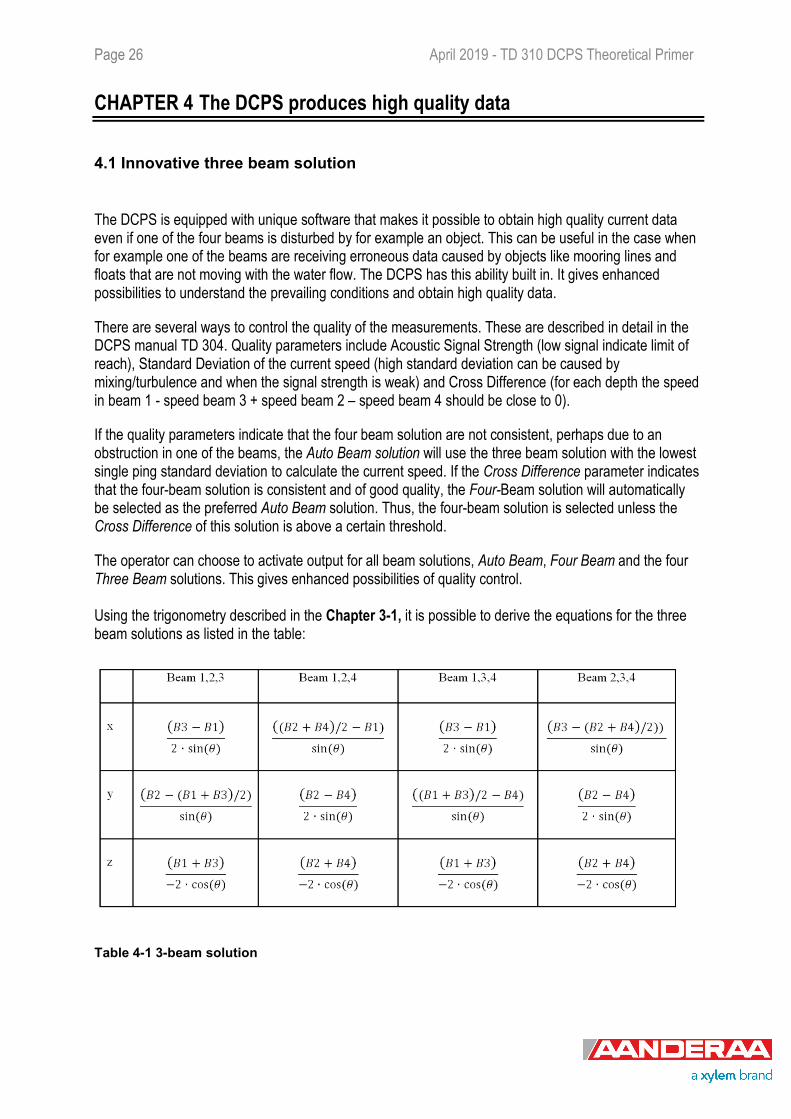
The operator can choose to activate output for all beam solutions, Auto Beam, Four Beam and the four Three Beam solutions. This gives enhanced possibilities of quality control. Using the trigonometry described in the Chapter 3-1, it is possible to derive the equations for the three beam solutions as listed in the table:
Table 4-1 3-beam solution
April 2019 - TD 310 DCPS Theoretical Primer Page 27
4.2 Calculating the noise levels/standard deviation
Depending on the mode, the DCPS transmits either a single tone burst or a broadband coded signal of duration Tp (refer CHAPTER 2 – Broadband principles of operation). The returned signal is compared to the transmitted pulse at a fixed time lag TL (correlation).
The weaker the correlation the noisier the data, which means less precision in the velocity estimate.
The standard deviation, σ, of an ensemble of pings is:
pLS NPDfA 1⋅
=σ Eq. 4-1
where Np is the number of pings, D is the cell size and PL is the pulselength. In narrowband, the pulselength is set equal to the cell size, whereas in broadband the pulselength is fixed. The constant, A, is dependent on the mode (broadband/narrowband), frequency, bandwidth, SNR (signal-to-noise ratio) and other properties related to the signal processing.
4.3 DCPS Narrowband internal processing –ARMA model
In Narrowband mode, the DCPS uses an Auto Regressive Moving Average (ARMA) model to estimate spectral properties of the backscattered signal.
The ARMA spectral estimation technique belongs to a family of spectral estimators called parametric models.
The motivation for using parametric models is the ability to achieve better power spectrum estimation than that produced by classical spectral estimators.
Page 28 April 2019 - TD 310 DCPS Theoretical Primer
CHAPTER 5 Limitations of Doppler Current Profilers
Physical and technical limitations of a Doppler Current Profiler are:
Precision in the estimation of the Doppler frequency. Influence of acoustic side lobes. Measurement range. Blanking distance. Random and systematic errors.
The precision in the estimation of the Doppler frequency has been discussed previously. The other limitations are discussed in this chapter.
5.1 Influence of acoustic side lobes and the contaminated zone close to surface/bottom
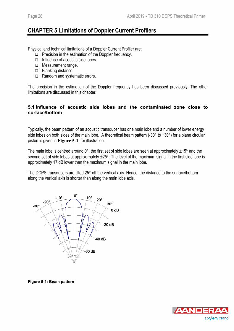
Typically, the beam pattern of an acoustic transducer has one main lobe and a number of lower energy side lobes on both sides of the main lobe. A theoretical beam pattern (-30° to +30°) for a plane circular piston is given in Figure 5-1, for illustration.
The main lobe is centred around 0°, the first set of side lobes are seen at approximately ±15° and the second set of side lobes at approximately ±25°. The level of the maximum signal in the first side lobe is approximately 17 dB lower than the maximum signal in the main lobe.
The DCPS transducers are tilted 25° off the vertical axis. Hence, the distance to the surface/bottom along the vertical axis is shorter than along the main lobe axis.
Figure 5-1: Beam pattern
-60 dB
-40 dB
-20 dB
0°
0 dB
10° 20°30°
-10°-20°
-30°
-60 dB
-40 dB
-20 dB
0°
0 dB
10° 20°30°
-10°-20°
-30°
April 2019 - TD 310 DCPS Theoretical Primer Page 29
As a result, strong signals backscattered off the surface/bottom originating from the side lobes that arrive at the same time as the backscattered signal from the main lobe will “acoustically contaminate” measurements close to boundaries like the surface (upward looking) and the bottom (downward looking). The contaminated zone depends of the deployment depth (when upward looking) or water depth (if instrument is downward looking) and the pulse length (the pulse length is approximately 1m in broadband and is equal to the cell size in narrowband). Please observe that surface current measurements, described in chapter 3-3, are not affected by the side lobe contamination.
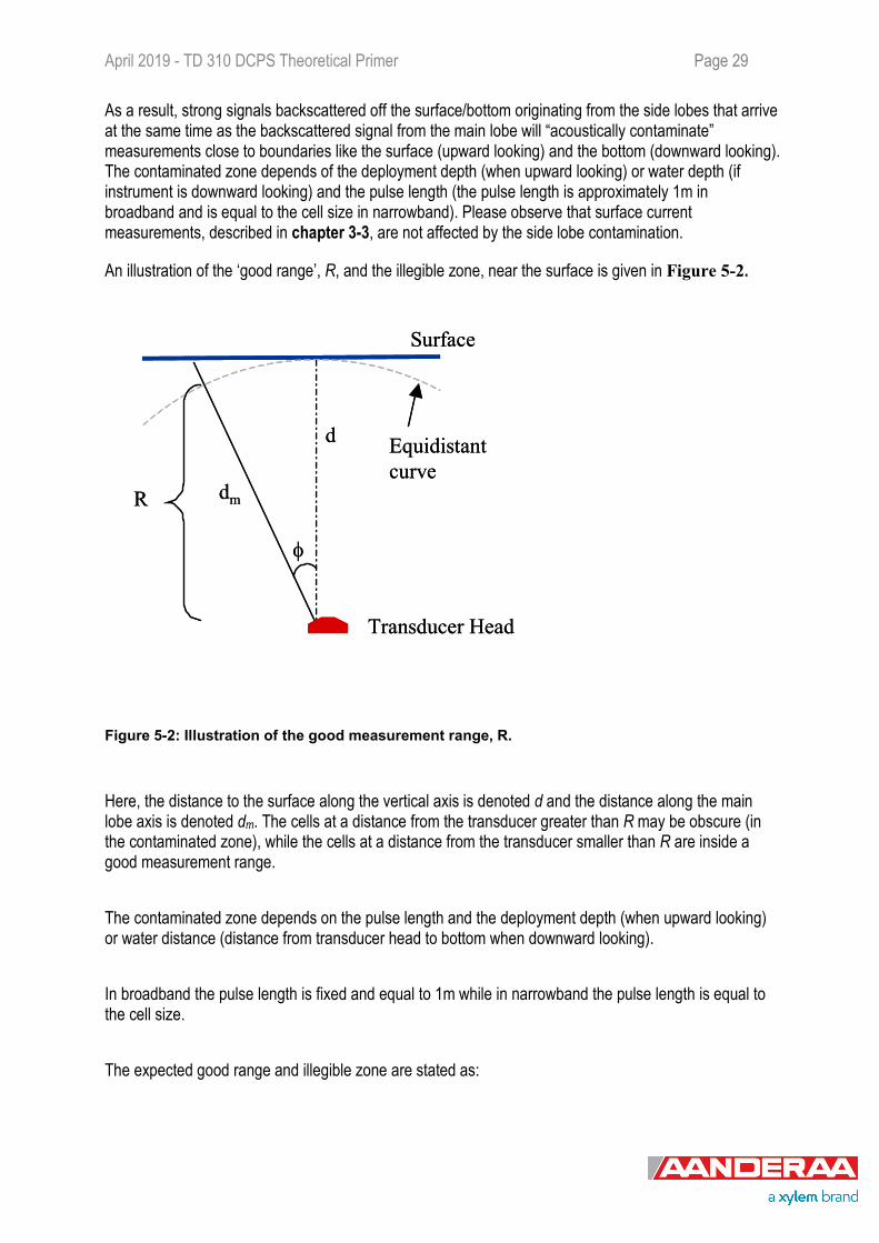
An illustration of the ‘good range’, R, and the illegible zone, near the surface is given in Figure 5-2.
Figure 5-2: Illustration of the good measurement range, R.
Here, the distance to the surface along the vertical axis is denoted d and the distance along the main lobe axis is denoted dm. The cells at a distance from the transducer greater than R may be obscure (in the contaminated zone), while the cells at a distance from the transducer smaller than R are inside a good measurement range.
The contaminated zone depends on the pulse length and the deployment depth (when upward looking) or water distance (distance from transducer head to bottom when downward looking).
In broadband the pulse length is fixed and equal to 1m while in narrowband the pulse length is equal to the cell size.
The expected good range and illegible zone are stated as:
dmR
Transducer Head
Surface
d Equidistantcurve
φ
dmR
Transducer Head
Surface
d Equidistantcurve
φ
Page 30 April 2019 - TD 310 DCPS Theoretical Primer
( ) xdR −⋅= φcos Eq. 5-1
( ) xdRdI +−=−= )cos1( φ Eq. 5-2
where d is the vertical distance from the transducers to the surface and is the beam angle relative to the vertical, if broadband is used; , where p is the pulselength; x is half the pulselength but in broadband two pulses are sent after each other so x=1m as the pulse length is always 1m in broadband. Thus, for a 25° beam angle with no additional instrument tilt, 20m depth for example, a pulse length of 1m in broadband, the illegible zone would be 2,9m. If the column is defined as surface referred, it should not start closer than 2,9m from the surface. If the column is instrument referred and the cell closest to the surface is inside the contaminated zone then it would have to be discarded.
If narrowband is used , p is the pulse length/cell size so x becomes half of the cell size. If the cell size is 1m, the instrument 20m depth, the contaminated zone would become 2,4m.
5.2 Total measurement range
The total measurement range depends on the source level i.e. the transmitted power, the transducer efficiency and the frequency. At 600 kHz, the transducers are relatively small and their efficiency is limited by non-linear behavior and cavitation. Hence for linear wave propagation, the transmitted power of a small transducer is limited. An increased pulse length may increase the range by a small amount.
Field data has demonstrated that the DCPS has an approximate range of 40-100 m depending on the scattering conditions. The range is similar using broadband and narrowband.
5.3 Blanking distance closest to the instrument
After transmitting an acoustic pulse, the transducers and electronics must rest a short time for the transducers to stop vibrating (ringing) before it is able to act as a microphone and receive the very weak (compared to the transmitted pulse) reflected acoustic signals.
The ringing of the transducers depends on transducer size, frequency and the material embedding the transducers.
About half a millisecond of ringing corresponds to a 1 m blanking distance assuming a sound speed in water of 1500 m/s.
April 2019 - TD 310 DCPS Theoretical Primer Page 31
5.4 Random and systematic errors
Two types of errors contribute to velocity uncertainty; random and systematic (bias) errors. Random errors can be averaged out while systematic errors cannot.
Random errors are reduced by the square root of the number of samples in one record.
Random errors depend on a number of factors:
Pulse Length: The shorter the pulse length, the greater the random error for a given frequency.
Transmit Frequency: The lower the frequency, the greater the random error for a given pulse length.
SNR: The lower the signal-to-noise ratio, the greater the random error.
Bias errors are non-random and can therefore not be reduced by data averaging. Fortunately, these errors are in general small, typically ~0.5 cm/s. The expression for the standard deviation is already shown in Eq. 4-1.
5.4.1 Beam separation
The separation of the 4 transducer beams poses a limit to the vertical and horizontal scales of motion that can be resolved. With increasing distance from the transducer the sampling volume (cell volume) and the distance between the 4 cells at the same distance from the transducer increase. Thus, a short period velocity fluctuation resolved in close range may not be resolved in the end of range where the horizontal distance between the cells is greater.
5.4.2 Echo intensity and backscatters
A 600 kHz transducer transmits sound waves with a wavelength of a couple of millimeters. These waves may bounce off small planktons, particles or air-bubbles that have an acoustic impedance difference to the medium itself; the water. Bubbles, however, are compressible and take energy from the sound waves and thus often limit the range. Bubble clouds exist e.g. in the surface wave break zone or in the wake of ships.
In oceanographic applications the main limitation for obtaining good data at a distance from the sensor is poor backscatter. If the scatterers are comprised of large zooplankton moving independently of the water current, a very critical assumption is violated and data may be obscured.
If the scatterers are too few the backscattered energy is low and self-noise may corrupt the signal. The backscattered energy, or the Echo Intensity, is measured by the instrument relative to the maximum intensity.
Page 32 April 2019 - TD 310 DCPS Theoretical Primer
Echo intensity can be used not only as a quality parameter but also to record temporal and spatial relative abundance of plankton, particles and/or bubbles. The Sonar equation has to be employed and biological ‘ground proof’ needs to be taken.
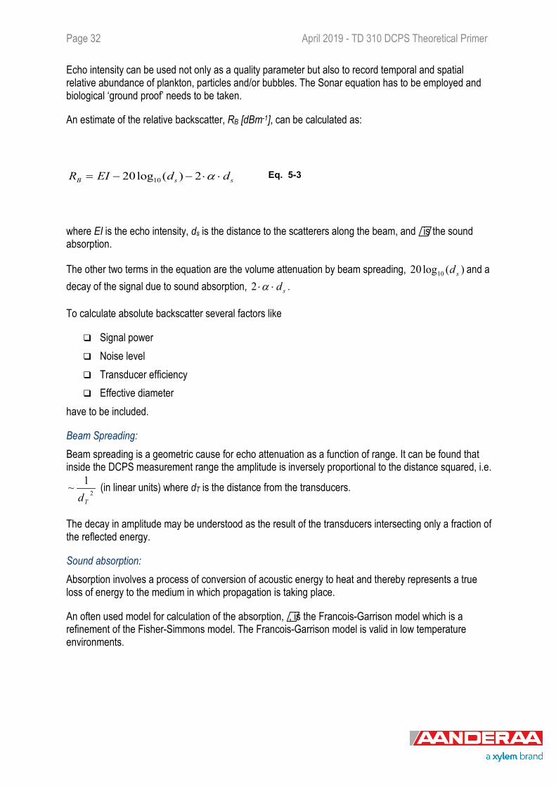
An estimate of the relative backscatter, RB [dBm-1], can be calculated as:
ssB ddEIR ⋅⋅−−= α2)(log20 10 Eq. 5-3
where EI is the echo intensity, ds is the distance to the scatterers along the beam, and is the sound absorption.
The other two terms in the equation are the volume attenuation by beam spreading, )(log20 10 sd and a decay of the signal due to sound absorption, sd⋅⋅α2 .
To calculate absolute backscatter several factors like
Signal power Noise level Transducer efficiency Effective diameter
have to be included.
Beam Spreading: Beam spreading is a geometric cause for echo attenuation as a function of range. It can be found that inside the DCPS measurement range the amplitude is inversely proportional to the distance squared, i.e.
2
1~Td
(in linear units) where dT is the distance from the transducers.
The decay in amplitude may be understood as the result of the transducers intersecting only a fraction of the reflected energy.
Sound absorption: Absorption involves a process of conversion of acoustic energy to heat and thereby represents a true loss of energy to the medium in which propagation is taking place.
An often used model for calculation of the absorption, , is the Francois-Garrison model which is a refinement of the Fisher-Simmons model. The Francois-Garrison model is valid in low temperature environments.
April 2019 - TD 310 DCPS Theoretical Primer Page 33
CHAPTER 6 Acoustic Waves
6.1 Waves explained
Waves are moving energy traveling along the interface between ocean and atmosphere. Most of the waves are generated by wind blowing across the surface; wind blows over the water surface and generate capillary waves. Once capillary waves are created, the friction from the turbulent air on the water surface increases and the energy transport from wind to waves will increase. As more energy is transferred to the ocean, gravity waves develop. Because they reach greater height at this stage, gravity replaces capillarity given these waves their name. Once a wave accumulates enough energy and grows to a certain size it will bump into the wave in front of it which will cause it to gain height. By gaining height a wave exposes its surface to more wind and gains more energy. This cycle continues producing larger waves as long as the wind blows in the same direction. The transferred energy from wind to waves depends on the wind field. The wind field is characterized by the wind speed, wind duration and the fetch (the fetch is the length of water over which the wind has blown). The longer the fetch and the faster the wind speed, the more energy is imparted to the water surface and the larger the resulting sea state (size of the waves) will be. This area where wind-driven waves are generated is called “sea” or the sea area.
As waves generated in a sea area move towards its margins, wind speeds diminish and the wave eventually move faster than the wind. When this occurs, wave steepness decreases and they become long-crested waves called swells. Swells are uniform, symmetrical waves that have traveled out of the area where they originated. Swells moves with little loss of energy over large stretches of the ocean surface, transporting energy away from one sea area and depositing it in another. Thus there can be waves at distant shorelines where there is no wind.
Waves with longer wavelengths travel faster and thus leave the sea area first. They are followed by slower, shorter wave trains or groups of waves. The progression from long, fast waves to short, slow waves illustrates the principle of wave dispersion – the sorting of waves by their wavelength. Waves of many wavelengths are present in the generating area.
When swells from different storms run together the water clash or interfere with one another, giving rise to interference patterns. An interference pattern produced when two or more wave systems collide is the sum of the disturbance that each wave would have produced individually. The combined swells consist of waves of various heights and lengths that develop into a complex mixed interference pattern, which explains the varied sequence of high and lower wave and other irregular wave patterns that occur when swell approaches the seashore. In the open ocean, several swell systems often interact creating complex wave patterns and sometimes large waves that can be hazardous to ships.
Waves are energy in motion. Waves transmit energy by means of cyclic movement through matter. The medium itself does not travel in the direction of the energy that is passing through it. The movement of particles at the ocean surface move in circular orbits referred to as circular orbital motion.
Page 34 April 2019 - TD 310 DCPS Theoretical Primer
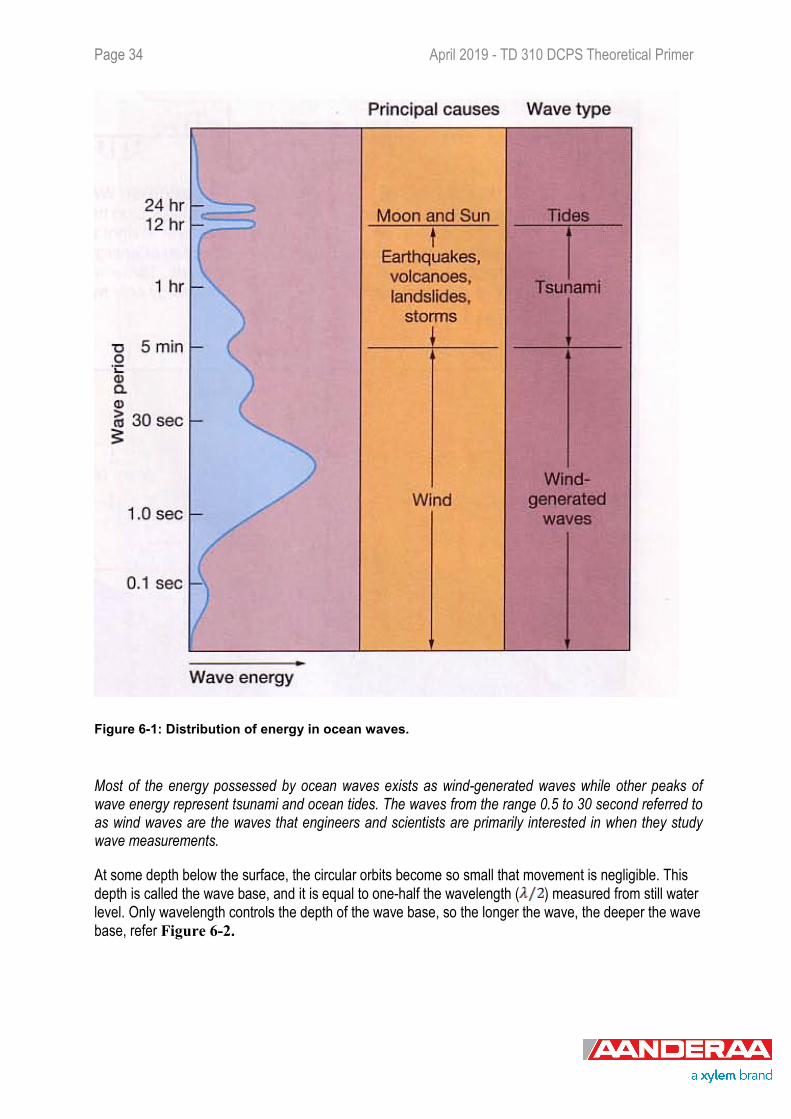
Figure 6-1: Distribution of energy in ocean waves.
Most of the energy possessed by ocean waves exists as wind-generated waves while other peaks of wave energy represent tsunami and ocean tides. The waves from the range 0.5 to 30 second referred to as wind waves are the waves that engineers and scientists are primarily interested in when they study wave measurements.
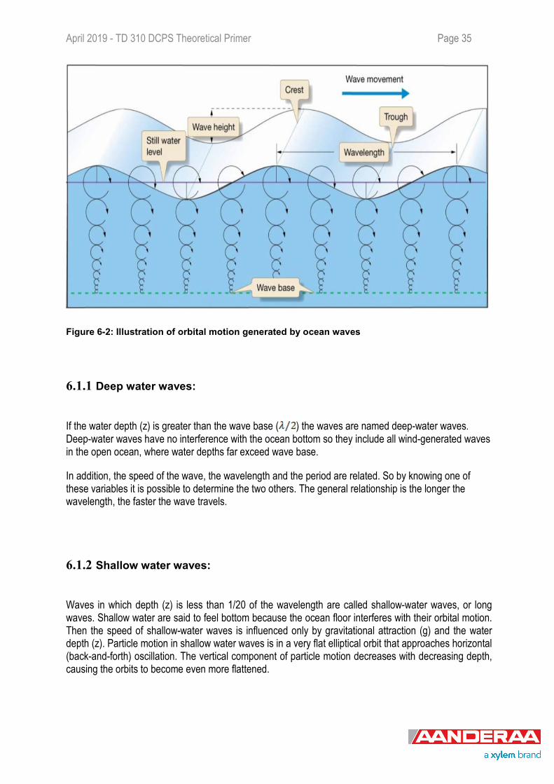
At some depth below the surface, the circular orbits become so small that movement is negligible. This depth is called the wave base, and it is equal to one-half the wavelength ( ) measured from still water level. Only wavelength controls the depth of the wave base, so the longer the wave, the deeper the wave base, refer Figure 6-2.
April 2019 - TD 310 DCPS Theoretical Primer Page 35
Figure 6-2: Illustration of orbital motion generated by ocean waves
6.1.1 Deep water waves:
If the water depth (z) is greater than the wave base ( ) the waves are named deep-water waves. Deep-water waves have no interference with the ocean bottom so they include all wind-generated waves in the open ocean, where water depths far exceed wave base.
In addition, the speed of the wave, the wavelength and the period are related. So by knowing one of these variables it is possible to determine the two others. The general relationship is the longer the wavelength, the faster the wave travels.
6.1.2 Shallow water waves:
Waves in which depth (z) is less than 1/20 of the wavelength are called shallow-water waves, or long waves. Shallow water are said to feel bottom because the ocean floor interferes with their orbital motion. Then the speed of shallow-water waves is influenced only by gravitational attraction (g) and the water depth (z). Particle motion in shallow water waves is in a very flat elliptical orbit that approaches horizontal (back-and-forth) oscillation. The vertical component of particle motion decreases with decreasing depth, causing the orbits to become even more flattened.

Page 36 April 2019 - TD 310 DCPS Theoretical Primer
As deep-water waves of swell move toward continental margins over gradually shoaling (shoal = shallow) water, they eventually encounter water depths that are less than one-half of their wavelength and become transitional waves. Actually, any shallowly submerged obstacle (such a coral reef, sunken wreck or sand bar) will cause waves to release some energy.
Many physical changes occur to a wave as it encounters shallow water, becomes a shallow-water wave and breaks. The shoaling depths interfere with water particle movement at the base of the wave so the wave speed decreases. As one wave slows, the following waveform, which is still moving at its original speed, moves closer to the wave that is being slowed causing a decrease in wavelength. The energy in the wave, which remains the same, must go somewhere so wave height increases. This increase in wave height combined with the decrease in wavelength causes an increase in wave steepness (H/L). When the wave steepness reaches the 1:7 ratio, the waves break as surf, refer to Figure 6-3.
Figure 6-3: Wave steepness increase
As waves approach the shore and encounter water depths of less than one-half wavelength, the waves feel bottom. The wave speed decreases and waves stickup against the shore, causing the wavelength to decrease. This results in an increase in wave height to the point where the wave steepness is increased beyond the 1:7 ratio, causing the wave to pitch forward and break in the surf zone.
April 2019 - TD 310 DCPS Theoretical Primer Page 37
CHAPTER 7 Measuring waves with an Acoustic Doppler Profiler
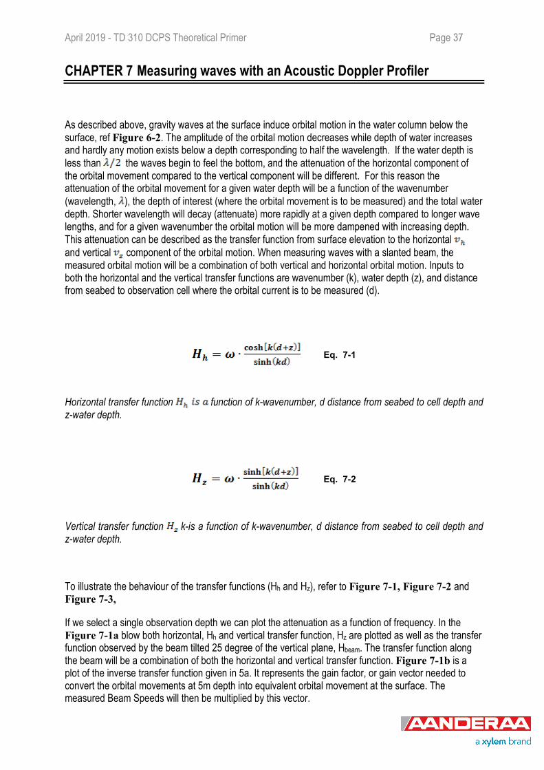
As described above, gravity waves at the surface induce orbital motion in the water column below the surface, ref Figure 6-2. The amplitude of the orbital motion decreases while depth of water increases and hardly any motion exists below a depth corresponding to half the wavelength. If the water depth is less than the waves begin to feel the bottom, and the attenuation of the horizontal component of the orbital movement compared to the vertical component will be different. For this reason the attenuation of the orbital movement for a given water depth will be a function of the wavenumber (wavelength, ), the depth of interest (where the orbital movement is to be measured) and the total water depth. Shorter wavelength will decay (attenuate) more rapidly at a given depth compared to longer wave lengths, and for a given wavenumber the orbital motion will be more dampened with increasing depth. This attenuation can be described as the transfer function from surface elevation to the horizontal and vertical component of the orbital motion. When measuring waves with a slanted beam, the measured orbital motion will be a combination of both vertical and horizontal orbital motion. Inputs to both the horizontal and the vertical transfer functions are wavenumber (k), water depth (z), and distance from seabed to observation cell where the orbital current is to be measured (d).
Eq. 7-1
Horizontal transfer function function of k-wavenumber, d distance from seabed to cell depth and z-water depth.
Eq. 7-2
Vertical transfer function k-is a function of k-wavenumber, d distance from seabed to cell depth and z-water depth.
To illustrate the behaviour of the transfer functions (Hh and Hz), refer to Figure 7-1, Figure 7-2 and Figure 7-3,
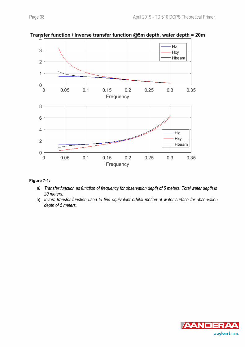
If we select a single observation depth we can plot the attenuation as a function of frequency. In the Figure 7-1a blow both horizontal, Hh and vertical transfer function, Hz are plotted as well as the transfer function observed by the beam tilted 25 degree of the vertical plane, Hbeam. The transfer function along the beam will be a combination of both the horizontal and vertical transfer function. Figure 7-1b is a plot of the inverse transfer function given in 5a. It represents the gain factor, or gain vector needed to convert the orbital movements at 5m depth into equivalent orbital movement at the surface. The measured Beam Speeds will then be multiplied by this vector.
Page 38 April 2019 - TD 310 DCPS Theoretical Primer
Figure 7-1:
a) Transfer function as function of frequency for observation depth of 5 meters. Total water depth is 20 meters.
b) Invers transfer function used to find equivalent orbital motion at water surface for observation depth of 5 meters.
April 2019 - TD 310 DCPS Theoretical Primer Page 39
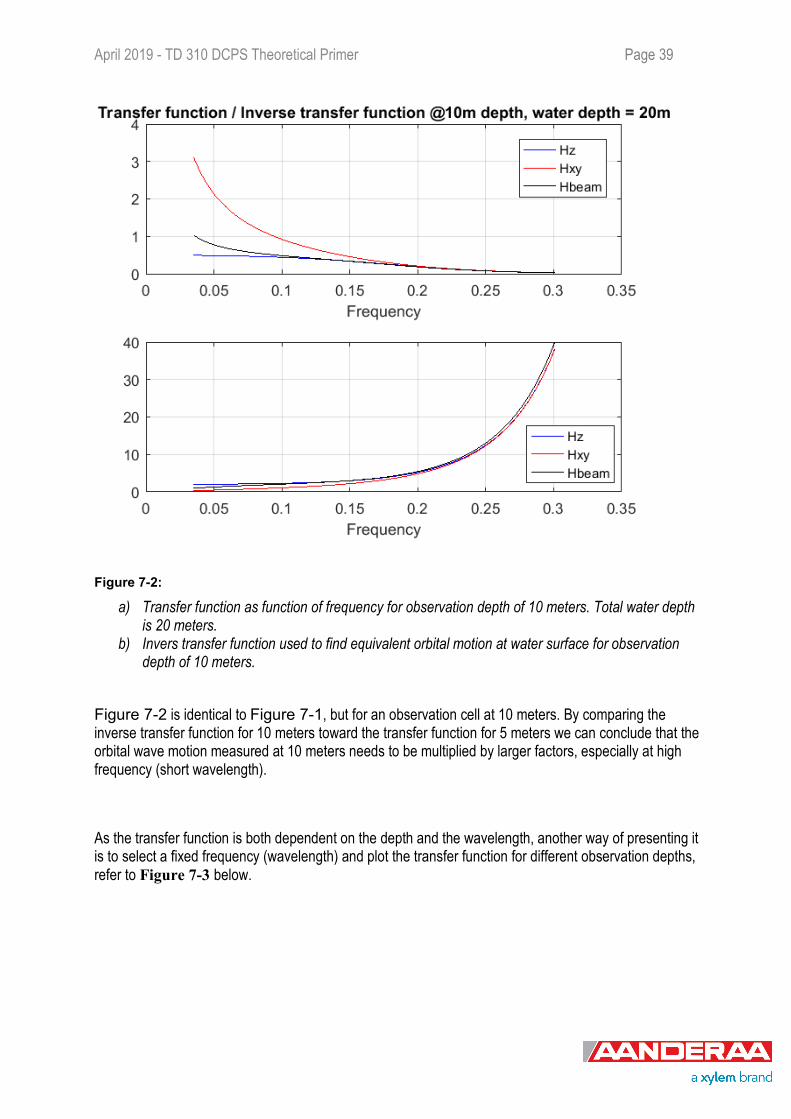
Figure 7-2:
a) Transfer function as function of frequency for observation depth of 10 meters. Total water depth is 20 meters.
b) Invers transfer function used to find equivalent orbital motion at water surface for observation depth of 10 meters.
Figure 7-2 is identical to Figure 7-1, but for an observation cell at 10 meters. By comparing the inverse transfer function for 10 meters toward the transfer function for 5 meters we can conclude that the orbital wave motion measured at 10 meters needs to be multiplied by larger factors, especially at high frequency (short wavelength).
As the transfer function is both dependent on the depth and the wavelength, another way of presenting it is to select a fixed frequency (wavelength) and plot the transfer function for different observation depths, refer to Figure 7-3 below.
Page 40 April 2019 - TD 310 DCPS Theoretical Primer
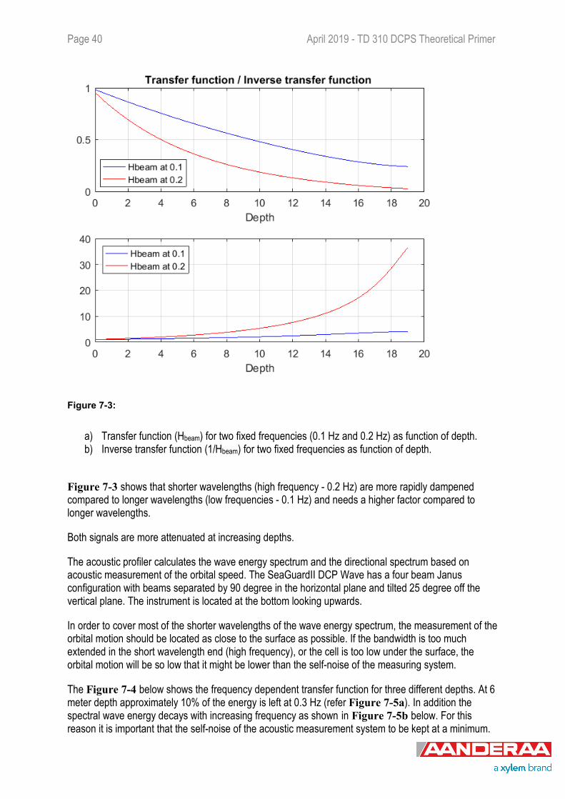
Figure 7-3:
a) Transfer function (Hbeam) for two fixed frequencies (0.1 Hz and 0.2 Hz) as function of depth. b) Inverse transfer function (1/Hbeam) for two fixed frequencies as function of depth.
Figure 7-3 shows that shorter wavelengths (high frequency - 0.2 Hz) are more rapidly dampened compared to longer wavelengths (low frequencies - 0.1 Hz) and needs a higher factor compared to longer wavelengths.
Both signals are more attenuated at increasing depths.
The acoustic profiler calculates the wave energy spectrum and the directional spectrum based on acoustic measurement of the orbital speed. The SeaGuardII DCP Wave has a four beam Janus configuration with beams separated by 90 degree in the horizontal plane and tilted 25 degree off the vertical plane. The instrument is located at the bottom looking upwards.
In order to cover most of the shorter wavelengths of the wave energy spectrum, the measurement of the orbital motion should be located as close to the surface as possible. If the bandwidth is too much extended in the short wavelength end (high frequency), or the cell is too low under the surface, the orbital motion will be so low that it might be lower than the self-noise of the measuring system.
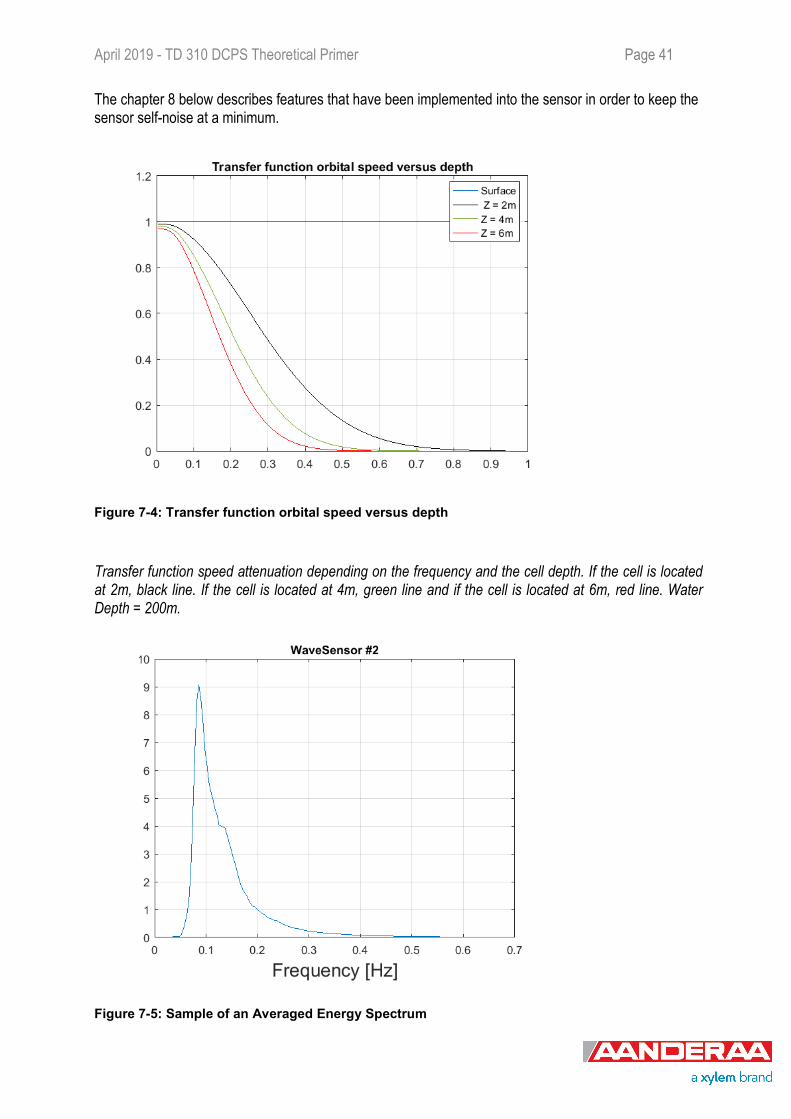
The Figure 7-4 below shows the frequency dependent transfer function for three different depths. At 6 meter depth approximately 10% of the energy is left at 0.3 Hz (refer Figure 7-5a). In addition the spectral wave energy decays with increasing frequency as shown in Figure 7-5b below. For this reason it is important that the self-noise of the acoustic measurement system to be kept at a minimum.
April 2019 - TD 310 DCPS Theoretical Primer Page 41
The chapter 8 below describes features that have been implemented into the sensor in order to keep the sensor self-noise at a minimum.
Figure 7-4: Transfer function orbital speed versus depth
Transfer function speed attenuation depending on the frequency and the cell depth. If the cell is located at 2m, black line. If the cell is located at 4m, green line and if the cell is located at 6m, red line. Water Depth = 200m.
Figure 7-5: Sample of an Averaged Energy Spectrum
Page 42 April 2019 - TD 310 DCPS Theoretical Primer
CHAPTER 8 Adaptive transmission pulse to optimize the wave measurement accuracy
8.1 Sensor self-noise In order to maximize the measured bandwidth, the sensor self-noise should be kept low. For an acoustic profiler the self-noise can be described in terms of single ping standard deviation. The SeaGuardII DCP Wave can operate both in Narrowband and Broadband. The broadband mode of the SeaGuardII DCP Wave utilizes a dual Hyperbolic Frequency Modulation (HFM/Chirp) ensuring that the bandwidth of the transmission pulse matches the bandwidth of the transducer. The transmission pulse has been extended to a 20% bandwidth, improving the signal to noise ratio. The advantage of using the HFM broadband pulse compared to a sequence of coded pulses is that the available bandwidth of the measurement can be optimized by adjusting the sweep independent of the Tx pulse length. As a result the transition region is very sharp with little energy leakage outside the band of interest. The HFM pulse also gives minimal correlation-loss for a Doppler shifted signal. In case the broadband pulse is build up by a sequence of coded pulses, the lag is adjusted by modifying the number of coded sequences.
Three different factors define the accuracy of the measurement.
1) The bandwidth of the system, ie. Tx band, Rx band and bandwidth used in the processing chain. Broader bandwidth gives a narrower matched filter response and a more accurate phase estimate used in the Doppler processing.
2) The time duration of the transmitted signal. A longer TX pulse gives a longer average time and better Doppler estimate.
3) The lag between the transmitted sub-pulses has a great impact on the accuracy and the maximum Doppler shift that can be measured. By increasing the lag the single ping standard deviation will be improved, but the useful range of Doppler speeds that can be read unambiguously will be reduced.
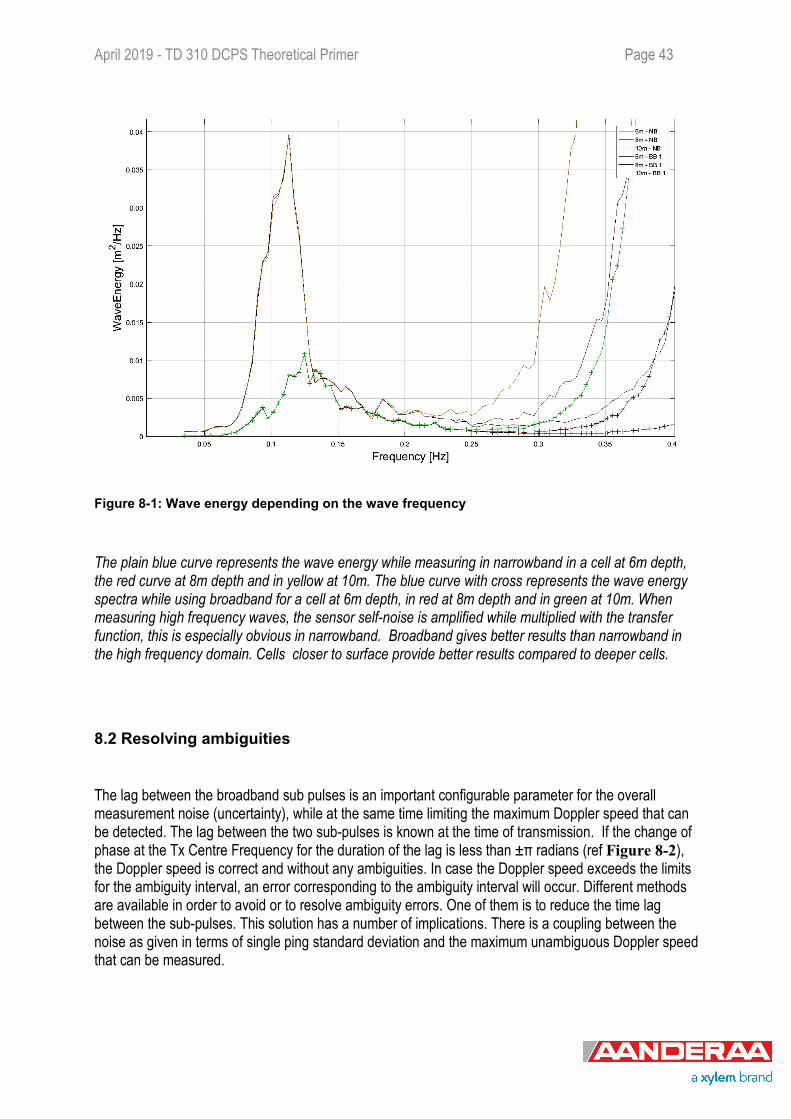
The benefits of utilizing broadband can be seen in Figure 8-1. When using broadband the single ping standard deviation is significantly lower compared to narrowband. The result is reduced sensor self-noise, and can be observed as reduced (noise) energy at higher frequencies. Due to less attenuation of the wave orbital motion at cells closer to the surface the selected cell should be as close to the surface as possible without coming in the side lobes contaminated surface layer.
April 2019 - TD 310 DCPS Theoretical Primer Page 43
Figure 8-1: Wave energy depending on the wave frequency
The plain blue curve represents the wave energy while measuring in narrowband in a cell at 6m depth, the red curve at 8m depth and in yellow at 10m. The blue curve with cross represents the wave energy spectra while using broadband for a cell at 6m depth, in red at 8m depth and in green at 10m. When measuring high frequency waves, the sensor self-noise is amplified while multiplied with the transfer function, this is especially obvious in narrowband. Broadband gives better results than narrowband in the high frequency domain. Cells closer to surface provide better results compared to deeper cells.
8.2 Resolving ambiguities
The lag between the broadband sub pulses is an important configurable parameter for the overall measurement noise (uncertainty), while at the same time limiting the maximum Doppler speed that can be detected. The lag between the two sub-pulses is known at the time of transmission. If the change of phase at the Tx Centre Frequency for the duration of the lag is less than ±π radians (ref Figure 8-2), the Doppler speed is correct and without any ambiguities. In case the Doppler speed exceeds the limits for the ambiguity interval, an error corresponding to the ambiguity interval will occur. Different methods are available in order to avoid or to resolve ambiguity errors. One of them is to reduce the time lag between the sub-pulses. This solution has a number of implications. There is a coupling between the noise as given in terms of single ping standard deviation and the maximum unambiguous Doppler speed that can be measured.
Page 44 April 2019 - TD 310 DCPS Theoretical Primer
-6 -4 -2 0 2 4 6
-0.6
-0.4
-0.2
0
0.2
0.4
0.6
Doppler speed [m/s]
Phas
e [x
2pi
]
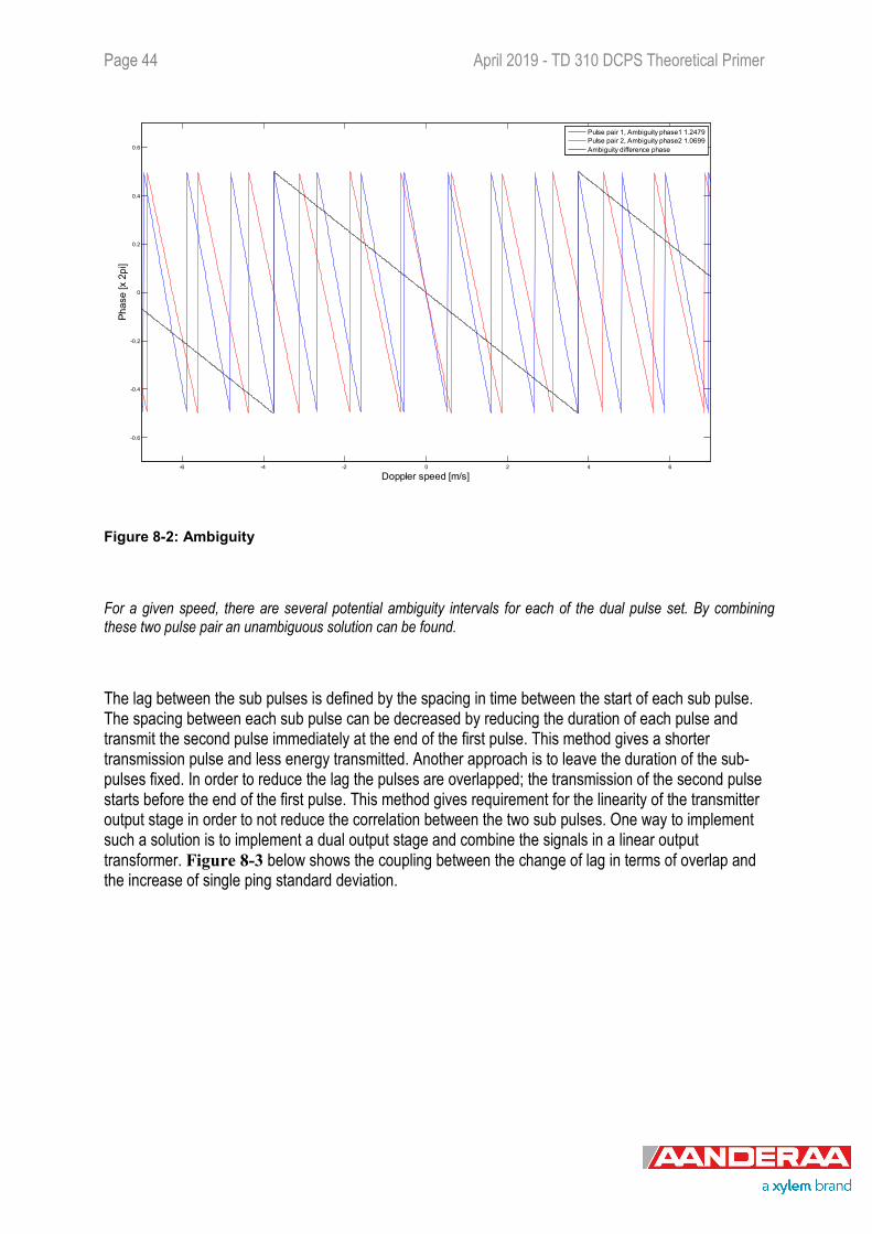
Pulse pair 1, Ambiguity phase1 1.2479Pulse pair 2, Ambiguity phase2 1.0699Ambiguity difference phase
Figure 8-2: Ambiguity
For a given speed, there are several potential ambiguity intervals for each of the dual pulse set. By combining these two pulse pair an unambiguous solution can be found.
The lag between the sub pulses is defined by the spacing in time between the start of each sub pulse. The spacing between each sub pulse can be decreased by reducing the duration of each pulse and transmit the second pulse immediately at the end of the first pulse. This method gives a shorter transmission pulse and less energy transmitted. Another approach is to leave the duration of the sub-pulses fixed. In order to reduce the lag the pulses are overlapped; the transmission of the second pulse starts before the end of the first pulse. This method gives requirement for the linearity of the transmitter output stage in order to not reduce the correlation between the two sub pulses. One way to implement such a solution is to implement a dual output stage and combine the signals in a linear output transformer. Figure 8-3 below shows the coupling between the change of lag in terms of overlap and the increase of single ping standard deviation.
April 2019 - TD 310 DCPS Theoretical Primer Page 45
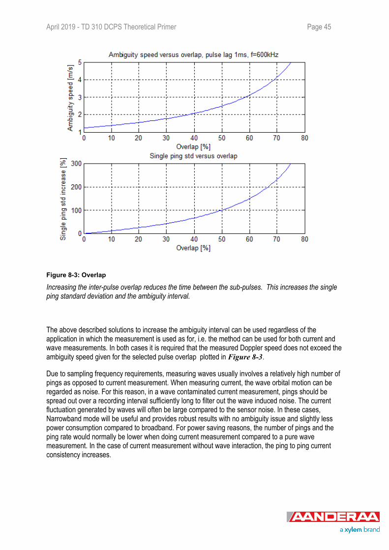
Figure 8-3: Overlap
Increasing the inter-pulse overlap reduces the time between the sub-pulses. This increases the single ping standard deviation and the ambiguity interval.
The above described solutions to increase the ambiguity interval can be used regardless of the application in which the measurement is used as for, i.e. the method can be used for both current and wave measurements. In both cases it is required that the measured Doppler speed does not exceed the ambiguity speed given for the selected pulse overlap plotted in Figure 8-3.
Due to sampling frequency requirements, measuring waves usually involves a relatively high number of pings as opposed to current measurement. When measuring current, the wave orbital motion can be regarded as noise. For this reason, in a wave contaminated current measurement, pings should be spread out over a recording interval sufficiently long to filter out the wave induced noise. The current fluctuation generated by waves will often be large compared to the sensor noise. In these cases, Narrowband mode will be useful and provides robust results with no ambiguity issue and slightly less power consumption compared to broadband. For power saving reasons, the number of pings and the ping rate would normally be lower when doing current measurement compared to a pure wave measurement. In the case of current measurement without wave interaction, the ping to ping current consistency increases.
Page 46 April 2019 - TD 310 DCPS Theoretical Primer
8.3 Adaptive transmission pulse
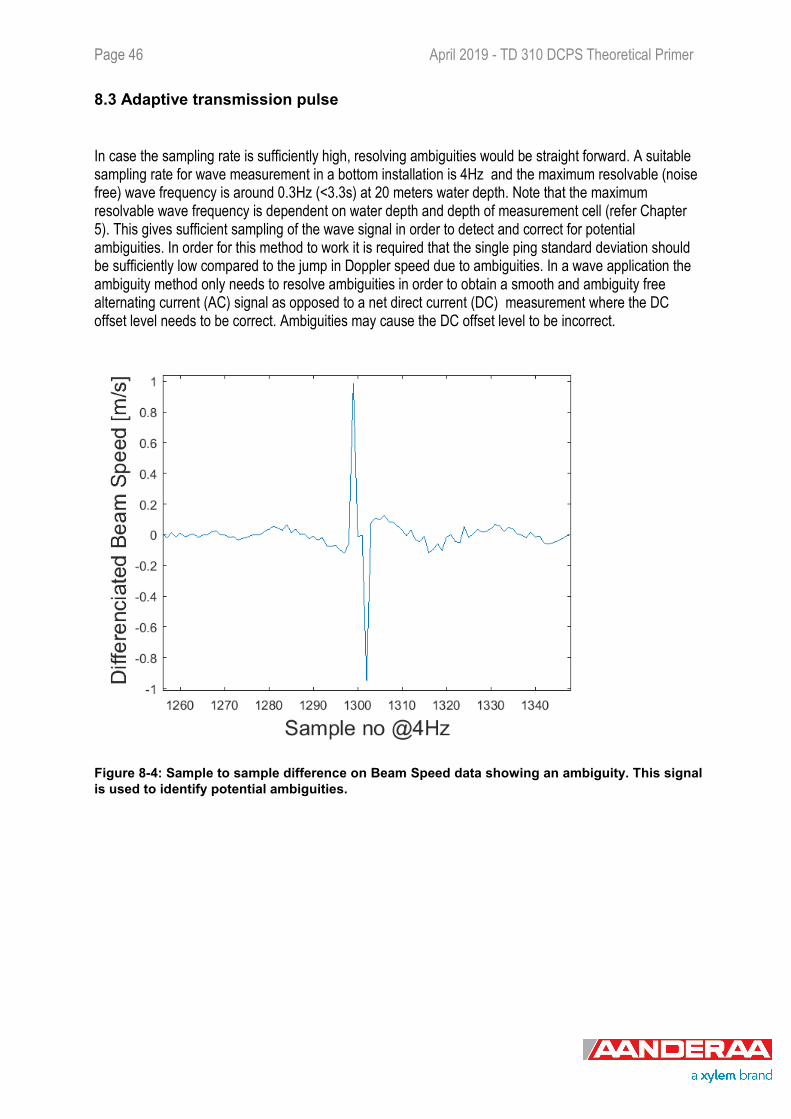
In case the sampling rate is sufficiently high, resolving ambiguities would be straight forward. A suitable sampling rate for wave measurement in a bottom installation is 4Hz and the maximum resolvable (noise free) wave frequency is around 0.3Hz (<3.3s) at 20 meters water depth. Note that the maximum resolvable wave frequency is dependent on water depth and depth of measurement cell (refer Chapter 5). This gives sufficient sampling of the wave signal in order to detect and correct for potential ambiguities. In order for this method to work it is required that the single ping standard deviation should be sufficiently low compared to the jump in Doppler speed due to ambiguities. In a wave application the ambiguity method only needs to resolve ambiguities in order to obtain a smooth and ambiguity free alternating current (AC) signal as opposed to a net direct current (DC) measurement where the DC offset level needs to be correct. Ambiguities may cause the DC offset level to be incorrect.
Figure 8-4: Sample to sample difference on Beam Speed data showing an ambiguity. This signal is used to identify potential ambiguities.
April 2019 - TD 310 DCPS Theoretical Primer Page 47
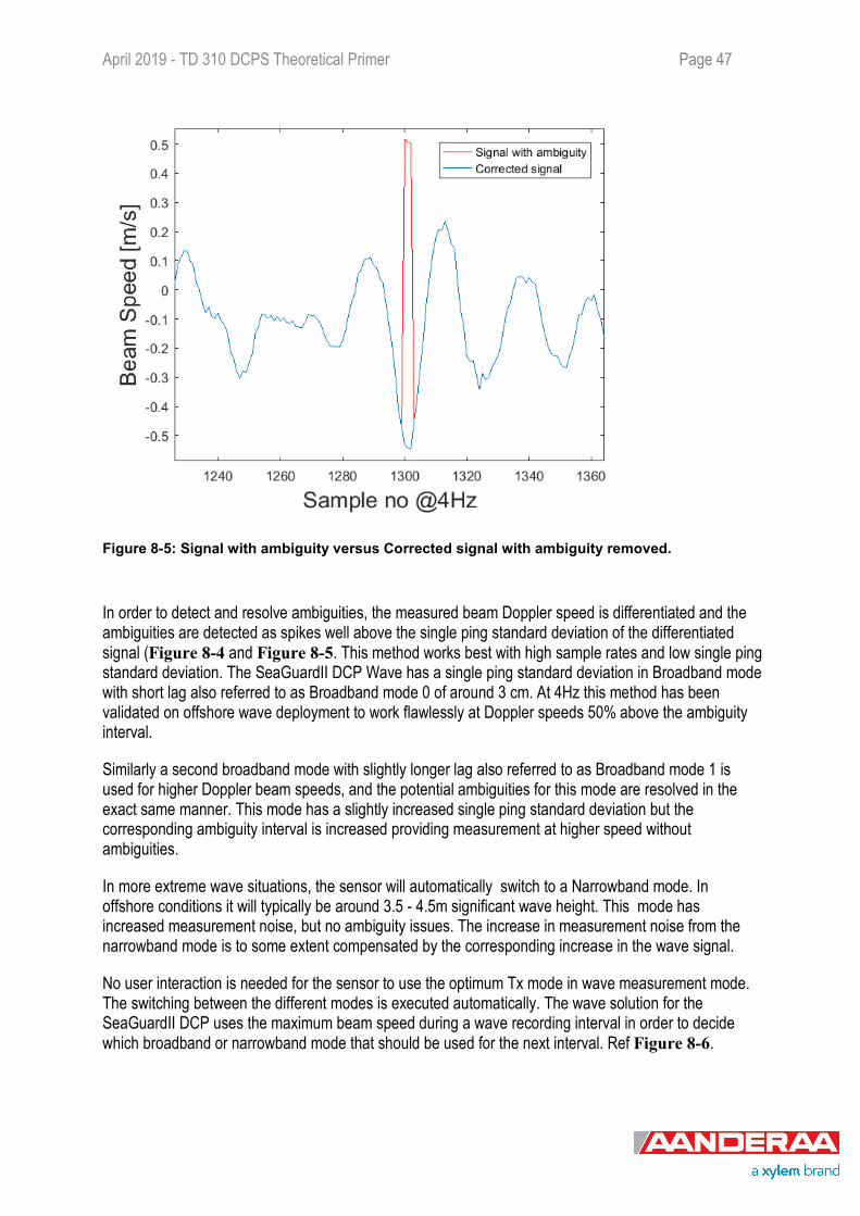
Figure 8-5: Signal with ambiguity versus Corrected signal with ambiguity removed.
In order to detect and resolve ambiguities, the measured beam Doppler speed is differentiated and the ambiguities are detected as spikes well above the single ping standard deviation of the differentiated signal (Figure 8-4 and Figure 8-5. This method works best with high sample rates and low single ping standard deviation. The SeaGuardII DCP Wave has a single ping standard deviation in Broadband mode with short lag also referred to as Broadband mode 0 of around 3 cm. At 4Hz this method has been validated on offshore wave deployment to work flawlessly at Doppler speeds 50% above the ambiguity interval.
Similarly a second broadband mode with slightly longer lag also referred to as Broadband mode 1 is used for higher Doppler beam speeds, and the potential ambiguities for this mode are resolved in the exact same manner. This mode has a slightly increased single ping standard deviation but the corresponding ambiguity interval is increased providing measurement at higher speed without ambiguities.
In more extreme wave situations, the sensor will automatically switch to a Narrowband mode. In offshore conditions it will typically be around 3.5 - 4.5m significant wave height. This mode has increased measurement noise, but no ambiguity issues. The increase in measurement noise from the narrowband mode is to some extent compensated by the corresponding increase in the wave signal.
No user interaction is needed for the sensor to use the optimum Tx mode in wave measurement mode. The switching between the different modes is executed automatically. The wave solution for the SeaGuardII DCP uses the maximum beam speed during a wave recording interval in order to decide which broadband or narrowband mode that should be used for the next interval. Ref Figure 8-6.
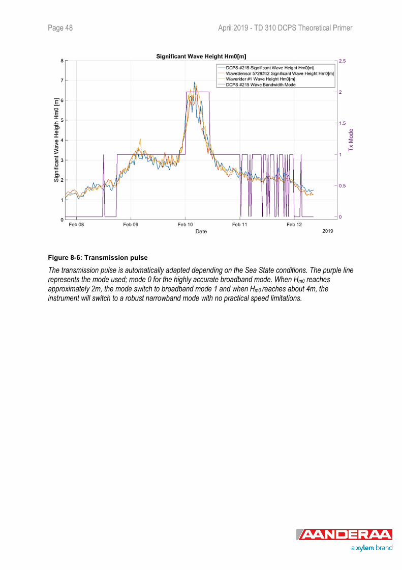
Page 48 April 2019 - TD 310 DCPS Theoretical Primer
Figure 8-6: Transmission pulse
The transmission pulse is automatically adapted depending on the Sea State conditions. The purple line represents the mode used; mode 0 for the highly accurate broadband mode. When Hm0 reaches approximately 2m, the mode switch to broadband mode 1 and when Hm0 reaches about 4m, the instrument will switch to a robust narrowband mode with no practical speed limitations.
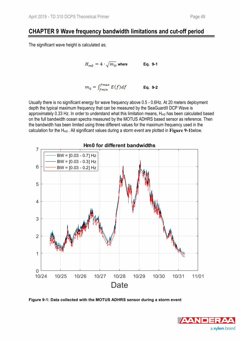
April 2019 - TD 310 DCPS Theoretical Primer Page 49
CHAPTER 9 Wave frequency bandwidth limitations and cut-off period
The significant wave height is calculated as;
, where Eq. 9-1
Eq. 9-2
Usually there is no significant energy for wave frequency above 0.5 - 0.6Hz. At 20 meters deployment depth the typical maximum frequency that can be measured by the SeaGuardII DCP Wave is approximately 0.33 Hz. In order to understand what this limitation means, Hm0 has been calculated based on the full bandwidth ocean spectra measured by the MOTUS ADHRS based sensor as reference. Then the bandwidth has been limited using three different values for the maximum frequency used in the calculation for the Hm0 . All significant values during a storm event are plotted in Figure 9-1below.
Figure 9-1: Data collected with the MOTUS ADHRS sensor during a storm event
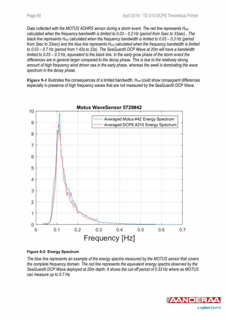
Page 50 April 2019 - TD 310 DCPS Theoretical Primer
Data collected with the MOTUS ADHRS sensor during a storm event. The red line represents Hm0 calculated when the frequency bandwidth is limited to 0.03 – 0.2 Hz (period from 5sec to 33sec) . The black line represents Hm0 calculated when the frequency bandwidth is limited to 0.03 – 0.3 Hz (period from 3sec to 33sec) and the blue line represents Hm0 calculated when the frequency bandwidth is limited to 0.03 – 0.7 Hz (period from 1.43s to 33s). The SeaGuardII DCP Wave at 20m will have a bandwidth limited to 0.03 – 0.3 Hz, equivalent to the black line. In the early grow phase of the storm event the differences are in general larger compared to the decay phase. This is due to the relatively strong amount of high frequency wind driven sea in the early phase, whereas the swell is dominating the wave spectrum in the decay phase.
Figure 9-1 illustrates the consequences of a limited bandwidth. Hm0 could show consequent differences especially in presence of high frequency waves that are not measured by the SeaGuardII DCP Wave.
Figure 9-2: Energy Spectrum
The blue line represents an example of the energy spectra measured by the MOTUS sensor that covers the complete frequency domain. The red line represents the equivalent energy spectra observed by the SeaGuardII DCP Wave deployed at 20m depth: It shows the cut-off period of 0.33 Hz where as MOTUS can measure up to 0.7 Hz.
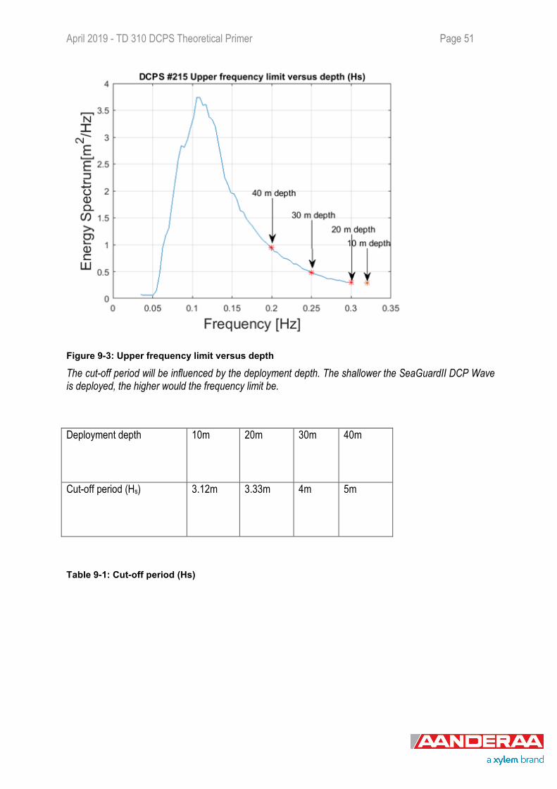
April 2019 - TD 310 DCPS Theoretical Primer Page 51
Figure 9-3: Upper frequency limit versus depth
The cut-off period will be influenced by the deployment depth. The shallower the SeaGuardII DCP Wave is deployed, the higher would the frequency limit be.
Deployment depth 10m 20m 30m 40m
Cut-off period (Hs) 3.12m 3.33m 4m 5m
Table 9-1: Cut-off period (Hs)
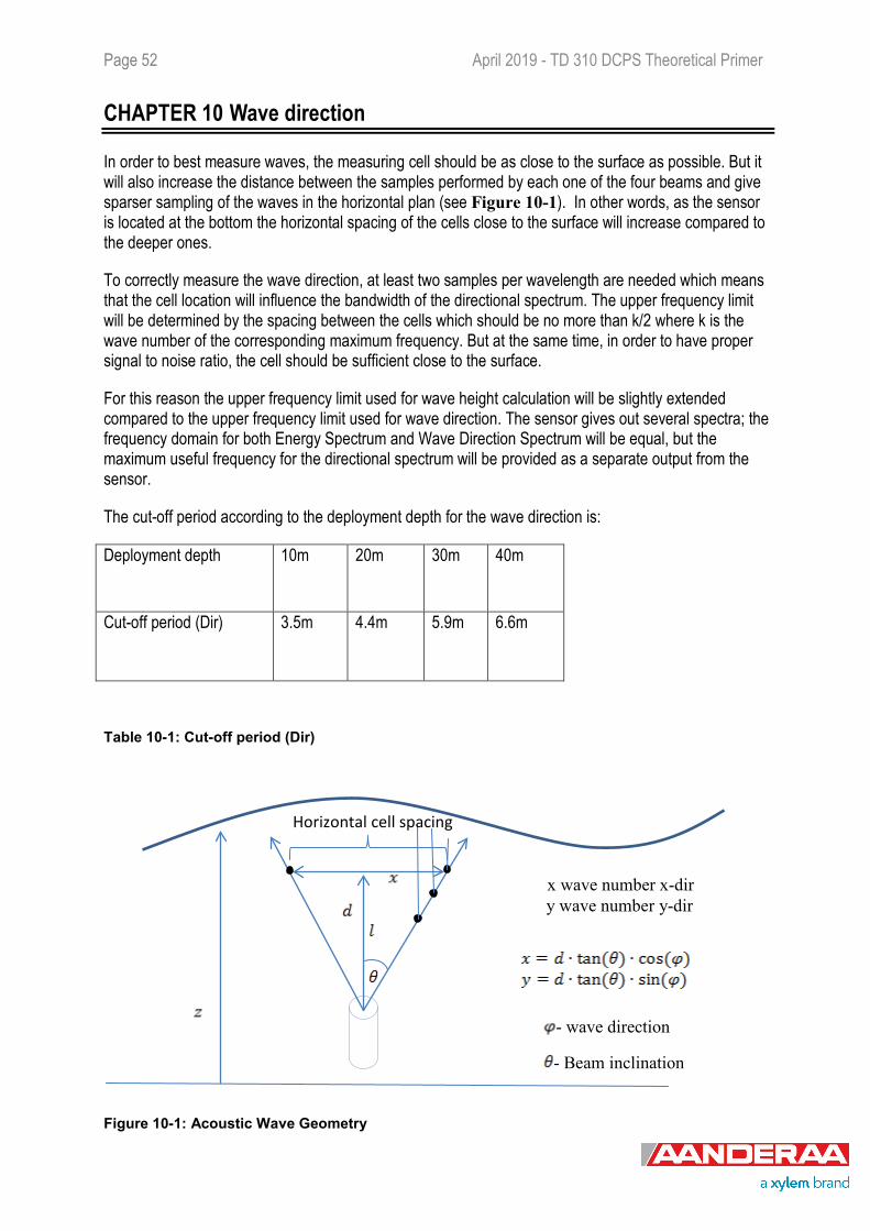
Page 52 April 2019 - TD 310 DCPS Theoretical Primer
CHAPTER 10 Wave direction
In order to best measure waves, the measuring cell should be as close to the surface as possible. But it will also increase the distance between the samples performed by each one of the four beams and give sparser sampling of the waves in the horizontal plan (see Figure 10-1). In other words, as the sensor is located at the bottom the horizontal spacing of the cells close to the surface will increase compared to the deeper ones.
To correctly measure the wave direction, at least two samples per wavelength are needed which means that the cell location will influence the bandwidth of the directional spectrum. The upper frequency limit will be determined by the spacing between the cells which should be no more than k/2 where k is the wave number of the corresponding maximum frequency. But at the same time, in order to have proper signal to noise ratio, the cell should be sufficient close to the surface.
For this reason the upper frequency limit used for wave height calculation will be slightly extended compared to the upper frequency limit used for wave direction. The sensor gives out several spectra; the frequency domain for both Energy Spectrum and Wave Direction Spectrum will be equal, but the maximum useful frequency for the directional spectrum will be provided as a separate output from the sensor.
The cut-off period according to the deployment depth for the wave direction is:
Deployment depth 10m 20m 30m 40m
Cut-off period (Dir) 3.5m 4.4m 5.9m 6.6m
Table 10-1: Cut-off period (Dir)
Figure 10-1: Acoustic Wave Geometry
- wave direction
- Beam inclination
x wave number x-dir y wave number y-dir
Horizontal cell spacing
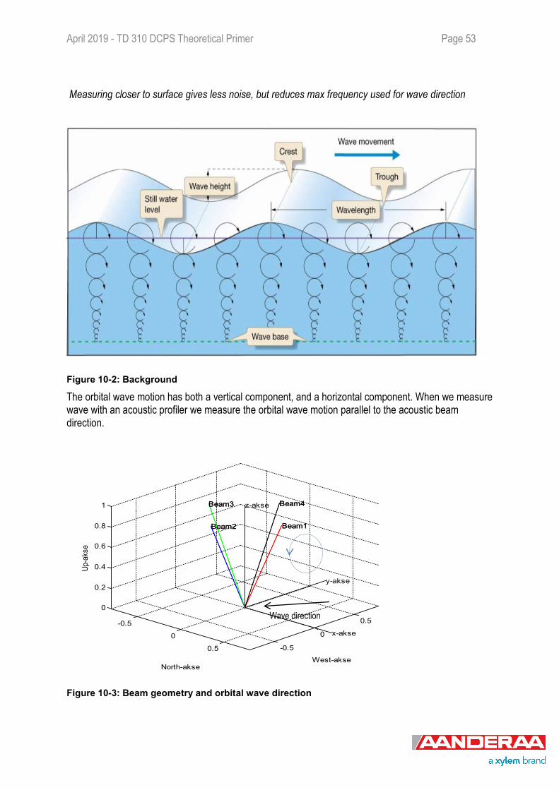
April 2019 - TD 310 DCPS Theoretical Primer Page 53
Measuring closer to surface gives less noise, but reduces max frequency used for wave direction
Figure 10-2: Background
The orbital wave motion has both a vertical component, and a horizontal component. When we measure wave with an acoustic profiler we measure the orbital wave motion parallel to the acoustic beam direction.
Figure 10-3: Beam geometry and orbital wave direction
-0.5
0
0.5 -0.5
0
0.5
0
0.2
0.4
0.6
0.8
1
x-akse
y-akse
West-akse
Beam1 Beam1
Beam4 Beam4 z-akse
Beam2 Beam2
Beam3 Beam3
North-akse
Up-a
kse
Wave direction
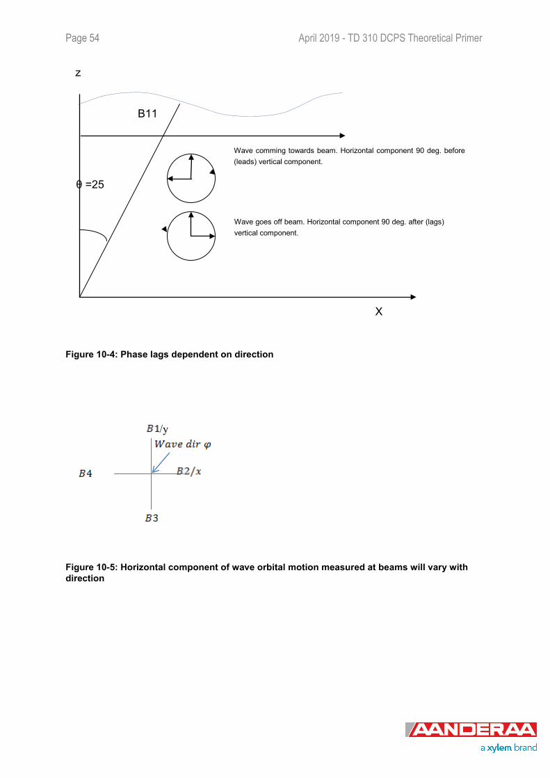
Page 54 April 2019 - TD 310 DCPS Theoretical Primer
Figure 10-4: Phase lags dependent on direction
Figure 10-5: Horizontal component of wave orbital motion measured at beams will vary with direction
θ =25
B11
X
z
Wave comming towards beam. Horizontal component 90 deg. before (leads) vertical component.
Wave goes off beam. Horizontal component 90 deg. after (lags) vertical component.
/y

April 2019 - TD 310 DCPS Theoretical Primer Page 55
All orbital wave components [x,y,z] at B1 and the pointing vector of beam 1 PB1[x,y,z].
Eq. 10-1
Eq. 10-2
Eq. 10-3
The beam speed measured due to the orbital beam speed can be found by calculating the inner product between the Beam pointing vector and the orbital beam speed components at the cell position of the beam of interest.
Eq. 10-4
Let and Eq. 10-5
then we can write the Eq. 10-6
Eq. 10-7
Similarly the beam speeds measured at each beam can be expressed as given in the equations below. These equations give the forward relationship between wave heights:
Eq. 10-8
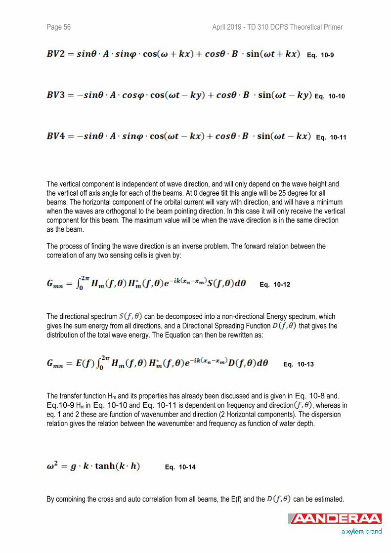
Page 56 April 2019 - TD 310 DCPS Theoretical Primer
Eq. 10-9
Eq. 10-10
Eq. 10-11
The vertical component is independent of wave direction, and will only depend on the wave height and the vertical off axis angle for each of the beams. At 0 degree tilt this angle will be 25 degree for all beams. The horizontal component of the orbital current will vary with direction, and will have a minimum when the waves are orthogonal to the beam pointing direction. In this case it will only receive the vertical component for this beam. The maximum value will be when the wave direction is in the same direction as the beam.
The process of finding the wave direction is an inverse problem. The forward relation between the correlation of any two sensing cells is given by:
Eq. 10-12
The directional spectrum can be decomposed into a non-directional Energy spectrum, which gives the sum energy from all directions, and a Directional Spreading Function that gives the distribution of the total wave energy. The Equation can then be rewritten as:
Eq. 10-13
The transfer function Hm and its properties has already been discussed and is given in Eq. 10-8 and. Eq.10-9 Hm in Eq. 10-10 and Eq. 10-11 is dependent on frequency and direction , whereas in eq. 1 and 2 these are function of wavenumber and direction (2 Horizontal components). The dispersion relation gives the relation between the wavenumber and frequency as function of water depth.
Eq. 10-14
By combining the cross and auto correlation from all beams, the E(f) and the can be estimated.
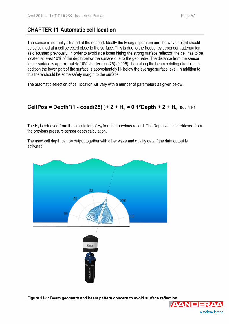
April 2019 - TD 310 DCPS Theoretical Primer Page 57
CHAPTER 11 Automatic cell location
The sensor is normally situated at the seabed. Ideally the Energy spectrum and the wave height should be calculated at a cell selected close to the surface. This is due to the frequency dependent attenuation as discussed previously. In order to avoid side lobes hitting the strong surface reflector, the cell has to be located at least 10% of the depth below the surface due to the geometry. The distance from the sensor to the surface is approximately 10% shorter (cos(25)=0.906) than along the beam pointing direction. In addition the lower part of the surface is approximately Hs below the average surface level. In addition to this there should be some safety margin to the surface.
The automatic selection of cell location will vary with a number of parameters as given below.
CellPos = Depth*(1 - cosd(25) )+ 2 + Hs ≈ 0.1*Depth + 2 + Hs Eq. 11-1
The Hs is retrieved from the calculation of Hs from the previous record. The Depth value is retrieved from the previous pressure sensor depth calculation.
The used cell depth can be output together with other wave and quality data if the data output is activated.
Figure 11-1: Beam geometry and beam pattern concern to avoid surface reflection.

Page 58 April 2019 - TD 310 DCPS Theoretical Primer
CHAPTER 12 Quality parameters
As described in earlier chapters, the transfer function is strongly dependent of the depth position of the measuring cell and the water depth. When this information is correct, the calculated wave height should be equal independent of the selected depth cell. This assumes that the bandwidth used for calculation of the significant wave height is equal for the different cells, and that the upper frequency used in the lower cell is sufficient low such that noise do not contribute to the significant wave height for the lower cell.
The AWS sensor utilizes this feature as a quality parameter. It is possible to calculate the wave height for three independent depth cells. By comparing the data from these three cells, information related to the quality of the significant wave height will be revealed.
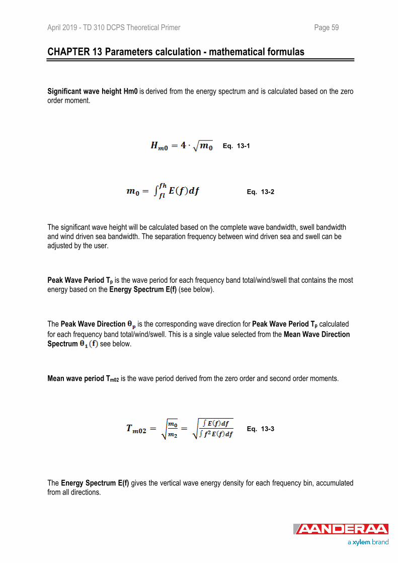
April 2019 - TD 310 DCPS Theoretical Primer Page 59
CHAPTER 13 Parameters calculation - mathematical formulas
Significant wave height Hm0 is derived from the energy spectrum and is calculated based on the zero order moment.
Eq. 13-1
Eq. 13-2
The significant wave height will be calculated based on the complete wave bandwidth, swell bandwidth and wind driven sea bandwidth. The separation frequency between wind driven sea and swell can be adjusted by the user.
Peak Wave Period Tp is the wave period for each frequency band total/wind/swell that contains the most energy based on the Energy Spectrum E(f) (see below).
The Peak Wave Direction is the corresponding wave direction for Peak Wave Period Tp calculated for each frequency band total/wind/swell. This is a single value selected from the Mean Wave Direction Spectrum see below.
Mean wave period Tm02 is the wave period derived from the zero order and second order moments.
Eq. 13-3
The Energy Spectrum E(f) gives the vertical wave energy density for each frequency bin, accumulated from all directions.
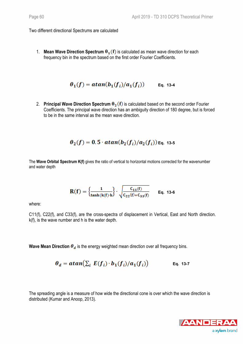
Page 60 April 2019 - TD 310 DCPS Theoretical Primer
Two different directional Spectrums are calculated
1. Mean Wave Direction Spectrum is calculated as mean wave direction for each frequency bin in the spectrum based on the first order Fourier Coefficients.
Eq. 13-4
2. Principal Wave Direction Spectrum is calculated based on the second order Fourier Coefficients. The principal wave direction has an ambiguity direction of 180 degree, but is forced to be in the same interval as the mean wave direction.
Eq. 13-5
The Wave Orbital Spectrum K(f) gives the ratio of vertical to horizontal motions corrected for the wavenumber and water depth
Eq. 13-6
where:
C11(f), C22(f), and C33(f), are the cross-spectra of displacement in Vertical, East and North direction. k(f), is the wave number and h is the water depth.
Wave Mean Direction is the energy weighted mean direction over all frequency bins.
Eq. 13-7
The spreading angle is a measure of how wide the directional cone is over which the wave direction is distributed (Kumar and Anoop, 2013).
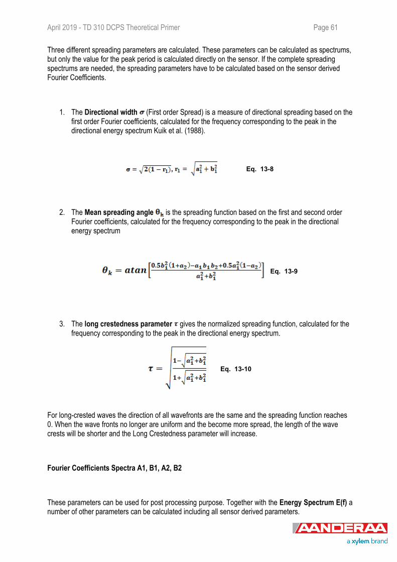
April 2019 - TD 310 DCPS Theoretical Primer Page 61
Three different spreading parameters are calculated. These parameters can be calculated as spectrums, but only the value for the peak period is calculated directly on the sensor. If the complete spreading spectrums are needed, the spreading parameters have to be calculated based on the sensor derived Fourier Coefficients.
1. The Directional width (First order Spread) is a measure of directional spreading based on the first order Fourier coefficients, calculated for the frequency corresponding to the peak in the directional energy spectrum Kuik et al. (1988).
, Eq. 13-8
2. The Mean spreading angle is the spreading function based on the first and second order Fourier coefficients, calculated for the frequency corresponding to the peak in the directional energy spectrum
Eq. 13-9
3. The long crestedness parameter gives the normalized spreading function, calculated for the frequency corresponding to the peak in the directional energy spectrum.
Eq. 13-10
For long-crested waves the direction of all wavefronts are the same and the spreading function reaches 0. When the wave fronts no longer are uniform and the become more spread, the length of the wave crests will be shorter and the Long Crestedness parameter will increase.
Fourier Coefficients Spectra A1, B1, A2, B2
These parameters can be used for post processing purpose. Together with the Energy Spectrum E(f) a number of other parameters can be calculated including all sensor derived parameters.
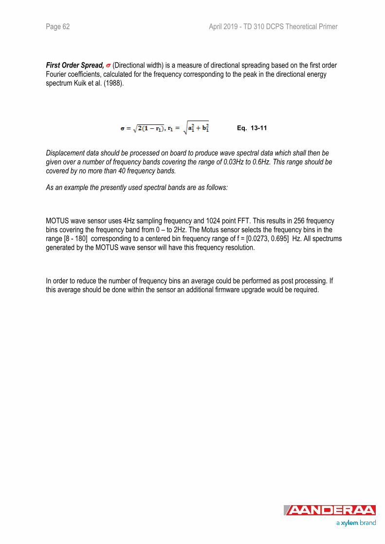
Page 62 April 2019 - TD 310 DCPS Theoretical Primer
First Order Spread, (Directional width) is a measure of directional spreading based on the first order Fourier coefficients, calculated for the frequency corresponding to the peak in the directional energy spectrum Kuik et al. (1988).
, Eq. 13-11
Displacement data should be processed on board to produce wave spectral data which shall then be given over a number of frequency bands covering the range of 0.03Hz to 0.6Hz. This range should be covered by no more than 40 frequency bands.
As an example the presently used spectral bands are as follows:
MOTUS wave sensor uses 4Hz sampling frequency and 1024 point FFT. This results in 256 frequency bins covering the frequency band from 0 – to 2Hz. The Motus sensor selects the frequency bins in the range [8 - 180] corresponding to a centered bin frequency range of f = [0.0273, 0.695] Hz. All spectrums generated by the MOTUS wave sensor will have this frequency resolution.
In order to reduce the number of frequency bins an average could be performed as post processing. If this average should be done within the sensor an additional firmware upgrade would be required.
April 2019 - TD 310 DCPS Theoretical Primer Page 63
CHAPTER 14 References
B. H. Brumley, R. G. Cabrera, K. L. Denies, and E. A. Terray, “Performance of a broad-band acoustic Doppler current profiler,” IEEE J. Oceanic Eng., ol. 16, pp.402-407, 1991.
P. Wanis, B. Brumley, J. Gast, and D. Symonds, “Sources of measurement variance in broadband acoustic Doppler current profilers,” in Proc. MTS/IEEE OCEANS Conf., Seattle, WA, USA, Sep. 2010, DOI: 10.1109/OCEANS.2010.5664327. Ocean. Eng., vol. 16, no. 4, pp. 402-407, Oct. 1991.
Benoit, M Frigaard, P., and Schäffer, H.A. (1997), Analysing multidirectional wave spectra: A tentative classification of available methods, in IAHR Seminar on Multidirectional Waves and their Interaction with Structurs, pp. 131-158, San Francisco, US.
C. Chi, H. Vishnu, and K. T Beng, “Improving broadband acoustic Doppler current profiler with orthogonal coprime pulse pairs and robust chinese reminder theorem.
Francois, R.E., Garrison, G.R., 1982. Sound absorption based on ocean measurements. Part II: Boric acid contribution and equation for total absorption. J. Acoust. Soc. Am. 72 1879-1890
Simpson, M.R., 2001, Discharge measurements using a broadband acoustic Doppler current profiler. United States Geological Survey, Open-file-report 01-1
Urick, R.J., 1983, Principles of underwater sound. (3rd edition): McGraw-Hill, San Francisco, USA
Kinsler & Frey, Fundamentals of Acoustics. (3rd edition): John Wiley & Sons
François Le Chevalier, Principles of Radar and Sonar Signal Processing, Artech House Publishers
Almroth-Rosell E., A. Tengberg, S. Andersson, A. Apler and P.O.J. Hall (2012). Effects of simulated natural and massive resuspension on benthic oxygen, nutrient and dissolved inorganic carbon fluxes in Loch Creran, Scotland. Journal of Sea Research, 72, 38-48.
Atamanchuk D., M. Kononets, P.J. Thomas, J. Hovdenes, A. Tengberg and P.O.J. Hall (2015) Continuous long-term observations of the carbonate system dynamics in the water column of a temperate fjord.
Journal of Marine Systems, 148, 272–284.
Francis O.P. and D. E. Atkinson (2012) Synoptic forcing of wave states in the southeast Chukchi Sea, Alaska, at nearshore locations . Natural Hazards, 62: 1273–1300.
Francis O.P. and D. E. Atkinson (2012) Synoptic forcing of wave states in the southeast Chukchi Sea, Alaska, at an offshore location. Natural Hazards, 62: 1169–1189.
Francis O.P., G.G. Panteleev and D. E. Atkinson(2011) Ocean wave conditions in the Chukchi Sea from satellite and in situ observations. Geophysical Research Letters, 38, L24610, doi:10.1029/2011GL049839.
Page 64 April 2019 - TD 310 DCPS Theoretical Primer
Friedrich J., F. Janssen, D. Aleynik, H.W. Bange, N. Boltacheva, M.N. Çaǧatay, A.W. Dale, G. Etiope, Z. Erdem, M. Geraga, A. Gilli, M.T. Gomoiu, P.O.J. Hall, D. Hansson, Y. He, M. Holtappels, M. K. Kirf, M. Kononets, S. Konovalov, A. Lichtschlag, D. M. Livingstone, G. Marinaro, S. Mazlumyan, S. Naeher, 17, R.P. North, G. Papatheodorou, O. Pfannkuche, R. Prien, G. Rehder, C.J. Schubert, T. Soltwedel, S. Sommer, H. Stahl, E. V. Stanev, A. Teaca, A. Tengberg, C. Waldmann, B. Wehrli and F. Wenzhöfer (2014). Investigating hypoxia in aquatic environments: diverse approaches to addressing a complex phenomenon. Biogeosciences, 11, 1215–1259.
Oguri K., Y. Furushima, T. Toyofuku, T. Kasaya, M. Wakita, S. Watanabe, K. Fujikura, H. Kitazato (2015). Long-term monitoring of bottom environments of the continental slope off Otsuchi Bay, northeastern Japan . Journal of Oceanography, Special Issue Oceanographic Observations After The 2011 Earthquake Off The Pacific Coast Of Tohoku, pp 1-16.
Suursaar U. (2010) Waves, currents and sea level variations along the Letipea – Sillamae coastal section of the southern Gulf of Finland. Oceanologia, 52 (3), 391–416.
Suursaar U. and R. Aps (2007) Spatio-temporal variations in hydro-physical and -chemical parameters during a major upwelling event off the southern coast of the Gulf of Finland in summer 2006. Oceanologia, 49 (2), 209–228.
Suursaar U, J. Jaagus, A. Kontc, R. Rivis, H. Tonisson (2008) Field observations on hydrodynamic and coastal geomorphic processes off Harilaid Peninsula (Baltic Sea) in winter and spring 2006–2007. Estuarine, Coastal and Shelf Science, 80, 31–41.
Suursaar U., T. Kullas and R. Aps (2012) Currents and waves in the northern Gulf of Riga: measurement and long-term hindcast. Oceanologia, 54 (3), 421–447.
Tengberg A., E. Almroth and P.O.J. Hall (2003). Resuspension and its effect on organic carbon recycling and nutrient exchange in coastal sediments: In-situ measurements using new experimental technology. Journal of Experimental Marine Biology and Ecology, 285-286: 119-142.
Wesslander K., P. Hall, S. Hjalmarsson, D. Lefevre, A. Omstedt, A. Rutgersson, E. Sahlée and A. Tengberg (2011) Observed carbon dioxide and oxygen dynamics in a Baltic Sea coastal region. Journal of Marine Systems, 86: 1–9.
Harold V. Thurman, Alan P. Trujillo (2001) Essentials of Oceanography, Seventh edition

April 2019 - TD 310 DCPS Theoretical Primer Page 65
Aanderaa Data Instruments AS P.O.Box 103 Midtun, Sanddalsringen 5b, N-5843 Bergen, Norway Tel: +47 55 60 48 00 Fax: +47 55 60 48 01 email: [email protected] - www.aanderaa.com
Aanderaa Data Instruments AS is a trademark of Xylem Inc. or one of its subsidiaries. © 2019 Xylem, Inc. April 2019