M

Ja

b

a

ARRAA

KDDFC

1

ppfmbtfs(st[bph

u

Pf

0d

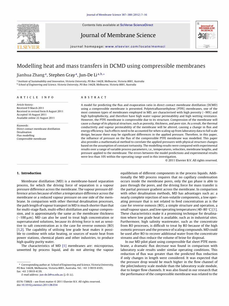
Journal of Membrane Science 387– 388 (2012) 7– 16

Contents lists available at SciVerse ScienceDirect

Journal of Membrane Science

jo u rn al hom epa ge: www.elsev ier .com/ locate /memsci

odelling heat and mass transfers in DCMD using compressible membranes

ianhua Zhanga, Stephen Graya, Jun-De Lia,b,∗

Institute of Sustainability and Innovation, Victoria University, PO Box 14428, Melbourne, Victoria 8001, AustraliaSchool of Engineering and Science, Victoria University, PO Box 14428, Melbourne, Victoria 8001, Australia

r t i c l e i n f o

rticle history:eceived 9 March 2011eceived in revised form 8 August 2011ccepted 10 August 2011vailable online 22 August 2011

eywords:irect contact membrane distillationesalinationlux modelling

a b s t r a c t

A model for predicting the flux and evaporation ratio in direct contact membrane distillation (DCMD)using a compressible membrane is presented. Polytetrafluoroethylene (PTFE) membranes, one of themost common types of membranes employed in MD, are characterised with high porosity (∼90%) andhigh hydrophobicity, and therefore have high water vapour permeability and high wetting resistance.However, the PTFE membrane is compressible due to its structure. Compression of the membrane willcause a change of its physical structure, such as porosity, thickness, and pore size. As a result, the thermalconductivity and vapour permeability of the membrane will be altered, causing a change in flux andenergy efficiency. Such effects need to be accounted for when scaling up from laboratory data to full scaledesign, because there may be significant differences in the applied pressure. Therefore, in this paper,

ompressible membrane the influence of pressure on the flux of the compressible PTFE membrane was modelled. This paperalso provides a mathematical method to correlate the applied pressures with physical structure changesbased on the assumption of constant tortuosity. The modelling results were compared with experimentalresults over a range of variable process parameters, i.e., temperatures, velocities, membrane lengths, andpressure applied to the membrane. The errors between the model predictions and experimental results

n the

were less than 10% withi

. Introduction

Membrane distillation (MD) is a membrane-based separationrocess, for which the driving force of separation is a vapourressure difference across the membrane. The vapour pressure dif-erence arises because of either a temperature difference across the

embrane or a reduced vapour pressure on one side of the mem-rane. In comparison with other thermal desalination processes,he path length of vapour transport in MD is much shorter than thator multi-stage flash, multi-effect distillation and vapour compres-ion, and is approximately the same as the membrane thickness∼100 �m). MD can also be used to treat high concentration orupersaturated solutions, because its driving force is not as sensi-ive to salt concentration as is the case for reverse osmosis (RO)1,2]. The capability of utilising low grade heat makes it possi-le to combine with solar heating, or sources of waste heat fromower stations, chemical plants and other industries, to produce

igh quality purity water.

The characteristics of MD [1] membranes are: microporous,nwetted by process liquid, and do not altering the vapour

∗ Corresponding author at: School of Engineering and Science, Victoria University,O Box 14428, Melbourne, Victoria 8001, Australia. Tel.: +61 3 9919 4105;ax: +61 3 9919 4139.

E-mail address: jun-de.li@vu.edu.au (J.-D. Li).

376-7388/$ – see front matter © 2011 Elsevier B.V. All rights reserved.oi:10.1016/j.memsci.2011.08.034

operating range used in this investigation.© 2011 Elsevier B.V. All rights reserved.

equilibrium of different components in the process liquids. Addi-tionally the MD process requires that no capillary condensationoccurs inside the membrane pores, only the gas phase is able topass through the pores, and the driving force for mass transfer isthe partial pressure gradient across the membrane. In comparisonwith other desalination methods, MD has advantages such as: anearly complete rejection of non-volatile components, a low oper-ating pressure that is not related to feed concentration as is thecase for reverse osmosis (RO), a simple structure and operation, asmall vapour space, and low operating temperatures (40–80 ◦C) [1].These characteristics make it a promising technique for desalina-tion where low grade heat is available, such as in industrial sites.Furthermore, high salinity wastewater, such as the concentratefrom RO processes, is difficult to treat by RO because of the highosmotic pressure and the presence of scaling compounds. MD couldbe used after RO to recover additional water from the concentratestreams and thus reduce the volume of brine for disposal.

In our MD pilot plant using compressible flat sheet PTFE mem-brane, a dramatic flux decrease was found in comparison withlaboratory scale results under similar operating conditions. Thisreduction of flux was greater than the predicted flux reductionif only changes in length were considered. It was expected that

the pressure drop would be much higher in the flow channel ofthe pilot/industry scale module than the laboratory scale module,due to longer flow channels. It was also found in our research thatthe performance of the compressible membrane was related to the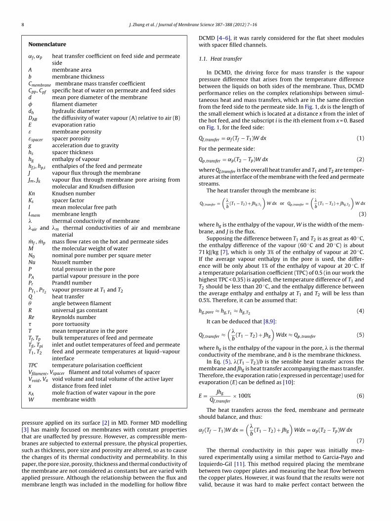

8 J. Zhang et al. / Journal of Membrane

Nomenclature

˛f, ˛p heat transfer coefficient on feed side and permeateside

A membrane areab membrane thicknessCmembrane membrane mass transfer coefficientCpp, Cpf specific heat of water on permeate and feed sidesd mean pore diameter of the membrane� filament diameterdh hydraulic diameterDAB the diffusivity of water vapour (A) relative to air (B)E evaporation ratioε membrane porosityεspacer spacer porosityg acceleration due to gravityhs spacer thicknesshg enthalpy of vapourhf,i, hp,i enthalpies of the feed and permeateJ vapour flux through the membraneJm, Jk vapour flux through membrane pore arising from

molecular and Knudsen diffusionKn Knudsen numberKs spacer factorl mean molecular free pathLmem membrane length� thermal conductivity of membrane�air and �m thermal conductivities of air and membrane

materialmf , mp mass flow rates on the hot and permeate sidesM the molecular weight of waterN0 nominal pore number per square meterNu Nusselt numberP total pressure in the porePA partial vapour pressure in the porePr Prandtl numberPT1 , PT2 vapour pressure at T1 and T2Q heat transfer� angle between filamentR universal gas constantRe Reynolds number� pore tortuosityT mean temperature in the poreTf, Tp bulk temperatures of feed and permeateTfi, Tpi inlet and outlet temperatures of feed and permeateT1, T2 feed and permeate temperatures at liquid–vapour

interfaceTPC temperature polarisation coefficientVfilament, Vspacer filament and total volumes of spacerVvoid, Va void volume and total volume of the active layerx distance from feed inletx mole fraction of water vapour in the pore

p[tbstptam

AW membrane width

ressure applied on its surface [2] in MD. Former MD modelling3] has mainly focused on membranes with constant propertieshat are unaffected by pressure. However, as compressible mem-ranes are subjected to external pressure, the physical properties,uch as thickness, pore size and porosity are altered, so as to causehe changes of its thermal conductivity and permeability. In this

aper, the pore size, porosity, thickness and thermal conductivity ofhe membrane are not considered as constants but are varied withpplied pressure. Although the relationship between the flux andembrane length was included in the modelling for hollow fibre

Science 387– 388 (2012) 7– 16

DCMD [4–6], it was rarely considered for the flat sheet moduleswith spacer filled channels.

1.1. Heat transfer

In DCMD, the driving force for mass transfer is the vapourpressure difference that arises from the temperature differencebetween the liquids on both sides of the membrane. Thus, DCMDperformance relies on the complex relationships between simul-taneous heat and mass transfers, which are in the same directionfrom the feed side to the permeate side. In Fig. 1, dx is the length ofthe small element which is located at a distance x from the inlet ofthe hot feed, and the subscript i is the ith element from x = 0. Basedon Fig. 1, for the feed side:

Qf,transfer = ˛f (Tf − T1)W dx (1)

For the permeate side:

Qp,transfer = ˛p(T2 − Tp)W dx (2)

where Qf,transfer is the overall heat transfer and T1 and T2 are temper-atures at the interface of the membrane with the feed and permeatestreams.

The heat transfer through the membrane is:

Qf,transfer =(

�

b(T1 − T2) + Jhg,T1

)W dx or Qp,transfer =

(�

b(T1 − T2) + Jhg,T2

)W dx

(3)

where hg is the enthalpy of the vapour, W is the width of the mem-brane, and J is the flux.

Supposing the difference between T1 and T2 is as great as 40 ◦C,the enthalpy difference of the vapour (60 ◦C and 20 ◦C) is about71 kJ/kg [7], which is only 3% of the enthalpy of vapour at 20 ◦C.If the average vapour enthalpy in the pore is used, the differ-ence will be only about 1% of the enthalpy of vapour at 20 ◦C. Ifa temperature polarisation coefficient (TPC) of 0.5 (in our work thehighest TPC < 0.35) is applied, the temperature difference of T1 andT2 should be less than 20 ◦C, and the enthalpy difference betweenthe average enthalpy and enthalpy at T1 and T2 will be less than0.5%. Therefore, it can be assumed that:

hg,pore ≈ hg,T1 ≈ hg,T2 (4)

It can be deduced that [8,9]:

Qf,transfer ≈(

�

b(T1 − T2) + Jhg

)Wdx ≈ Qp,transfer (5)

where hg is the enthalpy of the vapour in the pore, � is the thermalconductivity of the membrane, and b is the membrane thickness.

In Eq. (5), �(T1 − T2)/b is the sensible heat transfer across themembrane and Jhg is heat transfer accompanying the mass transfer.Therefore, the evaporation ratio (expressed in percentage) used forevaporation (E) can be defined as [10]:

E = Jhg

Qf,transfer× 100% (6)

The heat transfers across the feed, membrane and permeateshould balance, and thus:

˛f (Tf − T1)W dx =(

�

b(T1 − T2) + Jhg

)Wdx = ˛p(T2 − Tp)W dx

(7)

The thermal conductivity in this paper was initially mea-sured experimentally using a similar method to Garcia-Payo and

Izquierdo-Gil [11]. This method required placing the membranebetween two copper plates and measuring the heat flow betweenthe copper plates. However, it was found that the results were notvalid, because it was hard to make perfect contact between the

J. Zhang et al. / Journal of Membrane Science 387– 388 (2012) 7– 16 9

nsfer

citc

bmemcbtt1sswlt

�

wam

e

T

1

toP

K

iim

os

o0E

Abe calculated as:

xA = PA

P(13)

Table 1Mass transfer mechanism in membrane pore.

Fig. 1. Heat and mass tra

ompressible membrane and the copper discs without compress-ng the membrane. Therefore, it is difficult to judge if the measuredhermal conductivity was overestimated (if the membrane wasompressed) or underestimated (if contact was not good).

For the calculation of thermal conductivity of porous mem-ranes, previous studies [11,12] have determined mathematicodels to fit experimental results. In those papers, a method to

nsure good contact between the membrane and copper discs wasentioned, but there was no discussion of whether this contact

aused deformation of the membrane, especially for the PTFE mem-ranes studied. Therefore, these models may not be applicable forhe PTFE compressible membranes used in this study. Furthermore,he tortuosity factor of the employed PTFE membrane was about.1 [2]. This indicates that the pore channels were approximatelytraight and perpendicular to the membrane surface, so it can bepeculated that the pores and the solid walls between the poresere aligned almost parallel. Therefore, a conservative and popu-

ar parallel model [8,9,13] in MD modelling was used to calculatehermal conductivity of the active layer:

active = �airε + �solid(1 − ε) (8)

here �active, �air and �solid are the thermal conductivities of thective layer, air and the solid material, respectively, and ε is theembrane porosity.The TPC [14] for DCMD is normally used to evaluate the process

fficiency of DCMD and is defined as:

PC = T1 − T2

Tf − Tp(9)

.2. Mass transfer in DCMD

The hydrophobic MD membrane is a porous medium. The massransfer through such medium can be interpreted by three kindsf basic mechanisms: Knudsen diffusion, molecular diffusion andoiseuille flow [15]. The Knudsen number (Kn):

n = l

d(10)

s used to judge the dominating mechanism of the mass transfern the pores. Here, l is the mean free path of the transferred gas

olecules and d is the mean pore diameter of the membrane.Table 1 shows the dominating mass transfer mechanism based

n Kn in a gas mixture with a uniform pressure throughout theystem [16].

As the pore size of the MD membranes is in general in the rangef 0.2–1.0 �m [17] and the mean free path of the water vapour is.11 �m at a feed temperature of 60 ◦C [18], Kn calculated fromq. (10) is in the range of 0.55–0.11. Therefore, Knudsen-molecular

through the membrane.

transition diffusion is the dominating mass transfer mechanismwithin the pores [18,19]. Since the mean pore size of the mem-brane was measured using a gas permeation technique, its usedas the mean pore size for modelling gas diffusion across the mem-brane has the potential to affect the mass transfer modelling results.However, Woods et al. [20] have shown that the effect of pore sizedistribution is small compared to the uncertainties in modellingand experimental reproducibility for DCMD. Therefore the effect ofpore size distribution was ignored in this model.

With this assumption, the overall mass flux across the mem-brane can be expressed as:

1J

= 1Jk

+ 1Jm

= 1

(4/3)d(ε/b�)√

1/(2�RMT)�P

+ 1(1/(1 − xA) · (ε/b�) · (DAB/RT))�P

(11)

where Jm and Jk are the vapour flux through the membrane aris-ing from molecular and Knudsen diffusion, � is the pore tortuosityfactor, R is the universal gas constant, M is the molecular mass ofthe vapour, DAB is the diffusivity of water (A) to air (B), xA is themole fraction of water in the pore and PT1 and PT2 are the vapourpressures at temperature T1 and T2, which can be calculated by theAntoine equation [21].

2. Theory

2.1. Variation of membrane properties with pressure

2.1.1. Mass transfer of compressed membranesIn Eq. (11), the diffusivity (DAB) of water vapour (A) relative to

air (B) can be modelled in membrane distillation as [19,22]:

DAB = 1.895 × 10−5T2.072

P(12)

In this study, as the absolute pressure (100–160 kPa) in the poresis low, the water vapour and air in the pores can be assumed an idealgas mixture. Therefore, the mole fraction of the water vapour x can

Kn < 0.01 0.01 < Kn < 1 Kn > 1

Molecular diffusion Knudsen-molecular diffusiontransition mechanism

Knudsenmechanism

1 brane

c

J

tpbnc

ε

waotm

N

tcmb

d

wdtPptinmdtt

e

J

J

wu

2

idSswd

0 J. Zhang et al. / Journal of Mem

So the total vapour flux across the membrane shown in Eq. (11)an be derived as:

= 7.81 × εd

b�

MT1.072

5.685√

2�RMT + 4dR(P − PA)(PT1 − PT2 ) (14)

As the membrane is compressed, it has been shown [8] that thehickness of the active layer is reduced. As a result, the pore size,orosity and tortuosity are expected to change. As the active mem-rane layer considered in this work was a uniform membrane (i.e.on-asymmetric) with a coarse, porous scrim support, the porosityan be calculated as:

= Vvoid

Va= N0(�d2/4)b�0.5

b= N0

�d2�0.5

4(15)

here N0 is the nominal number of pores per square meter in thective layer, and Vvoid, and Va are the void volume and total volumef the active layer, respectively. In Eq. (15), we have assumed thathe pores are cylindrical. Because porosity and pore size can be

easured by the methods provided in [2], N0 can be estimated by:

0 = 4ε0

�d20�0.5

0

(16)

Here subscript 0 is for memebrane under no compression. Underhe assumption that N0 does not change with pressure, using thehanges in membrane thickness and porosity with pressure deter-ined experimentally, the pore size under different pressures can

e calculated by:

p =√

4εp

N0��0.5p

(17)

here εp, �p and dp are the porosity, tortuosity factor and poreiameter of the membrane at pressure P. In Eq. (17), the change ofortuosity factor (�p) with pressure is unknown for the employedTFE membrane, but was assumed not to change greatly for theressure range considered, i.e. it is assumed �p = �0. This assump-ion was based on a calculated tortuosity factor around 1.1 [2],.e. the pores were almost vertically aligned, and pressure appliedormally will not distort the pores in the direction normal to theembrane greatly. Therefore, the compression of the membrane

oes not affect the ratio of pore length to membrane thickness (tor-uosity) greatly, as the pore length is almost equal to the membranehickness.

The total flux of a membrane under pressure can thus bexpressed as:

= 7.81 × ε√

(4εp)/(N0��0.50 )

b�0

× MT1.072

5.685√

2�RMT + 4√

(4εp)/(N0��0.50 )R(P − PA)

(PT1 − PT2 )

(18)

Eq. (18) can also be simplified to:

p = Cmembrane,p(PT1 − PT2 ) (19)

here Cmembrane,p is the mass transfer coefficient of the membranender pressure.

.1.2. Thermal conductivity of the compressed membrane

As shown in Eq. (8), the thermal conductivity of the membranes related to the porosity. For a compressed membrane, the porosityecreases so the thermal conductivity of the membrane increases.

ince the porosity change with pressure is experimentally mea-urable, the variation of thermal conductivity of the active layerith pressure can be estimated via Eq. (8) [2]. The thermal con-uctivity of the whole membrane was calculated by adding the

Science 387– 388 (2012) 7– 16

thermal conductivities of the scrim layer and the active layer inseries.

2.2. Theoretical analyses of the heat transfer and mass transfer

When developing a model for heat and mass transfer across themembranes, the following assumptions were made:

• no heat loss through the module wall (<1% estimated heat of thefeed),

• the heat of vaporisation and condensation does not change withconcentration, because low concentration feed (1 wt%) was used,and no obvious difference between deionised water and this feedwas found in the previous experiments,

• the tortuosity does not change with pressure,• in balancing the heat transfer, variations in latent heat at different

interface temperatures is ignored, and• there is no temperature gradient across the width of the mem-

brane (i.e. perpendicular to the flow direction).

To analyse the heat transfer between the hot feed and thecold permeate, a small element was considered as shown in theschematic diagram in Fig. 1. Based on Fig. 1, the energy balanceequations for feed and permeate temperatures distributed alongthe membrane can be written as:

mf,ihf,i = mf,i+1hf,i+1 + Qtransfer,i and mp,ihp,i + Qtransfer,i = mp,i+1hp,i+1 (20)

where mf and mp are the mass flow rates of the feed and permeate,and hf,i and hp,i are the enthalpies of the feed and permeate.

Due to the mass transfer across the membrane, the mass flowrates of the feed and permeate are related as:

mf,i = mf,i+1 + JiW dx and mp,i + JiW dx = mp,i+1 (21)

By using the Qf,transfer and Qp,transfer from Eqs. (1) and (2), thetemperature of the feed and permeate at i + 1 can be calculated as:

Tf,i+1 = mf,iCp,f,iTf,i − ˛f (Tf,i − Tf 1,i)W dx

Cp,f,i+1mf,i+1and

Tp,i+1 = mf,iCp,p,iTp,i + ˛p(Tp,i − T1,i)W dx

Cp,p,i+1mp,i+1

(22)

where Cp,f and Cp,p are the specific heats of the feed and permeate.

3. Experiment and simulation

3.1. Membrane characterisation

Membrane materials were provided by Changqi Co. Ltd. andconsisted of a polytetrafluoroethylene (PTFE) active layer and apolypropylene (PP) scrim support layer. The nominal pore size was0.5 �m.

3.1.1. SEM characterisationThe active layer, support layer and the cross section (thickness)

of the membrane were observed by a Philips XL30 FEG ScanningElectron Microscope (SEM). The membrane was fractured followingimmersion in liquid nitrogen to form an intact cross section [10]before it was scanned.

3.1.2. Air permeability measurementThe pore size of the membrane and d0ε0/b0�0 were estimated

by the gas permeability method [19] using compressed nitrogen

and by varying the pressure in the range of 5–80 kPa. The pres-sure difference across the membrane was set at 1.00 ± 0.01 kPa.A digital manometer (645, TPI) was used to measure the pres-sure and the pressure difference. A stopwatch was used to record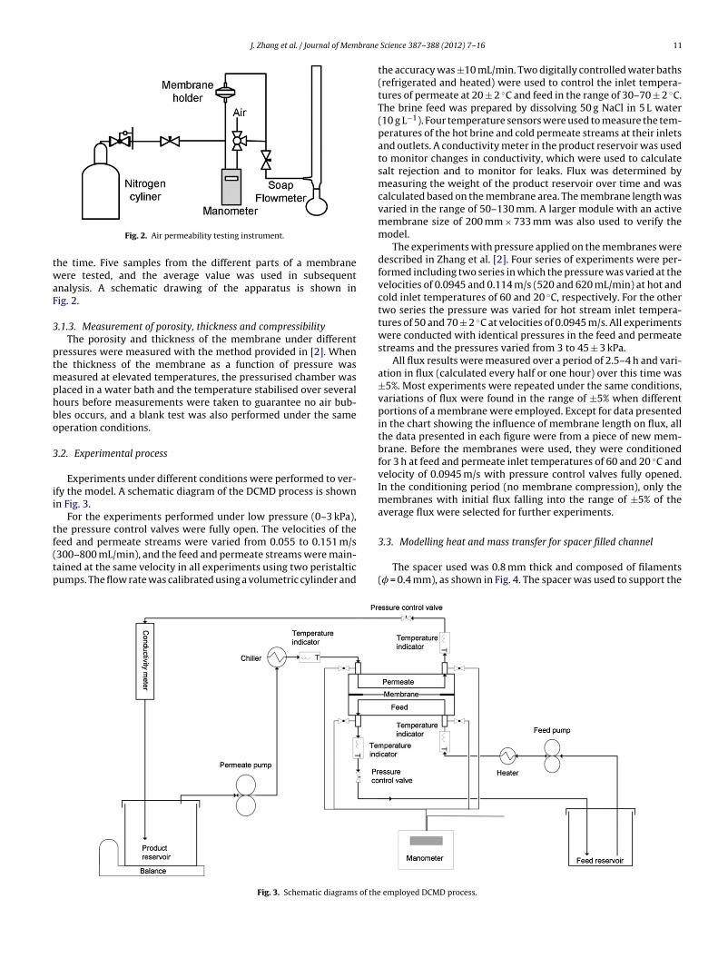

J. Zhang et al. / Journal of Membrane

twaF

3

ptmphbo

3

ii

tf(tp

Fig. 2. Air permeability testing instrument.

he time. Five samples from the different parts of a membraneere tested, and the average value was used in subsequent

nalysis. A schematic drawing of the apparatus is shown inig. 2.

.1.3. Measurement of porosity, thickness and compressibilityThe porosity and thickness of the membrane under different

ressures were measured with the method provided in [2]. Whenhe thickness of the membrane as a function of pressure was

easured at elevated temperatures, the pressurised chamber waslaced in a water bath and the temperature stabilised over severalours before measurements were taken to guarantee no air bub-les occurs, and a blank test was also performed under the sameperation conditions.

.2. Experimental process

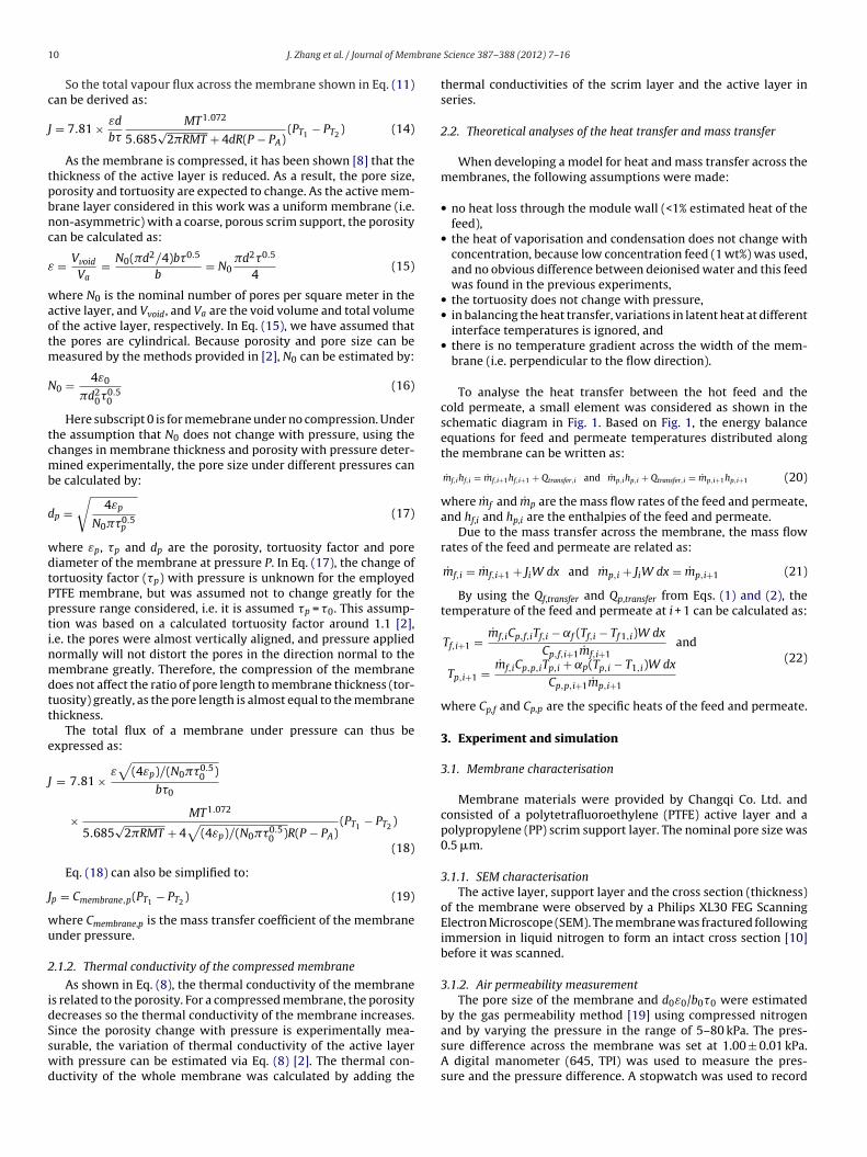
Experiments under different conditions were performed to ver-fy the model. A schematic diagram of the DCMD process is shownn Fig. 3.

For the experiments performed under low pressure (0–3 kPa),he pressure control valves were fully open. The velocities of the

eed and permeate streams were varied from 0.055 to 0.151 m/s300–800 mL/min), and the feed and permeate streams were main-ained at the same velocity in all experiments using two peristalticumps. The flow rate was calibrated using a volumetric cylinder and

Fig. 3. Schematic diagrams of the

Science 387– 388 (2012) 7– 16 11

the accuracy was ±10 mL/min. Two digitally controlled water baths(refrigerated and heated) were used to control the inlet tempera-tures of permeate at 20 ± 2 ◦C and feed in the range of 30–70 ± 2 ◦C.The brine feed was prepared by dissolving 50 g NaCl in 5 L water(10 g L−1). Four temperature sensors were used to measure the tem-peratures of the hot brine and cold permeate streams at their inletsand outlets. A conductivity meter in the product reservoir was usedto monitor changes in conductivity, which were used to calculatesalt rejection and to monitor for leaks. Flux was determined bymeasuring the weight of the product reservoir over time and wascalculated based on the membrane area. The membrane length wasvaried in the range of 50–130 mm. A larger module with an activemembrane size of 200 mm × 733 mm was also used to verify themodel.

The experiments with pressure applied on the membranes weredescribed in Zhang et al. [2]. Four series of experiments were per-formed including two series in which the pressure was varied at thevelocities of 0.0945 and 0.114 m/s (520 and 620 mL/min) at hot andcold inlet temperatures of 60 and 20 ◦C, respectively. For the othertwo series the pressure was varied for hot stream inlet tempera-tures of 50 and 70 ± 2 ◦C at velocities of 0.0945 m/s. All experimentswere conducted with identical pressures in the feed and permeatestreams and the pressures varied from 3 to 45 ± 3 kPa.

All flux results were measured over a period of 2.5–4 h and vari-ation in flux (calculated every half or one hour) over this time was±5%. Most experiments were repeated under the same conditions,variations of flux were found in the range of ±5% when differentportions of a membrane were employed. Except for data presentedin the chart showing the influence of membrane length on flux, allthe data presented in each figure were from a piece of new mem-brane. Before the membranes were used, they were conditionedfor 3 h at feed and permeate inlet temperatures of 60 and 20 ◦C andvelocity of 0.0945 m/s with pressure control valves fully opened.In the conditioning period (no membrane compression), only themembranes with initial flux falling into the range of ±5% of theaverage flux were selected for further experiments.

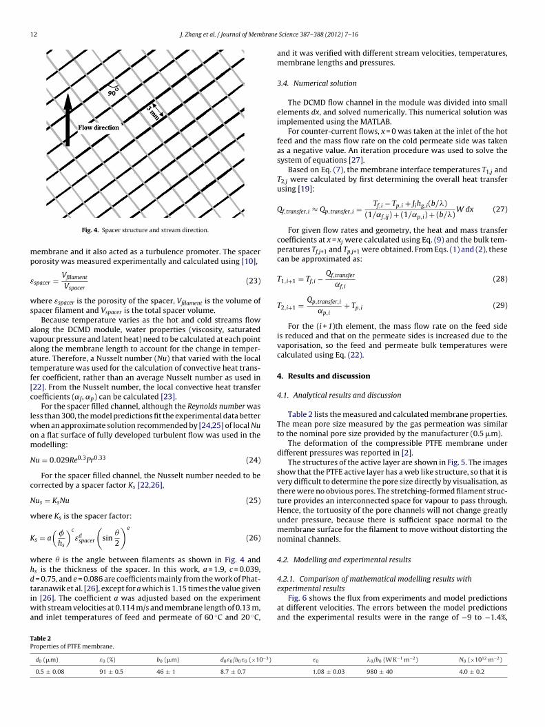
3.3. Modelling heat and mass transfer for spacer filled channel

The spacer used was 0.8 mm thick and composed of filaments(� = 0.4 mm), as shown in Fig. 4. The spacer was used to support the

employed DCMD process.

12 J. Zhang et al. / Journal of Membrane

mp

ε

ws

avaatf[c

lwom

N

c

N

w

K

whdtiwa

TP

Fig. 4. Spacer structure and stream direction.

embrane and it also acted as a turbulence promoter. The spacerorosity was measured experimentally and calculated using [10],

spacer = Vfilament

Vspacer(23)

here εspacer is the porosity of the spacer, Vfilament is the volume ofpacer filament and Vspacer is the total spacer volume.

Because temperature varies as the hot and cold streams flowlong the DCMD module, water properties (viscosity, saturatedapour pressure and latent heat) need to be calculated at each pointlong the membrane length to account for the change in temper-ture. Therefore, a Nusselt number (Nu) that varied with the localemperature was used for the calculation of convective heat trans-er coefficient, rather than an average Nusselt number as used in22]. From the Nusselt number, the local convective heat transferoefficients (˛f, ˛p) can be calculated [23].

For the spacer filled channel, although the Reynolds number wasess than 300, the model predictions fit the experimental data better

hen an approximate solution recommended by [24,25] of local Nun a flat surface of fully developed turbulent flow was used in theodelling:

u = 0.029Re0.3Pr0.33 (24)

For the spacer filled channel, the Nusselt number needed to beorrected by a spacer factor Ks [22,26],

us = KsNu (25)

here Ks is the spacer factor:

s = a(

�

hs

)c

εdspacer

(sin

�

2

)e

(26)

here � is the angle between filaments as shown in Fig. 4 ands is the thickness of the spacer. In this work, a = 1.9, c = 0.039,

= 0.75, and e = 0.086 are coefficients mainly from the work of Phat-

aranawik et al. [26], except for a which is 1.15 times the value givenn [26]. The coefficient a was adjusted based on the experiment

ith stream velocities at 0.114 m/s and membrane length of 0.13 m,nd inlet temperatures of feed and permeate of 60 ◦C and 20 ◦C,

able 2roperties of PTFE membrane.

d0 (�m) ε0 (%) b0 (�m) d0ε0/b0�0 (×10−3)

0.5 ± 0.08 91 ± 0.5 46 ± 1 8.7 ± 0.7

Science 387– 388 (2012) 7– 16

and it was verified with different stream velocities, temperatures,membrane lengths and pressures.

3.4. Numerical solution

The DCMD flow channel in the module was divided into smallelements dx, and solved numerically. This numerical solution wasimplemented using the MATLAB.

For counter-current flows, x = 0 was taken at the inlet of the hotfeed and the mass flow rate on the cold permeate side was takenas a negative value. An iteration procedure was used to solve thesystem of equations [27].

Based on Eq. (7), the membrane interface temperatures T1,j andT2,j were calculated by first determining the overall heat transferusing [19]:

Qf,transfer,i ≈ Qp,transfer,i = Tf,i − Tp,i + Jihg,i(b/�)(1/˛f,ij) + (1/˛p,i) + (b/�)

W dx (27)

For given flow rates and geometry, the heat and mass transfercoefficients at x = xj were calculated using Eq. (9) and the bulk tem-peratures Tf,j+1 and Tp,j+1 were obtained. From Eqs. (1) and (2), thesecan be approximated as:

T1,i+1 = Tf,i − Qf,transfer

˛f,i(28)

T2,i+1 = Qp,transfer,i

˛p,i+ Tp,i (29)

For the (i + 1)th element, the mass flow rate on the feed sideis reduced and that on the permeate sides is increased due to thevaporisation, so the feed and permeate bulk temperatures werecalculated using Eq. (22).

4. Results and discussion

4.1. Analytical results and discussion

Table 2 lists the measured and calculated membrane properties.The mean pore size measured by the gas permeation was similarto the nominal pore size provided by the manufacturer (0.5 �m).

The deformation of the compressible PTFE membrane underdifferent pressures was reported in [2].

The structures of the active layer are shown in Fig. 5. The imagesshow that the PTFE active layer has a web like structure, so that it isvery difficult to determine the pore size directly by visualisation, asthere were no obvious pores. The stretching-formed filament struc-ture provides an interconnected space for vapour to pass through.Hence, the tortuosity of the pore channels will not change greatlyunder pressure, because there is sufficient space normal to themembrane surface for the filament to move without distorting thenominal channels.

4.2. Modelling and experimental results

4.2.1. Comparison of mathematical modelling results with

experimental results

Fig. 6 shows the flux from experiments and model predictionsat different velocities. The errors between the model predictionsand the experimental results were in the range of −9 to −1.4%,

�0 �0/b0 (W K−1 m−2) N0 (×1012 m−2)

1.08 ± 0.03 980 ± 40 4.0 ± 0.2

J. Zhang et al. / Journal of Membrane Science 387– 388 (2012) 7– 16 13

a(

tte

ITra

F(

Fig. 5. Images for membrane structure.

nd the maximum absolute errors occurred at the lowest velocity0.056 m/s).

Fig. 7 shows the similar results as those in Fig. 6 at differentemperatures. The errors became larger at higher temperature, buthey remain in the range of −4.1 to −1.7%. The maximum absoluterror occurred at the highest temperature (70 ◦C).

The model was also assessed with various membrane lengths.n Fig. 8, results from modelling and experiments are presented.he errors between the predicted and experimental results were

andomly distributed in the range of −3.1 to 4.5%. The maximumbsolute error was 4.5% with a membrane length of 0.733 m.

ig. 6. Comparison between modelling and experimental flux at different velocitiesTfi = 60 ◦C, Tpi = 20 ◦C and Lmem = 130 mm).

Fig. 7. Comparison between modelling and experimental flux results at differenttemperatures (vf = vp = 0.114 m/s, Lmem = 130 mm).

Fig. 8 also shows that the flux decreases from 44.7 to11.1 L m−2 h−1 as the membrane length was increased from 0.050 mto 0.733 m at the same inlet temperature and velocity. The decreasein flux results from the temperature profile change along the mem-brane module. As water evaporates and transfers from the hot brineto the cold permeate, heat is also transferred from the brine tothe cold flow which reduces the temperature of the hot brine andincreases the temperature of the cold flow. Thus, as the membranelength is increased, the mean temperature difference between thehot and cold sides reduces, which leads to a decrease in averageflux. Therefore, the mass transfer coefficient (Eq. (19)) and dε/btrather than the flux are parameters to better characterise mem-brane performance as these do not vary with membrane length ortemperature.

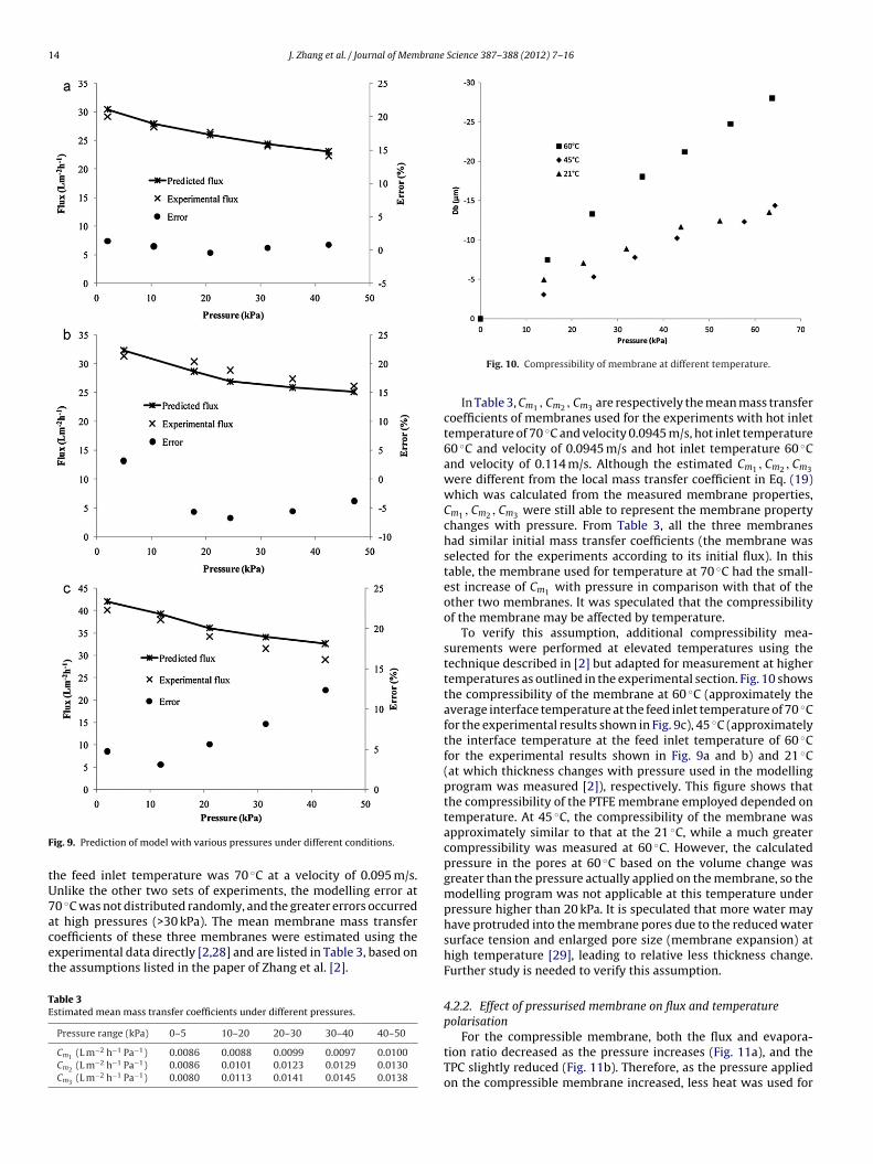
The modelling results were also compared with experimentalresults under different pressures, because the PTFE membrane usedwas compressible. Fig. 9 shows the experimental and predictedflux values based on data from [2], and errors between them undervarious pressures at different velocities and different hot inlet tem-peratures.

It can be found from Fig. 9 that the flux decreased as the pressureapplied on the membrane is increased. Furthermore, the agreementbetween the model predictions and experimental results was verygood when the feed inlet temperature was 60 ◦C, for which the error

was in the range of −2.1 to 1.3% at a velocity of 0.0945 m/s and−6.7 to 3.1% at a velocity of 0.114 m/s. This compares to an experi-mental variation of ±5%. The error was 3.1–12.4% (Fig. 9c) when

Fig. 8. Accuracy assessment with varied membrane lengths (Tfi = 60 ◦C, Tpi = 20 ◦C,vf = vp = 0.114 m/s).

14 J. Zhang et al. / Journal of Membrane Science 387– 388 (2012) 7– 16

F

tU7acet

TE

ig. 9. Prediction of model with various pressures under different conditions.

he feed inlet temperature was 70 ◦C at a velocity of 0.095 m/s.nlike the other two sets of experiments, the modelling error at0 ◦C was not distributed randomly, and the greater errors occurred

t high pressures (>30 kPa). The mean membrane mass transferoefficients of these three membranes were estimated using thexperimental data directly [2,28] and are listed in Table 3, based onhe assumptions listed in the paper of Zhang et al. [2].

able 3stimated mean mass transfer coefficients under different pressures.

Pressure range (kPa) 0–5 10–20 20–30 30–40 40–50

Cm1 (L m−2 h−1 Pa−1) 0.0086 0.0088 0.0099 0.0097 0.0100Cm2 (L m−2 h−1 Pa−1) 0.0086 0.0101 0.0123 0.0129 0.0130Cm3 (L m−2 h−1 Pa−1) 0.0080 0.0113 0.0141 0.0145 0.0138

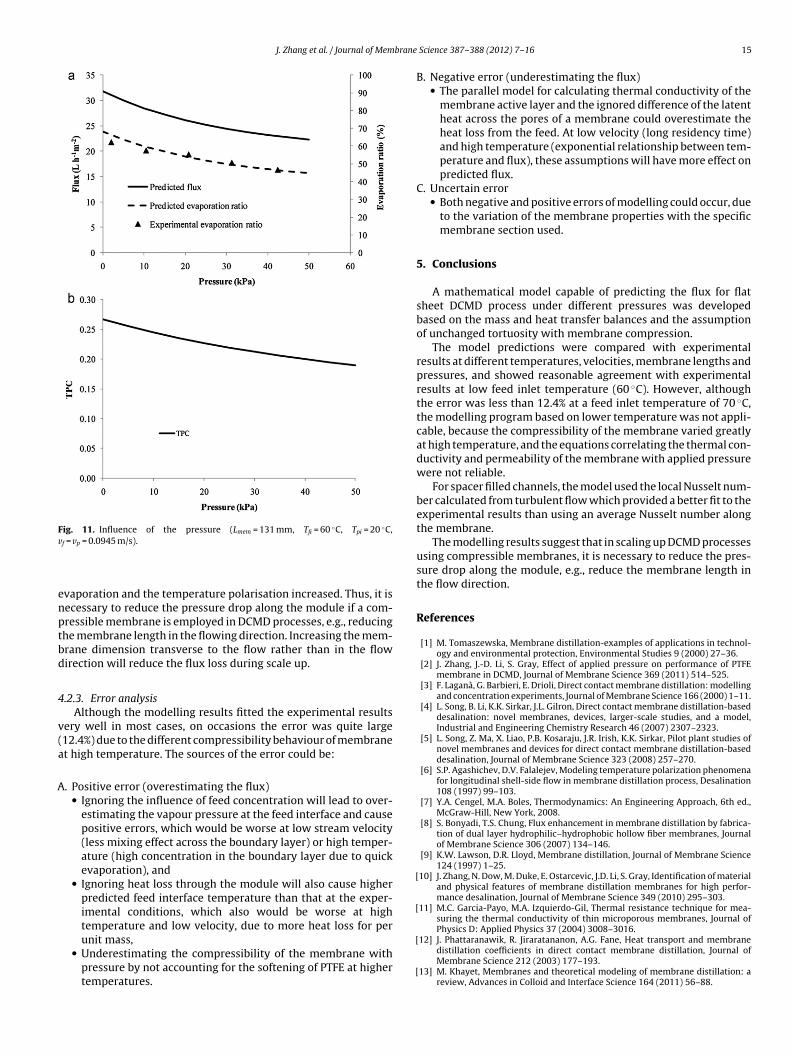
Fig. 10. Compressibility of membrane at different temperature.

In Table 3, Cm1 , Cm2 , Cm3 are respectively the mean mass transfercoefficients of membranes used for the experiments with hot inlettemperature of 70 ◦C and velocity 0.0945 m/s, hot inlet temperature60 ◦C and velocity of 0.0945 m/s and hot inlet temperature 60 ◦Cand velocity of 0.114 m/s. Although the estimated Cm1 , Cm2 , Cm3

were different from the local mass transfer coefficient in Eq. (19)which was calculated from the measured membrane properties,Cm1 , Cm2 , Cm3 were still able to represent the membrane propertychanges with pressure. From Table 3, all the three membraneshad similar initial mass transfer coefficients (the membrane wasselected for the experiments according to its initial flux). In thistable, the membrane used for temperature at 70 ◦C had the small-est increase of Cm1 with pressure in comparison with that of theother two membranes. It was speculated that the compressibilityof the membrane may be affected by temperature.

To verify this assumption, additional compressibility mea-surements were performed at elevated temperatures using thetechnique described in [2] but adapted for measurement at highertemperatures as outlined in the experimental section. Fig. 10 showsthe compressibility of the membrane at 60 ◦C (approximately theaverage interface temperature at the feed inlet temperature of 70 ◦Cfor the experimental results shown in Fig. 9c), 45 ◦C (approximatelythe interface temperature at the feed inlet temperature of 60 ◦Cfor the experimental results shown in Fig. 9a and b) and 21 ◦C(at which thickness changes with pressure used in the modellingprogram was measured [2]), respectively. This figure shows thatthe compressibility of the PTFE membrane employed depended ontemperature. At 45 ◦C, the compressibility of the membrane wasapproximately similar to that at the 21 ◦C, while a much greatercompressibility was measured at 60 ◦C. However, the calculatedpressure in the pores at 60 ◦C based on the volume change wasgreater than the pressure actually applied on the membrane, so themodelling program was not applicable at this temperature underpressure higher than 20 kPa. It is speculated that more water mayhave protruded into the membrane pores due to the reduced watersurface tension and enlarged pore size (membrane expansion) athigh temperature [29], leading to relative less thickness change.Further study is needed to verify this assumption.

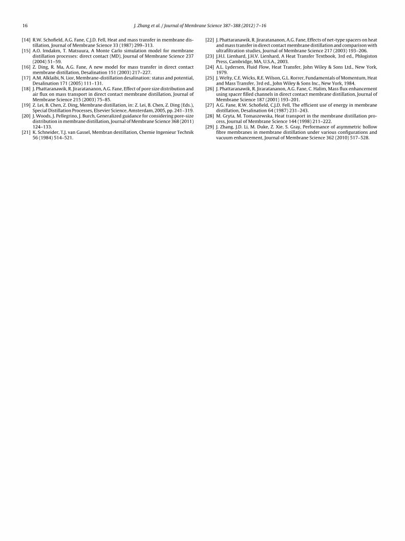
4.2.2. Effect of pressurised membrane on flux and temperaturepolarisation

For the compressible membrane, both the flux and evapora-tion ratio decreased as the pressure increases (Fig. 11a), and theTPC slightly reduced (Fig. 11b). Therefore, as the pressure appliedon the compressible membrane increased, less heat was used for

J. Zhang et al. / Journal of Membrane

Fig. 11. Influence of the pressure (Lmem = 131 mm, Tfi = 60 ◦C, Tpi = 20 ◦C,v

enptbd

4

v(a

A

[

[

f = vp = 0.0945 m/s).

vaporation and the temperature polarisation increased. Thus, it isecessary to reduce the pressure drop along the module if a com-ressible membrane is employed in DCMD processes, e.g., reducinghe membrane length in the flowing direction. Increasing the mem-rane dimension transverse to the flow rather than in the flowirection will reduce the flux loss during scale up.

.2.3. Error analysisAlthough the modelling results fitted the experimental results

ery well in most cases, on occasions the error was quite large12.4%) due to the different compressibility behaviour of membranet high temperature. The sources of the error could be:

. Positive error (overestimating the flux)• Ignoring the influence of feed concentration will lead to over-

estimating the vapour pressure at the feed interface and causepositive errors, which would be worse at low stream velocity(less mixing effect across the boundary layer) or high temper-ature (high concentration in the boundary layer due to quickevaporation), and

• Ignoring heat loss through the module will also cause higherpredicted feed interface temperature than that at the exper-imental conditions, which also would be worse at high

temperature and low velocity, due to more heat loss for perunit mass,

• Underestimating the compressibility of the membrane withpressure by not accounting for the softening of PTFE at highertemperatures.

[

[

Science 387– 388 (2012) 7– 16 15

B. Negative error (underestimating the flux)• The parallel model for calculating thermal conductivity of the

membrane active layer and the ignored difference of the latentheat across the pores of a membrane could overestimate theheat loss from the feed. At low velocity (long residency time)and high temperature (exponential relationship between tem-perature and flux), these assumptions will have more effect onpredicted flux.

C. Uncertain error• Both negative and positive errors of modelling could occur, due

to the variation of the membrane properties with the specificmembrane section used.

5. Conclusions

A mathematical model capable of predicting the flux for flatsheet DCMD process under different pressures was developedbased on the mass and heat transfer balances and the assumptionof unchanged tortuosity with membrane compression.

The model predictions were compared with experimentalresults at different temperatures, velocities, membrane lengths andpressures, and showed reasonable agreement with experimentalresults at low feed inlet temperature (60 ◦C). However, althoughthe error was less than 12.4% at a feed inlet temperature of 70 ◦C,the modelling program based on lower temperature was not appli-cable, because the compressibility of the membrane varied greatlyat high temperature, and the equations correlating the thermal con-ductivity and permeability of the membrane with applied pressurewere not reliable.

For spacer filled channels, the model used the local Nusselt num-ber calculated from turbulent flow which provided a better fit to theexperimental results than using an average Nusselt number alongthe membrane.

The modelling results suggest that in scaling up DCMD processesusing compressible membranes, it is necessary to reduce the pres-sure drop along the module, e.g., reduce the membrane length inthe flow direction.

References

[1] M. Tomaszewska, Membrane distillation-examples of applications in technol-ogy and environmental protection, Environmental Studies 9 (2000) 27–36.

[2] J. Zhang, J.-D. Li, S. Gray, Effect of applied pressure on performance of PTFEmembrane in DCMD, Journal of Membrane Science 369 (2011) 514–525.

[3] F. Laganà, G. Barbieri, E. Drioli, Direct contact membrane distillation: modellingand concentration experiments, Journal of Membrane Science 166 (2000) 1–11.

[4] L. Song, B. Li, K.K. Sirkar, J.L. Gilron, Direct contact membrane distillation-baseddesalination: novel membranes, devices, larger-scale studies, and a model,Industrial and Engineering Chemistry Research 46 (2007) 2307–2323.

[5] L. Song, Z. Ma, X. Liao, P.B. Kosaraju, J.R. Irish, K.K. Sirkar, Pilot plant studies ofnovel membranes and devices for direct contact membrane distillation-baseddesalination, Journal of Membrane Science 323 (2008) 257–270.

[6] S.P. Agashichev, D.V. Falalejev, Modeling temperature polarization phenomenafor longitudinal shell-side flow in membrane distillation process, Desalination108 (1997) 99–103.

[7] Y.A. Cengel, M.A. Boles, Thermodynamics: An Engineering Approach, 6th ed.,McGraw-Hill, New York, 2008.

[8] S. Bonyadi, T.S. Chung, Flux enhancement in membrane distillation by fabrica-tion of dual layer hydrophilic–hydrophobic hollow fiber membranes, Journalof Membrane Science 306 (2007) 134–146.

[9] K.W. Lawson, D.R. Lloyd, Membrane distillation, Journal of Membrane Science124 (1997) 1–25.

10] J. Zhang, N. Dow, M. Duke, E. Ostarcevic, J.D. Li, S. Gray, Identification of materialand physical features of membrane distillation membranes for high perfor-mance desalination, Journal of Membrane Science 349 (2010) 295–303.

11] M.C. Garcia-Payo, M.A. Izquierdo-Gil, Thermal resistance technique for mea-suring the thermal conductivity of thin microporous membranes, Journal ofPhysics D: Applied Physics 37 (2004) 3008–3016.

12] J. Phattaranawik, R. Jiraratananon, A.G. Fane, Heat transport and membranedistillation coefficients in direct contact membrane distillation, Journal ofMembrane Science 212 (2003) 177–193.

13] M. Khayet, Membranes and theoretical modeling of membrane distillation: areview, Advances in Colloid and Interface Science 164 (2011) 56–88.

1 brane

[

[

[

[

[

[

[

[

[

[

[

[

[

[

6 J. Zhang et al. / Journal of Mem

14] R.W. Schofield, A.G. Fane, C.J.D. Fell, Heat and mass transfer in membrane dis-tillation, Journal of Membrane Science 33 (1987) 299–313.

15] A.O. Imdakm, T. Matsuura, A Monte Carlo simulation model for membranedistillation processes: direct contact (MD), Journal of Membrane Science 237(2004) 51–59.

16] Z. Ding, R. Ma, A.G. Fane, A new model for mass transfer in direct contactmembrane distillation, Desalination 151 (2003) 217–227.

17] A.M. Alklaibi, N. Lior, Membrane-distillation desalination: status and potential,Desalination 171 (2005) 111–131.

18] J. Phattaranawik, R. Jiraratananon, A.G. Fane, Effect of pore size distribution andair flux on mass transport in direct contact membrane distillation, Journal ofMembrane Science 215 (2003) 75–85.

19] Z. Lei, B. Chen, Z. Ding, Membrane distillation, in: Z. Lei, B. Chen, Z. Ding (Eds.),Special Distillation Processes, Elsevier Science, Amsterdam, 2005, pp. 241–319.

20] J. Woods, J. Pellegrino, J. Burch, Generalized guidance for considering pore-sizedistribution in membrane distillation, Journal of Membrane Science 368 (2011)124–133.

21] K. Schneider, T.J. van Gassel, Membran destillation, Chemie Ingenieur Technik56 (1984) 514–521.

[

[

Science 387– 388 (2012) 7– 16

22] J. Phattaranawik, R. Jiraratananon, A.G. Fane, Effects of net-type spacers on heatand mass transfer in direct contact membrane distillation and comparison withultrafiltration studies, Journal of Membrane Science 217 (2003) 193–206.

23] J.H.I. Lienhard, J.H.V. Lienhard, A Heat Transfer Textbook, 3rd ed., PhlogistonPress, Cambridge, MA, U.S.A., 2003.

24] A.L. Lydersen, Fluid Flow, Heat Transfer, John Wiley & Sons Ltd., New York,1979.

25] J. Welty, C.E. Wicks, R.E. Wilson, G.L. Rorrer, Fundamentals of Momentum, Heatand Mass Transfer, 3rd ed., John Wiley & Sons Inc., New York, 1984.

26] J. Phattaranawik, R. Jiraratananon, A.G. Fane, C. Halim, Mass flux enhancementusing spacer filled channels in direct contact membrane distillation, Journal ofMembrane Science 187 (2001) 193–201.

27] A.G. Fane, R.W. Schofield, C.J.D. Fell, The efficient use of energy in membranedistillation, Desalination 64 (1987) 231–243.

28] M. Gryta, M. Tomaszewska, Heat transport in the membrane distillation pro-cess, Journal of Membrane Science 144 (1998) 211–222.

29] J. Zhang, J.D. Li, M. Duke, Z. Xie, S. Gray, Performance of asymmetric hollowfibre membranes in membrane distillation under various configurations andvacuum enhancement, Journal of Membrane Science 362 (2010) 517–528.