DCM: Advanced issues Klaas Enno Stephan Laboratory for Social & Neural Systems Research Institute for Empirical Research in Economics University of Zurich

DCM: Advanced issues

Klaas Enno Stephan

Laboratory for Social & Neural Systems Research Institute for Empirical Research in EconomicsUniversity of Zurich

Functional Imaging Laboratory (FIL)Wellcome Trust Centre for NeuroimagingUniversity College London

Methods & Models for fMRI data analysis17 December 2008

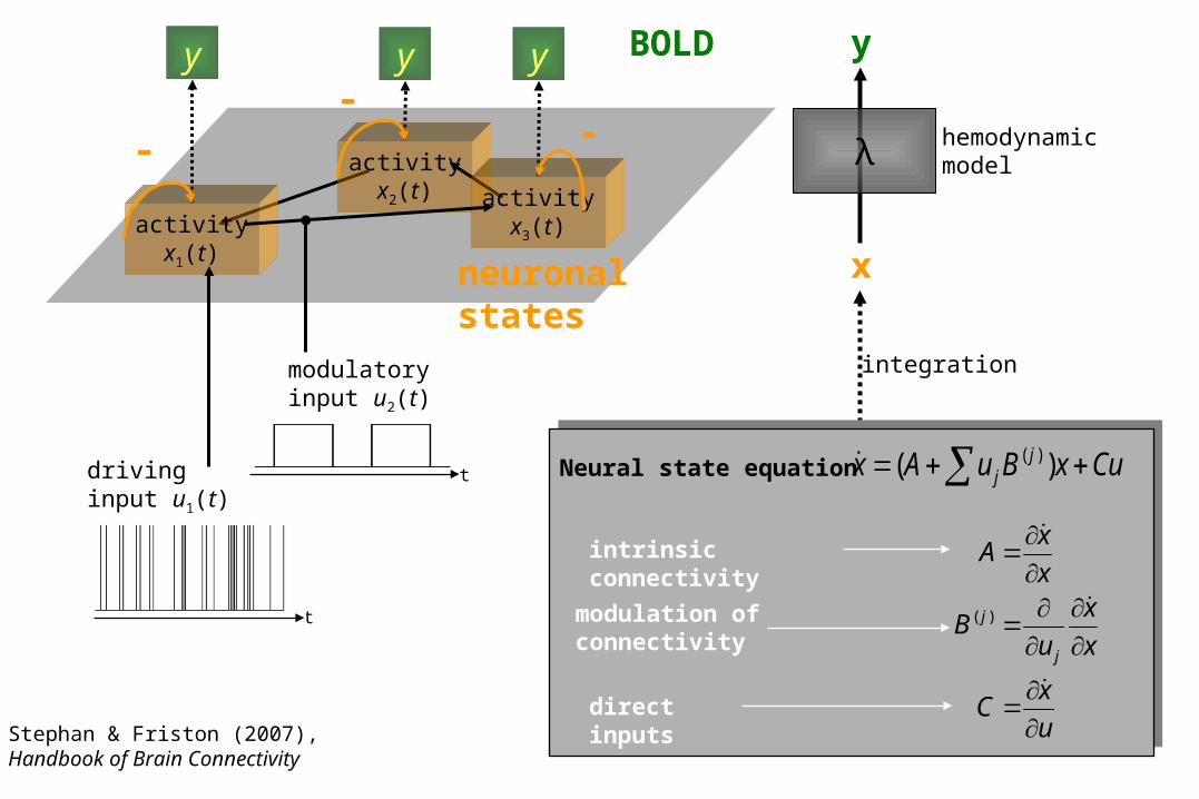
intrinsic connectivity

direct inputs

modulation ofconnectivity

Neural state equation CuxBuAx jj )( )(

u

xC

x

x

uB

x

xA

j

j

)(

hemodynamicmodelλ

x

y

integration

BOLDyyy

activityx1(t)

activityx2(t) activity

x3(t)

neuronalstates

t

drivinginput u1(t)

modulatoryinput u2(t)

t

Stephan & Friston (2007),Handbook of Brain Connectivity

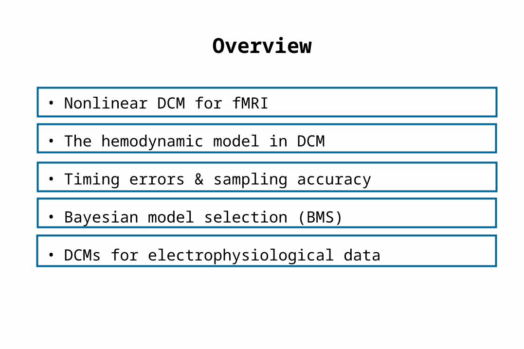
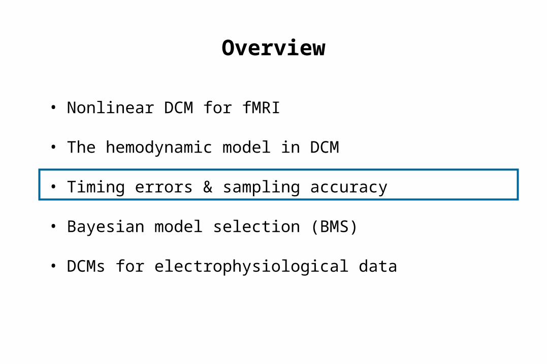
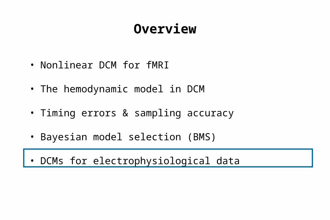
Overview

• Nonlinear DCM for fMRI

• The hemodynamic model in DCM

• Timing errors & sampling accuracy

• Bayesian model selection (BMS)

• DCMs for electrophysiological data

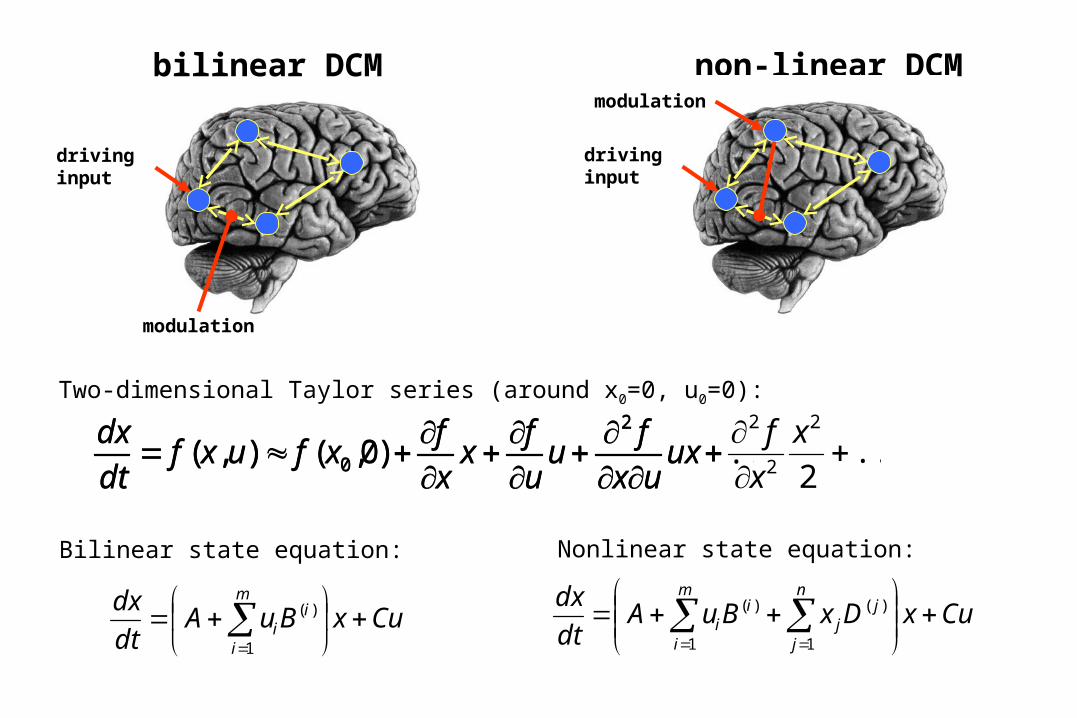
bilinear DCM

CuxDxBuAdt

dx m

i

n

j

jj

ii

1 1

)()(CuxBuA

dt

dx m

i

ii

1

)(

Bilinear state equation:

driving input

modulation

non-linear DCM

driving input

modulation

...)0,(),(2

0

uxux

fu

u

fx

x

fxfuxf

dt

dx

Two-dimensional Taylor series (around x0=0, u0=0):

Nonlinear state equation:

...2

)0,(),(2

2

22

0

x

x

fux

ux

fu

u

fx

x

fxfuxf

dt

dx

0 10 20 30 40 50 60 70 80 90 100

0

0.1

0.2

0.3

0.4

0 10 20 30 40 50 60 70 80 90 100

0

0.2

0.4

0.6

0 10 20 30 40 50 60 70 80 90 100

0

0.1

0.2

0.3

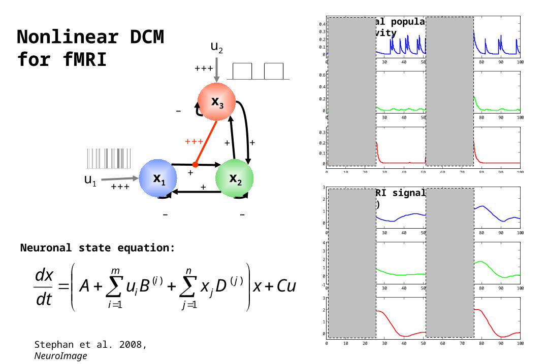
Neural population activity

0 10 20 30 40 50 60 70 80 90 100

0

1

2

3

0 10 20 30 40 50 60 70 80 90 100-1

0

1

2

3

4

0 10 20 30 40 50 60 70 80 90 100

0

1

2

3

fMRI signal change (%)

x1 x2u1

x3

u2

–

– –

++

++++

+++

+++

+

CuxDxBuAdt

dx n

j

jj

m

i

ii

1

)(

1

)(

Neuronal state equation:

Stephan et al. 2008, NeuroImage

Nonlinear DCMfor fMRI

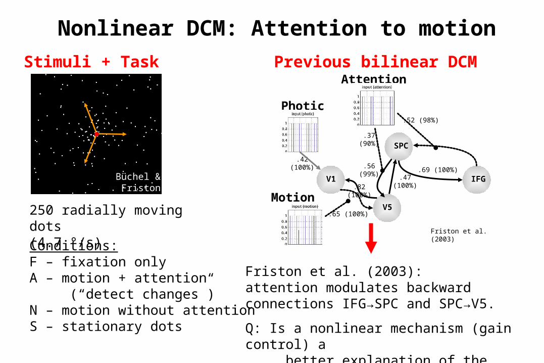
Nonlinear DCM: Attention to motion

V1 IFG

V5

SPC

Motion

Photic

Attention

.82(100%)

.42(100%)

.37(90%)

.69 (100%).47

(100%)

.65 (100%)

.52 (98%)

.56(99%)

Stimuli + Task

250 radially moving dots (4.7 °/s)

Conditions:F – fixation onlyA – motion + attention (“detect changes”)N – motion without attentionS – stationary dots

Previous bilinear DCM

Friston et al. (2003)

Friston et al. (2003):attention modulates backward connections IFG→SPC and SPC→V5.

Q: Is a nonlinear mechanism (gain control) a better explanation of the data?

Büchel & Friston (1997)

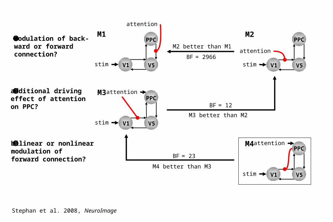
modulation of back-ward or forward connection?

additional drivingeffect of attentionon PPC?

bilinear or nonlinearmodulation offorward connection?

V1 V5stim

PPCM2

attention

V1 V5stim

PPCM1

attention

V1 V5stim

PPCM3attention

V1 V5stim

PPCM4attention

BF = 2966

M2 better than M1

M3 better than M2

BF = 12

M4 better than M3

BF = 23


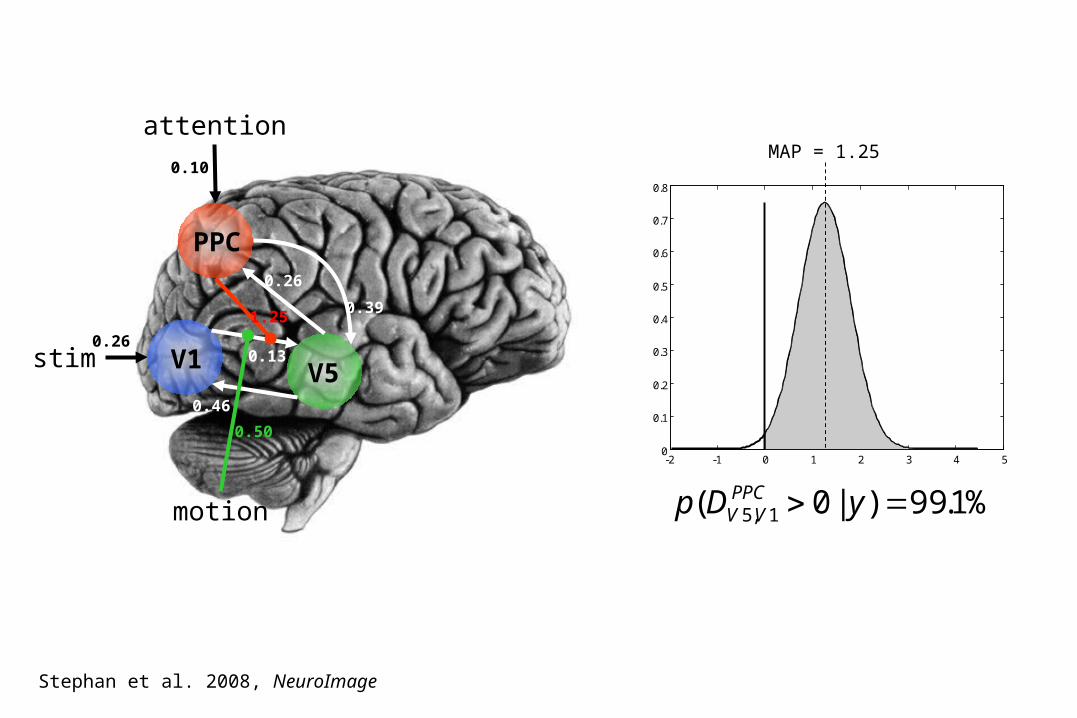
V1 V5stim

PPC

attention

motion

-2 -1 0 1 2 3 4 50

0.1

0.2

0.3

0.4

0.5

0.6

0.7

0.8

%1.99)|0( 1,5 yDp PPCVV

1.25

0.13

0.46

0.39

0.26

0.50

0.26

0.10MAP = 1.25


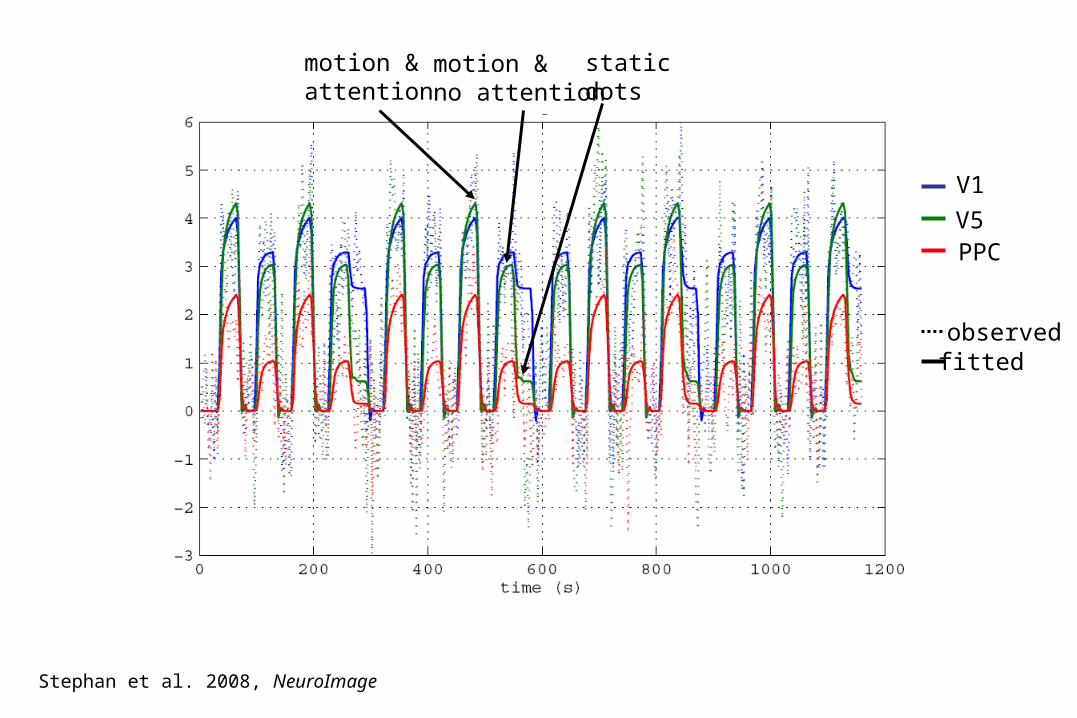
V1

V5PPC

observedfitted

motion &attention

motion &no attention

static dots


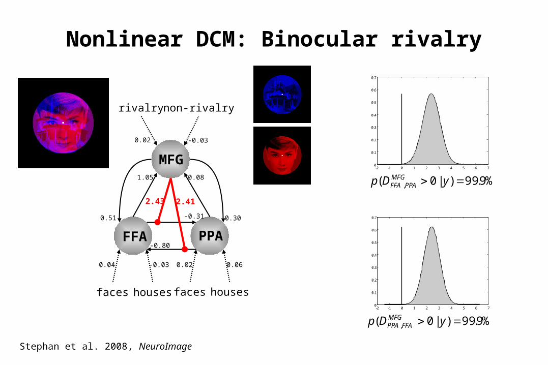
FFA PPA

MFG

-0.80

-0.31

faces houses faces houses

rivalry non-rivalry

1.05 0.08

0.300.51

2.43 2.41

0.04 -0.03 0.02 0.06

0.02 -0.03

-2 -1 0 1 2 3 4 5 6 70

0.1

0.2

0.3

0.4

0.5

0.6

0.7

-2 -1 0 1 2 3 4 5 6 70

0.1

0.2

0.3

0.4

0.5

0.6

0.7

%9.99)|0( , yDp MFGFFAPPA

%9.99)|0( , yDp MFGPPAFFA

Nonlinear DCM: Binocular rivalry


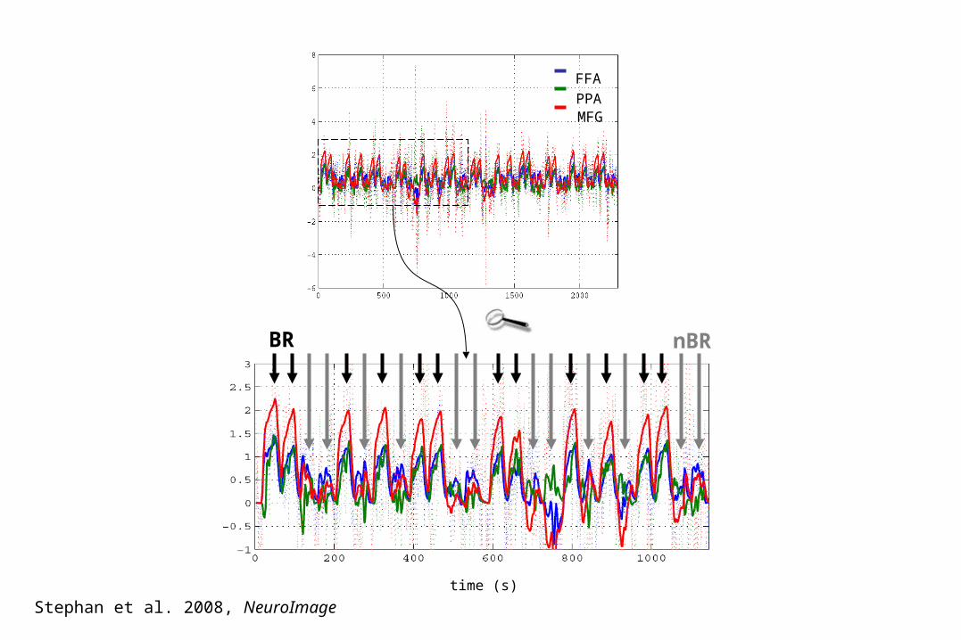
BR nBR

FFA

PPAMFG

time (s)


Overview






sf

tionflow induc

(rCBF)

s

v

stimulus functions

v

q q/vvEf,EEfqτ /α

dHbchanges in

100 )( /αvfvτ

volumechanges in

1

f

q

)1(

fγsxs

signalryvasodilato

u

s

CuxBuAdt

dx m

j

jj

1

)(

t

neural state equation

1

3.4

111),(

3

002

001

32100

k

TEErk

TEEk

vkv

qkqkV

S

Svq

hemodynamic state equationsf

Balloon model

BOLD signal change equation

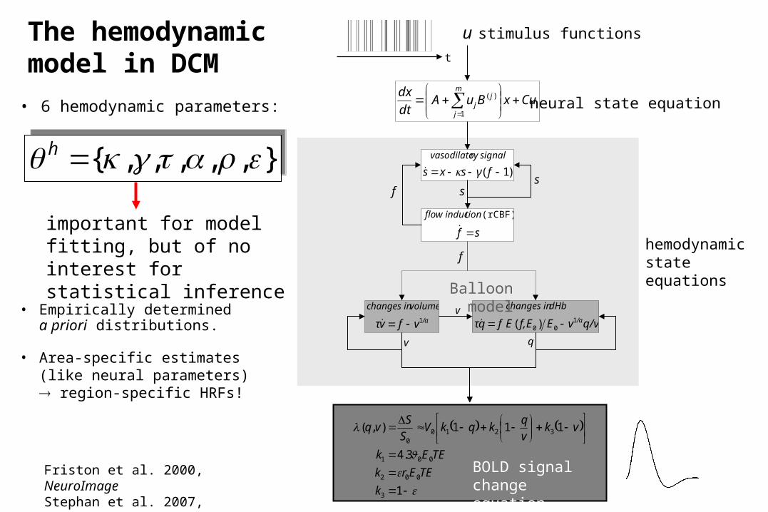
},,,,,{ h},,,,,{ h

important for model fitting, but of no interest for statistical inference

• 6 hemodynamic parameters:

• Empirically determineda priori distributions.

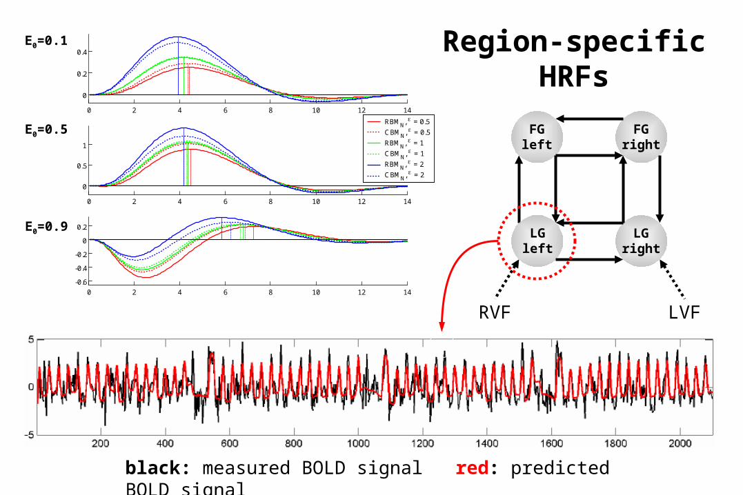
• Area-specific estimates (like neural parameters) region-specific HRFs!

The hemodynamic model in DCM

Friston et al. 2000, NeuroImageStephan et al. 2007, NeuroImage

0 2 4 6 8 10 12 14

0

0.2

0.4

0 2 4 6 8 10 12 14

0

0.5

1

0 2 4 6 8 10 12 14

-0.6

-0.4

-0.2

0

0.2

RBMN

, = 0.5

CBMN

, = 0.5

RBMN

, = 1

CBMN

, = 1

RBMN

, = 2

CBMN

, = 2

LGleft

LGright

RVF LVF

FGright

FGleft

black: measured BOLD signal red: predicted BOLD signal

Region-specific HRFs

E0=0.1

E0=0.5

E0=0.9

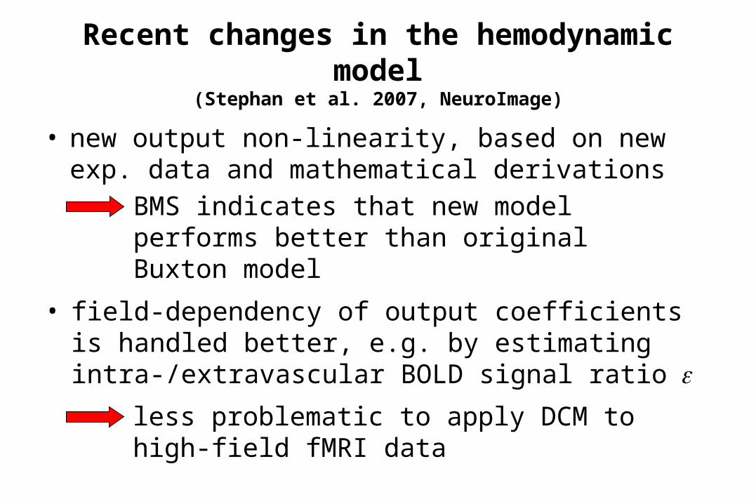
Recent changes in the hemodynamic model

(Stephan et al. 2007, NeuroImage)

• new output non-linearity, based on new exp. data and mathematical derivations

less problematic to apply DCM to high-field fMRI data

• field-dependency of output coefficients is handled better, e.g. by estimating intra-/extravascular BOLD signal ratio

BMS indicates that new model performs better than original Buxton model

5 10 15 20 25 30 35 40

5

10

15

20

25

30

35

40

-1

-0.8

-0.6

-0.4

-0.2

0

0.2

0.4

0.6

0.8

1

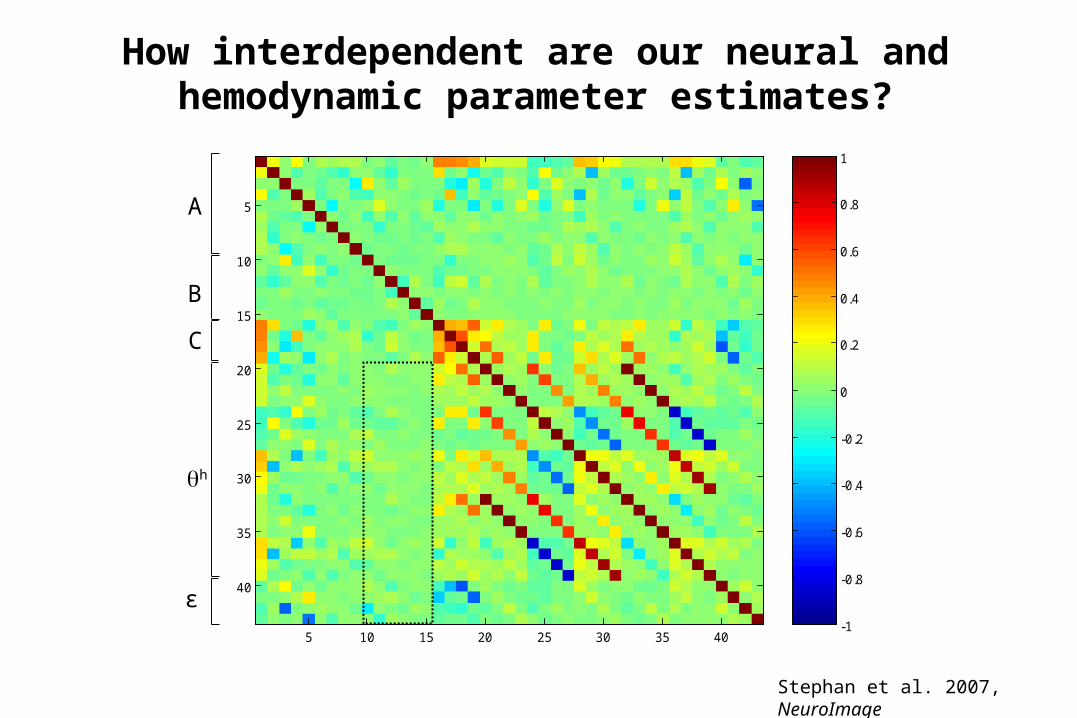
A

B

C

h

ε

How interdependent are our neural and hemodynamic parameter estimates?


Overview






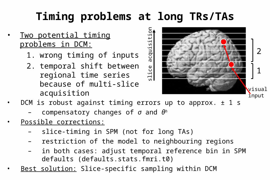
Timing problems at long TRs/TAs

• Two potential timing problems in DCM:

1. wrong timing of inputs2. temporal shift between

regional time series because of multi-slice acquisition

• DCM is robust against timing errors up to approx. ± 1 s – compensatory changes of σ and θh

• Possible corrections:– slice-timing in SPM (not for long TAs)– restriction of the model to neighbouring regions– in both cases: adjust temporal reference bin in SPM defaults

(defaults.stats.fmri.t0)• Best solution: Slice-specific sampling within DCM

1

2

slic

e a

cquis

itio

n

visualinput

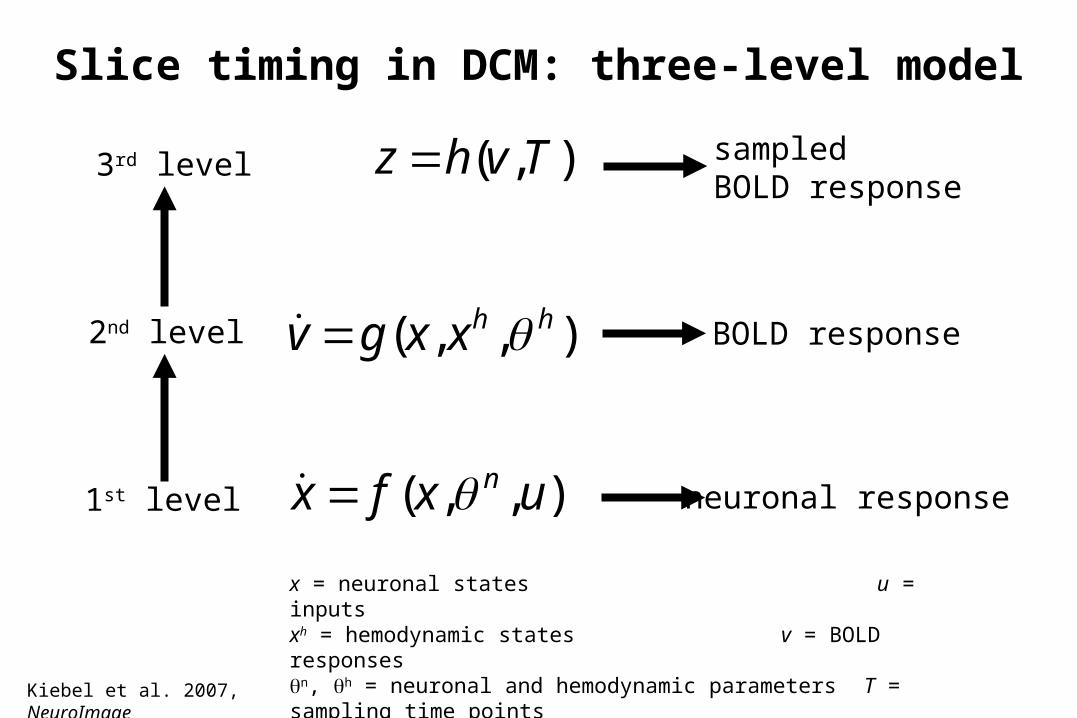
Slice timing in DCM: three-level model

),,( hhxxgv

),( Tvhz

),,( uxfx n

3rd level

2nd level

1st level

sampled BOLD response

BOLD response

neuronal response

x = neuronal states u = inputsxh = hemodynamic states v = BOLD responsesn, h = neuronal and hemodynamic parameters T = sampling time points

Kiebel et al. 2007, NeuroImage

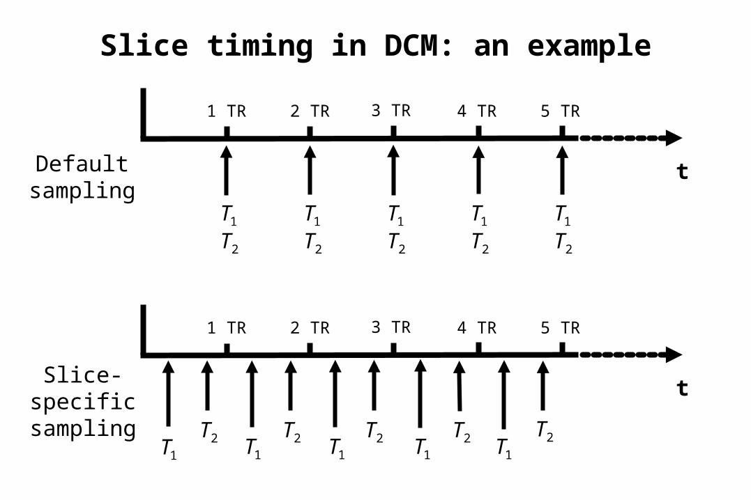
Slice timing in DCM: an example

t

1 TR 2 TR 3 TR 4 TR 5 TR

t

1 TR 2 TR 3 TR 4 TR 5 TR

Defaultsampling

Slice-specific sampling

1T

2T1T

2T1T

2T1T

2T1T

2T

1T 1T 1T 1T 1T2T 2T 2T 2T 2T

Overview






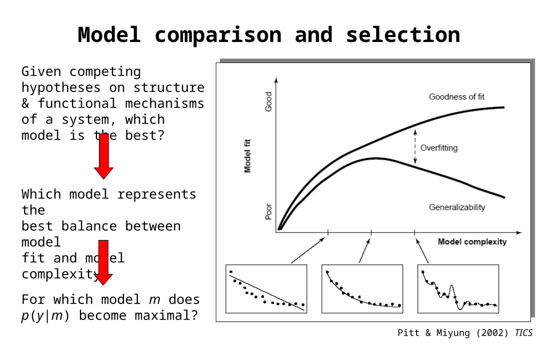
Model comparison and selection

Given competing hypotheses on structure & functional mechanisms of a system, which model is the best?

For which model m does p(y|m) become maximal?

Which model represents thebest balance between model fit and model complexity?

Pitt & Miyung (2002) TICS

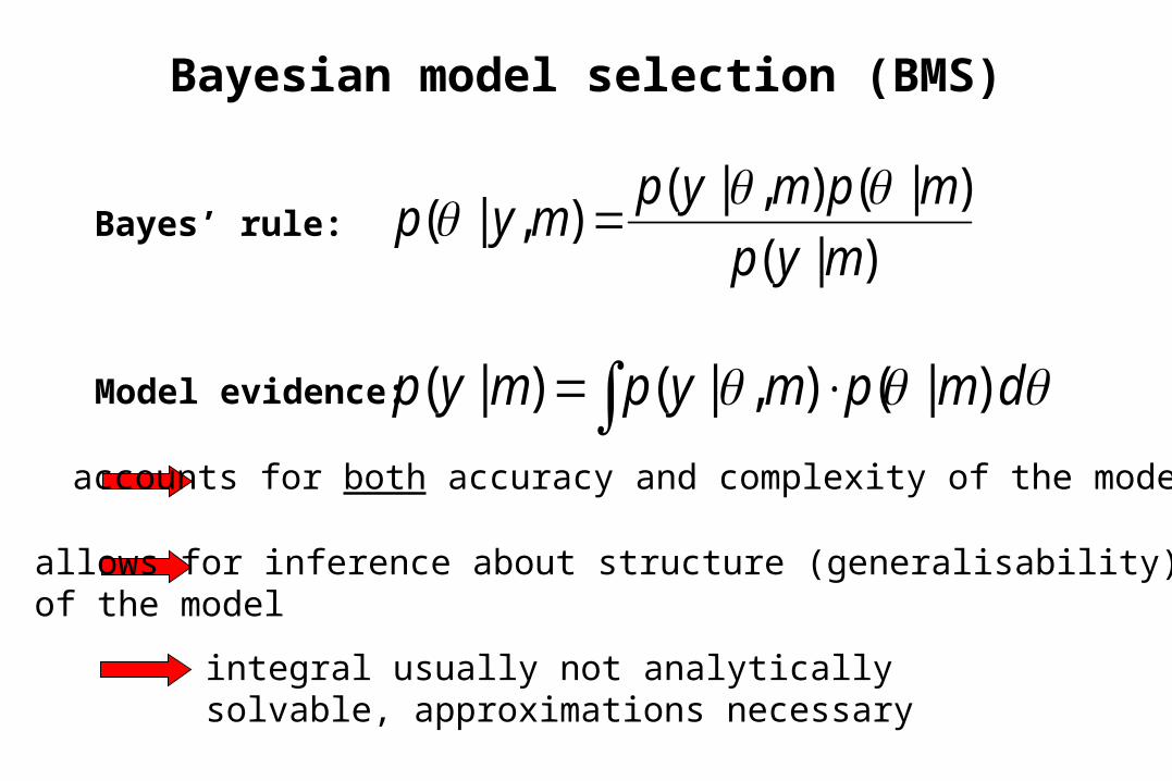
dmpmypmyp )|(),|()|( Model evidence:

Bayesian model selection (BMS)

)|(

)|(),|(),|(

myp

mpmypmyp

Bayes’ rule:

accounts for both accuracy and complexity of the model

allows for inference about structure (generalisability)of the model

integral usually not analytically solvable, approximations necessary

dmpmypmyp )|(),|()|(

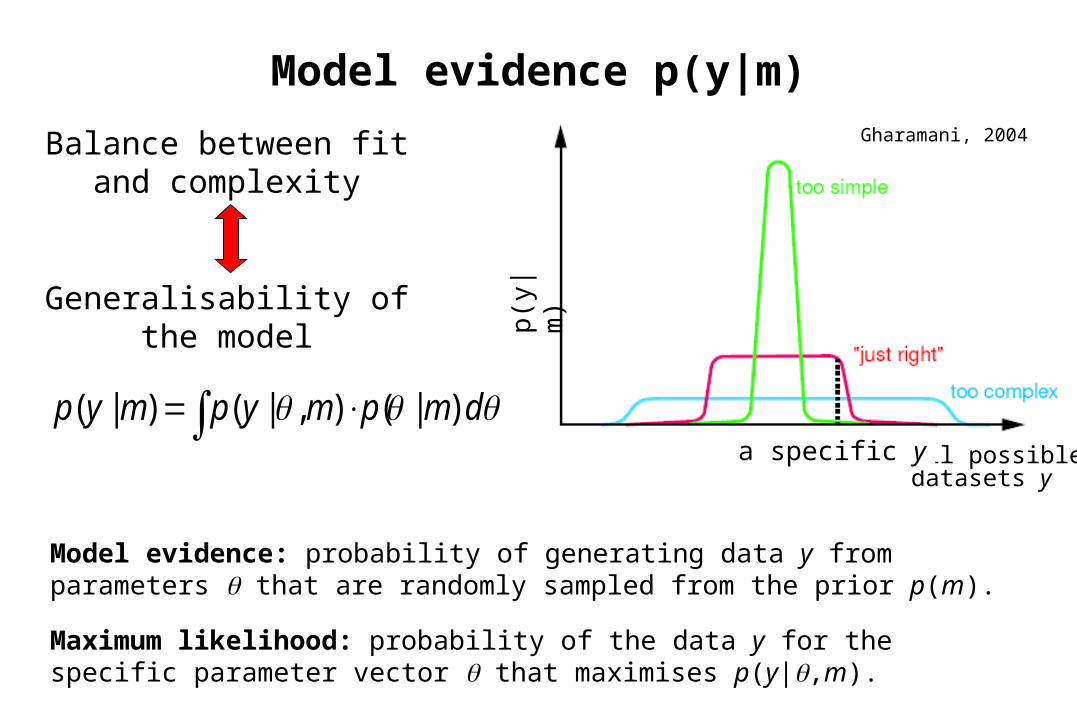
Model evidence p(y|m)Gharamani, 2004

p(y

|m

)

all possible datasets y

a specific y

Balance between fit and complexity

Generalisability of the model

Model evidence: probability of generating data y from parameters that are randomly sampled from the prior p(m).

Maximum likelihood: probability of the data y for the specific parameter vector that maximises p(y|,m).

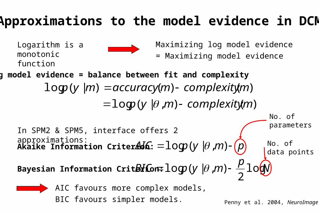
pmypAIC ),|(log

Logarithm is a monotonic function

Maximizing log model evidence= Maximizing model evidence

)(),|(log

)()( )|(log

mcomplexitymyp

mcomplexitymaccuracymyp

In SPM2 & SPM5, interface offers 2 approximations:

Np

mypBIC log2

),|(log

Akaike Information Criterion:

Bayesian Information Criterion:

Log model evidence = balance between fit and complexity

Penny et al. 2004, NeuroImage

Approximations to the model evidence in DCM

No. of parameters

No. ofdata points

AIC favours more complex models,BIC favours simpler models.

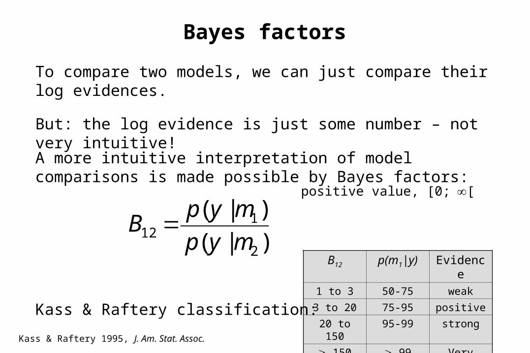
Bayes factors

)|(

)|(

2

112 myp

mypB

positive value, [0;[

But: the log evidence is just some number – not very intuitive!

A more intuitive interpretation of model comparisons is made possible by Bayes factors:

To compare two models, we can just compare their log evidences.

B12 p(m1|y) Evidence

1 to 3 50-75 weak

3 to 20 75-95 positive

20 to 150 95-99 strong

150 99 Very strong

Kass & Raftery classification:

Kass & Raftery 1995, J. Am. Stat. Assoc.

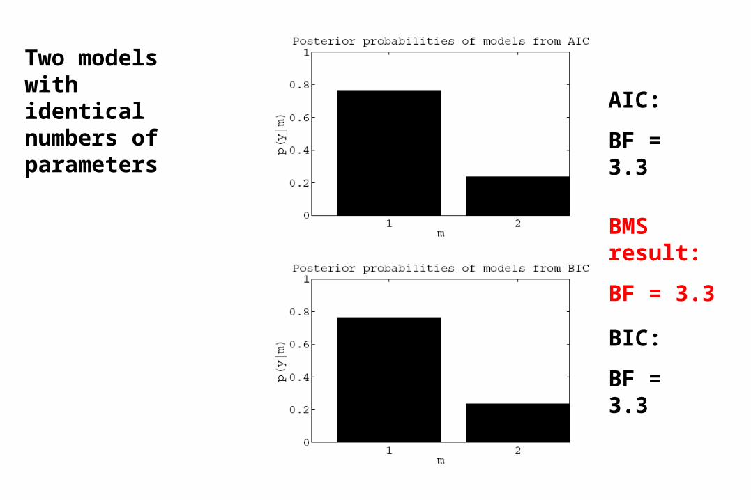
AIC:

BF = 3.3

BIC:

BF = 3.3

BMS result:

BF = 3.3

Two models with identical numbers of parameters

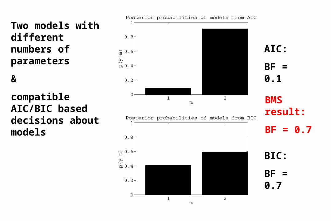
AIC:

BF = 0.1

BIC:

BF = 0.7

BMS result:

BF = 0.7

Two models with different numbers of parameters

&

compatible AIC/BIC based decisions about models

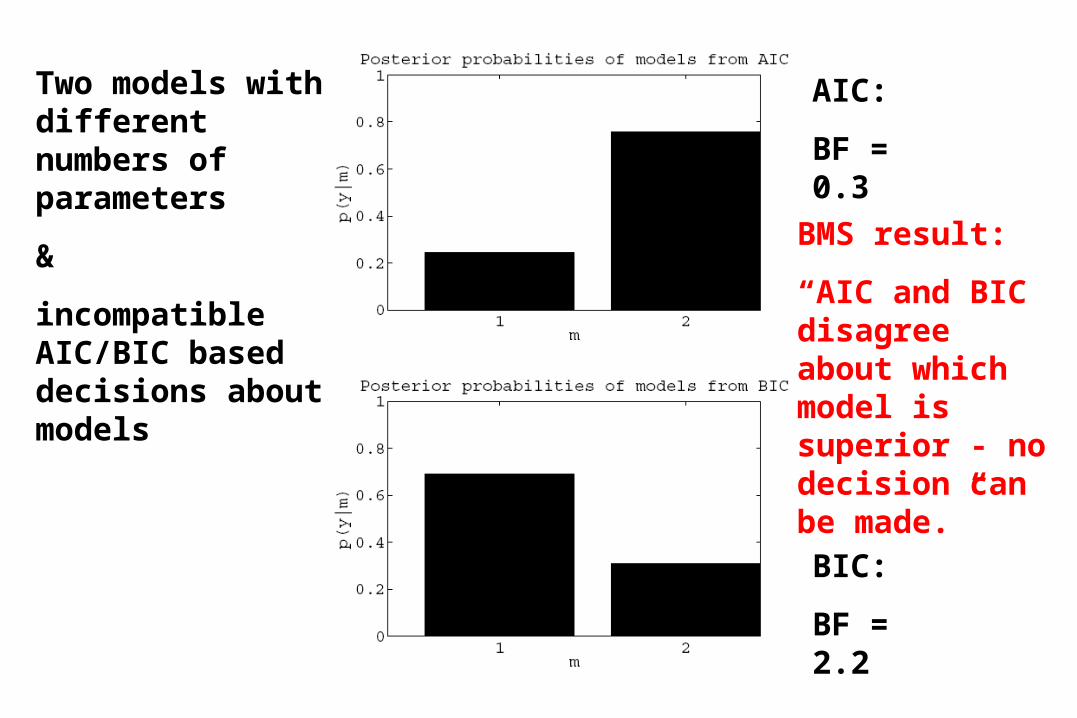
AIC:

BF = 0.3

BIC:

BF = 2.2

BMS result:

“AIC and BIC disagree about which model is superior - no decision can be made.”

Two models with different numbers of parameters

&

incompatible AIC/BIC based decisions about models

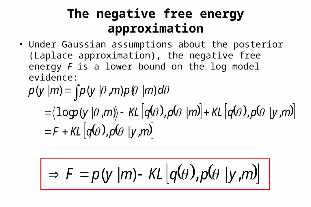
The negative free energy approximation

• Under Gaussian assumptions about the posterior (Laplace approximation), the negative free energy F is a lower bound on the log model evidence:

mypqKLF

mypqKLmpqKLmyp

dmpmypmyp

,|,

,|,|,),|(log

)|(),|()|(

mypqKLmypF ,|,)|(

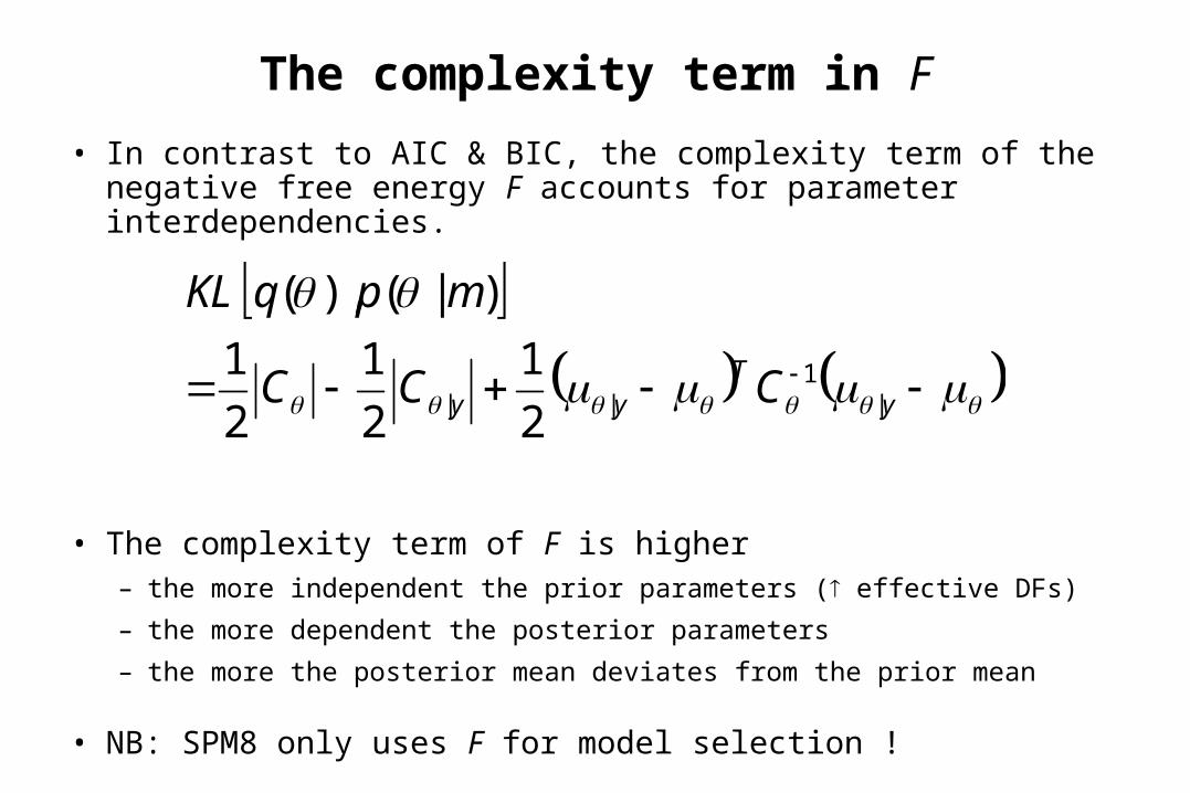
The complexity term in F

• In contrast to AIC & BIC, the complexity term of the negative free energy F accounts for parameter interdependencies.

• The complexity term of F is higher– the more independent the prior parameters ( effective DFs)

– the more dependent the posterior parameters

– the more the posterior mean deviates from the prior mean

• NB: SPM8 only uses F for model selection !

y

Tyy CCC

mpqKL

|1

|| 2

1

2

1

2

1

)|(),(

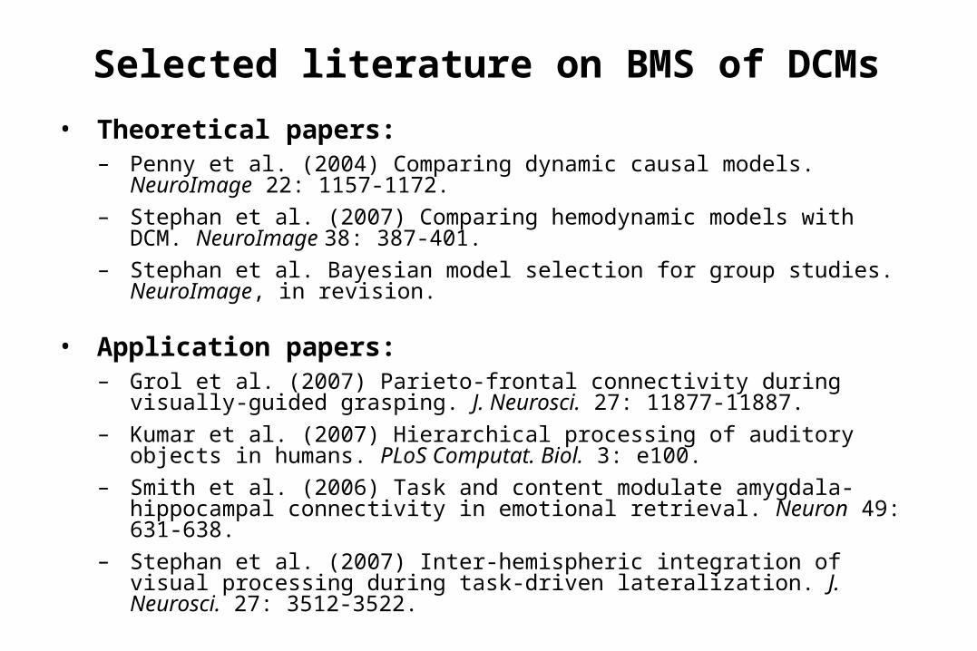
Selected literature on BMS of DCMs

• Theoretical papers:– Penny et al. (2004) Comparing dynamic causal models. NeuroImage 22:

1157-1172.

– Stephan et al. (2007) Comparing hemodynamic models with DCM. NeuroImage 38: 387-401.

– Stephan et al. Bayesian model selection for group studies. NeuroImage, in revision.

• Application papers:– Grol et al. (2007) Parieto-frontal connectivity during visually-guided

grasping. J. Neurosci. 27: 11877-11887.

– Kumar et al. (2007) Hierarchical processing of auditory objects in humans. PLoS Computat. Biol. 3: e100.

– Smith et al. (2006) Task and content modulate amygdala-hippocampal connectivity in emotional retrieval. Neuron 49: 631-638.

– Stephan et al. (2007) Inter-hemispheric integration of visual processing during task-driven lateralization. J. Neurosci. 27: 3512-3522.

Overview






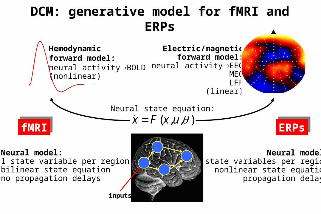
),,( uxFx Neural state equation:

Electric/magneticforward model:

neural activityEEGMEGLFP

(linear)

DCM: generative model for fMRI and ERPs

Neural model:1 state variable per regionbilinear state equationno propagation delays

Neural model:8 state variables per region

nonlinear state equationpropagation delays

fMRIfMRI ERPsERPs

inputs

Hemodynamicforward model:neural activityBOLD(nonlinear)

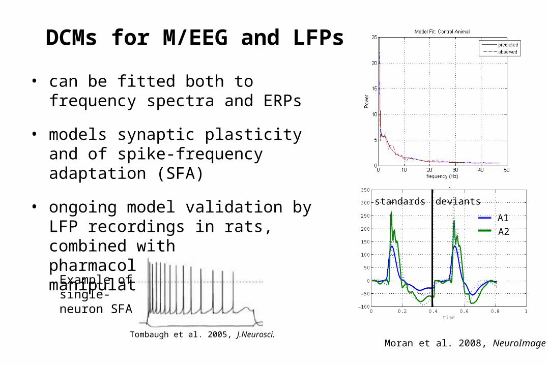
DCMs for M/EEG and LFPs

• can be fitted both to frequency spectra and ERPs

• models synaptic plasticity and of spike-frequency adaptation (SFA)

• ongoing model validation by LFP recordings in rats, combined with pharmacological manipulations

Moran et al. 2008, NeuroImage

standards deviants

A1

A2

Tombaugh et al. 2005, J.Neurosci.

Example of single-neuron SFA

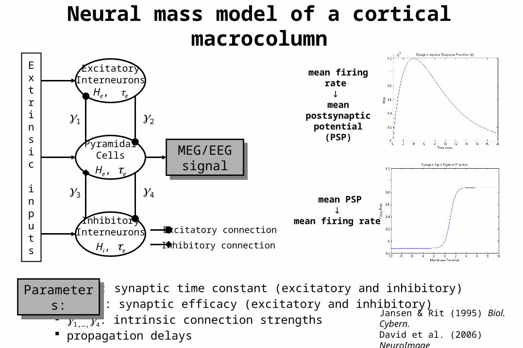
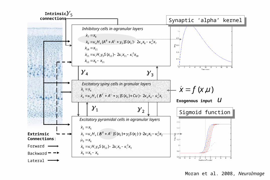
Neural mass model of a cortical macrocolumn

ExcitatoryInterneurons

He, e

PyramidalCells

He, e

InhibitoryInterneurons

Hi, e

Extrinsic inputs

Excitatory connection

Inhibitory connection

e, i : synaptic time constant (excitatory and inhibitory) He, Hi: synaptic efficacy (excitatory and inhibitory) 1,…,: intrinsic connection strengths propagation delays

21

43

MEG/EEGsignal

MEG/EEGsignal

Parameters:

Parameters:

Jansen & Rit (1995) Biol. Cybern.David et al. (2006) NeuroImage

mean firing rate

mean postsynaptic

potential (PSP)

mean PSP

mean firing rate

4 3

1 2

12

4914

41

2))(( xxuaxsHx

xx

eeee

Excitatory spiny cells in granular layers

Exogenous input u

4 3

1 2

Intrinsicconnections

5

Excitatory spiny cells in granular layers

Excitatory pyramidal cells in agranular layers

Inhibitory cells in agranular layers

),( uxfx

11812

102

1112511

1110

72

8938

87

2)(

2)()(

xxx

xxxSHx

xx

xxxSAAHx

xx

iiii

eeLB

ee

12

4914

41

2))()(( xxCuxSAAHx

xx

eeLF

ee

Synaptic ‘alpha’ kernelSynaptic ‘alpha’ kernel

Sigmoid functionSigmoid function

659

32

61246

63

22

51295

52

2)(

2))()()((

xxx

xxxSHx

x

xxxSxSAAHx

xx

iiii

eeLB

ee

Extrinsic

Connections:

Forward

Backward

Lateral

Moran et al. 2008, NeuroImage

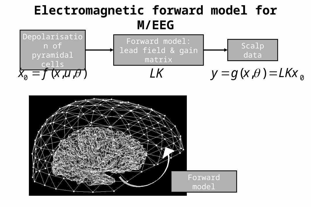
Electromagnetic forward model for M/EEG

Depolarisation of

pyramidal cells

Forward model:lead field & gain

matrixScalp data

),,(0 uxfx LK 0),( LKxxgy

Forward model

Thank you

Documents

DCM: Advanced issues Klaas Enno Stephan Laboratory for Social & Neural Systems Research Institute for Empirical Research in Economics University of Zurich