Embed Size (px)
Citation preview

DC upset resistance weldingModelling and control of a weld
process
G.J.L. Naus
DCT Report no: 2005.8427th of June, 2005
TU/e Master Thesis2004-2005
Supervisors:prof. dr. ir. M. Steinbuch (TU/e)dr. ir. W.J.A.E.M. Post (TU/e)ir. R. Meulenberg (Fontijne Grotnes B.V.)
Engineering thesis committee:prof. dr. ir. M. Steinbuch (Chairman, TU/e)dr. ir. W.J.A.E.M. Post (TU/e)ir. P.C. Teerhuis (TUD)dr. ir. R.H.B. Fey (TU/e)ir. R. Meulenberg (Advisor, Fontijne Grotnes B.V.)
University of Technology Eindhoven (TU/e) Fontijne Grotnes B.V.Department of Mechanical Engineering Research and Development groupDivision Dynamical Systems DesignControl System Technology group

2

Abstract
Fontijne Grotnes B.V. produces wheel rim production lines for the automotive industry. The DCupset resistance weld process is part of these lines. Coiled sheets are welded to a cylinder, whichare used as basis for the final wheel rims. The control and the present theoretical basis of thisweld process are mainly based on practical experience. It is difficult to define the quality of aweld with respect to the weld process or to influence the quality of a weld. Temperature progressduring the weld process is not defined nor measured and the position is not actively controlledalthough these are the most important variables of the weld process.
Consequently a theory, based on the equilibria present in the systems of the weld process, isdeveloped. Experiments are performed to validate this theory. The various parts of the weld pro-cess are modelled and combined to a simulation model for off-line simulation of the process. Thismodel is validated by comparing the resulting pressure, electrical current and position progressto experimental results. Special attention is given to the modelling and control of the hydraulicsystem. This has resulted in a relatively easy model-based controller design and a paper on themodelling and control of hydraulic systems focussing on position control.
Based on the renewed and extended insight in the weld process, a new control strategy has beendeveloped. A MIMO feedback tracking controller is developed based on an on-line temperaturecalculation using classic control actions. The temperature, pressure and position progress duringthe weld process now are user-defined by means of reference trajectories. To facilitate workingwith the MIMO control problem, MCDesign, a tool for MIMO controller design is developed. Thenew control strategy is implemented and tested successfully.
i

ii ABSTRACT
Samenvatting
Fontijne Grotnes B.V. produceert productie straten voor de fabricage van velgen. Het gelijkstroomweerstand stuik lasproces is onderdeel van deze straten. Rond gebogen metalen platen worden totcylinders gelast. Deze cylinders vormen de basis voor de uiteindelijke velg. De beheersing van hetlasproces en de huidige theoretische basis hiervan, zijn voornamelijk op trial and error gebaseerd.Het is lastig om de kwaliteit van een las te benvloeden en deze te relateren aan het lasproces.De proces temperatuur en het verloop van de positie zijn de belangrijkste proces variabelen. Deproces temperatuur is echter niet gedefinieerd en wordt ook niet gemeten. Daarnaast wordt depositie niet actief geregeld.
Daarom is een theorie ontwikkeld die gebaseerd is op de evenwichten van de in het lasprocesaanwezige systemen. Experimenten zijn uitgevoerd om deze theorie te onderbouwen. De verschil-lende onderdelen van het lasproces zijn gemodelleerd en gecombineerd tot een simulatiemodel,waarmee het proces off-line gesimuleerd kan worden. Het model is gevalideerd door het verloopvan de druk, de elektrische stroom en de positie te vergelijken met experimentele resultaten. Demodellering en regeling van het hydraulische systeem hebben speciale aandacht gekregen. Ditheeft geresulteerd in een relatief eenvoudig model-gebaseerd ontwerp van een regeling. Daarnaastis een paper geschreven over het modelleren en regelen van een hydraulisch systeem, waarbij defocus ligt op positie regeling.
Een nieuwe regelstrategie is ontwikkeld op basis van het vernieuwde en uitgebreide inzicht inhet lasproces. Gebaseerd op een on-line temperatuur berekening is een MIMO feedback regelaarontworpen, waarbij gebruik is gemaakt van klassieke regeltechniek. Het verloop van de tem-peratuur, de druk en de positie tijdens het lasproces wordt nu voorgeschreven door middel vanreferentie trajectories. Om het ontwerp van MIMO regelaars te vergemakkelijken, is MCDesignontwikkeld. De nieuwe regel strategie is gemplementeerd en succesvol getest.
iii

iv SAMENVATTING

Contents
Abstract i
Samenvatting iii
Nomenclature and parameters vii
Preface xi
1 Introduction 11.1 Fontijne Grotnes B.V. . . . . . . . . . . . . . . . . . . . . . . . . . . . . . . . . . . 11.2 A rim production line . . . . . . . . . . . . . . . . . . . . . . . . . . . . . . . . . . 11.3 Assignment . . . . . . . . . . . . . . . . . . . . . . . . . . . . . . . . . . . . . . . . 3
2 The weld process 52.1 Experimental setup . . . . . . . . . . . . . . . . . . . . . . . . . . . . . . . . . . . . 52.2 DC upset resistance welding . . . . . . . . . . . . . . . . . . . . . . . . . . . . . . . 5
2.2.1 Gap-closing . . . . . . . . . . . . . . . . . . . . . . . . . . . . . . . . . . . . 72.2.2 Heating . . . . . . . . . . . . . . . . . . . . . . . . . . . . . . . . . . . . . . 92.2.3 Yielding . . . . . . . . . . . . . . . . . . . . . . . . . . . . . . . . . . . . . . 102.2.4 Curing . . . . . . . . . . . . . . . . . . . . . . . . . . . . . . . . . . . . . . . 102.2.5 Exit phase . . . . . . . . . . . . . . . . . . . . . . . . . . . . . . . . . . . . . 11
2.3 Experiments . . . . . . . . . . . . . . . . . . . . . . . . . . . . . . . . . . . . . . . . 112.3.1 Stiffness and damping of the material . . . . . . . . . . . . . . . . . . . . . 122.3.2 Mechanics: slip and initial gap . . . . . . . . . . . . . . . . . . . . . . . . . 152.3.3 Switching between the phases . . . . . . . . . . . . . . . . . . . . . . . . . . 162.3.4 Contact and bulk resistance . . . . . . . . . . . . . . . . . . . . . . . . . . . 182.3.5 Time of the weld process . . . . . . . . . . . . . . . . . . . . . . . . . . . . 21
3 Modelling 253.1 Introduction . . . . . . . . . . . . . . . . . . . . . . . . . . . . . . . . . . . . . . . . 25
3.1.1 Previous modelling . . . . . . . . . . . . . . . . . . . . . . . . . . . . . . . . 253.1.2 Goals of modelling . . . . . . . . . . . . . . . . . . . . . . . . . . . . . . . . 263.1.3 Model layout . . . . . . . . . . . . . . . . . . . . . . . . . . . . . . . . . . . 26
3.2 Weld program (WELD2001) . . . . . . . . . . . . . . . . . . . . . . . . . . . . . . . 263.3 Thermodynamics of the weld process . . . . . . . . . . . . . . . . . . . . . . . . . . 27
3.3.1 Discretisation of the working area . . . . . . . . . . . . . . . . . . . . . . . 283.3.2 Heat generation . . . . . . . . . . . . . . . . . . . . . . . . . . . . . . . . . . 293.3.3 Conduction, radiation, convection . . . . . . . . . . . . . . . . . . . . . . . 293.3.4 Internal energy . . . . . . . . . . . . . . . . . . . . . . . . . . . . . . . . . . 303.3.5 Balances of energy . . . . . . . . . . . . . . . . . . . . . . . . . . . . . . . . 31
3.4 Mechanics of the weld process . . . . . . . . . . . . . . . . . . . . . . . . . . . . . . 323.4.1 Welding machine . . . . . . . . . . . . . . . . . . . . . . . . . . . . . . . . . 323.4.2 Mechanical behaviour of the material . . . . . . . . . . . . . . . . . . . . . 33
v
vi CONTENTS
3.5 Converter system . . . . . . . . . . . . . . . . . . . . . . . . . . . . . . . . . . . . . 343.6 Hydraulic system . . . . . . . . . . . . . . . . . . . . . . . . . . . . . . . . . . . . . 35
3.6.1 Overview of the hydraulic system . . . . . . . . . . . . . . . . . . . . . . . . 363.6.2 White box modelling . . . . . . . . . . . . . . . . . . . . . . . . . . . . . . . 363.6.3 Measurements and black box modelling . . . . . . . . . . . . . . . . . . . . 383.6.4 Control of the hydraulic system . . . . . . . . . . . . . . . . . . . . . . . . . 38
3.7 Modelling results . . . . . . . . . . . . . . . . . . . . . . . . . . . . . . . . . . . . . 39
4 Control 434.1 Demands to the controller . . . . . . . . . . . . . . . . . . . . . . . . . . . . . . . . 434.2 Control strategy . . . . . . . . . . . . . . . . . . . . . . . . . . . . . . . . . . . . . 444.3 Temperature calculation and simplified model . . . . . . . . . . . . . . . . . . . . . 454.4 Linearisation . . . . . . . . . . . . . . . . . . . . . . . . . . . . . . . . . . . . . . . 47
4.4.1 Theory . . . . . . . . . . . . . . . . . . . . . . . . . . . . . . . . . . . . . . 474.4.2 Implementation . . . . . . . . . . . . . . . . . . . . . . . . . . . . . . . . . . 484.4.3 Results . . . . . . . . . . . . . . . . . . . . . . . . . . . . . . . . . . . . . . 49
4.5 Reference trajectories . . . . . . . . . . . . . . . . . . . . . . . . . . . . . . . . . . 504.5.1 Design of the reference trajectories . . . . . . . . . . . . . . . . . . . . . . . 504.5.2 Material determination . . . . . . . . . . . . . . . . . . . . . . . . . . . . . 52
4.6 Controller design . . . . . . . . . . . . . . . . . . . . . . . . . . . . . . . . . . . . . 524.6.1 Sequential loop closing . . . . . . . . . . . . . . . . . . . . . . . . . . . . . . 534.6.2 Loop shaping . . . . . . . . . . . . . . . . . . . . . . . . . . . . . . . . . . . 554.6.3 Switching control . . . . . . . . . . . . . . . . . . . . . . . . . . . . . . . . . 584.6.4 Learning control . . . . . . . . . . . . . . . . . . . . . . . . . . . . . . . . . 59
4.7 Implementation and results . . . . . . . . . . . . . . . . . . . . . . . . . . . . . . . 61
5 Conclusions and recommendations 65
6 References 69
A FRW-series welding machine 73
B Simulation models and URW Library 75
C Modelling of the hydraulic system 77C.1 White box modelling . . . . . . . . . . . . . . . . . . . . . . . . . . . . . . . . . . . 77
C.1.1 Electric hydraulic servo valve . . . . . . . . . . . . . . . . . . . . . . . . . . 77C.1.2 Hydraulic cylinder . . . . . . . . . . . . . . . . . . . . . . . . . . . . . . . . 80C.1.3 External mechanics . . . . . . . . . . . . . . . . . . . . . . . . . . . . . . . . 83
C.2 Measurements . . . . . . . . . . . . . . . . . . . . . . . . . . . . . . . . . . . . . . . 84C.3 Black box modelling . . . . . . . . . . . . . . . . . . . . . . . . . . . . . . . . . . . 86
D Weld process model 89D.1 Nonlinear state-space model . . . . . . . . . . . . . . . . . . . . . . . . . . . . . . . 89D.2 Transfer functions . . . . . . . . . . . . . . . . . . . . . . . . . . . . . . . . . . . . 91
E MCDesign 95
F Matlab tools 97

Nomenclature and parameters
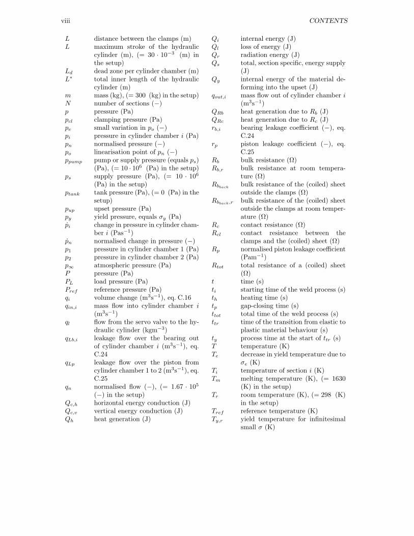
The parameters defined in this list of nomenclature correspond to the setup at Fontijne GrotnesB.V. and the material used in the experiments described in section 2.3.
ao radius of a circle (m), eq. 2.14A cross section of a (coiled) sheet
(mm2)Ac contact surface between the sheet
ends (m2)Aeff effective cylinder surface (m2), (=
1.57 · 10−3 (m2) in the setup)Ap cross section surface of the piston
(m2), (= 2.8 · 10−3 (m2) in thesetup)
Ar cross section surface of the rod (m2),(= 1.3 · 10−3 (m2) in the setup)
b diameter of the orifice of the spoolvalve (m), eq. C.4
cd compensation factor (kg−0.5m1.5),eq. C.4
Co hydraulic stiffness (Pam)Cp specific heat (Jkg−1K−1)d damping (Nsm−1)del elastic damping of the material
(Nsm−1), (= 5.0 · 106 (Nsm−1) inthe setup)
dm damping of the material (Nsm−1)dp piston diameter (m), (= 65 · 10−3
(m) in the setup)dpl plastic damping of the material
(Nsm−1)dpr rod diameter (m), (= 40 · 10−3 (m)
in the setup)dx part of L (m), eq. 3.1dx speed of displacement (ms−1)dV volume (m3)dy (a part of the) width of a (coiled)
sheet (m)
dz (a part of the) height of a (coiled)sheet (m)
E Young’s modulus (Pa)Eoil oil stiffness (Pa), (= 8 · 108 (Pa) in
the setup)F force (N)Ff friction force (N)Fup upset force (N)G approximation gain (−), (= 1 · 106
(−) in the setup), eq. C.14GFf 1 friction force gain (−), (= 7.63 · 105
(−) in the setup), eq. 3.15GFf 2 average friction force (−), (= 7.63 ·
105 (−) in the setup), eq. 3.15h height of a (coiled) sheet (m)HB Brinell Hardness (Pa)HBr Brinell Hardness at room tempera-
ture (Pa), (= 200 · 106 (Pa) in thesetup)
i electrical current (A)
i change in electrical current per timeunit (A)
i1 electrical current directed throughthe material in between the clamps(A)
i2 electrical current directed throughthe material outside the clamps (A)
k stiffness(Nm−1)kel elastic stiffness of the material
(Nsm−1), (= 87.5 · 106 (Nsm−1) inthe setup)
km stiffness of the material (Nsm−1)kpl plastic stiffness of the material
(Nsm−1), (= 0 (Nsm−1) in thesetup)
vii
viii CONTENTS
L distance between the clamps (m)L maximum stroke of the hydraulic
cylinder (m), (= 30 · 10−3 (m) inthe setup)
Ld dead zone per cylinder chamber (m)L∗ total inner length of the hydraulic
cylinder (m)m mass (kg), (= 300 (kg) in the setup)N number of sections (−)p pressure (Pa)pcl clamping pressure (Pa)pe small variation in po (−)pi pressure in cylinder chamber i (Pa)pn normalised pressure (−)po linearisation point of pn (−)ppump pump or supply pressure (equals ps)
(Pa), (= 10 · 106 (Pa) in the setup)ps supply pressure (Pa), (= 10 · 106
(Pa) in the setup)ptank tank pressure (Pa), (= 0 (Pa) in the
setup)pup upset pressure (Pa)py yield pressure, equals σy (Pa)pi change in pressure in cylinder cham-
ber i (Pas−1)pn normalised change in pressure (−)p1 pressure in cylinder chamber 1 (Pa)p2 pressure in cylinder chamber 2 (Pa)p∞ atmospheric pressure (Pa)P pressure (Pa)PL load pressure (Pa)Pref reference pressure (Pa)qi volume change (m3s−1), eq. C.16qin,i mass flow into cylinder chamber i
(m3s−1)ql flow from the servo valve to the hy-
draulic cylinder (kgm−3)qLb,i leakage flow over the bearing out
of cylinder chamber i (m3s−1), eq.C.24
qLp leakage flow over the piston fromcylinder chamber 1 to 2 (m3s−1), eq.C.25
qn normalised flow (−), (= 1.67 · 105
(−) in the setup)Qc,h horizontal energy conduction (J)Qc,v vertical energy conduction (J)Qh heat generation (J)
Qi internal energy (J)Ql loss of energy (J)Qr radiation energy (J)Qs total, section specific, energy supply
(J)Qy internal energy of the material de-
forming into the upset (J)qout,i mass flow out of cylinder chamber i
(m3s−1)QRb heat generation due to Rb (J)QRc heat generation due to Rc (J)rb,i bearing leakage coefficient (−), eq.
C.24rp piston leakage coefficient (−), eq.
C.25Rb bulk resistance (Ω)Rb,r bulk resistance at room tempera-
ture (Ω)Rbback
bulk resistance of the (coiled) sheetoutside the clamps (Ω)
Rbback,r bulk resistance of the (coiled) sheetoutside the clamps at room temper-ature (Ω)
Rc contact resistance (Ω)Rcl contact resistance between the
clamps and the (coiled) sheet (Ω)Rp normalised piston leakage coefficient
(Pam−1)Rtot total resistance of a (coiled) sheet
(Ω)t time (s)ti starting time of the weld process (s)th heating time (s)tp gap-closing time (s)ttot total time of the weld process (s)ttr time of the transition from elastic to
plastic material behaviour (s)ty process time at the start of ttr (s)T temperature (K)Te decrease in yield temperature due to
σe (K)Ti temperature of section i (K)Tm melting temperature (K), (= 1630
(K) in the setup)Tr room temperature (K), (= 298 (K)
in the setup)Tref reference temperature (K)Ty,r yield temperature for infinitesimal
small σ (K)
CONTENTS ix
Tcd speed of cooling down (Ks−1)ui inverter control signal (mA), (=
0 . . . 1 (mA) in the setup)uv servo valve control signal (mA), (=
−1 . . . 1 (mA) in the setup)U potential difference over the clamps
(V)v speed (ms−1)V volume (m3)Vi volume of cylinder chamber i (m3)
Vi volume change of cylinder chamberi (m3s−1)
w width of a (coiled) sheet (m)x distance between the clamps (m)x length of the orifice of the spool
valve(m), eq. C.4xe small variation in xo (−)xin displacement of the spool valve (m)xmax maximum stroke of the spool valve
(m)xn normalised spool valve displacement
(−)xo linearisation point of xn (−)xout displacement of the spool valve (m)x speed of displacement of the right
clamp (ms−1)xn velocity of the normalised spool
valve displacement (−)x acceleration (ms−2)y displacement of the rod (m)yref reference position (m)y speed of the rod (ms−1)
Greek letters
αth thermal expansion coefficient (K−1)αrho coefficient of thermal resistance
(ΩmK−1)∆P pressure difference (Pa)∆T difference in temperature (K)∆v difference in speed (ms−1)∆σ difference in stress (Pa)ε strain (m)ε overlap of the servo valve (m), (= 0
(m) in the setup), eq. C.7εP pressure error (Pa)εth emissivity constant (m), (= 0.56
(m) in the setup)
εT temperature error (K)εy yield strain (m)εy position error (m)η linearisation point of xn (−)λ coefficient of thermal conductivity
(Jm−1K−1)ξcs damping of ωcs (−), (= 0.6 (−) in
the setup)ξv damping of ωv,o (−), (= 0.7 (−) in
the setup)ξURW compensation factor (−), (= 12 (−)
in the setup), eq. 2.20ξZm compensation factor (−), (= 3 (−)
in the setup), eq. 2.16ρ specific mass (kgm−3), (= 7850
(kgm−3) in the setup)ρi oil density of cylinder chamber i
(kgm−3)ρe electrical resistivity (Ωm)ρo oil density at atmospheric pressure
(kgm−3)ρe,r electrical resistivity at room tem-
perature (Ωm), (= 3.45 ·10−4 (Ωm)in the setup)
ρ change in oil density (kgm−3s−1)σ stress (Pa)σe external stress (Pa)σy yield stress (Pa)σy,I−II yield stress at the switch from phase
I to II (Pa)σy,II−III yield stress at the switch from phase
II to III (Pa)σy,r yield stress at room temperature
(Pa)Φi mass flow of cylinder chamber i
(kgs−1)ωcs natural frequency of the converter
system (Hz), (= 1000 (Hz) in thesetup)
ωo natural frequency of the hydrauliccylinder (Hz)
ωv,o natural frequency of the servo valve(Hz), (= 200 (Hz) in the setup)

x CONTENTS

Preface
The assignment discussed in this report was executed at Fontijne Grotnes B.V. in Vlaardingen,within the framework of a Master’s Thesis at the department of mechanical engineering of Eind-hoven University of Technology. The assignment is a result of the R&D-team of Fontijne GrotnesB.V. examining the DC upset resistance weld process used in their wheel rim production lines.Accordingly, the assignment was performed working in this team.
The weld process involved is driven by a force and an electrical current. The process is dividedinto 5 phases based on position and time restrictions. The current weld program prescribes aconstant force and electrical current in each phase, depending on the measured position andtime. Based on understanding the process, a new control strategy has to be developed includingcontinuous control of significant process variables. The original assignment consisted of threeparts. The first part was to expand and create a better insight in the weld process, secondly todevelop a reliable model of the process to contribute to this insight and finally to develop a newcontrol strategy.
In the first chapter an introduction of the weld process used is given and the assignment isexpound and defined. A description of the weld process, including a theoretical approach and anexperimental validation is discussed in Chapter 2. In the next chapter a model of the weld processand the various systems is developed, from which a simulation model results. Special attentionis paid to the modelling and control of the hydraulic system. In Chapter 4 the development ofa new control strategy including the implementation and the results, is discussed. To facilitatethe design of the controller, a tool specialised in dealing with MIMO control problems has beendeveloped.
Besides the stated assignment, the goal was to become familiar with working in a medium-sizedcompany like Fontijne Grotnes B.V. A nice cooperation with the other members of the team andfellow students at the company were instructive and pleasant. Furthermore, the experience of ayear working at the company and going through the various departments and projects gave a goodimpression of the company.
xi

xii PREFACE
Chapter 1
Introduction
1.1 Fontijne Grotnes B.V.
Fontijne Grotnes B.V. [Fontijne, (web)] was established in 2000 by the acquisition of GrotnesMetalforming Systems, Chicago, Illinois, U.S.A., by Fontijne Holland, Vlaardingen, the Nether-lands. A company combining nearly 200 years of experience as a manufacturer of metalformingequipment for the wheel industry, sizing equipment, nuclear supercompactors, laboratory platenpresses and services was established. Fontijne is a leading European supplier of wheel and rimmanufacturing systems, while Grotnes continues to supply other markets, with the two companiesworking in co-operation to innovate the product line and lead the industry.
Figure 1.1: the company logo of Fontijne Grotnes B.V.
Fontijne develops custom machinery solutions for the expanding, coiling, rotary roll formingand welding of cylindrical metal parts. These parts are utilised in transportation, aerospace,agriculture, petroleum, appliance, and forging industries. Their customers’ products range fromthe simple: wheel rims and pipe couplings, to the sophisticated: missile tubes and jet engine ringsand nozzles. Fontijne can carry out an entire forming process or a single production module.
1.2 A rim production line
The wheel rim production lines developed by Fontijne vary in the range of very small spare tirerims for passenger cars to large rims for industrial trucks. So cross section of about 350 mm2 to3000 mm2 and more are involved. Fontijne produces completely automated and hand supportedproduction lines as well as parts of the lines and single machines. Several techniques to producerims exist like deep drawing and casting (for example for aluminum rims). At Fontijne, however,the rims are made out of a sheet of metal which is coiled, welded and profiled. A production line forthis kind of process consists of five main parts, each including various fabrication / production stepsand separate machines. In Figure 1.2 an overview of the processes in a complete rim productionline is shown.
The rim production line starts with a straightener. The straightener uncoils and cuts thematerial, which is supplied on big coils. In the preparation line, the cut-to-length sheets are coiledand welded to cylinders. This line ends with the removal of the upset resulting from the welding.
1

2 CHAPTER 1. INTRODUCTION
profilingwelding
coiling
welddressing
valve hole punching
leak detecting
4 torch welding
assembly pressing
cutting
uncoiling
expanding
flaring
preparationline
profilingline
cut-to-lengthline
assemblyline
painting
painting
Figure 1.2: overview of the processes in a rim production line.
Next the profile is formed into the rims. Most loss of rims occurs at the flaring process due tocracking at the welding seams or just beside it. In this flaring process two cones are pressed intoboth sides of the cylinders. The profiling ends with an expanding step to give the rims their finalsize. The total production line ends with painting, after a leak detection test, the punching of avalve hole and the assembly of a disc into the rims.
The machinery for the rim production line is partly developed by Fontijne itself and partlyacquired. One of the machines that Fontijne has developed itself is the direct current (DC) upsetresistance welding machine [Fontijne, 2001]. The involved weld process is a butt welding processused in rim production lines and for example spot welding. Two sheet of metal are pushed togethersideways with a large amount of force. An electrical current is directed through the sheets andheat is formed due to the resistance to conduct electrical current of the butt-joined material. Thisresistance is highest at the seam between the two sheets. When the temperature is high enough, thesheet ends start to yield, upset is formed and the sheets are welded together [key-to-steel, (web)].Commonly used for this kind of weld process are alternating current (AC) welders because of theirrobustness. Using AC welding, the temperature is increased to the metal’s melting temperature.An arc arises over the seam between the two sheets and the melting metal spatters away. In thisway the usually polluted sheet ends are burned away. If enough of the metal is burned away, thesheets are welded together. This costs a lot of energy and requires much power, not only becausethe metal is burned away, but also by the use of alternating current. Using alternating currentinstead of direct current, the peak currents needed to achieve a certain average (RMS), are muchhigher. This affects the efficiency of the energy transfer to the welding seam and makes the processmore susceptible to abortion. Using DC welding, the metal is only heated to its yield temperatureand then welded together. In this way the weld process elapses much smoother and accordinglycan be controlled more easily. Shorter weld times, less energy consumption, less loss of materialand no spattering, which makes it a much cleaner process, are the main advantages [Kucklick,1996].
The quality of a weld is defined to be good if the weld survives the imposed deformations
1.3. ASSIGNMENT 3
of the following processes in the rim production line. The flaring process is the first significantdeformation step after the weld process. At this process up to 2% loss of rims is present dueto cracking at the welding seam or just beside it. The quality of the weld is dependent on thetemperature progress of the material during the weld process [Mast, 2000], [Put,1999], [NIMR,2005]. The NIMR (Netherlands Institute for Metal Research) [NIMR, (web)] is doing research inthis field, which has to result in guidelines for an optimal progress of the weld process. In thisway the quality of a weld can be determined from the results of the weld process itself and besidesmay be influenced willfully.
Fontijne has developed their own welding machine series for the DC upset resistance weldprocess, the Fontijne Resistance Welders (FRW-series) [Fontijne, 2001]. An overview of the weldprocess and the welding machine used is given in Chapter 2. The software to control the process,WELD2000 [Fontijne, 2000], is developed by Fontijne itself as well. It is implemented on theFRW-series. Nowadays Fontijne is making a new move by implementing WELD2000 at weldingmachines of competitors already in the field. Supported by the success of this strategy, control ofthe weld process has become one of the points of attention of the company. Customers are veryinterested in new developments in this field since problems exist with current rim production linesthat are attributed to the weld process. If the weld process becomes more robust and reliable,not only failure can be diminished, but it also gives sight at shorter welding times. The weldprocess often is one of the bottleneck processes as for time consuming processes in a automatedrim production line. So the benefit of a tenth of a second per produced rim pays off a lot inproducing 900 to 1100 rims per hour.
Consequently this study to the DC upset resistance weld process as performed at Fontijne,first of all is aimed at a good insight in the process. This has to result in a more robust andreliable control strategy. Besides, if the process is more robust and reliable, other advantages maybe taken advantage of like decrease of the needed upset. At the moment, simply a large upset isused to be sure all the pollution in the welding seam is removed and the resulting weld is airtight.The amount of energy used may be optimised by which energy can be saved. Furthermore theinsight in the process may be expanded to other resistance welding principles like spot welding.
1.3 Assignment
The assignment as initially defined by Fontijne consisted of two main parts. Firstly the alreadyavailable theory and modelling of the DC upset resistance weld process had to be completed.Secondly a new controller for the weld process had to be developed, based on the attained insightin the weld process. The controller would be position or pressure based and eventually parts ofthe controller might become learning because of the repetitive character of the process.
The available theory and modelling appeared to be too fragmented to simply complete anduse as a base for the development of a controller. Consequently the insight in the weld processand modelling part of the assignment are emphasised in the first place. The feasibility of thedevelopment of a test setup containing a hydraulic system and nonlinear springs was examined.This was stopped when the damping instead of the stiffness of the material appeared to be mostsignificant in the second part of the process. A simulation model to perform off-line simulationsof the weld process has to be developed to contribute to the validity of the resulting theory andmodelling. Next the MIMO control problem has to be solved in a way the resulting controlleris based on the theory and modelling. In designing the controller the complexity of it has to betaken into account considering implementation of it at welding machines in the field.
A secondary requirement of the assignment was a structured and well documented way ofworking so that others are able to use the developed tools and performed experiments as well.

4 CHAPTER 1. INTRODUCTION

Chapter 2
The weld process
Before modelling can take place, a good insight in the weld process is inevitable and needed. Vari-ous studies to the weld process are performed already. The most significant studies are Meulenberg[2002], Put [1999] and Legemaate [1997]. In most cases however, only a short overview of the weldprocess is used as a direct introduction to modelling. Up till now, a lack of insight in the processhas resulted in problems further on in the development of a new control strategy. Consequentlythis study is started with an overview of the systems and the equilibria present during the weldprocess. This is followed by a discussion of the results of experiments. These experiments areperformed to contribute to the insight in the process and validate the theory. To start with, theexperimental setup used during this study is discussed and an introduction to the weld process isgiven.
2.1 Experimental setup
The FRW-series are the welding machines produced and developed by Fontijne [Fontijne, 2001](see Appendix A). They contain some disadvantages as follows from Appendix A. Their operationmay be improved by a redesign of the machine as well as the control strategy. Consequently theexperimental setup used in this study was developed [Louter, 1999], [Ledeuil 1998], [Allersma,1999]. It is called the Fontijne Holland Welder (FHW). The setup is a first model for a possiblesuccessor of the FRW-series and has to facilitate the study to this redesign.
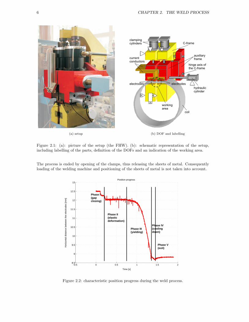
In Figure 2.1(a) a picture of the setup is shown. In Figure 2.1(b) a schematic overview of thesetup including an indication of the degrees of freedom (DOF) of the structure of the setup, isgiven. The setup is smaller than the FRW-series, so its weld capacity is limited. Hence two smallersheets instead of a coiled sheet are used in the welding process. Only one clamping mechanism canmove in horizontal direction (see Figure 2.1(b)). The position of the clamping mechanisms is stilldetermined by measuring the displacement of the rod. In this case however, the rod is mountedin line with the clamping mechanisms. Moreover, the movement of the clamping mechanismsis a linear motion instead of a rotation. The pressure difference across the hydraulic cylinderis measured as well. Besides that, the potential over the clamps and the electrical current aremeasured. The total setup is controlled by a digital dSpace system. This system combines aSimulink model, Controldesk and the data acquisition of the machine to control the weld process.A complete overview of the working of the upset resistance weld process performed on this setup,is given in the next sections.
2.2 DC upset resistance welding
The DC upset resistance weld process is part of the rim production line (see section 1.2). Thepurpose of the process is to close a coiled sheet of metal by welding the sheet ends together. Inthe scope of this study, the start of the process is limited to clamping of the sheets of metal.
5
6 CHAPTER 2. THE WELD PROCESS
(a) setup
hydrauliccylinder
coil
electrodes
currentconductors
C-frame
hinge axis ofthe C-frame
clampingcylinders
workingarea
electrodes
auxiliaryframe
(b) DOF and labelling
Figure 2.1: (a): picture of the setup (the FHW). (b): schematic representation of the setup,including labelling of the parts, definition of the DOFs and an indication of the working area.
The process is ended by opening of the clamps, thus releasing the sheets of metal. Consequentlyloading of the welding machine and positioning of the sheets of metal is not taken into account.
−0.5 0 0.5 1 1.5 28.5
9
9.5
10
10.5
11
11.5
12
12.5
13
Time [s]
Hor
izon
tal d
ista
nce
betw
een
the
elec
trod
es [m
m]
Position progress
Phase I (gap closing)
Phase II (elastic deformation)
Phase III (yielding)
Phase IV(coolingdown)
Phase V(exit)
Figure 2.2: characteristic position progress during the weld process.

2.2. DC UPSET RESISTANCE WELDING 7
Till now, the DC upset resistance weld process has been divided into 5 sequential phases. Thisdivision is based on the distance between the clamps or electrodes (see also section 3.2). Thedistance between the electrodes is determined on-line. The weld program uses this distance tosteer the electrical current and force, needed in the weld process. A characteristic progress ofthe displacement during the weld process is depicted in Figure 2.2. First the welding machine isloaded and the coiled sheet is clamped. Secondly the coil ends are pushed together to close theinitial gap in between them. Next the material is heated. If it reaches its yield temperature, theactual welding (or yielding) takes place. The amount of displacement determines when a weld isformed. The electrical current is switched off. After a curing time in which the weld cools downand hardens, the pressure is released. Finally the welded coil is removed from the machine.
In developing a theory for the weld process, the emphasis lies on a small part of the weldingmachine. This so-called working area is shown in Figure 2.3 and also indicated in Figure 2.1(b).The working area involves the metal sheets that are welded together and the electrodes clampingthe material.
weldingseam
rightclampingelectrode
left clampingelectrode
sheetof metal
Figure 2.3: close up of the working area of the setup (see also Figure 2.1(b)): the electrodes andthe two sheets of metal. In the right figure the degrees of freedom (DOF) of the electrodes areindicated.
The present weld philosophy is based on a division of the weld process into 5 phases. Ac-cordingly, the examination of the weld process is divided into 5 parts as well. The systems andequilibria present in each of these 5 phases are discussed in this section. First a short introductionper phase is given. After that, each phase is discussed point to point and the most importantvariables are explained in more detail. In this way a theory describing the DC upset resistanceweld process is developed. This theory is verified by means of experiments and simulations (seesection 2.3 and Chapter 3).
2.2.1 Gap-closing
First the sheets of metal are clamped by two independent clamps. Next the sheet ends are pushedtogether with a predefined force. This force is applied by means of a hydraulic cylinder mountedto the right clamp, see Figure 2.8. This clamp is the only one with a degree of freedom (DOF)in horizontal direction. The inital gap between the sheet ends is eliminated and a contact surfacebetween the two ends, the welding seam, is created. Loading coiled sheets, in practice also aso-called slip-control is present. Slip-control involves compensation for misalignment of the sheetends (as far as this is possible). This misalignment originates from the coiler. The coiler can notadept to varying internal stresses in the material, which results in coiled sheets with a varying

8 CHAPTER 2. THE WELD PROCESS
initial gap. Using the setup instead of the FRW-series two separate sheets are used and thus noslip-control is needed.
Pcl Pcl
Fup
x=initial gap
welding seam
right clamp
left clamp
sheetof metal
Figure 2.4: phase I: gap-closing
• The sheets are clamped with a predefined clamping pressure pcl of 9 · 106 to 10 · 106 Pa.
• The sheet ends are pushed together with a constant upset force Fup. This force is appliedat one side by means of a hydraulic cylinder.
• Fup is proportional to the pressure of the hydraulic system pL: pL = Fup/Acyl, with Acyl
the effective cylinder surface.
• The sheets are initially cut-to-length, which results in a certain surface coarseness of thesheet ends. Due to this coarseness, contact points are formed between the sheet ends bymeans of the upset force. The total surface of the contact points is summed to a contactsurface Ac between the sheet ends. This contact surface is smaller than the cross section ofthe material.
• The pressure on the contact surface, pup, is proportionally to the size of the surface: pup =Fup/Ac, so pup = pup(Ac). During the setup of the upset force, the pressure on the contactsurface will increase till the yield stress of the material. If it equals the yield stress thedeformation of the contact points will become plastic. Till then, elastic deformation ofthe contact points is present. In this way the cross section of the contact points enlarges.Besides that, the gap between the sheet ends decreases and new contact points are formed.So the size of the total contact suface Ac increases. The deformation of the contact pointsis catalysed by the upset pressure pup > σy and will stop when the upset pressure equalsthe yield stress: pup = σy(ε, T, σy,o). The force due to elastic deformation of the materialpresent in the welding seam, now equals the upset force. To describe this process, the nextassumptions are made:
– The temperature change as a result of the deformation is negligible and is thereforeassumed to be constant.
– After the elastic deformation of the first contact points, the deformation becomesplastic. Because the temperature is taken constant, this is cold deformation. Hencestrengthening is present. However, the contact surface Ac increases by means of thisplastic deformation. This results again in elastic deformation of material. Consequentlyas long as the contact surface grows, the deformation can be seen as elastic. The effectof strengthening, σy(ε) = σy, which is a result of plastic deformation, thus is neglected.
So now σy(ε, T, σy,o) = σy,o holds, with σy,o the yield stress of the material at room temper-ature.
• Phase II starts after an at beforehand given displacement x or time, see section 3.2. Thesebounds to the displacement and the time are determined by trial and error and normallyare about 1.0 mm respectively 0.2 s.

2.2. DC UPSET RESISTANCE WELDING 9
The result is an equilibrium between the contact surface Ac, the upset pressure pup and theupset force Fup. With the upset pressure pup equal to the yield stress σy = σy,o = σy,I−II and ata temperature T = Tr.
2.2.2 Heating
When the gap between the sheet ends is closed, an electrical current is switched on over theresulting welding seam. This electrical current is applied using the clamps, with which the coil isclamped, as electrodes. Because of the contact surface between the sheet ends is smaller than thecross section of the sheets, a restriction resistance exists. In literature this is called the contactresistance Rc, which will be used further on. Besides that, the electrical resistance of the material,called the bulk resistance, is present. Combination of the electrical current and these resistancesresult in heat generation.
Pcl Pcl
Fup
x=xel
i
Figure 2.5: phase II: heating
• Apart from the present upset force Fup, a constant electrical current i is applied at thewelding seam.
• A contact resistance Rc and the bulk resistance Rb of the material are present.
• Combination of the electrical current and the present resistances result in heat generationQh = i(Rc + Rb). The total resistance is largest at the welding seam. Consequently heatgeneration starts at the welding seam. The bulk resistance increases accordingly to thetemerature of the material. Hence it is largest at the welding seam and heat generation alsoproceeds at the welding seam.
• Through for example conduction and radiation, energy Ql will be lost. The material isheated with the resulting energy.
• The contact resistance, as well as the bulk resistance are temperature dependent and increaseat higher temperatures. Besides, Rc is inverted proportional to the contact surface Ac.Consequently it will decrease when Ac increases.
• The yield stress σy decreases when temperature increases. This disrupts the equilibriumσy,I−II = pup, causing the material to deform. This deformation is the same as describedat section 2.2.1. Hence, the upset pressure pup decreases along with the yield stress to keepthe process at equilibrium.
• The contact surface Ac increases by this deformation till it equals the size of the cross sectionof the sheet, Ac = wh.
• When Ac = wh, the contact resistance Rc vanishes. No restriction in the conducting surfaceis present anymore, so also no resistance is present. Because of the from now on constantcontact surface, the upset pressure becomes linear dependent on the upset force.

10 CHAPTER 2. THE WELD PROCESS
• The yield stress at this point equals σy = Fup/Ac. The material starts yielding if pup > σy.
The result is a contact surface Ac = wh, so the contact resistance Rc becomes zero. The yieldstress σy,II−III equals pup = Fup/Ac. The momentary temperature is called the yield temperatureTy,II−III . If this temperature is increased, the material starts yielding.
2.2.3 Yielding
The material next to the welding seam is heated to the same temperature as the material in thewelding seam. An equilibrium is formed between the speed with which the material reaches theequilibrium temperature and the speed of the plastic deformation. This is catalysed by the upsetpressure pup and the electrical current i. This results in yielding, or plastic deformation, forminga weld with upset in the welding seam. By the plastic deformation, the material is pushed out ofthe welding seam by which the upset is formed. In the modelling, the total displacement by whichthe upset is formed, is called upset.
Pcl Pcl
Fup
x=upset
i
upset
Figure 2.6: phase III: yielding
• The upset pressure pup is linear dependent on the upset force Fup) due to the constantcontact surface Ac. Due to forming of upset, the cross section at the welding seam increasessome more. However pup is assumed to be dependent on the smallest cross section in thematerial. This now equals Ac = wh.
• The magnitude of the bulk resistance Rb depends on the height of the yield temperature atthe end of phase II. Depending on the magnitude of Rb and the magnitude of the electricalcurrent, heat generation Q = Rbi−Ql takes place. The speed of the deformation consequentlydepends on the magnitude of the electrical current and the height of the yield temperatureat the end of phase II. Within limits holds that the higher the yield temperature, the largerthe speed of deformation.
• The temperature increases till a stable equilibrium is formed between the amount of energydissipated by the deformation in the welding seam and the amount of energy applied to thesystem (see section 3.3.4).
The yielding phase is restricted by a maximum deformation or displacement, proportional tothe amount of upset. If the amount of upset is reached, the current is switched off.
2.2.4 Curing
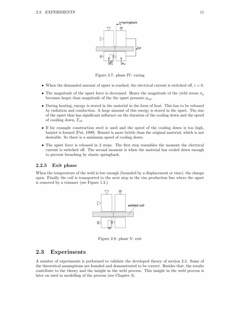
When the demanded amount of upset is reached, the electrical current is switched off. The upsetforce is released stepwise. The first step is to stop the yielding movement but keep pressure onthe newly formed weld so that it can relax. The second step is to prevent a negative force on theweld, which could draw the two sheet ends apart. The material starts cooling down by radiationand mainly conduction.
2.3. EXPERIMENTS 11
Pcl Pcl
Fup
x=springback
Figure 2.7: phase IV: curing
• When the demanded amount of upset is reached, the electrical current is switched off, i = 0.
• The magnitude of the upset force is decreased. Hence the magnitude of the yield stress σy
becomes larger than magnitude of the the upset pressure pup.
• During heating, energy is stored in the material in the form of heat. This has to be releasedby radiation and conduction. A large amount of this energy is stored in the upset. The sizeof the upset thus has significant influence on the duration of the cooling down and the speedof cooiling down, Tcd.
• If for example construction steel is used and the speed of the cooling down is too high,bainiet is formed [Put, 1999]. Bainiet is more brittle than the original material, which is notdesirable. So there is a minimum speed of cooling down.
• The upset force is released in 2 steps. The first step resembles the moment the electricalcurrent is switched off. The second moment is when the material has cooled down enoughto prevent breaching by elastic springback.
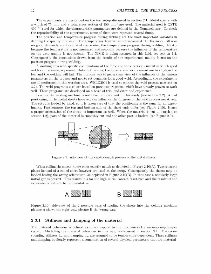
2.2.5 Exit phase
When the temperature of the weld is low enough (bounded by a displacement or time), the clampsopen. Finally the coil is transported to the next step in the rim production line where the upsetis removed by a trimmer (see Figure 1.2.)
welded coil
Figure 2.8: phase V: exit
2.3 Experiments
A number of experiments is performed to validate the developed theory of section 2.2. Some ofthe theoretical assumptions are founded and demonstrated to be correct. Besides that, the resultscontribute to the theory and the insight in the weld process. This insight in the weld process islater on used in modelling of the process (see Chapter 3).
12 CHAPTER 2. THE WELD PROCESS
The experiments are performed on the test setup discussed in section 2.1. Metal sheets witha width of 75 mm and a total cross section of 150 mm2 are used. The material used is QSTE460TM steel for which the characteristic parameters are defined in the Nomenclature. To checkthe reproducibility of the experiments, some of them were repeated several times.
The position and temperature progress during welding are the most important variables indefining the quality of a weld. The temperature however is not measured. Furthermore, till nowno good demands are formulated concerning the temperature progress during welding. Firstlybecause the temperature is not measured and secondly because the influence of the temperatureon the weld quality is not known. The NIMR is doing research in this field, see section 1.2.Consequently the conclusions drawn from the results of the experiments, mainly focuss on theposition progress during welding.
A working area with specific combinations of the force and the electrical current in which goodwelds can be made, is present. Outside this area, the force or electrical current are too high or toolow and the welding will fail. The purpose was to get a clear view of the influence of the variousparameters on the process and not to set demands for a good weld. Accordingly, the experimentsare all performed in this working area. WELD2001 is used to control the weld process (see section3.2). The weld programs used are based on previous programs, which have already proven to workwell. These programs are developed on a basis of trial and error and experience.
Loading the welding machine is not taken into account in this study (see section 2.2). A badpositioning of the metal sheets however, can influence the progress of the weld process negatively.The setup is loaded by hand, so it is taken care of that the positioning is the same for all exper-iments. Furthermore, the top and bottom side of the sheet ends differ (see Figure 2.10). Hencea proper orientation of the sheets is important as well. When the material is cut-to-length (seesection 1.2), part of the material is smoothly cut and the other part is broken (see Figure 2.9).
FÞ
Figure 2.9: side-view of the cut-to-length process of the metal sheets.
When coiling the sheets, these parts exactly match as depicted in Figure 2.10(A). Two separateplates instead of a coiled sheet however are used at the setup. Consequently the sheets may beloaded having the wrong orientation, as depicted in Figure 2.10(B). In that case a relatively largeinitial gap is present. This results in a far too high initial contact resistance and the results of theexperiments will not be representative.
A B
Figure 2.10: side-view of the 2 possible ways of loading the sheets into the welding machine:picture A shows the right way, picture B the wrong way.
2.3.1 Stiffness and damping of the material
The material behaviour is defined as to correspond to the mechanics of a mass-spring-dampersystem. Modelling the material behaviour in this way, is discussed in section 3.4. The corre-sponding stiffness km and damping dm are assumed to be temperature dependent. These stiffnessand damping obviously represent a combination of several physical parameters that are material-

2.3. EXPERIMENTS 13
dependent. At this point however, they are considered to be pure stiffness and damping anddetermined experimentally.
In phase I and II a constant force is applied. The amount of displacement is very small inthis part of the process (see Figure 2.2 of section 2.2). In phase III, a constant force is appliedas well. The amount of displacement however, is relatively large. When an equilibrium is settled,the speed of the displacement becomes constant. The amount of displacement in phase IV againis very small. From this can be concluded that the stiffness is dominating in phase I, II and IV,while in phase III the damping is dominating. The stiffness in phase IV and further on, stronglydepends on the speed of cooling down and the maximum temperature reached during the process.This is not the main matter in this study. Hence, the attention is concentrated on the stiffness ofthe material in phases I and II and the damping in phase III. Measured displacement and forcecharacteristics are used to determine their magnitudes.
The influence of the temperature on the stress-strain curve is shown in Figure 2.11. The firstlinear part of each curve represents elastic deformation. The following nonlinear part representsplastic deformation. The higher the temperature, the lower the stiffness (less steep elastic part).Moreover, the higher the temperature, the lower the yield stress (switch from elastic to plasticdeformation) of the material.
Strain e
Str
ess
s
Increasing temperature
Figure 2.11: influence of the temperature on the stress-strain curve of steel.
With σy,r the yield stress of a material at room temperature and E the Young’s Modulus, theyield strain equals
εy =σy
E(2.1)
(unities are listed in the Nomenclature). Using the thermal expansion coefficient αth, the theoret-ical yield temperature becomes
Ty =εy
αth
(2.2)
=σy
αthE
Now the influence of an external force, resulting in a pressure σe, can be determinedσe
αthE= Te (2.3)
∆T =∆σ
αthE(2.4)
= Ty(σe)
with ∆T and ∆σ the remaining temperature respectively the remaining stress before yieldingstarts. In this specific case the following results
σe =Fup
A
14 CHAPTER 2. THE WELD PROCESS
0.02 0.04 0.06 0.08 0.1 0.12 0.14 0.16 0.18 0.2 0.220
0.2
0.4
0.6
0.8
1
1.2
1.4
1.6
1.8
2
2.2x 10
4 Stiffness of the material in phase I and II
Displacement [mm]
For
ce [N
]
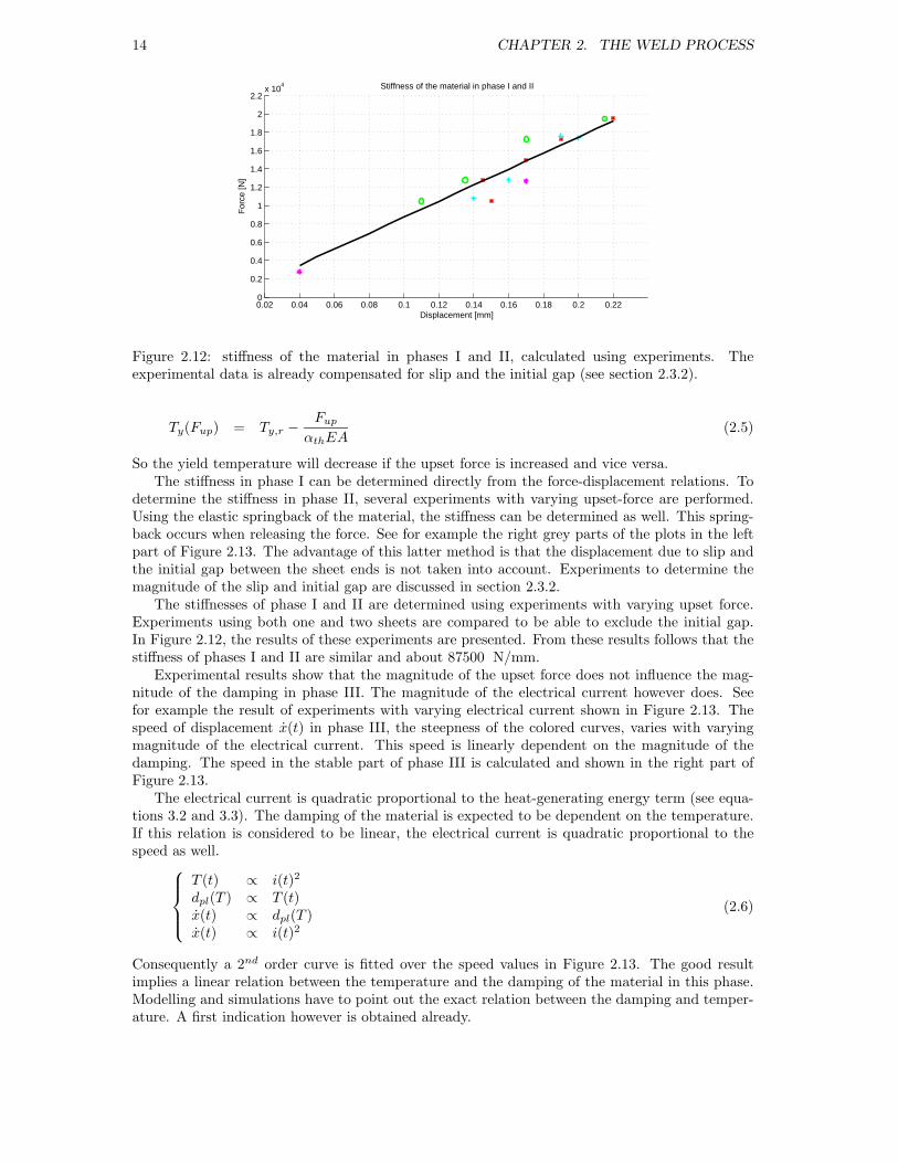
Figure 2.12: stiffness of the material in phases I and II, calculated using experiments. Theexperimental data is already compensated for slip and the initial gap (see section 2.3.2).
Ty(Fup) = Ty,r −Fup
αthEA(2.5)
So the yield temperature will decrease if the upset force is increased and vice versa.The stiffness in phase I can be determined directly from the force-displacement relations. To
determine the stiffness in phase II, several experiments with varying upset-force are performed.Using the elastic springback of the material, the stiffness can be determined as well. This spring-back occurs when releasing the force. See for example the right grey parts of the plots in the leftpart of Figure 2.13. The advantage of this latter method is that the displacement due to slip andthe initial gap between the sheet ends is not taken into account. Experiments to determine themagnitude of the slip and initial gap are discussed in section 2.3.2.
The stiffnesses of phase I and II are determined using experiments with varying upset force.Experiments using both one and two sheets are compared to be able to exclude the initial gap.In Figure 2.12, the results of these experiments are presented. From these results follows that thestiffness of phases I and II are similar and about 87500 N/mm.
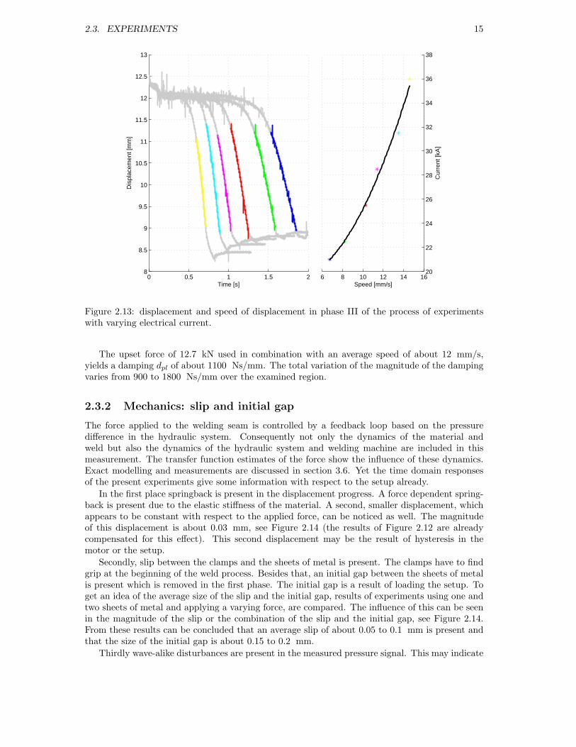
Experimental results show that the magnitude of the upset force does not influence the mag-nitude of the damping in phase III. The magnitude of the electrical current however does. Seefor example the result of experiments with varying electrical current shown in Figure 2.13. Thespeed of displacement x(t) in phase III, the steepness of the colored curves, varies with varyingmagnitude of the electrical current. This speed is linearly dependent on the magnitude of thedamping. The speed in the stable part of phase III is calculated and shown in the right part ofFigure 2.13.
The electrical current is quadratic proportional to the heat-generating energy term (see equa-tions 3.2 and 3.3). The damping of the material is expected to be dependent on the temperature.If this relation is considered to be linear, the electrical current is quadratic proportional to thespeed as well.
T (t) ∝ i(t)2
dpl(T ) ∝ T (t)x(t) ∝ dpl(T )x(t) ∝ i(t)2
(2.6)
Consequently a 2nd order curve is fitted over the speed values in Figure 2.13. The good resultimplies a linear relation between the temperature and the damping of the material in this phase.Modelling and simulations have to point out the exact relation between the damping and temper-ature. A first indication however is obtained already.
2.3. EXPERIMENTS 15
6 8 10 12 14 1620
22
24
26
28
30
32
34
36
38
Speed [mm/s]
Cur
rent
[kA
]
0 0.5 1 1.5 28
8.5
9
9.5
10
10.5
11
11.5
12
12.5
13
Dis
plac
emen
t [m
m]
Time [s]
Figure 2.13: displacement and speed of displacement in phase III of the process of experimentswith varying electrical current.
The upset force of 12.7 kN used in combination with an average speed of about 12 mm/s,yields a damping dpl of about 1100 Ns/mm. The total variation of the magnitude of the dampingvaries from 900 to 1800 Ns/mm over the examined region.
2.3.2 Mechanics: slip and initial gap
The force applied to the welding seam is controlled by a feedback loop based on the pressuredifference in the hydraulic system. Consequently not only the dynamics of the material andweld but also the dynamics of the hydraulic system and welding machine are included in thismeasurement. The transfer function estimates of the force show the influence of these dynamics.Exact modelling and measurements are discussed in section 3.6. Yet the time domain responsesof the present experiments give some information with respect to the setup already.
In the first place springback is present in the displacement progress. A force dependent spring-back is present due to the elastic stiffness of the material. A second, smaller displacement, whichappears to be constant with respect to the applied force, can be noticed as well. The magnitudeof this displacement is about 0.03 mm, see Figure 2.14 (the results of Figure 2.12 are alreadycompensated for this effect). This second displacement may be the result of hysteresis in themotor or the setup.
Secondly, slip between the clamps and the sheets of metal is present. The clamps have to findgrip at the beginning of the weld process. Besides that, an initial gap between the sheets of metalis present which is removed in the first phase. The initial gap is a result of loading the setup. Toget an idea of the average size of the slip and the initial gap, results of experiments using one andtwo sheets of metal and applying a varying force, are compared. The influence of this can be seenin the magnitude of the slip or the combination of the slip and the initial gap, see Figure 2.14.From these results can be concluded that an average slip of about 0.05 to 0.1 mm is present andthat the size of the initial gap is about 0.15 to 0.2 mm.
Thirdly wave-alike disturbances are present in the measured pressure signal. This may indicate
16 CHAPTER 2. THE WELD PROCESS
1 1.1 1.2 1.3 1.4 1.5 1.6 1.7 1.8 1.9 2
x 104
0
0.05
0.1
0.15
0.2
0.25
0.3
0.35Hysteresis, slip and inital gap in the weld process
Force [N]
Dis
plac
emen
t [m
m]
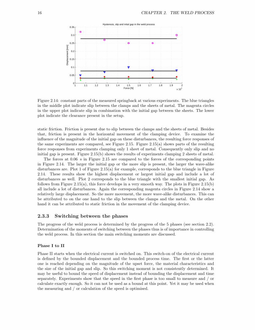
Figure 2.14: constant parts of the measured springback at various experiments. The blue trianglesin the middle plot indicate slip between the clamps and the sheets of metal. The magenta circlesin the upper plot indicate slip in combination with the initial gap between the sheets. The lowerplot indicate the clearance present in the setup.
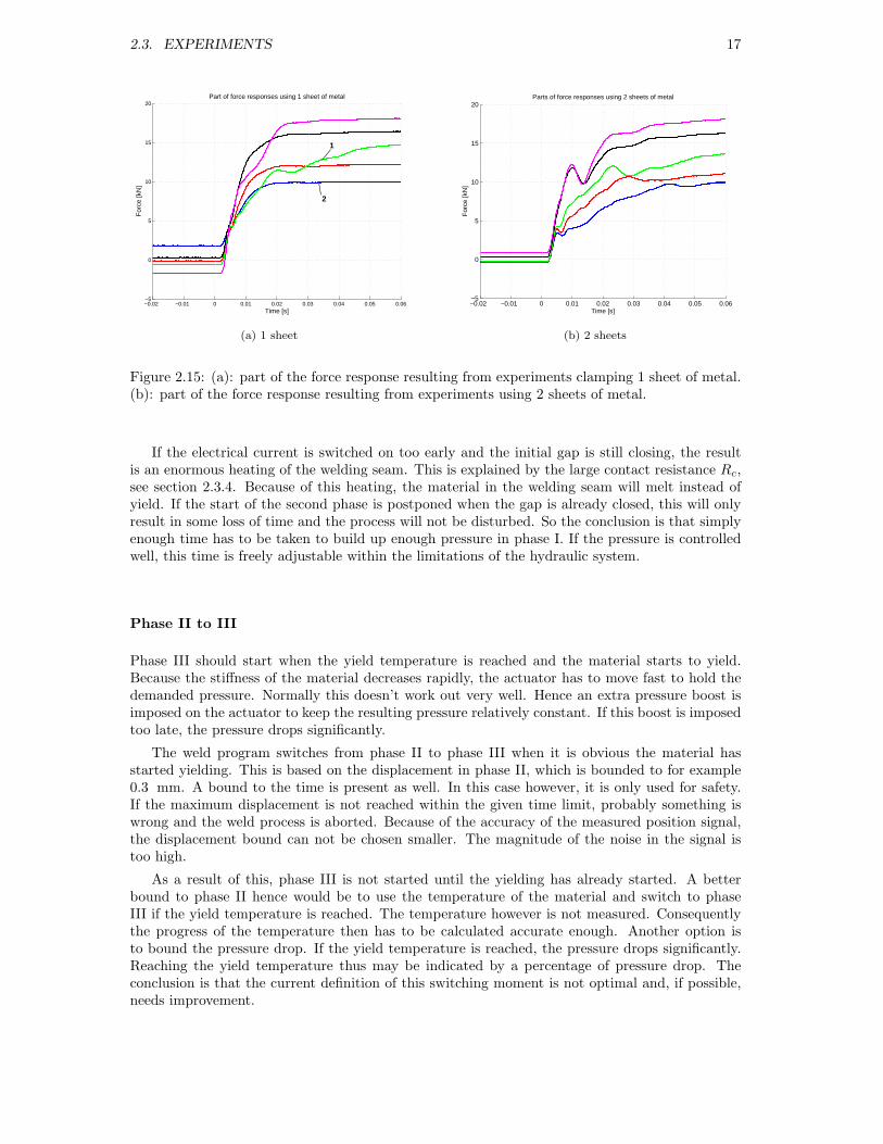
static friction. Friction is present due to slip between the clamps and the sheets of metal. Besidesthat, friction is present in the horizontal movement of the clamping device. To examine theinfluence of the magnitude of the initial gap on these disturbances, the resulting force responses ofthe same experiments are compared, see Figure 2.15. Figure 2.15(a) shows parts of the resultingforce responses from experiments clamping only 1 sheet of metal. Consequently only slip and noinitial gap is present. Figure 2.15(b) shows the results of experiments clamping 2 sheets of metal.
The forces at 0.06 s in Figure 2.15 are compared to the forces of the corresponding pointsin Figure 2.14. The larger the initial gap or the more slip is present, the larger the wave-alikedisturbances are. Plot 1 of Figure 2.15(a) for example, corresponds to the blue triangle in Figure2.14. These results show the highest displacement or largest initial gap and include a lot ofdisturbances as well. Plot 2 corresponds to the blue triangle with the smallest initial gap. Asfollows from Figure 2.15(a), this force develops in a very smooth way. The plots in Figure 2.15(b)all include a lot of disturbances. Again the corresponding magenta circles in Figure 2.14 show arelatively large displacement. So the more movement, the more wave-alike disturbances. This canbe attributed to on the one hand to the slip between the clamps and the metal. On the otherhand it can be attributed to static friction in the movement of the clamping device.
2.3.3 Switching between the phases
The progress of the weld process is determined by the progress of the 5 phases (see section 2.2).Determination of the moments of switching between the phases thus is of importance in controllingthe weld process. In this section the main switching moments are discussed.
Phase I to II
Phase II starts when the electrical current is switched on. This switch-on of the electrical currentis defined by the bounded displacement and the bounded process time. The first or the latterone is reached depending on the magnitude of the upset force, the material characteristics andthe size of the initial gap and slip. So this switching moment is not consistently determined. Itmay be useful to bound the speed of displacement instead of bounding the displacement and timeseparately. Experiments show that the speed in the first phase is too small to measure and / orcalculate exactly enough. So it can not be used as a bound at this point. Yet it may be used whenthe measuring and / or calculation of the speed is optimised.
2.3. EXPERIMENTS 17
−0.02 −0.01 0 0.01 0.02 0.03 0.04 0.05 0.06−5
0
5
10
15
20
Time [s]
For
ce [k
N]
Part of force responses using 1 sheet of metal
1
2
(a) 1 sheet
−0.02 −0.01 0 0.01 0.02 0.03 0.04 0.05 0.06−5
0
5
10
15
20
Time [s]
For
ce [k
N]
Parts of force responses using 2 sheets of metal
(b) 2 sheets
Figure 2.15: (a): part of the force response resulting from experiments clamping 1 sheet of metal.(b): part of the force response resulting from experiments using 2 sheets of metal.
If the electrical current is switched on too early and the initial gap is still closing, the resultis an enormous heating of the welding seam. This is explained by the large contact resistance Rc,see section 2.3.4. Because of this heating, the material in the welding seam will melt instead ofyield. If the start of the second phase is postponed when the gap is already closed, this will onlyresult in some loss of time and the process will not be disturbed. So the conclusion is that simplyenough time has to be taken to build up enough pressure in phase I. If the pressure is controlledwell, this time is freely adjustable within the limitations of the hydraulic system.
Phase II to III
Phase III should start when the yield temperature is reached and the material starts to yield.Because the stiffness of the material decreases rapidly, the actuator has to move fast to hold thedemanded pressure. Normally this doesn’t work out very well. Hence an extra pressure boost isimposed on the actuator to keep the resulting pressure relatively constant. If this boost is imposedtoo late, the pressure drops significantly.
The weld program switches from phase II to phase III when it is obvious the material hasstarted yielding. This is based on the displacement in phase II, which is bounded to for example0.3 mm. A bound to the time is present as well. In this case however, it is only used for safety.If the maximum displacement is not reached within the given time limit, probably something iswrong and the weld process is aborted. Because of the accuracy of the measured position signal,the displacement bound can not be chosen smaller. The magnitude of the noise in the signal istoo high.
As a result of this, phase III is not started until the yielding has already started. A betterbound to phase II hence would be to use the temperature of the material and switch to phaseIII if the yield temperature is reached. The temperature however is not measured. Consequentlythe progress of the temperature then has to be calculated accurate enough. Another option isto bound the pressure drop. If the yield temperature is reached, the pressure drops significantly.Reaching the yield temperature thus may be indicated by a percentage of pressure drop. Theconclusion is that the current definition of this switching moment is not optimal and, if possible,needs improvement.
18 CHAPTER 2. THE WELD PROCESS
Phase III to IV
The switching moment between phase III to IV is defined by the demanded amount of upset. Ifthe displacement bound is reached, the electrical current is switched off and the upset force isdiminished to stop the yielding of the material. The duration of phase III can be influenced byvarying the magnitude of the electrical current i(t) and of the force F (t) (see section 2.3.5). Thedisadvantage is that the process is not forced to stop yielding. The material has to cool down first.So a fluctuation in the final displacement may occur and most times overshoot in the displacementis present.
2.3.4 Contact and bulk resistance
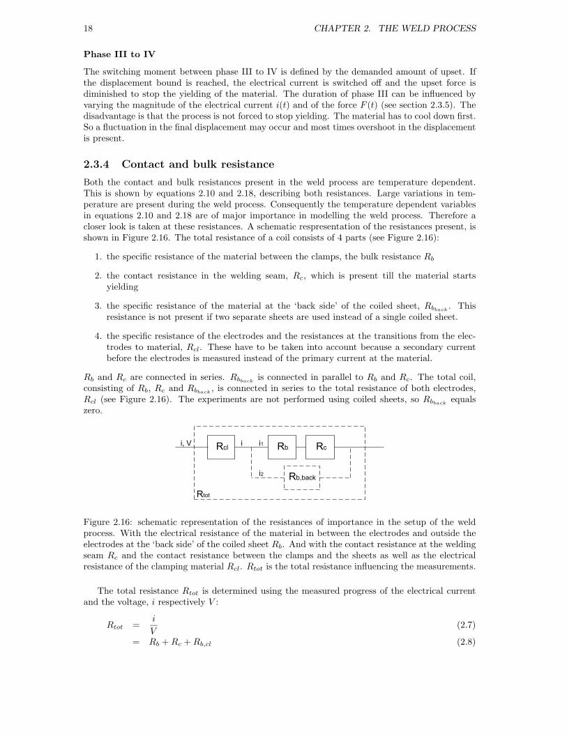
Both the contact and bulk resistances present in the weld process are temperature dependent.This is shown by equations 2.10 and 2.18, describing both resistances. Large variations in tem-perature are present during the weld process. Consequently the temperature dependent variablesin equations 2.10 and 2.18 are of major importance in modelling the weld process. Therefore acloser look is taken at these resistances. A schematic respresentation of the resistances present, isshown in Figure 2.16. The total resistance of a coil consists of 4 parts (see Figure 2.16):
1. the specific resistance of the material between the clamps, the bulk resistance Rb
2. the contact resistance in the welding seam, Rc, which is present till the material startsyielding
3. the specific resistance of the material at the ‘back side’ of the coiled sheet, Rbback. This
resistance is not present if two separate sheets are used instead of a single coiled sheet.
4. the specific resistance of the electrodes and the resistances at the transitions from the elec-trodes to material, Rcl. These have to be taken into account because a secondary currentbefore the electrodes is measured instead of the primary current at the material.
Rb and Rc are connected in series. Rbbackis connected in parallel to Rb and Rc. The total coil,
consisting of Rb, Rc and Rbback, is connected in series to the total resistance of both electrodes,
Rcl (see Figure 2.16). The experiments are not performed using coiled sheets, so Rbbackequals
zero.
Rcl Rb Rc
Rtot
Rb,back
i, V
i2
i . i1
Figure 2.16: schematic representation of the resistances of importance in the setup of the weldprocess. With the electrical resistance of the material in between the electrodes and outside theelectrodes at the ‘back side’ of the coiled sheet Rb. And with the contact resistance at the weldingseam Rc and the contact resistance between the clamps and the sheets as well as the electricalresistance of the clamping material Rcl. Rtot is the total resistance influencing the measurements.
The total resistance Rtot is determined using the measured progress of the electrical currentand the voltage, i respectively V :
Rtot =i
V(2.7)
= Rb + Rc + Rb,cl (2.8)
2.3. EXPERIMENTS 19
Using one sheet of metal instead of two, the contact resistance Rc in equation 2.8 is eliminated.Rsub is defined as the resistance of the sheets and the clamps together. Making use of the samerelation as in equation 2.7 the magnitude of this resistance is determined
Rsub = Rb + Rcl (2.9)
Rcl is constant, while Rb is dependent on the distance L between the clamps. By varying thisdistance between the clamps and applying a constant force and electrical current, Rb and Rcl aredetermined separately [Bejan, 1993], [Wolfram, (web)]
Rb = ρe(T )L
dydz(2.10)
with ρe(T ) the temperature dependent electrical resistivity of the material in Ωm [Bejan,1993],[Wolfram, (web)]
ρe = ρe,r(1 + αρ(T − Tr)) (2.11)
= ρe,r
T
Tr
for αρ = 3.35 · 10−3
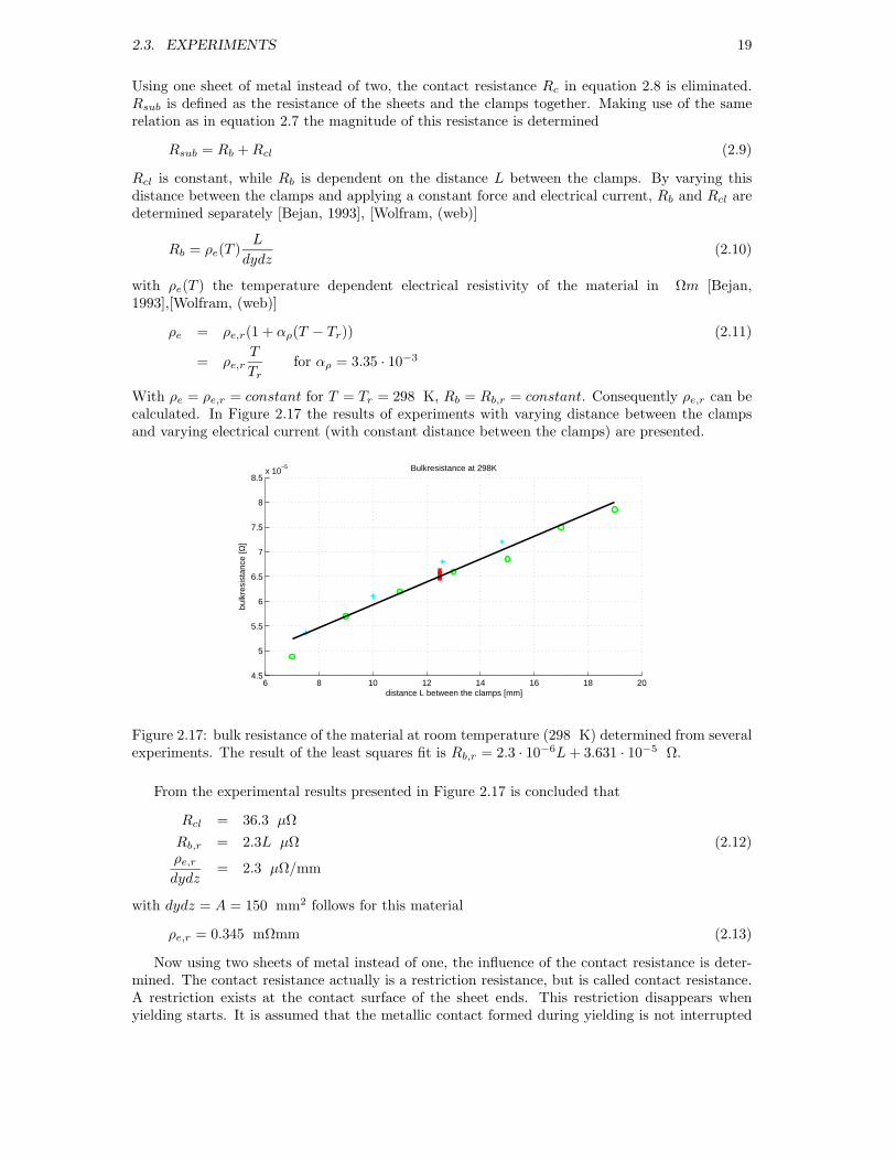
With ρe = ρe,r = constant for T = Tr = 298 K, Rb = Rb,r = constant. Consequently ρe,r can becalculated. In Figure 2.17 the results of experiments with varying distance between the clampsand varying electrical current (with constant distance between the clamps) are presented.
6 8 10 12 14 16 18 204.5
5
5.5
6
6.5
7
7.5
8
8.5x 10
−5 Bulkresistance at 298K
distance L between the clamps [mm]
bulk
resi
stan
ce [Ω
]
Figure 2.17: bulk resistance of the material at room temperature (298 K) determined from severalexperiments. The result of the least squares fit is Rb,r = 2.3 · 10−6L + 3.631 · 10−5 Ω.
From the experimental results presented in Figure 2.17 is concluded that
Rcl = 36.3 µΩ
Rb,r = 2.3L µΩ (2.12)ρe,r
dydz= 2.3 µΩ/mm
with dydz = A = 150 mm2 follows for this material
ρe,r = 0.345 mΩmm (2.13)
Now using two sheets of metal instead of one, the influence of the contact resistance is deter-mined. The contact resistance actually is a restriction resistance, but is called contact resistance.A restriction exists at the contact surface of the sheet ends. This restriction disappears whenyielding starts. It is assumed that the metallic contact formed during yielding is not interrupted

20 CHAPTER 2. THE WELD PROCESS
anymore. So once the contact resistance is gone, it does not come back anymore (see also section3.3.2). Zwolsman [1987] modelled the contact resistance using
Rc =ρe
2ao
(2.14)
with ao the radius of an imaginary circle describing the metallic contact area in between the twosheet ends. The electrical current and heat flows are assumed to follow the same paths. Nextthe surface pressure is assumed to be equal to the Brinell Hardness. However this is only trueat the breaking stress of the material. Consequently Zwolsman introduces a compensation factorξZm = 3
σsurf =F
πa2o
(2.15)
=1
ξZm
HB (2.16)
Taking into account the temperature dependency of HB and ρe (eq. 2.11), a theoretical modelfor the contact resistance results:
HB(t) = HBr
Ty − T (t)
Ty − Tr
(2.17)
Rc(t) =ρe,r
2
√
π
ξZm
HBr
F (t)
Ty − T (t)
Ty − Tr
T (t)
Tr
(2.18)
∝ F (t)−0.5 (2.19)
The total resistance is calculated using the measured voltage and electrical current at theswitch-on of the electrical current. In this way the temperature will still be about room tempera-ture and the previous calculated Rb,r and Rcl can be used to determine Rc,r. In Figure 2.18 thecontact resistance resulting from the theory using equation 2.18 as well as the contact resistanceresulting from corresponding experiments are shown (see also section 3.3.2).
0.9 1 1.1 1.2 1.3 1.4 1.5 1.6 1.7 1.8 1.9
x 104
2
3
4
5
6
7
8x 10
−5 Contact resistance at 298K
Force [N]
Res
ista
nce
[Ω]
Figure 2.18: contact resistance of the welding seam. The green circles indicate the measurementsresults, while the red blocks indicate the theoretical values. The result of the least squares fit overthe measurements is Rc = 0.022F−0.68 Ω
From the theory it follows that Rc ∝ F−0.5 (equation 2.19), while the experimentally deter-mined Rc is proportional to F−0.68. This is a relatively good comparable result (see Figure 2.18).However the absolute value of the theoretical Rc is about twice as high as the experimental values.
2.3. EXPERIMENTS 21
Zwolsman compensates in the derivation of equation 2.18 for some discrepancy between his the-ory and experimental results using factors based on experiments and making some assumptions.Furthermore the theory is tested with wires of Cu, MnNi and Mo while in this case sheets of steelare used. Hence his compensation factor ξZm, used in equation 2.18, is adjusted for this particularprocess:
ξURW = 22ξZm (2.20)
= 12
When rims or coils are welded instead of small sheets of metal, Rbbackwill also be present. To
examine the influence of this extra resistance on the process, an indication for the magnitude ofRbback
is calculated. The magnitude of Rbbackdepends on the diameter of the rim and the size of
the cross section of the metal used. The larger the diameter or the smaller the cross section, thelarger Rbback
will be and vice versa. Normally, the width of a rim varies from about 200 to 500 mm.The thickness of the material may vary from 2 to 8 mm. And the size of the circumference variesfrom about 1000 to 1800 mm. The thinnest material off course won’t be used for the larger rimsand the thickest material not for the smaller rims, so an average of each variable is used. Thisresults in a cross section of 1750 mm2 and a circumference of 1400 mm. Using equations 2.10and 2.13 this results in a resistance at room temperature of 0.28 mΩ if the same material as inthese experiments is used. The maximum magnitude of the bulk resistance of the weld region atroom temperature is assumed to be about 5 µΩ (for this cross section). The maximum magnitudeof the contact resistance in the welding seam at room temperature is assumed to be about and50 µΩ. The contact resistance is independent on the cross section, because of the dependence onthe force instead of the pressure. The total resistance of the weld region at room temperature,Rb,r + Rc, will be about 55 µΩ. Using the following equations which result from Figure 2.16
V = i1(Rb,r + Rc) = i2Rbback,r (2.21)
i1i2
=Rbback,r
Rb,r + Rc
(2.22)
it follows that under these conditions i1 will be about 5 times as high as i2. When temperatureincreases, the resistances increase as well. The weld temperature of the welding seam will becomeabout 1500 K while the temperature of the back side of the coil will only be slightly above roomtemperature. Combining equations 2.10, 2.13 and 2.22 it follows that i1 will be about 70 timesas high as i2 under these conditions. So the loss of electrical current through the back side ofthe coil will be relatively high in the beginning of the weld process. In a later stage of the weldprocess, when only bulk resistance is present in between the clamps, the loss of electrical currentwill be small. The result is a minimal increase in temperature of the back side of the coil, whichis neglegible.
2.3.5 Time of the weld process
The time the total weld process takes is mainly determined by the duration of the heating andyielding phases. The first one is bounded by reaching the yield temperature of the material. Thelatter one is bounded by the demanded amount of upset. The height of the yield temperatureis influenced by the applied upset force. The smaller the magnitude of this force, the higher theyield temperature (see Figure 2.11). However if too less force is used, the contact resistance will behigher and heat is generated more quickly. The speed of heating of the material is also dependenton the amount of heat generation. This amount is influenced by the magnitude of the appliedelectrical current. So the duration of phase II depends both on the magnitude of the force andthe magnitude of the electrical current.
22 CHAPTER 2. THE WELD PROCESS
1 1.1 1.2 1.3 1.4 1.5 1.6 1.7 1.8 1.9 2
x 104
0.2
0.3
0.4
0.5
0.6
0.7
0.8
0.9
1
1.1
1.2
Force(set) [N]
Tim
e pe
r ph
ase
[s]
Influence of the force on the time per phase
Phase II + III
Phase II
Phase III
(a) force vs time
1.8 2 2.2 2.4 2.6 2.8 3
x 104
0.2
0.4
0.6
0.8
1
1.2
1.4
1.6
1.8Influence of the current on the time per phase
Current (mean of phase II and II) [A]
Tim
e pe
r ph
ase
[s]
Phase III
Phase II
Phase II + III
(b) electrical current vs time
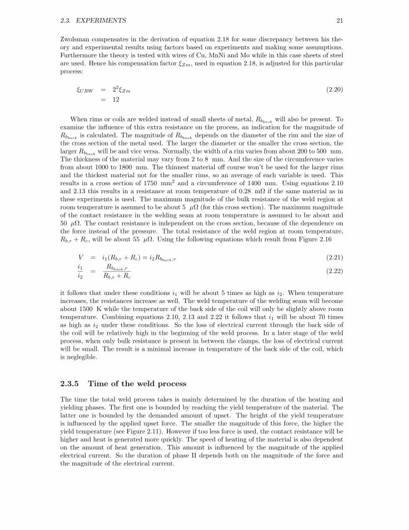
Figure 2.19: (a): Influence of the upset force on the duration of the various phases of the weldprocess. (b): Influence of the magnitude of the electrical current on the duration of the variousphases of the weld process.
The relation between the duration of phase II and the magnitude of the force and the electricalcurrent is examined. Thus experiments with varying force and electrical current are performed.The influence of the upset force on the duration of this phase is depicted in Figure 2.19(a). Themiddle (green) plot shows the duration of the heating phase for varying magnitudes of the upset-force. As expected, it is nonlinear because of the influence of the upset-force on the contactresistance as well as on the magnitude of the yield temperature. The duration of phase III (thelower (red) plot) on the other hand, is decreased because of the relatively low force. If the forceis increased, the yield temperature will decrease. This results in a relatively short heating period,but also in a relatively low temperature during yielding. So the duration of phase II decreases,while the duration of phase III increases. As a result of this, the duration of phase III with respectto the duration of phase II can be manipulated.
Figure 2.19(a) shows that phase II has maximum duration if an upset force of about 15 kNis used. At the same point phase III has minimum duration. If the the magnitude of the upsetforce is increased, the total weld time decreases (the upper (blue) plot in Figure 2.19(a)). Theconclusing is that the influence of the decreased yield temperature is more significant than theinfluence of the increased contact surface.
The influence of the magnitude of the electrical current on the process time is depicted inFigure 2.19(b). As expected, the larger the magnitude of the electrical current, the shorter theduration of the process. The larger the magnitude of the electrical current, the higher the energygeneration and heating of the material. Consequently the yield temperature will be reached soonerand the duration of phase II decreases. Moreover the material can be heated more rapidly to theyield temperature during yielding and the duration of phase III decreases as well.
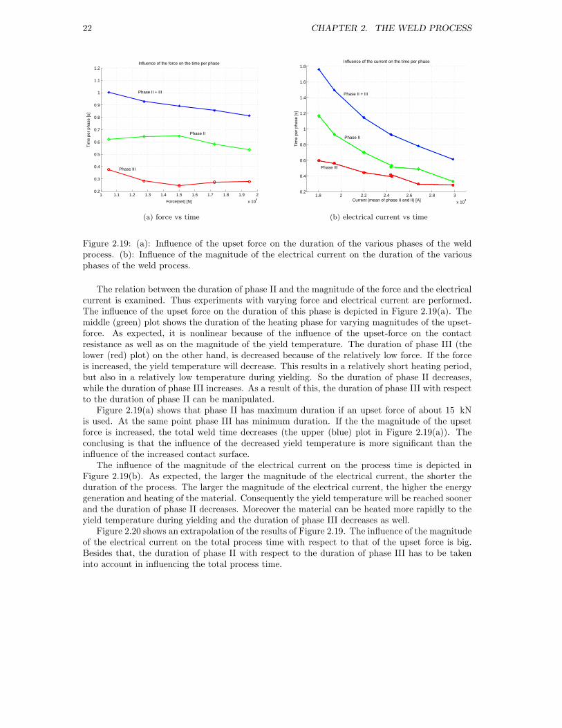
Figure 2.20 shows an extrapolation of the results of Figure 2.19. The influence of the magnitudeof the electrical current on the total process time with respect to that of the upset force is big.Besides that, the duration of phase II with respect to the duration of phase III has to be takeninto account in influencing the total process time.
2.3. EXPERIMENTS 23
1
2
3x 10
4
11.5
2
x 104
0.4
0.6
0.8
1
Force [N]
Phase II (heating)
Current [A]
Tim
e [s
]
1
2
3x 10
4
11.5
2
x 104
0.2
0.3
0.4
0.5
Force [N]
Phase III (yielding)
Current [A]
Tim
e [s
]
1
2
3x 10
4
11.5
2
x 104
0.5
1
1.5
Force [N]
Phase II & III
Current [A]
Tim
e [s
]
1
2
3x 10
4
11.5
2
x 104
1
1.5
2
Force [N]
Total process
Current [A]
Tim
e [s
]
1.1
1.2
1.3
1.4
1.5
0.3
0.35
0.4
0.45
Figure 2.20: influence of the magnitude of the electrical current and the upset force on the durationof the various phases in the process and on the total process time.

24 CHAPTER 2. THE WELD PROCESS
Chapter 3
Modelling
3.1 Introduction
The theory of the weld process is validated partly by the experiments as described in section2.3. To complete the theory, a model of the process is derived. First an inventory of previouslyperformed modelling and the goals in modelling the weld process are discussed. Next the processis divided into several parts. An overview of the modelling per part is given after which theyare combined to a single model. In Appendix B a description of the resulting simulation model,which can be used for off-line simulation of the weld process, is included. Finally the derivedmodel is validated by experimental results. Furthermore, the modelling of the hydraulic system ispresented in Appendix C. The results are presented in section 3.6.
3.1.1 Previous modelling
A number of studies trying to model the weld process have been performed already. Meulenberg[2002] and Put [1999] both modelled the thermodynamical part of the process for example. Meu-lenberg [2002] focussed on the heating of the material and Put [1999] paid special attention tothe cooling down of the material. Both divided the working area into several distinctive sections.Next they derived a discretisised model of the working area, coupling the sections by the use ofthe corresponding balance of energy per section. A clear overview of the systems and equilibriapresent in the weld process as well as the assumptions done in modelling the process, are missing.Consequently parts are missing in their modelling as well. The resulting models do not give asatisfactory representation of (parts of) the weld process. Hence in this study, this is discussedextensively (see section 2.2). Besides that, at Put’s work it is very indistinct what his final modellooks like due to a lack of structure and overview. Other studies on modelling of the DC upsetresistance weld process as performed on the FRW-series are Elassal [1996] and Legemaate [1998].Studies on resistance spot welding like Feng [1998] are considered also. However these studiescontribute more to the insight in the process, than really being a guide for modelling the weldprocess discussed in this study.
The weld process consists of a thermodynamical and a mechanical part. The thermodynamicalbehaviour and the mechanical behaviour of the process are coupled and thus influence each other.Consequently both parts have to be considered to gain good insight in the process. Until nowmost of the performed research was only focussed on the thermodynamical part of the process.Only Elassal [1996] focussed on the mechanics of the welding machine. However he paid littleattention to thermodynamical part of the process. Meulenberg [2002] was the first one to startthinking of a mass-spring-damper system describing the mechanics of the weld process. Howeverhe didn’t succeed in modelling it adequately.
So most of the existing modelling only involves parts of the complete weld process. Besidesthat, the modelled parts present in previous studies are incomplete due to a lack of insight inthe process. Energy loss through yielding for example, has not been used in previous modelling.
25
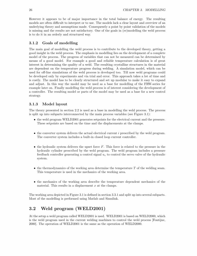
26 CHAPTER 3. MODELLING
However it appears to be of major importance in the total balance of energy. The resultingmodels are often difficult to interpret or to use. The models lack a clear layout and overview of anunderlying theory and assumptions made. Consequently a point by point validation of the modelsis missing and the results are not satisfactory. One of the goals in (re)modelling the weld processis to do it in an orderly and structured way.
3.1.2 Goals of modelling
The main goal of modelling the weld process is to contribute to the developed theory, getting agood insight in the weld process. The emphasis in modelling lies on the development of a completemodel of the process. The progress of variables that can not be measured can be determined bymeans of a good model. For example a good and reliable temperature calculation is of greatinterest in determining the quality of a weld. The resulting crystalline structures in the materialare dependent on the temperature progress during welding. A simulation model, which can beused for off-line simulations of the weld process is developed too. Till now weld programs couldbe developed only by experiments and via trial and error. This approach takes a lot of time andis costly. The model has to be clearly structured and set up modular to make it easy to expandand adjust. In this way the model may be used as a base for modelling of the FRW-series forexample later on. Finally modelling the weld process is of interest considering the development ofa controller. The resulting model or parts of the model may be used as a base for a new controlstrategy.
3.1.3 Model layout
The theory presented in section 2.2 is used as a base in modelling the weld process. The processis split up into subparts interconnected by the main process variables (see Figure 3.1):
• the weld program WELD2001 generates setpoints for the electrical current and the pressure.These setpoints are based on the time and the displacements at the clamps.
• the converter system delivers the actual electrical current i prescribed by the weld program.The converter system includes a built-in closed loop current controller.
• the hydraulic system delivers the upset force F . This force is related to the pressure in thehydraulic cylinder prescribed by the weld program. The weld program includes a pressurefeedback controller generating a control signal uv to control the servo valve of the hydraulicsystem.
• the thermodynamics of the working area determine the temperature T of the welding seam.This temperature is used in the mechanics of the working area.
• the mechanics of the working area describe the temperature dependent mechanics of thematerial. This results in a displacement x at the clamps.
The working area depicted in Figure 3.1 is defined in section 3.3.1 and split up into several subparts.Most of the modelling is performed using Matlab and Simulink.
3.2 Weld program (WELD2001)
At the setup a weld program called WELD2001 is used. WELD2001 is based on WELD2000, whichis the weld program used in the current welding machines to control the weld process [Fontijne,2000]. The operation of WELD2001 is the same as the operation of WELD2000.
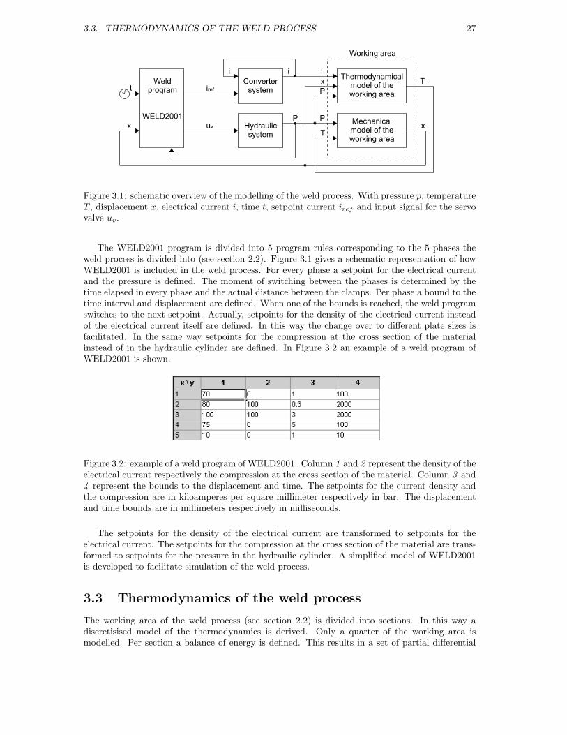
3.3. THERMODYNAMICS OF THE WELD PROCESS 27
Thermodynamicalmodel of theworking area
Convertersystem
Mechanicalmodel of theworking area
Hydraulicsystem
iref
uv
Weldprogram
WELD2001
xP
Tt
i i
Tx
P
P
x
i
Working area
Figure 3.1: schematic overview of the modelling of the weld process. With pressure p, temperatureT , displacement x, electrical current i, time t, setpoint current iref and input signal for the servovalve uv.
The WELD2001 program is divided into 5 program rules corresponding to the 5 phases theweld process is divided into (see section 2.2). Figure 3.1 gives a schematic representation of howWELD2001 is included in the weld process. For every phase a setpoint for the electrical currentand the pressure is defined. The moment of switching between the phases is determined by thetime elapsed in every phase and the actual distance between the clamps. Per phase a bound to thetime interval and displacement are defined. When one of the bounds is reached, the weld programswitches to the next setpoint. Actually, setpoints for the density of the electrical current insteadof the electrical current itself are defined. In this way the change over to different plate sizes isfacilitated. In the same way setpoints for the compression at the cross section of the materialinstead of in the hydraulic cylinder are defined. In Figure 3.2 an example of a weld program ofWELD2001 is shown.
Figure 3.2: example of a weld program of WELD2001. Column 1 and 2 represent the density of theelectrical current respectively the compression at the cross section of the material. Column 3 and4 represent the bounds to the displacement and time. The setpoints for the current density andthe compression are in kiloamperes per square millimeter respectively in bar. The displacementand time bounds are in millimeters respectively in milliseconds.
The setpoints for the density of the electrical current are transformed to setpoints for theelectrical current. The setpoints for the compression at the cross section of the material are trans-formed to setpoints for the pressure in the hydraulic cylinder. A simplified model of WELD2001is developed to facilitate simulation of the weld process.
3.3 Thermodynamics of the weld process
The working area of the weld process (see section 2.2) is divided into sections. In this way adiscretisised model of the thermodynamics is derived. Only a quarter of the working area ismodelled. Per section a balance of energy is defined. This results in a set of partial differential
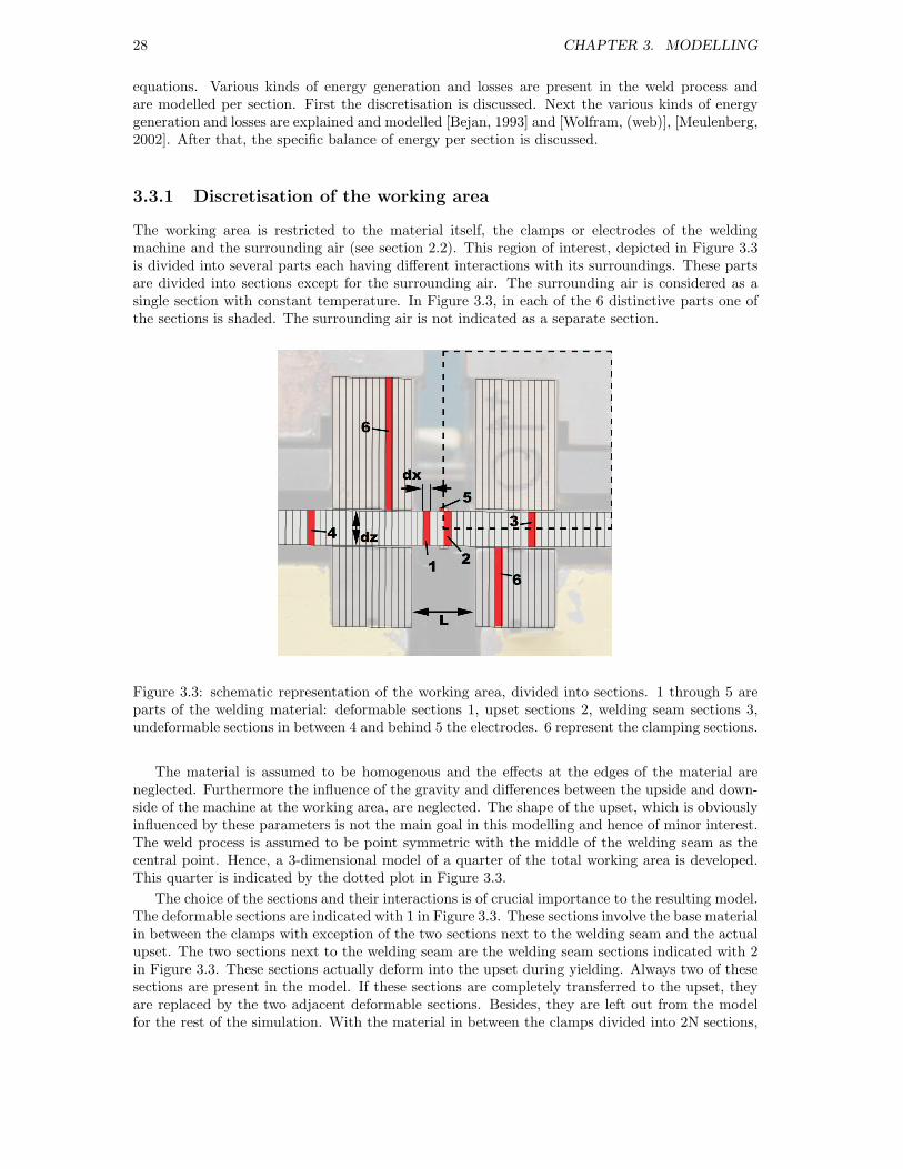
28 CHAPTER 3. MODELLING
equations. Various kinds of energy generation and losses are present in the weld process andare modelled per section. First the discretisation is discussed. Next the various kinds of energygeneration and losses are explained and modelled [Bejan, 1993] and [Wolfram, (web)], [Meulenberg,2002]. After that, the specific balance of energy per section is discussed.
3.3.1 Discretisation of the working area
The working area is restricted to the material itself, the clamps or electrodes of the weldingmachine and the surrounding air (see section 2.2). This region of interest, depicted in Figure 3.3is divided into several parts each having different interactions with its surroundings. These partsare divided into sections except for the surrounding air. The surrounding air is considered as asingle section with constant temperature. In Figure 3.3, in each of the 6 distinctive parts one ofthe sections is shaded. The surrounding air is not indicated as a separate section.
Figure 3.3: schematic representation of the working area, divided into sections. 1 through 5 areparts of the welding material: deformable sections 1, upset sections 2, welding seam sections 3,undeformable sections in between 4 and behind 5 the electrodes. 6 represent the clamping sections.
The material is assumed to be homogenous and the effects at the edges of the material areneglected. Furthermore the influence of the gravity and differences between the upside and down-side of the machine at the working area, are neglected. The shape of the upset, which is obviouslyinfluenced by these parameters is not the main goal in this modelling and hence of minor interest.The weld process is assumed to be point symmetric with the middle of the welding seam as thecentral point. Hence, a 3-dimensional model of a quarter of the total working area is developed.This quarter is indicated by the dotted plot in Figure 3.3.
The choice of the sections and their interactions is of crucial importance to the resulting model.The deformable sections are indicated with 1 in Figure 3.3. These sections involve the base materialin between the clamps with exception of the two sections next to the welding seam and the actualupset. The two sections next to the welding seam are the welding seam sections indicated with 2in Figure 3.3. These sections actually deform into the upset during yielding. Always two of thesesections are present in the model. If these sections are completely transferred to the upset, theyare replaced by the two adjacent deformable sections. Besides, they are left out from the modelfor the rest of the simulation. With the material in between the clamps divided into 2N sections,
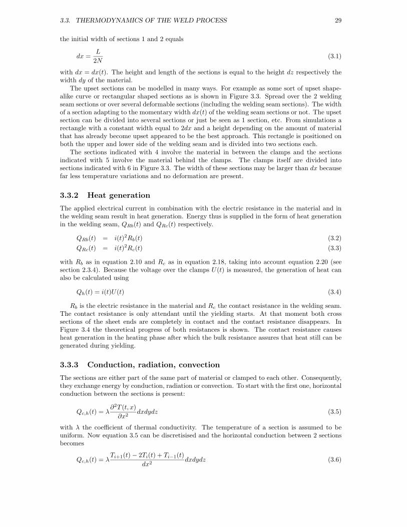
3.3. THERMODYNAMICS OF THE WELD PROCESS 29
the initial width of sections 1 and 2 equals
dx =L
2N(3.1)
with dx = dx(t). The height and length of the sections is equal to the height dz respectively thewidth dy of the material.
The upset sections can be modelled in many ways. For example as some sort of upset shape-alike curve or rectangular shaped sections as is shown in Figure 3.3. Spread over the 2 weldingseam sections or over several deformable sections (including the welding seam sections). The widthof a section adapting to the momentary width dx(t) of the welding seam sections or not. The upsetsection can be divided into several sections or just be seen as 1 section, etc. From simulations arectangle with a constant width equal to 2dx and a height depending on the amount of materialthat has already become upset appeared to be the best approach. This rectangle is positioned onboth the upper and lower side of the welding seam and is divided into two sections each.
The sections indicated with 4 involve the material in between the clamps and the sectionsindicated with 5 involve the material behind the clamps. The clamps itself are divided intosections indicated with 6 in Figure 3.3. The width of these sections may be larger than dx becausefar less temperature variations and no deformation are present.
3.3.2 Heat generation
The applied electrical current in combination with the electric resistance in the material and inthe welding seam result in heat generation. Energy thus is supplied in the form of heat generationin the welding seam, QRb(t) and QRc(t) respectively.
QRb(t) = i(t)2Rb(t) (3.2)
QRc(t) = i(t)2Rc(t) (3.3)
with Rb as in equation 2.10 and Rc as in equation 2.18, taking into account equation 2.20 (seesection 2.3.4). Because the voltage over the clamps U(t) is measured, the generation of heat canalso be calculated using
Qh(t) = i(t)U(t) (3.4)
Rb is the electric resistance in the material and Rc the contact resistance in the welding seam.The contact resistance is only attendant until the yielding starts. At that moment both crosssections of the sheet ends are completely in contact and the contact resistance disappears. InFigure 3.4 the theoretical progress of both resistances is shown. The contact resistance causesheat generation in the heating phase after which the bulk resistance assures that heat still can begenerated during yielding.
3.3.3 Conduction, radiation, convection
The sections are either part of the same part of material or clamped to each other. Consequently,they exchange energy by conduction, radiation or convection. To start with the first one, horizontalconduction between the sections is present:
Qc,h(t) = λ∂2T (t, x)
∂x2dxdydz (3.5)
with λ the coefficient of thermal conductivity. The temperature of a section is assumed to beuniform. Now equation 3.5 can be discretisised and the horizontal conduction between 2 sectionsbecomes
Qc,h(t) = λTi+1(t) − 2Ti(t) + Ti−1(t)
dx2dxdydz (3.6)
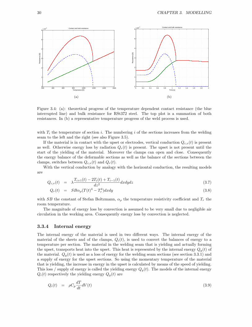
30 CHAPTER 3. MODELLING
200 400 600 800 1000 1200 1400 16000
1
2
3
4
5
6x 10
−5 Contact and bulk resistance
Temperature [K]
Res
ista
nce
[Ω]
(a)
0 0.2 0.4 0.6 0.8 1 1.2 1.4 1.6 1.8 20
1
2
3
4
5
6x 10
−5 Contact and bulk resistance
Time [s]
Res
ista
nce
[Ω]
(b)
Figure 3.4: (a): theoretical progress of the temperature dependent contact resistance (the blueinterrupted line) and bulk resistance for RSt372 steel. The top plot is a summation of bothresistances. In (b) a representative temperature progress of the weld process is used.
with Ti the temperature of section i. The numbering i of the sections increases from the weldingseam to the left and the right (see also Figure 3.5).
If the material is in contact with the upset or electrodes, vertical conduction Qc,v(t) is presentas well. Otherwise energy loss by radiation Qr(t) is present. The upset is not present until thestart of the yielding of the material. Moreover the clamps can open and close. Consequentlythe energy balance of the deformable sections as well as the balance of the sections between theclamps, switches between Qc,v(t) and Qr(t).
With the vertical conduction by analogy with the horizontal conduction, the resulting modelsare
Qc,v(t) = λTi+1(t) − 2Ti(t) + Ti−1(t)
dz2dxdydz (3.7)
Qr(t) = SBαρ(T (t)4 − T 4r )dxdy (3.8)
with SB the constant of Stefan Boltzmann, αρ the temperature resistivity coefficient and Tr theroom temperature.
The magnitude of energy loss by convection is assumed to be very small due to negligible aircirculation in the working area. Consequently energy loss by convection is neglected.
3.3.4 Internal energy
The internal energy of the material is used in two different ways. The internal energy of thematerial of the sheets and of the clamps, Qi(t), is used to convert the balances of energy to atemperature per section. The material in the welding seam that is yielding and actually formingthe upset, transports heat into the upset. This heat is represented by the internal energy Qy(t) ofthe material. Qy(t) is used as a loss of energy for the welding seam sections (see section 3.3.1) anda supply of energy for the upset sections. So using the momentary temperature of the materialthat is yielding, the increase in energy in the upset is calculated by means of the speed of yielding.This loss / supply of energy is called the yielding energy Qy(t). The models of the internal energyQi(t) respectively the yielding energy Qy(t) are
Qi(t) = ρCp
dT
dtdV (t) (3.9)

3.3. THERMODYNAMICS OF THE WELD PROCESS 31
Qy(t) = ρCpT (t)dV (t)
dt(3.10)
= ρCpT (t)dx(t)dydz
with ρ the specific mass, Cp the specific heat of the material and dx(t) = dx(t)dt
the speed ofdeformation. The specific heat is a temperature dependent parameter. For steel 1010, which is arepresentative material, holds
Cp = 420 + 0, 47(T (t) − 273, 15) (3.11)
3.3.5 Balances of energy
Six distinctive sections are present in the schematic representation of Figure 3.3. This divisionis among other things, based on the specific supply of energy Qs(t) and loss of energy Ql(t) persection. These supply and loss of energy are used in the specific balance of energy per section. InFigure 3.5 an example of a welding seam section is shown.
Figure 3.5: schematic representation of a welding seam section.
Analogous to the numbering in Figure 3.3 follows:
section 1 the deformable sections with Qi(t), QRb(t), Qc,h(t) and Qr(t). If these sections becomewelding seam sections and start to yield (see section 3.3.1), Qr(t) changes into Qc,v(t) andQy(t).
section 2 the welding seam sections have got the same energy terms as the deformable sections.However, the radiation term Qr(t) changes to Qc,v(t) and Qy(t) if yielding starts. Besides,till yielding starts, extra heat generation QRc(t) is present (see section 3.3.2).
section 3 the non-deformable sections between the clamps with Qi(t), Qc,h(t) and till the weldprogram is ended, Qc,v(t). If the program is ended and the clamps are opened, this latterterm becomes Qr(t).
section 4 the non-deformable sections behind the clamps with Qi(t), Qc,h(t) and Qr(t).
section 5 the upset sections include Qi(t), Qc,v(t), Qr(t) and Qy(t). Is is assumed no energygeneration QRb(t) takes place in the upset.
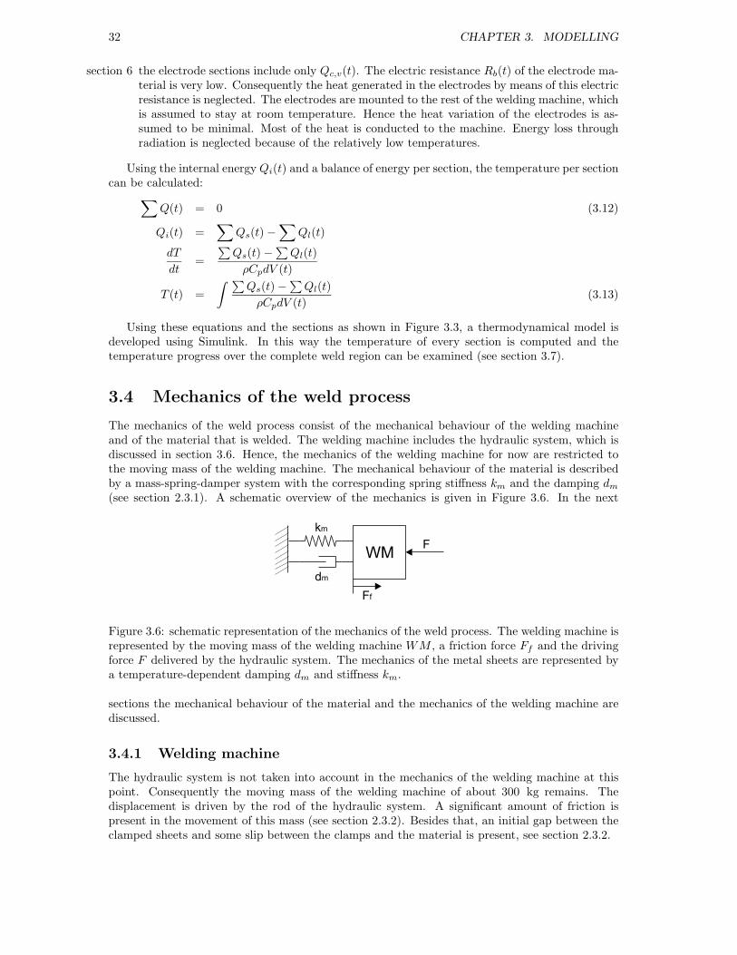
32 CHAPTER 3. MODELLING
section 6 the electrode sections include only Qc,v(t). The electric resistance Rb(t) of the electrode ma-terial is very low. Consequently the heat generated in the electrodes by means of this electricresistance is neglected. The electrodes are mounted to the rest of the welding machine, whichis assumed to stay at room temperature. Hence the heat variation of the electrodes is as-sumed to be minimal. Most of the heat is conducted to the machine. Energy loss throughradiation is neglected because of the relatively low temperatures.
Using the internal energy Qi(t) and a balance of energy per section, the temperature per sectioncan be calculated:
∑
Q(t) = 0 (3.12)
Qi(t) =∑
Qs(t) −∑
Ql(t)
dT
dt=
∑
Qs(t) −∑
Ql(t)
ρCpdV (t)
T (t) =
∫∑
Qs(t) −∑
Ql(t)
ρCpdV (t)(3.13)
Using these equations and the sections as shown in Figure 3.3, a thermodynamical model isdeveloped using Simulink. In this way the temperature of every section is computed and thetemperature progress over the complete weld region can be examined (see section 3.7).
3.4 Mechanics of the weld process
The mechanics of the weld process consist of the mechanical behaviour of the welding machineand of the material that is welded. The welding machine includes the hydraulic system, which isdiscussed in section 3.6. Hence, the mechanics of the welding machine for now are restricted tothe moving mass of the welding machine. The mechanical behaviour of the material is describedby a mass-spring-damper system with the corresponding spring stiffness km and the damping dm
(see section 2.3.1). A schematic overview of the mechanics is given in Figure 3.6. In the next
Ff
FWM
dm
km
Figure 3.6: schematic representation of the mechanics of the weld process. The welding machine isrepresented by the moving mass of the welding machine WM , a friction force Ff and the drivingforce F delivered by the hydraulic system. The mechanics of the metal sheets are represented bya temperature-dependent damping dm and stiffness km.
sections the mechanical behaviour of the material and the mechanics of the welding machine arediscussed.
3.4.1 Welding machine
The hydraulic system is not taken into account in the mechanics of the welding machine at thispoint. Consequently the moving mass of the welding machine of about 300 kg remains. Thedisplacement is driven by the rod of the hydraulic system. A significant amount of friction ispresent in the movement of this mass (see section 2.3.2). Besides that, an initial gap between theclamped sheets and some slip between the clamps and the material is present, see section 2.3.2.
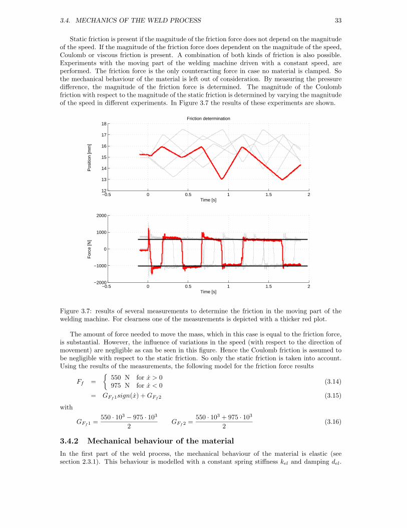
3.4. MECHANICS OF THE WELD PROCESS 33
Static friction is present if the magnitude of the friction force does not depend on the magnitudeof the speed. If the magnitude of the friction force does dependent on the magnitude of the speed,Coulomb or viscous friction is present. A combination of both kinds of friction is also possible.Experiments with the moving part of the welding machine driven with a constant speed, areperformed. The friction force is the only counteracting force in case no material is clamped. Sothe mechanical behaviour of the material is left out of consideration. By measuring the pressuredifference, the magnitude of the friction force is determined. The magnitude of the Coulombfriction with respect to the magnitude of the static friction is determined by varying the magnitudeof the speed in different experiments. In Figure 3.7 the results of these experiments are shown.
−0.5 0 0.5 1 1.5 212
13
14
15
16
17
18
Time [s]
Pos
ition
[mm
]
Friction determination
−0.5 0 0.5 1 1.5 2−2000
−1000
0
1000
2000
Time [s]
For
ce [N
]
Figure 3.7: results of several measurements to determine the friction in the moving part of thewelding machine. For clearness one of the measurements is depicted with a thicker red plot.
The amount of force needed to move the mass, which in this case is equal to the friction force,is substantial. However, the influence of variations in the speed (with respect to the direction ofmovement) are negligible as can be seen in this figure. Hence the Coulomb friction is assumed tobe negligible with respect to the static friction. So only the static friction is taken into account.Using the results of the measurements, the following model for the friction force results
Ff =
550 N for x > 0975 N for x < 0
(3.14)
= GFf 1sign(x) + GFf 2 (3.15)
with
GFf 1 =550 · 103 − 975 · 103
2GFf 2 =
550 · 103 + 975 · 103
2(3.16)
3.4.2 Mechanical behaviour of the material
In the first part of the weld process, the mechanical behaviour of the material is elastic (seesection 2.3.1). This behaviour is modelled with a constant spring stiffness kel and damping del.
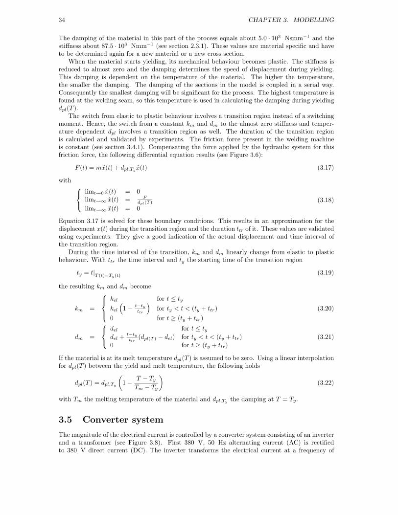
34 CHAPTER 3. MODELLING
The damping of the material in this part of the process equals about 5.0 · 103 Nsmm−1 and thestiffness about 87.5 · 103 Nmm−1 (see section 2.3.1). These values are material specific and haveto be determined again for a new material or a new cross section.
When the material starts yielding, its mechanical behaviour becomes plastic. The stiffness isreduced to almost zero and the damping determines the speed of displacement during yielding.This damping is dependent on the temperature of the material. The higher the temperature,the smaller the damping. The damping of the sections in the model is coupled in a serial way.Consequently the smallest damping will be significant for the process. The highest temperature isfound at the welding seam, so this temperature is used in calculating the damping during yieldingdpl(T ).
The switch from elastic to plastic behaviour involves a transition region instead of a switchingmoment. Hence, the switch from a constant km and dm to the almost zero stiffness and temper-ature dependent dpl involves a transition region as well. The duration of the transition regionis calculated and validated by experiments. The friction force present in the welding machineis constant (see section 3.4.1). Compensating the force applied by the hydraulic system for thisfriction force, the following differential equation results (see Figure 3.6):
F (t) = mx(t) + dpl,Tyx(t) (3.17)
with
limt→0 x(t) = 0limt→∞ x(t) = F
dpl(T )
limt→∞ x(t) = 0
(3.18)
Equation 3.17 is solved for these boundary conditions. This results in an approximation for thedisplacement x(t) during the transition region and the duration ttr of it. These values are validatedusing experiments. They give a good indication of the actual displacement and time interval ofthe transition region.
During the time interval of the transition, km and dm linearly change from elastic to plasticbehaviour. With ttr the time interval and ty the starting time of the transition region
ty = t|T (t)=Ty(t) (3.19)
the resulting km and dm become
km =
kel for t ≤ ty
kel
(
1 −t−ty
ttr
)
for ty < t < (ty + ttr)
0 for t ≥ (ty + ttr)
(3.20)
dm =
del for t ≤ tydel +
t−ty
ttr(dpl(T ) − del) for ty < t < (ty + ttr)
0 for t ≥ (ty + ttr)
(3.21)
If the material is at its melt temperature dpl(T ) is assumed to be zero. Using a linear interpolationfor dpl(T ) between the yield and melt temperature, the following holds
dpl(T ) = dpl,Ty
(
1 −T − Ty
Tm − Ty
)
(3.22)
with Tm the melting temperature of the material and dpl,Tythe damping at T = Ty.
3.5 Converter system
The magnitude of the electrical current is controlled by a converter system consisting of an inverterand a transformer (see Figure 3.8). First 380 V, 50 Hz alternating current (AC) is rectifiedto 380 V direct current (DC). The inverter transforms the electrical current at a frequency of

3.6. HYDRAULIC SYSTEM 35
1000 Hz by means of pulswidth modulation. The transformer and rectifier transform the resultingpower to 0 to 60 kA DC at a voltage of 0 to 10 V.
The output of the inverter is controlled by a built-in current controller. The controller uses theoutput current of the inverter and the resulting measured output current of the transformer. In thisway the electrical current resulting from the converter system can be controlled in between 0 and60 kA DC. The control signal of the inverter can be varied in a range of 0 to 1 V, correspondingto this 0 and 60 kA. During this study a maximum of 40 kA instead of 60 kA is used due to amalfunction of the inverter.
Control
rectifier with direct current link circuit and transistor inverterwelding transformer
and rectifier
Currentmeasurement
380V, AC50Hz
0-10V, DC0-60kA
Figure 3.8: schematic overview of the converter system.
Trials to identify the closed loop converter system with the built-in current controller wereperformed. However this appeared to be hard, so the manufacturer’s specifications are used tomodel this system. Although deficient, the measurement results indicated a bandwidth of 1000 Hz,which corresponds to the specifications. The range of the transformer is 0 to 40 kA, so a 2ndorderhigh frequent filter with a gain Gcs = 40 · 103 is used
ωcs,o = 1000 Hz (3.23)
ξcs = 0.6 (3.24)
with ωcs,o and ξcs the natural frequency respectively the damping of the 2ndorder filter.
3.6 Hydraulic system
The hydraulic system is an important part of the setup. The upset force as well as the displacementin the process can be controlled by steering the input signal of the servo valve. Various calculations,measurements and modelling of the hydraulic system have been performed in previous studies.However none resulted in a model good enough to use as a reliable representation of the hydraulicsystem or the developed models could not be validated because of a lack of good measurements.The controller used at the moment suffices for the purpose it is used for. But because it is partlybased on trial and error instead of on theoretical base, the possibilities of the hydraulic systemare not utilised to its full potential. Consequently special attention is paid to the modelling andthe control of the hydraulic system in this study.
To start with, an overview of hydraulic system is given. Next a parametric white box model ofthe hydraulic system is developed. This model is linearised so that the results can be verified usingthe frequency domain. Apart from this model a black box model is fitted, based on measurementsperformed on the hydraulic system at the setup. These results are also evaluated using thefrequency domain. Next the results of the black box model, of the white box model and of the
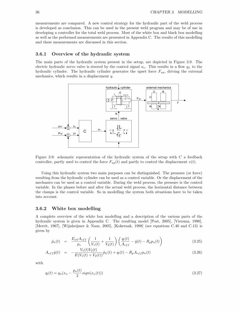
36 CHAPTER 3. MODELLING
measurements are compared. A new control strategy for the hydraulic part of the weld processis developed as conclusion. This can be used in the present weld program and may be of use indeveloping a controller for the total weld process. Most of the white box and black box modellingas well as the performed measurements are presented in Appendix C. The results of this modellingand these measurements are discussed in this section.
3.6.1 Overview of the hydraulic system
The main parts of the hydraulic system present in the setup, are depicted in Figure 3.9. Theelectric hydraulic servo valve is steered by the control signal uv. This results in a flow qL to thehydraulic cylinder. The hydraulic cylinder generates the upset force Fup, driving the externalmechanics, which results in a displacement y.
Cuv
qL
SPref
eyyrefS
eP
Fup
y
external mechanicshydraulic cylinder
servo valve
y(t)
Aeff
Q *(t)inQ (t)outQ *(t)out Q (t)in
1 2d
dpdpr
piston rod
F(t)
Figure 3.9: schematic representation of the hydraulic system of the setup with C a feedbackcontroller, partly used to control the force Fup(t) and partly to control the displacement x(t).
Using this hydraulic system two main purposes can be distinguished. The pressure (or force)resulting from the hydraulic cylinder can be used as a control variable. Or the displacement of themechanics can be used as a control variable. During the weld process, the pressure is the controlvariable. In the phases before and after the actual weld process, the horizontal distance betweenthe clamps is the control variable. So in modelling the system both situations have to be takeninto account.
3.6.2 White box modelling
A complete overview of the white box modelling and a description of the various parts of thehydraulic system is given in Appendix C. The resulting model [Post, 2005], [Viersma, 1990],[Merrit, 1967], [Wijnheijmer & Naus, 2005], [Kokernak, 1998] (see equations C.40 and C.13) isgiven by
pn(t) =EoilAeff
ps
(
1
V1(t)+
1
V2(t)
)(
ql(t)
Aeff
− y(t) − Rppn(t)
)
(3.25)
Aeff y(t) = −V1(t)V2(t)
E(V1(t) + V2(t))pL(t) + ql(t) − RpAeffpn(t) (3.26)
with
ql(t) = qn(xn −pn(t)
2sign(xn(t))) (3.27)

3.6. HYDRAULIC SYSTEM 37
Both the electric hydraulic servo valve and the hydraulic actuator show nonlinear behaviour(see equations 3.25 to 3.27). The nonlinear, time domain models of the servo valve and hydrauliccylinder are linearised and transformed to the frequency domain. In this way insight in thecharacteristics of the hydraulic system is expanded. Moreover, validation of the model usingmeasurement data, becomes easier. The natural frequency of the hydraulic cylinder with coupledmass, is dependent on the position of the rod y(t) (see equations 3.25 and 3.26). If the rod is onhalf of the stroke of the cylinder (at mid stroke), the natural frequency becomes minimal. Thehydraulic stiffness of the hydraulic cylinder equals
Co(t) = EoilA2eff
(
1
V1(t)+
1
V2(t)
)
(3.28)
=EoilAeffLL2
4 − y(t)2(3.29)
with y(t) defined as a displacement from mid stroke. So the theoretical natural frequency of thehydraulic cylinder equals
ωo =
√
Co(t)
m(3.30)
Only the influence of the position of the rod on the natural frequency is shown. Validation usingmeasurements is discussed in the next section. In Figure 3.10 the pressure transfer function of thehydraulic system is shown at three different positions of the rod. The positions are y = 0 mm,y = 10 mm and y = 13 mm. From equations 3.29 and 3.30 the theoretical natural frequencyof the hydraulic cylinder can be calculated. For these positions, this natural frequency equals95 Hz, 129 Hz respectively 192 Hz. Figure 3.10 shows that the results of the white box modelcorrespond well to these values.
101
102
103
−60
−40
−20
0
20
40Pressure transfer function of the white box model of the hydraulic system
Am
plitu
de [d
B]
101
102
103
−300
−200
−100
0
100
Frequency [Hz]
Pha
se [d
egre
es]
Figure 3.10: pressure transfer functions of the hydraulic system resulting from the white boxmodel at various rod positions y.

38 CHAPTER 3. MODELLING
3.6.3 Measurements and black box modelling
The techniques described in section C.2 of Appendix C are used to determine the transfer functionsof the hydraulic servo system of the setup. The pressure as well as the displacement resulting fromthe hydraulic system are of importance in the weld process. So two distinctive transfer functionsare determined. The transfer function estimates of the pressure and of the displacement areshown in Figure 3.11. The measurements at the setup to determine these transfer functions, areperformed with the rod positioned at mid stroke. Using CDesign [MCDesign, 2005] a black boxmodel is fitted over the measurement results (see also Figure 3.11). In fitting the black box model,the restrictions determined in section C.3 of Appendix C are taken into account. This black boxmodel is off course only valid for this rod position. The transfer functions resulting from thelinearised white box model are show in Figure 3.11 as well. A mechanical model of the weldingmachine including its mass and static friction is used as external mechanics in the white boxmodel. This mechanical model is discussed in more detail in section 3.4 and section C.1.3.
101
102
−40
−30
−20
−10
0
10Pressure transfer function of the hydraulic system
Mag
nitu
de [d
B]
101
102
−400
−300
−200
−100
0
100
200
Frequency [Hz]
Pha
se [d
egre
es]
(a) pressure transfer function
101
102
−120
−100
−80
−60
−40
−20
0Pressure transfer function of the hydraulic system
Mag
nitu
de [d
B]
101
102
−500
−400
−300
−200
−100
0
Frequency [Hz]
Pha
se [d
egre
es]
(b) position transfer function
Figure 3.11: transfer functions of the white box model (the dashed red plots), resulting frommeasurements (the blue plots), and the black box model (the (light) green plots on top of theothers). (a): transfer function of the pressure. (b): transfer functions of the position.
Because the measurements are performed with the rod positioned at mid stoke, the transferfunction estimates of these measurements show the lowest natural frequency of the system. Thelower the natural frequency, the smaller the bandwidth of the system will be. Consequently,the working point with the lowest natural frequency has to be used in modelling, consideringrobustness of the controlled system. In this way, the developed controllers will be robust for otherworking points as well. Hence the fitted black box model is used in further development of anew controller for the hydraulic system (see section 3.6.4). Because of the position dependentcharacteristics, the white box model is used in further modelling of the total weld process.
3.6.4 Control of the hydraulic system
The hydraulic system is used to control the position of the rod as well as the welding force. Duringthe weld process, the upset force has to be controlled. Before and after the actual weld process,the system is position controlled. The design of a position controller is not further discussed atthis point. More details on the control of the position can be found in Wijnheijmer & Naus [2005].In Figure 3.12(a) the characteristic progress of the demanded force and of the actual force during aweld process are depicted. The controller used, is the present force controller of WELD2001. Thiscontroller is dependent on the speed of displacement. In Figure 3.13, the controllers corresponding

3.7. MODELLING RESULTS 39
0 0.2 0.4 0.6 0.8 1 1.2 1.4 1.6 1.8 20
2
4
6
8
10
12
14
16
Time [s]
For
ce [k
N]
Pressure development using the controller of WELD2001
(a) old control
0 0.2 0.4 0.6 0.8 1 1.2 1.4 1.6 1.8 20
2
4
6
8
10
12
14
16
Time [s]
For
ce [k
N]
Pressure development using a new controller
(b) new control
Figure 3.12: (a): the old control of the force in the weld process and a (b) new controller. Thedotted plot indicates the setpoint signal and the solid plot the actual force.
to a speed of 0 mms−1 and of 15 mms−1 are shown. In the yielding phase, an extra boost inthe reference trajectory of the force is present. This boost is prescribed to overcome the suddendrop in compression at the welding seam. Its purpose is not to increase the force, but to keep itrelatively constant, which, as can be seen in Figure 3.12(a), is the case. At the end of the boost,nothing is left of it in the actual force. Consequently a new controller is developed apart from thestudy to a new control strategy for the total weld process. The fitted black box models are usedto apply loop shaping techniques using CDesign [MCDesign, 2005]. The developed controller isshown in Figure 3.13. A clear distinction between the present controllers and the new controllercan be noticed. The new controller damps the natural frequency of the system, where the oldcontrollers only have an integrating action. In this way, the bandwidth of the controlled systemcan be increased. In Figure 3.12(b), a simulation result using the newly designed controller isshown. Comparing this figure to Figure 3.12(a) indicates the adequacy of the new controller.
3.7 Modelling results
All modelled parts of the weld process, as discussed before, are now combined to a single model.This results in a complete model, which can be used to simulate the weld process off-line, seeSimulationModel.mdl in Appendix F. The model is developed using Simulink. To facilitateworking with this model, a Simulink Library is written, see Appendix B. Models of the hydraulicsystem and of the converter system are already validated separately (see sections 3.5 and 3.6). Sothe main attention in this section lies on the results of the weld process part, the thermodynamicaland mechanical parts of the model. The progress of the electrical current, of the pressure and ofthe displacement are measured during the weld process. These measurement results are comparedto the results of simulations to test the validity of the model. The progress of the modelled pressureand electrical current follow from the combination of the weld program and the hydraulic systemrespectively the converter system. So the displacement is the only variable that can be used tovalidate these parts directly. The temperature is an important variable in the weld process too,but it is not measured. However, some experiments using thermocouples and an infrared cameraare performed. In this way an indication of the real temperature progress during the weld processis obtained. The results of these experiments are compared to the temperature progress resultingfrom the model. In Figures 3.14 and 3.15 the results of several experiments with varying magnitudeof the electrical current and of the force are compared to the results of simulations. The simulation

40 CHAPTER 3. MODELLING
100
101
102
103
104
−10
0
10
20
30Transfer functions of the present and new force controllers
Mag
nitu
de [d
B]
100
101
102
103
104
−200
−150
−100
−50
0
50
100
Pha
se [d
egre
es]
Frequency [Hz]
Figure 3.13: the force feedback controllers of the hydraulic system as implemented in WELD2001(the solid red and green plots) and a newly designed controller based on the black box model (thedashed blue plot).
model used for these experiments did not include the models of the hydraulic system and convertersystem yet. Hence, the setpoints for these variables are used instead of the controlled variables.The weld programs used in the simulations are the same as those used in the experiments.
The switching moments between the various phases can be determined from the progress of theelectrical current and of the force. They correspond good as can be seen in Figures 3.14 and 3.15.The amplitude of the displacement progress of the model also corresponds well to the experiments.So from these results, it may be concluded that the thermodynamical and mechanical part of theweld process are modelled well enough to provide a good representation of the progress of thedisplacement during the actual weld process.
The displacement progress is dependent on both the thermodynamics and mechanics of theprocess. Consequently the temperature progress resulting from the model is assumed to give agood indication of the real temperature progress. In Figure 3.16 the results of measurements usinga thermo couple and an infrared camera are compared to the temperature progress resulting fromsimulations. A comment on these measurements is that both measurements are random samplesinstead of results of a series of tests. Consequently, the weld programs of Figure 3.16(a) and3.16(b) differ. Besides, the measurements give an indication of the temperature at a single pointin the welding seam. The temperature values resulting from the simulations however, representan average temperature over the welding seam. From the results can be concluded that the timeintervals of the heating and of the yielding are comparable. The same applies for the maximumtemperature reached during the process. The actual progress of the temperature however can bebetter registered by the measurements of the infrared camera. The temperature progress duringcooling down is better represented by the thermo couple measurement. So an indication of thetemperature resulting from the simulation model is given. But no unambiguous conclusions canbe drawn concerning the validity of this progress with respect to the performed measurements.
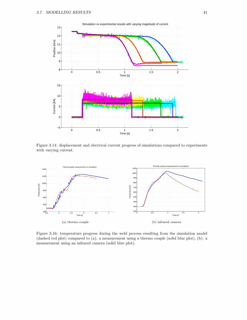
3.7. MODELLING RESULTS 41
0 0.5 1 1.5 28
9
10
11
12
13
Time [s]
Pos
ition
[mm
]
Simulation vs experimental results with varying magnitude of current
0 0.5 1 1.5 2−5
0
5
10
15
Time [s]
Cur
rent
[kA
]
Figure 3.14: displacement and electrical current progress of simulations compared to experimentswith varying current.
4.5 5 5.5 6 6.5 7200
400
600
800
1000
1200
1400Thermocouple measurement vs simulation
Time [s]
Tem
pera
ture
[K]
(a) thermo couple
0 0.5 1 1.5 2200
300
400
500
600
700
800
900
1000
1100Thermal camera measurement vs simulation
Time [s]
Tem
pera
ture
[K]
(b) infrared camera
Figure 3.16: temperature progress during the weld process resulting from the simulation model(dashed red plot) compared to (a): a measurement using a thermo couple (solid blue plot), (b): ameasurement using an infrared camera (solid blue plot).
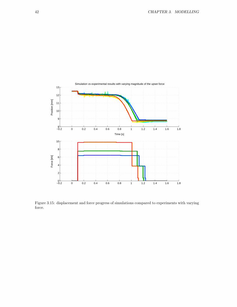
42 CHAPTER 3. MODELLING
−0.2 0 0.2 0.4 0.6 0.8 1 1.2 1.4 1.6 1.88
9
10
11
12
13
Time [s]
Pos
ition
[mm
]
Simulation vs experimental results with varying magnitude of the upset force
−0.2 0 0.2 0.4 0.6 0.8 1 1.2 1.4 1.6 1.80
2
4
6
8
10
Time [s]
For
ce [k
N]
Figure 3.15: displacement and force progress of simulations compared to experiments with varyingforce.

Chapter 4
Control
The aim of this study is to develop a more robust and reliable control strategy based on goodinsight in the weld process. The development of the controller is presented in this chapter. Firstthe demands to the controller and the possible control strategies to apply, are discussed. Fromthis a new control strategy, including an on-line temperature calculation, reference trajectoriesand the actual controller design, follows. Finally the implementation of the controller and theresults are discussed.
4.1 Demands to the controller
The demands to the new control strategy are derived mainly from the advantages and disad-vantages of the present control strategy. The present control of the weld process is based on adiscrete steering of the force and electrical current. The process is divided into 5 phases based onposition and time restrictions. Consequently the position is a restriction, limiting the amount ofdisplacement per phase instead of really prescribing the position progress during the weld process.Most of the welding machines are part of an automated rim production line and thus only havea predefined amount of time to perform the weld process. Moreover, the weld process often isone of the time restricting processes (see section 1.3). The time the process takes however, isonly limited per phase. So the process time is not predefined and can only be tuned via trial anderror. Consequently the magnitude of the electrical current and the force are based on trial anderror instead of being dependent on material parameters. Setting these variables during switchingbetween different materials or rim sizes takes a lot of time and experience. The quality of theweld depends on the resulting christalline structure of the material in the weld. This structure inparticular depends on the temperature progress of the material during welding. As this tempera-ture is not measured nor coupled to the weld program, nothing can be said about the weld qualitywith respect to the weld program. The most important demands to the controller thus are:
• a reproducible weld process
• execution of the weld process within a previously defined time interval
• the demanded amount of upset has to be reached exactly
• if possible, some control of the temperature is desirable. In this way the resulting crystallinestructure of the material of the weld may be influenced.
Apart from these demands, practical advantages for the customer are also of importance. Failureof rims by cracking seems to happen arbitrarily at the moment. If the weld process is controlled
43
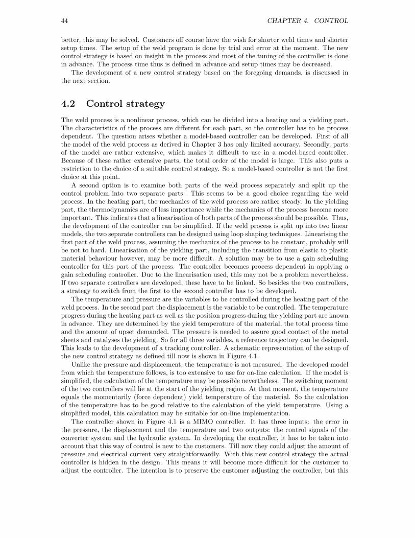
44 CHAPTER 4. CONTROL
better, this may be solved. Customers off course have the wish for shorter weld times and shortersetup times. The setup of the weld program is done by trial and error at the moment. The newcontrol strategy is based on insight in the process and most of the tuning of the controller is donein advance. The process time thus is defined in advance and setup times may be decreased.
The development of a new control strategy based on the foregoing demands, is discussed inthe next section.
4.2 Control strategy
The weld process is a nonlinear process, which can be divided into a heating and a yielding part.The characteristics of the process are different for each part, so the controller has to be processdependent. The question arises whether a model-based controller can be developed. First of allthe model of the weld process as derived in Chapter 3 has only limited accuracy. Secondly, partsof the model are rather extensive, which makes it difficult to use in a model-based controller.Because of these rather extensive parts, the total order of the model is large. This also puts arestriction to the choice of a suitable control strategy. So a model-based controller is not the firstchoice at this point.
A second option is to examine both parts of the weld process separately and split up thecontrol problem into two separate parts. This seems to be a good choice regarding the weldprocess. In the heating part, the mechanics of the weld process are rather steady. In the yieldingpart, the thermodynamics are of less importance while the mechanics of the process become moreimportant. This indicates that a linearisation of both parts of the process should be possible. Thus,the development of the controller can be simplified. If the weld process is split up into two linearmodels, the two separate controllers can be designed using loop shaping techniques. Linearising thefirst part of the weld process, assuming the mechanics of the process to be constant, probably willbe not to hard. Linearisation of the yielding part, including the transition from elastic to plasticmaterial behaviour however, may be more difficult. A solution may be to use a gain schedulingcontroller for this part of the process. The controller becomes process dependent in applying again scheduling controller. Due to the linearisation used, this may not be a problem nevertheless.If two separate controllers are developed, these have to be linked. So besides the two controllers,a strategy to switch from the first to the second controller has to be developed.
The temperature and pressure are the variables to be controlled during the heating part of theweld process. In the second part the displacement is the variable to be controlled. The temperatureprogress during the heating part as well as the position progress during the yielding part are knownin advance. They are determined by the yield temperature of the material, the total process timeand the amount of upset demanded. The pressure is needed to assure good contact of the metalsheets and catalyses the yielding. So for all three variables, a reference trajectory can be designed.This leads to the development of a tracking controller. A schematic representation of the setup ofthe new control strategy as defined till now is shown in Figure 4.1.
Unlike the pressure and displacement, the temperature is not measured. The developed modelfrom which the temperature follows, is too extensive to use for on-line calculation. If the model issimplified, the calculation of the temperature may be possible nevertheless. The switching momentof the two controllers will lie at the start of the yielding region. At that moment, the temperatureequals the momentarily (force dependent) yield temperature of the material. So the calculationof the temperature has to be good relative to the calculation of the yield temperature. Using asimplified model, this calculation may be suitable for on-line implementation.
The controller shown in Figure 4.1 is a MIMO controller. It has three inputs: the error inthe pressure, the displacement and the temperature and two outputs: the control signals of theconverter system and the hydraulic system. In developing the controller, it has to be taken intoaccount that this way of control is new to the customers. Till now they could adjust the amount ofpressure and electrical current very straightforwardly. With this new control strategy the actualcontroller is hidden in the design. This means it will become more difficult for the customer toadjust the controller. The intention is to preserve the customer adjusting the controller, but this
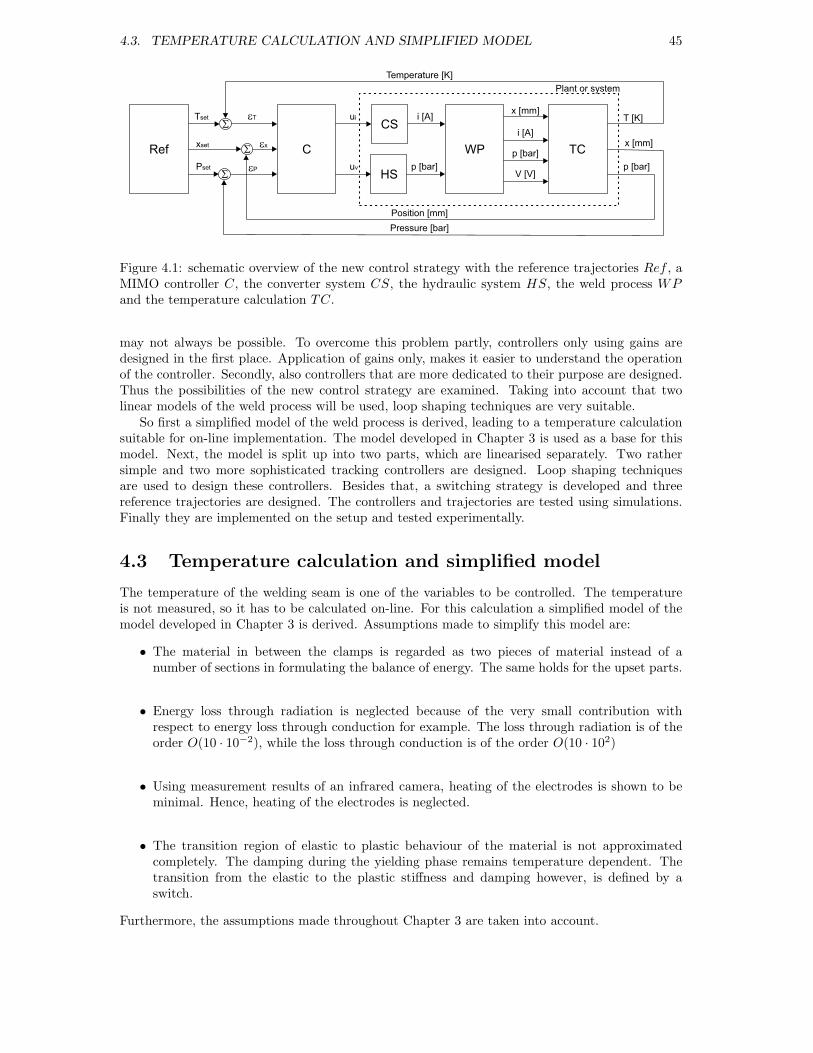
4.3. TEMPERATURE CALCULATION AND SIMPLIFIED MODEL 45
Ref C
CS
HS
WP TC
S
S
S
x [mm]
i [A]
p [bar]
V [V]
i [A]
p [bar]
ui
uveP
ex
eTTset
Pset
xset
Temperature [K]
Position [mm]
Pressure [bar]
Plant or system
x [mm]
p [bar]
T [K]
Figure 4.1: schematic overview of the new control strategy with the reference trajectories Ref , aMIMO controller C, the converter system CS, the hydraulic system HS, the weld process WPand the temperature calculation TC.
may not always be possible. To overcome this problem partly, controllers only using gains aredesigned in the first place. Application of gains only, makes it easier to understand the operationof the controller. Secondly, also controllers that are more dedicated to their purpose are designed.Thus the possibilities of the new control strategy are examined. Taking into account that twolinear models of the weld process will be used, loop shaping techniques are very suitable.
So first a simplified model of the weld process is derived, leading to a temperature calculationsuitable for on-line implementation. The model developed in Chapter 3 is used as a base for thismodel. Next, the model is split up into two parts, which are linearised separately. Two rathersimple and two more sophisticated tracking controllers are designed. Loop shaping techniquesare used to design these controllers. Besides that, a switching strategy is developed and threereference trajectories are designed. The controllers and trajectories are tested using simulations.Finally they are implemented on the setup and tested experimentally.
4.3 Temperature calculation and simplified model
The temperature of the welding seam is one of the variables to be controlled. The temperatureis not measured, so it has to be calculated on-line. For this calculation a simplified model of themodel developed in Chapter 3 is derived. Assumptions made to simplify this model are:
• The material in between the clamps is regarded as two pieces of material instead of anumber of sections in formulating the balance of energy. The same holds for the upset parts.
• Energy loss through radiation is neglected because of the very small contribution withrespect to energy loss through conduction for example. The loss through radiation is of theorder O(10 · 10−2), while the loss through conduction is of the order O(10 · 102)
• Using measurement results of an infrared camera, heating of the electrodes is shown to beminimal. Hence, heating of the electrodes is neglected.
• The transition region of elastic to plastic behaviour of the material is not approximatedcompletely. The damping during the yielding phase remains temperature dependent. Thetransition from the elastic to the plastic stiffness and damping however, is defined by aswitch.
Furthermore, the assumptions made throughout Chapter 3 are taken into account.

46 CHAPTER 4. CONTROL
Defining the state vector x(t)
x(t) =
x1 = normalised spool valve position xn(t)x2 = velocity of the normalised spool valve movement xn(t)x3 = normalised pressure pn(t)x4 = welding seam temperature T (t)x5 = displacement of the right clamp y(t)x6 = velocity of the right clamp y(t)x7 = electrical current i(t)
x8 = time derivative of the electrical current i(t)
(4.1)
the input vector u(t)
u(t) =
[
u1 = inverter control signal ui(t)u2 = servo valve control signal uv(t)
]
(4.2)
and the output vector y(t)
y(t) =
y1 = displacement y(t)y2 = temperature T (t)y3 = normalised pressure pn(t)
(4.3)
the nonlinear state-space representation of the model becomes
x(t) = f(x(t), u(t)) (4.4)
y(t) = g(x(t), u(t))
An overview of the resulting set of nonlinear differential equations f(x(t), u(t)) and g(x(t), u(t))is given in Appendix D.
The temperature progress influences the quality of the resulting weld. Consequently the tem-perature calculation has be a good approximation of the real temperature progress during theweld process. As far as good control is considered however, it should be a good fit with respectto the calculation of the yield temperature. The yield temperature of the material is dependenton the upset force and the characteristic yield stress at room temperature (see equation 2.5). Theyield temperature is calculated on-line as well. It defines the switch from the heating phase to theyielding phase and consequently a switch in control strategy.
The model derived in Chapter 3 was validated by the progress of the displacement (see section3.7). Taking into account the assumptions made at the start of this section, this is not possiblefor this simplified model. The progress of the displacement is used as the main validation variablein section 3.7. The transition region is not taken into account in this simplified model, so theprogress of the displacement is not representative. However, the calculation of the temperaturewith respect to the calculation of the yield temperature can be validated. The switch from elasticto plastic material behaviour is defined by reaching the yield temperature. This moment in theweld process is calculated by the model and can be determined from the measured pressure orposition progress as well. Experimental results show that the simplified and the temperaturecalculation meet their purpose.
The temperature progress resulting from a simulation is compared to the measurement as usedin Figure 3.16(b) (see Figure 4.2). The progress of the temperature while heating the material isthe main goal of this model. Hence, the measurement using a thermo couple (see Figure 3.16(a))is not used in this case. The temperature progress resulting from the model reaches the samemaximum value as the measured temperature. The amount of time the total heating takes is alsocomparable.
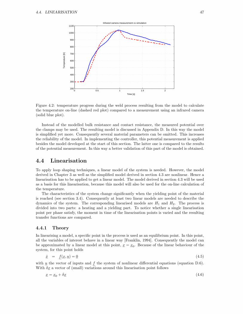
4.4. LINEARISATION 47
0 0.5 1 1.5 2200
300
400
500
600
700
800
900
1000
1100Infrared camera measurement vs simulation
Time [s]
Tem
pera
ture
[K]
Figure 4.2: temperature progress during the weld process resulting from the model to calculatethe temperature on-line (dashed red plot) compared to a measurement using an infrared camera(solid blue plot).
Instead of the modelled bulk resistance and contact resistance, the measured potential overthe clamps may be used. The resulting model is discussed in Appendix D. In this way the modelis simplified yet more. Consequently several material parameters can be omitted. This increasesthe reliability of the model. In implementing the controller, this potential measurement is appliedbesides the model developed at the start of this section. The latter one is compared to the resultsof the potential measurement. In this way a better validation of this part of the model is obtained.
4.4 Linearisation
To apply loop shaping techniques, a linear model of the system is needed. However, the modelderived in Chapter 3 as well as the simplified model derived in section 4.3 are nonlinear. Hence alinearisation has to be applied to get a linear model. The model derived in section 4.3 will be usedas a basis for this linearisation, because this model will also be used for the on-line calculation ofthe temperature.
The characteristics of the system change significantly when the yielding point of the materialis reached (see section 3.4). Consequently at least two linear models are needed to describe thedynamics of the system. The corresponding linearised models are H1 and H2. The process isdivided into two parts: a heating and a yielding part. To notice whether a single linearisationpoint per phase satisfy, the moment in time of the linearisation points is varied and the resultingtransfer functions are compared.
4.4.1 Theory
In linearising a model, a specific point in the process is used as an equilibrium point. In this point,all the variables of interest behave in a linear way [Franklin, 1994]. Consequently the model canbe approximated by a linear model at this point, x = x0. Because of the linear behaviour of thesystem, for this point holds
x = f(x, u) = 0 (4.5)
with u the vector of inputs and f the system of nonlinear differential equations (equation D.6).With δx a vector of (small) variations around this linearisation point follows
x = x0 + δx (4.6)
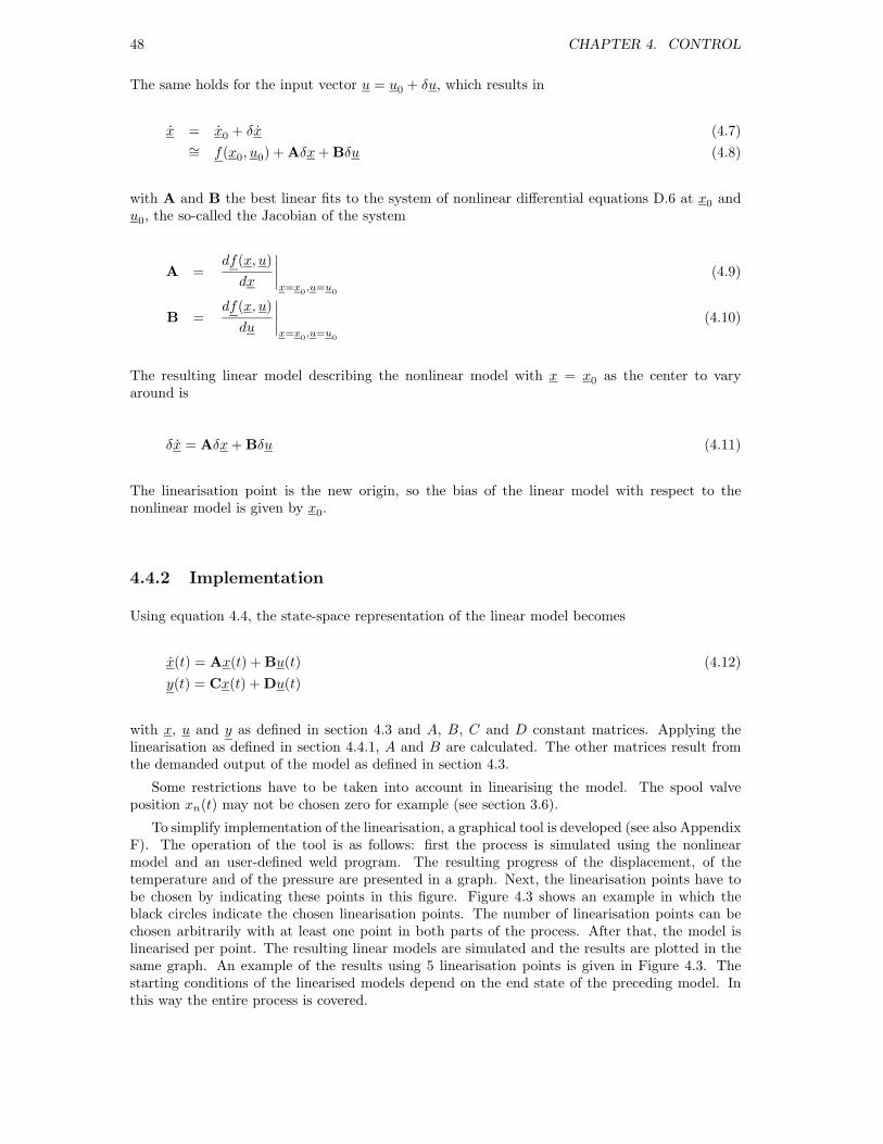
48 CHAPTER 4. CONTROL
The same holds for the input vector u = u0 + δu, which results in
x = x0 + δx (4.7)∼= f(x0, u0) + Aδx + Bδu (4.8)
with A and B the best linear fits to the system of nonlinear differential equations D.6 at x0 andu0, the so-called the Jacobian of the system
A =df(x, u)
dx
∣
∣
∣
∣
x=x0,u=u
0
(4.9)
B =df(x, u)
du
∣
∣
∣
∣
x=x0,u=u
0
(4.10)
The resulting linear model describing the nonlinear model with x = x0 as the center to varyaround is
δx = Aδx + Bδu (4.11)
The linearisation point is the new origin, so the bias of the linear model with respect to thenonlinear model is given by x0.
4.4.2 Implementation
Using equation 4.4, the state-space representation of the linear model becomes
x(t) = Ax(t) + Bu(t) (4.12)
y(t) = Cx(t) + Du(t)
with x, u and y as defined in section 4.3 and A, B, C and D constant matrices. Applying thelinearisation as defined in section 4.4.1, A and B are calculated. The other matrices result fromthe demanded output of the model as defined in section 4.3.
Some restrictions have to be taken into account in linearising the model. The spool valveposition xn(t) may not be chosen zero for example (see section 3.6).
To simplify implementation of the linearisation, a graphical tool is developed (see also AppendixF). The operation of the tool is as follows: first the process is simulated using the nonlinearmodel and an user-defined weld program. The resulting progress of the displacement, of thetemperature and of the pressure are presented in a graph. Next, the linearisation points have tobe chosen by indicating these points in this figure. Figure 4.3 shows an example in which theblack circles indicate the chosen linearisation points. The number of linearisation points can bechosen arbitrarily with at least one point in both parts of the process. After that, the model islinearised per point. The resulting linear models are simulated and the results are plotted in thesame graph. An example of the results using 5 linearisation points is given in Figure 4.3. Thestarting conditions of the linearised models depend on the end state of the preceding model. Inthis way the entire process is covered.
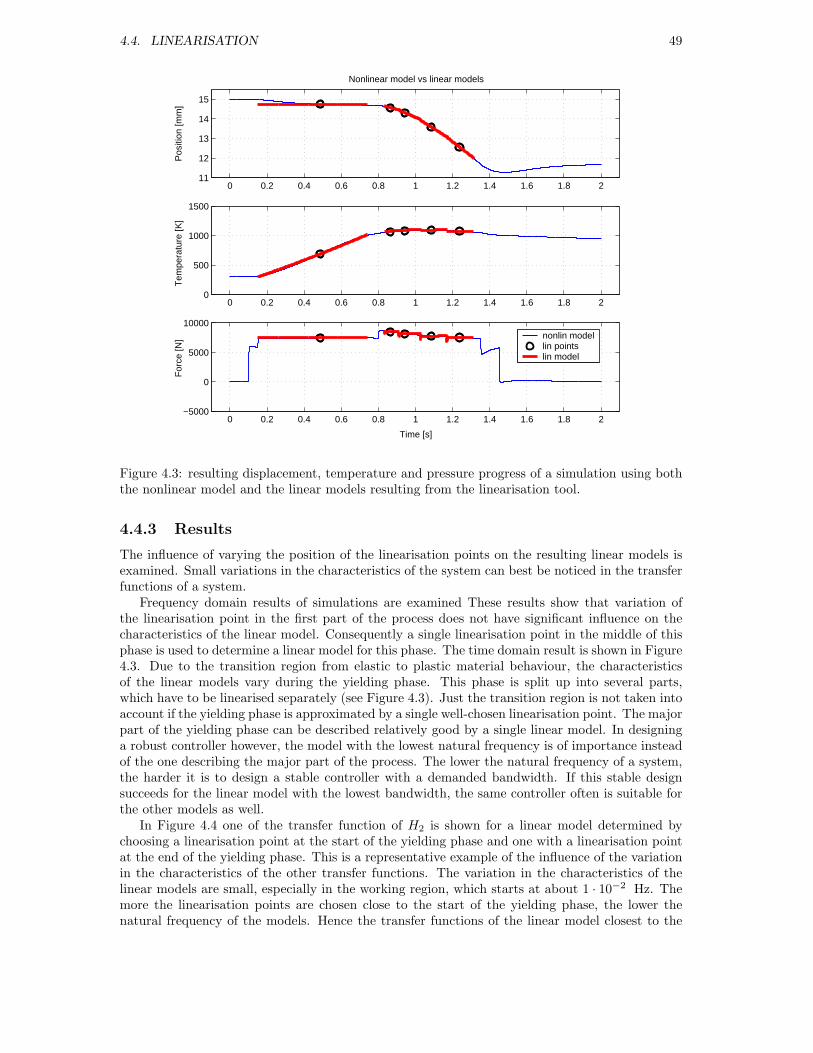
4.4. LINEARISATION 49
0 0.2 0.4 0.6 0.8 1 1.2 1.4 1.6 1.8 211
12
13
14
15
Pos
ition
[mm
]
Nonlinear model vs linear models
0 0.2 0.4 0.6 0.8 1 1.2 1.4 1.6 1.8 20
500
1000
1500
Tem
pera
ture
[K]
0 0.2 0.4 0.6 0.8 1 1.2 1.4 1.6 1.8 2−5000
0
5000
10000
For
ce [N
]
Time [s]
nonlin modellin pointslin model
Figure 4.3: resulting displacement, temperature and pressure progress of a simulation using boththe nonlinear model and the linear models resulting from the linearisation tool.
4.4.3 Results
The influence of varying the position of the linearisation points on the resulting linear models isexamined. Small variations in the characteristics of the system can best be noticed in the transferfunctions of a system.
Frequency domain results of simulations are examined These results show that variation ofthe linearisation point in the first part of the process does not have significant influence on thecharacteristics of the linear model. Consequently a single linearisation point in the middle of thisphase is used to determine a linear model for this phase. The time domain result is shown in Figure4.3. Due to the transition region from elastic to plastic material behaviour, the characteristicsof the linear models vary during the yielding phase. This phase is split up into several parts,which have to be linearised separately (see Figure 4.3). Just the transition region is not taken intoaccount if the yielding phase is approximated by a single well-chosen linearisation point. The majorpart of the yielding phase can be described relatively good by a single linear model. In designinga robust controller however, the model with the lowest natural frequency is of importance insteadof the one describing the major part of the process. The lower the natural frequency of a system,the harder it is to design a stable controller with a demanded bandwidth. If this stable designsucceeds for the linear model with the lowest bandwidth, the same controller often is suitable forthe other models as well.
In Figure 4.4 one of the transfer function of H2 is shown for a linear model determined bychoosing a linearisation point at the start of the yielding phase and one with a linearisation pointat the end of the yielding phase. This is a representative example of the influence of the variationin the characteristics of the other transfer functions. The variation in the characteristics of thelinear models are small, especially in the working region, which starts at about 1 · 10−2 Hz. Themore the linearisation points are chosen close to the start of the yielding phase, the lower thenatural frequency of the models. Hence the transfer functions of the linear model closest to the
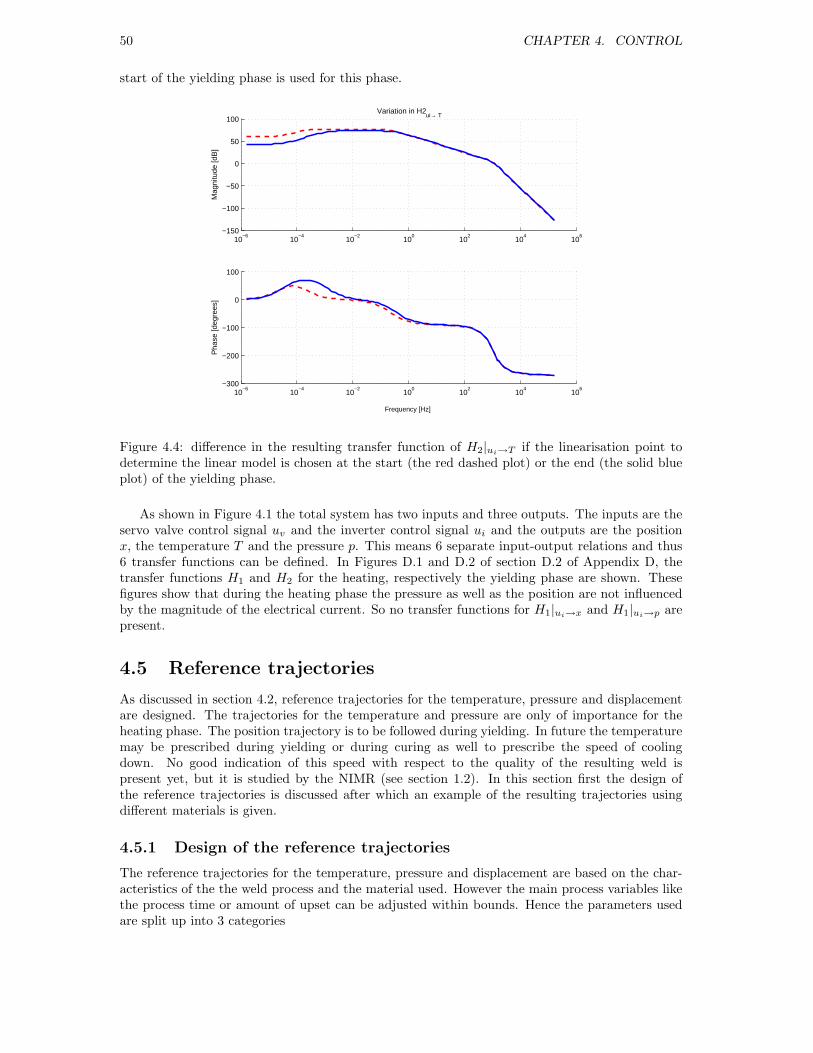
50 CHAPTER 4. CONTROL
start of the yielding phase is used for this phase.
10−6
10−4
10−2
100
102
104
106
−150
−100
−50
0
50
100
Mag
nitu
de [d
B]
Variation in H2ui→ T
10−6
10−4
10−2
100
102
104
106
−300
−200
−100
0
100
Pha
se [d
egre
es]
Frequency [Hz]
Figure 4.4: difference in the resulting transfer function of H2|ui→T if the linearisation point todetermine the linear model is chosen at the start (the red dashed plot) or the end (the solid blueplot) of the yielding phase.
As shown in Figure 4.1 the total system has two inputs and three outputs. The inputs are theservo valve control signal uv and the inverter control signal ui and the outputs are the positionx, the temperature T and the pressure p. This means 6 separate input-output relations and thus6 transfer functions can be defined. In Figures D.1 and D.2 of section D.2 of Appendix D, thetransfer functions H1 and H2 for the heating, respectively the yielding phase are shown. Thesefigures show that during the heating phase the pressure as well as the position are not influencedby the magnitude of the electrical current. So no transfer functions for H1|ui→x and H1|ui→p arepresent.
4.5 Reference trajectories
As discussed in section 4.2, reference trajectories for the temperature, pressure and displacementare designed. The trajectories for the temperature and pressure are only of importance for theheating phase. The position trajectory is to be followed during yielding. In future the temperaturemay be prescribed during yielding or during curing as well to prescribe the speed of coolingdown. No good indication of this speed with respect to the quality of the resulting weld ispresent yet, but it is studied by the NIMR (see section 1.2). In this section first the design ofthe reference trajectories is discussed after which an example of the resulting trajectories usingdifferent materials is given.
4.5.1 Design of the reference trajectories
The reference trajectories for the temperature, pressure and displacement are based on the char-acteristics of the the weld process and the material used. However the main process variables likethe process time or amount of upset can be adjusted within bounds. Hence the parameters usedare split up into 3 categories
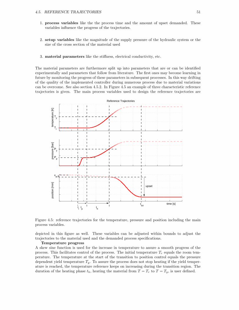
4.5. REFERENCE TRAJECTORIES 51
1. process variables like the the process time and the amount of upset demanded. Thesevariables influence the progress of the trajectories.
2. setup variables like the magnitude of the supply pressure of the hydraulic system or thesize of the cross section of the material used
3. material parameters like the stiffness, electrical conductivity, etc.
The material parameters are furthermore split up into parameters that are or can be identifiedexperimentally and parameters that follow from literature. The first ones may become learning infuture by monitoring the progress of these parameters in subsequent processes. In this way driftingof the quality of the implemented controller during numerous process due to material variationscan be overcome. See also section 4.5.2. In Figure 4.5 an example of three characteristic referencetrajectories is given. The main process variables used to design the reference trajectories are
posi
tion
[mm
]
time [s]
upset
xel
tp
th
ttot
ti
tem
pera
ture
[K]
Reference Trajectories
Ty
Tr
pres
sure
[bar
]
Pp
Py
Figure 4.5: reference trajectories for the temperature, pressure and position including the mainprocess variables.
depicted in this figure as well. These variables can be adjusted within bounds to adjust thetrajectories to the material used and the demanded process specifications.
Temperature progressA skew sine function is used for the increase in temperature to assure a smooth progress of theprocess. This facilitates control of the process. The initial temperature Tr equals the room tem-perature. The temperature at the start of the transition to position control equals the pressuredependent yield temperature Ty. To assure the process does not stop heating if the yield temper-ature is reached, the temperature reference keeps on increasing during the transition region. Theduration of the heating phase th, heating the material from T = Tr to T = Ty, is user defined.
52 CHAPTER 4. CONTROL
Pressure progressAs well as for the temperature, a skew sine function is used for the increases in pressure. Themagnitude of the initial pressure Pp is user defined. It is needed to close the gap between thesheet ends and form a contact surface. The duration tp of this initial gap-closing is user defined.The pressure at the start of the transition region Py is also user defined but if chosen too low, thepressure during yielding will be too low and spattering will occur. Hence the pressure referencekeeps on increasing during the transition region as well. It is examined if a constant force at thewelding seam assures good welding so that this pressure will be dependent on the size of the crosssection of the material.
Position progressThe start of the position trajectory is determined by the size of the initial gap, the slip andthe elastic stiffness of the material. In combination with the pressure reference trajectory thislatter one yields an elastic deformation. All three are defined using experimental results. Thetransition region present in the position trajectory is approached again by a skew sine function.The accurateness of this skew sine describing the transition region is validated using the resultsof section 3.4.2). Besides that, the resulting progress is compared to experiments to design areference trajectory best suited. The end position is dependent on the user defined amount ofupset.
4.5.2 Material determination
In producing wheel rims, numerous types of steel and even aluminium are used. Because the refer-ence trajectories of the previous section are based on material parameters, these parameters haveto be determined in advance. Often suppliers of materials are not very generous in indicating theexact composition and characteristics of their materials. The materials fulfill a prescribed stan-dard and furthermore some general parameters are provided. Some specific parameters howeverlike the yield temperature Ty or the electrical resistivity ρe are hard to find. Parameters like thestiffness and damping of the material k respectively d are just modelling parameters, but are alsomaterial specific.
Therefore the first version of a tool to determine some of these parameters is developed. Infuture the tool may be automated by implementation of for example iterative learning techniques,see section 4.6.4. In Table 4.1 some of the major parameters used in the design of the referencetrajectories are summarised and a way to determine them is given.
The resulting reference trajectories after parameter identification of two types of steel are shownin Figure 4.6. Three different types of steel were used from which only one was definitely HR45.Both the other types were assumed to be QSTE and because the parameter variation betweenthese latter was not significant enough to be noticed in the resulting reference trajectories, onlyone of the results is shown.
4.6 Controller design
Based on the linear models derived in section 4.4 the requested controllers are designed. Forthe heating phase, denoted by H1, a controller C1 is designed to control the temperature andpressure. For the yielding part H2, a controller C2 is designed to control the position progress.Via steering of the control signals of the inverter and servo valve, ui respectively uv, the electricalcurrent respectively the upset force needed in the weld process are prescribed. Loop shapingtechniques [Steinbuch, 2005] are used and because of the MIMO structure of the controller, alsosequential loop closing is applied. To facilitate working with these techniques the tool MCDesign[MCDesign, 2005] specialised in managing MIMO control problems is developed, see Appendix C.Besides the design of the controllers and a strategy to switch from C1 to C2, the application oflearning techniques are examined.
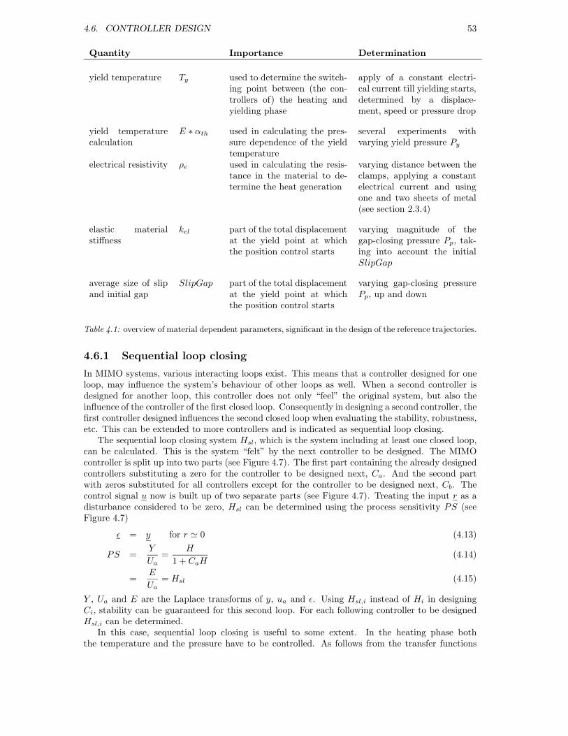
4.6. CONTROLLER DESIGN 53
Quantity Importance Determination
yield temperature Ty used to determine the switch-ing point between (the con-trollers of) the heating andyielding phase
apply of a constant electri-cal current till yielding starts,determined by a displace-ment, speed or pressure drop
yield temperaturecalculation
E ∗ αth used in calculating the pres-sure dependence of the yieldtemperature
several experiments withvarying yield pressure Py
electrical resistivity ρe used in calculating the resis-tance in the material to de-termine the heat generation
varying distance between theclamps, applying a constantelectrical current and usingone and two sheets of metal(see section 2.3.4)
elastic materialstiffness
kel part of the total displacementat the yield point at whichthe position control starts
varying magnitude of thegap-closing pressure Pp, tak-ing into account the initialSlipGap
average size of slipand initial gap
SlipGap part of the total displacementat the yield point at whichthe position control starts
varying gap-closing pressurePp, up and down
Table 4.1: overview of material dependent parameters, significant in the design of the reference trajectories.
4.6.1 Sequential loop closing
In MIMO systems, various interacting loops exist. This means that a controller designed for oneloop, may influence the system’s behaviour of other loops as well. When a second controller isdesigned for another loop, this controller does not only “feel” the original system, but also theinfluence of the controller of the first closed loop. Consequently in designing a second controller, thefirst controller designed influences the second closed loop when evaluating the stability, robustness,etc. This can be extended to more controllers and is indicated as sequential loop closing.
The sequential loop closing system Hsl, which is the system including at least one closed loop,can be calculated. This is the system “felt” by the next controller to be designed. The MIMOcontroller is split up into two parts (see Figure 4.7). The first part containing the already designedcontrollers substituting a zero for the controller to be designed next, Ca. And the second partwith zeros substituted for all controllers except for the controller to be designed next, Cb. Thecontrol signal u now is built up of two separate parts (see Figure 4.7). Treating the input r as adisturbance considered to be zero, Hsl can be determined using the process sensitivity PS (seeFigure 4.7)
ε = y for r ' 0 (4.13)
PS =Y
Ua
=H
1 + CaH(4.14)
=E
Ua
= Hsl (4.15)
Y , Ua and E are the Laplace transforms of y, ua and ε. Using Hsl,i instead of Hi in designingCi, stability can be guaranteed for this second loop. For each following controller to be designedHsl,i can be determined.
In this case, sequential loop closing is useful to some extent. In the heating phase boththe temperature and the pressure have to be controlled. As follows from the transfer functions
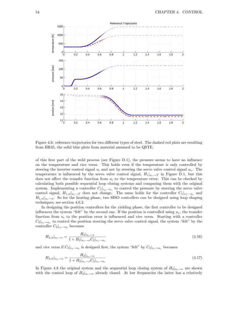
54 CHAPTER 4. CONTROL
0 0.2 0.4 0.6 0.8 1 1.2 1.4 1.6 1.8 211
12
13
14
15
posi
tion
[mm
]0 0.2 0.4 0.6 0.8 1 1.2 1.4 1.6 1.8 2
0
500
1000
1500
tem
pera
ture
[K]
Reference Trajectories
0 0.2 0.4 0.6 0.8 1 1.2 1.4 1.6 1.8 20
50
100
150
pres
sure
[bar
]
Figure 4.6: reference trajectories for two different types of steel. The dashed red plots are resultingfrom HR45, the solid blue plots from material assumed to be QSTE.
of this first part of the weld process (see Figure D.1), the pressure seems to have no influenceon the temperature and vice versa. This holds even if the temperature is only controlled bysteering the inverter control signal ui and not by steering the servo valve control signal uv. Thetemperature is influenced by the servo valve control signal, H1|uv→T in Figure D.1, but thisdoes not affect the transfer function from ui to the temperature error. This can be checked bycalculating both possible sequential loop closing systems and comparing them with the originalsystem. Implementing a controller C1|εp→uv
to control the pressure by steering the servo valvecontrol signal, H1,sl|ui→T does not change. The same holds for the controller C1|εT →ui
andH1,sl|uv→x. So for the heating phase, two SISO controllers can be designed using loop shapingtechniques, see section 4.6.2.
In designing the position controllers for the yielding phase, the first controller to be designedinfluences the system “felt” by the second one. If the position is controlled using uv, the transferfunction from ui to the position error is influenced and vice versa. Starting with a controllerC2|εx→uv
to control the position steering the servo valve control signal, the system “felt” by thecontroller C2|εx→ui
becomes
H2,sl|ui→x =H2|ui→x
1 + H2|uv→xC2|εx→uv
(4.16)
and vice versa if C2|εx→uiis designed first, the system “felt” by C2|εx→uv
becomes
H2,sl|uv→x =H2|uv→x
1 + H2|ui→xC2|εx→ui
(4.17)
In Figure 4.8 the original system and the sequential loop closing system of H2|ui→x are shownwith the control loop of H2|uv→x already closed. At low frequencies the latter has a relatively
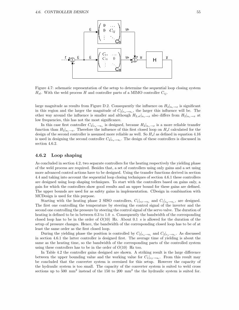
4.6. CONTROLLER DESIGN 55
H
ub
Se
S
e
e ua +
+
u yr +
-
Ca
Cb
Figure 4.7: schematic representation of the setup to determine the sequential loop closing systemHsl. With the weld process H and controller parts of a MIMO controller Cij .
large magnitude as results from Figure D.2. Consequently the influence on H2|ui→x is significantin this region and the larger the magnitude of C2|εx→uv
, the larger this influence will be. Theother way around the influence is smaller and although H2,sl|uv→x also differs from H2|uv→x atlow frequencies, this has not the most significance.
In this case first controller C2|εx→uvis designed, because H2|uv→x is a more reliable transfer
function than H2|ui→x. Therefore the influence of this first closed loop on Hsl calculated for thedesign of the second controller is assumed more reliable as well. So Hsl as defined in equation 4.16is used in designing the second controller C2|εx→ui
. The design of these controllers is discussed insection 4.6.2.
4.6.2 Loop shaping
As concluded in section 4.2, two separate controllers for the heating respectively the yielding phaseof the weld process are required. Besides that, a set of controllers using only gains and a set usingmore advanced control actions have to be designed. Using the transfer functions derived in section4.4 and taking into account the sequential loop closing techniques of section 4.6.1 these controllersare designed using loop shaping techniques. To start with the controllers based on gains only, again for which the controllers show good results and an upper bound for these gains are defined.The upper bounds are used for as safety gains in implementation. CDesign in combination withMCDesign is used for this purpose.
Starting with the heating phase 2 SISO controllers, C1|εT →uiand C1|εp→uv
, are designed.The first one controlling the temperature by steering the control signal of the inverter and thesecond one controlling the pressure by steering the control signal of the servo valve. The duration ofheating is defined to be in between 0.3 to 1.0 s. Consequently the bandwidth of the correspondingclosed loop has to be in the order of O(10) Hz. About 0.1 s is allowed for the duration of thesetup of pressure changes. Hence, the bandwidth of the corresponding closed loop has to be of atleast the same order as the first closed loop.
During the yielding phase the position is controlled by C2|εx→uiand C2|εx→uv
. As discussedin section 4.6.1 the latter controller is designed first. The average time of yielding is about thesame as the heating time, so the bandwidth of the corresponding parts of the controlled systemusing these controllers has to be in the order of O(10) Hz too.
In Table 4.2 the controller gains designed are shown. A striking result is the large differencebetween the upper bounding value and the working value for C1|εT →ui
. From this result maybe concluded that the converter system is oversized for this setup. However the capacity ofthe hydraulic system is too small. The capacity of the converter system is suited to weld crosssections up to 500 mm2 instead of the 150 to 200 mm2 the the hydraulic system is suited for.

56 CHAPTER 4. CONTROL
10−1
100
101
102
103
−200
−150
−100
−50
0
Mag
nitu
de [d
B]
Original system vs sequential loop closing system
10−1
100
101
102
103
−400
−300
−200
−100
0
Pha
se [d
egre
es]
Frequency [Hz]
Figure 4.8: the original system versus the system resulting from sequential loop closing. Thedashed blue plot shows the original transfer function H2|ui→x and the solid red plot the systemactually “felt” by C2|εx→ui
with the control loop of H2|uv→x already closed.
Controller Upper bound Working value
C1|εT →ui0.1 400 Hz 0.004 6 Hz
C1|εp→uv1.2 100 Hz 0.8 65 Hz
C2|εx→uv0.6 2 Hz 0.3 1 Hz
C2|εx→ui15 0.7 Hz 10 0.5 Hz
Table 4.2: feedback controllers, designed using only a gain. The upper bounds as well as working valuesfor the gains are given.

4.6. CONTROLLER DESIGN 57
Controller C2|εx→uiis designed using a gain of 0.05 for C2|εx→uv
. The higher this gain, the higherthe bandwidth of the open loop system H2|ui→xC2|εx→ui
if the gain of C2|εx→uiis increased
simultaneously.Some demands to the closed loop system are not met using the controllers presented in Table
4.2. First, not all demanded bandwidths are reached. Besides that, simulation and experimentalresults show small steady state errors. This can not be solved by controllers using only gains.Consequently controllers using more advanced control techniques have been designed.
The closed loops corresponding to the controllers C1|εT →uiand C1|εp→uv
satisfy the demandedbandwidth (see Table 4.2). Moreover, if necessary, the bandwidths can be increased yet. Howeversimulation and experimental results show small steady state errors. So for both cases applicationof an I-action may be useful. However the present working gain of C1|εT →ui
can be increased thatmuch before it reaches its upper bound, that an I-action is only applied in C1|εp→uv
. This alreadyis discussed in section 3.6.4.
An exact amount of upset resulting after yielding is one of the demands to the controller.However after implementation of the controllers C2|εx→uv
and C2|εT →uv, a small steady state error
in the position response results. Besides that, the demands to the bandwidths of the correspondingclosed loops are only nearly met. First an I-action is applied in C2|εx→uv
. In order to increasethe bandwidth, also damping is added. The open loop system using the original controller aspresented in Table 4.2 and the new controller for two different gains is shown in Figure 4.9. Usinga gain of 7 · 10−5, the corresponding open loop has a bandwidth of 1 Hz and a phase margin of90 deg. Increasing the gain to 6.5 · 10−4 this bandwidth increases to 5.5 Hz. The phase marginhowever decreases to 45 deg (see Figure 4.9). During this study a paper on the modelling andposition control of hydraulic systems has been written [Wijnheijmer & Naus, 2005]. This papercan be used as a guide for this part of the control problem.
−2 −1.5 −1 −0.5 0 0.5 1 1.5 2 2.5−3
−2.5
−2
−1.5
−1
−0.5
0
0.5
1
1.5
Real
Imag
inai
ry
Nyquist plot of C2uv→ x
Figure 4.9: open loop responses of H2|uv→xC2|εx→uv. The dashed blue response shows the open
loop using only a gain for C2|εx→uv. I-action as well as damping is applied in both the other two
responses. The difference between them is a varying gain. The bandwidths of the responses are2 Hz, 1 Hz and 5.5 Hz.
In designing C2|εx→ui, the sequential loop closing system H2,sl|ui→x is used. In the closed loop
present in H2,sl|ui→x, C2|εx→uvof Table 4.3 with a gain of 7 · 10−5 is used. The higher the gain
of C2|εx→uv, the more the gain of C2|εx→ui
can be increased in order to increase the bandwidth
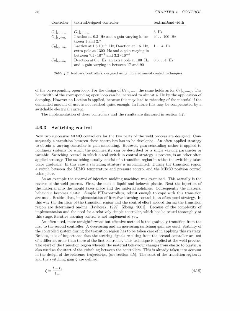
58 CHAPTER 4. CONTROL
Controller textrmDesigned controller textrmBandwidth
C1|εT →uiG1|εT →ui
6 HzC1|εp→uv
I-action at 0.3 Hz and a gain varying in be-tween 1 and 2.7
40 . . . 100 Hz
C2|εx→uvI-action at 1.6·10−4 Hz, D-action at 1.6 Hz,extra pole at 1300 Hz and a gain varying inbetween 7.5 · 10−5 and 3.2 · 10−4
1 . . . 4 Hz
C2|εx→uiD-action at 0.5 Hz, an extra pole at 100 Hzand a gain varying in between 17 and 90
0.5 . . . 4 Hz
Table 4.3: feedback controllers, designed using more advanced control techniques.
of the corresponding open loop. For the design of C2|εx→uithe same holds as for C2|εx→uv
. Thebandwidth of the corresponding open loop can be increased to almost 4 Hz by the application ofdamping. However no I-action is applied, because this may lead to reheating of the material if thedemanded amount of uset is not reached quick enough. In future this may be compensated by aswitchable electrical current.
The implementation of these controllers and the results are discussed in section 4.7.
4.6.3 Switching control
Now two successive MIMO controllers for the two parts of the weld process are designed. Con-sequently a transition between these controllers has to be developed. An often applied strategyto obtain a varying controller is gain scheduling. However, gain scheduling rather is applied tononlinear systems for which the nonlinearity can be described by a single varying parameter orvariable. Switching control in which a real switch in control strategy is present, is an other oftenapplied strategy. The switching usually consist of a transition region in which the switching takesplace gradually. In this case a switching strategy is implemented. During the transition regiona switch between the MIMO temperature and pressure control and the MIMO position controltakes place.
As an example the control of injection molding machines was examined. This actually is thereverse of the weld process. First, the melt is liquid and behaves plastic. Next the injection ofthe material into the mould takes place and the material solidifies. Consequently the materialbehaviour becomes elastic. Simple PID-controllers, robust enough to cope with this transitionare used. Besides that, implementation of iterative learning control is an often used strategy. Inthis way the duration of the transition region and the control effort needed during the transitionregion are determined on-line [Havlicsek, 1999], [Zheng, 2001]. Because of the complexity ofimplementation and the need for a relatively simple controller, which has be tested thoroughly atthis stage, iterative learning control is not implemented yet.
An often used, more straightforward but effective method is the gradually transition from thefirst to the second controller. A decreasing and an increasing switching gain are used. Stability ofthe controlled system during the transition region has to be taken care of in applying this strategy.Besides, it is of importance that the steering signals resulting from the second controller are notof a different order than those of the first controller. This technique is applied at the weld process.The start of the transition region wherein the material behaviour changes from elastic to plastic, isalso used as the start of the switching between the controllers. This is already taken into accountin the design of the reference trajectories, (see section 4.5). The start of the transition region t1and the switching gain ζ are defined:
ζ =t − t1tsw
(4.18)

4.6. CONTROLLER DESIGN 59
with tsw the duration of the transition region. The controller during switching now becomes
C1→2 = ζC2 + (1 − ζ)C1 for t1 ≤ t ≤ t1 + tsw (4.19)
C1 controls the temperature and pressure progress and C2 the position progress. Hence, dif-ferent parts of the MIMO controller C1→2 are used. Consequently, the decrease and increase inswitching gains during the transition region does not lead to stability problems if the controllersare considered separately. However, although different input-output responses are used, the closedloops influence each other nevertheless because of the MIMO nature of the system (see section4.6.1). Stability during the transition region is guaranteed if all open loops, based on the appro-priate sequential loop closing system rather than the original system, are stable. Consequentlythe sequential loop closing systems of the various parts of C1→2 are determined. The concerningopen loops are taken as the last ones to close. In this way stability is guaranteed. This is done forthe controllers defined in Table 4.2 as well as for the controllers presented in Table 4.3.
Using the controllers as defined in Table 4.2, the MIMO switching controller C1→2 is stable ∀tduring switching. In Figure 4.10 the open loop C1→2|εP→uv
H1→2,sl|uv→P is shown for varying t.For C1→2|εP→uv
only the gains of Table 4.2 are used, so the increasing influence of the positioncontrollers with increasing t is obvious. The open loop system remains stable ∀t all the same.
10−4
10−3
10−2
10−1
100
101
102
103
104
−150
−100
−50
0
50
Mag
nitu
de [d
B]
Open loop transfer functions of C1→ 2ε P→ uvH1→ 2,sl
uv→ P
10−4
10−3
10−2
10−1
100
101
102
103
104
−300
−200
−100
0
100
200
Pha
se [d
egre
es]
Frequency [Hz]
Figure 4.10: progress of the open loop system C1→2|εP→uvH1→2,sl|uv→P during the transition
region using the controllers defined in Table 4.2. t = t1 yields the dashed blue plot, t = t1 +0.5tsw
yields the solid red plot and t = t1 + 0.9tsw the (light) green plot.
Next the more advanced controllers as defined in Table 4.3 are tested using average gains. TheMIMO switching controller C1→2 again appears to be stable ∀t during the transition region. InFigure 4.11 the Nyquist responses of C1→2|εx→uv
H1→2,sl|uv→x are shown for varying t (see alsoFigure 4.9). The dash-dotted black plot shows the final controller C2|εx→uv
. The dashed blueto the solid (light) green plot show C1→2|εx→uv
for various t. From this is concluded that theswitching controller C1→2 (see equation 4.19) is stable ∀t during the transition region.
4.6.4 Learning control
In the original assignment learning control was proposed as part of the new strategy because ofthe high level of repetition of the process. Within the framework of this study only time was
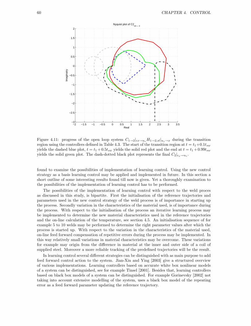
60 CHAPTER 4. CONTROL
−2 −1.5 −1 −0.5 0 0.5 1 1.5 2 2.5 3 3.5−3
−2.5
−2
−1.5
−1
−0.5
0
0.5
1
1.5
2
Real
Imag
inai
ry
Nyquist plot of C2uv→ x
Figure 4.11: progress of the open loop system C1→2|εx→uvH1→2,sl|uv→x during the transition
region using the controllers defined in Table 4.3. The start of the transition region at t = t1+0.1tsw
yields the dashed blue plot, t = t1 +0.5tsw yields the solid red plot and the end at t = t1 +0.99tsw
yields the solid green plot. The dash-dotted black plot represents the final C2|εx→uv.
found to examine the possibilities of implementation of learning control. Using the new controlstrategy as a basis learning control may be applied and implemented in future. In this section ashort outline of some interesting results found till now is given. Yet a thoroughly examination tothe possibilities of the implementation of learning control has to be performed.
The possibilities of the implementation of learning control with respect to the weld procesas discussed in this study, is bipartite. First the initialisation of the reference trajectories andparameters used in the new control strategy of the weld process is of importance in starting upthe process. Secondly variation in the characteristics of the material used, is of importance duringthe process. With respect to the initialisation of the process an iterative learning process maybe implemented to determine the new material characteristics used in the reference trajectoriesand the on-line calculation of the temperature, see section 4.5. An initialisation sequence of forexample 5 to 10 welds may be performed to determine the right parameter values after which theprocess is started up. With respect to the variation in the characteristics of the material used,on-line feed forward compensation of repetitive errors during the process may be implemented. Inthis way relatively small variations in material characteristics may be overcome. These variationsfor example may origin from the difference in material at the inner and outer side of a coil ofsupplied steel. Moreover a more reliable tracking of the predefined trajectories will be the result.
In learning control several different strategies can be distinguished with as main purpose to addfeed forward control action to the system. Jian-Xin and Ying [2003] give a structured overviewof various implementations. Learning controllers based on accurate white box nonlinear modelsof a system can be distinguished, see for example Tinsel [2001]. Besides that, learning controllersbased on black box models of a system can be distinguished. For example Gorinevsky [2002] nottaking into account extensive modelling of the system, uses a black box model of the repeatingerror as a feed forward parameter updating the reference trajectory.
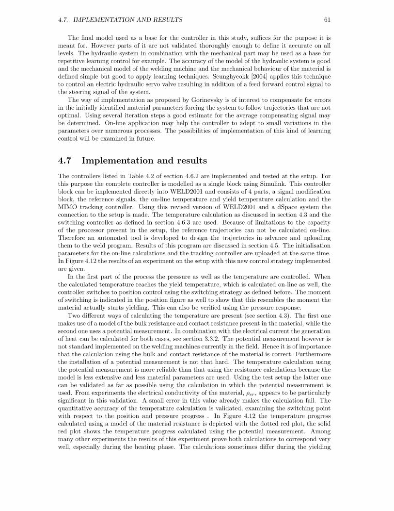
4.7. IMPLEMENTATION AND RESULTS 61
The final model used as a base for the controller in this study, suffices for the purpose it ismeant for. However parts of it are not validated thoroughly enough to define it accurate on alllevels. The hydraulic system in combination with the mechanical part may be used as a base forrepetitive learning control for example. The accuracy of the model of the hydraulic system is goodand the mechanical model of the welding machine and the mechanical behaviour of the material isdefined simple but good to apply learning techniques. Seunghyeokk [2004] applies this techniqueto control an electric hydraulic servo valve resulting in addition of a feed forward control signal tothe steering signal of the system.
The way of implementation as proposed by Gorinevsky is of interest to compensate for errorsin the initially identified material parameters forcing the system to follow trajectories that are notoptimal. Using several iteration steps a good estimate for the average compensating signal maybe determined. On-line application may help the controller to adept to small variations in theparameters over numerous processes. The possibilities of implementation of this kind of learningcontrol will be examined in future.
4.7 Implementation and results
The controllers listed in Table 4.2 of section 4.6.2 are implemented and tested at the setup. Forthis purpose the complete controller is modelled as a single block using Simulink. This controllerblock can be implemented directly into WELD2001 and consists of 4 parts, a signal modificationblock, the reference signals, the on-line temperature and yield temperature calculation and theMIMO tracking controller. Using this revised version of WELD2001 and a dSpace system theconnection to the setup is made. The temperature calculation as discussed in section 4.3 and theswitching controller as defined in section 4.6.3 are used. Because of limitations to the capacityof the processor present in the setup, the reference trajectories can not be calculated on-line.Therefore an automated tool is developed to design the trajectories in advance and uploadingthem to the weld program. Results of this program are discussed in section 4.5. The initialisationparameters for the on-line calculations and the tracking controller are uploaded at the same time.In Figure 4.12 the results of an experiment on the setup with this new control strategy implementedare given.
In the first part of the process the pressure as well as the temperature are controlled. Whenthe calculated temperature reaches the yield temperature, which is calculated on-line as well, thecontroller switches to position control using the switching strategy as defined before. The momentof switching is indicated in the position figure as well to show that this resembles the moment thematerial actually starts yielding. This can also be verified using the pressure response.
Two different ways of calculating the temperature are present (see section 4.3). The first onemakes use of a model of the bulk resistance and contact resistance present in the material, while thesecond one uses a potential measurement. In combination with the electrical current the generationof heat can be calculated for both cases, see section 3.3.2. The potential measurement however isnot standard implemented on the welding machines currently in the field. Hence it is of importancethat the calculation using the bulk and contact resistance of the material is correct. Furthermorethe installation of a potential measurement is not that hard. The temperature calculation usingthe potential measurement is more reliable than that using the resistance calculations because themodel is less extensive and less material parameters are used. Using the test setup the latter onecan be validated as far as possible using the calculation in which the potential measurement isused. From experiments the electrical conductivity of the material, ρer, appears to be particularlysignificant in this validation. A small error in this value already makes the calculation fail. Thequantitative accuracy of the temperature calculation is validated, examining the switching pointwith respect to the position and pressure progress . In Figure 4.12 the temperature progresscalculated using a model of the material resistance is depicted with the dotted red plot, the solidred plot shows the temperature progress calculated using the potential measurement. Amongmany other experiments the results of this experiment prove both calculations to correspond verywell, especially during the heating phase. The calculations sometimes differ during the yielding
62 CHAPTER 4. CONTROL
0 0.5 1 1.5 211
12
13
14
15
16
Pos
ition
[mm
]
0 0.5 1 1.5 20
500
1000
1500
Tem
pera
ture
[K]
0 0.5 1 1.5 2−20
0
20
40
60
80
100
120
Time [s]
Pre
ssur
e [b
ar]
0 0.5 1 1.5 2−0.1
0
0.1
0.2
0.3
0.4
Time [s]
Inve
rter
con
trol
sig
nal
Figure 4.12: resulting position, temperature, pressure and inverter control signal progress duringthe weld process after implementation of the new control strategy. The dashed blue plots indicatethe reference trajectories and in case of the inverter control signal the command signal to theinverter. The solid red plots show the actual progress of the various parameters and the (light)green plots in the upper right and left Figures show the on-line calculated force dependent yieldtemperature respectively the switch moment when crossing the calculated temperature. Thedotted red plot in the temperature figure results from the second temperature calculation.
phase and further on as is also the matter in this case. However, they resemble very well duringheating, which is the part of the process that is temperature controlled, so for the moment theseresults suffice.
Relatively small gains are used in this example, as can be seen in Figure 4.12. Larger gainsas listed in Table 4.2 are successfully tested as well. A lot of experiments are performed, butthe more advanced controllers listed in Table 4.3 are not implemented and tested yet. Thesecontrollers are tested off-line using a simulation model, ProcessSimulation.mdl in which thedeveloped controller block can be implemented (see Appendix F). The reference trajectories arestill being improved, see for example the trajectories of section 4.5, which are already of a nextgeneration than those used in this example, and as from experiments result, improvement is stillneeded. Especially the transition region from elastic to plastic material behaviour has to be levelledmore to assure a smooth position progress. The transition from elastic to plastic deformation inthe position reference trajectory is not smooth enough yet. Consequently for example dips in theprogress of the electrical current and the pressure are present in the switching region.
The results of the experiment depicted in Figure 4.12 among many other experiments showthat the developed controller performs well. The reference trajectories however, are still beingimproved and the more advanced controllers have to be implemented and tested on-line. Becauseof the highly repetitive character of the process, learning control as outlined in section 4.6.4 is

4.7. IMPLEMENTATION AND RESULTS 63
of great interest to be implemented as well. The on-line temperature calculation used has shownto suffice so far. However the model used has to be validated thoroughly using more reliabletemperature measurements. Furthermore the control strategy is being adapted to suit control ofthe FRW-series welding machines.

64 CHAPTER 4. CONTROL
Chapter 5
Conclusions and recommendations
In this chapter the conclusions and recommendations concerning the assignment are given.
Conclusions
To overcome limitations of the current control of the DC upset resistance weld process, a newcontrol strategy is developed. Consequently a good insight in the process was needed. Thetheoretical insight in the process is renewed and has expanded. The validity of this theory isfounded by experimental results. In this way the theory and assumptions made with respect tothe systems and equilibria present in the process, are shown to be correct. A complete overviewof the systems present in the weld process is given.
As a base for the new control strategy and to validate the expanded insight in the system, amodel of the weld process has been developed. This has resulted in a simulation model, whichcan be used for off-line simulation of the weld process. The model and the theory have beenvalidated by experimental results. The corresponding progress of position, of electrical currentand of pressure exhibit good agreement. The model also gives a good indication of the progress ofthe temperature during the weld process. Special attention is given to the modelling and controlof the hydraulic system. This has resulted in a relatively easy model-based controller developmentthat suits the possibilities of the hydraulic system better than the previous controller. A paperon the modelling and control of hydraulic systems focussing on position control has been writtenduring this study [Wijnheijmer & Naus, 2005].
The simulation model is simplified to suit on-line calculation of the temperature and yieldtemperature. Validation of the on-line calculation shows that the resulting model satisfies thispurpose. In two different ways a good on-line calculation of the temperature progress can bemade now. Linearised frequency responses are determined using the simplified model as a base.These responses are used in further controller development to enable application of loop shapingtechniques. From the linearisation follows that a good approximation of the model can be madeusing two separate linear models. Each model has two inputs and three outputs. Application ofthese linear models shows that only the transfer functions involving the temperature-dependentmaterial behaviour (H2|ui→x and H2|ui→p) are less reliable. The remaining transfer functions aregood representations of the process.
For the first and second part of the weld process, a MIMO controller for both temperature andpressure tracking, respectively for position tracking are designed. A switching strategy controls thetransition between the two controllers assuring stability during switching. Furthermore sequentialloop closing is used to assure stability of each of the MIMO controllers. The reference trajectoriesare based on the results of the developed theory and modelling as well as on practical experience.Consequently, they prescribe a representative progress of the involved variables. Loop shapingtechniques are used to design two sets of controllers satisfying the demanded bandwidths. Thefirst set of controllers is implemented and tested successfully. The second set is implemented only
65
66 CHAPTER 5. CONCLUSIONS AND RECOMMENDATIONS
partly yet, but experimental and simulation show good correspondence. To facilitate working withthe MIMO control problem, MCDesign, a tool for MIMO controller design, has been developed[Wijnheijmer & Naus, 2005].
The resulting controller satisfies the stated requirements: the weld process now is completedwithin a predefined time interval in which a predefined amount of upset is achieved exactly. More-over, the temperature progress during the first part of the process is controlled as well. In thefuture these results can be combined with the NIMR research, which should give rise to an indica-tion of the quality of the weld in advance. The controller is sensitive for some material propertiesdue to the dependence of the on-line calculation of the temperature and yield temperature onthese properties. Because of the highly repetitive character of the process, application of learningcontrol may be useful in solving this problem. A first start to future implementation of learningtechniques in the controller or reference trajectories has been made.
Recommendations
Recommendations are distinguished concerning the results of the assignment and the setup. Therecommendations concerning the results of the assignment:
• More extensive modelling of the mechanics of the material may be performed, especiallyduring the transition from elastic to plastic material behaviour. This may result in animproved design of the corresponding controllers.
• The models used for on-line temperature calculation have to be validated better usingseveral reliable temperature measurements.
• The force needed during the weld process is still determined by trial and error. Theinfluence of the size and the material of the coiled sheets on this force has to be examined.
• Implementation and testing of the more advanced controllers and optimisation of thesecontrollers by extensive testing has to be done.
• Based on literature, the possibilities for the implementation of iterative learning or up-dating techniques are promising. Examination and implementation of learning techniquesmay increase the reliability and robustness of the controller for changing material properties.
• Combining future results of the NIMR giving guidelines for the progress of the weld processwith respect to the quality of a weld and the reference trajectories respectively the developedcontrollers.
The recommendations concerning the setup:
• When the material is clamped, the distance between the clamps instead of the pressure onthe material is controlled This results in a considerable increase in pressure. Hence it maybe replaced by a pressure controller including a position feedback with low gain to preventdrifting.
• Loading the setup and surface conditions of the sheet ends to be welded together havemuch influence on the resulting weld. So loading the welding machine has to becomeunambiguous. If the problems resulting from varying surface conditions remain, a study toinsert an extra operation before the weld process to derive constant surface conditions ofthe sheet ends may be useful.

67
• The influence of a varying initial distance between the clamps has to be examined.
• Further development of the setup as used in this study may be useful to reduce upset andwelding times in future.

68 CHAPTER 5. CONCLUSIONS AND RECOMMENDATIONS

Chapter 6
References
Books and notes1 Bejan, A., Heat transfer, John Wiley & Sons, Inc, 1993.
2 Franklin, G.F., Powell, J.D. and Emami, A., Feedback control of dynamic systems,Addison-Wesley Publishing Company, Inc., third edition, 1994.
3 Jian-Xin Xu, Ying Tan, Linear and Nonlinear Iterative Learning Control, Springer,March 2003.
4 Kokernak, R.P., Fluid power technology, New York, US Imports & PHIPEs, secondedition, 1998
5 Leijendeckers, P.H.H., Fortuin, J.B., Van Herwijnen, F. and Schwippert, G.A., Polytechnisch zakboek, 49th edition, 2002, Elsevier Bedrijfsinformatie B.V., ISBN 90-6228-358-6 geb.
6 Merrit, H., Hydraulic Control Systems, New York US: John Wiley & Sons Inc, firstedition, 1967.
7 Post, W.J.A.E.M. and Teerhuis, P.C., Hydraulic servo control, lecture notes, Universityof Technology Eindhoven, Mechanical Engineering, Control Systems Technology, 2004.
8 Skogestad, S. and Postlethwaite, I., Multivariable feedback control - analysis and design,1996
9 Steinbuch, M. Digital Motion Control, lecture notes, University of Technology Eind-hoven, Mechanical Engineering, Control Systems Technology, 2004.
10 Tochtermann, Bodenstein, Konstruktionselemente des Maschinenbaues, 8th edition, firstpart, 1968.
11 Viersma, T.J., Analysis, Synthesis and Design of Hydraulic Servosystems and Pipelines,Delft University of Technology, revised edition, 1990.
12 Zwolsman, J.O. and Vroomans, H.M., Der Kontakwiderstand beim Widerstandsschweis-sen, DVS Berichte no 124, 1987, p. 122-127.
13 Zwolsman, J.O., Quality in resistance welding: an analysis of the process and its control,Cambridge: Abinton, 1991, ISBN 1-85576-033-2.
69

70 CHAPTER 6. REFERENCES
Reports and papers14 Allersma, et al, Plan van aanpak, graduation report on the start of building the setup,
WA0023, September 2003.
15 Elassal, M.E.H., Modelvorming en krachtregeling van de FHL400 lasmachine, internshipreport on the modelling and control of the weld process as per formed on the FHL series,March 1996.
16 Feng, Z., Gould, J.E., et al, An incrementally coupled electrical-thermal-mechanicalmodel for resistance spot welding, 5th International Conference on Trends in WeldingResearch, Pine Mountain, GA, 1-5 June 1998.
17 Fontijne Grotnes B.V., Improved technology to DC butt welding, DC-press butt weldingfor car and truck rims, called FRW-series since 2001
18 Gorinevsky, Dimitry, Loop Shaping for Iterative Control of Batch Processes, IEEE Con-trol Systems Magazine, December 2002.
19 Havlicsek, H. and A. Alleyne, Nonlinear Control of an Electrohydraulic Injection MoldingMachine via Iterative Adaptive Learning, IEEE/ASME Transactions on Mechatronics,Vol. 4, No. 3, pp. 312-323, September 1999.
20 Kucklick, F.C., Flashless DC welding of rims offers advantages, Welding Journal, July,1996.
21 Ledeuil, M., FHL300 - Een nieuw concept, internship report on the concept of the setup,WA0024, November 1998.
22 Legemaate, R., Dynamisch gedrag van een lasproces, internship report on the weld pro-cess as performed on the FHL series, May 1997.
23 Legemaate, R., Beheersing van het lasproces op de Fontijne Holland Lasmachine, grad-uation report on modelling and control of the DC upset resistance weld process, March1998.
24 Louter, R., De bepaling van meetspecificaties en selectie van sensoren voor een experi-mentele lasmachine, internship report on the specifications and measurement equipmentof the setup, WA0022, December 1999.
25 Mast, S.E.P., Analyse van het weerstandstuiklasproces, internship report on the qualityof a weld, May 2000.
26 Meulenberg, R., De beschrijving van het weerstandstuiklasproces van wielvelgen, gradu-ation report, August 2002.
27 Put, R.P., De invloed van de stuikweg bij het weerstanddruklassen van R-St37-2, gradua-tion report on the modelling of the weld process as performed on the FHL series, August1999.
28 Seunghyeokk James Lee, Tsu-Chin Tsao, Repetitive learning of backstepping controllednonlinear electrohydraulic material testing system, Control Engineering Practive 12,1393-1408, 2004.
29 Tinsel, R.B.G., Iterative Learning Control for a Gantry type manipulator, graduationreport, April 2001
30 Wijnheijmer, F.P. and Naus, G.J.L., On the modelling and control of hydraulic systems,paper, 2005.
31 Zheng, D. and A. Alleyne, Modeling and Control of an Electrohydraulic Injection Mold-ing Machine with Smoothed Fill-to-Pack Transition, ASME Journal of ManufacturingScience and Engineering, October, 2001.
71
Applications32 Convert, Convert, http://www.joshmadison.com/software, version 4.08, 1998.
33 DIET, Do It Easy Tool, DIET, http://www.dct.tue.nl/home of diet.htm, University ofTechnology Eindhoven, Mechanical Engineering, Control Systems Technology Group,2003.
34 MCDesign, MCDesign, MIMO controller design tool including MDesign, CDesign andFDesign, Wijnheijmer, F.P., and Naus, G.J.L., version 2.0β, 2005.
35 WELD2000, WELD2000, the DC Weld control retrofit package, Fontijne Grotnes B.V.,software package, 2000.
Internet pages36 aluSELECT, http://aluminium.matter.org.uk/aluselect, computer-based reference
database containing technical information on the most widely used aluminium alloys,partnership between the European Aluminium Association and the MATTER project,2001.
37 Automation International Inc., http://www.automation-intl.com/, automated weldingand metalworking machines.
38 Bosch Rexroth AG, www.boschrexroth.com/.../products/brc/ProductDirectory/CurrentProducts/Welding/PSQ/087004-101-de+en-ws.pdf, Electric Drives and ControlsDivision.
39 Fontijne Grotnes B.V., http://www.fontijnegrotnes.com, homepage of the FontijneGrotnes B.V. company.
40 Hess Industries inc., http://www.hess-eng.com/pages/wrttech.html, Sabre weld control,Wheel and Rim Technologies, Hess Engineering.
41 Infrared Servics Inc., http://www.infrared-thermography.com/material.htm, emissivityvalues for common materials.
42 Key to steel, http://www.key-to-steel.com/articles/art75.htm, steel database - weld pro-cesses, INI International, 2003.
43 Matweb, http://www.matweb.com, material property data for metals, plastics ceramicsand composites.
44 Medar, http://www.medar.com/controls/index.html, Welding Technology Corporation.
45 MOOG Inc., http://www.moog.com, manufacturer of precision control components andsystems, 2005.
46 NIMR, http://www.nimr.nl, Netherlands Institute for Metal Research, 2005.
47 Nonferrous Products, Inc., http://www.nonferrousproducts.com/material%20selection.htm,nonferrous materials database, 2004.
48 NSRW, http://www.nsrw.com/components/weldcomputer.htm 2004, new southern resis-tance welding, Pelham, Alabama.
49 Wolfram research, http://scienceworld.wolfram.com/physics, Eric Weisstein’s world ofscience.

72 CHAPTER 6. REFERENCES
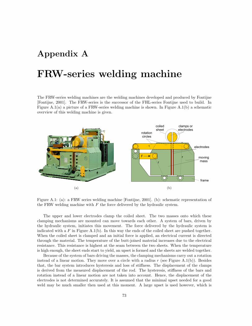
Appendix A
FRW-series welding machine
The FRW-series welding machines are the welding machines developed and produced by Fontijne[Fontijne, 2001]. The FRW-series is the successor of the FHL-series Fontijne used to build. InFigure A.1(a) a picture of a FRW-series welding machine is shown. In Figure A.1(b) a schematicoverview of this welding machine is given.
(a)
movingmass
coiledsheet
frame
clamps orelectrodes
F
r
rotationcircles
electrodes
r
(b)
Figure A.1: (a): a FRW series welding machine [Fontijne, 2001]. (b): schematic representation ofthe FRW welding machine with F the force delivered by the hydraulic system.
The upper and lower electrodes clamp the coiled sheet. The two masses onto which theseclamping mechanisms are mounted can move towards each other. A system of bars, driven bythe hydraulic system, initiates this movement. The force delivered by the hydraulic system isindicated with a F in Figure A.1(b). In this way the ends of the coiled sheet are pushed together.When the coiled sheet is clamped and an initial force is applied, an electrical current is directedthrough the material. The temperature of the butt-joined material increases due to the electricalresistance. This resistance is highest at the seam between the two sheets. When the temperatureis high enough, the sheet ends start to yield, an upset is formed and the sheets are welded together.
Because of the system of bars driving the masses, the clamping mechanisms carry out a rotationinstead of a linear motion. They move over a circle with a radius r (see Figure A.1(b)). Besidesthat, the bar system introduces hysteresis and loss of stiffness. The displacement of the clampsis derived from the measured displacement of the rod. The hysteresis, stiffness of the bars androtation instead of a linear motion are not taken into account. Hence, the displacement of theelectrodes is not determined accurately. It is assumed that the minimal upset needed for a goodweld may be much smaller then used at this moment. A large upset is used however, which is
73

74 APPENDIX A. FRW-SERIES WELDING MACHINE
partly due to the inaccuracy of the position measurement.
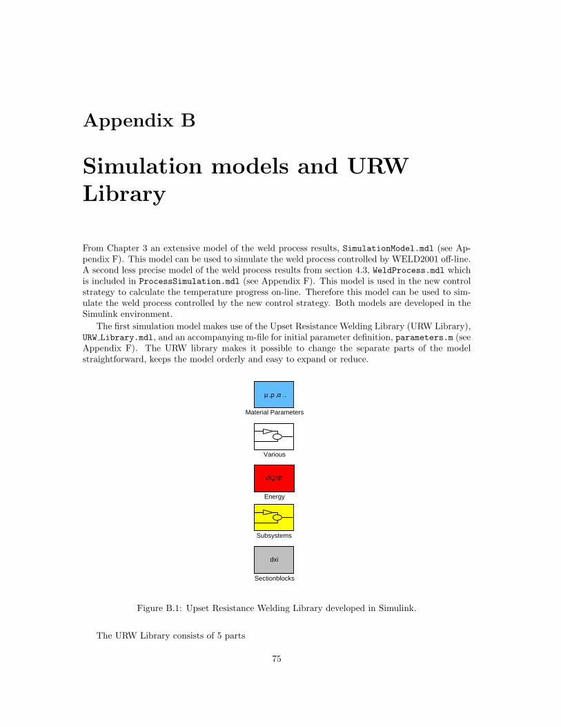
Appendix B
Simulation models and URWLibrary
From Chapter 3 an extensive model of the weld process results, SimulationModel.mdl (see Ap-pendix F). This model can be used to simulate the weld process controlled by WELD2001 off-line.A second less precise model of the weld process results from section 4.3, WeldProcess.mdl whichis included in ProcessSimulation.mdl (see Appendix F). This model is used in the new controlstrategy to calculate the temperature progress on-line. Therefore this model can be used to sim-ulate the weld process controlled by the new control strategy. Both models are developed in theSimulink environment.
The first simulation model makes use of the Upset Resistance Welding Library (URW Library),URW Library.mdl, and an accompanying m-file for initial parameter definition, parameters.m (seeAppendix F). The URW library makes it possible to change the separate parts of the modelstraightforward, keeps the model orderly and easy to expand or reduce.
Various
Subsystems
dxi
Sectionblocks
µ ,ρ ,α ..
Material Parameters
dQ/dt
Energy
Figure B.1: Upset Resistance Welding Library developed in Simulink.
The URW Library consists of 5 parts
75
76 APPENDIX B. SIMULATION MODELS AND URW LIBRARY
• Material Parameters light blue blocks containing models for the temperature depen-dent parameters.
• Energy red blocks including the energy terms are used in the balances of energy of everysection. Each term described in section 3.3 is built-in in this library.
• Subsystems yellow blocks containing various frequently used larger groups of blocks.
• Section blocks grey blocks representing the sections in the working area. The sectionsas resulting from the discretisation of the various parts in the working area (see section3.3.1) and including the accompanying balances of energy and mechanics.
• Various various small user-defined functions.
The weld program WELD2001 is categorised in the section blocks of the URW Library. Geo-metrical, process and temperature independent material parameters are defined in the accompa-nying m-file parameters.m and included in the model by cyan colored blocks.
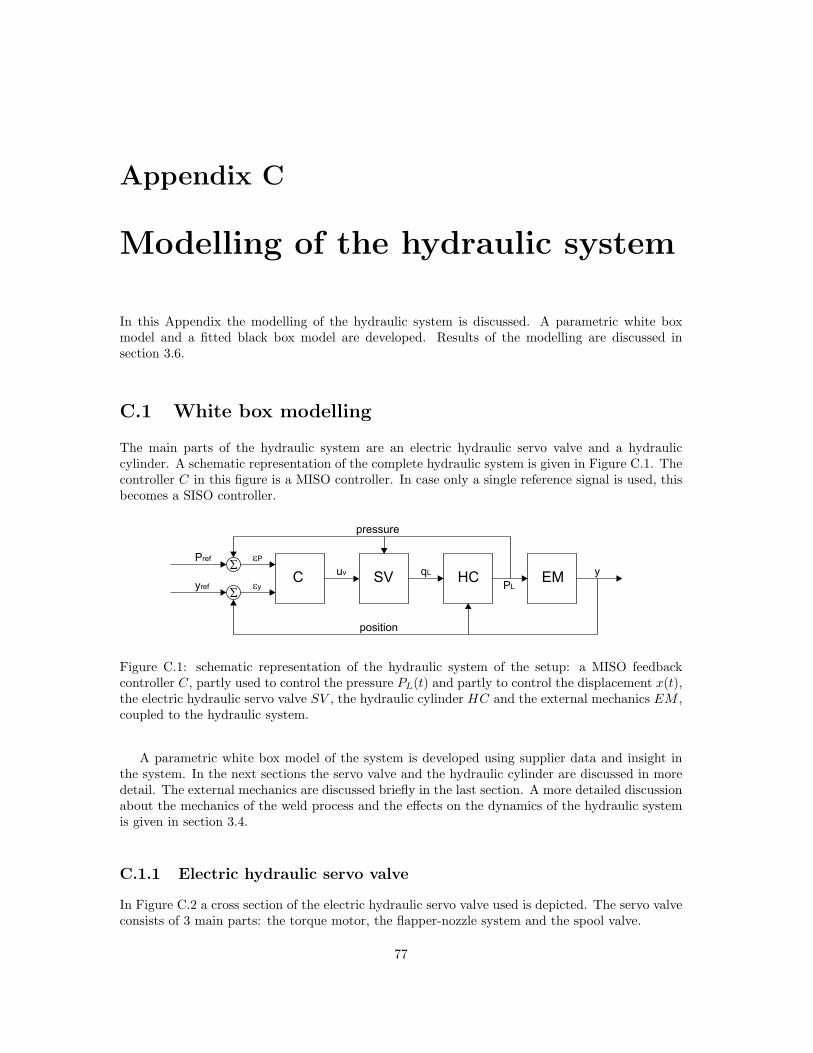
Appendix C
Modelling of the hydraulic system
In this Appendix the modelling of the hydraulic system is discussed. A parametric white boxmodel and a fitted black box model are developed. Results of the modelling are discussed insection 3.6.
C.1 White box modelling
The main parts of the hydraulic system are an electric hydraulic servo valve and a hydrauliccylinder. A schematic representation of the complete hydraulic system is given in Figure C.1. Thecontroller C in this figure is a MISO controller. In case only a single reference signal is used, thisbecomes a SISO controller.
C HCuv qL
S
position
yref
ePPrefS
eyEMSV
PL
pressure
y
Figure C.1: schematic representation of the hydraulic system of the setup: a MISO feedbackcontroller C, partly used to control the pressure PL(t) and partly to control the displacement x(t),the electric hydraulic servo valve SV , the hydraulic cylinder HC and the external mechanics EM ,coupled to the hydraulic system.
A parametric white box model of the system is developed using supplier data and insight inthe system. In the next sections the servo valve and the hydraulic cylinder are discussed in moredetail. The external mechanics are discussed briefly in the last section. A more detailed discussionabout the mechanics of the weld process and the effects on the dynamics of the hydraulic systemis given in section 3.4.
C.1.1 Electric hydraulic servo valve
In Figure C.2 a cross section of the electric hydraulic servo valve used is depicted. The servo valveconsists of 3 main parts: the torque motor, the flapper-nozzle system and the spool valve.
77
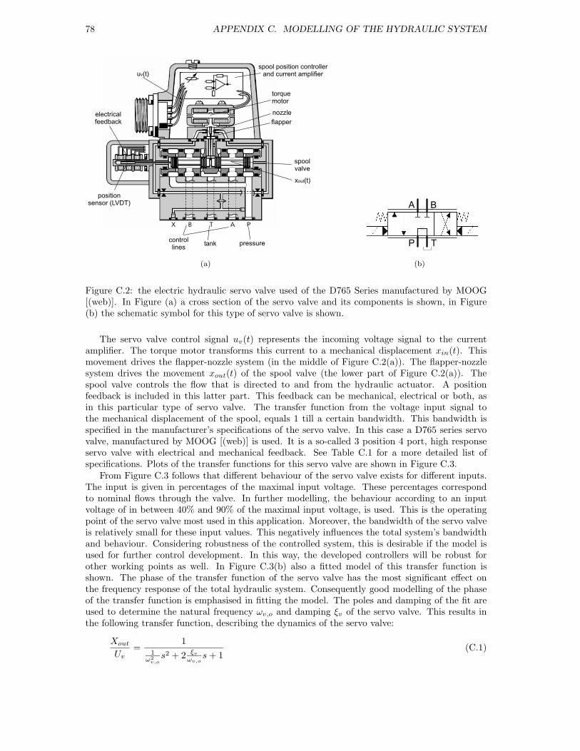
78 APPENDIX C. MODELLING OF THE HYDRAULIC SYSTEM
torquemotor
electricalfeedback
spoolvalve
pressuretank
u (t)v
nozzle
flapper
controllines
x (t)out
positionsensor (LVDT)
spool position controllerand current amplifier
(a)
A B
P T
(b)
Figure C.2: the electric hydraulic servo valve used of the D765 Series manufactured by MOOG[(web)]. In Figure (a) a cross section of the servo valve and its components is shown, in Figure(b) the schematic symbol for this type of servo valve is shown.
The servo valve control signal uv(t) represents the incoming voltage signal to the currentamplifier. The torque motor transforms this current to a mechanical displacement xin(t). Thismovement drives the flapper-nozzle system (in the middle of Figure C.2(a)). The flapper-nozzlesystem drives the movement xout(t) of the spool valve (the lower part of Figure C.2(a)). Thespool valve controls the flow that is directed to and from the hydraulic actuator. A positionfeedback is included in this latter part. This feedback can be mechanical, electrical or both, asin this particular type of servo valve. The transfer function from the voltage input signal tothe mechanical displacement of the spool, equals 1 till a certain bandwidth. This bandwidth isspecified in the manufacturer’s specifications of the servo valve. In this case a D765 series servovalve, manufactured by MOOG [(web)] is used. It is a so-called 3 position 4 port, high responseservo valve with electrical and mechanical feedback. See Table C.1 for a more detailed list ofspecifications. Plots of the transfer functions for this servo valve are shown in Figure C.3.
From Figure C.3 follows that different behaviour of the servo valve exists for different inputs.The input is given in percentages of the maximal input voltage. These percentages correspondto nominal flows through the valve. In further modelling, the behaviour according to an inputvoltage of in between 40% and 90% of the maximal input voltage, is used. This is the operatingpoint of the servo valve most used in this application. Moreover, the bandwidth of the servo valveis relatively small for these input values. This negatively influences the total system’s bandwidthand behaviour. Considering robustness of the controlled system, this is desirable if the model isused for further control development. In this way, the developed controllers will be robust forother working points as well. In Figure C.3(b) also a fitted model of this transfer function isshown. The phase of the transfer function of the servo valve has the most significant effect onthe frequency response of the total hydraulic system. Consequently good modelling of the phaseof the transfer function is emphasised in fitting the model. The poles and damping of the fit areused to determine the natural frequency ωv,o and damping ξv of the servo valve. This results inthe following transfer function, describing the dynamics of the servo valve:
Xout
Uv
=1
1ω2
v,os2 + 2 ξv
ωv,os + 1
(C.1)
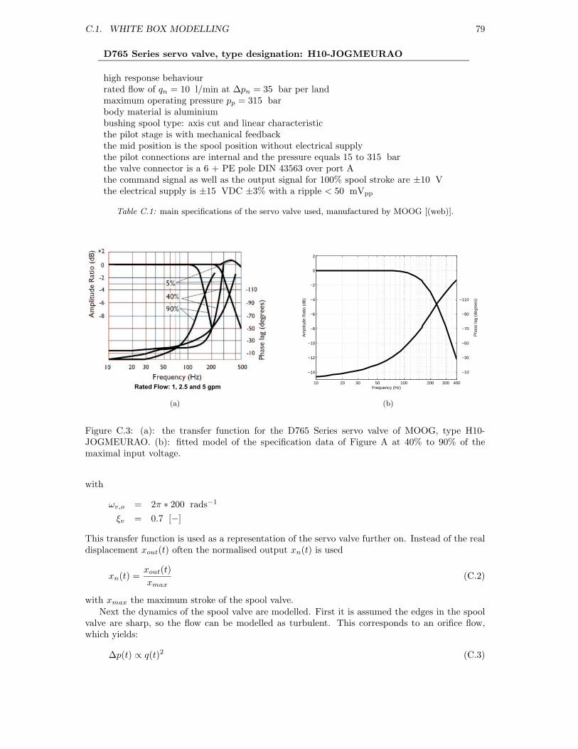
C.1. WHITE BOX MODELLING 79
D765 Series servo valve, type designation: H10-JOGMEURAO
high response behaviourrated flow of qn = 10 l/min at ∆pn = 35 bar per landmaximum operating pressure pp = 315 barbody material is aluminiumbushing spool type: axis cut and linear characteristicthe pilot stage is with mechanical feedbackthe mid position is the spool position without electrical supplythe pilot connections are internal and the pressure equals 15 to 315 barthe valve connector is a 6 + PE pole DIN 43563 over port Athe command signal as well as the output signal for 100% spool stroke are ±10 Vthe electrical supply is ±15 VDC ±3% with a ripple < 50 mVpp
Table C.1: main specifications of the servo valve used, manufactured by MOOG [(web)].
Rated Flow: 1, 2.5 and 5 gpm
(a)
10 20 30 50 100 200 300 400
−14
−12
−10
−8
−6
−4
−2
0
2
Frequency (Hz)
Am
plitu
de R
atio
(dB
)
Pha
se la
g (d
egre
es)
−10
−30
−50
−70
−90
−110
(b)
Figure C.3: (a): the transfer function for the D765 Series servo valve of MOOG, type H10-JOGMEURAO. (b): fitted model of the specification data of Figure A at 40% to 90% of themaximal input voltage.
with
ωv,o = 2π ∗ 200 rads−1
ξv = 0.7 [−]
This transfer function is used as a representation of the servo valve further on. Instead of the realdisplacement xout(t) often the normalised output xn(t) is used
xn(t) =xout(t)
xmax
(C.2)
with xmax the maximum stroke of the spool valve.Next the dynamics of the spool valve are modelled. First it is assumed the edges in the spool
valve are sharp, so the flow can be modelled as turbulent. This corresponds to an orifice flow,which yields:
∆p(t) ∝ q(t)2 (C.3)

80 APPENDIX C. MODELLING OF THE HYDRAULIC SYSTEM
The volume flow q(t) through the control piston then equals [Viersma, 1990], [Merrit, 1967]:
q(t) = bx(t)cd
√
∆p(t) (C.4)
with b the diameter, cd a compensation factor and x(t) the length of the gap. This length iscontrolled by the flapper-nozzle system. From Figure C.4 it follows that
p1(t) =1
2ps +
1
2pl(t) = ppump = ps (C.5)
p2(t) =1
2ps −
1
2pl(t) = ptank = 0 (C.6)
with ps the supply pressure. The servo valve used is a critical center valve, so the overlap ε = 0.Solving equation C.4 for x ≤ 0 and x ≥ 0 and using equations C.5 and C.6, yields
ql(t) =
qnxn(t)√
1 + pn(t) for x > 00 for x = 0
qnxn(t)√
1 − pn(t) for x < 0
(C.7)
(C.8)
with xn(t) the normalised position of the spool valve as defined in equation C.2, and qn(t) thenormalised flow through the servo valve at the normalised pressure pn(t).
qn = bxmaxcd
√
ps
2(C.9)
= q|x=xmaxω∆p (C.10)
pn(t) =pl
ps
(C.11)
Assuming the sign of pn and xn to correspond, the result is a nonlinear equation describing theflow to the hydraulic cylinder
ql(t)
qn
= xn(t)√
1 − pn(t)sign(xn(t)) (C.12)
Equation C.12 is linearised for small variations (xe, pe) around (xo, po) = (η, 0). The equation cannot be linearised around x = 0, since it only holds for turbulent flows. For very small values of xthe flow becomes laminar. The following linearised equation results
ql(t)
qn
= xn −pn(t)
2sign(xn(t)) (C.13)
Besides that, linearisation of the sign-function is not possible. It is thus approached by an atan-function:
ql(t)
qn
= xn(t) −pn(t)
πatan(Gxn(t)) (C.14)
The higher gain G, the better equation C.14 resembles equation C.13.
C.1.2 Hydraulic cylinder
The hydraulic cylinder used in the setup is a double acting, double end-rod cylinder.

C.1. WHITE BOX MODELLING 81
y(t)
Aeff
q *(t)inq (t)outq *(t)out q (t)in
1 2d
dpdpr
qL
piston rod
F(t)
Figure C.4: schematic representation of the hydraulic servo system.
In Figure C.4 a schematic representation of the hydraulic cylinder in combination with theservo valve is shown. The leak flow over the rod bearings is neglected. Some properties of thehydraulic cylinder are listed in Table C.2. The rod is attached to the setup, driving the horizontalmovement of the clamping mechanism (see Figure 2.1(a)). The displacement of the rod is measuredusing a linear variable differential transducer (LVDT), which is attached to one end of the rod.The pressure difference between the two cylinder chambers is measured by a differential pressuregauge. The resulting displacement y(t) and pressure pL(t) is controlled by the flow, which iscontrolled by the servo valve.
description quantity magnitude unitymaximum stroke L 30 · 10−3 moil stiffness [Meulenberg, 2002] Eoil 8 · 108 Nm−1
piston diameter dp 65 · 10−3 mrod diameter dpr 40 · 10−3 m
Table C.2: properties of the hydraulic cylinder.
A dynamic model of the hydraulic cylinder is derived using the balance of mass. For a singlecylinder chamber this balance equals
dMi(t)
dt=
∑
Φi(t) (C.15)
= Φin,i(t) − Φout,i(t)
with Φi(t) the mass flow rate of cylinder chamber i:
Φi(t) = ρi(t)qi(t) (C.16)
with qi(t) the volume flow rate and ρi(t) the density of the oil per cylinder chamber and
Mi(t) = ρi(t)Vi(t) (C.17)
82 APPENDIX C. MODELLING OF THE HYDRAULIC SYSTEM
with Vi(t) the volume per cylinder chamber, this yields
ρ(t)Vi(t) + ρ(t)Vi(t) = ρ(t)qin,i(t) − qout,i(t) (C.18)
For a Newtonian liquid like mineral oil the following holds
ρ(t) = ρ0(1 +p(t)
Eoil
) (C.19)
ρ(t) = ρ0p(t)
Eoil
(C.20)
with Eoil the stiffness of the oil used, ρ0 the density of the oil at atmospheric pressure and pi(t)the pressure per cylinder chamber. The stiffness of the oil is negatively affected by the presenceof air or vapour. The less air or vapour is present, the higher Eoil. Normally the stiffness of theoil is high enough and the pressure p(t) is limited at a much lower value. In that case
p(t)
Eoil
<< 1 (C.21)
holds, so
ρ(t) = ρ = ρ0 (C.22)
Combining equations C.18, C.20 and C.22 results in
pi(t) =Eoil
Vi(t)qin,i(t) − qout,i(t) − Vi(t) (C.23)
qin,i equals the volume flow from the servo valve into cylinder chamber i. qout,i consists of the leak-ages at the bearings and the leakage over the piston (directed from cylinder chamber 1 to chamber2), qLb(earing) and qLp(iston) respectively. With rb(earing) and rp(iston) the leakage coefficients
qLb,i(t) = rb,i(pi(t) − p∞) (C.24)
qLp(t) = rp(p1(t) − p2(t)) (C.25)
The effective force (the upset force) supplied by the hydraulic cylinder, follows from the balanceof force
F (t) = p1(t)A1 − p2(t)A2 (C.26)
with A1 = A2 = Aeff the effective surface of the piston:
Aeff = Ap − Ar (C.27)
with Ap the total surface of the piston and Ar the cross section of the rod. Using
pl(t) = p1(t) − p2(t) (C.28)
this results in
F (t) = Aeffpl(t) (C.29)
If the piston is in the utmost left position of the hydraulic cylinder, the actuator is in its initialposition.
y(t)|t=0 = yo = 0 (C.30)
V1(t)|t=0 = 0 (C.31)
V2(t)|t=0 = LAeff (C.32)

C.1. WHITE BOX MODELLING 83
with
L = L∗ − d − 2Ld for Ld ≤ y(t) ≤ L − Ld (C.33)
with Ld the dead zone of both the cylinder chambers, d the height of the piston and L∗ the totalinner length of the hydraulic cylinder. From this follows
V1(t) = Aeffy(t) (C.34)
V2(t) = Aeff (L − y(t)) (C.35)
Using
V1(t) = −V2(t) = Aeff y(t) (C.36)
ql(t) = qin,1(t) − qin,2(t) (C.37)
qLp,1(t) = −qLp,2(t) = rppl(t) (C.38)
and assuming qLb,i(t) to be zero, combination of equations C.23 and C.36 to C.38 result in
pl(t) =
(
Eoil
V1(t)+
Eoil
V2(t)
)
(ql(t) − Aeff y(t) − rppl(t)) (C.39)
Because of the great difference in order between the pressure pl(t) and for example the displacementy(t), numerical problems occur if equation C.39 is solved in this form. Therefore a scaling of thepressure is introduced as already used in equation C.11. Using this scaling, rearranging of somevariables and equations C.34, C.35 yields
pn(t) =EoilAeff
ps
(
1
V1(t)+
1
V2(t)
)(
ql(t)
Aeff
− y(t) − Rppn(t)
)
(C.40)
with
Rp =rpps
Aeff
(C.41)
Now the load pressure pl(t) can be calculated. Combining this result with equation C.29, thisleads to the upset force generated by the hydraulic system.
C.1.3 External mechanics
Following from the previous section, the displacement as well as the velocity of the rod influencesthe force the hydraulic system generates. This means a feedback of these variables from theexternal mechanics to the hydraulic actuator and servo valve is necessary in modelling the system(see Figure C.1). When the hydraulic system is actuated without a real load, the only mechanicsof interest are the moving mass of the piston and the friction inside the hydraulic cylinder. Whenthe hydraulic system is coupled to the welding machine, a mass of about 300 kg has to be movedand static friction have to be overcome. Finally when the system is coupled to the mechanicsof the weld process, the damping and stiffness of the material become significant. The dampingof the material has the same effect on the total system as the viscous friction in the hydrauliccylinder. So the friction inside the cylinder and the mass of the piston alone, can be neglectedwith respect to those of the mechanical system.
Hence, in modelling the hydraulic system alone, a model of the mechanics as shown in FigureC.5(A) is used. The resulting model is:
F (t) = mxA(t) (C.42)
When the hydraulic system is coupled to the welding machine, a model as shown in C.5(B) isused, now including friction and the moving mass of the welding machine:
F (t) = m(xB(t) − Ffsign(xB(t))) (C.43)
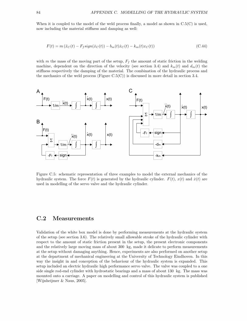
84 APPENDIX C. MODELLING OF THE HYDRAULIC SYSTEM
When it is coupled to the model of the weld process finally, a model as shown in C.5(C) is used,now including the material stiffness and damping as well:
F (t) = m (xC(t) − Ffsign(xC(t)) − bm(t)xC(t) − km(t)xC(t)) (C.44)
with m the mass of the moving part of the setup, Ff the amount of static friction in the weldingmachine, dependent on the direction of the velocity (see section 3.4) and km(t) and dm(t) thestiffness respectively the damping of the material. The combination of the hydraulic process andthe mechanics of the weld process (Figure C.5(C)) is discussed in more detail in section 3.4.
S 1/m ò
sign
ò
-Ff
-dm
-km
F(t)
x(t)1/m ò ò
F(t) x(t)
S1/m ò
sign
ò
-Ff
F(t)
x(t)
A
B
C.x(t)..
x(t)
.x(t)
.x(t)
..x(t)
..x(t)
Figure C.5: schematic representation of three examples to model the external mechanics of thehydraulic system. The force F (t) is generated by the hydraulic cylinder. F (t), x(t) and x(t) areused in modelling of the servo valve and the hydraulic cylinder.
C.2 Measurements
Validation of the white box model is done by performing measurements at the hydraulic systemof the setup (see section 3.6). The relatively small allowable stroke of the hydraulic cylinder withrespect to the amount of static friction present in the setup, the present electronic componentsand the relatively large moving mass of about 300 kg, made it delicate to perform measurementsat the setup without damaging anything. Hence, experiments are also performed on another setupat the department of mechanical engineering at the University of Technology Eindhoven. In thisway the insight in and conception of the behaviour of the hydraulic system is expanded. Thissetup included an electric hydraulic high performance servo valve. The valve was coupled to a oneside single rod-end cylinder with hydrostatic bearings and a mass of about 130 kg. The mass wasmounted onto a carriage. A paper on modelling and control of this hydraulic system is published[Wijnheijmer & Naus, 2005].

C.2. MEASUREMENTS 85
C HSc u
S
position or pressure
r e outS
w
Figure C.6: schematic representation of the measurement setup for performing sensitivity or directmeasurements to determine the transfer function of the hydraulic system HS with C a feedbackcontroller.
To examine the characteristics of the system, the frequency responses of the system are de-termined using two techniques. A closed loop setup as depicted in Figure C.6 is used to preventdrifting of the system. Because of this, a sensitivity measurement is preferable for the determina-tion of the position frequency response of the system. A direct measurement gives good resultsfor the determination of the pressure frequency response of the system. The disturbance signal win Figure C.6 is omitted in case of a direct measurement. The signal r is a reference signal, whichin case of a direct measurement consists of two parts. Firstly it has to be a signal with enoughfrequency content to determine the frequency response of the system H over a large frequencyrange, for example a white noise-alike signal. Secondly it consists of a prescribed trajectory, forexample a constant position or pressure, which prevents drifting of the system. The white noise-alike signal is added to this second reference signal. In case of a sensitivity measurement thedisturbance signal w in Figure C.6 fulfils this function and the reference signal only consists ofthe reference trajectory to prevent drifting of the system. Instead of a white noise-alike signal aso-called chirp signal may be used. This introduces an input signal with increasing and decreasingfrequency input in between a prescribed frequency range. Because of the integrating behaviourof the hydraulic system however, the magnitude of the chirp signal will decrease with increasingfrequencies. In combination with the relatively large amount of static friction present in the setupand the limited stroke of the rod of the hydraulic cylinder, it is difficult to keep the system injogging mode (moving) to overcome the static friction safe enough not to damage the setup. Somemeasurements using a chirp signal as input signal over a small frequency region are performed,especially in the frequency regions where a noise signal did not give good enough results. Theresults however were worse than those with a white noise-alike input signal. For the controllerC in Figure C.6 a small gain was used, which has to keep the system in the vicinity of the pre-scribed trajectory and therefore prevent drifting of the system. For this gain is compensated inthe calculations afterwards.
Using the direct measurement technique out and u are measured to determine the hydraulicsystem HS directly
HS =out
u(C.45)
with out the force F (t) or the displacement y(t). If the measured signals are transformed to thefrequency domain using a Laplace transformation, the transfer functions of the hydraulic systemHS result
HP =P
U(C.46)
Hy =Y
U(C.47)
Using the sensitivity measurement technique the sensitivity S of the system for a disturbance signalis measured from which the transfer functions of the system can be derived using the followingequations.
u = w + C(r − out) (C.48)

86 APPENDIX C. MODELLING OF THE HYDRAULIC SYSTEM
If a signal with only very small frequency content is chosen as a reference signal, the influence onthe output signal will be negligible with respect to the influence of the disturbance signal w andr may be neglected and equation C.48 becomes
u = w − Cout (C.49)
If the measured signals are transformed to the frequency domain using a Laplace transformationthe sensitivity S results
S =U
W(C.50)
= (1 + HC)−1 (C.51)
From this the system H can be calculated
H = C−1(S−1 − I) (C.52)
The results of the measurements are shown and discussed in section 3.6.3.
C.3 Black box modelling
The transfer functions resulting from the measurements can be used to fit a black box model ofthe system. From the white box modelling however some restrictions to the black box fit can bedetermined. Combining the model of the hydraulic system and the external mechanics of FigureC.5(C) leaving the friction out, a representation of the total mechanics of the weld process results.To gain better understanding in the frequency responses of the total model, they are derived usingthe white box model. In this way the two resulting frequency responses are deducted. The effectof an input signal to the servo valve on the resulting pressure pl(t) and the effect of the inputsignal on the resulting displacement y(t) are examined.
Summarising the pressure-based equations
Pn =pl
sps
(C.53)
pl =EoilL
L2
4 − y2(ql
A− y) (C.54)
ql = qnxn(1 − signxnpn) (C.55)
Combining these equations and rearranging the variables results in the following equation for thefrequency dependent pressure
Pn =EoilL(Xnqn − Y sA)
Asps(L2
4 − Y 2) + qn
2 signXnEoilL(C.56)
with Pn, Y and Xn the Laplace transformed frequency dependent variables based on pn(t), y(t)and xn(t).
The position-based equations are
Y =y
s(C.57)
y =
∑
F
s2m(C.58)
∑
F = pnA − ky − dy (C.59)
which results in the following equation for the frequency dependent position
Y =PnA
ms2 + ds + k(C.60)
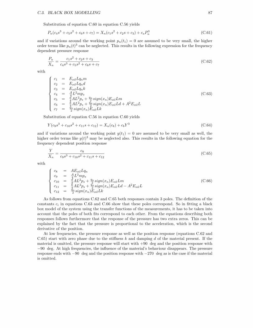
C.3. BLACK BOX MODELLING 87
Substitution of equation C.60 in equation C.56 yields
Pn(c4s3 + c5s
2 + c6s + c7) = Xn(c1s2 + c2s + c3) + caP 3
n (C.61)
and if variations around the working point pn(t1) = 0 are assumed to be very small, the higherorder terms like pn(t)3 can be neglected. This results in the following expression for the frequencydependent pressure response
Pn
Xn
=c1s
2 + c2s + c3
c4s3 + c5s2 + c6s + c7(C.62)
with
c1 = EoilLqnmc2 = EoilLqndc3 = EoilLqnkc4 = A
4 L2mps
c5 = d4AL2ps + qn
2 sign(xn)EoilLmc6 = k
4AL2ps + qn
2 sign(xn)EoilLd + A2EoilLc7 = qn
2 sign(xn)EoilLk
(C.63)
Substitution of equation C.56 in equation C.60 yields
Y (c9s3 + c10s
2 + c11s + c12) = Xn(c8) + cbY3 (C.64)
and if variations around the working point y(t1) = 0 are assumed to be very small as well, thehigher order terms like y(t)3 may be neglected also. This results in the following equation for thefrequency dependent position response
Y
Xn
=c8
c9s3 + c10s2 + c11s + c12(C.65)
with
c8 = AEoilLqn
c9 = A4 L2mps
c10 = d4AL2ps + qn
2 sign(xn)EoilLmc11 = k
4AL2ps + qn
2 sign(xn)EoilLd − A2EoilLc12 = qn
2 sign(xn)EoilLk
(C.66)
As follows from equations C.62 and C.65 both responses contain 3 poles. The definition of theconstants ci in equations C.63 and C.66 show that these poles correspond. So in fitting a blackbox model of the system using the transfer functions of the measurements, it has to be taken intoaccount that the poles of both fits correspond to each other. From the equations describing bothresponses follows furthermore that the response of the pressure has two extra zeros. This can beexplained by the fact that the pressure is proportional to the acceleration, which is the secondderivative of the position.
At low frequencies, the pressure response as well as the position response (equations C.62 andC.65) start with zero phase due to the stiffness k and damping d of the material present. If thematerial is omitted, the pressure response will start with +90 deg and the position response with−90 deg. At high frequencies, the influence of the material’s behaviour disappears. The pressureresponse ends with −90 deg and the position response with −270 deg as is the case if the materialis omitted.

88 APPENDIX C. MODELLING OF THE HYDRAULIC SYSTEM

Appendix D
Weld process model
An overview of the model of the weld process based on the model developed in Chapter 3 andthe assumptions made in section 4.3 is given in this Appendix. In the first section the nonlinearstate-space representation of the model is given. In section D.2 the transfer functions resultingfrom a linearisation of this model discussed in section 4.4.
D.1 Nonlinear state-space model
Defining the state vector x(t)
x(t) =
x1 = normalised spool valve position xn(t)x2 = velocity of the normalised spool valve movementxn(t)x3 = normalised pressure pn(t)x4 = welding seam temperature T (t)x5 = displacement of the right clamp y(t)x6 = velocity of the right clamp y(t)x7 = electrical current i(t)
x8 = time derivative of the electrical current i(t)
(D.1)
the input vector u(t)
u(t) =
[
u1 = inverter control signal ui(t)u2 = servo valve control signal uv(t)
]
(D.2)
and the output vector y(t)
y(t) =
y1 = displacement y(t)y2 = temperature T (t)y3 = normalised pressure pn(t)
(D.3)
The nonlinear state-space model of the weld process becomes
x(t) = f(x(t), u(t)) (D.4)
y(t) = g(x(t), u(t))
with
x(t) = f(x, u) (D.5)
89

90 APPENDIX D. WELD PROCESS MODEL
=
xn(t)xn(t)pn(t)
T (t)y(t)y(t)
i(t)
i(t)
The accompanying system of differential equations resulting from the modelling in Chapter 3 andthe assumptions made in section 4.3 are
x1 = x2
x2 = c1u2 + c2x2 + c3x1 (D.6)
x3 = c4ql
(
c5 + c6x25 + c7x6 + x6x
25 + c8x3 + c9x3x
25
)
−1
x4 = c10 (c11 + x5)−1 (
c12x27 + c13x5x
27 + c14x4x
27 + ...
+c15x4x5x27 + (Ty(t) + c17)
−1(
c16x27F (t)−1Ty(t) + ...
+c18x27F (t)−1x4Ty(t) + c19x
27F (t)−1x4 + c20x
27F (t)−1x2
4
)
+ ...
+c21x6x4 + c22(c10 + x5)−2 + c23(c10 + x5)
−2x5
+c24(c10 + x5)−2x4 + c25(c10 + x5)
−2x5x4
)
x5 = x6
x6 = c26F (t) + c27k(t)x5 + c27d(t)x6
x7 = x8
x8 = c28u1 + c29x8 + c30x7
with
F (t) = c31x3 (D.7)
k(t) =
kel for x4 ≤ Ty(t)0 for x4 > Ty(t)
(D.8)
d(t) =
del for x4 ≤ Ty(t)c32x
−14 + c33F (t)x−1
4 for x4 > Ty(t)(D.9)
Ty(t) = c34 + c35F (t) (D.10)
ql(t) = qn(c1 −x3
2sign(x1)) (D.11)
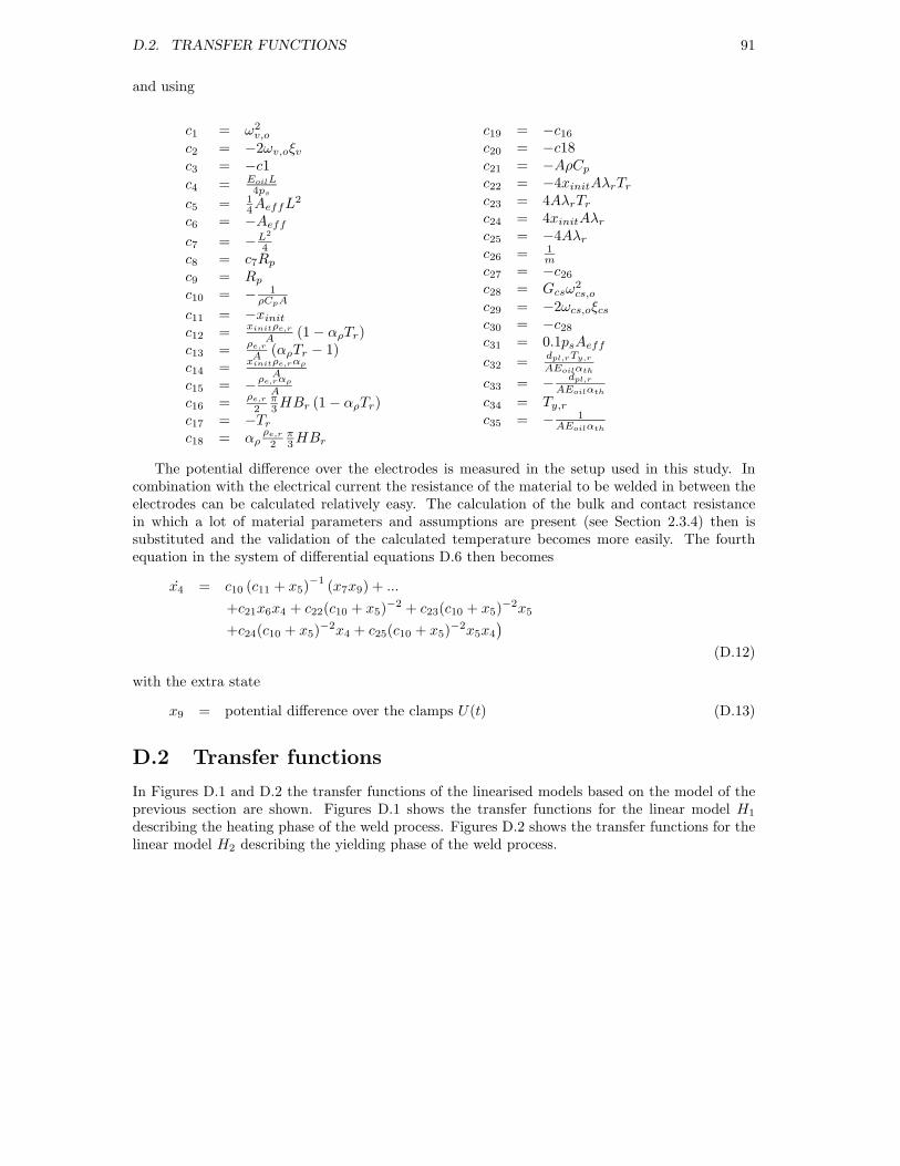
D.2. TRANSFER FUNCTIONS 91
and using
c1 = ω2v,o
c2 = −2ωv,oξv
c3 = −c1
c4 = EoilL4ps
c5 = 14AeffL2
c6 = −Aeff
c7 = −L2
4c8 = c7Rp
c9 = Rp
c10 = − 1ρCpA
c11 = −xinit
c12 =xinitρe,r
A(1 − αρTr)
c13 =ρe,r
A(αρTr − 1)
c14 =xinitρe,rαρ
A
c15 = −ρe,rαρ
A
c16 =ρe,r
2π3 HBr (1 − αρTr)
c17 = −Tr
c18 = αρρe,r
2π3 HBr
c19 = −c16
c20 = −c18c21 = −AρCp
c22 = −4xinitAλrTr
c23 = 4AλrTr
c24 = 4xinitAλr
c25 = −4Aλr
c26 = 1m
c27 = −c26
c28 = Gcsω2cs,o
c29 = −2ωcs,oξcs
c30 = −c28
c31 = 0.1psAeff
c32 =dpl,rTy,r
AEoilαth
c33 = −dpl,r
AEoilαth
c34 = Ty,r
c35 = − 1AEoilαth
The potential difference over the electrodes is measured in the setup used in this study. Incombination with the electrical current the resistance of the material to be welded in between theelectrodes can be calculated relatively easy. The calculation of the bulk and contact resistancein which a lot of material parameters and assumptions are present (see Section 2.3.4) then issubstituted and the validation of the calculated temperature becomes more easily. The fourthequation in the system of differential equations D.6 then becomes
x4 = c10 (c11 + x5)−1
(x7x9) + ...
+c21x6x4 + c22(c10 + x5)−2 + c23(c10 + x5)
−2x5
+c24(c10 + x5)−2x4 + c25(c10 + x5)
−2x5x4
)
(D.12)
with the extra state
x9 = potential difference over the clamps U(t) (D.13)
D.2 Transfer functions
In Figures D.1 and D.2 the transfer functions of the linearised models based on the model of theprevious section are shown. Figures D.1 shows the transfer functions for the linear model H1
describing the heating phase of the weld process. Figures D.2 shows the transfer functions for thelinear model H2 describing the yielding phase of the weld process.
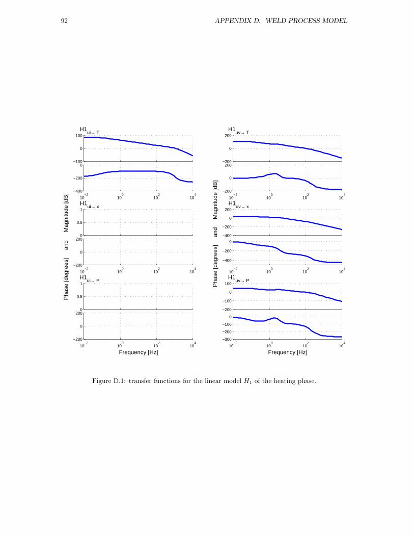
92 APPENDIX D. WELD PROCESS MODEL
−100
0
100H1
ui→ T
10−2
100
102
104
−400
−200
0
0
0.5
1H1
ui→ x
10−2
100
102
104
−200
0
200
0
0.5
1H1
ui→ P
10−2
100
102
104
−200
0
200
Frequency [Hz]
Pha
se [d
egre
es]
an
d
Mag
nitu
de [d
B]
−200
0
200H1
uv→ T
10−2
100
102
104
−200
0
200
−400
−200
0
200H1
uv→ x
10−2
100
102
104
−400
−200
0
−200
−100
0
100H1
uv→ P
10−2
100
102
104
−300
−200
−100
0
Frequency [Hz]
Pha
se [d
egre
es]
an
d
Mag
nitu
de [d
B]
Figure D.1: transfer functions for the linear model H1 of the heating phase.

D.2. TRANSFER FUNCTIONS 93
−100
0
100H2
ui→ T
10−2
100
102
104
−300
−200
−100
0
−400
−200
0
200H2
ui→ x
10−2
100
102
104
−400
−200
0
−300
−200
−100
0H2
ui→ P
10−2
100
102
104
−400
−200
0
Frequency [Hz]
Pha
se [d
egre
es]
an
d
Mag
nitu
de [d
B]
−200
−100
0
100H2
uv→ T
10−2
100
102
104
−200
0
200
−400
−200
0
200H2
uv→ x
10−2
100
102
104
−400
−200
0
−200
−100
0
100H2
uv→ P
10−2
100
102
104
−300
−200
−100
0
100
Frequency [Hz]
Pha
se [d
egre
es]
an
d
Mag
nitu
de [d
B]
Figure D.2: transfer functions for the linear model H2 of the yielding phase.

94 APPENDIX D. WELD PROCESS MODEL
Appendix E
MCDesign
Various tools like DIET (Do It Easy Tool) [DIET, 2003] and SISOtool which is a tool of the controlsystem toolbox of MatlabR13 exist for controller design using loop shaping techniques. Most ofthese tools are developed for controller design of SISO systems or models. For MIMO loop shapingno appropriate tool is at hands. Therefore MCDesign (MIMO Control Design) [MCDesign, 2005]was developed by G.J.L. Naus and F.P. Wijnheijmer to facilitate working with these systems andmodels.
MCDesign uses the MatlabR13 environment and consists of three main parts. The dtf-dataobject, which facilitates working with measurement data. Calculation with SISO as well as MIMOdata and models is reduced to summation, multiplication, et cetera of the dtf object. CDesign is atool to apply loop shaping and pole-zero placement techniques to SISO systems. Using CDesign,controllers can be designed as well as black box fits of measurement data can be made. MDesignis the command window controlling the data, especially suited for MIMO systems. In the mainwindow, the various transfer functions of the system are shown from where controllers, fits of thedata, et cetera can be designed. To simplify importing measurement data into MDesign, SDesignis developed. SDesign is a tool to convert measurement input output data to data-based transferfunctions, which can be imported into MDesign. In the near future among other things, alsoMIMO system data fitting, which signifies ’grey’ box fitting with fixed poles as well as H∞ controlwill be implemented.
For a thorough description of the MCDesign tool, see the MCDesign Manual [MCDesign man-ual, 2005].
95

96 APPENDIX E. MCDESIGN
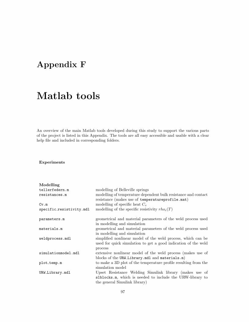
Appendix F
Matlab tools
An overview of the main Matlab tools developed during this study to support the various partsof the project is listed in this Appendix. The tools are all easy accessible and usable with a clearhelp file and included in corresponding folders.
Experiments
Modellingtellerfedern.m modelling of Belleville springsresistances.m modelling of temperature dependent bulk resistance and contact
resistance (makes use of temperatureprofile.mat)Cv.m modelling of specific heat Cv
specific resistivity.mdl modelling of the specific resistivity rhoe(T )
parameters.m geometrical and material parameters of the weld process usedin modelling and simulation
materials.m geometrical and material parameters of the weld process usedin modelling and simulation
weldprocess.mdl simplified nonlinear model of the weld process, which can beused for quick simulation to get a good indication of the weldprocess
simulationmodel.mdl extensive nonlinear model of the weld process (makes use ofblocks of the URW Library.mdl and materials.m)
plot temp.m to make a 3D plot of the temperature profile resulting from thesimulation model
URW Library.mdl Upset Resistance Welding Simulink library (makes use ofslblocks.m, which is needed to include the URW-library tothe general Simulink library)
97
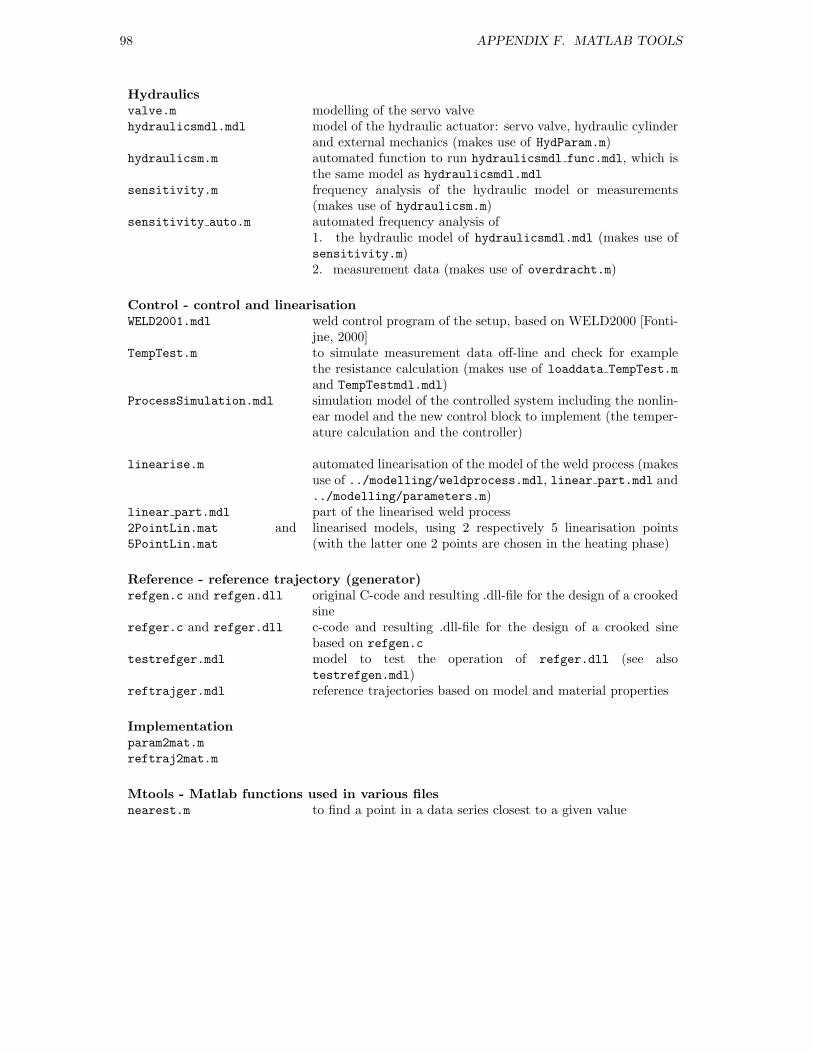
98 APPENDIX F. MATLAB TOOLS
Hydraulicsvalve.m modelling of the servo valvehydraulicsmdl.mdl model of the hydraulic actuator: servo valve, hydraulic cylinder
and external mechanics (makes use of HydParam.m)hydraulicsm.m automated function to run hydraulicsmdl func.mdl, which is
the same model as hydraulicsmdl.mdlsensitivity.m frequency analysis of the hydraulic model or measurements
(makes use of hydraulicsm.m)sensitivity auto.m automated frequency analysis of
1. the hydraulic model of hydraulicsmdl.mdl (makes use ofsensitivity.m)2. measurement data (makes use of overdracht.m)
Control - control and linearisationWELD2001.mdl weld control program of the setup, based on WELD2000 [Fonti-
jne, 2000]TempTest.m to simulate measurement data off-line and check for example
the resistance calculation (makes use of loaddata TempTest.m
and TempTestmdl.mdl)ProcessSimulation.mdl simulation model of the controlled system including the nonlin-
ear model and the new control block to implement (the temper-ature calculation and the controller)
linearise.m automated linearisation of the model of the weld process (makesuse of ../modelling/weldprocess.mdl, linear part.mdl and../modelling/parameters.m)
linear part.mdl part of the linearised weld process2PointLin.mat and5PointLin.mat
linearised models, using 2 respectively 5 linearisation points(with the latter one 2 points are chosen in the heating phase)
Reference - reference trajectory (generator)refgen.c and refgen.dll original C-code and resulting .dll-file for the design of a crooked
sinerefger.c and refger.dll c-code and resulting .dll-file for the design of a crooked sine
based on refgen.c
testrefger.mdl model to test the operation of refger.dll (see alsotestrefgen.mdl)
reftrajger.mdl reference trajectories based on model and material properties
Implementationparam2mat.m
reftraj2mat.m
Mtools - Matlab functions used in various filesnearest.m to find a point in a data series closest to a given value