Massachusetts Institute of TechnologyDepartment of Electrical Engineering and Computer Science

6.061 Introduction to Power SystemsClass Notes Chapter 11

DC (Commutator) and Permanent Magnet Machines ∗

J.L. Kirtley Jr.

1 Introduction

Virtually all electric machines, and all practical electric machines employ some form of rotating or alternating field/current system to produce torque. While it is possible to produce a “true DC” machine (e.g. the “Faraday Disk”), for practical reasons such machines have not reached application and are not likely to. In the machines we have examined so far the machine is operated from an alternating voltage source. Indeed, this is one of the principal reasons for employing AC in power systems.

The first electric machines employed a mechanical switch, in the form of a carbon brush/commutator system, to produce this rotating field. While the widespread use of power electronics is making “brushless” motors (which are really just synchronous machines) more popular and common, com­mutator machines are still economically very important. They are relatively cheap, particularly in small sizes, they tend to be rugged and simple.

You will find commutator machines in a very wide range of applications. The starting motor on all automobiles is a series-connected commutator machine. Many of the other electric motors in automobiles, from the little motors that drive the outside rear-view mirrors to the motors that drive the windshield wipers are permanent magnet commutator machines. The large traction motors that drive subway trains and diesel/electric locomotives are DC commutator machines (although induction machines are making some inroads here). And many common appliances use “universal” motors: series connected commutator motors adapted to AC.

1.1 Geometry:

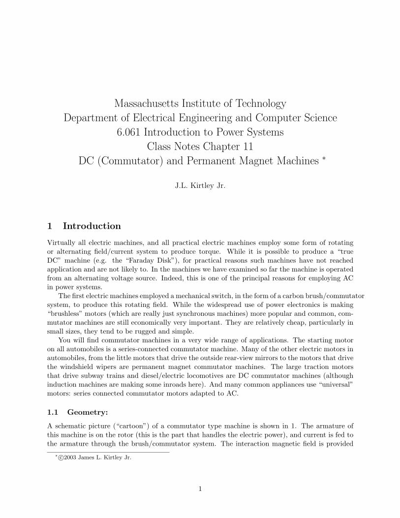
A schematic picture (“cartoon”) of a commutator type machine is shown in 1. The armature of this machine is on the rotor (this is the part that handles the electric power), and current is fed to the armature through the brush/commutator system. The interaction magnetic field is provided

∗ c�2003 James L. Kirtley Jr.

1

Stator Yoke Field Poles

Field Winding

Armature Winding

Rotor Ω

Figure 1: Wound-Field DC Machine Geometry

(in this picture) by a field winding. A permanent magnet field is applicable here, and we will have quite a lot more to say about such arrangements below.

Now, if we assume that the interaction magnetic flux density averages Br, and if there are Ca

conductors underneath the poles at any one time, and if there are m parallel paths, then we may estimate torque produced by the machine by:

Ca R�BrIaTe =

m

where R and � are rotor radius and length, respectively and Ia is terminal current. Note that Ca

is not necessarily the total number of conductors, but rather the total number of active conductors (that is, conductors underneath the pole and therefore subject to the interaction field). Now, if we note Nf as the number of field turns per pole, the interaction field is just:

NfIfBr =

g

leading to a simple expression for torque in terms of the two currents:

Te = GIaIf

where G is now the motor coefficient (units of N-m/ampere squared):

Ca NfG = µ0 R�

m g

Now, let’s go back and look at this from the point of view of voltage. Start with Faraday’s Law:

∂B��× E� = −

∂t

Integrating both sides and noting that the area integral of a curl is the edge integral of the quantity, we find:

� ��

∂B�E� · d� = −

∂t

2

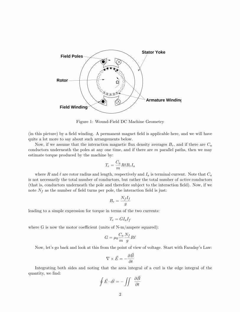
Now, that is a bit awkward to use, particularly in the case we have here in which the edge of the contour is moving (note we will be using this expression to find voltage). We can make this a bit more convenient to use if we note:

where v' is the velocity of the contour. This gives us a convenient way of noting the apparent electric field within a moving object (as in the conductors in a DC machine):

Figure 2: Motion of a contour through a magnetic field produces flux change and electric field in the moving contour

Now, note that the armature conductors are moving through the magnetic field produced by the stator (field) poles, and we can ascribe to them an axially directed electric field:

If the armature conductors are arranged as described above, with Ca conductors in m parallel paths underneath the poles and with a mean active radial magnetic field of B,, we can compute a voltage induced in the stator conductors:

Note that this is only the voltage induced by motion of the armature conductors through the field and does not include brush or conductor resistance. If we include the expression for effective magnetic field, we find that the back voltage is:

which leads us to the conclusion that newton-meters per ampere squared equals volt seconds per ampere. This stands to reason if we examine electric power into the interaction and mechanical power out:

Pe, = EbIa=TeR

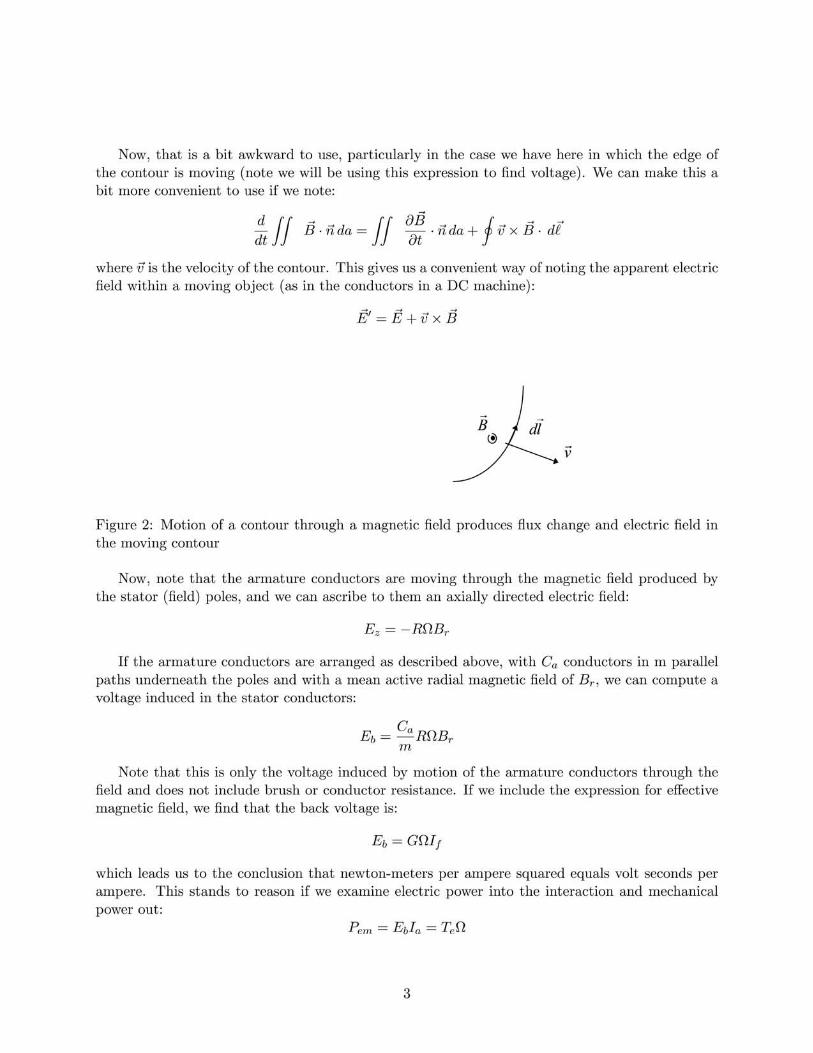
Now, a more complete model of this machine would include the effects of armature, brush and lead resistance, so that in steady state operation:

Va = RaIa + GΩIf

Now, consider this machine with its armatucre connected to a voltage source and its field operating at steady current, so that:

Va −GΩIfIa =

Ra

G I fΩ +

Va

-

Ra

+

-

Figure 3: DC Machine Equivalent Circuit

Then torque, electric power in and mechanical power out are:

Te = GIf

Va −GΩIf

Ra

Pe = Va

Va −GΩIf

Ra

Pm = GΩIf

Va −GΩIf

Ra

Now, note that these expressions define three regimes defined by rotational speed. The two “break points” are at zero speed and at the “zero torque” speed:

VaΩ0 =

GIf

For 0 < Ω < Ω0, the machine is a motor: electric power in and mechanical power out are both positive. For higher speeds: Ω0 < Ω , the machine is a generator, with electrical power in and mechanical power out being both negative. For speeds less than zero, electrical power in is positive and mechanical power out is negative. There are few needs to operate machines in this regime, short of some types of ”plugging” or emergency braking in tractions systems.

1.2 Hookups:

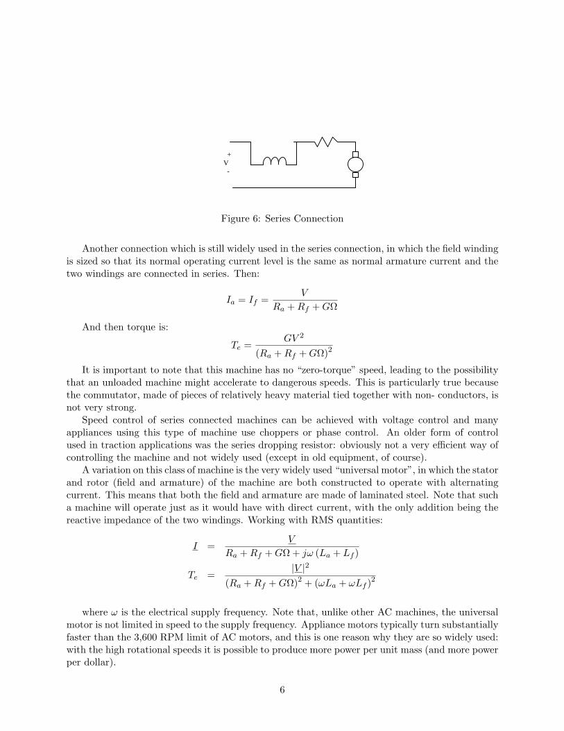
We have just described a mode of operation of a commutator machine usually called “separately excited”, in which field and armature circuits are controlled separately. This mode of operation is used in some types of traction applications in which the flexibility it affords is useful. For example,

4

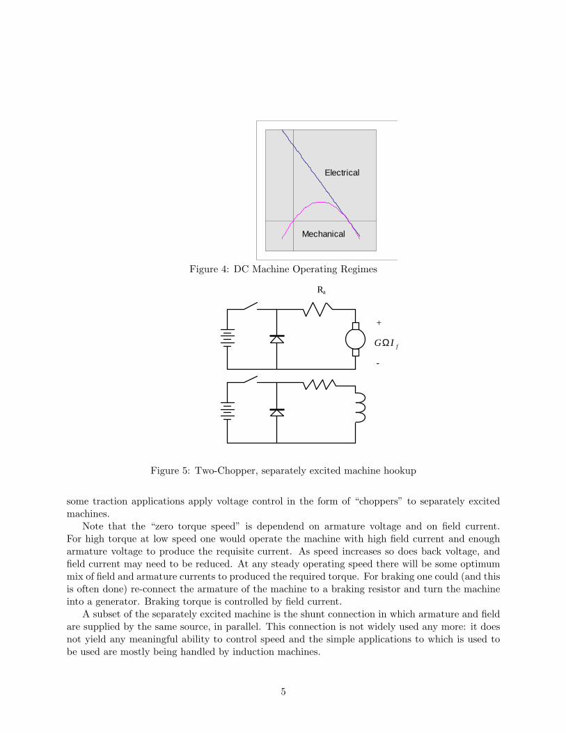
Mechanical

Electrical

Figure 4: DC Machine Operating Regimes

G I fΩ

Ra

+

-

Figure 5: Two-Chopper, separately excited machine hookup

some traction applications apply voltage control in the form of “choppers” to separately excited machines.

Note that the “zero torque speed” is dependend on armature voltage and on field current. For high torque at low speed one would operate the machine with high field current and enough armature voltage to produce the requisite current. As speed increases so does back voltage, and field current may need to be reduced. At any steady operating speed there will be some optimum mix of field and armature currents to produced the required torque. For braking one could (and this is often done) re-connect the armature of the machine to a braking resistor and turn the machine into a generator. Braking torque is controlled by field current.

A subset of the separately excited machine is the shunt connection in which armature and field are supplied by the same source, in parallel. This connection is not widely used any more: it does not yield any meaningful ability to control speed and the simple applications to which is used to be used are mostly being handled by induction machines.

5

+ V

­

Figure 6: Series Connection

Another connection which is still widely used in the series connection, in which the field winding is sized so that its normal operating current level is the same as normal armature current and the two windings are connected in series. Then:

V Ia = If =

Ra + Rf + GΩ

And then torque is: GV 2

Te = (Ra + Rf + GΩ)2

It is important to note that this machine has no “zero-torque” speed, leading to the possibility that an unloaded machine might accelerate to dangerous speeds. This is particularly true because the commutator, made of pieces of relatively heavy material tied together with non- conductors, is not very strong.

Speed control of series connected machines can be achieved with voltage control and many appliances using this type of machine use choppers or phase control. An older form of control used in traction applications was the series dropping resistor: obviously not a very efficient way of controlling the machine and not widely used (except in old equipment, of course).

A variation on this class of machine is the very widely used “universal motor”, in which the stator and rotor (field and armature) of the machine are both constructed to operate with alternating current. This means that both the field and armature are made of laminated steel. Note that such a machine will operate just as it would have with direct current, with the only addition being the reactive impedance of the two windings. Working with RMS quantities:

V I =

Ra + Rf + GΩ + jω (La + Lf )

|V |2

Te = (Ra + Rf + GΩ)2 + (ωLa + ωLf )2

where ω is the electrical supply frequency. Note that, unlike other AC machines, the universal motor is not limited in speed to the supply frequency. Appliance motors typically turn substantially faster than the 3,600 RPM limit of AC motors, and this is one reason why they are so widely used: with the high rotational speeds it is possible to produce more power per unit mass (and more power per dollar).

6

1.3 Commutator:

The commutator is what makes this machine work. The brush and commutator system of this class of motor involves quite a lot of “black art”, and there are still aspects of how they work which are poorly understood. However, we can make some attempt to show a bit of what the brush/commutator system does.

To start, take a look at the picture shown in Figure 7. Represented are a pair of poles (shaded) and a pair of brushes. Conductors make a group of closed paths. Current from one of the brushes takes two parallel paths. You can follow one of those paths around a closed loop, under each of the two poles (remember that the poles are of opposite polarity) to the opposite brush. Open commutator segments (most of them) do not carry current into or out of the machine.

Figure 7: Commutator and Current Paths

A commutation interval occurs when the current in one coil must be reversed. (See Figure 8 In the simplest form this involves a brush bridging between two commutator segments, shorting out that coil. The resistance of the brush causes the current to decay. When the brush leaves the leading segment the current in the leading coil must reverse.

Figure 8: Commutator at Commutation

We will not attempt to fully understand the commutation process in this type of machine, but we can note a few things. Resistive commutation is the process relied upon in small machines.

7

When the current in one coil must be reversed (because it has left one pole and is approaching the other), that coil is shorted by one of the brushes. The brush resistance causes the current in the coil to decay. Then the leading commutator segment leaves the brush the current MUST reverse (the trailing coil has current in it), and there is often sparking.

1.4 Commutation

Commutation

Stator Yoke Field Poles

Field Winding

Armature Winding

Rotor Ω

Interpoles

Figure 9: Commutation Interpoles

In larger machines the commutation process would involve too much sparking, which causes brush wear, noxious gases (ozone) that promote corrosion, etc. In these cases it is common to use separate commutation interpoles. These are separate, usually narrow or seemingly vestigal pole pieces which carry armature current. They are arranged in such a way that the flux from the interpole drives current in the commutated coil in the proper direction. Remember that the coil being commutated is located physically between the active poles and the interpole is therefore in the right spot to influence commutation. The interpole is wound with armature current (it is in series with the main brushes). It is easy to see that the interpole must have a flux density proportional to the current to be commutated. Since the speed with which the coil must be commutated is proportional to rotational velocity and so is the voltage induced by the interpole, if the right number of turns are put around the interpole, commutation can be made to be quite accurate.

1.5 Compensation:

The analysis of commutator machines often ignores armature reaction flux. Obviously these ma­chines DO produce armature reaction flux, in quadrature with the main field. Normally, commuta­tor machines are highly salient and the quadrature inductance is lower than direct-axis inductance, but there is still flux produced. This adds to the flux density on one side of the main poles (pos­sibly leading to saturation). To make the flux distribution more uniform and therefore to avoid this saturation effect of quadrature axis flux, it is common in very highly rated machines to wind compensation coils: essentially mirror-images of the armature coils, but this time wound in slots in the surface of the field poles. Such coils will have the same number of ampere-turns as the

8

2

Rotor

Commutation Interpoles

Pole−Face Compensation Winding

Field Poles

Field Winding

Armature Winding

Ω

Figure 10: Pole Face Compensation Winding

armature. Normally they have the same number of turns and are connected directly in series with the armature brushes. What they do is to almost exactly cancel the flux produced by the armature coils, leaving only the main flux produced by the field winding. One might think of these coils as providing a reaction torque, produced in exactly the same way as main torque is produced by the armature. A cartoon view of this is shown in Figure 10.

Permanent Magnets in Electric Machines

Of all changes in materials technology over the last several years, advances in permanent magnets have had the largest impact on electric machines. Permanent magnets are often suitable as replace­ments for the field windings in machines: that is they can produce the fundamental interaction field. This does three things. First, since the permanent magnet is lossless it eliminates the energy required for excitation, usually improving the efficiency of the machine. Second, since eliminating the excitation loss reduces the heat load it is often possible to make PM machines more compact. Finally, and less appreciated, is the fact that modern permanent magnets have very large coercive force densities which permit vastly larger air gaps than conventional field windings, and this in turn permits design flexibility which can result in even better electric machines.

These advantages come not without cost. Permanent magnet materials have special character­istics which must be taken into account in machine design. The highest performance permanent magnets are brittle ceramics, some have chemical sensitivities, all are sensitive to high temperatures, most have sensitivity to demagnetizing fields, and proper machine design requires understanding the materials well. These notes will not make you into seasoned permanent magnet machine de­signers. They are, however, an attempt to get started, to develop some of the mathematical skills

9

required and to point to some of the important issues involved.

2.1 Permanent Magnets:

Hysteresis Loop: Perm anent Magn et

-1

-0.8

-0.6

-0.4

-0.2

0

0.2

0.4

0.6

0.8

1

-400 -300 -200 -100 0 100 200 300 400

Kilo Am per es /Meter

Tes

la

Figure 11: Hysteresis Loop Of Ceramic Permanent Magnet

Permanent magnet materials are, at core, just materials with very wide hysteresis loops. Fig­ure 11 is an example of something close to one of the more popular ceramic magnet materials.Note that this hysteresis loop is so wide that you can see the effect of the permeability of free space.

Figure 12: Demagnetization Curve

It is usual to display only part of the magnetic characteristic of permanent magnet materials (see Figure 12), the third quadrant of this picture, because that is where the material is normally

10

Demagnetization Curve

0

0.05

0.1

0.15

0.2

0.25

0.3

0.35

0.4

0.45

0.5

-250 -200 -150 -100 -50 0

H, kA/m

B, T

esla

BrEnergy Product Loci

Hc

�

operated. Note a few important characteristics of what is called the “demagnetization curve”. The remanent flux density Br, is the value of flux density in the material with zero magnetic field H. The coercive field Hc is the magnetic field at which the flux density falls to zero. Shown also on the curve are loci of constant energy product. This quantity is unfortunately named, for although it has the same units as energy it represents real energy in only a fairly general sense. It is the product of flux density and field intensity. As you already know, there are three commonly used systems of units for magnetic field quantities, and these systems are often mixed up to form very confusing units. We will try to stay away from the English system of units in which field intensity H is measured in amperes per inch and flux density B in lines (actually, usually kilolines) per square inch. In CGS units flux density is measured in Gauss (or kilogauss) and magnetic field intensity in Oersteds. And in SI the unit of flux density is the Tesla, which is one Weber per square meter, and the unit of field intensity is the Ampere per meter. Of these, only the last one, A/m is obvious. A Weber is a volt-second. A Gauss is 10−4 Tesla. And, finally, an Oersted is that field intensity required to produce one Gauss in the permeability of free space. Since the permeability of free space µ0 = 4π × 10−7Hy/m, this means that one Oe is about 79.58 A/m. Commonly, the energy product is cited in MgOe (Mega-Gauss-Oersted)s. One MgOe is equal to 7.958kJ/m3 . A commonly used measure for the performance of a permanent magnet material is the maximum energy product, the largest value of this product along the demagnetization curve.

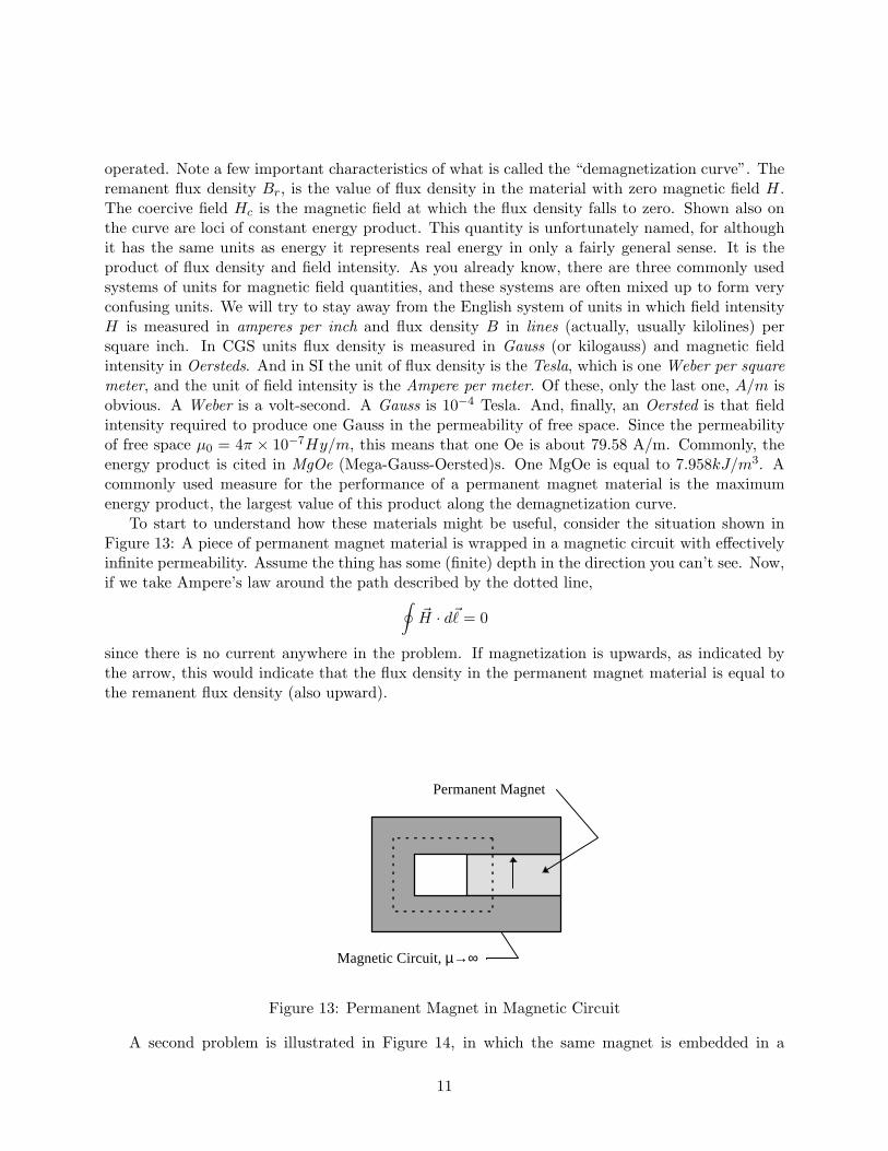
To start to understand how these materials might be useful, consider the situation shown in Figure 13: A piece of permanent magnet material is wrapped in a magnetic circuit with effectively infinite permeability. Assume the thing has some (finite) depth in the direction you can’t see. Now, if we take Ampere’s law around the path described by the dotted line,

H� · d�� = 0

since there is no current anywhere in the problem. If magnetization is upwards, as indicated by the arrow, this would indicate that the flux density in the permanent magnet material is equal to the remanent flux density (also upward).

Magnetic Circuit, µ→∞

Permanent Magnet

Figure 13: Permanent Magnet in Magnetic Circuit

A second problem is illustrated in Figure 14, in which the same magnet is embedded in a

11

��

� �

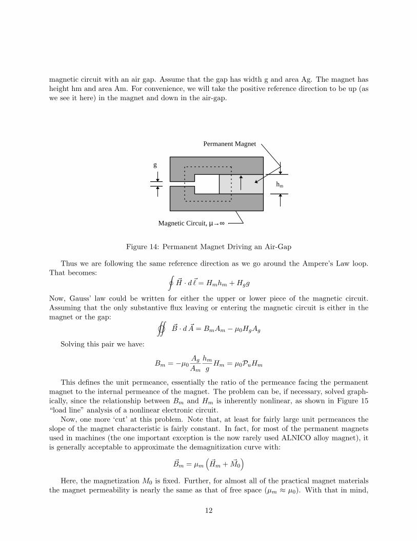
magnetic circuit with an air gap. Assume that the gap has width g and area Ag. The magnet has height hm and area Am. For convenience, we will take the positive reference direction to be up (as we see it here) in the magnet and down in the air-gap.

Magnetic Circuit, µ→∞

Permanent Magnet

g

hm

Figure 14: Permanent Magnet Driving an Air-Gap

Thus we are following the same reference direction as we go around the Ampere’s Law loop. That becomes:

�

H� · d �� = Hmhm + Hgg

Now, Gauss’ law could be written for either the upper or lower piece of the magnetic circuit. Assuming that the only substantive flux leaving or entering the magnetic circuit is either in the magnet or the gap:

� B� · dA� = BmAm − µ0HgAg

Solving this pair we have:

Ag hmBm = −µ0 Hm = µ0PuHm

Am g

This defines the unit permeance, essentially the ratio of the permeance facing the permanent magnet to the internal permeance of the magnet. The problem can be, if necessary, solved graph­ically, since the relationship between Bm and Hm is inherently nonlinear, as shown in Figure 15 “load line” analysis of a nonlinear electronic circuit.

Now, one more ‘cut’ at this problem. Note that, at least for fairly large unit permeances the slope of the magnet characteristic is fairly constant. In fact, for most of the permanent magnets used in machines (the one important exception is the now rarely used ALNICO alloy magnet), it is generally acceptable to approximate the demagnitization curve with:

B�m = µm H�m + M� 0

Here, the magnetization M0 is fixed. Further, for almost all of the practical magnet materials the magnet permeability is nearly the same as that of free space (µm ≈ µ0). With that in mind,

12

� �

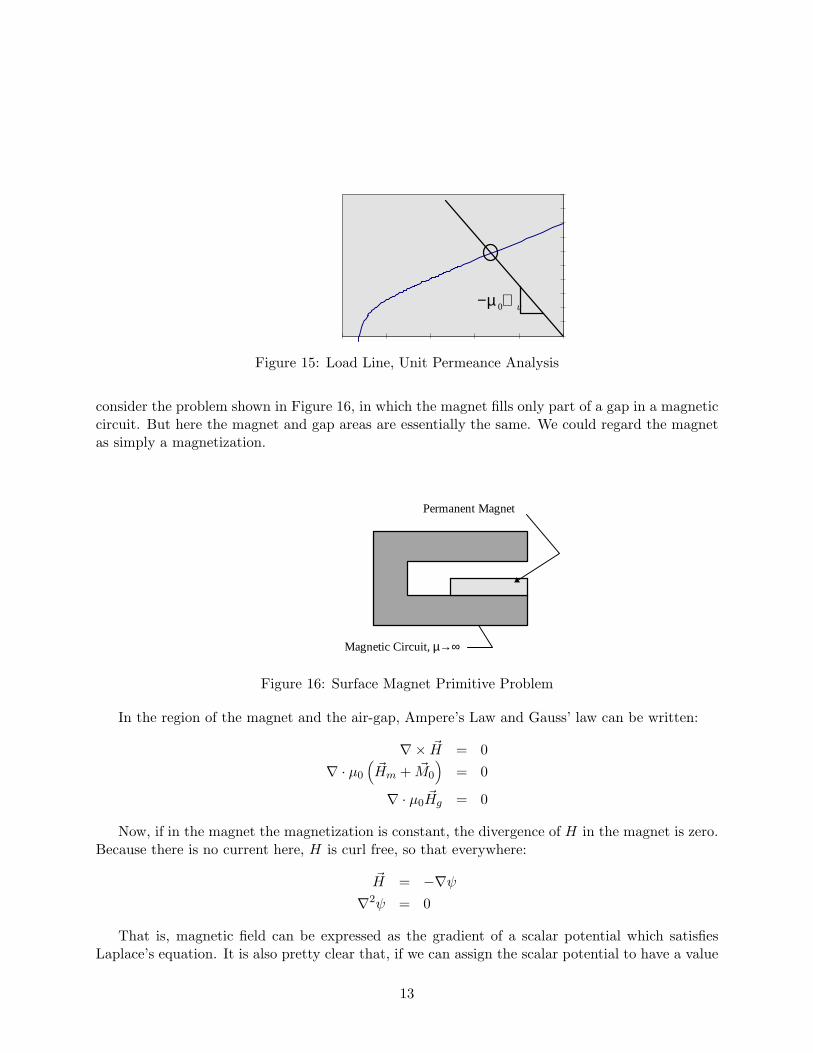
− ℘µ 0 u

Figure 15: Load Line, Unit Permeance Analysis

consider the problem shown in Figure 16, in which the magnet fills only part of a gap in a magnetic circuit. But here the magnet and gap areas are essentially the same. We could regard the magnet as simply a magnetization.

Permanent Magnet

Magnetic Circuit, µ→∞

Figure 16: Surface Magnet Primitive Problem

In the region of the magnet and the air-gap, Ampere’s Law and Gauss’ law can be written:

�× H� = 0

� · µ0 H�m + M� 0 = 0

� · µ0H� g = 0

Now, if in the magnet the magnetization is constant, the divergence of H in the magnet is zero. Because there is no current here, H is curl free, so that everywhere:

H� = −�ψ

�2ψ = 0

That is, magnetic field can be expressed as the gradient of a scalar potential which satisfies Laplace’s equation. It is also pretty clear that, if we can assign the scalar potential to have a value

13

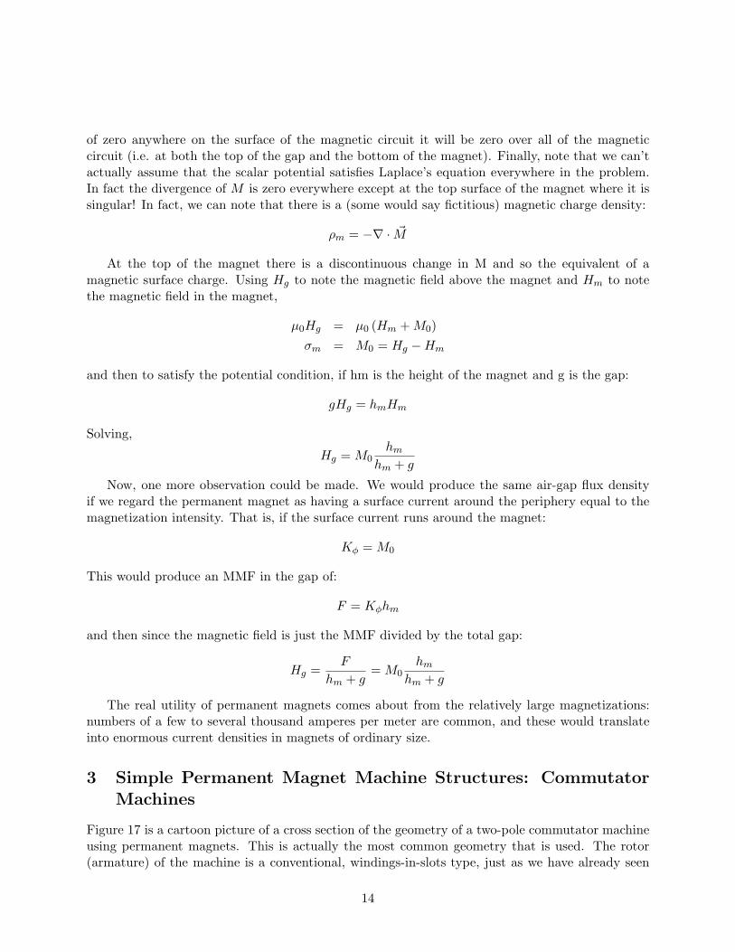
of zero anywhere on the surface of the magnetic circuit it will be zero over all of the magnetic circuit (i.e. at both the top of the gap and the bottom of the magnet). Finally, note that we can’t actually assume that the scalar potential satisfies Laplace’s equation everywhere in the problem. In fact the divergence of M is zero everywhere except at the top surface of the magnet where it is singular! In fact, we can note that there is a (some would say fictitious) magnetic charge density:

ρm = −� · M�

At the top of the magnet there is a discontinuous change in M and so the equivalent of a magnetic surface charge. Using Hg to note the magnetic field above the magnet and Hm to note the magnetic field in the magnet,

µ0Hg = µ0 (Hm + M0)

σm = M0 = Hg −Hm

and then to satisfy the potential condition, if hm is the height of the magnet and g is the gap:

gHg = hmHm

Solving, hm

Hg = M0 hm + g

Now, one more observation could be made. We would produce the same air-gap flux density if we regard the permanent magnet as having a surface current around the periphery equal to the magnetization intensity. That is, if the surface current runs around the magnet:

Kφ = M0

This would produce an MMF in the gap of:

F = Kφhm

and then since the magnetic field is just the MMF divided by the total gap:

F hmHg = = M0

hm + g hm + g

The real utility of permanent magnets comes about from the relatively large magnetizations: numbers of a few to several thousand amperes per meter are common, and these would translate into enormous current densities in magnets of ordinary size.

Simple Permanent Magnet Machine Structures: Commutator Machines

Figure 17 is a cartoon picture of a cross section of the geometry of a two-pole commutator machine using permanent magnets. This is actually the most common geometry that is used. The rotor (armature) of the machine is a conventional, windings-in-slots type, just as we have already seen

14

3

Field Magnets

Ω

Stator Yoke

Armature Winding

Rotor

Figure 17: PM Commutator Machine

for commutator machines. The field magnets are fastened (often just bonded) to the inside of a steel tube that serves as the magnetic flux return path.

Assume for the purpose of first-order analysis of this thing that the magnet is describable by its remanent flux density Br and had permeability of µ0. First, we will estimate the useful magnetic flux density and then will deal with voltage generated in the armature. Interaction Flux Density Using the basics of the analysis presented above, we may estimate the radial magnetic flux density at the air-gap as being:

BrBd =

1 + 1 Pc

where the effective unit permeance is:

fl hm AgPc =

ff g Am

A book on this topic by James Ireland suggests values for the two “fudge factors”:

1. The “leakage factor” fl is cited as being about 1.1.

2. The “reluctance factor” ff is cites as being about 1.2.

We may further estimate the ratio of areas of the gap and magnet by:

Ag R + g 2=

Am R + g + h2 m

Now, there are a bunch of approximations and hand wavings in this expression, but it seems to work, at least for the kind of machines contemplated.

A second correction is required to correct the effective length for electrical interaction. The reason for this is that the magnets produce fringing fields, as if they were longer than the actual

15

� �

”stack length” of the rotor (sometimes they actually are). This is purely empirical, and Ireland gives a value for effective length for voltage generation of:

�∗ �eff =

f�

where �∗ = � + 2NR , and the empirical coefficient

A hmN ≈ log 1 +B

B R

where

hmB = 7.4 − 9.0

R A = 0.9

3.0.1 Voltage:

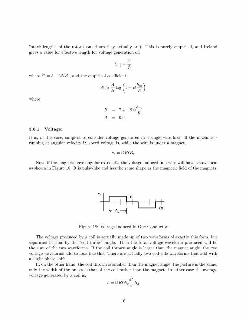
It is, in this case, simplest to consider voltage generated in a single wire first. If the machine is running at angular velocity Ω, speed voltage is, while the wire is under a magnet,

vs = ΩR�Br

Now, if the magnets have angular extent θm the voltage induced in a wire will have a waveform as shown in Figure 18: It is pulse-like and has the same shape as the magnetic field of the magnets.

θm

πvs

Ωt

Figure 18: Voltage Induced in One Conductor

The voltage produced by a coil is actually made up of two waveforms of exactly this form, but separated in time by the ”coil throw” angle. Then the total voltage waveform produced will be the sum of the two waveforms. If the coil thrown angle is larger than the magnet angle, the two voltage waveforms add to look like this: There are actually two coil-side waveforms that add with a slight phase shift.

If, on the other hand, the coil thrown is smaller than the magnet angle, the picture is the same, only the width of the pulses is that of the coil rather than the magnet. In either case the average voltage generated by a coil is:

θ∗ v = ΩR�Ns Bd

π

16

vc

0m

0m

Figure 19: Voltage Induced in a Coil

where θ∗ is the lesser of the coil throw or magnet angles and Ns is the number of series turns in the coil. This gives us the opportunity to develop the number of “active” turns:

Ca = Ns

θ∗ Ctot θ∗

= m π m π

Here, Ca is the number of active conductors, Ctot is the total number of conductors and m is the number of parallel paths. The motor coefficient is then:

R�effCtotBd θ∗ K =

m π

3.1 Armature Resistance

The last element we need for first-order prediction of performance of the motor is the value of armature resistance. The armature resistance is simply determined by the length and area of the wire and by the number of parallel paths (generally equal to 2 for small commutator motors). If we note Nc as the number of coils and Na as the number of turns per coil,

NcNaNs =

m

Total armature resistance is given by:

NsRa = 2ρw�t

m

where ρw is the resistivity (per unit length) of the wire:

1 ρw = πd2 σw4 w

(dw is wire diameter, σw is wire conductivity and �t is length of one half-turn). This length depends on how the machine is wound, but a good first-order guess might be something like this:

�t ≈ � + πR

17

MIT OpenCourseWarehttp://ocw.mit.edu

6.061 / 6.690 Introduction to Electric Power SystemsSpring 2011

For information about citing these materials or our Terms of Use, visit: http://ocw.mit.edu/terms.