Daytime D region parameters from long‐path VLF phaseand amplitude

Neil R. Thomson,1 Craig J. Rodger,1 and Mark A. Clilverd2

Received 5 June 2011; revised 2 August 2011; accepted 11 August 2011; published 2 November 2011.

[1] Observed phases and amplitudes of VLF radio signals propagating on very long pathsare used to validate electron density parameters for the lowest edge of the (D region of the)Earth’s ionosphere at low latitudes and midlatitudes near solar minimum. The phases,relative to GPS 1 s pulses, and the amplitudes were measured near the transmitters(∼100–150 km away), where the direct ground wave is dominant, and also at distancesof ∼8–14 Mm away, over mainly all‐sea paths. Four paths were used: NWC (19.8 kHz,North West Cape, Australia) to Seattle (∼14 Mm) and Hawaii (∼10 Mm), NPM (21.4 kHz,Hawaii) and NLK (24.8 kHz, Seattle) to Dunedin, New Zealand (∼8 Mm and ∼12 Mm).The characteristics of the bottom edge of the daytime ionosphere on these long pathswere found to confirm and contextualize recently measured short‐path values of Wait’straditional height and sharpness parameters, H′ and b, respectively, after adjustingappropriately for the (small) variations of H′ and b along the paths that are due to(1) changing solar zenith angles, (2) increasing cosmic ray fluxes with latitude, and(3) latitudinal and seasonal changes in neutral atmospheric densities from the (NASA)Mass Spectrometer Incoherent Scatter‐ (MSIS‐) E‐90 neutral atmosphere model.The sensitivity of this long‐path (and hence near‐global) phase and amplitude technique is∼ ± 0.3 km for H′ and ∼ ± 0.01 km−1 for b, thus creating the possibility of treating theheight (H′ ∼70 km) as a fiduciary mark (for a specified neutral density) in the Earth’satmosphere for monitoring integrated long‐term (climate) changes below ∼70 km altitude.

Citation: Thomson, N. R., C. J. Rodger, and M. A. Clilverd (2011), Daytime D region parameters from long‐path VLF phaseand amplitude, J. Geophys. Res., 116, A11305, doi:10.1029/2011JA016910.

1. Introduction

[2] The lowest altitude part of the Earth’s ionosphere is theD region. In this region the neutral atmosphere is ionizedmainly by solar EUV radiation and galactic cosmic rays. Lowin the D region, the downgoing solar EUV radiation isincreasingly absorbed by the increasing atmospheric density;also the electron attachment and recombination rates becomeso high that the free electron density becomes very small. Thelower D region (∼50–75 km) forms the rather stable upperboundary, or ceiling, of the Earth‐ionosphere waveguidewhile the oceans and the ground form the lower boundary.Very low frequency (VLF) radio waves (∼3–30 kHz) travelover the Earth’s surface in this waveguide. Observations ofthe propagation parameters of these waves result in one of thebest probes available for characterizing the height andsharpness of the lower D region. The (partial) ionosphericreflections of the VLF waves occur because the electrondensities (and hence refractive indices) change rapidly (in thespace of a wavelength) with height in this region (∼50–75 km)

typically from less than ∼1 cm−3 up to ∼1000 cm−3, nearmidday. These electron densities are not readily measured bymeans other than VLF. Reflected amplitudes of higher‐fre-quency radio signals, such as those used in incoherent scatterradars, tend to be too small and so are masked by noise orinterference. The air density at these heights is too high forsatellites, causing too much drag, but too low for balloons,providing too little buoyancy. Rockets are expensive andtransient; although some have given good results, there havegenerally been too few to cope with diurnal, seasonal, andlatitudinal variations.[3] Because VLF radio waves penetrate some distance into

seawater and because they can be readily detected afterpropagating for many thousands of kilometers, the world’sgreat naval powers maintain a number of powerful trans-mitters to communicate with their submarines. The phase andamplitude of the received signals provide a good measure ofthe height and sharpness of the lower edge of the D region.The U.S. Naval Ocean Systems Center (NOSC) developedtwo computer programs, “ModeFinder” (also known as“MODESRCH” or “MODEFNDR”) and “LWPC” (“LongWave Propagation Capability”), which take the input pathparameters, calculate appropriate full‐wave reflection coef-ficients for the waveguide boundaries, and search for thosemodal angles that give phase changes of integer multiples of

1Physics Department, University of Otago, Dunedin, New Zealand.2Physical Sciences Division, British Antarctic Survey, Cambridge, UK.

Copyright 2011 by the American Geophysical Union.0148‐0227/11/2011JA016910

JOURNAL OF GEOPHYSICAL RESEARCH, VOL. 116, A11305, doi:10.1029/2011JA016910, 2011

A11305 1 of 12

CORE Metadata, citation and similar papers at core.ac.uk

Provided by NERC Open Research Archive

2p across a full traverse of the guide (both up and down, afterreflection from both upper and lower boundaries), taking intoaccount the curvature of the Earth [e.g.,Morfitt and Shellman,1976;Ferguson and Snyder, 1990]. Further discussions of theNOSC waveguide programs and comparisons with experi-mental data by the U.S. Navy and others can be found in theworks by Thomson [1993, 2010] and McRae and Thomson[2000, 2004], and references therein.[4] The NOSC programs can take arbitrary electron density

versus height profiles supplied by the user to describe theD region profile and thus the ceiling of the waveguide.However, from the point of view of accurately predicting(or explaining) VLF propagation parameters, this approacheffectively involves too many variables to be manageable inour present state of knowledge of theD region. As previously,we follow the work of the NOSC group by characterizing theD region with a “Wait ionosphere” defined by just twoparameters, the reflection height H′, in kilometers, and theexponential sharpness factor b, in inverse kilometers [Waitand Spies, 1964]; the studies referenced in the previous par-agraph also found this to be a satisfactory simplification.[5] Daytime propagation is rather stable, potentially

resulting in well‐defined values ofH′ and b characterizing thelowerD region.ModeFinder and LWPC allow users to supplyappropriate values ofH′ and b to determine the amplitude andphase changes along the path and so compare with observa-tions. For the short (∼300 km) low‐latitude path, from NWCto Karratha, on the coast of NWAustralia (∼20°S geographic,∼30°S geomagnetic; see Figure 1), Thomson [2010] usedVLF observations plus ModeFinder to determine H′ =70.5 km and b = 0.47 km−1 near midday in late October2009 (i.e., with the Sun near the zenith). Similarly, for theshort (∼360 km) high‐midlatitude path, NAA (Maine) toPrince Edward Island, Canada (∼46°N geographic, ∼53.5°N

geomagnetic), Thomson et al. [2011] used VLF observationsplus ModeFinder to determine H′ = 71.8 km and b =0.34 km−1 near midday in June and July 2010 (i.e., with theSun again near the zenith). The lower b at the higher‐latitudesite was attributed to the much higher galactic cosmic rayfluxes at higher latitudes and enabled a tentative plot ofb versus geomagnetic latitude to be produced.[6] In the current study here, we use phase and amplitude

changes observed along very long near‐all‐sea paths to checkon and, to some extent improve on, these values of H′ and b.The short paths were needed to measure variations (particu-larly in b) with latitude. However, although considerableeffort was used to try to have these short paths as near all‐seaas possible (and hence avoid the considerable uncertainties ofland, particularly its low conductivity), the reality is that allthe available transmitters are on land. Receiving is also donemuch more conveniently on land. For modeling purposes,both the low‐latitude short path and the high‐midlatitudeshort path were treated essentially as all‐sea on the assump-tion that the parts of the paths that were over land were close(∼10 km) to the sea and so likely to have near‐sea conduc-tivities. The use of long, nearly all‐sea paths used hereenables this previous nearly all‐sea assumption for the shortpaths to be checked and validated, because the proportionof the path over land on the long paths here is not onlymuch lower but also the bulk of the paths is far from land(unlike the short paths that tend to pass along and close tocoastlines even when over the sea).[7] Of course, a disadvantage of long paths (in contrast to

short paths) is that allowance needs to be made for changes insome of the waveguide parameters along the length of thepath. LWPC and ModeFinder generally give very similarresults but, because LWPC is set up to automatically take intoaccount changes in the geomagnetic dip and azimuth along

Figure 1. The transmitter sites (red diamonds), the receiver sites (blue circles), and the long paths acrossthe Pacific Ocean used for the VLF phase and amplitude measurements.

THOMSON ET AL.: DAYTIME D REGION PARAMETERS A11305A11305

2 of 12

the path, it is used for the long paths here. Changes in H′ and bthat are due to changing solar zenith angles along the path canbe found from the works of Thomson [1993] and McRae andThomson [2000], while changes in b that are due to changinggeomagnetic latitudes can now also be allowed for from the plotof Thomson et al. [2011], mentioned above. Changes inH′withlatitude and season depend effectively on the height changes ofa fixed neutral density near 70 km altitude and can be estimatedfrom the Mass Spectrometer Incoherent Scatter‐ (MSIS‐) E‐90neutral atmospheric density model [http://omniweb.gsfc.nasa.gov/vitmo/msis_vitmo.html]. Thus it is only now that we areable to make a detailed study of long paths where propagationconditions vary significantly with distance along the path. Aclear advantage of long paths (in addition to being able to have avery low proportion of land) is that not only are there muchgreater phase and amplitude changes along such paths, thusincreasing the sensitivity, but also there is much better globalaveraging along such paths, thus giving more potential tomeasure long‐term effects, such as those that are due to globalwarming, with a higher sensitivity.

2. VLF Measurement Technique and Paths

2.1. The Portable VLF Loop Antenna and Receiver

[8] The phases and amplitudes of the VLF signals weremeasured both near and far from the transmitters with aportable loop antenna with battery‐powered circuitry. Thephases were measured (modulo half a cycle) relative to the1 s pulses from a GPS receiver built in to the portable VLFcircuitry. The VLF signals came from NWC (North WestCape, Australia, 19.8 kHz), NPM (Oahu, Hawaii, 21.4 kHz)or NLK (Seattle, Washington, 24.8 kHz), which, as for otherU.S. Navy VLF transmitters, are modulated with 200 baudminimum shift keying (MSK). Details of the portable loopand its phase and amplitude measuring techniques are givenby Thomson [2010]. As previously, for measurements at lessthan about 200 km from the transmitters, the loop had extraresistance (typically 2 × 750 W or 2 × 2 kW) added in serieswith it to reduce the gain. For all other measurements (farfrom the transmitters) this series resistance was a nominal2 × 39 W. All phases (and amplitudes) reported here wereeither measured with 2 × 39 W or adjusted to 2 × 39 W as inthe work by Thomson [2010]. The portable loop phase andamplitude measurements used here were made on reason-ably flat ground, away from significant hills, with mostbeing made in public parks or by the sides of (minor) roads.Care, as always, was needed to keep sufficiently away from(buried or overhead) power lines and the like, particularly

checking that measurements were self‐consistent over dis-tances of at least a few tens of meters and from one (nearby)site to the next. Some sites tried needed to be rejected butmost, provided certain parts were avoided, proved satisfac-tory and convenient.

2.2. The Fixed VLF Recorders

[9] NWC, NPM, and NLK, like other U.S. Navy VLFtransmitters, typically have very good phase and amplitudestability. However, as with the other U.S. transmitters, theynormally go off‐air once a week for 6–8 h for maintenance. Onreturn to air, the phase is still normally stable but the value ofthe phase (relative to GPS or UTC) is often not preserved. Inaddition, in the course of a typical week, there may be somegradual phase drift or a small number of additional times whenthere are random phase jumps. For meaningful phase com-parisons, it was thus very desirable to have a fixed recordercontinuously recording while the portable measurements werebeingmade. This was not convenient to do locally inAustralia,Hawaii, or Seattle but was done near Dunedin, New Zealand,where the signal‐to‐noise ratio is still very good for NWC,NPM, and NLK. The two recorders used, for both phase andamplitude, were softPALs [Dowden and Adams, 2008] usingtwo independent VLF receivers and antennas (one loop andone vertical electric field) and GPS 1 s pulses as their phasereferences. These recorders are part of the Antarctic‐ArcticRadiation‐Belt DynamicDepositionVLFAtmospheric ResearchKonsortium (AARDDVARK) [Clilverd et al., 2009] (http://www.physics.otago.ac.nz/space/AARDDVARK_homepage.htm). Because of the stability of the (daytime) propagationthis provided a satisfactory method of recording, and com-pensating for, transmitter phase drifts (or jumps).

2.3. The Paths

[10] Figure 1 shows the locations of the NWC, NPM, andNLK transmitters (diamonds), the principal receiving locations(circles) and the great circle propagation paths (GCPs), which,as can be seen, are mainly over the sea. The direction ofpropagation for each path is indicated by an arrow on its GCP.

3. NWC to Tumwater (Near Seattle)

3.1. Measurements of NWC at Tumwater

[11] Around 20 sets of portable loop phase and amplitudemeasurements of NWC signals were made in and aroundTumwater, Washington (near Seattle), over the 5 days 5–9 August 2008. Nearly all the measurements were madeduring the period ∼0000–0230 UT, i.e., within ∼2 h ofmidday for the path midpoint of the NWC‐Tumwater path.Five sites were used, mainly in public parks, within ∼2 to12 km of each other. All the phase measurements wereentered into an (Excel) spreadsheet together with the sitelocations measured by a portable GPS receiver and laterchecked against Google Earth. The spreadsheet was used toadjust the measured phase delays for the different rangesfrom the transmitter (1.0 ms per 300 m) to allow comparisonof sites. All the chosen sites gave satisfactory results: Oneach of the 5 days the deviation from the mean phase of the(typically) four sites used that day was ∼ ± 0.5 ms (maximum∼±0.8 ms). The results from the site in Pioneer Park, Tum-water, looked to be the most representative and reliable andare shown in Table 1.

Table 1. NWC Phases Measured at Tumwater and Dunedina

UT Date UT L (ms)b H (ms)b Dunedin (deg)c Adjusted (deg)

5 Aug 08 0022 21.3 19.8 103 1036 Aug 08 0240 21.3 19.8 90 907 Aug 08 0027 17.0 15.6 126 968 Aug 08 0018 8.7 6.7 197 1069 Aug 08 0124 24.0 21.8 71 88

aThe phase measurements at Tumwater were observed using 2 × 39 Wand are in ms (L = 19.75 kHz, H = 19.85 kHz). The Adjusted columnillustrates the consistency (while NWC’s phase drifts) by adjusting theDunedin phase in line with the Tumwater ms phase, as explained in the text.

bMean for these 10 Tumwater phases is 17.6 ms.cMean for these five phases at Dunedin is 117°.

THOMSON ET AL.: DAYTIME D REGION PARAMETERS A11305A11305

3 of 12

[12] As previously [Thomson, 2010], all phase and ampli-tude measurements were taken in pairs: first with the looppointing directly “toward” the transmitter and then, afterrotation by 180° about the vertical, pointing directly “away”from the transmitter, thus reversing the phase of the magneticfield but not the phase of any (unintentional residual) electricfield. The two resulting amplitude measurements in each pairseldom differed by more than ∼0.3 dB, usually less; similarly,the two resulting phase measurements in each pair seldomdiffered by more than ∼0.5 ms, usually less. For each day, thetable shows the average of the two 180° loop orientations foreach of the two (sideband) frequencies.[13] The second‐to‐last column of the table shows the

phase of NWC recorded at Dunedin, as shown in Figure 2a.The last column shows the Dunedin phase (in degrees)adjusted in line with the phases of NWC observed at Tum-water, as shown in columns 3 and 4. For example, the meanTumwater phase on 5 August 08 was (21.3 + 19.8)/2 ms =20.55 ms, while on 7 August 08 it was (17.0 + 15.6)/2 ms =16.3 ms. This (apparent) decrease in phase delay of 20.55 −16.3 ms = 4.25 ms from 5 to 7 August 08 is equivalent to anincrease of the phase angle by 4.25 × 10−6 × 19800 × 360° =30°; thus the “Adjusted (deg)” for 7 August 2008 relative to 5August is 126° − 30° = 96°, as shown. From this last columnof Table 1, it can be seen that the range of scatter for themeasured phases for the (14.2 Mm) NWC to Tumwater path(relative to the NWC‐Dunedin phases) is 18° or ∼ ± 9° fromthe mean, implying a likely random error of ∼ ± 4° forthe mean of the NWC phase at Tumwater measured over the5 days, 5–9 August 2008.

3.2. Observations and Modeling: NWC to Tumwater

[14] In a very similar manner to Table 1 here, Thomson[2010, Table 1] showed the phases of NWC measured withthe same portable loop system at Onslow, Western Australia,∼100 km ENE over the sea from NWC for the 3 days, 21–23 October 2009. From these two tables, the mean Onslowand Tumwater phases (19.3 and 17.6 ms) and their corre-sponding Dunedin phases (−26° and 117°) were then used, inTable 2 here, to find the observed phase delay differencebetween Onslow and Tumwater. This, of course, requiredcorrecting for the phase changes at NWC (as measured at

Figure 2. (a) NWC phases and (b) amplitudes recorded atDunedin, New Zealand, while portable loop measurementsof NWC were being made at Tumwater (near Seattle). Com-parisons of observed midday (c) phases and (d) amplitudes(using NWC‐Dunedin as reference) with modeling byLWPC for the NWC to Tumwater path.

Table 2. Observed NWC Phase Difference Between Tumwaterand Onslowa

Observed Phase (ms) Dunedin (deg)

Tumwater 2 × 39 W 17.6 117Onslow 2 × 39 W 19.3 −26Onslow 2 × 39 W −0.8 117D Phase (Tumwater‐Onslow) 18.4 —

aThe observed phase difference between Tumwater, Washington, andOnslow, NW Australia (row 4), after correcting the measured Onslowphase (see text, shown here in row 2) for the NWC phase drift asmeasured at Dunedin (row 3) between the times of the Onslow andTumwater (row 1) observations.

THOMSON ET AL.: DAYTIME D REGION PARAMETERS A11305A11305

4 of 12

Dunedin) between the times of the Onslow and Tumwatermeasurements, as shown in Table 2.[15] This delay difference (between Onslow and Tum-

water) can be thought of as consisting of two parts: the free‐space part along the surface of the Earth and the ionospher-ically reflected part. Indeed programs such as ModeFinderand LWPC output their phases relative to the free‐spacedelay. Table 3 shows the locations of NWC and the principalsites used in Tumwater and Onslow (using Google Earth anda portable GPS receiver). The distances in rows 2 and 3 werecalculated using the Vincenty algorithm [Vincenty, 1975](www.ngs.noaa.gov/cgi‐bin/Inv_Fwd/inverse2.prl; www.ga.gov.au/geodesy/datums/vincenty_inverse.jsp) and from thesethe delays were found using the (exact) speed of light, c =299.792458 m/ms. The difference between the NWC‐Tumwater and NWC‐Onslow delays, 47148.30 ms, was thenreduced by an integral number of half cycles, 47148.30 −1867 × 0.5/0.0198 ms = 1.84 ms, to allow for the phasemeasuring half‐cycle ambiguity. This free‐space delay,modulo half a cycle, was then subtracted from the observeddelay, giving the waveguide part of the delay differencebetween Onslow and Tumwater, 18.4 − 1.84 ms = 16.6 ms ≡118°, which was then subtracted from the 128° calculated byLWPC (using H′ = 71.7 km and b = 0.43 km−1) for the phaseof NWC at Onslow in early August, giving 10°, or equiva-lently 10°–180° = −170° (due to the half‐cycle ambiguity) asa preliminary value for the “observed” phase at Tumwatershown in Figure 2c. This preliminary phase value needs someseasonal refinement because of the different times of year thatthe measurements were made; the phases of NWC measuredat Onslow (near NWC) during late October 2009 need to beadjusted to early August 2008 (when the Tumwater phaseswere measured) using NWC phases measured in Dunedinbecause this (5.7 Mm) NWC‐Dunedin path will haveundergone some seasonal changes in its phase delay in the2.5months between early August and late October. (The solarcycle changes will be minimal because both 2008 and 2009were at solar minimum.)[16] Fortunately these seasonal phase changes for the

NWC‐Dunedin path over these 2.5 months can be fairlyreadily estimated. There are two principal effects. The first ischanging H′ and b, because of changing solar zenith anglesover the period, the values for which were taken from thework of McRae and Thomson [2000] and used in LWPC,showing that a phase advance of 20° at Dunedin would beexpected from early August to late October (mainly becauseof the decreasing solar zenith angle allowing the Sun’s

Lyman‐a to penetrate deeper and so lower H′). The secondeffect is due to the warming of the neutral atmosphere as theSouthern Hemisphere season advances from winter towardsummer, resulting in the height of a fixed atmospheric density(say 1021 m−3) increasing and so H′ increasing by the sameamount. Neutral number density height profiles (for [N2]) werefound from theMSIS‐E‐90 atmospheremodel (http://omniweb.gsfc.nasa.gov/vitmo/msis_vitmo.html), around 70 km altitudein early August and late October, from which it was found thatH′ increased, because of this warming effect, by an average of∼1.35 km over the length of the NWC‐Dunedin path during thisperiod (see Figure 3, discussed later). UsingLWPC tomodel theeffect of this 1.35 km height increase (without a change in b)shows the phase at Dunedin would decrease by 22° because ofthis effect alone. The combination of these two effects meansthat phases in Dunedin in late October are to be expected to be

Table 3. Calculated Onslow‐Tumwater Free‐Space Delay Differencesa

Calculated Phases (ms) Latitude (deg) Longitude (deg E) Distance (km) Delay (ms)

NWC −21.8163 114.1656Tumwater (Pioneer Park) 46.9970 −122.8843 14234.86 47482.4Onslow −21.6374 115.1146 100.16 334.1Df: Tumwater – Onslow 14134.71 47148.3Df: modulo half cycle 1.84Do: observed (ex Table 2) 18.4W/guide delay (Do − Df) 16.6

aRows 1–4 show the locations with calculated distances and free‐space delays for NWC‐Tumwater, NWC‐Onslow and Onslow‐Tumwater. Row 5 then shows the Onslow‐Tumwater free‐space delay difference modulo half a cycle of 19.8 kHz. This differenceis then subtracted from the 18.4 ms observed delay (row 6), from Table 2, to give the waveguide‐only part of the delay as 16.6 ms(bottom row), which is equivalent to 118°. This observed 118° is then subtracted from the 128° calculated by LWPC for Onslow, giving10° − 180° = −170°, which is used, after small seasonal adjustments (see text), in Figure 2c as the “observed”NWC phase at Tumwater.

Figure 3. Variations of H′ (in km, for near‐overhead Sun)with latitude and season that are due to neutral atmospherechanges from the MSIS‐E‐90 atmospheric model. The plotsare only slightly longitude dependent. The red diamond andits associated red dotted line are the reference height (H′ asmeasured for the short, 300 km, NWC‐Karratha path). Theother dotted and dashed lines are used to aid in visualizingthe averaging of H′ along some of the long paths, as dis-cussed in the text.

THOMSON ET AL.: DAYTIME D REGION PARAMETERS A11305A11305

5 of 12

just 22° − 20° = 2° lower than in early August (for constantphase at NWC). A similar calculation shows the phase atOnslow would be ∼3° higher in late October than in earlyAugust because of these same two effects. This results in thepreliminary −170° for the observed phase at Tumwater foundabove, becoming −170° + 2° + 3° = −165°.[17] The phase of NWC at Onslow was also measured

over three days, 26–28 June 2008 [Thomson, 2010], just∼6 weeks before the Tumwater measurements, whilerecordings were being made in Dunedin. These June mea-surements have the advantage over the October Onslowmeasurements used above in that the predictable changes inthe propagation (phase) on the NWC‐Dunedin path overthese 6 weeks of winter, because of solar zenith angle(LWPC, ∼4°) and neutral temperature (MSIS‐E‐90, ∼5°) aremuch less than for the 2.5 months between August andOctober (20° and 22°, respectively, from above). Unfortu-nately the NWC‐Dunedin propagation path was less stable26–28 June 2008 than in, say, October, as is not unusual inmidwinter. The phase angles at Dunedin over the threemeasurement days in June (when the phase of NWC itselfwas very stable) covered a range of 28° (±14°) as comparedwith a range of only 2° in October (relative to a fixed phaseat NWC or Onslow). Using the same process for adjustingthe June Onslow phases from Dunedin recordings (notshown here) and with the same method of propagationcorrections as for October (but now for June), the observedphase at Tumwater in early August 2008 was estimated tobe −164° + 4° − 5° = −165°, essentially the same as wasobtained above by adjusting from the October measure-ments. Hence this −165° is shown in Figure 2c as the (final)observed phase of NWC at Tumwater for comparison withmodeling. The error in the mean observed phase via the JuneOnslow phases will be largely due to the NWC‐Dunedinpropagation uncertainties and so ∼ ± 10° (i.e., somewhat lessthan the ±14° total measurement range noted above) whilethe error in the mean via the October Onslow phases will belargely due to uncertainties in the NWC‐Dunedin propaga-tion changes between early August and late October, prob-ably ∼ ± 7°. Hence the error in the (final) observed phase ofNWC at Tumwater of −165° can be estimated to be ∼ ± 6°.[18] The mean amplitude of the NWC signal measured at

the Tumwater sites (14.2Mm fromNWC) at midpath midday(i.e., midday at the path midpoint) on the five measurementdays, 5–9 August 2008, was 458 mV/m ≡ 53.2 dB above1 mV/m. Virtually all of the measurements were within ± 1 dBof this value. (As can be seen in Figure 2b, NWC’s amplitudeat Dunedin was steady during this time.) There was signifi-cant atmospheric noise near Tumwater, but the overall errorin the mean amplitude at Tumwater is likely to be less thanapproximately ± 0.7 dB. The mean amplitude of the NWCsignal measured at Onslow, 21–23 October 2009, was99.7 dB > 1 mV/m which indicates that NWC was radiatingabout 0.3 dB below 1 MW [Thomson, 2010]. (The sameradiated power was also obtained from portable loop mea-surements in Onslow, 26–28 June 2008.) In Figure 2d theLWPC‐calculated amplitudes for the various values of H′and b are for a radiated power of 1 MW (being a conve-nient normalized value) but, to compensate for the appar-ently 0.3 dB lower radiated power, the observed amplitudeis shown as 53.2 + 0.3 = 53.5 dB > 1 mV/m (being the

amplitude that would have been observed at Tumwater hadNWC been radiating a full 1 MW).[19] It can thus be seen from the comparison between

calculations and observations for the 14.2 Mm path NWC toTumwater, in Figures 2c and 2d, that the best fit is for anionosphere with H′ = 71.1 km and b = 0.42 km−1 averagedalong this solar minimum path.

3.3. Comparison With Earlier Measurementsand Modeling

[20] These average observed values of H′ = 71.1 km andb = 0.42 km−1 for the long NWC‐Tumwater path can usefullybe compared with the valuesH′ = 70.5 km and b = 0.47 km−1

for the short (300 km) low‐latitude (∼30° geomagnetic)NWC‐Karratha path (for near‐overhead Sun) [Thomson,2010] and the values H′ = 71.8 km and b = 0.34 km−1 forthe short (360 km) high‐midlatitude (∼53.5° geomagnetic)NAA‐PEI path (for near‐overhead Sun) [Thomson et al.,2011]. The latter paper also gives a graph of b versusgeomagnetic latitude interpolated using the known latitudi-nal variation of galactic cosmic ray fluxes. From this graphit can be seen that b ≈ 0.485 km−1 for the first two thirds ofthe NWC‐Tumwater path (∼ ± 30° geomagnetic) while thelatter one third (at the Tumwater‐Seattle end) would haveb varying between 0.47 and 0.34 km−1, probably averagingabout 0.41 km−1, thus implying an average b for the path of0.485 × 2/3 + 0.41 × 1/3 = 0.46 km−1 for midday Sun at allpoints along the path. By using the plot of b versus solarzenith angle given from observations by McRae andThomson [2000], it can readily be estimated that the aver-age value of b along the path will be lower by about0.04 km−1 (because of the higher solar zenith angles near theNWC and Tumwater ends of the path, even at midpathmidday) and so, based on the recent short‐path results above,the expected average b would be 0.46 − 0.04 = 0.42 km−1, inclose agreement with the direct results presented in Figure 2d.[21] As noted earlier and by Thomson et al. [2011], the

principal source of variation in height H′ with latitude andseason seems to result from the changes in height of a fixednumber density (e.g., 1021 m−3) in the neutral atmosphere,which, as mentioned earlier, can be obtained from theMSIS‐E‐90 model. This model was used to find the neutraldensity (actually [N2], the number density of N2) at a heightequal to H′ = 70.5 km at the latitude of the (300 km) NWC‐Karratha path in late October 2009, when this value of H′ =70.5 km was measured. This number density was [N2] =1.31 × 1021 m−3. MSIS‐E‐90 was then used to find theheight of this value of [N2] at other latitudes and times, thusgiving reasonable estimates for the values of H′ (for near‐overhead Sun) for those times and places. These values ofH′, as a function of latitude for early August 2008, areshown in Figure 3, as black squares, together with thebaseline result, H = 70.5 km, for late October 2009 nearNWC (red diamond and horizontal red dotted line). Figure 3implies (black dashed line) that for early August the (aver-age) value of H′, between 22°S and 30°N (i.e., the first∼60% of the NWC‐Tumwater path) is 70.15 km. For theremaining 40% of the path (latitudes 30°N–47°N) theaverage value of H′ can be seen to be (70.3 + 71.1)/2 =70.7 km. Thus the average for the whole path from this plotin Figure 3 (i.e., for midday at all points on the path) is H′ =

THOMSON ET AL.: DAYTIME D REGION PARAMETERS A11305A11305

6 of 12

0.6 × 70.15 + 0.4 × 70.7 = 70.37 km. The actual average H′for the path will be a little higher than this because, atmidpath midday, the NWC end will have morning solarzenith angles while the Tumwater end will have afternoonsolar zenith angles. These increases of H′ with solar zenithangle toward the ends of the (midday) path can be foundfrom the appropriate plot in the work by McRae andThomson [2000]. The average increase in H′ for the first∼1/3 of the path (the NWC or morning end) was thus foundto be ∼1.7 km. From this same plot, the last ∼1/3 of the path(the Tumwater or afternoon end) would also look to havean increase of ∼1.7 km. However, this end is at a signif-icantly higher geomagnetic latitude and so has a muchhigher proportion of its electron density from (zenith‐angle‐independent) cosmic rays than the plot by McRaeand Thomson [2000]. Hence, less variation in H′ with solarzenith angle is to be expected at the Tumwater end. A similarlatitude situation exists for the path NAA to Cambridge forwhich amplitude and phase plots were available [Thomsonet al., 2007], allowing LWPC to be used to find changes inH′ with solar zenith angle for this high‐midlatitude path. Itwas thus found that the average increase in H′ for theafternoon one third of the NWC‐Tumwater path wouldlikely be only ∼0.8 km. Hence the (final) value of H′,averaged along the NWC‐Tumwater path (at midpathmidday), from all these earlier observations would be H′ =70.37 + (1.7 + 0.8)/3 km = 71.2 km. This is only ∼0.1 kmhigher than the 71.1 km obtained from the present directmeasurements on the NWC‐Tumwater path shown inFigure 2c, which is thus very satisfactory. These compar-isons between the long‐path measurements of H′ and bwith the corresponding values from short‐path resultsadjusted for changing solar zenith angle and changing lati-tudes along the path are summarized in Table 4 (columns 2and 3).

4. NPM (Hawaii) to Dunedin, NZ

[22] Measurements similar to those for the NWC toTumwater path were also made for the ∼8.1 Mm NPM toDunedin path. The U.S. Navy 21.4 kHz transmitter, NPM(on the Hawaiian Island of Oahu), is located at 21.4202°N,158.1511°W. Phases and amplitudes of NPM were mea-sured with the portable loop system at several suitable siteson the eastern side of the nearby island of Kauai, on four

days, 27, 28, 30, and 31 October 2009 (NPM was off‐air for∼8 h until ∼02 UT on 29 October 2009). The prime receivingsite there (which gave readings consistent with those at theother sites on Kauai) was in Lydgate Park, located at22.0385°N, 159.3362°W, which was thus 140.42 km fromNPM (using the Vincenty algorithm). Phase and amplituderecordings of NPM were made at Dunedin (using softPALrecorders) before, during, and after the Kauai measurements.Portable loop measurements of NPM’s phase and amplitudewere made at several sites in Dunedin (giving good mutualagreement) both before and after the Kauai measurements.The prime (reference) site in Dunedin was in Bayfield Park at45.8938°S, 170.5236°E, which, using the Vincenty algo-rithm, is thus 8098.08 km from NPM. The path differencebetween Bayfield Park and Lydgate Park was thus found tobe 8098.08 − 140.42 km = 7957.65 km, which, using the(exact) speed of light, corresponds to a free‐space delay of26543.87 ms, which, modulo half a cycle of NPM’s 21.4 kHz(i.e., 0.5/0.0214 ms) becomes 1.81 ms. The correspondingobserved phase delay (from the portable loop phase mea-surements in Bayfield and Lydgate Parks) was found (in amanner similar to that for NWC and Tumwater in section 3)to be 5.2 ms, which means the “waveguide‐only” part of thedelay was 5.2 − 1.8 ms = 3.4 ms, modulo a quarter of a periodof 21.4 kHz, because the 21.4 kHz phase measurement isderived from the (portable loop) 21.35 kHz and 21.45 kHzsideband measurements, either or both of which have(independent) half‐cycle ambiguities. This waveguide‐onlydelay of 3.4 ms ≡ 26° (modulo 90°) is then subtracted fromthe 127° phase found by LWPC (using H′ = 71.8 km and b =0.44 km−1) for NPM at Lydgate in October to get the 127° −26° − 90° = 11° shown as the observed phase for NPMat Dunedin in Figure 4, which also shows the LWPC‐calculated phases for NPM at Dunedin for appropriate valuesof H′ and b.[23] The mean amplitude of the NPM signal measured at

the Dunedin sites (∼8.1 Mm from NPM) at midpath midday(∼23 UT) in October and November 2009 was 460 mV/m ≡53.3 dB above 1 mV/m, which is shown as the observedamplitude in Figure 4 for comparison with LWPC modeling.Virtually all of the measurements were within ±0.7 dB ofthis value so that the error in the mean is likely to be ∼ ±0.5 dB. On Kauai, ∼140 km from NPM, the measuredeffective midday mean amplitude of the NPM signal, 27–31 October 2009, was 40.6 ± 2 mV/m ≡ 92.2 dB > 1 mV/m.

Table 4. Comparison of Measured Long‐Path H′ and b With Values From Previous Measurements and Available Sourcesa

Data Sourceb

NWC‐Tumwater(∼14 Mm)H′ (km)

NWC‐Tumwater(∼14 Mm)b (km−1)

NPM‐Dunedin(∼8 Mm)H′ (km)

NPM‐Dunedin(∼8 Mm)b (km−1)

NWC‐Kauai(∼11 Mm)H′ (km)

NWC‐Kauai(∼11 Mm)b (km−1)

NLK‐Dunedin(∼12 Mm)H′ (km)

NLK‐Dunedin(∼12 Mm)b (km−1)

Short paths ‐ midday Sunall along the path

70.37 0.46 70.55 0.463 70.6 0.485 70.0 0.455

Solar zenith angle adjustmentat ends of path

+0.83 −0.04 +0.25 −0.006 +0.55 −0.016 +0.8 −0.02

Results from combining thetwo rows above

71.2 0.42 70.8 0.46 71.15 0.47 70.8 0.435

Long‐path measurementsreported here

71.1 0.42 70.8 0.46 71.0 0.46 70.9 (0.38)

aThe values of H′ and b derived from the long‐path VLF phase and amplitude measurements reported here are summarized in row 4 for each of the fourpaths. The corresponding values of H′ and b derived from earlier measurements and sources, for constant (midday) solar zenith angles along the paths, areshown in row 1. Row 2 shows the adjustments needed for the row 1 values to allow for the higher solar zenith angles toward the ends of the paths. Row 3combines rows 1 and 2 for comparisons with row 4. See text for details.

bDetails given in text.

THOMSON ET AL.: DAYTIME D REGION PARAMETERS A11305A11305

7 of 12

LWPC, with an appropriate (midday, late October, 22°N)ionosphere,H′ = 71.8 km, b = 0.44 km−1, on this NPM‐Kauaipath, gave the radiated power as 375 kW. This power wasthen used again in LWPC to calculate the expected ampli-tudes of NPM at Dunedin (8.1 Mm away) for appropriatevalues of H′ and b, giving the results shown in Figure 4.[24] From Figure 4 it can be seen that H′ = 70.8 km and

b = 0.46 km−1 give good fits to the observed phases andamplitudes for NPM‐Dunedin. These average observedparameters for this fairly long path can again usefully becompared with the recent short‐path parameters, as wasdone for NWC‐Tumwater in Section 3.3. A summary isgiven in Table 4 (columns 4 and 5). Because the NPM‐Dunedin path is much shorter (8.1 Mm compared with14.2 Mm) and more north–south (covering less local time),the variations in H′ and b along the path are much smaller,but can be dealt with in a very similar manner. For the ∼70%of the NPM‐Dunedin path with low geomagnetic latitudesbetween 21°N and 30°S, the average b (as before) will be∼0.485 km−1, while for the remaining 30% of the path (theDunedin end) the average b will be (0.47+0.34)/2 km−1 =0.41 km−1, giving b = 0.7 × 0.485 + 0.3 × 0.41 km−1 =0.463 km−1 for the path average for the Sun near the zenithall along the path. The effects of the actual higher solarzenith angles near the ends of the path (at midpath midday)can be estimated, as before, from McRae and Thomson[2000], as reducing b by ∼0.006 km−1, thus giving b =0.463 − 0.006 km−1 = ∼0.46 km−1, which agrees very well

with the 0.46 km−1 directly measured here on the longNPM‐Dunedin path. From the green lines in Figure 3, theaverage value of H′ (for near‐overhead Sun) for the NPM‐Dunedin path (21°N to 46°S, late October) is 70.55 km.From McRae and Thomson [2000], the small increases in H′near the ends of the path (because of the higher solar zenithangles there at midpath midday) can be estimated (as for theNWC‐Tumwater path in section 3). This resulted in H′ =70.55 + 0.25 km = 70.8 km, which again agrees very wellwith the 70.8 km found here from direct observations on thelong NPM‐Dunedin path.

5. NWC to Kauai, Hawaii

[25] Measurements similar to those for the NWC‐Tumwater path were also made for the ∼10.6 Mm pathNWC to Kauai. Phases and amplitudes of NWC weremeasured with the portable loop system at several suitablesites on the eastern side of the island of Kauai on 5 days,27–31 October 2009. The prime receiving site there (whichgave readings consistent with those at the other sites onKauai) was the same site in Lydgate Park as used for NPM(section 4); this site was 10560.92 km from NWC (againmaking use of the Vincenty algorithm). From Table 3, thedistance from NWC to (the prime site in) Onslow was100.16 km so that the Lydgate‐Onslow path differenceis 10560.92 − 100.16 km = 10460.76 km, which, using the(exact) speed of light, gives the free‐space delay differenceas 34893.35 ms, which, in turn, modulo half a period ofNWC’s 19.8 kHz (0.5/0.0198 ms), becomes 19.6 ms. Asmentioned previously (section 3.2) [Thomson, 2010], thephase of NWC was measured with the portable loop systemat Onslow, 21–23 October 2009. Phase (and amplitude)recordings of NWC were also made at Dunedin (using soft-PAL recorders) before, during, and after these Onslow andKauai measurements to monitor and correct for any phasechanges at NWC during this period. The NWC‐Dunedinpropagation path was, as usual, very stable during this latespring, solar minimum period, making the Dunedin recordersvery effective in monitoring the phase changes of theNWC transmitter. With the help of these Dunedin recordingsusing a very similar procedure to that for the NWC‐Tumwaterpath (in section 3.2), the portable loopmeasurements at LydgatePark and Onslow, gave the observed Lydgate‐Onslow phasedifference (modulo half a cycle of NWC) as 19.6 ms. Sub-tracting the calculated free‐space delay of 19.6 ms (from above)from this observed 19.6ms thengave 0ms≡ 0° or,modulo half acycle, 180°, for the waveguide‐only part of the Onslow‐Lydgate delay. Subtracting this 180° from the 131° calculatedby LWPC (usingH′ = 70.5 km, b = 0.47 km−1) for the phase ofNWC at Onslow in late October gave −49°, which is thusshown as the observed phase of NWC at Lydgate Park inFigure 5, where it is compared with the LWPC‐calculatedNWC phases at Lydgate Park using suitable values ofH′ and b.[26] The mean amplitude of the NWC signal measured at

the Kauai sites (∼10.6 Mm from NWC) at midpath midday(∼01 UT) 27–31 October 2009 was 590 mV/m ≡ 55.4 dBabove 1 mV/m. Figure 5 shows the LWPC‐calculatedamplitudes at Kauai for NWC radiating 1 MW. As noted insection 3.2, the Onslow portable loop measurements weremore consistent with NWC radiating ∼0.3 dB below 1 MW.The observed amplitude for NWC is thus shown in Figure 5

Figure 4. Comparisons of observed midday phases andamplitudes with modeling for the NPM to Dunedin path.

THOMSON ET AL.: DAYTIME D REGION PARAMETERS A11305A11305

8 of 12

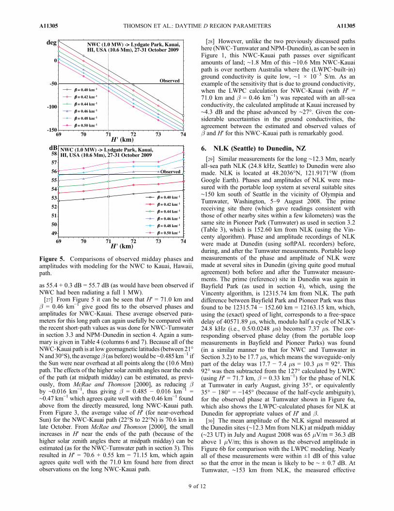
as 55.4 + 0.3 dB = 55.7 dB (as would have been observed ifNWC had been radiating a full 1 MW).[27] From Figure 5 it can be seen that H′ = 71.0 km and

b = 0.46 km−1 give good fits to the observed phases andamplitudes for NWC‐Kauai. These average observed para-meters for this long path can again usefully be compared withthe recent short‐path values as was done for NWC‐Tumwaterin section 3.3 and NPM‐Dunedin in section 4. Again a sum-mary is given in Table 4 (columns 6 and 7). Because all of theNWC‐Kauai path is at low geomagnetic latitudes (between 21°N and 30°S), the averageb (as before)would be∼0.485 km−1 ifthe Sun were near overhead at all points along the (10.6 Mm)path. The effects of the higher solar zenith angles near the endsof the path (at midpath midday) can be estimated, as previ-ously, from McRae and Thomson [2000], as reducing bby ∼0.016 km−1, thus giving b = 0.485 − 0.016 km−1 =∼0.47 km−1 which agrees quite well with the 0.46 km−1 foundabove from the directly measured, long NWC‐Kauai path.From Figure 3, the average value of H′ (for near‐overheadSun) for the NWC‐Kauai path (22°S to 22°N) is 70.6 km inlate October. From McRae and Thomson [2000], the smallincreases in H′ near the ends of the path (because of thehigher solar zenith angles there at midpath midday) can beestimated (as for the NWC‐Tumwater path in section 3). Thisresulted in H′ = 70.6 + 0.55 km = 71.15 km, which againagrees quite well with the 71.0 km found here from directobservations on the long NWC‐Kauai path.

[28] However, unlike the two previously discussed pathshere (NWC‐Tumwater and NPM‐Dunedin), as can be seen inFigure 1, this NWC‐Kauai path passes over significantamounts of land; ∼1.8 Mm of this ∼10.6 Mm NWC‐Kauaipath is over northern Australia where the (LWPC‐built‐in)ground conductivity is quite low, ∼1 × 10−3 S/m. As anexample of the sensitivity that is due to ground conductivity,when the LWPC calculation for NWC‐Kauai (with H′ =71.0 km and b = 0.46 km−1) was repeated with an all‐seaconductivity, the calculated amplitude at Kauai increased by∼4.3 dB and the phase advanced by ∼27°. Given the con-siderable uncertainties in the ground conductivities, theagreement between the estimated and observed values ofb and H′ for this NWC‐Kauai path is remarkably good.

6. NLK (Seattle) to Dunedin, NZ

[29] Similar measurements for the long ∼12.3 Mm, nearlyall‐sea path NLK (24.8 kHz, Seattle) to Dunedin were alsomade. NLK is located at 48.2036°N, 121.9171°W (fromGoogle Earth). Phases and amplitudes of NLK were mea-sured with the portable loop system at several suitable sites∼150 km south of Seattle in the vicinity of Olympia andTumwater, Washington, 5–9 August 2008. The primereceiving site there (which gave readings consistent withthose of other nearby sites within a few kilometers) was thesame site in Pioneer Park (Tumwater) as used in section 3.2(Table 3), which is 152.60 km from NLK (using the Vin-centy algorithm). Phase and amplitude recordings of NLKwere made at Dunedin (using softPAL recorders) before,during, and after the Tumwater measurements. Portable loopmeasurements of the phase and amplitude of NLK weremade at several sites in Dunedin (giving quite good mutualagreement) both before and after the Tumwater measure-ments. The prime (reference) site in Dunedin was again inBayfield Park (as used in section 4), which, using theVincenty algorithm, is 12315.74 km from NLK. The pathdifference between Bayfield Park and Pioneer Park was thusfound to be 12315.74 − 152.60 km = 12163.15 km, which,using the (exact) speed of light, corresponds to a free‐spacedelay of 40571.89 ms, which, modulo half a cycle of NLK’s24.8 kHz (i.e., 0.5/0.0248 ms) becomes 7.37 ms. The cor-responding observed phase delay (from the portable loopmeasurements in Bayfield and Pioneer Parks) was found(in a similar manner to that for NWC and Tumwater inSection 3.2) to be 17.7 ms, which means the waveguide‐onlypart of the delay was 17.7 − 7.4 ms = 10.3 ms ≡ 92°. This92° was then subtracted from the 127° calculated by LWPC(using H′ = 71.7 km, b = 0.33 km−1) for the phase of NLKat Tumwater in early August, giving 35°, or equivalently35° − 180° = −145° (because of the half‐cycle ambiguity),for the observed phase at Tumwater shown in Figure 6a,which also shows the LWPC‐calculated phases for NLK atDunedin for appropriate values of H′ and b.[30] The mean amplitude of the NLK signal measured at

the Dunedin sites (∼12.3 Mm from NLK) at midpath midday(∼23 UT) in July and August 2008 was 65 mV/m ≡ 36.3 dBabove 1 mV/m; this is shown as the observed amplitude inFigure 6b for comparison with the LWPC modeling. Nearlyall of these measurements were within ±1 dB of this valueso that the error in the mean is likely to be ∼ ± 0.7 dB. AtTumwater, ∼153 km from NLK, the measured effective

Figure 5. Comparisons of observed midday phases andamplitudes with modeling for the NWC to Kauai, Hawaii,path.

THOMSON ET AL.: DAYTIME D REGION PARAMETERS A11305A11305

9 of 12

midday mean amplitude of the NLK signal, 5–9 August2008, was 31.7 ± 2 mV/m ≡ 90.0 dB > 1 mV/m. UsingLWPC, with an appropriate (midday, early August, 47.5° N)ionosphere, H′ = 71.7 km, b = 0.33 km−1, on this NLK‐to‐Tumwater path, gave the radiated power as 290 kW. Thispower was then used again in LWPC to calculate theexpected amplitudes of NLK at Dunedin (12.3 Mm away)for appropriate values of H′ and b, giving the results shownin Figure 6b for comparison with the observed amplitude.[31] As for the other three long paths discussed here

(sections 3, 4, and 5), H′ and b for this long path can againusefully be estimated from the recently measured short‐path

parameters. Again a summary is given in Table 4 (columns8 and 9). From Figure 3, the average value of H′ (for near‐overhead Sun) for the NLK‐Dunedin path (48°N to 46°S,early August) is 70.0 km. FromMcRae and Thomson [2000],the increases in H′ near the ends of the path (because of thehigher solar zenith angles there at midpath midday) can beestimated (as for the NWC‐Tumwater path in section 3.3).This resulted in H′ = 70.0 + 0.8 km = 70.8 km. For the ∼60%of this NLK‐Dunedin path with low geomagnetic latitudesbetween 30°N and 30°S, the average b (as before) will be∼0.485 km−1, while for the remaining 40% of the path (theSeattle and Dunedin ends) the average b will be ∼(0.47 +0.34)/2 km−1 = 0.41 km−1, giving b = 0.6 × 0.485 + 0.4 ×0.41 km−1 = 0.455 km−1 for the Sun near the zenith all alongthe path. The effects on b of the actual higher solar zenithangles near the ends of the path (at midpath midday) can beestimated, as before, from McRae and Thomson [2000], asreducing b by ∼0.02 km−1, giving b = 0.455 − 0.02 km−1 =∼0.435 km−1, which does not agree very well with the∼0.38 km−1 indicated by the direct observations in Figure 6b.Indeed, as can be seen in Figure 6b, it appears that b =0.435 km−1 would give an observed amplitude at Dunedin of38.7 dB > 1mV/m whereas the actual portable loop observa-tions gave 36.3 dB at Dunedin.[32] This apparent discrepancy appears to be a result of

the effective radiated power from NLK being somewhatdirection dependent. NLK is unusual in that, instead ofusing very tall towers (400–500 m high) on flat ground tomake the antenna high enough to get a reasonable radiationefficiency, it has wires strung between mountain ridgesacross a valley with the radiating current coming up to thesein a cable from the transmitter on the valley floor below[e.g., Watt, 1967]. As well as the NLK amplitude mea-surements near Tumwater (∼153 km SSW of NLK), addi-tional amplitude measurements were made over a muchgreater land area and range of directions ∼SW of NLK (theclosest to NLK being at Dosewallips State Park, 93 km fromNLK, while the furthest was at Westport on the west coast,220 km from NLK). A range‐corrected plot of these mea-sured amplitudes of NLK as a function of azimuth (degreeseast of north from NLK) is shown in Figure 6c, where it canbe seen that the amplitudes measured at sites in the directionof Dunedin are ∼3 dB lower than those measured at sitesnear Tumwater. As the amplitudes at Tumwater were usedto determine the radiated power of 290 kW used for NLKin calculating the amplitudes at Dunedin in Figure 6b, itseems that the low amplitudes (∼36 dB) measured atDunedin may well be due to the lower radiated power in thisdirection. Thus quite likely the value of b = 0.435 km−1

estimated from the earlier short path measurements will bemore appropriate than the (radiation‐direction‐compro-mised) value, b = 0.38 km−1, from amplitude comparisonsin Figure 6b. Indeed, if b = 0.435 km−1 is used in the NLK‐Dunedin phase plot in Figure 6a, then this gives H′ =70.9 km, in close agreement with the H′ = 70.8 km esti-mated above from the short‐path parameters.

7. Discussion, Summary, and Conclusions

[33] Phases and amplitudes of suitable VLF signals weremeasured using a portable loop system referenced to GPS 1s pulses. Observations of the midday VLF radio phase

Figure 6. Comparisons of observed midday (a) phases and(b) amplitudes with modeling for the NLK to Dunedin pathplus (c) the observed directivity of NLK toward Dunedinand Tumwater.

THOMSON ET AL.: DAYTIME D REGION PARAMETERS A11305A11305

10 of 12

changes and amplitude attenuations along four long, mainlyall‐sea paths have been presented here: NWC (NW Aus-tralia) to Seattle, Washington (14.2 Mm), NPM (Hawaii) toDunedin, New Zealand (8.1 Mm), NWC to Kauai, Hawaii(10.6 Mm), and NLK (Seattle) to Dunedin, New Zealand(12.3 Mm). Average values of the height H′ and sharpness bof the D region of the ionosphere along each path were thendetermined by modeling with the waveguide code, LWPC,so that the modeled phases and amplitudes agreed withthose observed.[34] These resulting average values of H′ and b for each

of the four long paths were then compared with recent short‐path (∼300 km) measurements of H′ and b at (i) a lowgeomagnetic latitude and (ii) a middle‐high geomagneticlatitude. The interpolation of b with geomagnetic latitudealong the paths was obtained from these by using the knownvariation of cosmic ray flux with geomagnetic latitude. Thevariations (interpolations) of H′ with season and geographiclatitude along the paths were obtained from the short‐pathobservations by extending them with the MSIS‐E‐90 neutralatmosphere model. Small additional variations of H′ and bthat were due to changes in solar zenith angles near the endsof the paths were estimated from the observations of McRaeand Thomson [2000]. Han and Cummer [2010] measured H′near Duke University, ∼37°N geographic, in summer usingnatural lightning. Their values of H′ for near‐overhead Sunare typically in the range 71–72 km, averaging ∼71.5 km,which is a little greater than the H′ = 70.9 km from MSIS‐E‐90 and Figure 3 in June and July here, but is quite likely justwithin the combined experimental errors of the two methods.[35] For the NPM‐Dunedin path (8.1 Mm), both the direct

long‐path method and the interpolated‐extrapolated short‐path method gave essentially the same results, H′ = 70.8 kmand b = 0.46 km−1. The very long (14.2 Mm) NWC‐Seattlepath gave the same (average) value of b = 0.42 km−1 withboth short‐ and long‐path methods, while the H′ = 71.1 kmobtained from the long path was only marginally lower, by∼0.1 km (∼100 m), than the H′ = 71.2 km obtained using theshort‐path method. A similar small height difference wasalso seen on the (10.6 Mm) NWC‐Kauai path (H′ = 71.0 and71.15 km), but this is of even less significance because of theuncertainty in the (low) conductivity of the ∼1.8 Mm of(Australian) ground on this path. Similarly the differencebetween the short‐path and long‐path values of b for this path(0.47 and 0.46 km−1) is also probably not enough to be sig-nificant for the same uncertain ground conductivity reason.For the (12.3 Mm) NLK‐Dunedin path, in contrast with thetwo NWC paths, theH′ = 70.9 km from the long‐path methodwas slightly higher than the H′ = 70.8 km from the short‐path method. The uncertainties for b on this path, becauseof NLK and some of its nearby measurements being under-taken in mountainous terrain, mean that this small differencein H′ (0.1 km) is probably not significant for this path.[36] Overall, the agreement between the short‐path and

long‐path observations is remarkably good, with maximumdifferences of only ∼0.15 km in height H′ and 0.01 km−1 insharpness b. This is suggestive that the errors (∼ ± 0.5 kmfor H′ and ∼ ± 0.03 km−1 for b) for the short‐path mea-surements reported by Thomson [2010] and Thomson et al.[2011] may have been a little conservative. Because both thetransmitters and the measurement sites there were on landand the paths were short (∼300 km), there was a concern that

the resulting proportion of low‐conducting land and coastalboundaries (though appreciably less than for 50% of thepaths) might have been having more effect than hoped. Anyconcern that this might have been a difficulty is nowmarkedly reduced. The use of the MSIS model for esti-mating changes in H′ with season and latitude (but not withsolar zenith angle) effectively assumes there are no relevantneutral atmosphere composition changes (near 70 km alti-tude) with season and latitude. For the cosmic rays, whichionize all atmospheric constituents, this is very likely to bethe case. However, for the minor but important constituentNO (ionized by Lyman‐a) this is less certain. Nonetheless,the apparent agreement resulting from using MSIS with thisassumption may well be implying that the proportion of NOin the neutral atmosphere at heights near 70 km, at least forthe low latitudes and midlatitudes studied here, is fairlyconstant with season and latitude.[37] The validated, quiet time, daytime modeling presented

here provides an improved baseline for measuring a widevariety of perturbations to the lower D region and hence theEarth‐ionospherewaveguide. Such “perturbations” include thetransition from day to night (so improving nighttime para-meters [Thomson et al., 2007; Thomson and McRae, 2009]),the effects of solar flares [e.g., Thomson et al., 2005], and theeffects of particle precipitation [e.g., Rodger et al., 2007],which can perturb the day or night ionosphere.[38] Of course, although the modeling by LWPC seems

very good, it will not be perfect; better modeling will be foundin the future. In particular, the representation of the electrondensity versus height profile in the lowerD region by the twosimple parameters, H′ and b, though very good, is not likelyto be exact. However, the raw phase and amplitude mea-surements for the long paths measured here are independentof the current modeling; these measurements could well beused in future, improved modeling and thus determining(retrospectively) improved values for the height (and sharp-ness) of the lowest edge of the (D region of) the Earth’sionosphere. The sensitivity of these long paths to these Dregion parameters is quite high; the error of ±6° in phase and±0.7 dB in amplitude estimated for the 14.2 Mm NWC‐Tumwater path in section 3.2 corresponds (using Figure 2)to a sensitivity of less than approximately ±0.3 km in H′ and∼±0.01 km−1 in b. Also, as can be seen from Figure 2c,a (short‐term) change in height H′ (by, say, 1 km) while bremained constant, caused by (say) a simple vertical heightchange in the neutral atmosphere alone (i.e., where theheight of a fixed density, say 1021 m−3, changes by 1 km)will cause a phase change of ∼44°/km. In such a (constant‐b)case, the long‐term phase measurement sensitivity of ±6°corresponds to a height sensitivity of ∼ ± 0.15 km. For veryshort‐term changes over a few hours, sensitivities as low as±4° or ±0.1 km = ±100 m are likely for this very long path(if b is constant). Over much longer times, when b may notbe quite constant, and even without improved modeling,future long‐path measurements of H′ and b can potentiallymeasure changes in height (of ∼0.3 km) over time to a higheraccuracy than current modeling can determine absoluteheight. Clearly such potential observations could includedetermining H′ changes over a solar cycle. It might also bepossible to use such height changes (averaged over individualsolar cycles), over even longer periods of time, to test theoriesof global warming and the corresponding height‐integrated

THOMSON ET AL.: DAYTIME D REGION PARAMETERS A11305A11305

11 of 12

atmospheric expansions and contractions below a specifiedheight in the D region, such as H′, which correspondseffectively to the (fixed) density level down to which theexternal ionizing radiations (Lyman‐a, galactic cosmic rays,etc.) penetrate before they are absorbed or their effects areoverwhelmed by electron loss processes (attachment orrecombination).

[39] Acknowledgments. The authors are very grateful to their col-league, David Hardisty, for his design, development, and construction ofthe VLF phase meter. Thanks also to http://rimmer/ngdc.noaa.gov ofNGDC, NOAA, U.S. Dept. of Commerce, for the digital coastal outlineused in Figure 1.[40] Robert Lysak thanks the reviewers for their assistance in evaluat-

ing this manuscript.

ReferencesClilverd, M. A., et al. (2009), Remote sensing space weather events:Antarctic‐Arctic Radiation‐belt (Dynamic) Deposition‐VLF AtmosphericResearch Konsortium network, Space Weather, 7, S04001, doi:10.1029/2008SW000412.

Dowden, R. L., and C. D. D. Adams (2008), SoftPAL, paper presented atthe Third VERSIMWorkshop, Eötvös Univ., Tihany, Hungary, 15–20 Sept.

Ferguson, J. A., and F. P. Snyder (1990), Computer programs for assessmentof long wavelength radio communications, version 1.0: Full FORTRANcode user’s guide, Nav. Ocean Syst. Cent. Tech. Doc. 1773, DTIC AD‐B144839, Def. Tech. Inf. Cent., Alexandria, Va.

Han, F., and S. A. Cummer (2010), Midlatitude daytime D region iono-sphere variations measured from radio atmospherics, J. Geophys. Res.,115, A10314, doi:10.1029/2010JA015715.

McRae, W. M., and N. R. Thomson (2000), VLF phase and amplitude:Daytime ionospheric parameters, J. Atmos. Sol. Terr. Phys., 62(7),609–618, doi:10.1016/S1364-6826(00)00027-4.

McRae, W. M., and N. R. Thomson (2004), Solar flare induced ionosphericD‐region enhancements from VLF phase and amplitude observations,J. Atmos. Sol. Terr. Phys., 66(1), 77–87, doi:10.1016/j.jastp.2003.09.009.

Morfitt, D. G., and C. H. Shellman (1976), MODESRCH, an improvedcomputer program for obtaining ELF/VLF/LF mode constants in anEarth‐ionosphere waveguide, Nav. Electr. Lab. Cent, Interim Rep. 77T,NTIS Accession ADA032573, Natl. Tech. Inf. Serv., Springfield, Va.

Rodger, C. J., M. A. Clilverd, N. R. Thomson, R. J. Gamble, A. Seppälä,E. Turunen, N. P. Meredith, M. Parrot, J.‐A. Sauvaud, and J.‐J. Berthelier(2007), Radiation belt electron precipitation into the atmosphere: Recoveryfrom a geomagnetic storm, J. Geophys. Res., 112, A11307, doi:10.1029/2007JA012383.

Thomson, N. R. (1993), Experimental daytime VLF ionospheric parameters,J. Atmos. Terr. Phys., 55, 173–184, doi:10.1016/0021-9169(93)90122-F.

Thomson, N. R. (2010), Daytime tropical D region parameters from shortpath VLF phase and amplitude, J. Geophys. Res., 115, A09313, doi:10.1029/2010JA015355.

Thomson, N. R., and W. M. McRae (2009), Nighttime ionosphericD region: Equatorial and nonequatorial, J. Geophys. Res., 114, A08305,doi:10.1029/2008JA014001.

Thomson, N. R., C. J. Rodger, and M. A. Clilverd (2005), Large solar flaresand their ionospheric D region enhancements, J. Geophys. Res., 110,A06306, doi:10.1029/2005JA011008.

Thomson, N. R., M. A. Clilverd, and W. M. McRae (2007), Nighttime iono-spheric D region parameters from VLF phase and amplitude, J. Geophys.Res., 112, A07304, doi:10.1029/2007JA012271.

Thomson, N. R.,M.A. Clilverd, andC. J. Rodger (2011), DaytimemidlatitudeD region parameters at solar minimum from short‐path VLF phase andamplitude, J. Geophys. Res., 116, A03310, doi:10.1029/2010JA016248.

Vincenty, T. (1975), Direct and inverse solutions of geodesics on the ellip-soid with application of nested equations, Surv. Rev., 22(176), 88–93.

Wait, J. R., and K. P. Spies (1964), Characteristics of the Earth‐ionospherewaveguide for VLF radio waves, NBS Tech. Note 300, Natl. Bur. ofStand., Boulder, Colo.

Watt, A. D. (1967), VLF Radio Engineering, Elsevier, New York.

M. A. Clilverd, Physical Sciences Division, British Antarctic Survey,High Cross, Madingley Road, Cambridge CB3 0ET, UK.C. J. Rodger and N. R. Thomson, Physics Department, University of

Otago, PO Box 56, Dunedin 9016, New Zealand. (n_thomson@physics.otago.ac.nz)

THOMSON ET AL.: DAYTIME D REGION PARAMETERS A11305A11305

12 of 12