Embed Size (px)
Citation preview
Day Trading Profitability across Volatility States: Evidence of
Intraday Momentum and Mean Reversion
Christian Lundström
Department of Economics
Umeå School of Business and Economics
Umeå University
SE-901 87 Umeå
Abstract
Recent research links the profitability of a popular day trading strategy, the Opening Range
Breakout (ORB), to intraday momentum. In this paper we link the ORB profitability to
intraday volatility of the underlying asset and thereby propose intraday volatility as a factor
generating time-varying market inefficiencies creating profit opportunities for day traders.
When applied to long time series of futures prices we find significant differences in ORB
returns across volatility states indicating momentum (mean reversion) in periods of high
(low) volatility, and with efficient prices in-between.
Key words: Opening Range Breakout strategies, Time-varying market inefficiency, Crude oil futures,
S&P 500 futures, Technical trading, Contraction-Expansion principle.
JEL classification: C49, G11, G14, G17.
We thank Kurt Brännäs, Tomas Sjögren, Thomas Aronsson, Rickard Olsson and Erik Geijer for insightful comments and suggestions.
1
1. Introduction
Day traders are relatively few in persons but accounts for a relatively large part of the traded
volume in the market place (e.g., Barber and Odean, 1999; Barber et al., 2011; Kuo and Lin,
2013). Day trading profitability is considered a lottery and long-run profitability is therefore
something of a mystery (Statman, 2002). The profitability of day traders is related to the
research by Harris and Schultz (1998), Jordan and Diltz (2003), Garvey and Murphy (2005),
Linnainmaa (2005), Coval et al. (2005), Barber et al. (2006, 2011) and Kuo and Lin (2013),
who study trading accounts for various stock- and futures exchanges. When measuring day
trading profitability using transactions from individual accounts, the trades initiated and
executed in the same trading day are used to calculate the average returns. Most studies
find that there is empirical evidence of only a relatively small fraction of day traders being
profitable. Approximately one in five day traders are able to achieve significant profitability
after transaction costs (e.g., Coval et al., 2005; Barber et al., 2011; Kuo and Lin, 2013).
Linnainmaa (2005) finds no evidence of profitability from day trading.
The existence of some individual day traders achieving long-run profitability goes against the
supposedly random outcome of a lottery (e.g., Statman, 2002) but none of these studies
addresses which possible trading strategy, or strategies, that may have been used to obtain
this significant profitability. Holmberg, Lönnbark and Lundström (2013), hereafter HLL, link
the profitability of a popular day trading strategy, the Opening Range Breakout (ORB)
strategy, to so-called intraday momentum in asset prices. When applied to a long time series
of crude oil futures they find significant ORB profitability for a hypothetical trader but when
splitting the data series into smaller time periods, however, they find profitability only in the
last time period ranging from 2001-10-12 to 2011-01-26. The seemingly time-dependence of
day trading profitability is the motivation behind this study.
In this paper we link the ORB profitability to intraday volatility of the underlying asset. Due
to this intimate relation we expect that the profitability of ORB traders should coincide over
time with volatility clustering (e.g. Engle, 1982). This would explain the significant ORB
profitability in the period 2001-10-12 to 2011-01-26, found in HLL, as it contain the extreme
volatility associated with the sub-prime market turmoil. From this insight we find it fruitful to
test the profitability across volatility states. To assess the daily returns of the ORB strategy
2
we follow the basic outline as in HLL but with a slight improvement providing a closer
approximation to the ORB returns as originally suggested in Crabel (1990). When applied to
long time series of crude oil futures and to S&P 500 index futures, respectively, we find
significant changes in ORB profitability levels across volatility states. The profitability
differences between the lowest volatility state and the highest volatility state are remarkably
high, around 200 basis points per day for crude oil and around 150 basis points per day for
S&P 500.
This undertaking relates to recent literature regarding the possibility that market efficiency
may vary over time generated by some economic factor (see Lim and Brooks, 2011 for a
survey of the literature on time-varying market inefficiency). In particular, Lo (2004) and Self
and Mathur (2006) emphasize that since trader rationality as well as institutions evolve over
time, financial markets may experience long periods of market inefficiency followed by a
long period of market efficiency and vice versa. The possible existence of time-varying
market inefficiency is of course of interest for the fundamental understanding of financial
markets and the behavior of asset prices.
The main contribution of this paper is that we propose intraday volatility as a factor
generating time-varying market inefficiencies creating intraday profit opportunities for day
traders. As ORB profitability is linked to intraday momentum (e.g. HLL) as well, we are able
to relate momentum to periods of high intraday volatility, and reverse intraday momentum
or mean reversion, to periods of low intraday volatility, and with efficient prices in-between.
Both intraday momentum and mean reversion are anomalies of the efficient market
hypothesis (EMH) of Fama (1965, 1970) and has to the best of this author’s knowledge not
previously been linked to intraday volatility, theoretically or empirically. Moreover, as
volatility increases during time periods of market turmoil due to large price movements we
may from our findings add the ORB strategy to the class of trading strategies that generate
so-called “crisis alpha” (e.g., Kaminski, 2011). Further, our results highlight the need for
relatively long time series when evaluating day trading profitability containing a wide range
of volatility realizations to avoid possible volatility bias. Harris and Schultz (1998), for
example, study day trading profitability over only a three-week period, and Garvey and
Murphy (2005) over a three-month period. As volatility clusters in financial returns series are
somewhat predictable (e.g., Engle, 1982) our results suggests adding volatility predictors to
3
day trading to increase expected profitability (models to predict the volatility of the S&P 500
can be found in Martens et al. 2009).
Studies of day trading profitability in futures markets, rather than in stock markets, are to
the best of our knowledge only to be found in the very recent work by HLL and Kuo and Lin
(2013), and have some advantages. First, costs associated with trading such as commissions
and bid ask spreads are often considerably smaller in futures contracts than in stocks due to
the relatively high liquidity in some futures contracts, and second, futures are as easily sold
short as bought long and are not subject to short-selling restrictions. Crude oil and S&P 500
offers the most liquid future contracts available and probably the least affected by trading
costs. These futures contracts are also tested in Crabel (1990) and Williams (1999).
Day traders may trade according to other strategies than the ORB strategy (e.g., Marshall et
al., 2008; Yamamoto, 2012, and see also Schulmeister, 2009), and the profitability of day
trading strategies may coincide with other factors besides volatility but the ORB strategy,
and intraday volatility, is the only strategy and factor considered in this paper.
The remainder of the paper is organized as follows. In Section 2 we illustrate the relation
between ORB profitability and momentum. In this Section we also illustrate the relation
between ORB profitability and intraday volatility. In Section 3 we outline the profitability
tests. Section 4 describes the data and we give the results of the empirical tests. In Section 5
we discuss the results.
4
2. The ORB Strategy
The ORB strategy is based on the premise that if the price moves a certain percentage from
the opening price level, the odds favor a continuation of that move until the closing price of
that day. The ORB strategy suggests that long (short) positions are established at some
predetermined price threshold a certain percentage above (below) the opening price,
respectively (Crabel, 1990). Profitability of the ORB strategy imply that the asset price must
follow so-called intraday momentum at the price threshold levels, i.e., the tendency for
rising asset prices to rise further and falling prices to keep falling, HLL. In this sense, intraday
momentum can be related to momentum found in monthly returns data (Jegadeesh and
Titman, 1993; Miffre and Rallis, 2007).
The so-called Contraction-Expansion (C-E) principle provides a possible rationale behind ORB
profitability, Crabel (1990). The principle is based on the observation that daily price
movements seem to alternate between regimes of contraction and expansion, or, periods of
modest and large price movements, respectively. In particular, the prices are characterized
by intraday momentum during expansion days, whereas during contraction days, prices
move randomly, Crabel (1990). We note a resemblance between the C-E principle and of
volatility clustering in financial returns series (e.g. Engle, 1982). As most days are contraction
days (Crabel, 1990) an ORB strategy may be viewed as a strategy of identifying and profiting
from days of price expansion and avoiding contraction days.
In the behavioral finance literature the appearance of momentum is often attributed to
cognitive biases from irrational investors such as investor herding, investor over- and under
reaction, and confirmation bias (e.g. Barberis et al., 1998; Daniel et. al., 1998). However, as
discussed in Crombez (2001) momentum can also be observed with perfectly rational traders
if we assume noise in the experts’ information. The reason why momentum may appear is,
however, outside the scope of this paper.
We now illustrate the ORB strategy in theory and we provide a link between ORB returns
and intraday momentum in prices. We follow the basic outline of HLL but for convenience
we model the natural logarithm of prices. We denote by and
the opening and closing
log prices of day , respectively. We assume that prices are traded continuous within a
trading day where a point on day t is given by , . Note that and
5
. Further, we let
and denote threshold price levels such that if the price
crosses it from below (above) the ORB trader initiates a long (short) position. These
threshold prices are placed at some predetermined distance from the opening price, ,
i.e. and
. We use symmetrically placed thresholds for long and
short positions, assuming that day traders has no ex ante bias regarding possible trend
direction.
Within the context of this paper it is natural to involve the martingale pricing model (MPT) of
Samuelson (1965); If capital markets are efficient with respect to the information set
all linear forecasting rules for future price changes based on alone should not result in
any systematic success. In particular, we may write the martingale property of prices, and
returns, respectively, as follows;
[ | ]
[ | ] [ | ]
Relating the ORB profitability to the , we test here if the martingale property holds at
the proposed price thresholds, i.e. when initiating a long (short) position at the threshold
( ) and hold until market close, ;
[ | ]
[ | ]
where represents the first point in time, during the trading day, when a
threshold is crossed. This inequalities test is equally a test of intraday momentum with
equality under the MPT.
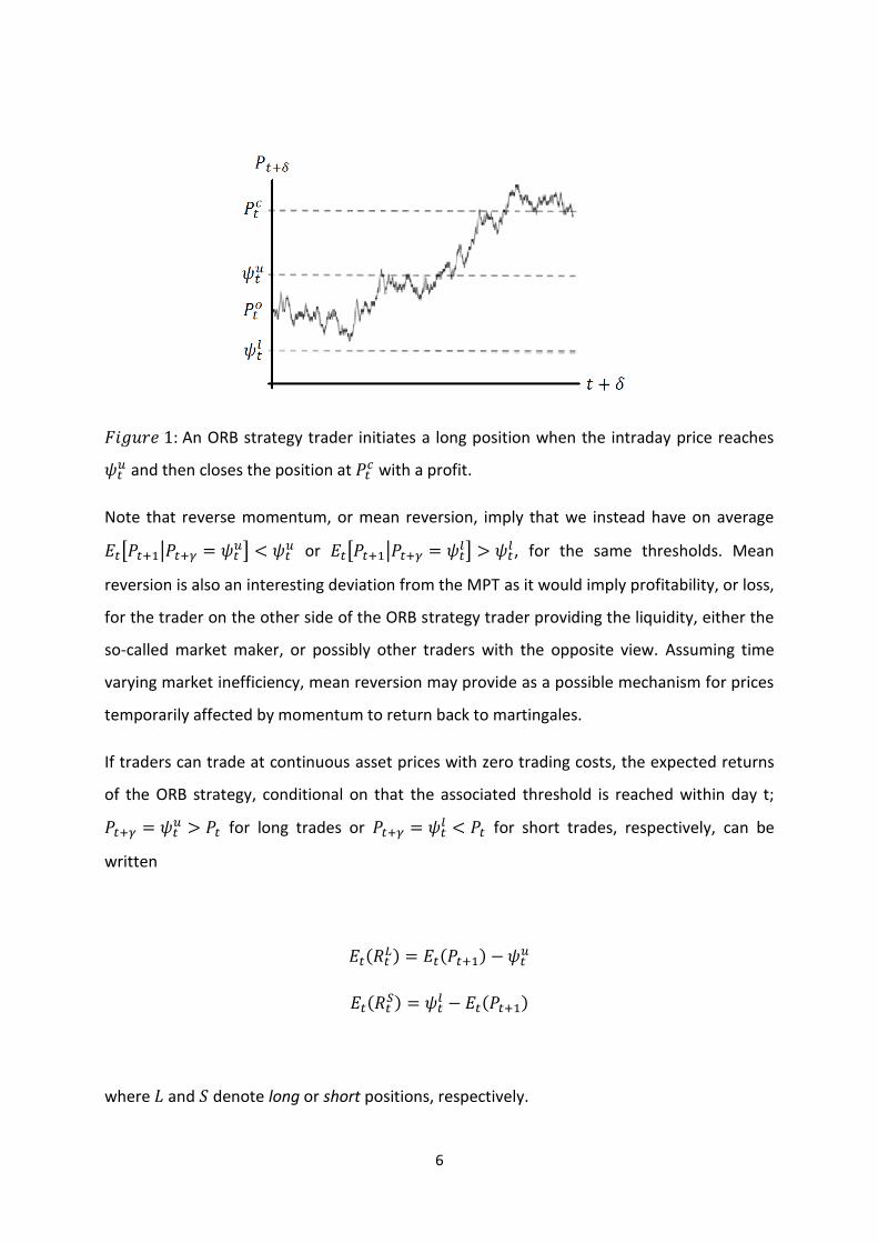
We illustrate how a winning ORB position may evolve during the course of a trading day, in
.
6
: An ORB strategy trader initiates a long position when the intraday price reaches
and then closes the position at
with a profit.
Note that reverse momentum, or mean reversion, imply that we instead have on average
[ | ]
or [ | ]
, for the same thresholds. Mean
reversion is also an interesting deviation from the MPT as it would imply profitability, or loss,
for the trader on the other side of the ORB strategy trader providing the liquidity, either the
so-called market maker, or possibly other traders with the opposite view. Assuming time
varying market inefficiency, mean reversion may provide as a possible mechanism for prices
temporarily affected by momentum to return back to martingales.
If traders can trade at continuous asset prices with zero trading costs, the expected returns
of the ORB strategy, conditional on that the associated threshold is reached within day t;
for long trades or
for short trades, respectively, can be
written
( ) ( )
( )
( )
where and denote long or short positions, respectively.
7
If prices are martingales we have from MPT; ( ) and (
) . If prices are
instead driven by momentum we have; ( ) and (
) , or by mean-reversion;
( ) and (
) .
We now link the ORB profitability to intraday volatility of the underlying asset.
Note that even if futures contracts may trade for 24 hours the ORB strategy is based on the
US market opening hours, Crabel (1990). This is also the time when the liquidity is the
highest. For all other time periods we assume that the trader is out of the market, in cash.
Hence for the ORB trader, only intraday volatility during the US market opening hours is of
interest.
Andersen and Bollerslev (1998) argue that in most financial applications the asset price is
assumed to follow a continuous time diffusion process, and hence the correct measure for
intraday volatility is
∫
where the diffusion process, for this application, is defined over the intraday time interval of
the US market opening hours. If we assume that the instantaneous returns are generated by
the continuous time martingale such as , where denotes a standard
Wiener process, it follows from Ito´s Lemma, Andersen and Bollerslev (1998);
∫ (
)
(∫
) (∫( )
) ( )
where ( )
is squared open-to-close returns.
8
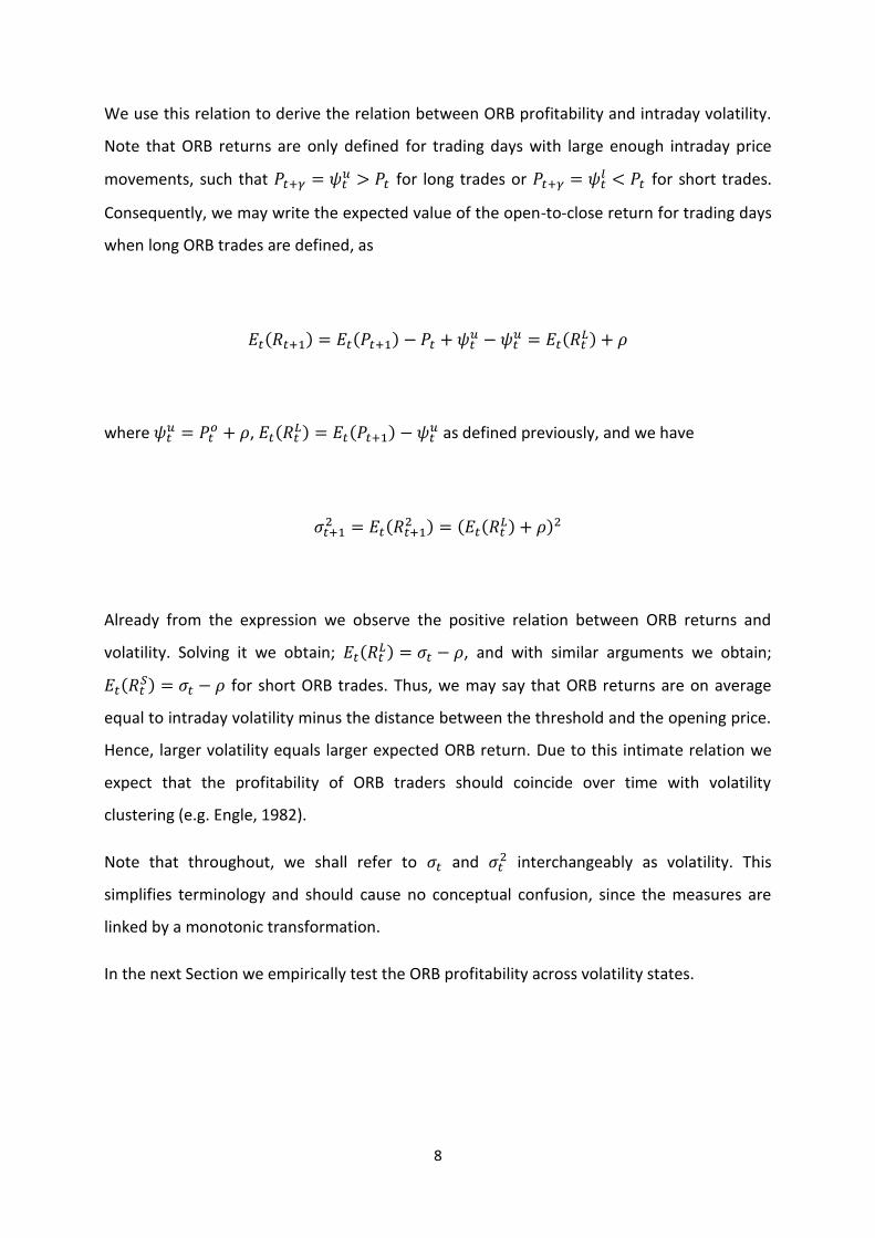
We use this relation to derive the relation between ORB profitability and intraday volatility.
Note that ORB returns are only defined for trading days with large enough intraday price
movements, such that for long trades or
for short trades.
Consequently, we may write the expected value of the open-to-close return for trading days
when long ORB trades are defined, as
( ) ( )
( )
where
, ( ) ( )
as defined previously, and we have
(
) ( ( ) )
Already from the expression we observe the positive relation between ORB returns and
volatility. Solving it we obtain; ( ) , and with similar arguments we obtain;
( ) for short ORB trades. Thus, we may say that ORB returns are on average
equal to intraday volatility minus the distance between the threshold and the opening price.
Hence, larger volatility equals larger expected ORB return. Due to this intimate relation we
expect that the profitability of ORB traders should coincide over time with volatility
clustering (e.g. Engle, 1982).
Note that throughout, we shall refer to and interchangeably as volatility. This
simplifies terminology and should cause no conceptual confusion, since the measures are
linked by a monotonic transformation.
In the next Section we empirically test the ORB profitability across volatility states.
9
3. Profitability Tests
We now assess the hypothetical profitability of a day trader applying the ORB day trading
strategy to crude oil futures and to S&P 500 futures. Assessing the hypothetical profitability
of traders by applying technical trading rules on empirical asset prices is nothing new; see
Park and Irwin (2007) for an overview. In particular, the testing of technical trading rules
applied on commodity futures for longer investment horizon than intraday can be found in
Miffre and Rallis (2007) and Marshall et al. (2008).
Knowing that ORB profitability is related to volatility we recognize some advantages using
technical trading strategies relative to studying individual trading accounts as in previous
studies. First, we may test longer time series which is valuable in order to avoid possible
volatility bias, and second, we know that trading strategies are solely used to generate
profits. When studying trading accounts trades could also have been made for other reasons
than for profitability; consumption, liquidity, portfolio rebalancing, diversification, hedging
or tax motives, to mention a few, creating potentially noisy estimates. The major
disadvantages when testing profitability using technical trading strategies arises if the
strategies are developed by researchers. If we want to assess the returns of traders, the
proposed strategy must be known to, as well as used by, traders at the time of their trading
decisions, see the discussion in Coval et al. (2005). Further, even if the strategy has been
used among traders, the researcher could potentially over-fit the strategy parameters to the
historical data and in effect over-estimate the actual profitability, i.e., the problem with data
snooping (e.g., Sullivan et al. 1999; White, 2000). As the ORB strategy was both recognized
and exploited by traders (e.g., Williams, 1999) and we test the profitability using data from
1991 until today, subsequent to the publication of the ORB strategy in Crabel (1990), we
avoid the problem pointed out in Coval et al. (2005). As the ORB strategy is defined by only
one parameter, the predetermined distance to determine the threshold price levels, we test
the profitability for a large number of possible parameter values. Thereby we avoid the
problem of data snooping.
In order to empirically test for day trading profitability we first need to assess the realized
intraday ORB returns. Although limited to price series with readings only of the daily
opening, high, low, and closing prices, we are able to assess the intraday ORB returns
10
following the approach of HLL. We denote by ,
, and
the open, high, low and,
close reading of the natural logarithm of prices on day . Relating these empirical measures
to those of our theoretical illustration we interpret ,
,
and . The basic observation is that if the daily high;
, is higher than the
, or if the daily low;
, is lower than , we know with certainty that a buy or sell signal
was triggered during the trading day (HLL). This approach allows us to study day trading
profitability over long time periods. For now we assume that traders can trade at continuous
asset prices within a trading day at zero trading costs. We discuss the effects of possible
discontinuous jumps in prices, and of positive trading costs, on our results in the empirical
results.
From HLL the strategy returns for long trades; , and short trades,
, can be written,
respectively;
This is also a straightforward returns assessment given the theoretical illustration. As can be
seen;
, only profits from positive price trends, and;
, only profits
from negative price trends, respectively. The HLL approach may under-estimate the ORB
profitability of Crabel (1990) as day traders should be able to profit from long as well as
short positions, whichever comes first. Further, to increase the average profitability of the
strategy the ORB trader is supposed to limit intraday losses, using a so-called stop loss order
placed a distance below (above) a long (short) position, respectively (Crabel, 1990). Using
the HLL approach, however, both and
carry unlimited intraday risk.
We present a new approach to overcome these shortcomings when assessing the ORB
returns while still being applicable to daily time series. We denote it the “ORB Long Strangle”
strategy as it is a futures trader’s equivalent to a Long Strangle option strategy (e.g., Saliba et
al., 2009) applied intraday. The ORB Long Strangle is done in practice by placing two resting
11
market orders; a long position at but also a short position at
, both positions remaining
active throughout the trading day. Consequently, the strategy produces one out of three
possible outcomes; 1) Only the upper threshold is crossed yielding the return equal to . 2)
Only the lower threshold is crossed yielding the return equal to . 3) Both thresholds are
crossed, i.e., double crossing, yielding the return equal to (
) . Note that if the
trader experiences a double crossing, the remainder of the day is left alone from trading in
line with Crabel (1990). This is satisfied in the Long Strangle strategy as there are only two
active orders during one day which rule out triple crossings. The returns of the Long Strangle
strategy, , can hence be written;
{
(
) (
) (
)
(
) (
) (
)
(
) (
) (
)
From the returns calculations we find that the ORB Long Strangle profits from both positive
and negative price trends, whichever comes first, and in effect uses the opposite threshold
as a stop limiting intraday losses to (
) . The ORB Long Strangle returns hence
provide a closer approximation to the returns of Crabel (1990) and provide a more realistic
estimate of actual day trading profitability compared to the approach of HLL.
To empirically test ORB profitability we estimate the constant term of the following
specification given some level of :
where
∑ [(
) (
)]
∑ [(
) (
)]
12
is the average ORB return, the error term, and [ ] is the indicator function.
For ORB profitability given threshold we expect , which hence also indicates
intraday momentum. For intraday mean reversion we expect; , and under the
null hypothesis of prices being martingales.
As ORB returns are not defined every day, but only at expansion days, the potential
autocorrelation structure we may find in the open-to-close returns, ( ), is naturally broken
when we perform the ORB return transformation and we expect no serial correlation in
. From the strong relation between ORB returns and intraday volatility, however, we
recognize that ORB returns should experience heteroscedasticity and we use a Generalized
Least Squares estimation with HAC corrected standard errors (e.g., MacKinnon and White,
1985) to assess statistical significance.
For the purpose of this paper we also attempt to study day trading profitability across
volatility states. We first group the returns into volatility states based on deciles of the
intraday volatility distribution ranked from low to high, with the decile as the state
with the highest volatility, and the decile as the state of lowest volatility, respectively.
We then calculate the average ORB return associated to each state.
In order to empirically test the ORB profitability across volatility states we consider the
following dummy variable specification, given some level of :
∑
where | is the average ORB return in the volatility state, is a binary
variable, and is the error term. if the returns corresponds to the decile of
the intraday volatility distribution, zero otherwise.
From this specification we obtain information of the ORB profitability changes across the
entire range of 10 intraday volatility states. As ORB returns are positively related to intraday
13
volatility we expect that; for . Note that since each state roughly contains
only one of the full sample of observations we denote the state-specific average
return, , as short-run profitability and the average return using the full sample, , as the
long-run profitability. In addition, testing the short-run together with the long-run average
return allow us to study to what extent long-run losing traders ( ) may experience
short-run positive profitability on average ( ) during high volatility states, as well as
to what extent long-run profitable traders ( ) may experience short-run negative
profitability on average ( ) during low volatility states.
This test requires that we estimate intraday volatility. Unfortunately, however, volatility is
not directly observable. Assuming that ∫
is the correct measure for intraday
volatility we need a suitable estimator. Limited to daily price series we use the open-to-close
absolute return of day to estimate intraday volatility;
| | |
|
which is an unbiased estimator of intraday volatility as ( )
| | .
Although | | is an unbiased, it is noisy, Andersen and Bollerslev (1998). One extreme
example would be a very volatile day with widely fluctuating prices, but where the closing
price is the same as the opening price. The daily open-to-close absolute return would then
equal zero, whereas the actual volatility has been non-zero. As ORB profitability implies a
closing price at a relatively large distance from the opening prince, we expect reduction in
noise when measuring ORB profitability in the higher volatility states.
In the next section we present the data and the empirical results.
14
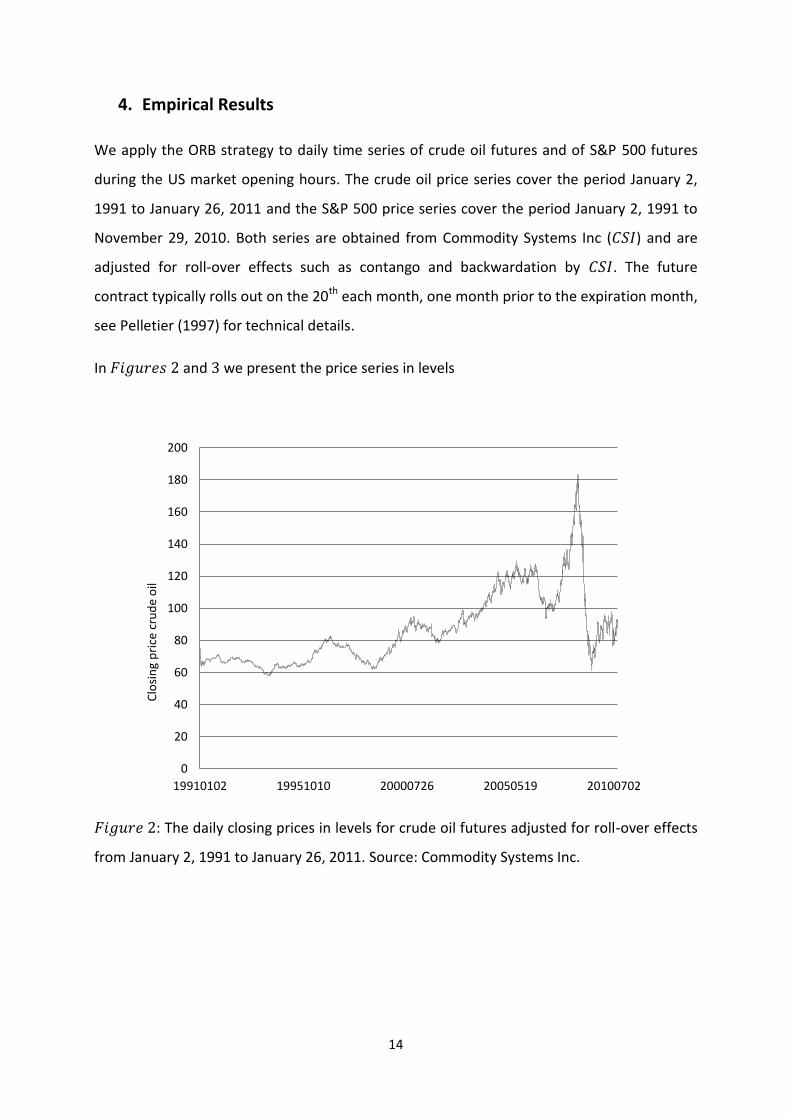
4. Empirical Results
We apply the ORB strategy to daily time series of crude oil futures and of S&P 500 futures
during the US market opening hours. The crude oil price series cover the period January 2,
1991 to January 26, 2011 and the S&P 500 price series cover the period January 2, 1991 to
November 29, 2010. Both series are obtained from Commodity Systems Inc ( ) and are
adjusted for roll-over effects such as contango and backwardation by . The future
contract typically rolls out on the 20th each month, one month prior to the expiration month,
see Pelletier (1997) for technical details.
In and we present the price series in levels
: The daily closing prices in levels for crude oil futures adjusted for roll-over effects
from January 2, 1991 to January 26, 2011. Source: Commodity Systems Inc.
0
20
40
60
80
100
120
140
160
180
200
19910102 19951010 20000726 20050519 20100702
Clo
sin
g p
rice
cru
de
oil
15
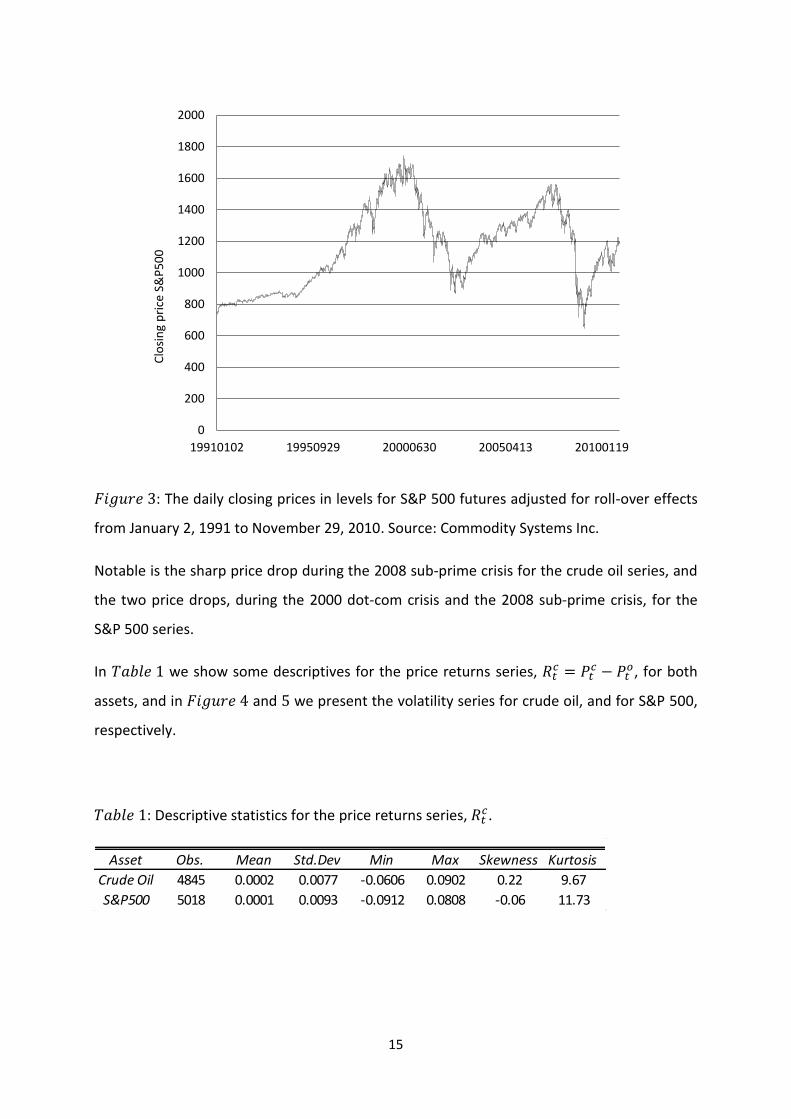
: The daily closing prices in levels for S&P 500 futures adjusted for roll-over effects
from January 2, 1991 to November 29, 2010. Source: Commodity Systems Inc.
Notable is the sharp price drop during the 2008 sub-prime crisis for the crude oil series, and
the two price drops, during the 2000 dot-com crisis and the 2008 sub-prime crisis, for the
S&P 500 series.
In we show some descriptives for the price returns series,
, for both
assets, and in and we present the volatility series for crude oil, and for S&P 500,
respectively.
: Descriptive statistics for the price returns series, .
0
200
400
600
800
1000
1200
1400
1600
1800
2000
19910102 19950929 20000630 20050413 20100119
Clo
sin
g p
rice
S&
P5
00
Asset Obs. Mean Std.Dev Min Max Skewness Kurtosis
Crude Oil 4845 0.0002 0.0077 -0.0606 0.0902 0.22 9.67
S&P500 5018 0.0001 0.0093 -0.0912 0.0808 -0.06 11.73
16
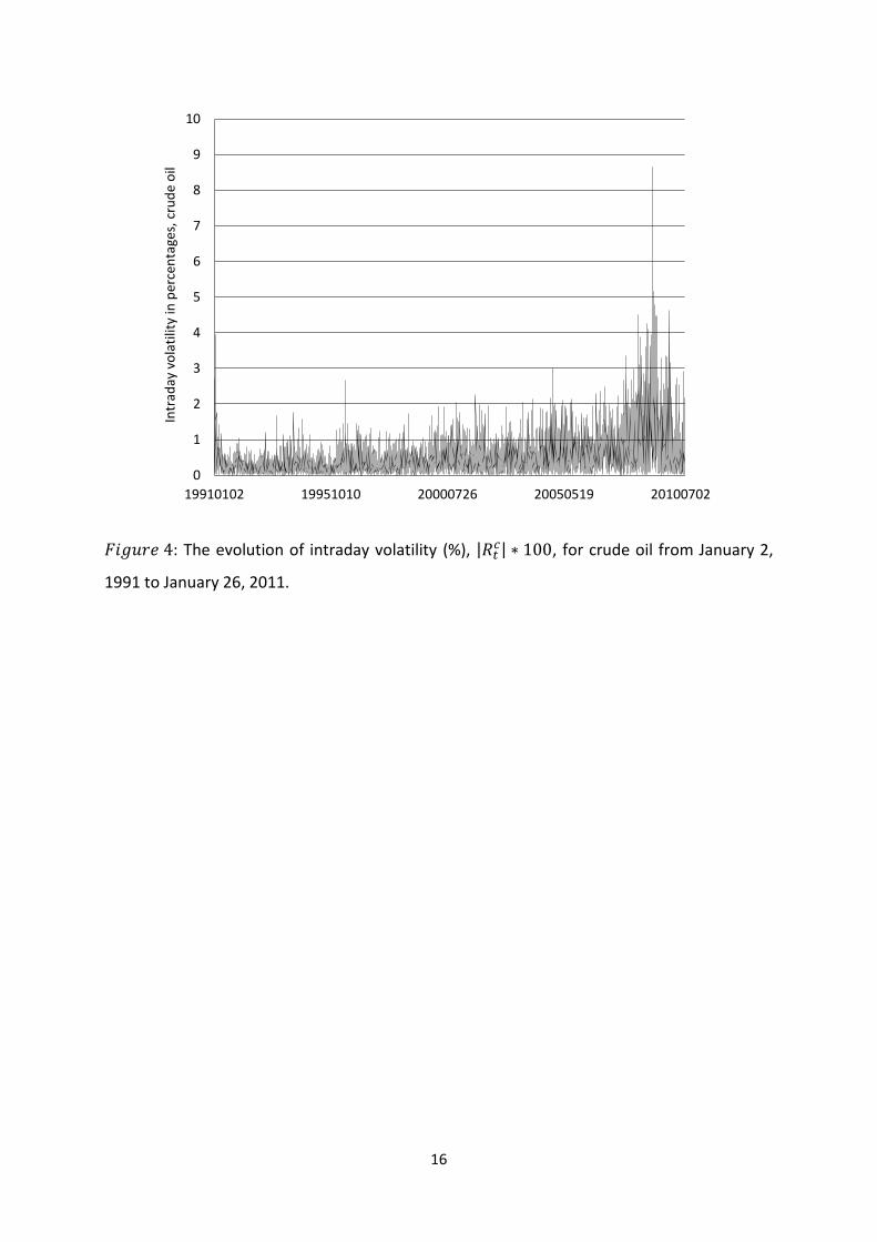
: The evolution of intraday volatility (%), | | , for crude oil from January 2,
1991 to January 26, 2011.
0
1
2
3
4
5
6
7
8
9
10
19910102 19951010 20000726 20050519 20100702
Intr
aday
vo
lati
lity
in p
erce
nta
ges,
cru
de
oil
17
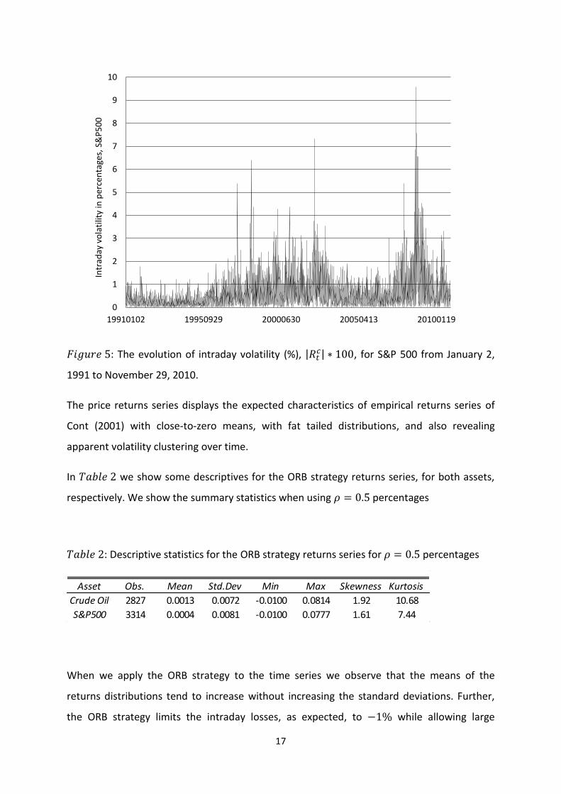
: The evolution of intraday volatility (%), | | , for S&P 500 from January 2,
1991 to November 29, 2010.
The price returns series displays the expected characteristics of empirical returns series of
Cont (2001) with close-to-zero means, with fat tailed distributions, and also revealing
apparent volatility clustering over time.
In we show some descriptives for the ORB strategy returns series, for both assets,
respectively. We show the summary statistics when using percentages
: Descriptive statistics for the ORB strategy returns series for percentages
When we apply the ORB strategy to the time series we observe that the means of the
returns distributions tend to increase without increasing the standard deviations. Further,
the ORB strategy limits the intraday losses, as expected, to while allowing large
0
1
2
3
4
5
6
7
8
9
10
19910102 19950929 20000630 20050413 20100119
Intr
aday
vo
lati
lity
in p
erce
nta
ges,
S&
P5
00
Asset Obs. Mean Std.Dev Min Max Skewness Kurtosis
Crude Oil 2827 0.0013 0.0072 -0.0100 0.0814 1.92 10.68
S&P500 3314 0.0004 0.0081 -0.0100 0.0777 1.61 7.44
18
positive returns increasing the skewness of the distributions. We now turn to the
profitability tests previously outlined.
We test the ORB profitability for a large number of thresholds. For simplicity, and without
loss of information, we present the results of only the following thresholds expressed in
percentages; { } used for both assets, respectively.
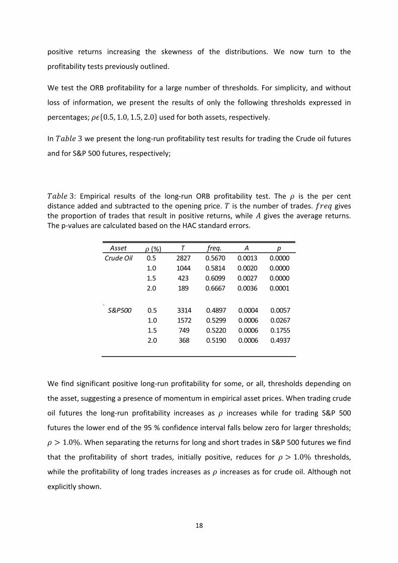
In we present the long-run profitability test results for trading the Crude oil futures
and for S&P 500 futures, respectively;
: Empirical results of the long-run ORB profitability test. The is the per cent distance added and subtracted to the opening price. is the number of trades. gives the proportion of trades that result in positive returns, while gives the average returns. The p-values are calculated based on the HAC standard errors.
We find significant positive long-run profitability for some, or all, thresholds depending on
the asset, suggesting a presence of momentum in empirical asset prices. When trading crude
oil futures the long-run profitability increases as increases while for trading S&P 500
futures the lower end of the 95 % confidence interval falls below zero for larger thresholds;
. When separating the returns for long and short trades in S&P 500 futures we find
that the profitability of short trades, initially positive, reduces for thresholds,
while the profitability of long trades increases as increases as for crude oil. Although not
explicitly shown.
Asset T freq. A p
Crude Oil 0.5 2827 0.5670 0.0013 0.0000
1.0 1044 0.5814 0.0020 0.0000
1.5 423 0.6099 0.0027 0.0000
2.0 189 0.6667 0.0036 0.0001
(%)
S&P500 0.5 3314 0.4897 0.0004 0.0057
1.0 1572 0.5299 0.0006 0.0267
1.5 749 0.5220 0.0006 0.1755
2.0 368 0.5190 0.0006 0.4937
(%)
19
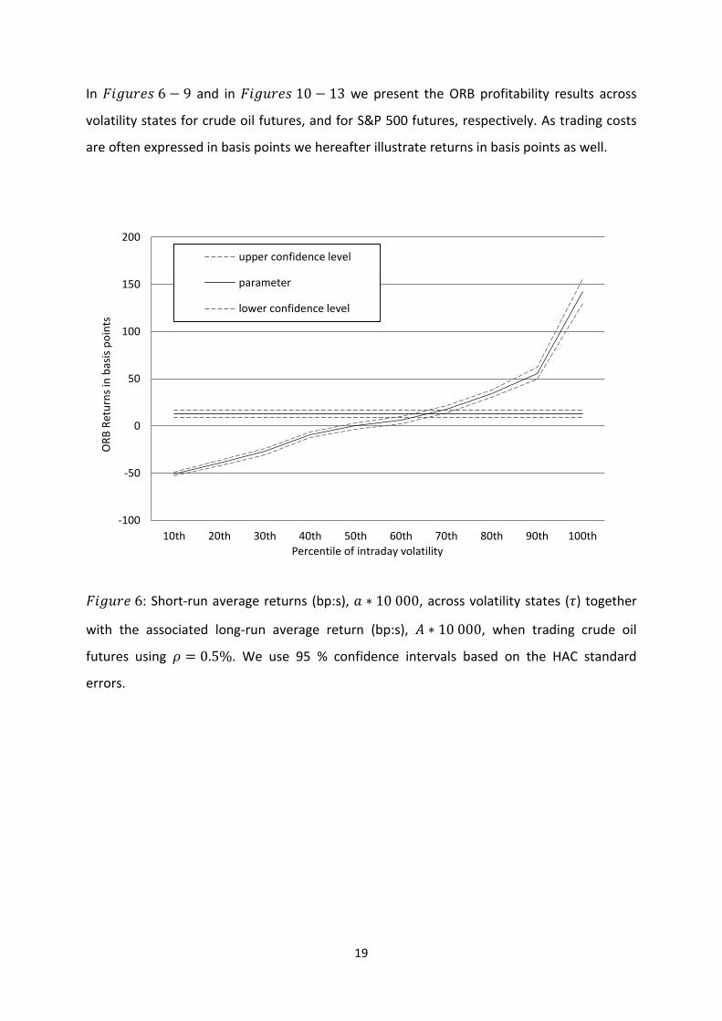
In and in we present the ORB profitability results across
volatility states for crude oil futures, and for S&P 500 futures, respectively. As trading costs
are often expressed in basis points we hereafter illustrate returns in basis points as well.
: Short-run average returns (bp:s), , across volatility states ( ) together
with the associated long-run average return (bp:s), , when trading crude oil
futures using . We use 95 % confidence intervals based on the HAC standard
errors.
-100
-50
0
50
100
150
200
10th 20th 30th 40th 50th 60th 70th 80th 90th 100th
OR
B R
etu
rns
in b
asis
po
ints
Percentile of intraday volatility
upper confidence level
parameter
lower confidence level
20
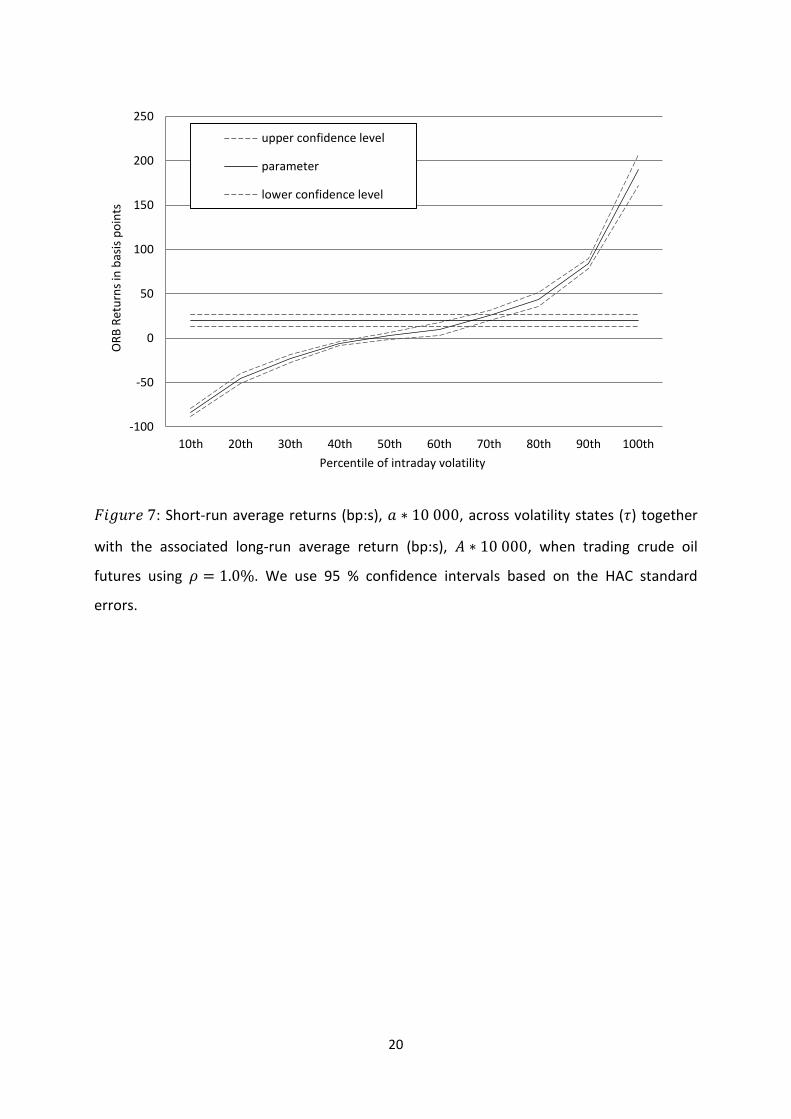
: Short-run average returns (bp:s), , across volatility states ( ) together
with the associated long-run average return (bp:s), , when trading crude oil
futures using . We use 95 % confidence intervals based on the HAC standard
errors.
-100
-50
0
50
100
150
200
250
10th 20th 30th 40th 50th 60th 70th 80th 90th 100th
OR
B R
etu
rns
in b
asis
po
ints
Percentile of intraday volatility
upper confidence level
parameter
lower confidence level
21
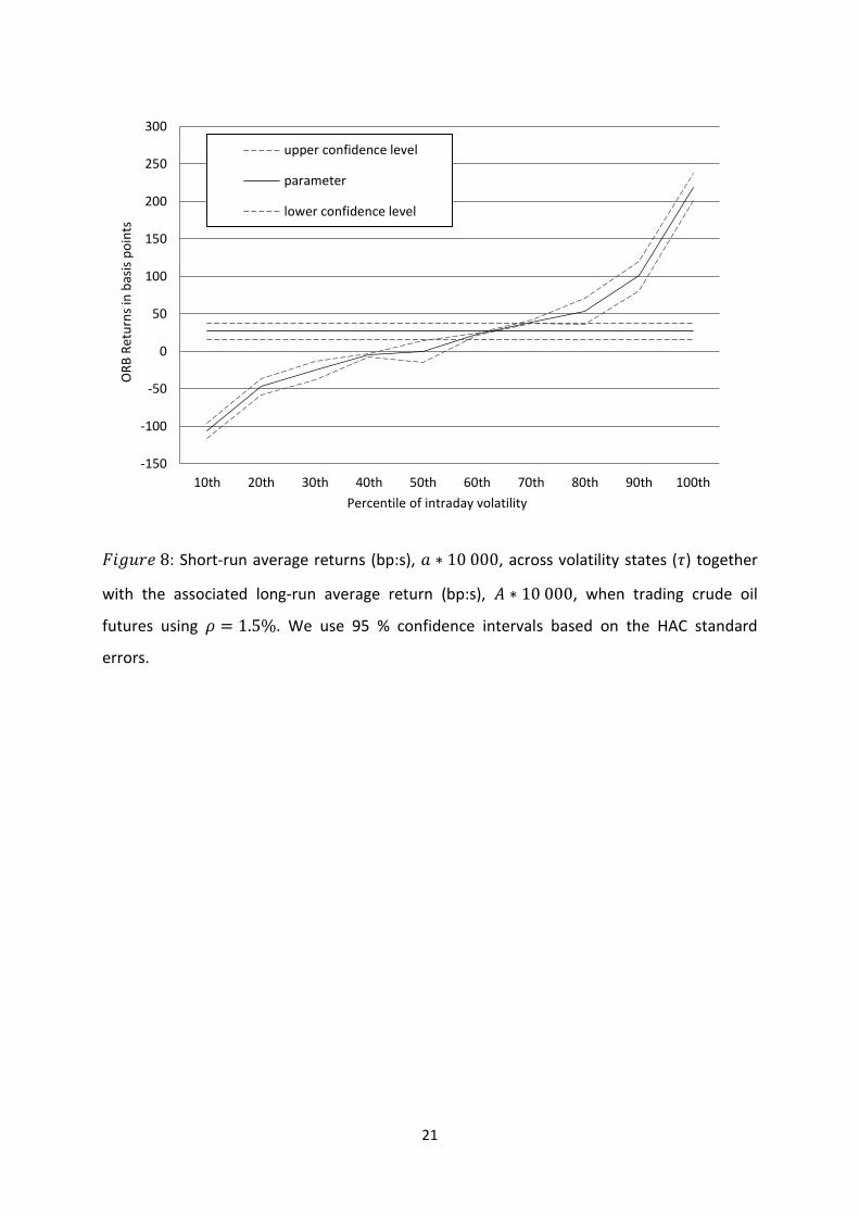
: Short-run average returns (bp:s), , across volatility states ( ) together
with the associated long-run average return (bp:s), , when trading crude oil
futures using . We use 95 % confidence intervals based on the HAC standard
errors.
-150
-100
-50
0
50
100
150
200
250
300
10th 20th 30th 40th 50th 60th 70th 80th 90th 100th
OR
B R
etu
rns
in b
asis
po
ints
Percentile of intraday volatility
upper confidence level
parameter
lower confidence level
22
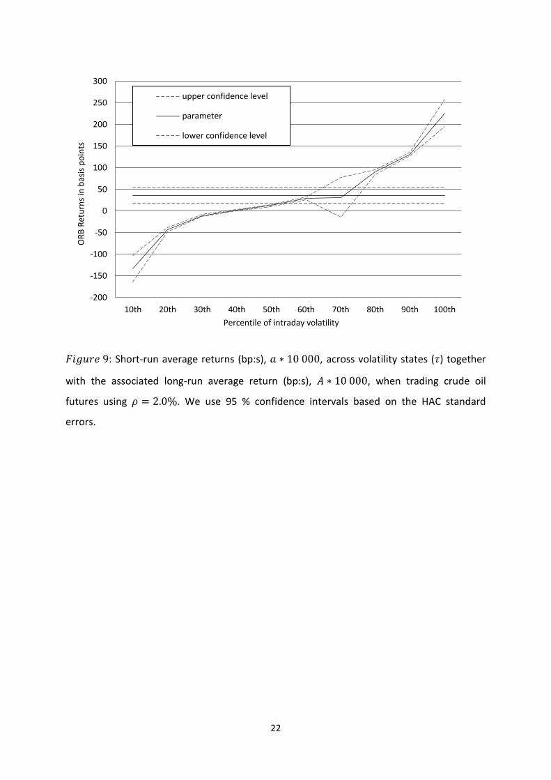
: Short-run average returns (bp:s), , across volatility states ( ) together
with the associated long-run average return (bp:s), , when trading crude oil
futures using . We use 95 % confidence intervals based on the HAC standard
errors.
-200
-150
-100
-50
0
50
100
150
200
250
300
10th 20th 30th 40th 50th 60th 70th 80th 90th 100th
OR
B R
etu
rns
in b
asis
po
ints
Percentile of intraday volatility
upper confidence level
parameter
lower confidence level
23
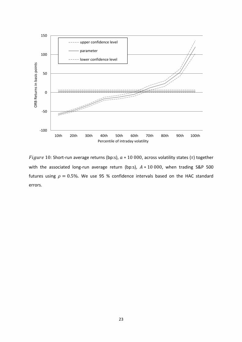
: Short-run average returns (bp:s), , across volatility states ( ) together
with the associated long-run average return (bp:s), , when trading S&P 500
futures using . We use 95 % confidence intervals based on the HAC standard
errors.
-100
-50
0
50
100
150
10th 20th 30th 40th 50th 60th 70th 80th 90th 100th
OR
B R
etu
rns
in b
asis
po
ints
Percentile of intraday volatility
upper confidence level
parameter
lower confidence level

24
: Short-run average returns (bp:s), , across volatility states ( ) together
with the associated long-run average return (bp:s), , when trading S&P 500
futures using . We use 95 % confidence intervals based on the HAC standard
errors.
-150
-100
-50
0
50
100
150
200
250
10th 20th 30th 40th 50th 60th 70th 80th 90th 100th
OR
B R
etu
rns
in b
asis
po
ints
Percentile of intraday volatility
upper confidence level
parameter
lower confidence level

25
: Short-run average returns (bp:s), , across volatility states ( ) together
with the associated long-run average return (bp:s), , when trading S&P 500
futures using . We use 95 % confidence intervals based on the HAC standard
errors.
-150
-100
-50
0
50
100
150
200
250
300
10th 20th 30th 40th 50th 60th 70th 80th 90th 100th
OR
B R
etu
rns
in b
asis
po
ints
Percentile of intraday volatility
upper confidence level
parameter
lower confidence level
26
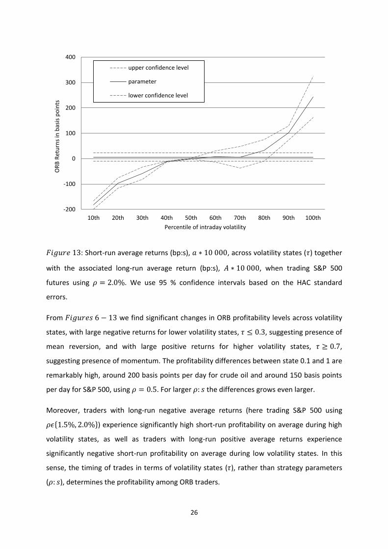
: Short-run average returns (bp:s), , across volatility states ( ) together
with the associated long-run average return (bp:s), , when trading S&P 500
futures using . We use 95 % confidence intervals based on the HAC standard
errors.
From we find significant changes in ORB profitability levels across volatility
states, with large negative returns for lower volatility states, , suggesting presence of
mean reversion, and with large positive returns for higher volatility states, ,
suggesting presence of momentum. The profitability differences between state 0.1 and 1 are
remarkably high, around 200 basis points per day for crude oil and around 150 basis points
per day for S&P 500, using . For larger the differences grows even larger.
Moreover, traders with long-run negative average returns (here trading S&P 500 using
{ }) experience significantly high short-run profitability on average during high
volatility states, as well as traders with long-run positive average returns experience
significantly negative short-run profitability on average during low volatility states. In this
sense, the timing of trades in terms of volatility states ( ), rather than strategy parameters
( ), determines the profitability among ORB traders.
-200
-100
0
100
200
300
400
10th 20th 30th 40th 50th 60th 70th 80th 90th 100th
OR
B R
etu
rns
in b
asis
po
ints
Percentile of intraday volatility
upper confidence level
parameter
lower confidence level
27
As the results up to this point does not include trading costs, and since prices are not always
continuous, even within the trading day (e.g. Mandelbrot, 1963; Fama and Blume, 1966),
actual trading results may differ somewhat from the results we find here.
Admittedly, trading costs in terms of commission fees and bid ask spreads will consume
some of the profits. However, for the assets under consideration during the trading hours of
the US markets, these costs are relatively small. We estimate that for crude oil futures we
need to deduct 4 basis points per trade, or 8 basis points roundtrip daily cost, and for S&P
500 we need to deduct 3 basis points per trade, or 6 basis points roundtrip daily cost,
respectively. We can see from the results in , expressing ORB returns in basis
points, that these costs are in many tests negligible comparing to the size of the profitability
with the lower end of the confidence interval well above a hypothetical level of trading cost.
We recognize, however, that possible discontinuous price jumps will affect the ORB
profitability, but in the case of the ORB strategy not necessarily in a negative way. Prices are
not always continuous, even within a trading day, but experience frequent price jumps in the
direction of the most recent price movement (e.g. Mandelbrot, 1963; Fama and Blume,
1966). Because of the price jumps the trader may experience an order fill at worse prices
than expected, denoted slippage in the trading literature Williams (1999). Consequently,
technical trading rules based on intraday thresholds such as the filter rule of Alexander
(1961) may therefore over-estimate the actual profitability. We first model the slippage
effect in market entries and, second, the slippage effect in market exits;
As price jumps occurs in the direction of the most recent price movement the ORB traders’
entry prices are sometimes filled at some other price than the threshold. If ̃ denotes the
actual entry price during day we may write the slippage effect; ̃
and ̃
,
respectively, based on ̃ where is the size of the price jump. Here slippage
implies a strict negative effect on ORB profitability as long as we assume equal expected
profitability levels for all . For reasonable estimates of when trading commodity
futures, for various trade sizes and for various order execution approaches, see Marshall
(2012).
As ORB traders exit with a time stop, in contrast to exit at a threshold, the direction of
possible price jumps is instead randomly distributed as the prior price movement is no
28
longer clear. If we denote by, ̃ , the actual closing price of day we may write the expected
slippage effect when exit on close; ( ̃ )
.
In contrast to the filter rule of Alexander (1961) where both the market entry and exit are
based on intraday threshold crossing, the ORB strategy is only affected by slippage at the
market entry level. We know, however, that the expected profitability levels differs across
, given by the results in . The total effect of slippage on ORB profitability, taking
both entries and exists into account, can easily be seen for the full sample in or
across volatility states in . We find that the effect of slippage varies among
assets. It is in fact positive in terms of profitability for larger if trading crude oil, while
negative, or positive, depending on the initial level of if trading S&P 500.

29
5. Concluding Discussion
Recent research links the profitability of a popular day trading strategy, the ORB strategy, to
intraday momentum. We illustrated that the expected return of the ORB strategy is
positively related to the intraday volatility of the underlying asset. When applied to long
time series of crude oil futures and to S&P 500 index futures, respectively, we find significant
changes in ORB profitability levels across volatility states. The profitability differences
between the lowest volatility state and the highest volatility state are remarkably high,
around 200 basis points per day for crude oil and around 150 basis points per day for S&P
500.
The main contribution of this paper is that we propose intraday volatility as a factor
generating time-varying market inefficiencies creating intraday profit opportunities for day
traders. We find empirical evidence of intraday momentum in periods of high volatility,
intraday mean reversion in periods of low volatility, and with efficient prices in-between.
From the findings of this paper we may say that the ORB strategy has crises alpha (e.g.
Kaminski, 2011) with increased profitability during market turmoil. We also highlight the
need for using long time series to avoid possible volatility bias when evaluating day trading
profitability, and further, as volatility clusters in financial returns series are somewhat
predictable (e.g. Engle, 1982) we recommend that volatility predictors should be used in day
trading.
30
References
Alexander, S. (1961): “Price Movements in Speculative Markets: Trends or Random Walks,”
Industrial Management Review, 2, 7-26.
Andersen, T.G., and T. Bollerslev (1998): ”Answering the skeptics: Yes, standard volatility
models do provide accurate forecasts,” International Economic Review, 39, 885-905.
Barber, B.M., Y. Lee, Y. Liu, and T. Odean (2006): “Do Individual Day Traders Make Money?
Evidence from Taiwan,” Working Paper. University of California at Davis and Peking
University and University of California, Berkeley.
Barber, B.M., Y. Lee, Y. Liu, and T. Odean (2011): “The cross-section of speculator skill:
Evidence from day trading,” Working Paper. University of California at Davis and Peking
University and University of California, Berkeley.
Barber, B.M., and T. Odean (1999): “The courage of Misguided Convictions.” Financial
Analysts Journal, 55, 41-55.
Barberis, N., A. Shleifer, and R. Vishny (1998): “A Model of Investor Sentiment," Journal of
Financial Economics, 49, 307-343.
Cont, R. (2001): “Empirical properties of asset returns: stylized facts and statistical issues.“
Quantitative Finance, 1, 223-236.
Coval, J.D., D.A. Hirshleifer, and T. Shumway (2005): “Can Individual Investors Beat the
Market?” Working Paper No. 04-025. School of Finance, Harvard University.
Crabel, T. (1990): Day Trading With Short Term Price Patterns Day Trading With Short Term
Price Patterns and Opening Range Breakout, Greenville, S.C.: Traders Press.
Crombez, J. (2001): “Momentum, Rational Agents and Efficient Markets," Journal of
Psychology and Financial Markets, 2, 190-200.
Daniel, K., D. Hirshleifer, and A. Subrahmanyam (1998): “Investor Psychology and Security
Market Under- and Overreactions" Journal of Finance, 53, 1839-1885.
31
Engle, R. F. (1982): “Autoregressive Conditional Heteroscedasticity with Estimates of the
Variance of United Kingdom Inflation," Econometrica, 50.
Fama, E. (1965): “The Behavior of Stock Market Prices," Journal of Business, 38, 34-105.
Fama, E. (1970): “Efficient Capital Markets: A Review of Theory and Empirical Work," The
Journal of Finance, 25, 383-417.
Fama, E. and M. Blume (1966): “Filter Rules and Stock Market Trading Profits," Journal of
Business, 39, 226-241.
Garvey, R. and A. Murphy (2005): “Entry, exit and trading profits: A look at the trading
strategies of a proprietary trading team. Journal of Empirical Finance 12, 629-649.
Harris, J. and P. Schultz (1998): “The trading profits of soes bandits,” Journal of Financial
Economics, 50, 39-62.
Holmberg, U., C. Lonnbark, and C. Lundstrom (2013): ”Assessing the Profitability of Intraday
Opening Range Breakout Strategies,” Finance Research Letters, 10, 27-33.
Jegadeesh, N. and S. Titman (1993): “Returns to Buying Winners and Selling Losers:
Implications for Stock Market Efficiency," Journal of Finance, 48, 65-91.
Jordan, D.J. and D.J. Diltz (2003): “The Profitability of Day Traders,” Financial Analysts
Journal, 59, 85-94.
Kaminski, K. (2011): “Diversifying Risk with Crisis Alpha,” Futures Magazine, February.
Kuo, W-Y. and T-C. Lin (2013): “Overconfident Individual Day Traders: Evidence from the
Taiwan Futures Market,” Journal of Banking & Finance, forthcoming.
Lim, K. and R. Brooks (2011): “The evolution of stock market efficiency over time: a survey of
the empirical literature,” Journal of Economic Surveys, 25, 69-108.
Linnainmaa, J. (2005): “The individual day trader”. Working Paper. University of Chicago.
Lo, A.W. (2004): “The adaptive market hypothesis: market efficiency from an evolutionary
perspective,” Journal of Portfolio Management, 30, 15-29.
32
MacKinnon J.G. and H. White (1985): “Some heteroscedasticity-consistent covariance matrix
estimators with improved finite sample properties,” Journal of Econometrics, 29, 305-325.
Mandelbrot, B. (1963): “The Variation of Certain Speculative Prices.” The Journal of Business
36, 394–419.
Marshall, B.R., R.H. Cahan, and J.M. Cahan (2008): “Can Commodity Futures Be Profitably
Traded with Quantitative Market Timing Strategies?” Journal of Banking & Finance, 32,
1810–1819.
Marshall, B.R., R.H. Cahan, and J.M. Cahan (2008): “Does Intraday Technical Analysis in the
U.S. Equity Market Have Value?” Journal of Empirical Finance, 15, 199–210.
Marshall, B.R., N.H. Nguyen, and N. Visaltanachoti (2012): “Commodity Liquidity
Measurement and Transaction Costs.” Review of Financial Studies, 25, 599–638.
Martens, M., D. van Dijk, and M. de Pooter (2009): “Forecasting S&P 500 Volatility: Long
Memory, Level Shifts, Leverage Effects, Day-of-the-week Seasonality, and Macroeconomic
Announcements.” International Journal of Forecasting, 25, 282–303.
Miffre, J. and G. Rallis (2007): “Momentum Strategies in Commodity Futures Markets,"
Journal of Banking & Finance, 31, 1863-1886.
Park, C. and S.H. Irwin (2007): “What Do We Know About the Profitability of Technical
Analysis?” Journal of Economic Surveys, 21, 786–826.
Pelletier, B. (1997): “Computed Contracts: Computed Contracts: Their Meaning, Purpose and
Application," CSI Technical Journal, 13, 1-6.
Saliba, J., J. Corona, and K. Johnson (2009): Option Spread Strategies: Trading Up, Down, and
Sideways Markets, Bloomberg Press, New York.
Samuelson, P. A. (1965): “Proof That Properly Anticipated Prices Fluctuate Randomly,"
Industrial Management Review, 6, 41-49.
Schulmeister, S. (2009): “Profitability of technical Stock trading: Has it moved from daily to
intraday data?” Review of Financial Economics, 18, 190-201.
33
Self J.K. and I. Mathur (2006): “Asymmetric stationarity in national stock market indices: an
MTAR analysis,” Journal of Business, 79, 3153-74.
Statman, M. (2002): “Lottery Players / Stock Traders,” Financial Analysts Journal. 58, 14-21.
Sullivan, R., A. Timmermann, and H. White (1999): “Data-Snooping, Technical Trading Rule
Performance, and the Bootstrap.” The Journal of Finance, 54, 1647–1691.
White, H. (2000): “A Reality Check for Data Snooping.” Econometrica, 68, 1097–1126.
Williams, L. (1999): Long-Term Secrets to Short-Term Trading, John Wiley & Sons, Inc.,
Hoboken, New Jersey.
Yamamoto, R. (2012): “Intraday Technical Analysis of Individual Stocks on the Tokyo Stock
Exchange.” Journal of Banking & Finance, 36, 3033–3047.