Embed Size (px)
Citation preview

Day 3: Predictive Modeling & Causal Inferences
Beibei Li
Carnegie Mellon University


Day 1: BI & DA Overview, Business Cases - Individual Assignment Day 2: Machine Learning & Data Mining Basics - Group Assignment Day 3: Predictive Modeling vs. Causal Inferences - How to Interpret Regression Results - Causal Identification Strategies; - Economic Value of Online Word-of-Mouth; - Social Network Influence; - Multichannel Advertising Attribution; - Randomized Field Experiment of Mobile Recommendation. Day 4: Bridging Machine Learning with Social Science: - Case 1: Interplay Between Social Media & Search Engine; - Case 2: Understand and Predict Consumer Search and Purchase Behavior; - Case 3: Text Mining & Sponsored Search Advertising.
6

Model-Free Data Exploration & Visualization Unsupervised Learning (Pattern Discovery) (Market Basket Analysis, Association Rule, Clustering)
Supervised Learning (Predictive Modeling) (Decision Tree, Linear Regression, Logistic Regression)
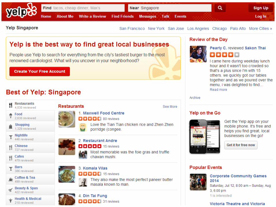
Your brain can efficiently process properly visualized data.
8
9
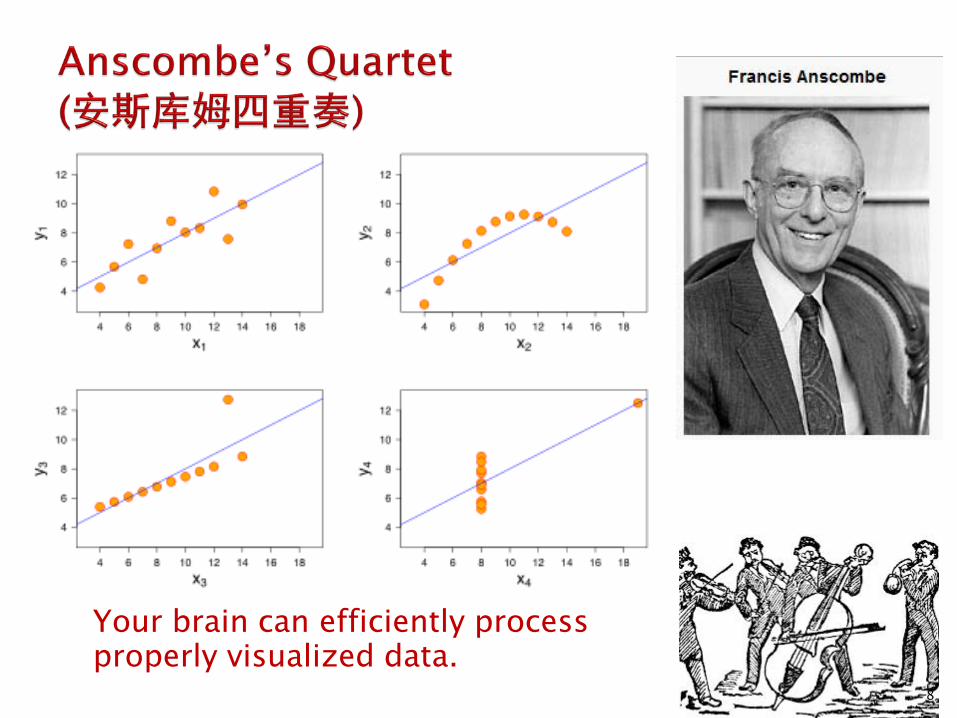
•Market basket Analysis • Most important part of a business: what merchandise
customers are buying and when? •Association Rules
• Building association rules • How good are association rules
•Clustering • Group similar items • Consumer Segmentation

10
Customers tend to buy things together – What can we learn from the basket?
11
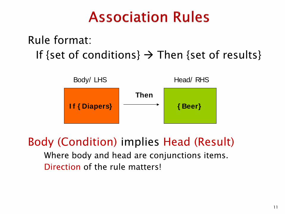
Rule format: If {set of conditions} Then {set of results} Body (Condition) implies Head (Result)
Where body and head are conjunctions items. Direction of the rule matters!
If {Diapers} {Beer} Then
Body/ LHS Head/ RHS

Consider the rule A =>B o Support (“Co-occurrence”)
o Confidence (“Conditional occurrence”)
o Expected Confidence
o Lift
Recap: Association Rule Evaluation Criteria
P(A,B)
P(B|A)
P(B)
P(B|A) P(A,B) P(B) = P(A)P(B)
12

13
•Market basket Analysis • Most important part of a business: what merchandise
customers are buying and when? •Association Rules
• Building association rules • How good are association rules
•Clustering • Group similar items • Consumer Segmentation

Key: What is Similarity?
The quality or state of being similar; likeness; resemblance; as, a similarity of features. -- Webster's Dictionary

15
case gender glasses Moustache smile hat
1 0 1 0 1 0
2 1 0 0 1 0
3 0 1 0 0 0
4 0 0 0 0 0
5 0 0 0 1 0
6 0 0 1 0 1
7 0 1 0 1 0
8 0 0 0 1 0
9 0 1 1 1 0
10 1 0 0 0 0
11 0 0 1 0 0
12 1 0 0 0 0
Each user is represented as a “feature vector”

16
Need a distance measure for different cases (ectors)
Example for a distance measure: the Euclidean distance.
∑=
−=n
iii yxYXD
1
2)(),(
X = [x1 x2 x3 x4 x5 …] Y = [y1 y2 y3 y4 y5 …]
case gender glasses Moustache smile hat
1 0 1 0 1 0
2 1 0 0 1 0
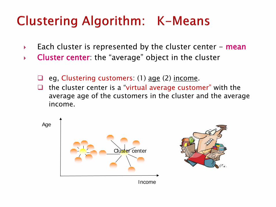
Each cluster is represented by the cluster center - mean Cluster center: the “average” object in the cluster
eg, Clustering customers: (1) age (2) income. the cluster center is a “virtual average customer” with the
average age of the customers in the cluster and the average income.
Income
Age
Cluster center

18
Market basket Analysis • Most important part of a business: what merchandise
customers are buying and when? Association Rules
• Building association rules • How good are association rules
Clustering • Group similar items • Consumer Segmentation

Model-Free Data Exploration & Visualization Unsupervised Learning (Pattern Discovery) (Market Basket Analysis, Association Rule, Clustering)
Supervised Learning (Predictive Modeling) (Decision Tree, Linear Regression, Logistic Regression)

Predictive Modeling Needs Model Validation!
Too few parameters Too many parameters

Overfitting Problem

Overfitting Problem
Model training should stop here!

23
Prediction Overview Classification (vs. Regression)
Decision Trees Regression
• Linear Regression • Logistic Regression
Naive Bayes SVM K-Nearest Neighbor (KNN) …

- An upside-down tree

Balance<50K
Balance>=50K
16 bad 14 good
4 bad 13 good
12 bad 1 good
Age<45
Age>=45
16 bad 14 good
3 bad 11 good
13 bad 3 good
Which Attribute to Choose?

Purity Measures: ◦ Gini (population diversity)
◦ Entropy (information gain)
◦ Chi-square Test

27
Entropy and Information Gain Entropy How mixed/noisy is a set? (“uncertainty”) -Originally defined to account for the flow of energy through a thermodynamic process.
Assume there are two classes, Pink and Green When the set of examples S contain p elements of class Pink and g elements of class Green
Information Grain Expected reduction in entropy. e.g., How much closer to purity?
2 2( ) log logp p g gE Sp g p g p g p g
= − − + + + +
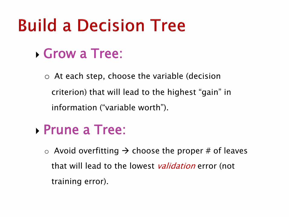
Grow a Tree: o At each step, choose the variable (decision
criterion) that will lead to the highest “gain” in
information (“variable worth”).
Prune a Tree: o Avoid overfitting choose the proper # of leaves
that will lead to the lowest validation error (not
training error).

Form a group of 4-6; Write a summary report about the major
methodologies of machine learning methods, including both supervised and unsupervised learning;
Compare the pros and cons for each method; Find a real-world business application of each
method you discuss; Page limit 5-10 pages, in English; Due: Last day of class.
29
30
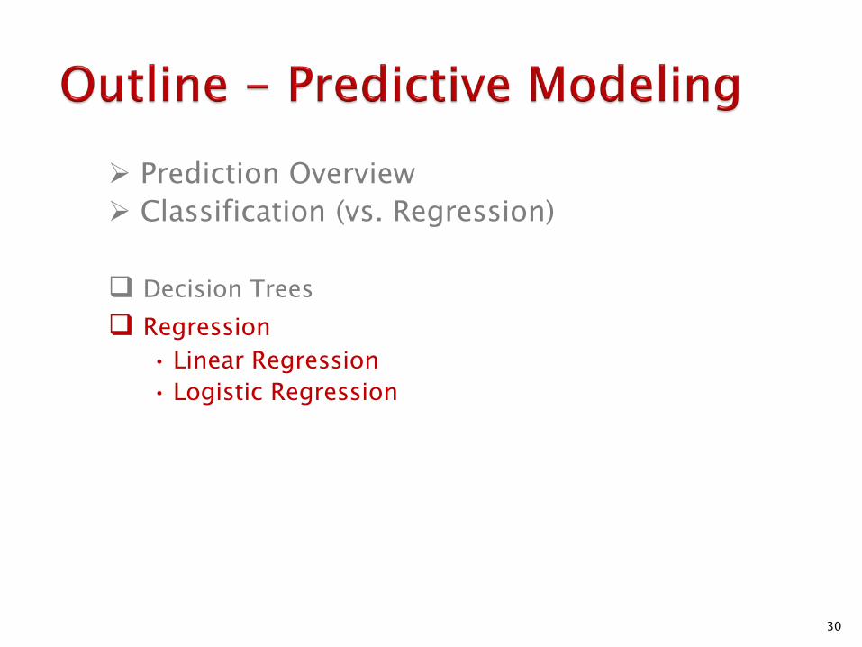
Prediction Overview Classification (vs. Regression)
Decision Trees Regression
• Linear Regression • Logistic Regression
31
Regression Linear Regression (线性回归) Logistic Regression (逻辑回归)
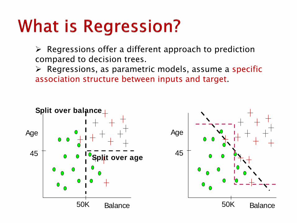
Regressions offer a different approach to prediction compared to decision trees. Regressions, as parametric models, assume a specific association structure between inputs and target.
Balance
Age
Split over age
Split over balance
50K
45
Balance
Age
50K
45

Linear relationship: Outcome (dependent/criterion) variable is a linear combination of predictor (independent) variables.
In two dimensions (one predictor, one outcome variable) data can be plotted on a scatter diagram.
y = β0 + β1 x + ε
Expected value of y (outcome)
Intercept Term coefficient
Predictor variable

Regression Model y = β0 + β1x +ε
Unknown Parameters β0, β1
Sample Data: x y
x1 y1 . .
. . xn yn
b0 and b1 provide estimates of
β0 and β1
Estimated Regression Equation
Sample Statistics
b0, b1
0 1y b b x= +

E(y): Outcome
x : Predictor
Slope b1 positive
Regression line
Intercept b0
Y

E(y): Outcome
x: Predictor
Slope b1 negative
Regression line Intercept b0
Simple Linear Regression Equation:

Y
X
Y
X
Y
Y
X
X
A “linear” model means linear in Parameters (not x)

•
• • •
• • •
•
• •
•
•
• •
• •
• •
•
•
• •
•
•
•
• •
•
•
•
E(y)
x
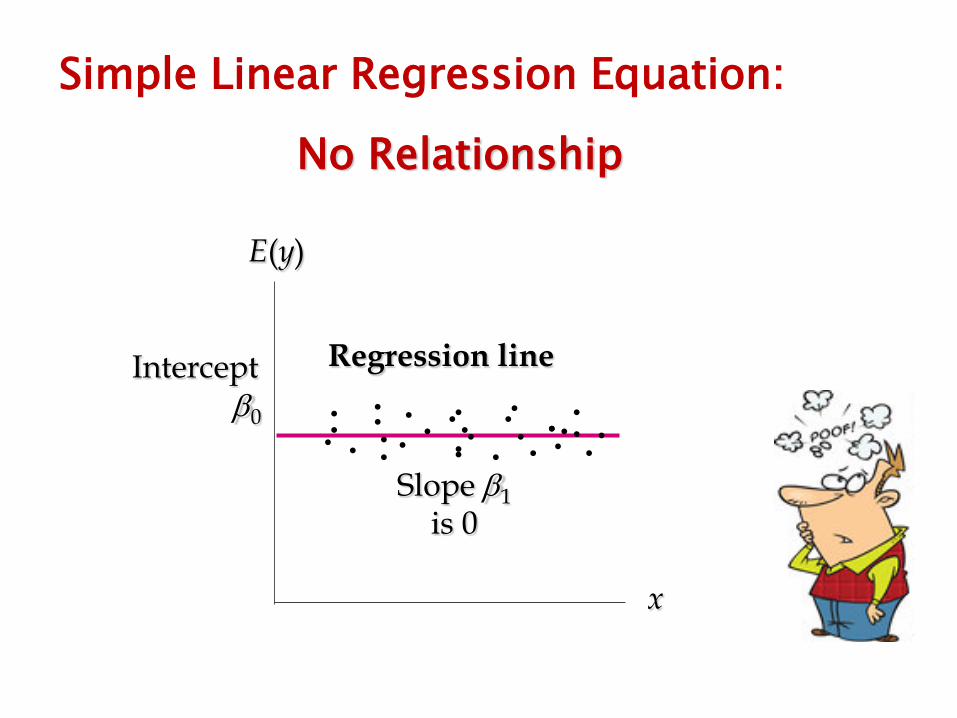
Slope β1 is 0
Regression line Intercept β0
Simple Linear Regression Equation: No Relationship
E(y)
x
Slope β1 is 0
Regression line Intercept β0
• • • • • • •
• • • •
• • • • • • • • •
• • • •
• • • • •
•
Simple Linear Regression Equation: No Relationship

Y
X
Y
X
Y
Y
X
X
Strong relationships Weak relationships
How to evaluate?
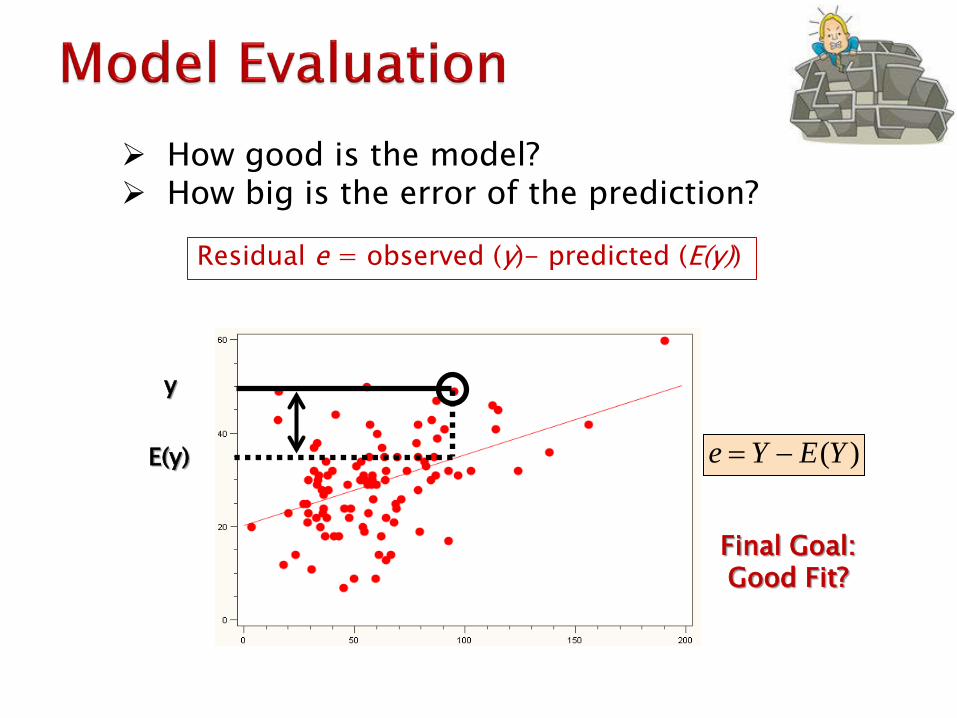
How good is the model? How big is the error of the prediction?
Residual e = observed (y)- predicted (E(y))
y
E(y) ( )e Y E Y= −
Final Goal: Good Fit?
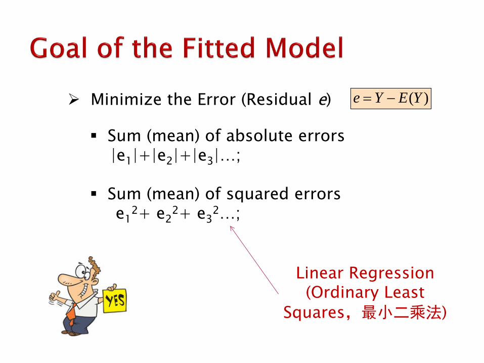
Minimize the Error (Residual e)
Sum (mean) of absolute errors |e1|+|e2|+|e3|…; Sum (mean) of squared errors e1
2+ e22+ e3
2…;
Linear Regression (Ordinary Least
Squares,最小二乘法)
( )e Y E Y= −

Predicted Line
Actual Data
Least Squares Criterion: minimize sum of squared errors (vertical distance between actual data & estimated line)
^ 2min ( )i iy yn
−∑

b1 - Slope for the Estimated Regression Equation
b0 - Intercept for the Estimated Regression Equation
0 1b y b x= −
where: xi = value of independent variable for i-th observation
n = total number of observations
_ y = mean value for dependent variable
_ x = mean value for independent variable
yi = value of dependent variable for i-th observation
− −=
−
∑∑1 2
( )( )
( )
i in
in
x x y yb
x x

More than one predictor…
E(y)= α + β1*X + β2 *W + β3 *Z… Each regression coefficient is the amount of change
in the outcome variable that would be expected per one-unit change of the predictor, if all other variables in the model were held constant.
Market Share = α + β1*Price + β2 * Rating + β3 *#Reviews…

eg. Buy vs. No buy? What is the probability for a consumer to buy a product? – Can we use simple Linear Regression?
0 ≤ Pr(x) ≤ 1
Bounded by 0 and 1 Nonlinear
-- Need proper transformation!

Similar to linear regression, two main differences: Y (outcome or response) is binary Yes/No Approve/Reject Responded/Did not respond
Result is expressed as a probability of being in either group.
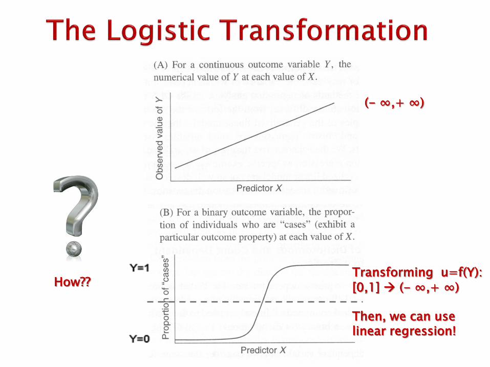
Transforming u=f(Y): [0,1] (- ∞,+ ∞) Then, we can use linear regression!
How??
(- ∞,+ ∞)
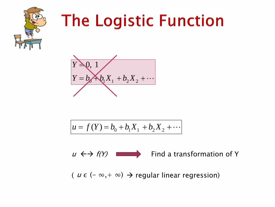
0 1 1 2 2( )u f Y b b X b X= = + + +
0 1 1 2 2
0, 1YY b b X b X
=
= + + +
u f(Y) Find a transformation of Y ( regular linear regression)
u ∊ (- ∞,+ ∞)

Probability of Success (Odds): - probability of success for case i.
ˆ ( 1| ) 1
u
ueP Y X
eπ = = =
+
π[0,1]
Odds-Ratio for Success: Ratio of the probability of success over the probability of failure.
ˆ ( 1| ) ˆ(1 ) ( 0 | )
uP Y XP Y X
eππ
== = − =
(0,+∞)
“Logit”: Log Odds-Ratio, taking the natural log of both sides, we can write the Logistic regression equation as
For Each Case i: (u regular linear regression)
: (), ( ) ( , ).Goal Find f so that u f Y= ∈ −∞ +∞
0 1 1 2 2ˆ ( 1| )ln ln ...
ˆ(1 ) ( 0 | )P Y X u b b X b XP Y X
ππ
== = = + + + − =
(- ∞,+∞)
f(Y)
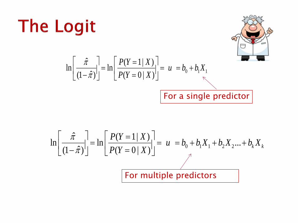
0 1 1ˆ ( 1| )ln ln
ˆ(1 ) ( 0 | )P Y X u b b XP Y X
ππ
== = = + − =
For a single predictor
0 1 1 2 2ˆ ( 1| )ln ln ...
ˆ(1 ) ( 0 | ) k kP Y X u b b X b X b XP Y X
ππ
== = = + + + − =
For multiple predictors

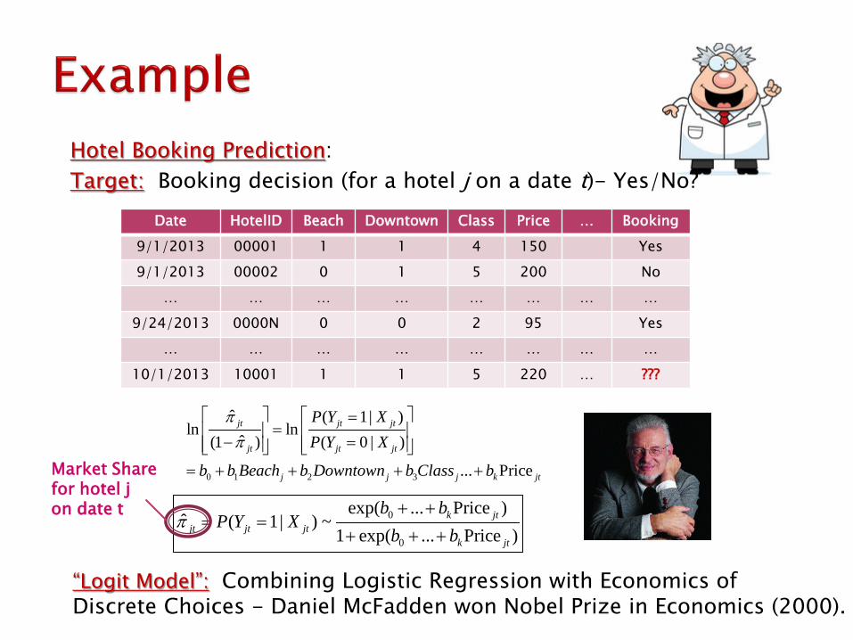
Hotel Booking Prediction: • Hotel A, $150 per night, 4-class, near beach, downtown, … • Hotel B, $200 per night, 5-class, near highway, swimming pool,… • … • Hotel N, … Target: Booking decision (for a hotel j on a date t)- Yes/No?
Date HotelID Beach Downtown Class Price … Booking 9/1/2013 00001 1 1 4 150 Yes 9/1/2013 00002 0 1 5 200 No
… … … … … … … … 9/24/2013 0000N 0 0 2 95 Yes
… … … … … … … … 10/1/2013 10001 1 1 5 220 … ???
0
0
exp( ... Price )ˆ ( 1| ) ~
1 exp( ... Price )k jt
jt jt jtk jt
b bP Y X
b bπ
+ += =
+ + +
0 1 2 3
ˆ ( 1| )ln ln
ˆ(1 ) ( 0 | )
... Price
jt jt jt
jt jt jt
j j j k jt
P Y XP Y X
b b Beach b Downtown b Class b
ππ
==
− = = + + + +
Hotel Booking Prediction: Target: Booking decision (for a hotel j on a date t)- Yes/No?
Market Share for hotel j on date t
“Logit Model”: Combining Logistic Regression with Economics of Discrete Choices - Daniel McFadden won Nobel Prize in Economics (2000).
Date HotelID Beach Downtown Class Price … Booking 9/1/2013 00001 1 1 4 150 Yes 9/1/2013 00002 0 1 5 200 No
… … … … … … … … 9/24/2013 0000N 0 0 2 95 Yes
… … … … … … … … 10/1/2013 10001 1 1 5 220 … ???

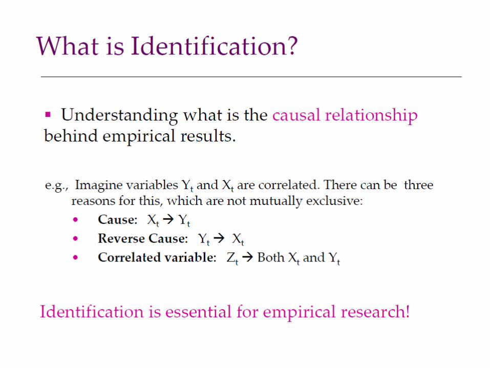
Interpretation of Regression - Be Careful!
How to Interpret Regression Results? Causal Effect Identification Strategies; Economic Value of Online Word-of-Mouth; Social Network Influences; Multichannel Advertising Attribution; Randomized Field Experiments of Mobile Recommendations;
Interpretation of Regression - Be Careful!
How to Interpret Regression Results? Causal Effect Identification Strategies; Economic Value of Online Word-of-Mouth; Social Network Influences; Multichannel Advertising Attribution; Randomized Field Experiments of Mobile Recommendations;
56
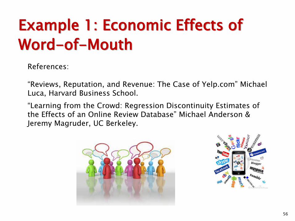
Example 1: Economic Effects of Word-of-Mouth
References: “Reviews, Reputation, and Revenue: The Case of Yelp.com” Michael Luca, Harvard Business School. “Learning from the Crowd: Regression Discontinuity Estimates of the Effects of an Online Review Database” Michael Anderson & Jeremy Magruder, UC Berkeley.

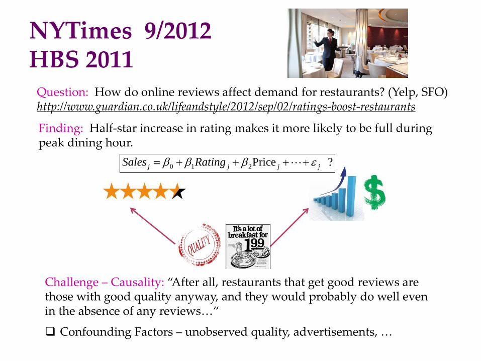
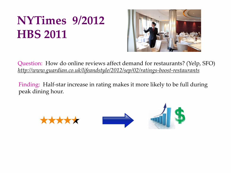
NYTimes 9/2012 HBS 2011
Question: How do online reviews affect demand for restaurants? (Yelp, SFO) http://www.guardian.co.uk/lifeandstyle/2012/sep/02/ratings-boost-restaurants
Finding: Half-star increase in rating makes it more likely to be full during peak dining hour.
Challenge – Causality: “After all, restaurants that get good reviews are those with good quality anyway, and they would probably do well even in the absence of any reviews…“
Confounding Factors – unobserved quality, advertisements, …
0 1 2Price ?j j j jSales Ratingβ β β ε= + + + +


NYTimes/HBS

Regression Discontinuity Identifying Causality: “Rounding Mechanism” on Social Media Websites

Any potential issues?

Gaming the reputation system?
Self-select?
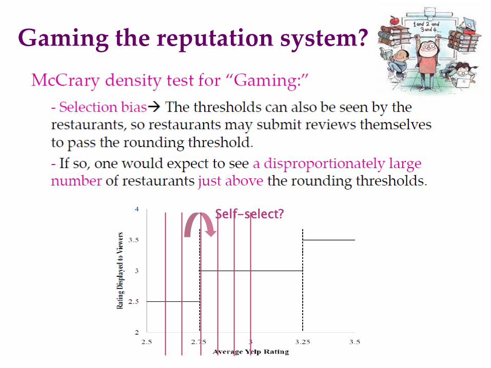
Gaming the reputation system?
Self-select?
NYTimes 9/2012 HBS 2011
Question: How do online reviews affect demand for restaurants? (Yelp, SFO) http://www.guardian.co.uk/lifeandstyle/2012/sep/02/ratings-boost-restaurants
Finding: Half-star increase in rating makes it more likely to be full during peak dining hour.
67
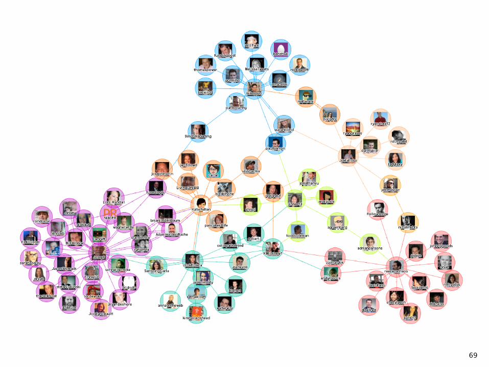
Example 2: Social Network Influence

68
69
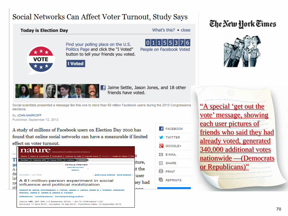
70
“A special ‘get out the vote’ message, showing each user pictures of friends who said they had already voted, generated 340,000 additional votes nationwide —(Democrats or Republicans)”

71
72
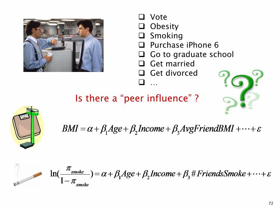
Vote Obesity Smoking Purchase iPhone 6 Go to graduate school Get married Get divorced …
Is there a “peer influence” ?

73
Regression tells you only “correlation”
The causality is not clear…
How to identify the causal influence?
74
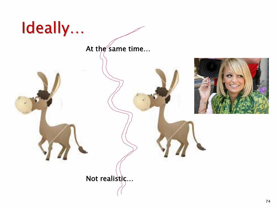
Ideally… At the same time…
Not realistic…

75
Matching At the same time…
76
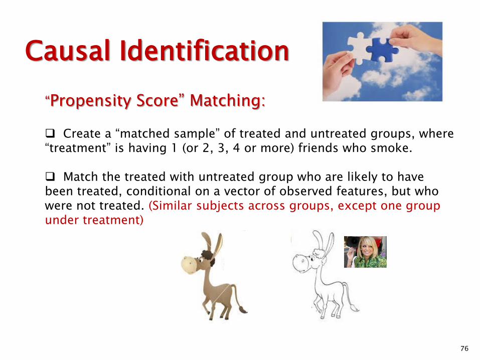
Causal Identification “Propensity Score” Matching: Create a “matched sample” of treated and untreated groups, where “treatment” is having 1 (or 2, 3, 4 or more) friends who smoke.
Match the treated with untreated group who are likely to have been treated, conditional on a vector of observed features, but who were not treated. (Similar subjects across groups, except one group under treatment)
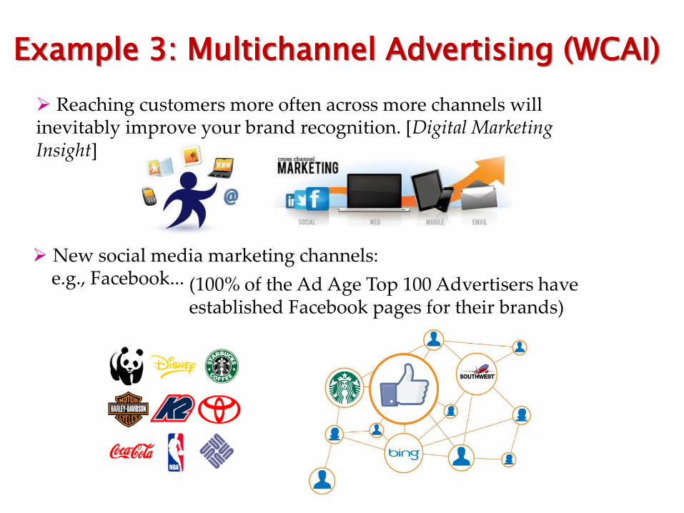
Reaching customers more often across more channels will inevitably improve your brand recognition. [Digital Marketing Insight]
New social media marketing channels: e.g., Facebook... (100% of the Ad Age Top 100 Advertisers have
established Facebook pages for their brands)
Example 3: Multichannel Advertising (WCAI)

Brands can attract hundreds, thousands, or even millions of “LIKEs” on FB.
HERSHEY'S: 6,037,545 likes Coca-Cola: 72,299,176 likes Disney: 45,049,811 likes Nike: 15,327,236 likes ……
Example 3: Multichannel Advertising

Are the fans really fans?
Do FB LIKEs/brand exposure lead to more sales?
Starbucks Fans: 4.2 times more likely to visit Starbucks.com; Southwest Fans: 3.6 times more likely to visit Southwest.com. - comScore (2011)
Example 3: Multichannel Advertising

o Audience self-selection (e.g., being targeted or clicking “LIKE” due to inherent brand affinity)
o Other unobserved confounding factors
Lack of effective metrics in measuring brand advertising effects
Causal effect identification
Bias the estimated effect of marketing effort.

Overlapping of advertising campaigns from other media channels;
e.g., TV advertising, online display ads… Multiple media channels tend to largely interact with
each other.
Bias the estimated effect of marketing effort.
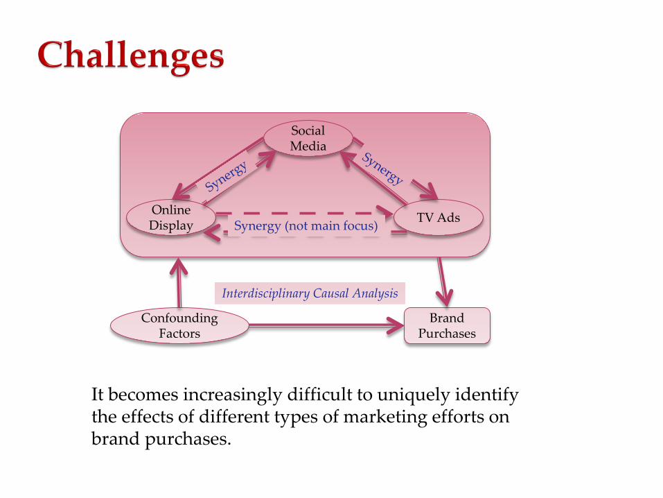
It becomes increasingly difficult to uniquely identify the effects of different types of marketing efforts on brand purchases.
Brand Purchases
Confounding Factors
Social Media
Online Display TV Ads Synergy (not main focus)
Interdisciplinary Causal Analysis
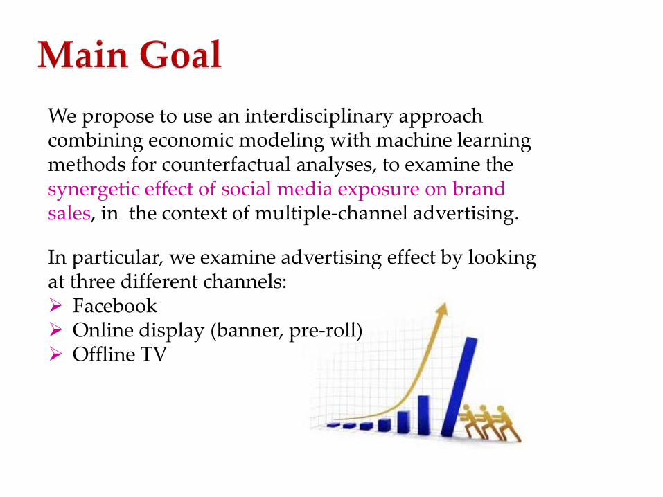
We propose to use an interdisciplinary approach combining economic modeling with machine learning methods for counterfactual analyses, to examine the synergetic effect of social media exposure on brand sales, in the context of multiple-channel advertising. In particular, we examine advertising effect by looking at three different channels: Facebook Online display (banner, pre-roll) Offline TV
84
• 12 months panel (2011/1/1-2011/12/31) • FB, online, TV, purchase, sociodemographics • Both categories, both sponsor’s umbrands and competitors’ umbrands • Leading to 4 umbrands. • Goal: Daily FB exposure brand purchases in next 30 days.
Example 3: Multichannel Advertising
85
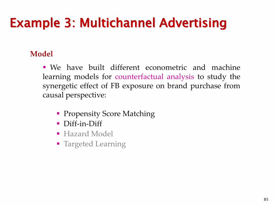
We have built different econometric and machine learning models for counterfactual analysis to study the synergetic effect of FB exposure on brand purchase from causal perspective:
Propensity Score Matching Diff-in-Diff Hazard Model Targeted Learning
Example 3: Multichannel Advertising

86
At the same time…
How to find match?

First, we use a propensity score matching (PSM) approach, where we match customers based on Socio-demographic attributes; TV ads exposure ; Online display ads exposure;
87
The idea is to simulate a randomized experiment -- an controlled group and a treatment group, with the same predicted propensity of getting treated (i.e., FB exposure).
However, the only difference between the two groups is that one is treated, whereas the other is not.

Based on the matched samples, we use a diff-in-diff model to control for both time-invariant and time-varying unobserved factors.
First-level difference: Monitor changes in brand sales over time for each group group-fixed effect
Second-level difference: Monitor discrepancy in the above changes between the two groups group-time fixed effect
88

89
We find if we consider all the four brands and estimation the overall FB effect, the estimates are insignificant.
Our guess – FB exposure may have different effects on sales for different brands.
Therefore, we further break down and look into individual brand separately.
90
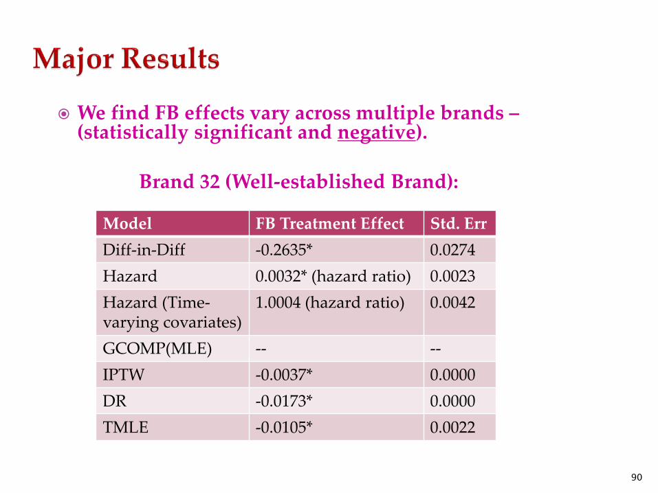
Model FB Treatment Effect Std. Err Diff-in-Diff -0.2635* 0.0274 Hazard 0.0032* (hazard ratio) 0.0023 Hazard (Time-varying covariates)
1.0004 (hazard ratio) 0.0042
GCOMP(MLE) -- -- IPTW -0.0037* 0.0000 DR -0.0173* 0.0000 TMLE -0.0105* 0.0022
We find FB effects vary across multiple brands –(statistically significant and negative).
Brand 32 (Well-established Brand):

91
Model FB Treatment Effect Std. Err Diff-in-Diff 0.1933* 0.0041 Hazard 1.0168* (hazard ratio) 0.0005 Hazard (Time-varying covariates)
1.0112 (hazard ratio) 0.0061
GCOMP(MLE) -- -- IPTW 0.2575* 0.0000 DR 0.2019* 0.0000 TMLE 0.1821* 0.0012
We find FB effects vary across multiple brands –(statistically significant and positive).
Brand 73 (New, Less-established Brand):
92
FB exposure has statistically significant effects on brand sales
on certain brands (not all). However, it seems the efforts are not significant in magnitude.
Effects of FB exposure vary across brands. (Not always positive! – May depend on the brand page activities.)
Negative FB effect exists on next-30-day purchase for certain (more well-known/established) brands.
Traditional advertising channels (TV/Online) have larger effects than FB.
In general, findings are highly consistent across multiple causal analytical models.
93
We have tried # of Exposures (and log version as well) rather than
a binary indicator for each type of exposure (FB/Online/TV);
We have broken down different types of FB exposure (owned/earned), different types of online exposure (banner/pre-roll/FB banner);
We have tried different sliding time windows for purchase measurement (next 1, 3, 7, 14, 30 days);
Example 3: Multichannel Advertising

94
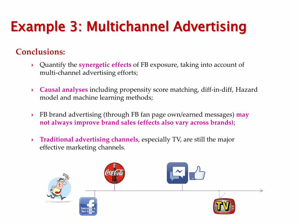
Quantify the synergetic effects of FB exposure, taking into account of multi-channel advertising efforts;
Causal analyses including propensity score matching, diff-in-diff, Hazard model and machine learning methods;
FB brand advertising (through FB fan page own/earned messages) may not always improve brand sales (effects also vary across brands);
Traditional advertising channels, especially TV, are still the major effective marketing channels.
Example 3: Multichannel Advertising

96
Causal Identification “Propensity Score” Matching: Create a “matched sample” of treated and untreated groups, where “treatment” is having 1 (or 2, 3, 4 or more) friends who smoke.
Match the treated with untreated group who are likely to have been treated, conditional on a vector of observed features, but who were not treated. (Similar subjects across groups, except one group under treatment)
Need Data!
97
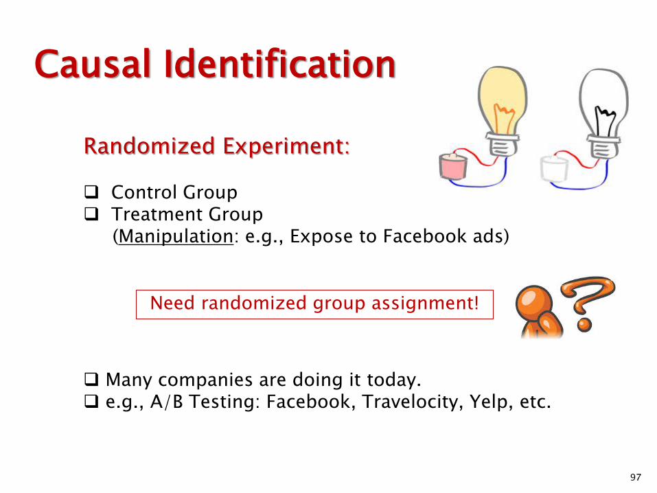
Causal Identification
Randomized Experiment: Control Group Treatment Group (Manipulation: e.g., Expose to Facebook ads)
Need randomized group assignment!
Many companies are doing it today. e.g., A/B Testing: Facebook, Travelocity, Yelp, etc.

98
Example 4: Randomized Field Experiments
Business Question:
How Effective is Mobile Recommendation?

A major large shopping mall in Beijing ◦ 120,000 square meters ◦ 100,000 visitors per day; 200,000 visitors per day during
holidays ◦ WiFi localization system ◦ 300+ stores
Example 4: Randomized Field Experiments

Group 0: Randomly select 1000 consumers, do nothing, observe
Group 1: Randomly select 2000 consumers, send random store sale information
Group 2: Pure location-based recommendation ◦ Send store promotion messages to randomly selected 2000
consumers based on purely real-time location. Group 3: Trajectory-based recommendation ◦ Send promotion messages to randomly selected 2000
consumers based on our recommendation system.
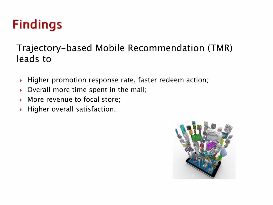
Trajectory-based Mobile Recommendation (TMR) leads to
Higher promotion response rate, faster redeem action; Overall more time spent in the mall; More revenue to focal store; Higher overall satisfaction.

How to Interpret Regression Results? Causal Effect Identification Strategies; Economic Value of Online Word-of-Mouth; Social Network Influences; Multichannel Advertising Attribution; Randomized Field Experiments of Mobile Recommendations;
Regression is very useful in making predictions.
But, Interpretation of Regression
- Be Careful!
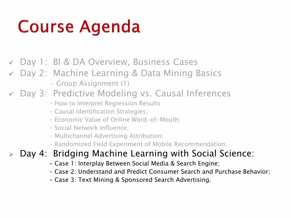
Day 1: BI & DA Overview, Business Cases Day 2: Machine Learning & Data Mining Basics - Group Assignment (1) Day 3: Predictive Modeling vs. Causal Inferences - How to Interpret Regression Results - Causal Identification Strategies; - Economic Value of Online Word-of-Mouth; - Social Network Influence; - Multichannel Advertising Attribution; - Randomized Field Experiment of Mobile Recommendation. Day 4: Bridging Machine Learning with Social Science: - Case 1: Interplay Between Social Media & Search Engine; - Case 2: Understand and Predict Consumer Search and Purchase Behavior; - Case 3: Text Mining & Sponsored Search Advertising.