Nonparametrically Consistent

Depth-based Classifiers

Davy Paindaveine∗ and Germain Van Bever

Universite Libre de Bruxelles, Brussels, Belgium

Abstract

We introduce a class of depth-based classification procedures that are of

a nearest-neighbor nature. Depth, after symmetrization, indeed provides the

center-outward ordering that is necessary and sufficient to define nearest neigh-

bors. The resulting classifiers are affine-invariant and inherit the nonparamet-

ric validity from nearest-neighbor classifiers. In particular, we prove that the

proposed depth-based classifiers are consistent under very mild conditions. We

investigate their finite-sample performances through simulations and show that

they outperform affine-invariant nearest-neighbor classifiers obtained through

an obvious standardization construction. We illustrate the practical value of

our classifiers on two real data examples. Finally, we shortly discuss the possible

uses of our depth-based neighbors in other inference problems.

Keywords and phrases: Affine-invariance, Classification procedures, Nearest Neigh-

bors, Statistical depth functions, Symmetrization.

∗Davy Paindaveine is Professor of Statistics, Universite Libre de Bruxelles, ECARES and

Departement de Mathematique, Avenue F. D. Roosevelt, 50, CP 114/04, B-1050 Bruxelles, Belgium

(E-mail: dpaindav@ulb.ac.be). He is also member of ECORE, the association between CORE and

ECARES. Germain Van Bever is FNRS PhD candidate, Universite Libre de Bruxelles, ECARES

and Departement de Mathematique, Campus de la Plaine, Boulevard du Triomphe, CP 210, B-1050

Bruxelles, Belgium (E-mail: gvbever@ulb.ac.be). This work was supported by an A.R.C. contract

and a FNRS Aspirant contract, Communaute francaise de Belgique.

1

arX

iv:1

204.

2996

v1 [

mat

h.ST

] 1

3 A

pr 2

012

1 INTRODUCTION

The main focus of this work is on the standard classification setup in which the

observation, of the form (X, Y ), is a random vector taking values in Rd × {0, 1}. A

classifier is a function m : Rd → {0, 1} that associates with any value x a predictor

for the corresponding “class” Y . Denoting by IA the indicator function of the set A,

the so-called Bayes classifier, defined through

mBayes(x) = I[η(x) > 1/2

], with η(x) = P [Y = 1 |X = x], (1.1)

is optimal in the sense that it minimizes the probability of misclassification P [m(X) 6=

Y ]. Under absolute continuity assumptions, the Bayes rule rewrites

mBayes(x) = I[f1(x)

f0(x)>π0

π1

], (1.2)

where πj = P [Y = j] and fj denotes the pdf of X conditional on [Y = j]. Of

course, empirical classifiers m(n) are obtained from i.i.d. copies (Xi, Yi), i = 1, . . . , n,

of (X, Y ), and it is desirable that such classifiers are consistent, in the sense that,

as n → ∞, the probability of misclassification of m(n), conditional on (Xi, Yi),

i = 1, . . . , n, converges in probability to the probability of misclassification of the

Bayes rule. If this convergence holds irrespective of the distribution of (X, Y ), the

consistency is said to be universal.

Classically, parametric approaches assume that the conditional distribution of X

given [Y = j] is multinormal with mean µµµj and covariance matrix ΣΣΣj (j = 0, 1).

This gives rise to the so-called quadratic discriminant analysis (QDA)—or to linear

discriminant analysis (LDA) if it is further assumed that ΣΣΣ0 = ΣΣΣ1. It is standard

to estimate the parameters µµµj and ΣΣΣj (j = 0, 1) by the corresponding sample means

and empirical covariance matrices, but the use of more robust estimators was recom-

mended in many works; see, e.g., Randles et al. (1978), He and Fung (2000), Dehon

2

and Croux (2001), or Hartikainen and Oja (2006). Irrespective of the estimators used,

however, these classifiers fail to be consistent away from the multinormal case.

Denoting by dΣΣΣ(x,µµµ) = ((x − µµµ)′ΣΣΣ−1(x − µµµ))1/2 the Mahalanobis distance be-

tween x and µµµ in the metric associated with the symmetric and positive definite

matrix ΣΣΣ, it is well known that the QDA classifier rewrites

mQDA(x) = I[dΣΣΣ1(x,µµµ1) < dΣΣΣ0(x,µµµ0) + C

], (1.3)

where the constant C depends on ΣΣΣ0, ΣΣΣ1, and π0, hence classifies x into Population 1

if it is sufficiently more central in Population 1 than in Population 0 (centrality,

in elliptical setups, being therefore measured with respect to the geometry of the

underlying equidensity contours). This suggests that statistical depth functions, that

are mappings of the form x 7→ D(x, P ) indicating how central x is with respect to a

probability measure P (see Section 2.1 for a more precise definition), are appropriate

tools to perform nonparametric classification. Indeed, denoting by Pj the probability

measure associated with Population j (j = 0, 1), (1.3) makes it natural to consider

classifiers of the form

mD(x) = I[D(x, P1) > D(x, P0)

],

based on some fixed statistical depth function D. This max-depth approach was first

proposed in Liu et al. (1999) and was then investigated in Ghosh and Chaudhuri

(2005b). Dutta and Ghosh (2012a,b) considered max-depth classifiers based on the

projection depth and on (an affine-invariant version of) the Lp depth, respectively.

Hubert and Van der Veeken (2010) modified the max-depth approach based on pro-

jection depth to better cope with possibly skewed data.

Recently, Li et al. (2012) proposed the “Depth vs Depth” (DD) classifiers that ex-

tend the max-depth ones by constructing appropriate polynomial separating curves

in the DD-plot, that is, in the scatter plot of the points (D(n)0 (Xi), D

(n)1 (Xi)), i =

3

1, . . . , n, where D(n)j (Xi) refers to the depth of Xi with respect to the data points

coming from Population j. Those separating curves are chosen to minimize the em-

pirical misclassification rate on the training sample and their polynomial degree m is

chosen through cross-validation. Lange et al. (2012) defined modified DD-classifiers

that are computationally efficient and apply in higher dimensions (up to d = 20).

Other depth-based classifiers were proposed in Jornsten (2004), Ghosh and Chaud-

huri (2005a), and Cui et al. (2008).

Being based on depth, these classifiers are clearly of a nonparametric nature. An

important requirement in nonparametric classification, however, is that consistency

holds as broadly as possible and, in particular, does not require “structural” distri-

butional assumptions. In that respect, the depth-based classifiers available in the

literature are not so satisfactory, since they are at best consistent under elliptical

distributions only1. This restricted-to-ellipticity consistency implies that, as far as

consistency is concerned, the Mahalanobis depth is perfectly sufficient and is by now

means inferior to the “more nonparametric” (Tukey (1975)) halfspace depth or (Liu

(1990)) simplicial depth, despite the fact that it uninspiringly leads to LDA through

the max-depth approach. Also, even this restricted consistency often requires esti-

mating densities; see, e.g., Dutta and Ghosh (2012a,b). This is somewhat undesirable

since density and depth are quite antinomic in spirit (a deepest point may very well

be a point where the density vanishes). Actually, if densities are to be estimated in

the procedure anyway, then it would be more natural to go for density estimation all

the way, that is, to plug density estimators in (1.2).

The poor consistency of the available depth-based classifiers actually follows from

their global nature. Zakai and Ritov (2009) indeed proved that any universally consis-

1The classifiers from Dutta and Ghosh (2012b) are an exception that slightly extends consistency

to (a subset of) the class of Lp-elliptical distributions.

4

tent classifier needs to be of a local nature. In this paper, we therefore introduce local

depth-based classifiers, that rely on nearest-neighbor ideas (kernel density techniques

should be avoided, since, as mentioned above, depth and densities are somewhat in-

compatible). From their nearest-neighbor nature, they will inherit consistency under

very mild conditions, while from their depth nature, they will inherit affine-invariance

and robustness, two important features in multivariate statistics and in classification

in particular. Identifying nearest neighbors through depth will be achieved via an

original symmetrization construction. The corresponding depth-based neighborhoods

are of a nonparametric nature and the good finite-sample behavior of the resulting

classifiers most likely results from their data-driven adaptive nature.

The outline of the paper is as follows. In Section 2, we first recall the concept

of statistical depth functions (Section 2.1) and then describe our symmetrization

construction that allows to define the depth-based neighbors to be used later for clas-

sification purposes (Section 2.2). In Section 3, we define the proposed depth-based

nearest-neighbor classifiers and present some of their basic properties (Section 3.1)

before providing consistency results (Section 3.2). In Section 4, Monte Carlo sim-

ulations are used to compare the finite-sample performances of our classifiers with

those of their competitors. In Section 5, we show the practical value of the proposed

classifiers on two real-data examples. We then discuss in Section 6 some further

applications of our depth-based neighborhoods. Finally, the Appendix collects the

technical proofs.

2 DEPTH-BASED NEIGHBORS

In this section, we review the concept of statistical depth functions and define the

depth-based neighborhoods on which the proposed nearest-neighbor classifiers will be

based.

5

2.1 Statistical depth functions

Statistical depth functions allow to measure centrality of any x ∈ Rd with respect

to a probability measure P over Rd (the larger the depth of x, the more central x is

with respect to P ). Following Zuo and Serfling (2000a), we define a statistical depth

function as a bounded mapping D( ·, P ) from Rd to R+ that satisfies the following

four properties:

(P1) affine-invariance: for any d × d invertible matrix A, any d-vector b and any

distribution P over Rd, D(Ax + b, PA,b) = D(x, P ), where PA,b is defined

through PA,b[B] = P [A−1(B − b)] for any d-dimensional Borel set B;

(P2) maximality at center: for any P that is symmetric about θθθ (in the sense2

that P [θθθ + B] = P [θθθ − B] for any d-dimensional Borel set B), D(θθθ, P ) =

supx∈Rd D(x, P );

(P3) monotonicity relative to the deepest point: for any P having deepest point θθθ,

D(x, P ) ≤ D((1− λ)θθθ + λx, P ) for any x ∈ Rd and any λ ∈ [0, 1];

(P4) vanishing at infinity: for any P , D(x, P )→ 0 as ‖x‖ → ∞.

For any statistical depth function and any α > 0, the set Rα(P ) = {x ∈ Rd :

D(x, P ) ≥ α} is called the depth region of order α. These regions are nested, and,

clearly, inner regions collect points with larger depth. Below, it will often be conve-

nient to rather index these regions by their probability content : for any β ∈ [0, 1),

we will denote by Rβ(P ) the smallest Rα(P ) that has P -probability larger than or

equal to β. Throughout, subscripts and superscripts for depth regions are used for

depth levels and probability contents, respectively.

2Zuo and Serfling (2000a) also considers more general symmetry concepts; however, we restrict

in the sequel to central symmetry, that will be the right concept for our purposes.

6

Celebrated instances of statistical depth functions include

(i) the Tukey (1975) halfspace depth DH(x, P ) = infu∈Sd−1 P [u′(X − x) ≥ 0],

where Sd−1 = {u ∈ Rd : ‖u‖ = 1} is the unit sphere in Rd;

(ii) the Liu (1990) simplicial depth DS(x, P ) = P [x ∈ S(X1,X2, . . . ,Xd+1)], where

S(x1,x2, . . . ,xd+1) denotes the closed simplex with vertices x1,x2, . . . , xd+1 and

where X1,X2, . . . ,Xd+1 are i.i.d. P ;

(iii) the Mahalanobis depth DM(x, P ) = 1/(1 + d2ΣΣΣ(P )(x,µµµ(P ))), for some affine-

equivariant location and scatter functionals µµµ(P ) and ΣΣΣ(P );

(iv) the projection depthDPr(x, P ) = 1/(1+supu∈Sd−1 |u′x−µ(P[u])|/σ(P[u])), where

P[u] denotes the probability distribution of u′X when X ∼ P and where µ(P )

and σ(P ) are univariate location and scale functionals, respectively.

Other depth functions are the simplicial volume depth, the spatial depth, the Lp

depth, etc. Of course, not all such depths fulfill Properties (P1)-(P4) for any dis-

tribution P ; see Zuo and Serfling (2000a). A further concept of depth, of a slightly

different (L2) nature, is the so-called zonoid depth; see Koshevoy and Mosler (1997).

Of course, if d-variate observations X1, . . . ,Xn are available, then sample versions

of the depths above are simply obtained by replacing P with the corresponding empir-

ical distribution P (n) (the sample simplicial depth then has a U -statistic structure).

A crucial fact for our purposes is that a sample depth provides a center-outward

ordering of the observations with respect to the corresponding deepest point θθθ(n)

:

one may indeed order the Xi’s in such a way that

D(X(1), P(n)) ≥ D(X(2), P

(n)) ≥ . . . ≥ D(X(n), P(n)). (2.1)

Neglecting possible ties, this states that, in the depth sense, X(1) is the observation

closest to θθθ(n)

, X(2) the second closest, . . . , and X(n) the one farthest away from θθθ(n)

.

7

For most classical depths, there may be infinitely many deepest points, that form

a convex region in Rd. This will not be an issue in this work, since the symmetrization

construction we will introduce, jointly with Properties (Q2)-(Q3) below, asymptot-

ically guarantee unicity of the deepest point. For some particular depth functions,

unicity may even hold for finite samples: for instance, in the case of halfspace depth,

it follows from Rousseeuw and Struyf (2004) and results on the uniqueness of the

symmetry center (Serfling (2006)) that, under the assumption that the parent distri-

bution admits a density, symmetrization implies almost sure unicity of the deepest

point.

2.2 Depth-based neighborhoods

A statistical depth function, through (2.1), can be used to define neighbors of the deep-

est point θθθ(n)

. Implementing a nearest-neighbor classifier, however, requires defining

neighbors of any point x ∈ Rd. Property (P2) provides the key to the construction

of an x-outward ordering of the observations, hence to the definition of depth-based

neighbors of x : symmetrization with respect to x.

More precisely, we propose to consider depth with respect to the empirical dis-

tribution P(n)x associated with the sample obtained by adding to the original ob-

servations X1,X2, . . . ,Xn their reflections 2x −X1, . . . , 2x −Xn with respect to x.

Property (P2) implies that x is the—unique (at least asymptotically; see above)—

deepest point with respect to P(n)x . Consequently, this symmetrization construction,

parallel to (2.1), leads to an (x-outward) ordering of the form

D(Xx,(1), P(n)x ) ≥ D(Xx,(2), P

(n)x ) ≥ . . . ≥ D(Xx,(n), P

(n)x ).

Note that the reflected observations are only used to define the ordering but are not

ordered themselves. For any k ∈ {1, . . . , n}, this allows to identify—up to possible

8

ties—the k nearest neighbors Xx,(i), i = 1, . . . , k, of x. In the univariate case (d = 1),

these k neighbors coincide—irrespective of the statistical depth function D—with the

k data points minimizing the usual distances |Xi − x|, i = 1, . . . , n.

In the sequel, the corresponding depth-based neighborhoods—that is, the sample

depth regions R(n)x,α = Rα(P

(n)x )—will play an important role. In accordance with

the notation from the previous section, we will write Rβ(n)x for the smallest depth

region R(n)x,α that contains at least a proportion β of the data points X1,X2, . . . ,Xn.

For β = k/n, Rβ(n)x is therefore the smallest depth-based neighborhood that contains k

of the Xi’s; ties may imply that the number of data points in this neigborhood, Kβ(n)x

say, is strictly larger than k.

Note that a distance (or pseudo-distance) (x,y) 7→ d(x,y) that is symmetric in its

arguments is not needed to identify nearest neighbors of x. For that purpose, a col-

lection of “distances” y 7→ dx(y) from a fixed point is indeed sufficient (in particular,

it is irrelevant that this distance satisfies or not the triangular inequality). In that

sense, the (data-driven) symmetric distance associated with the Oja and Paindaveine

(2005) lift-interdirections, that was recently used to build nearest-neighbor regression

estimators in Biau et al. (2012), is unnecessarily strong. Also, only an ordering of the

“distances” is needed to identify nearest neighbors. This ordering of distances from a

fixed point x is exactly what the depth-based x-outward ordering above is providing.

3 DEPTH-BASED kNN CLASSIFIERS

In this section, we first define the proposed depth-based classifiers and present some

of their basic properties (Section 3.1). We then state the main result of this paper,

related to their consistency properties (Section 3.2).

9

3.1 Definition and basic properties

The standard k-nearest-neighbor (kNN) procedure classifies the point x into Popula-

tion 1 iff there are more observations from Population 1 than from Population 0 in the

smallest Euclidean ball centered at x that contains k data points. Depth-based kNN

classifiers are naturally obtained by replacing these Euclidean neighborhoods with the

depth-based neighborhoods introduced above, that is, the proposed kNN procedure

classifies x into Population 1 iff there are more observations from Population 1 than

from Population 0 in the smallest depth-based neighborhood of x that contains k

observations—i.e., in Rβ(n)x , β = k/n. In other words, the proposed depth-based

classifier is defined as

m(n)D (x) = I

[∑ni=1I[Yi = 1]W

β(n)i (x) >

∑ni=1 I[Yi = 0]W

β(n)i (x)

], (3.1)

with Wβ(n)i (x) = 1

Kβ(n)x

I[Xi ∈ Rβ(n)x ], where K

β(n)x =

∑nj=1 I[Xj ∈ Rβ(n)

x ] still denotes

the number of observations in the depth-based neighborhood Rβ(n)x . Since

m(n)D (x) = I

[η

(n)D (x) > 1/2

], with η

(n)D (x) =

∑ni=1I[Yi = 1]W

β(n)i (x), (3.2)

the proposed classifier is actually the one obtained by plugging, in (1.1), the depth-

based estimator η(n)D (x) of the conditional expectation η(x). This will be used in

the proof of Theorem 3.1 below. Note that in the univariate case (d = 1), m(n)D ,

irrespective of the statistical depth function D, reduces to the standard (Euclidean)

kNN classifier.

It directly follows from Property (P1) that the proposed classifier is affine-invariant,

in the sense that the outcome of the classification will not be affected if X1, . . . ,Xn

and x are subject to a common (arbitrary) affine transformation. This clearly im-

proves over the standard kNN procedure that, e.g., is sensitive to unit changes. Of

course, one natural way to define an affine-invariant kNN classifier is to apply the orig-

10

inal kNN procedure on the standardized data points ΣΣΣ−1/2

Xi, i = 1, . . . , n, where ΣΣΣ

is an affine-equivariant estimator of shape—in the sense that

ΣΣΣ(AX1 + b, . . . ,AXn + b) ∝ AΣΣΣ(X1, . . . ,Xn)A′

for any invertible d × d matrix A and any d-vector b. A natural choice for ΣΣΣ is the

regular covariance matrix, but more robust choices, such as, e.g., the shape estimators

from Tyler (1987), Dumbgen (1998), or Hettmansperger and Randles (2002) would

allow to get rid of any moment assumption. Here, we stress that, unlike our adaptive

depth-based methodology, such a transformation approach leads to neighborhoods

that do not exploit the geometry of the distribution in the vicinity of the point x to

be classified (these neighborhoods indeed all are ellipsoids with x-independent orienta-

tion and shape); as we show through simulations below, this results into significantly

worse performances.

The main depth-based classifiers available—among which those relying on the

max-depth approach of Liu et al. (1999) and Ghosh and Chaudhuri (2005b), as well as

the more efficient ones from Li et al. (2012)—suffer from the “outsider problem3” : if

the point x to be classified does not sit in the convex hull of any of the two populations,

then most statistical depth functions will give x zero depth with respect to each

population, so that x cannot be classified through depth. This is of course undesirable,

all the more so that such a point x may very well be easy to classify. To improve

on this, Hoberg and Mosler (2006) proposed extending the original depth fields by

using the Mahalanobis depth outside the supports of both populations, a solution

that quite unnaturally requires combining two depth functions. Quite interestingly,

our symmetrization construction implies that the depth-based kNN classifier (that

involves one depth function only) does not suffer from the outsider problem; this is

an important advantage over competing depth-based classifiers.

3The term “outsider” was recently introduced in Lange et al. (2012).

11

While our depth-based classifiers in (3.1) are perfectly well-defined and enjoy, as

we will show in Section 3.2 below, excellent consistency properties, practitioners might

find quite arbitrary that a point x such that∑n

i=1I[Yi = 1]Wβ(n)i (x) =

∑ni=1 I[Yi =

0]Wβ(n)i (x) is assigned to Population 0. Parallel to the standard kNN classifier, the

classification may alternatively be based on the population of the next neighbor. Since

ties are likely to occur when using depth, it is natural to rather base classification

on the proportion of data points from each population in the next depth region.

Of course, if the next depth region still leads to an ex-aequo, the outcome of the

classification is to be determined on the subsequent depth regions, until a decision

is reached (in the unlikely case that an ex-aequo occurs for all depth regions to be

considered, classification should then be done by flipping a coin). This treatment of

ties is used whenever real or simulated data are considered below.

Finally, practitioners have to choose some value for the smoothing parameter kn.

This may be done, e.g., through cross-validation (as we will do in the real data

example of Section 5). The value of kn is likely to have a strong impact on finite-

sample performances, as confirmed in the simulations we conduct in Section 4.

3.2 Consistency results

As expected, the local (nearest-neighbor) nature of the proposed classifiers makes

them consistent under very mild conditions. This, however, requires that the statis-

tical depth function D satisfies the following further properties:

(Q1) continuity: if P is symmetric about θθθ and admits a density that is positive at θθθ

and continuous in a neighborhood of θθθ, then x 7→ D(x, P ) is continuous in a

neighborhood of θθθ.

(Q2) unique maximization at the symmetry center: if P is symmetric about θθθ and

12

admits a density that is positive at θθθ and continuous in a neighborhood of θθθ,

then D(θθθ, P ) > D(x, P ) for all x 6= θθθ.

(Q3) consistency: for any bounded d-dimensional Borel set B, supx∈B |D(x, P (n))−

D(x, P )| = o(1) almost surely as n → ∞, where P (n) denotes the empirical

distribution associated with n random vectors that are i.i.d. P .

Property (Q2) complements Property (P2), and, in view of Property (P3), only

further requires that θθθ is a strict local maximizer of x 7→ D(x, P ). Note that Prop-

erties (Q1)-(Q2) jointly ensure that the depth-based neighborhoods of x from Sec-

tion 2.2 collapse to the singleton {x} when the depth level increases to its maximal

value. Finally, since our goal is to prove that our classifier satisfies an asymptotic

property (namely, consistency), it is not surprising that we need to control the asymp-

totic behavior of the sample depth itself (Property (Q3)). As shown by Theorem A.1

in the Appendix, Properties (Q1)-(Q3) are satisfied for many classical depth func-

tions.

We can then state the main result of the paper.

Theorem 3.1 Let D be a depth function satisfying (P2), (P3) and (Q1)-(Q3). Let kn

be a sequence of positive integers such that kn →∞ and kn = o(n) as n→∞. Assume

that, for j = 0, 1, X|[Y = j] admits a density fj whose collection of discontinuity

points is closed and has Lebesgue measure zero. Then the depth-based knNN classifier

m(n)D in (3.1) is consistent in the sense that

P [m(n)D (X) 6= Y | Dn]− P [mBayes(X) 6= Y ] = oP (1) as n→∞,

where Dn is the sigma-algebra associated with (Xi, Yi), i = 1, . . . , n.

Classically, consistency results for classification are based on a famous theorem

from Stone (1977); see, e.g., Theorem 6.3 in Devroye et al. (1996). However, it is an

13

open question whether Condition (i) of this theorem holds or not for the proposed clas-

sifiers, at least for some particular statistical depth functions. A sufficient condition

for Condition (i) is actually that there exists a partition of Rd into cones C1, . . . , Cγd

with vertex at the origin of Rd (γd not depending on n) such that, for any Xi and

any j, there exist (with probability one) at most k data points X` ∈ Xi + Cj that

have Xi among their k depth-based nearest neighbors. Would this be established for

some statistical depth function D, it would prove that the corresponding depth-based

knNN classifier m(n)D is universally consistent, in the sense that consistency holds

without any assumption on the distribution of (X, Y ).

Now, it is clear from the proof of Stone’s theorem that this condition (i) may be

dropped if one further assumes that X admits a uniformly continuous density. This

is however a high price to pay, and that is the reason why the proof of Theorem 3.1

rather relies on an argument recently used in Biau et al. (2012); see the Appendix.

4 SIMULATIONS

We performed simulations in order to evaluate the finite-sample performances of the

proposed depth-based kNN classifiers. We considered six setups, focusing on bivariate

Xi’s (d = 2) with equal a priori probabilities (π0 = π1 = 1/2), and involving the

following densities f0 and f1:

Setup 1 (multinormality) fj, j = 0, 1, is the pdf of the bivariate normal distribution

with mean vector µµµj and covariance matrix ΣΣΣj, where

µµµ0 =(

0

0

), µµµ1 =

(1

1

), ΣΣΣ0 =

(1 1

1 4

), ΣΣΣ1 = 4ΣΣΣ0;

Setup 2 (bivariate Cauchy) fj, j = 0, 1, is the pdf of the bivariate Cauchy distribution

with location center µµµj and scatter matrix ΣΣΣj, with the same values of µµµj and ΣΣΣj

14

as in Setup 1;

Setup 3 (flat covariance structures) fj, j = 0, 1, is the pdf of the bivariate normal

distribution with mean vector µµµj and covariance matrix ΣΣΣj, where

µµµ0 =(

0

0

), µµµ1 =

(1

1

), ΣΣΣ0 =

(52 0

0 1

), ΣΣΣ1 = ΣΣΣ0;

Setup 4 (uniform distributions on half-moons) f0 and f1 are the densities of

(X

Y

)=(U

V

)and

(X

Y

)=( −0.5

2

)+(

1 0.5

0.5 −1

)(U

V

),

respectively, where U ∼ Unif(−1, 1) and V |[U = u] ∼ Unif(1− u2, 2(1− u2));

Setup 5 (uniform distributions on rings) f0 and f1 are the uniform distributions on the

concentric rings {x ∈ R2 : 1 ≤ ‖x‖ ≤ 2} and {x ∈ R2 : 1.75 ≤ ‖x‖ ≤ 2.5},

respectively;

Setup 6 (bimodal populations) fj, j = 0, 1, is the pdf of the multinormal mixture

12N (µµµIj ,ΣΣΣ

Ij ) + 1

2N (µµµIIj ,ΣΣΣ

IIj ), where

µµµI0 =(

0

0

), µµµII0 =

(3

3

), ΣΣΣI

0 =(

1 1

1 4

), ΣΣΣII

0 = 4ΣΣΣI0,

µµµI1 =(

1.5

1.5

), µµµII1 =

(4.5

4.5

), ΣΣΣI

1 =(

4 0

0 0.5

), and ΣΣΣII

1 =(

0.75 0

0 5

).

For each of these six setups, we generated 250 training and test samples of

size n = ntrain = 200 and ntest = 100, respectively, and evaluated the misclassifi-

cation frequencies of the following classifiers:

1. the usual LDA and QDA classifiers (LDA/QDA);

2. the standard Euclidean kNN classifiers (kNN), with β = k/n = 0.01, 0.05,

0.10 and 0.40, and the corresponding “Mahalanobis” kNN classifiers (kNNaff)

15

obtained by performing the Euclidean kNN classifiers on standardized data,

where standardization is based on the regular covariance matrix estimate of the

pooled training sample;

3. the proposed depth-based kNN classifiers (D-kNN) for each combination of the

k used in kNN/kNNaff and a statistical depth function (we focused on halfspace

depth, simplicial depth, or Mahalanobis depth);

4. the depth vs depth (DD) classifiers from Li et al. (2012), for each combina-

tion of a polynomial curve of degree m (m = 1, 2, or 3) and a statistical

depth function (halfspace depth, simplicial depth, or Mahalanobis depth). Ex-

act DD-classifiers (DD) as well as smoothed versions (DDsm) were actually

implemented —although, for computational reasons, only the smoothed version

was considered for m = 3. Exact classifiers search for the best separating poly-

nomial curve (d, r(d)) of order m passing through the origin and m “DD-points”

(D(n)0 (Xi), D

(n)1 (Xi)) (see the Introduction) in the sense that it minimizes the

missclassification error

n∑i=1

(I[Yi = 1]I[d(n)

i > 0] + I[Yi = 0]I[−d(n)i > 0]

), (4.1)

with d(n)i := r(D

(n)0 (Xi)) − D(n)

1 (Xi). Smoothed versions use derivative-based

methods to find a polynomial minimizing (4.1), where the indicator I[d > 0] is

replaced by the logistic function 1/(1 + e−td) for a suitable t. As suggested in

Li et al. (2012), value t = 100 was chosen in these simulations. 100 randomly

chosen polynomials were used as starting points for the minimization algorithm,

the classifier using the resulting polynomial with minimal misclassification (note

that this time-consuming scheme always results into better performances than

the one adopted in Li et al. (2012), where only one minimization is performed,

starting from the best random polynomial considered).

16

Since the DD classification procedure is a refinement of the max-depth procedures

of Ghosh and Chaudhuri (2005b) that leads to better misclassification rates (see Li

et al. (2012)), the original max-depth procedures were omitted in this study.

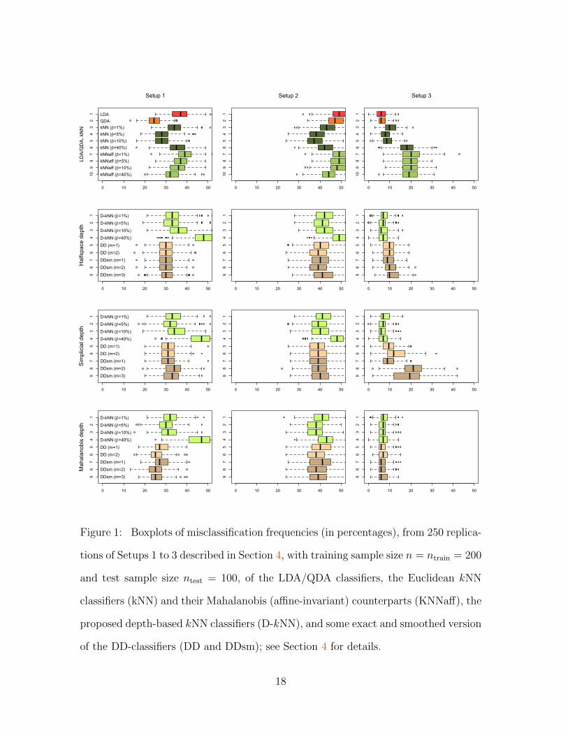
Boxplots of misclassification frequencies (in percentages) are reported in Figures 1

and 2. The main learnings from these simulations are the following:

• In most setups, the proposed depth-based kNN classifiers compete well with the

Euclidean kNN classifiers and improve over the latter under the flat covariance

structures in Setup 3. This may be attributed to the lack of affine-invariance of

the Euclidean kNN classifiers, which leads to discard this procedure and rather

focus on its affine-invariant version (kNNaff). It is very interesting to note

that the kNNaff classifiers in most cases are outperformed by the depth-based

kNN classifiers. In other words, the natural way to make the standard kNN

classifier affine-invariant results into a dramatic cost in terms of finite-sample

performances. Incidentally, we point out that, in some setups, the choice of the

smoothing parameter kn appears to have less impact on affine-invariant kNN

procedures than on the original kNN procedures; see, e.g., Setup 3.

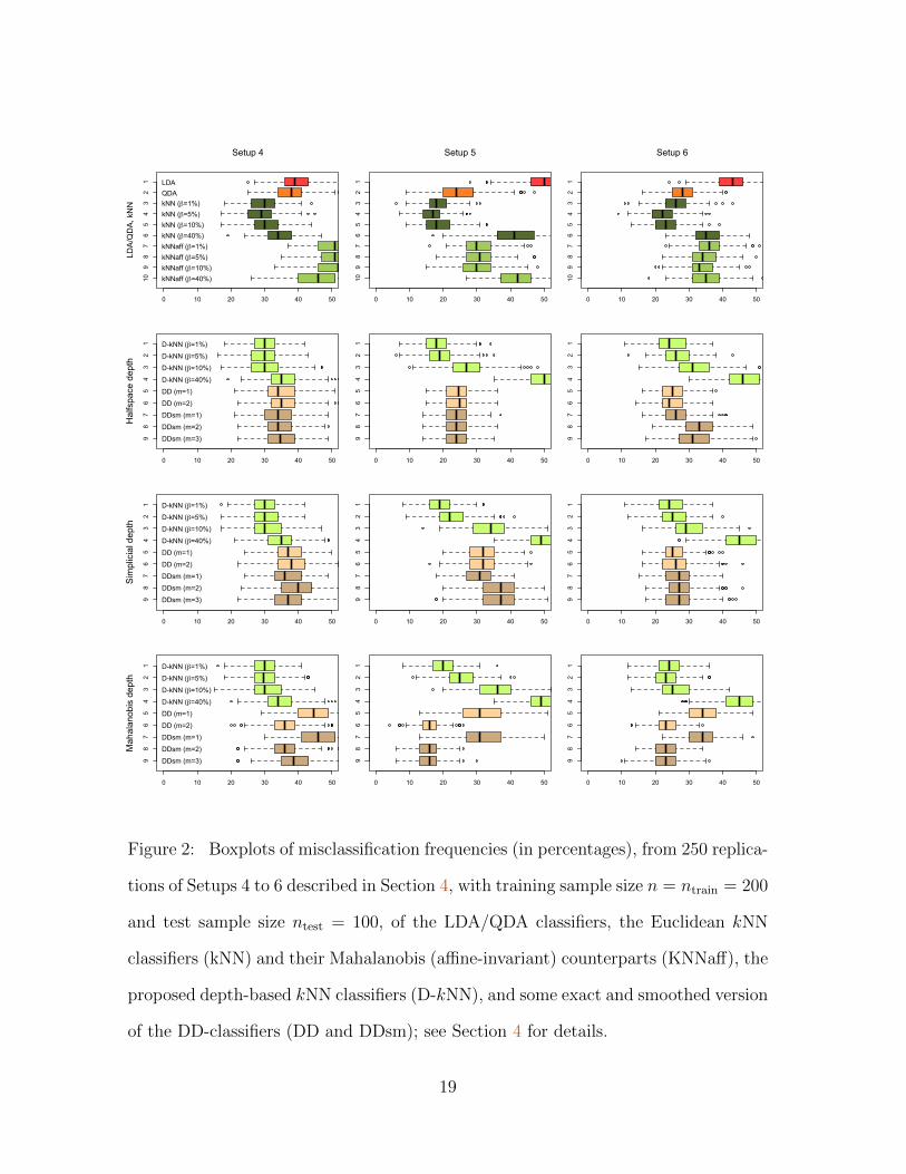
• The proposed depth-based kNN classifiers also compete well with DD-classifiers

both in elliptical and non-elliptical setups. Away from ellipticity (Setups 4

to 6), in particular, they perform at least as well—and sometimes outperform

(Setup 4)—DD-classifiers; a single exception is associated with the use of Ma-

halanobis depth in Setup 5, where the DD-classifiers based on m = 2, 3 per-

form better. Apparently, another advantage of depth-based kNN classifiers over

DD-classifiers is that their finite-sample performances depend much less on the

statistical depth function D used.

17

109

87

65

43

21

0 10 20 30 40 50

LDAQDAkNN (β=1%)kNN (β=5%)kNN (β=10%)kNN (β=40%)kNNaff (β=1%)kNNaff (β=5%)kNNaff (β=10%)kNNaff (β=40%)

LDA

/QD

A, k

NN

Setup 19

87

65

43

21

0 10 20 30 40 50

D-kNN (β=1%)

D-kNN (β=5%)

D-kNN (β=10%)

D-kNN (β=40%)

DD (m=1)

DD (m=2)

DDsm (m=1)

DDsm (m=2)

DDsm (m=3)

Hal

fspa

ce d

epth

98

76

54

32

1

0 10 20 30 40 50

D-kNN (β=1%)

D-kNN (β=5%)

D-kNN (β=10%)

D-kNN (β=40%)

DD (m=1)

DD (m=2)

DDsm (m=1)

DDsm (m=2)

DDsm (m=3)

Sim

plic

ial d

epth

98

76

54

32

1

0 10 20 30 40 50

D-kNN (β=1%)

D-kNN (β=5%)

D-kNN (β=10%)

D-kNN (β=40%)

DD (m=1)

DD (m=2)

DDsm (m=1)

DDsm (m=2)

DDsm (m=3)

Mah

alan

obis

dep

th

109

87

65

43

21

0 10 20 30 40 50

Setup 2

98

76

54

32

1

0 10 20 30 40 50

98

76

54

32

1

0 10 20 30 40 50

98

76

54

32

1

0 10 20 30 40 50

109

87

65

43

21

0 10 20 30 40 50

Setup 3

98

76

54

32

1

0 10 20 30 40 50

98

76

54

32

1

0 10 20 30 40 50

98

76

54

32

1

0 10 20 30 40 50

Figure 1: Boxplots of misclassification frequencies (in percentages), from 250 replica-

tions of Setups 1 to 3 described in Section 4, with training sample size n = ntrain = 200

and test sample size ntest = 100, of the LDA/QDA classifiers, the Euclidean kNN

classifiers (kNN) and their Mahalanobis (affine-invariant) counterparts (KNNaff), the

proposed depth-based kNN classifiers (D-kNN), and some exact and smoothed version

of the DD-classifiers (DD and DDsm); see Section 4 for details.

18

109

87

65

43

21

0 10 20 30 40 50

LDAQDAkNN (β=1%)kNN (β=5%)kNN (β=10%)kNN (β=40%)kNNaff (β=1%)kNNaff (β=5%)kNNaff (β=10%)kNNaff (β=40%)

LDA

/QD

A, k

NN

Setup 49

87

65

43

21

0 10 20 30 40 50

D-kNN (β=1%)

D-kNN (β=5%)

D-kNN (β=10%)

D-kNN (β=40%)

DD (m=1)

DD (m=2)

DDsm (m=1)

DDsm (m=2)

DDsm (m=3)

Hal

fspa

ce d

epth

98

76

54

32

1

0 10 20 30 40 50

D-kNN (β=1%)

D-kNN (β=5%)

D-kNN (β=10%)

D-kNN (β=40%)

DD (m=1)

DD (m=2)

DDsm (m=1)

DDsm (m=2)

DDsm (m=3)

Sim

plic

ial d

epth

98

76

54

32

1

0 10 20 30 40 50

D-kNN (β=1%)

D-kNN (β=5%)

D-kNN (β=10%)

D-kNN (β=40%)

DD (m=1)

DD (m=2)

DDsm (m=1)

DDsm (m=2)

DDsm (m=3)

Mah

alan

obis

dep

th

109

87

65

43

21

0 10 20 30 40 50

Setup 5

98

76

54

32

1

0 10 20 30 40 50

98

76

54

32

1

0 10 20 30 40 50

98

76

54

32

1

0 10 20 30 40 50

109

87

65

43

21

0 10 20 30 40 50

Setup 6

98

76

54

32

1

0 10 20 30 40 50

98

76

54

32

1

0 10 20 30 40 50

98

76

54

32

1

0 10 20 30 40 50

Figure 2: Boxplots of misclassification frequencies (in percentages), from 250 replica-

tions of Setups 4 to 6 described in Section 4, with training sample size n = ntrain = 200

and test sample size ntest = 100, of the LDA/QDA classifiers, the Euclidean kNN

classifiers (kNN) and their Mahalanobis (affine-invariant) counterparts (KNNaff), the

proposed depth-based kNN classifiers (D-kNN), and some exact and smoothed version

of the DD-classifiers (DD and DDsm); see Section 4 for details.

19

5 REAL-DATA EXAMPLES

In this section, we investigate the performances of our depth-based kNN classifiers on

two well known benchmark datasets. The first example is taken from Ripley (1996)

and can be found on the book’s website (http://www.stats.ox.ac.uk/pub/PRNN).

This data set involves well-specified training and test samples, and we therefore simply

report the test set misclassification rates of the different classifiers included in the

study. The second example, blood transfusion data, is available at http://archive.

ics.uci.edu/ml/index.html. Unlike the first data set, no clear partition into a

training sample and a test sample is provided here. As suggested in Li et al. (2012), we

randomly performed such a partition 100 times (see the details below) and computed

the average test set missclassification rates, together with standard deviations.

A brief description of each dataset is as follows:

Synthetic data was introduced and studied in Ripley (1996). The

dataset is made of observations from two populations, each of them being

actually a mixture of two bivariate normal distributions differing only in

location. As mentioned above, a partition into a training sample and a test

sample is provided: the training and test samples contain 250 and 1000

observations, respectively, and both samples are divided equally between

the two populations.

Transfusion data contains the information on 748 blood donors selected

from the blood donor database of the Blood Transfusion Service Center

in Hsin-Chu City, Taiwan. It was studied in Yeh et al. (2009). The

classification problem at hand is to know whether or not the donor gave

blood in March 2007. In this dataset, prior probabilities are not equal; out

of 748 donors, 178 gave blood in March 2007, when 570 did not. Following

20

Li et al. (2012), one out of two linearly correlated variables was removed

and three measurements were available for each donor: Recency (number

of months since the last donation), Frequency (total number of donations)

and Time (time since the first donation). The training set consists in 100

donors from the first class and 400 donors from the second, while the rest

is assigned to the test sample (therefore containing 248 individuals).

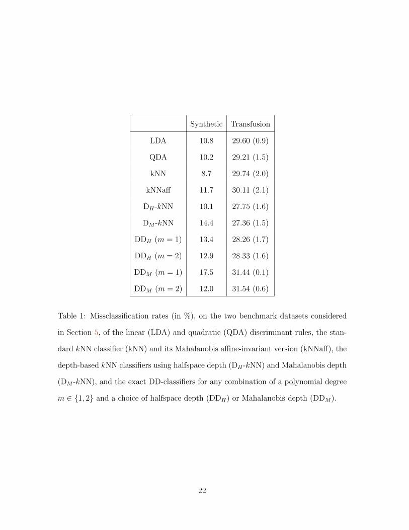
Table 1 reports the—exact (synthetic) or averaged (transfusion)—misclassification

rates of the following classifiers: the linear (LDA) and quadratic (QDA) discriminant

rules, the standard kNN classifier (kNN) and its Mahalanobis affine-invariant ver-

sion (kNNaff), the depth-based kNN classifiers using halfspace depth (DH-kNN) and

Mahalanobis depth (DM -kNN), and the exact DD-classifiers for any combination of

a polynomial order m ∈ {1, 2} and a statistical depth function among the two con-

sidered for depth-based kNN classifiers, namely the halfspace depth (DDH) and the

Mahalanobis depth (DDM)—smoothed DD-classifiers were excluded from this study,

as their performances, which can only be worse than those of exact versions, showed

much sensitivity to the smoothing parameter t; see Section 4. For all nearest-neighbor

classifiers, leave-one-out cross-validation was used to determine k.

The results from Table 1 indicate that depth-based kNN classifiers perform very

well in both examples. For synthetic data, the halfspace depth-based kNN classifier

(10.1%) is only dominated by the standard (Euclidian) kNN procedure (8.7%). The

latter, however, has to be discarded as it is dependent on scale and shape changes—in

line with this, note that the “kNN classifier” applied in Dutta and Ghosh (2012b)

is actually the kNNaff classifier (11.7%), as classification in that paper is performed

on standardized data. The Mahalanobis depth-based kNN classifiers (14.4%) does

not perform as well as its halfspace counterpart. For transfusion data, however, both

depth-based kNN classifiers dominate their competitors.

21

Synthetic Transfusion

LDA 10.8 29.60 (0.9)

QDA 10.2 29.21 (1.5)

kNN 8.7 29.74 (2.0)

kNNaff 11.7 30.11 (2.1)

DH-kNN 10.1 27.75 (1.6)

DM -kNN 14.4 27.36 (1.5)

DDH (m = 1) 13.4 28.26 (1.7)

DDH (m = 2) 12.9 28.33 (1.6)

DDM (m = 1) 17.5 31.44 (0.1)

DDM (m = 2) 12.0 31.54 (0.6)

Table 1: Missclassification rates (in %), on the two benchmark datasets considered

in Section 5, of the linear (LDA) and quadratic (QDA) discriminant rules, the stan-

dard kNN classifier (kNN) and its Mahalanobis affine-invariant version (kNNaff), the

depth-based kNN classifiers using halfspace depth (DH-kNN) and Mahalanobis depth

(DM -kNN), and the exact DD-classifiers for any combination of a polynomial degree

m ∈ {1, 2} and a choice of halfspace depth (DDH) or Mahalanobis depth (DDM).

22

6 FINAL COMMENTS

The depth-based neighborhoods we introduced are of interest in other inference prob-

lems as well. As an illustration, consider the regression problem where the conditional

mean function x 7→ m(x) = E[Y |X = x] is to be estimated on the basis of mutu-

ally independent copies (Xi, Yi), i = 1, . . . , n of a random vector (X, Y ) with values

in Rd × R, or the problem of estimating the common density f of i.i.d. random d-

vectors Xi, i = 1, . . . , n. The classical knNN estimators for these problems are

f (n)(x) =kn

nµd(Bβnx )

and m(n)(x) =n∑i=1

Wβn(n)i (x)Yi =

1

kn

n∑i=1

I[Xi ∈ Bβn

x

]Yi, (6.1)

where βn = kn/n, Bβx is the smallest Euclidean ball centered at x that contains

a proportion β of the Xi’s, and µd stands for the Lebesgue measure on Rd. Our

construction naturally leads to considering the depth-based knNN estimators f(n)D (x)

and m(n)D (x) obtained by replacing in (6.1) the Euclidean neighborhoods Bβn

x with

their depth-based counterparts Rβnx and kn =

∑ni=1 I

[Xi ∈ Bβn

x

]with K

βn(n)x =∑n

i=1 I[Xi ∈ Rβn

x

].

A thorough investigation of the properties of these depth-based procedures is of

course beyond the scope of the present paper. It is, however, extremely likely that

the excellent consistency properties obtained in the classification problem extend to

these nonparametric regression and density estimation setups. Now, recent works

in density estimation indicate that using non-spherical (actually, ellipsoidal) neigh-

borhoods may lead to better finite-sample properties; see, e.g., Chacon (2009) or

Chacon et al. (2011). In that respect, the depth-based kNN estimators above are

very promising since they involve non-spherical (and for most classical depth, even

non-ellipsoidal) neighborhoods whose shape is determined by the local geometry of

the sample. Note also that depth-based neighborhoods only require choosing a single

scalar bandwidth parameter (namely, kn), whereas general d-dimensional ellipsoidal

23

neighborhoods impose selecting d(d+ 1)/2 bandwidth parameters.

A APPENDIX

The main goal of this Appendix is to prove Theorem 3.1. We will need the following

lemmas.

Lemma A.1 Assume that the depth function D satisfies (P2), (P3), (Q1), and (Q2).

Let P be a probability measure that is symmetric about θθθ and admits a density that is

positive at θθθ and continuous in a neighborhood of θθθ. Then, (i) for all a > 0, there exists

α < α∗ = maxx∈Rd D(x, P ) such that Rα(P ) ⊂ Bθθθ(a) := {x ∈ Rd : ‖x− θθθ‖ ≤ a}; (ii)

for all α < α∗, there exists ξ > 0 such that Bθθθ(ξ) ⊂ Rα(P ).

Proof of Lemma A.1. (i) First note that the existence of α∗ follows from Property

(P2). Fix then δ > 0 such that x 7→ D(x, P ) is continuous over Bθθθ(δ); existence

of δ is guaranteed by Property (Q1). Continuity implies that x 7→ D(x, P ) reaches

a minimum in Bθθθ(δ), and Property (Q2) entails that this minimal value, αδ say, is

strictly smaller than α∗. Using Property (Q1) again, we obtain that, for each α ∈

[αδ, α∗],

rα : Sd−1 → R+

u 7→ sup{r ∈ R+ : θθθ + ru ∈ Rα(P )}

is a continuous function that converges pointwise to rα∗(u) ≡ 0 as α→ α∗. Since Sd−1

is compact, this convergence is actually uniform, i.e., supu∈Sd−1 |rα(u)| = o(1) as

α→ α∗. Part (i) of the result follows.

(ii) Property (Q2) implies that, for any α ∈ [αδ, α∗), the mapping rα takes values

in R+0 . Therefore there exists u0(α) ∈ Sd−1 such that rα(u) ≥ rα(u0(α)) = ξα > 0.

This implies that, for all α ∈ [αδ, α∗), we have Bθθθ(ξα) ⊂ Rα(P ), which proves the

24

result for these values of α. Nestedness of the Rα(P )’s, which follows from Prop-

erty (P3), then establishes the result for an arbitrary α < α∗. �

Lemma A.2 Assume that the depth function D satisfies (P2), (P3), and (Q1)-(Q3).

Let P be a probability measure that is symmetric about θθθ and admits a density that is

positive at θθθ and continuous in a neighborhood of θθθ. Let X1, . . . ,Xn be i.i.d. P and

denote by Xθθθ,(i) the ith depth-based nearest neighbor of θθθ. Let Kβn(n)θθθ be the number of

depth-based nearest neighbors in Rβnθθθ (P (n)), where βn = kn/n is based on a sequence kn

that is as in Theorem 3.1 and P (n) stands for the empirical distribution of X1, . . . ,Xn.

Then, for any a > 0, there exists n = n(a) such that∑K

βn(n)θθθ

i=1 I[‖Xθθθ,(i) − θθθ‖ > a] = 0

almost surely for all n ≥ n(a).

Note that, while Xθθθ,(i) may not be properly defined (because of ties), the quan-

tity∑K

βn(n)θθθ

i=1 I[‖Xθθθ,(i) − θθθ‖ > a] = 0 always is.

Proof of Lemma A.2. Fix a > 0. By Lemma A.1, there exists α < α∗ such that

Rα(P ) ⊂ Bθθθ(a). Fix then α and ε > 0 such that α < α−ε < α+ε < α∗. Theorem 4.1

in Zuo and Serfling (2000b) and the fact that P(n)θθθ → Pθθθ = P weakly as n → ∞

(where P(n)θθθ and Pθθθ are the θθθ-symmetrized versions of P (n) and P , respectively) then

entail that there exists an integer n0 such that

Rα+ε(P ) ⊂ Rα(P(n)θθθ ) ⊂ Rα−ε(P ) ⊂ Rα(P )

almost surely for all n ≥ n0. From Lemma A.1 again, there exists ξ > 0 such that

Bθθθ(ξ) ⊂ Rα+ε(P ). Hence, for any n ≥ n0, one has that

Bθθθ(ξ) ⊂ Rα(P(n)θθθ ) ⊂ Bθθθ(a)

almost surely.

Putting Nn =∑n

i=1 I[Xi ∈ Bθθθ(ξ)], the SLLN yields that Nn/n → P [Bθθθ(ξ)] =

P [Bθθθ(ξ)] > 0 as n → ∞, since X ∼ P admits a density that, from continuity, is

25

positive over a neighborhood of θθθ. Since kn = o(n) as n → ∞, this implies that, for

all n ≥ n0(≥ n0),n∑i=1

I[Xi ∈ Rα(P(n)θθθ )] ≥ Nn ≥ kn

almost surely. It follows that, for such values of n,

Rβnθθθ (P (n)) = Rβn(P

(n)θθθ ) ⊂ Rα(P

(n)θθθ ) ⊂ Bθθθ(a)

almost surely, with βn = kn/n. Therefore, maxi=1,...,K

βn(n)θθθ

‖Xθθθ,(i) − θθθ‖ ≤ a almost

surely for large n, which yields the result. �

Lemma A.3 For a “plug-in” classification rule m(n)(x) = I[η(n)(x) > 1/2] obtained

from a regression estimator η(n)(x) of η(x) = E[I[Y = 1] |X = x], one has that

P [m(n)(X) 6= Y ]−Lopt ≤ 2(E[(η(n)(X)−η(X))2]

)1/2, where Lopt = P [mBayes(X) 6= Y ]

is the probability of misclassification of the Bayes rule.

Proof of Lemma A.3. Corollary 6.1 in Devroye et al. (1996) states that

P [m(n)(X) 6= Y | Dn]− Lopt ≤ 2E[|η(n)(X)− η(X)| | Dn],

where Dn stands for the sigma-algebra associated with the training sample (Xi, Yi),

i = 1, . . . , n. Taking expectations in both sides of this inequality and applying

Jensen’s inequality readily yields the result. �

Proof of Theorem 3.1. From Bayes’ theorem, X admits the density x 7→ f(x) =

π0f0(x) + π1f1(x). Letting Supp+(f) = {x ∈ Rd : f(x) > 0} and writing C(fj) for

the collection of continuity points of fj, j = 0, 1, put N = Supp+(f)∩C(f0)∩C(f1).

Since, by assumption, Rd \C(fj) (j = 0, 1) has Lebesgue measure zero, we have that

P [X ∈ Rd \N ] ≤ P [X ∈ Rd \ Supp+(f)] +∑

j∈{0,1}

P [X ∈ Rd \ C(fj)]

=

∫Rd\Supp+(f)

f(x) dx = 0,

26

so that P [X ∈ N ] = 1. Note also that x 7→ η(x) = π1f1(x)/(π0f0(x) + π1f1(x)) is

continuous over N .

Fix x ∈ N and let Yx,(i) = Yj(x) with j(x) such that Xx,(i) = Xj(x). With this

notation, the estimator η(n)D (x) from Section 3.1 rewrites

η(n)D (x) =

n∑i=1

YiWβ(n)i (x) =

1

Kβ(n)x

Kβ(n)x∑i=1

Yx,(i).

Proceeding as in Biau et al. (2012), we therefore have that (writing for simplicity β

instead of βn in the rest of the proof)

T (n)(x) := E[(η(n)D (x)− η(x))2] ≤ 2T

(n)1 (x) + 2T

(n)2 (x),

with

T(n)1 (x) = E

[∣∣∣∣ 1

Kβ(n)x

Kβ(n)x∑i=1

(Yx,(i) − η(Xx,(i))

)∣∣∣∣2]and

T(n)2 (x) = E

[∣∣∣∣ 1

Kβ(n)x

Kβ(n)x∑i=1

(η(Xx,(i))− η(x)

)∣∣∣∣2].Writing D(n)

X for the sigma-algebra generated by Xi, i = 1, . . . , n, note that, condi-

tional onD(n)X , the Yx,(i)−η(Xx,(i))’s, i = 1, . . . , n, are zero mean mutually independent

random variables. Consequently,

T(n)1 (x) = E

[1

(Kβ(n)x )2

Kβ(n)x∑

i,j=1

E[(Yx,(i) − η(Xx,(i))

)(Yx,(j) − η(Xx,(j))

) ∣∣D(n)X

]]

= E

[1

(Kβ(n)x )2

Kβ(n)x∑i=1

E[(Yx,(i) − η(Xx,(i))

)2 ∣∣D(n)X

]]

≤ E

[4

Kβ(n)x

]≤ 4

kn= o(1),

27

as n→∞, where we used the fact that Kβ(n)x ≥ kn almost surely. As for T

(n)2 (x), the

Cauchy-Schwarz inequality yields (for an arbitrary a > 0)

T(n)2 (x) ≤ E

[1

Kβ(n)x

Kβ(n)x∑i=1

(η(Xx,(i))− η(x)

)2]

= E

[1

Kβ(n)x

Kβ(n)x∑i=1

(η(Xx,(i))− η(x)

)2I[‖Xx,(i) − x‖ ≤ a]

]

+E

[1

Kβ(n)x

Kβ(n)x∑i=1

(η(Xx,(i))− η(x)

)2I[‖Xx,(i) − x‖ > a]

]

≤ supy∈Bx(a)

|η(y)− η(x)|2 + 4E

[1

Kβ(n)x

Kβ(n)x∑i=1

I[‖Xx,(i) − x‖ > a]

]=: T2(x; a) + T

(n)2 (x; a).

Continuity of η at x implies that, for any ε > 0, one may choose a = a(ε) > 0 so

that T2(x; a(ε)) < ε. Since Lemma A.2 readily yields that T(n)2 (x; a(ε)) = 0 for large n,

we conclude that T(n)2 (x)—hence also T (n)(x)—is o(1). The Lebesgue dominated

convergence theorem then yields that E[(η(n)D (X)− η(X))2] is o(1). Therefore, using

the fact that P [m(n)D (X) 6= Y | Dn] ≥ Lopt almost surely and applying Lemma A.3, we

obtain

E[|P [m

(n)D (X) 6= Y | Dn]− Lopt|

]= E[P [m

(n)D (X) 6= Y | Dn]− Lopt]

= P [m(n)D (X) 6= Y ]− Lopt ≤ 2

(E[(η

(n)D (X)− η(X))2]

)1/2= o(1),

as n→∞, which establishes the result. �

Finally, we show that Properties (Q1)-(Q3) hold for several classical statistical

depth functions.

Theorem A.1 Properties (Q1)-(Q3) hold for (i) the halfspace depth and (ii) the

simplicial depth. (iii) If the location and scatter functionals µµµ(P ) and ΣΣΣ(P ) are such

28

that (a) µµµ(P ) = θθθ as soon as the probability measure P is symmetric about θθθ and such

that (b) the empirical versions µµµ(P (n)) and ΣΣΣ(P (n)) associated with an i.i.d. sample

X1, . . . ,Xn from P are strongly consistent for µµµ(P ) and ΣΣΣ(P ), then Properties (Q1)-

(Q3) also hold for the Mahalanobis depth.

Proof of Theorem A.1. (i) The continuity of D in Property (Q1) actually holds

under the only assumption that P admits a density with respect to the Lebesgue

measure; see Proposition 4 in Rousseeuw and Ruts (1999). Property (Q2) is a con-

sequence of Theorems 1 and 2 in Rousseeuw and Struyf (2004) and the fact that

the angular symmetry center is unique for absolutely continuous distributions; see

Serfling (2006). For halfspace depth, Property (Q3) follows from (6.2) and (6.6) in

Donoho and Gasko (1992).

(ii) The continuity of D in Property (Q1) actually holds under the only assumption

that P admits a density with respect to the Lebesgue measure; see Theorem 2 in Liu

(1990). Remark C in Liu (1990) shows that, for an angularly symmetric probability

measure (hence also for a centrally symmetric probability measure) admitting a den-

sity, the symmetry center is the unique point maximizing simplicial depth provided

that the density remains positive in a neighborhood of the symmetry center; Prop-

erty (Q2) trivially follows. Property (Q3) for simplicial depth is stated in Corollary 1

of Dumbgen (1992).

(iii) This is trivial. �

Finally, note that Properties (Q1)-(Q3) also hold for projection depth under very

mild assumptions on the univariate location and scale functionals used in the defini-

tion of projection depth; see Zuo (2003). �

29

References

Biau, G., Devroye, L., Dujmovic, V., and Krzyzak, A. (2012), “An Affine Invariant

k-Nearest Neighbor Regression Estimate,” arXiv:1201.0586v1, math.ST. 9, 14, 27

Chacon, J. E. (2009), “Data-driven Choice of the Smoothing Parametrization for

Kernel Density Estimators,” Canadian Journal of Statistics, 37, 249–265. 23

Chacon, J. E., Duong, T., and Wand, M. P. (2011), “Asymptotics for General Mul-

tivariate Kernel Density Derivative Estimators,” Statistica Sinica, 21, 807–840. 23

Cui, X., Lin, L., and Yang, G. (2008), “An Extended Projection Data Depth and

Its Applications to Discrimination,” Communications in Statistics - Theory and

Methods, 37, 2276–2290. 4

Dehon, C. and Croux, C. (2001), “Robust Linear Discriminant Analysis using S-

Estimators,” Canadian Journal of Statistics, 29, 473–492. 2

Devroye, L., Gyorfi, L., and Lugosi, G. (1996), A Probabilistic Theory of Pattern

Recognition (Stochastic Modelling and Applied Probability), New York: Springer.

13, 26

Donoho, D. L. and Gasko, M. (1992), “Breakdown Properties of Location Estimates

based on Halfspace Depth and Projected Outlyingness,” The Annals of Statistics,

20, 1803–1827. 29

Dumbgen, L. (1992), “Limit Theorems for the Simplicial Depth,” Statistics & Prob-

ability Letters, 14, 119–128. 29

— (1998), “On Tyler‘s M-Functional of Scatter in High Dimension,” Annals of the

Institute of Statistical Mathematics, 50, 471–491. 11

30

Dutta, S. and Ghosh, A. K. (2012a), “On Robust Classification using Projection

Depth,” Annals of the Institute of Statistical Mathematics, 64, 657–676. 3, 4

— (2012b), “On Classification Based on Lp Depth with an Adaptive Choice of p,”

Submitted. 3, 4, 21

Ghosh, A. K. and Chaudhuri, P. (2005a), “On Data Depth and Distribution-free

Discriminant Analysis using Separating Surfaces,” Bernoulli, 11, 1–27. 4

— (2005b), “On Maximum Depth and Related Classifiers,” Scandinavian Journal of

Statistics, 32, 327–350. 3, 11, 17

Hartikainen and Oja, H. (2006), “On some Parametric, Nonparametric and Semi-

parametric Discrimination Rules,” DIMACS Series in Discrete Mathematics and

Theoretical Computer Science, 72, 61–70. 3

He, X. and Fung, W. K. (2000), “High Breakdown Estimation for Multiple Popula-

tions with Applications to Discriminant Analysis,” Journal of Multivariate Analy-

sis, 72, 151–162. 2

Hettmansperger, T. P. and Randles, R. H. (2002), “A Practical Affine Equivariant

Multivariate Median,” Biometrika, 89, 851–860. 11

Hoberg, A. and Mosler, K. (2006), “Data Analysis and Classification with the Zonoid

Depth,” DIMACS Series in Discrete Mathematics and Theoretical Computer Sci-

ence, 72, 49–59. 11

Hubert, M. and Van der Veeken, S. (2010), “Robust Classification for Skewed Data,”

Advances in Data Analysis and Classification, 4, 239–254. 3

Jornsten, R. (2004), “Clustering and Classification Based on the L1 Data Depth,”

Journal of Multivariate Analysis, 90, 67–89. 4

31

Koshevoy, G. and Mosler, K. (1997), “Zonoid Trimming for Multivariate Distribu-

tions,” The Annals of Statistics, 25, 1998–2017. 7

Lange, T., Mosler, K., and Mozharovskyi, P. (2012), “Fast Nonparametric Classifi-

cation based on Data Depth,” Discussion Papers in Statistics and Econometrics

01/2012, University of Cologne. 4, 11

Li, J., Cuesta-Albertos, J., and Liu, R. Y. (2012), “DD-Classifier: Nonparametric

Classification Procedures based on DD-Plots,” Journal of the American Statistical

Association, to appear. 3, 11, 16, 17, 20, 21

Liu, R. Y. (1990), “On a Notion of Data Depth based on Random Simplices,” The

Annals of Statistics, 18, 405–414. 4, 7, 29

Liu, R. Y., Parelius, J. M., and Singh, K. (1999), “Multivariate Analysis by Data

Depth: Descriptive Statistics, Graphics and Inference,” The Annals of Statistics,

27, 783–840. 3, 11

Oja, H. and Paindaveine, D. (2005), “Optimal Signed-Rank Tests based on Hyper-

planes,” Journal of Statistical Planning and Inference, 135, 300–323. 9

Randles, R. H., Broffitt, J. D., Ramberg, J. S., and Hogg, R. V. (1978), “Generalized

Linear and Quadratic Discriminant Functions using Robust Estimates,” Journal of

the American Statistical Association, 73, 564–568. 2

Ripley, B. D. (1996), Pattern Recognition and Neural Networks, Cambridge: Cam-

bridge University Press. 20

Rousseeuw, P. J. and Ruts, I. (1999), “The Depth Function of a Population Distri-

bution,” Metrika, 49, 213–244. 29

32

Rousseeuw, P. J. and Struyf, A. (2004), “Characterizing Angular Symmetry and

Regression Symmetry,” Journal of Statistical Planning and Inference, 122, 161–

173. 8, 29

Serfling, R. J. (2006), “Multivariate Symmetry and Asymmetry,” Encyclopedia of

statistical sciences, 8, 5338–5345. 8, 29

Stone, C. J. (1977), “Consistent Nonparametric Regression,” The Annals of Statistics,

5, 595–620. 13

Tukey, J. W. (1975), “Mathematics and the Picturing of Data,” Proceedings of the

International Congress of Mathematicians, 2, 523–531. 4, 7

Tyler, D. E. (1987), “A Distribution-free M-Estimator of Multivariate Scatter,” The

Annals of Statistics, 15, 234–251. 11

Yeh, I. C., Yang, K. J., and Ting, T. M. (2009), “Knowledge Discovery on RFM Model

using Bernoulli Sequence,” Expert Systems with Applications, 36, 5866–5871. 20

Zakai, A. and Ritov, Y. (2009), “Consistency and Localizability,” Journal of Machine

Learning Research, 10, 827–856. 4

Zuo, Y. (2003), “Projection-based Depth Functions and Associated Medians,” The

Annals of Statistics, 31, 1460–1490. 29

Zuo, Y. and Serfling, R. (2000a), “General Notions of Statistical Depth Function,”

The Annals of Statistics, 28, 461–482. 6, 7

— (2000b), “Structural Properties and Convergence Results for Contours of Sample

Statistical Depth Functions,” The Annals of Statistics, 28, 483–499. 25

33