Embed Size (px)
Citation preview
Testing Option Pricing Models
David S. Bates
The Wharton School, University of Pennsylvaniaand the National Bureau of Economic Research
May 1995
The Wharton School, Suite 2300Philadelphia, PA 19104-6367

Testing Option Pricing Models
Abstract
This paper discusses the commonly used methods for testing option pricing models, including the
Black-Scholes, constant elasticity of variance, stochastic volatility, and jump-diffusion models. Since options
are derivative assets, the central empirical issue is whether the distributions implicit in option prices are
consistent with the time series properties of the underlying asset prices. Three relevant aspects of consistency
are discussed, corresponding to whether time series-based inferences and option prices agree with respect
to volatility, changes in volatility, and higher moments. The paper surveys the extensive empirical literature
on stock options, options on stock indexes and stock index futures, and options on currencies and currency
futures.
David S. BatesThe Wharton School, Suite 2300Philadelphia, PA 19104-6367
email: [email protected]

Contents
1. Introduction
2. Option pricing fundamentals2.1 Theoretical underpinnings: actual and "risk-neutral" distributions2.2 Terminology and notation2.3 Tests of no-arbitrage constraints on option prices
3. Time series-based tests of option pricing models3.1 Statistical methodologies3.2 The Black-Scholes model
3.2.1 Option pricing3.2.2 Tests of the Black-Scholes model3.2.3 Trading strategy tests of option market efficiency
3.3 The constant elasticity of variance model3.4 Stochastic volatility and ARCH models3.5 Jump-diffusion processes
4. Implicit parameter estimation4.1 Implicit volatility estimation4.2 Time series analyses of implicit volatilities4.3 Implicit volatilities as forecasts of future volatility4.4 Implicit volatility patterns: evidence for alternative distributional hypotheses
5. Implicit parameter tests of alternate distributional hypotheses5.1 CEV processes5.2 Stochastic volatility processes5.3 Jump-diffusions
6. Summary and Conclusions
1. Introduction
Since Black and Scholes published their seminal article on option pricing in 1973, there has
been an explosion of theoretical and empirical work on option pricing. While most papers maintained
Black and Scholes' assumption of geometric Brownian motion, the possibility of alternate
distributional hypotheses was soon raised. Cox and Ross (1976b) derived European option prices
under various alternatives, including the absolute diffusion, pure-jump, and square root constant
elasticity of variance models. Merton (1976) proposed a jump-diffusion model. Stochastic interest
rate extensions first appeared in Merton (1973), while models for pricing options under stochastic
volatility appeared in Hull and White (1987), Johnson and Shanno (1987), Scott (1987), and Wiggins
(1987). New models for pricing European options under alternate distributional hypotheses continue
to appear; for instance, Naik's (1993) regime-switching model and the implied binomial trees model
of Derman and Kani (1994) and Rubinstein (1994).
Since options are derivative assets, the central issue in empirical option pricing is whether
option prices are consistent with the time series properties of the underlying asset price. Three
aspects of consistency (or lack thereof) have been examined, corresponding to second moments,
changes in second moments, and higher-order moments. First, are option prices consistent with the
levels of conditional volatility in the underlying asset? Tests of this hypothesis include the early cross-
sectional tests of whether high-volatility stocks tend to have high-priced options, while more recent
papers have tested in a time series context whether the volatility inferred from option prices using the
Black-Scholes model is an unbiased and informationally efficient predictor of future volatility of the
underlying asset price. The extensive tests for arbitrage opportunities from dynamic option
replication strategies are also tests of the consistency between option prices and the underlying time
2
series, although it is not generally easy to identify which moments are inconsistent when substantial
profits are reported.
Second, the evidence from ARCH/GARCH time series estimation regarding persistent mean-
reverting volatility processes has raised the question whether the term structure of volatilities inferred
from options of different maturities is consistent with predictable changes in volatility. There has
been some work on this issue, although more recent papers have focussed on whether the term
structure of implicit volatilities predicts changes in implicit rather than actual volatilities. Finally,
there has been some examination of whether option prices are consistent with higher moments
(skewness, kurtosis) of the underlying conditional distribution. The focus here has largely been on
explaining the "volatility smile" evidence of leptokurtosis implicit in option prices. The pronounced
and persistent negative skewness implicit in U.S. stock index option prices since the 1987 stock
market crash is starting to attract attention.
The objective of this paper is to discuss empirical techniques employed in testing option
pricing models, and to summarize major conclusions from the empirical literature. The paper will
focus on three categories of financial options traded on centralized exchanges: stock options, options
on stock indexes and stock index futures, and options on currencies and currency futures. The
parallel literature on commodity options will largely be ignored; partly because of lack of familiarity,
and partly because of unique features in commodities markets (e.g., short-selling constraints in the
spot market that decouple spot and futures prices; harvest seasonals) that create unique difficulties
for pricing commodity options. The enormous literature on interest rate derivatives deserves its own
chapter; perhaps its own book.
The tests of consistency between options and time series are divided into two approaches:
those that estimate distributional parameters from time series data and examine the implications for
option prices, and those that estimate model-specific parameters implicit in option prices and test the
3
distributional predictions for the underlying time series. The two approaches employ fundamentally
different econometric techniques. The former approach can in principle draw upon methods of time
series-based statistical inference, although in practice few have done so. By contrast, implicit
parameter "estimation" lacks an associated statistical theory. A two-stage procedure is therefore
commonplace; the parameters inferred from option prices are assumed known with certainty and their
informational content is tested using time series data. Hybrid approaches are sorted largely on
whether their testable implications are with regard to option prices or the underlying asset price.
dS /S ' [µ & 8k ] dt % FS D&1 dW % k dq
dF ' µF(F) dt % <(F) dWF
dr ' µr (r ) dt % <r (r ) dWr
dS /S ' µ dt % FdW ,
dWF
ln(1% k ) - N [ ln(1% k ) & ½*2, *2 ]
4
(1)
(2)
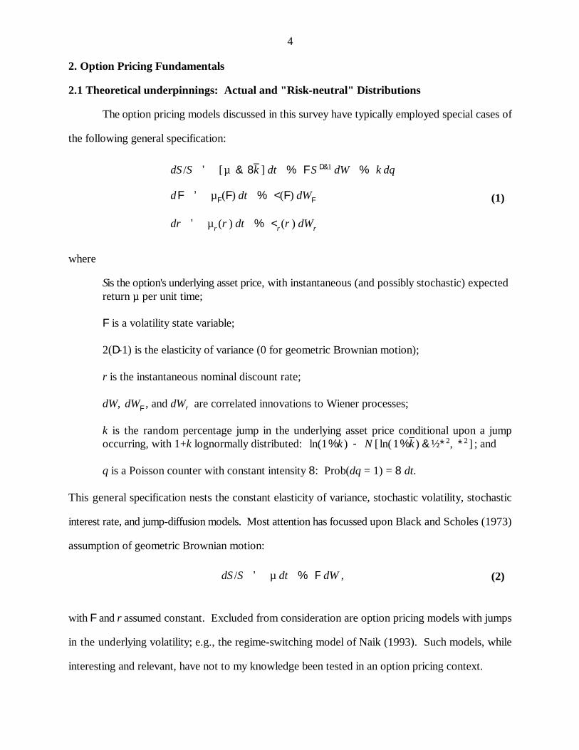
2. Option Pricing Fundamentals
2.1 Theoretical underpinnings: Actual and "Risk-neutral" Distributions
The option pricing models discussed in this survey have typically employed special cases of
the following general specification:
where
S is the option's underlying asset price, with instantaneous (and possibly stochastic) expectedreturn µ per unit time;
F is a volatility state variable;
2(D-1) is the elasticity of variance (0 for geometric Brownian motion);
r is the instantaneous nominal discount rate;
dW, , and dW are correlated innovations to Wiener processes;r
k is the random percentage jump in the underlying asset price conditional upon a jumpoccurring, with 1+k lognormally distributed: ; and
q is a Poisson counter with constant intensity 8: Prob(dq = 1) = 8 dt.
This general specification nests the constant elasticity of variance, stochastic volatility, stochastic
interest rate, and jump-diffusion models. Most attention has focussed upon Black and Scholes (1973)
assumption of geometric Brownian motion:
with F and r assumed constant. Excluded from consideration are option pricing models with jumps
in the underlying volatility; e.g., the regime-switching model of Naik (1993). Such models, while
interesting and relevant, have not to my knowledge been tested in an option pricing context.
c(S, T ; X ) ' E ( e&mT
0rt dt
max(ST & X, 0) .
dS /S ' [ r & 8( k( ] dt % FS D&1 dW ( % k ( dq (
dF ' [µF(F) dt % MF] % <(F) dW (F
dr ' [µr (r ) dt % M r ] % <r (r ) dW (r
MF ' Cov dF, dJw /Jw
M r ' Cov dr, dJw /Jw
8( ' 8E 1 % ) Jw /Jw
k( ' k %Cov (k , ) Jw /Jw )
E[1 % ) Jw /Jw ],
5
(3)
(4)
(5)
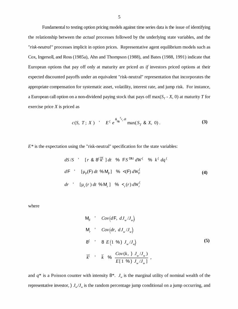
Fundamental to testing option pricing models against time series data is the issue of identifying
the relationship between the actual processes followed by the underlying state variables, and the
"risk-neutral" processes implicit in option prices. Representative agent equilibrium models such as
Cox, Ingersoll, and Ross (1985a), Ahn and Thompson (1988), and Bates (1988, 1991) indicate that
European options that pay off only at maturity are priced as if investors priced options at their
expected discounted payoffs under an equivalent "risk-neutral" representation that incorporates the
appropriate compensation for systematic asset, volatility, interest rate, and jump risk. For instance,
a European call option on a non-dividend paying stock that pays off max(S - X, 0) at maturity T forT
exercise price X is priced as
E* is the expectation using the "risk-neutral" specification for the state variables:
where
and q* is a Poisson counter with intensity 8*. J is the marginal utility of nominal wealth of thew
representative investor, )J /J is the random percentage jump conditional on a jump occurring, andw w
dS /S ' (r & r ( & 8( k( ) dt % FS D&1 dW ( % k ( dq ( .
dS /S ' r dt % FdW ( ,
6
(6)
(7)
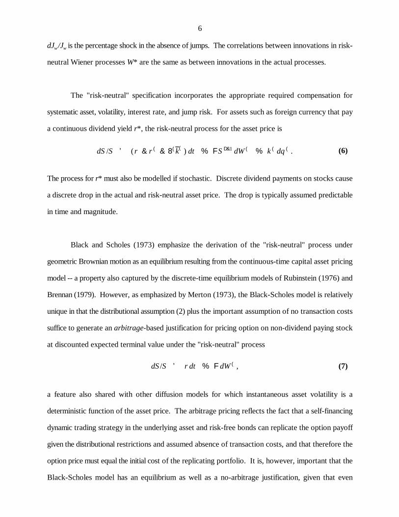
dJ /J is the percentage shock in the absence of jumps. The correlations between innovations in risk-w w
neutral Wiener processes W* are the same as between innovations in the actual processes.
The "risk-neutral" specification incorporates the appropriate required compensation for
systematic asset, volatility, interest rate, and jump risk. For assets such as foreign currency that pay
a continuous dividend yield r*, the risk-neutral process for the asset price is
The process for r* must also be modelled if stochastic. Discrete dividend payments on stocks cause
a discrete drop in the actual and risk-neutral asset price. The drop is typically assumed predictable
in time and magnitude.
Black and Scholes (1973) emphasize the derivation of the "risk-neutral" process under
geometric Brownian motion as an equilibrium resulting from the continuous-time capital asset pricing
model -- a property also captured by the discrete-time equilibrium models of Rubinstein (1976) and
Brennan (1979). However, as emphasized by Merton (1973), the Black-Scholes model is relatively
unique in that the distributional assumption (2) plus the important assumption of no transaction costs
suffice to generate an arbitrage-based justification for pricing option on non-dividend paying stock
at discounted expected terminal value under the "risk-neutral" process
a feature also shared with other diffusion models for which instantaneous asset volatility is a
deterministic function of the asset price. The arbitrage pricing reflects the fact that a self-financing
dynamic trading strategy in the underlying asset and risk-free bonds can replicate the option payoff
given the distributional restrictions and assumed absence of transaction costs, and that therefore the
option price must equal the initial cost of the replicating portfolio. It is, however, important that the
Black-Scholes model has an equilibrium as well as a no-arbitrage justification, given that even
Jw ' Uc (c) /P
MF
M r
µ(S ) ' $ ln(S /S )
7
For the consumption CAPM, the marginal utility of nominal wealth is related to the1
instantaneous marginal utility of consumption: , where c is real consumption and Pis the price level.
minuscule transaction costs vitiate the continuous-time no-arbitrage argument and preclude risk-free
exploitation of "arbitrage" opportunities.
Other models require some assessment of the appropriate pricing of systematic volatility risk,
interest rate risk, and/or jump risk. Standard approaches for pricing that risk have typically involved
either assuming the risk is nonsystematic and therefore has zero price ( = M = 0; 8* = 8, k* = k),r
or by imposing a tractable functional form on the risk premium (e.g., = >r) with extra (free)
parameters to be estimated from observed option prices. It has not been standard practice in the
empirical option pricing literature to price volatility risk or other sorts of risk using asset pricing
models such as the consumption-based capital asset pricing model. These risk premia can potentially1
introduce a wedge between the "risk-neutral" distribution inferred from option prices and the true
conditional distribution of the underlying asset price.
Even in the case of Black-Scholes, it is not possible to test the consistency of option prices
and time series without further restrictions on the relationship between the "actual" and "risk-neutral"
processes. For whereas the instantaneous conditional volatility F should theoretically be identical
across both processes, and therefore should be common to both the time series and option prices,
estimation of that parameter on the discretely sampled time series data typically available requires
restrictions on the functional form of µ. The issue is discussed in Grundy (1991) and Lo and Wang
(1995), who point out that strong mean reversion such as could introduce a
substantial disparity between the discrete-time sample volatility and the instantaneous conditional
volatility of log-differenced asset prices.
S S
F ' S e (r& r ( )T
F ' e rT [S & j t e &rt t Dt ]
8
Fama (1984) noted that the standard rejections of uncovered interest parity could be2
interpreted assuming rational expectations as evidence for a highly time-varying risk premium onforeign currencies. For surveys of the resulting literature, including alternate explanations, seeHodrick (1987), Froot and Thaler (1990) and Lewis (1995).
Tests of option pricing models therefore also rely to a certain extent on hypotheses regarding
the asset market equilibrium for the risk premium µ - r, or alternatively on empirically based
knowledge of the appropriate functional form for µ. In the above example, for instance, one might
argue in favor of a constant or slow-changing risk premium and against such strong mean reversion
as "implausible" either because of the magnitude of the speculative opportunities from buying when
S < and selling when S > or because of the empirical evidence regarding unit roots in asset
prices. Conditional upon a constant risk premium, of course, the probability limit of the volatility
estimate from log-differenced asset prices will be the volatility parameter F observed in option prices,
assuming Black-Scholes distributional assumptions.2
2.2 Terminology and Notation
The forward price F on the underlying asset is the price contracted now for future delivery.
For assets that pay a continuous dividend yield, such as foreign currencies, the forward and spot
prices are related by the "cost-of-carry" relationship , where r is the continuously
compounded yield from a discount bond of comparable maturity T, and r* is the continuous dividend
yield (continuously compounded foreign bond yield for foreign currency). For stock options with
known discrete dividend payments, the comparable relationship is ,
where dividends are discounted at the relevant discount bond yields r . Futures prices have zero costt
of carry.
A call option will be referred to as in-the-money (ITM), at-the-money (ATM), or out-of-the-
money (OTM) if the strike price is less than, approximately equal to, or greater than the forward
price on the underlying asset. For futures options, the futures price will be used instead of the
e &rT(F & X ) e &rT(X & F )
9
forward price. Similarly, put options will be in-, at-, or out-of-the-money if the strike is greater than,
approximately equal to, or less than the forward or futures price. This is standard terminology in
most of the literature, although some use the spot price/strike price relationship as a gauge of
moneyness. An ITM put corresponds in moneyness to an OTM call.
European call and put options that can be exercised only at maturity will be denoted c and p
respectively, while American options that can be exercised at any time prior to maturity will be
denoted C and P. The intrinsic value of a European option is the discounted difference between the
forward and strike prices: for calls, for puts. The intrinsic value of
American options is the value attainable upon immediate exercise: S - X for calls, X - S for puts.
Intrinsic value is important as an arbitrage-based lower bound on option prices. The time value of
an option is the difference between the option price and its intrinsic value.
The implicit volatility is the value for the annualized standard deviation of log-differenced
asset prices that equates the theoretical option pricing formula premised on geometric Brownian
motion with the observed option price. It is also commonly if ungrammatically called the "implied"
volatility. Implicit volatilities should in principle be computed using an American option pricing
formula when options are American, although this is not always done. Historical volatility is the
sample standard deviation for log-differenced asset prices over a fixed window preceding the option
transaction; e.g., 30 days.
2.3 Tests of no-arbitrage conditions
A necessary prerequisite for testing the consistency of time-series distributions and option
prices is that option prices satisfy certain basic no-arbitrage constraints. First, call and put option
prices relative to the synchronous underlying asset price cannot be below intrinsic value, while
American option prices cannot be below European prices. Second, American and European option
prices must be monotone and convex functions of the underlying strike price. Third, synchronous
10
European call and put prices of common strike price and maturity must satisfy put-call parity, while
synchronous American call and put prices must satisfy specific inequality constraints discussed in Stoll
and Whaley (1986).
Violation of these constraints either implies rejection of the fundamental economic hypothesis
of nonsatiation, or more plausibly indicates severe market synchronization or data recording
problems, bid-ask spreads, or transaction costs that have not been taken into account. Furthermore,
as discussed in Cox and Ross (1976a), these no-arbitrage constraints reflect extremely fundamental
properties of the risk-neutral distribution implicit in option prices. Monotonicity in European option
prices with respect to the strike price is equivalent to the risk-neutral distribution function being
nondecreasing, while nonconvexity is equivalent to risk-neutral probability densities being
nonnegative. If these no-arbitrage constraints are severely violated, there is no distributional
hypothesis consistent with observed option prices.
In general, there is reason to be skeptical of papers that report arbitrage violations based on
Wall Street Journal closing prices for options and for the underlying asset. Option prices are
extremely sensitive to the underlying asset price, and a lack of synchronization by even 15 minutes
can yield substantial yet spurious "arbitrage" opportunities. An early illustration is provided in Galai
(1979), who finds that most of the convexity violations observed for Chicago Board Options
Exchange (CBOE) stock option closing prices over April to October, 1973 (24 violations out of 1000
relevant observations) disappear when intradaily transactions data are used.
Nevertheless, studies that use more carefully synchronized transactions data have found that
substantial proportions of option prices violate lower bound constraints. Bhattacharya (1983)
examined CBOE American options on 58 stocks over August 24, 1976 to June 2, 1977 and found
1,120 violations (1.30%) out of 86,137 records violated the immediate-exercise lower bound, while
1,304 quotes out of a 54,735-record subset of the data (2.38%) violated the European intrinsic value
11
lower bound. Bhattacharya found very few violations net of estimated transaction costs, however.
Culumovic and Welsh (1994) found that the proportion of CBOE stock option lower bound
violations had declined by 1987-89, but was still substantial.
Evnine and Rudd (1985) examined the CBOE's American options on the S&P 100 index and
the American Stock Exchange's options on the Major Market Index using on-the-hour data over June
26 to August 30, 1984, during the first year the contracts were offered. They found 2.7% of the S&P
100 call quotations and 1.6% of the MMI call quotations violated intrinsic-value bounds, all during
turbulent market conditions in early August. The underlying indexes are not traded contracts, but
rather aggregate prices on the constituent stocks. Consequently, the apparent arbitrage opportunities
were not easily exploitable, and may reflect deviations of the reported index from its "true" value
because of stale prices.
Bodurtha and Courtadon (1986) examined Philadelphia Stock Exchange (PHLX) American
foreign currency options for five currencies during the market's first two years (February 28, 1983
to September 14, 1984), and found that .9% of the call transaction prices and 6.7% of the put prices
violated the immediate-exercise lower bounds computed from the Telerate spot quotations provided
by the exchange. Most violations disappeared when transaction costs were taken into account.
Ogden and Tucker (1987) examined 1986 pound, Deutschemark, and Swiss franc call and put options
time-stamped off the nearest preceding CME foreign currency futures prices. They found only .8%
violated intrinsic-value bounds, and that most violations were small. Bates (1995b) found roughly
1% of the PHLX Deutschemark call and put transaction prices over January 1984 to June 1991 mildly
violated intrinsic value bounds computed from futures prices. Hsieh and Manas-Anton (1988)
examined noon transactions for Deutschemark futures options during the first year of trading
(January 24 to October 10, 1984), and found 1.03% violations for calls and .61% for puts, all of
which were less than 4 price ticks.
12
Violations of intrinsic value constraints will only be observed for short-maturity, in-the-money
and deep-in-the-money options with little time value remaining -- a small proportion of the options
traded at any given time. The magnitude rather than the frequency of violations is consequently more
relevant. The fact that the violations are generally less than estimated transaction costs is reassuring,
and suggests that the violations may originate either in imperfect synchronization between the options
market and underlying asset market, or in bid-ask spreads. Further evidence of imperfect
synchronization is provided by Stephan and Whaley (1990), who found that stock options lagged
behind price changes in individual stocks by as much as 15 minutes in 1986, and by Fleming, Ostdiek,
and Whaley (1995), who found that S&P 100 stock index options anticipated subsequent changes in
the underlying stock index by about 5 minutes over January 1988 to March 1991. The violations
suggest measurement error in the observed option price/underlying asset price relationship even for
high-quality intradaily transactions data.
F̂2ML ) t '
1N jN
n'1ln(Sn /Sn&1 ) & ln(Sn /Sn&1)
2 ,
F̂2 ) t '1
N &1 jNn'1
ln(Sn /Sn&1 ) & ln(Sn /Sn&1)2 .
) t
13
(8)
(9)
3. Time Series-Based Tests of Option Pricing Models
3.1 Statistical Methodologies
If log-differenced asset prices were drawn from a stationary distribution, such as the Gaussian
distribution for log-differenced asset prices assumed by Black and Scholes (1973), then empirical tests
of the consistency of option prices with time series data would be relatively easy. The methods of
estimating the parameters of stationary distributions are well-established, and the resulting testable
implications for option prices are straightforward applications of statistical inference. For instance,
Lo (1986) proposed maximum likelihood parameter estimation, which given the invariance properties
yields maximum likelihood estimates of option prices conditional upon time series information.
Associated asymptotic confidence intervals for option prices can similarly be established, based upon
asymptotic unbiasedness and normality of estimated option prices. For the lognormal distribution,
the maximum likelihood estimator for data spaced at regular time intervals is of course
closely related to the usual unbiased estimator of variance
And since under geometric Brownian motion, N can be increased either by using more observations
or by sampling at higher frequency, arbitrarily tight confidence regions could in principle be
constructed for testing whether observed option prices are consistent with the underlying time series.
The only caveat is the distinction between the actual and "risk-neutral" mean of the distribution --
which, however, becomes decreasingly important as the data sampling frequency increases.
The approach of using high-frequency (e.g., intradaily) data for academic tests was initially
precluded by lack of data, and subsequently by the recognition of substantial intradaily market
microstructure effects such as bid-ask bounce that reduce the usefulness of that data. The appeal of
extending the length of the data sample was reduced by the recognition of time-varying volatility.
14
Tests of the Black-Scholes model have, therefore, typically involved some recognition that the model
is misspecified and that its underlying distributional assumption of constant-volatility geometric
Brownian motion with probability one is false.
Assorted alternate estimators premised on geometric Brownian motion have been proposed
for deriving time series-based predictions of appropriate option prices conditional on the use of a
relatively short data interval. Parkinson's (1980) high-low estimator exploited the information implicit
in the standard reporting of the day's high and low for a stock price, assuming intradaily geometric
Brownian motion. Garman and Klass (1980) discuss potential sources of bias in Parkinson's volatility
estimate, including noncontinuous recording (which biases reported highs and lows), bid-ask spreads,
and the (justified) concern that intradaily and overnight volatility can diverge. Butler and Schachter
(1986) noted that although sample variance was an unbiased estimator of the true variance, pricing
options off of sample variance yields biased option price estimates given the nonlinear transformation.
They consequently developed the small-sample minimum-variance unbiased estimator for Black-
Scholes option prices, by expanding option prices in a power series in F and using unbiased estimators
of the powers of F based upon the postulated normal distribution for log-differenced asset prices.
Butler and Schachter (1994), however, subsequently concluded that the small-sample bias induced
by using a 30-day sample variance was negligible for standard tests of option market efficiency,
especially relative to the noise in the small-sample volatility estimate. Bayesian methods have been
proposed that exploit prior information regarding the volatility (Boyle and Ananthanarayanan (1977))
or the cross-sectional distribution of volatilities across different stocks (Karolyi (1993)).
Finally, of course, the enormous literature on ARCH and GARCH models explicitly addresses
the issue of optimally estimating conditional variances when volatility is time-varying. The potential
value of these methods for option markets is examined by Engle, Kane, and Noh (1993), who conduct
a trading game in volatility-sensitive straddles (1 ATM call + 1 ATM put) between fictitious traders
who use alternative variance forecasting techniques. They conclude based on 1968-91 stock index

15
data that GARCH(1,1) traders would make substantial profits off moving-average "historical"
volatility traders, especially when trading very short-maturity straddles. Their results are substantially
affected by the 1987 stock market crash, however.
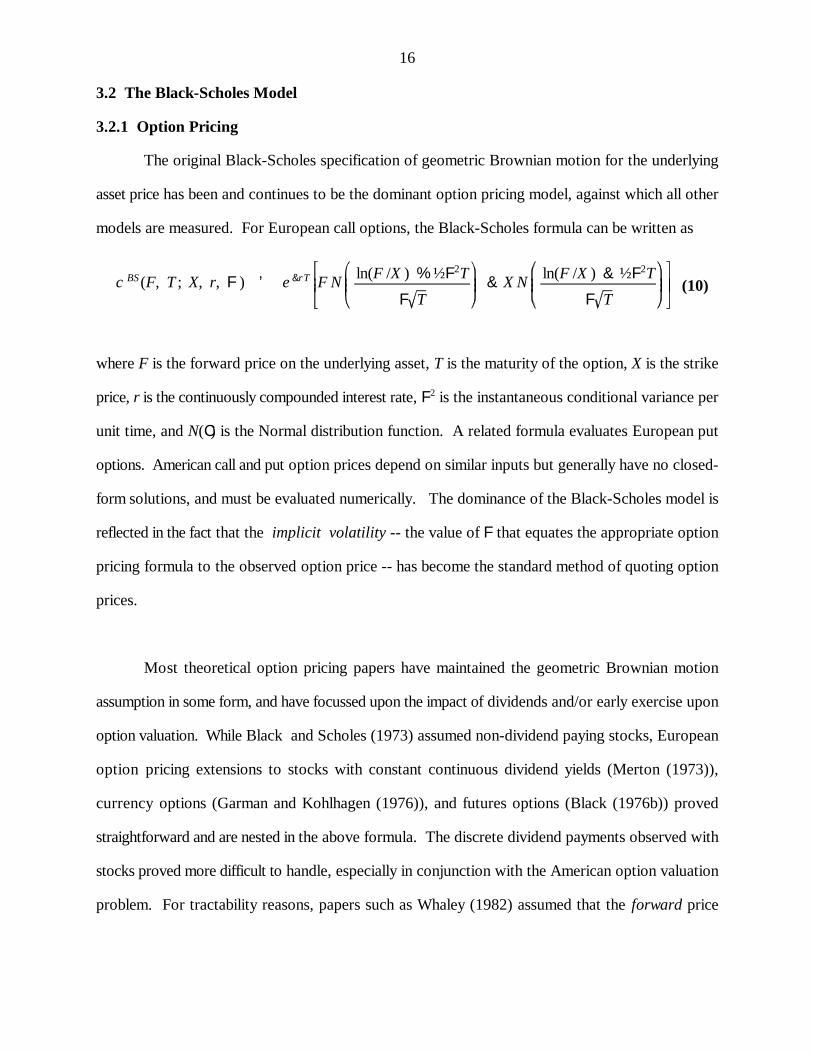
c BS(F, T ; X, r, F) ' e &rT F N ln(F /X ) % ½F2T
F T& X N ln(F /X ) & ½F2T
F T
16
(10)
3.2 The Black-Scholes Model
3.2.1 Option Pricing
The original Black-Scholes specification of geometric Brownian motion for the underlying
asset price has been and continues to be the dominant option pricing model, against which all other
models are measured. For European call options, the Black-Scholes formula can be written as
where F is the forward price on the underlying asset, T is the maturity of the option, X is the strike
price, r is the continuously compounded interest rate, F is the instantaneous conditional variance per2
unit time, and N(C) is the Normal distribution function. A related formula evaluates European put
options. American call and put option prices depend on similar inputs but generally have no closed-
form solutions, and must be evaluated numerically. The dominance of the Black-Scholes model is
reflected in the fact that the implicit volatility -- the value of F that equates the appropriate option
pricing formula to the observed option price -- has become the standard method of quoting option
prices.
Most theoretical option pricing papers have maintained the geometric Brownian motion
assumption in some form, and have focussed upon the impact of dividends and/or early exercise upon
option valuation. While Black and Scholes (1973) assumed non-dividend paying stocks, European
option pricing extensions to stocks with constant continuous dividend yields (Merton (1973)),
currency options (Garman and Kohlhagen (1976)), and futures options (Black (1976b)) proved
straightforward and are nested in the above formula. The discrete dividend payments observed with
stocks proved more difficult to handle, especially in conjunction with the American option valuation
problem. For tractability reasons, papers such as Whaley (1982) assumed that the forward price
F ' e rT [S & j t e &rt t Dt ]
17
Whaley's assumption that the stock price net of the present value of escrowed dividends3
follows geometric Brownian motion is equivalent to the assumption of geometric Brownian motionfor the forward price .
Examples include the MacMillan (1987) and Barone-Adesi and Whaley (1987) quadratic4
approximation for pricing American options on geometric Brownian motion. A good survey of theefficiency of alternative numerical methods is in Broadie and Detemple (1994).
See, e.g., Allegretto, Barone-Adesi, and Elliott (1994) and Broadie and Detemple (1994).5
rather than the cum-dividend stock price follows geometric Brownian motion. This yields a3
relatively simple formula for American call options when at most one dividend payment will be made,
and permits recombinant lattice techniques for numerically evaluating American options under
multiple dividend payments (Harvey and Whaley (1992a)).
Evaluating the early-exercise premium associated with American options has proved
formidable even under geometric Brownian motion. Computationally intensive numerical solutions
to the underlying partial differential equation are typically necessary, although good approximations
can be found in some cases. And although Kim (1990) and Carr, Jarrow, and Myneni (1992) have4
provided a clearer understanding of the "free-boundary" American option valuation problem, this has
only recently yielded more efficient American option valuation techniques. Concerns over the5
correct specification of boundary conditions and their impact on option prices continue to surface
(e.g., the "wild card" feature of S&P 100 index options discussed in Valerio (1993)), and are of
course fundamental to exotic option valuation. A major issue in the early empirical literature was
whether the use of European option pricing models with ad hoc corrections for the early-exercise
premium were responsible for reported option pricing errors; e.g., Whaley (1982), Sterk (1983), and
Geske and Roll (1984).
Many papers consequently concentrated upon cases in which American option prices are well
approximated by their European counterparts. For stock options, this involves examining only call
options on stocks with no or low dividend payments. American call (put) currency options are well
18
approximated by European currency option prices when the domestic interest rate is greater (less)
than the foreign interest rate (Shastri and Tandon (1986)).
3.2.2 Tests of the Black-Scholes Model
There have in fact been relatively few papers that estimate volatility from the past history of
log-differenced asset prices, and then test whether observed option prices are consistent with the
resulting predicted Black-Scholes option prices. One reason is that the equilibrium and no-arbitrage
foundations of the Black-Scholes model suggested proceeding directly to a "market efficiency" test
of the profits from dynamic option replication, as in Black and Scholes (1972). A second factor was
that early recognition of time-varying volatility made it more natural to reverse the test and examine
whether volatilities inferred from option prices did in fact correctly assess future asset volatility. The
former tests are discussed in the following section; the latter are surveyed in section 4.3 below.
Nevertheless, several papers used cross-sectional and event study methodologies to examine
the overall consistency of stock volatility with stock option prices. Black and Scholes (1972) and
Latané and Rendleman (1976) did find that high-volatility stocks tended to have high option prices
(equivalently, high implicit volatilities). However, Black and Scholes (1972) expressed concern that
the cross-sectional relationship was imperfect, with high-volatility stocks overpredicting and low-
volatility stocks underpredicting subsequent option prices. Black and Scholes examined over-the-
counter stock options during 1966-1969; but a similar relationship was found by Karolyi (1993) for
CBOE stock options over 1984-85. The possibility that this originates in an errors-in-variables
problem given noisy volatility estimates has not as yet been ruled out. Choi and Shastri (1989)
conclude that bid/ask-related biases in volatility estimation cannot explain the puzzle. Blomeyer and
Johnson (1988) found that Parkinson (1980) stock volatility estimates substantially underestimated
stock put option prices in 1978 even after adjusting for the early-exercise premium.
19
Event studies of predictable volatility changes have had mixed results. Patell and Wolfson
(1979) found that stock implicit volatilities increased up until earnings announcements and then
dropped substantially, which is consistent with predictable changes in uncertainty. Maloney and
Rogalski (1989) found that predictable end-of-year and January seasonal variations in common stock
volatility were in fact reflected in call option prices. By contrast, Sheikh (1989) found that
predictable increases in stock volatility following stock splits were not reflected in CBOE option
prices over 1976-1983 at the time the split was announced, but did influence option prices once the
split had occurred.
Cross-sectional evidence for currency and stock index options appears qualitatively consistent
with the risk on the underlying assets. Implicit volatilities reported in Lyons (1988) for Deutsche-
mark, pound and yen options over 1984-85 are comparable in magnitude to the underlying currency
volatility of 10-15% per annum. Options on S&P 500 futures typically had implicit volatilities of
15-20% over the three years prior to the stock market crash of 1987 (Bates (1991)), which is
comparable in magnitude to standard estimates of pre-crash stock market volatility.
That high-volatility assets typically have options with high implicit volatilities is reassuring,
especially given volatilities ranging from 5% on the Canadian dollar to 30%-40% on individual
stocks. The evidence of time-varying volatility from implicit volatilities and from ARCH/GARCH
models is sufficiently pronounced as to call into question the utility of more detailed time series/option
price comparisons premised upon constant volatility.
3.2.3 Trading Strategy Tests of Option Market Efficiency
Starting with Black and Scholes (1972), many have tested for dynamic arbitrage opportunities
that would indicate option mispricing. Such tests start with some assessment of volatility; Black and
Scholes used historical volatility from the preceding year, while others have used lagged daily implicit
volatilities. All options on a given day are evaluated using the Black-Scholes model (or an American
20
See Galai (1983) for a survey of early market efficiency tests.6
The elasticity of the Black-Scholes option price with regard to the underling asset price7
approaches infinity for options increasingly out-of-the-money, indicating a large impact from smallpercentage errors in the appropriate underlying asset price. George and Longstaff (1993) report thatbid-ask spreads on S&P 100 index options ranged from 2% to 20% of the option price in 1989.
option variant) and "overvalued" and "undervalued" options are identified. Appropriate option
positions are taken along with an offsetting hedge position in the underlying asset that is adjusted
daily using a "delta" based on the assessed volatility. Any resulting substantial and statistically
significant profits are interpreted as a rejection of the Black-Scholes model. Profits are often reported
net of the transaction costs associated with the daily alterations in the hedge positions. Since daily
hedging is typically imperfect and profits are risky, average profits are sometimes reported on a risk-
adjusted basis using Sharpe ratios or Jensen's alpha.6
The major problem with market efficiency tests is that they are extremely vulnerable to
selection bias. Imperfect synchronization with the underlying asset price and bid-ask spreads (on
options or on the underlying asset) can generate large percentage errors in option prices, especially
for low-priced out-of-the-money options. Consequently, even a carefully constructed ex ante test7
that only uses information from earlier periods doesn't guarantee that one can actually transact at the
option price/asset price combination identified as "overvalued" or "undervalued". An illustration of
this is Shastri and Tandon's (1987) observation with transactions data that delaying exploitation of
apparent opportunities by a single trade dramatically reduces average profits. The problem is of
course exacerbated in early studies that used badly synchronized closing price data.
A further statistical problem is that the distribution of profits from option trading strategies
is typically extremely skewed and leptokurtic. This is obviously true for unhedged options positions,
since buying options involves limited liability but unlimited potential profit. Merton (1976) points out
that this is also the case with delta-hedged positions and specification error. If the true process is a
21
jump-diffusion and options are priced correctly, profits from a correctly delta-hedged option position
follows a pure jump process: "excess" returns most of the time that are offset by substantial losses
on those occasions when the asset price jumps. And although skewed and leptokurtic profit
distributions may not pose problems asymptotically, whether t-statistic tests of no average excess
returns are reliable on the 1-3 year samples typically used has not been investigated.
A third problem with most "market efficiency" studies is that they give no information about
which options are mispriced. The typical approach pools options of different strike prices, maturities,
even options on different stocks. The "underpriced" options are purchased, the "overpriced" are sold,
and the overall profits are reported. Such tests do constitute a valid test of the hypothesis that all
options are priced according to the Black-Scholes model -- subject, of course, to the data and
statistical problems noted above. However, the omnibus rejections reported offer little guidance as
to why Black-Scholes is rejected, and which alternative distributional hypotheses would do better.
More detail is needed. Bad market volatility assessments, for instance, would affect all options, while
mispriced higher moments affect options of different strike prices differently. Greater detail would
also be useful in identifying whether the major apparent profit opportunities are in out-of-the-money
options, which are especially vulnerable to data problems. Studies such as Fleming (1994) that
restrict attention to at-the-money calls and puts appear more reliable and informative.
Many studies find excess profits that disappear after taking into account the transaction costs
from hedging the position in discrete time; e.g., Fleming (1994). While relevant from a practitioner's
viewpoint, these failures to reject Black-Scholes are not conclusive. Transaction costs vitiate the
arbitrage-based foundation of Black-Scholes, and it is not surprising that few arbitrage opportunities
net of transactions costs are found under daily hedging. The model does, however, have equilibrium
as well as no-arbitrage foundations. Testing these requires examining whether investing in or writing
"mispriced" options represents a speculative opportunity with excessively favorable return/risk
tradeoff. Unfortunately, testing option pricing models in an asset pricing context requires
dS /S ' µdt % FS D&1 dW
22
Black (1976a) noted that models of financial or operational leverage (i.e., that stockholders8
receive corporate income net of interest payments and other fixed costs) offered a partial explanationof the correlation. Black also noted, however, that leverage effects were insufficient to explain themagnitude of the price/volatility cross-effects.
(11)
substantially longer data bases than those employed hitherto -- especially given the skewed and
leptokurtic properties of option returns.
3.3 The Constant Elasticity of Variance Model
The constant elasticity of variance (CEV) option pricing model
first appeared in Cox and Ross (1976b) for the special cases D=½ and D=0. The more general model
subsequently appeared in MacBeth and Merville (1980), Emmanuel and MacBeth (1982), and Cox
and Rubinstein (1985). The model received attention for several reasons. First, the model is
grounded in the same no-arbitrage argument as the Black-Scholes model. Second, the model is
consistent with Black's (1976a) observation that volatility changes are negatively correlated with
stock returns -- a correlation subsequently if somewhat misleadingly referred to as "leverage effects."8
As such, there was initially some hope that the model could both explain and identify time-varying
volatility. Third, the model is potentially consistent with option pricing biases relative to the Black-
Scholes model. Fourth, the model is compatible with bankruptcy. Recent models of "implied
binomial trees" (Derman and Kani (1994); Rubinstein (1994)), which model instantaneous conditional
volatility as a flexible but deterministic function of the asset price and time, can be viewed as
generalizations of the CEV model.
Beckers (1980) estimated the CEV parameters for 47 stocks using daily data over 1972-1977,
and found return distributions were invariably less positively skewed than the lognormal (D<1) and
typically negatively skewed (D<0). He simulated option prices for the D=½ and D=0 cases, although
DÖ1
23
he did not explicitly test for compatibility with observed option prices. Gibbons and Jacklin (1988)
examined stock prices over a longer 1962-1985 data sample, and almost invariably estimated D
between 0 and 1. Melino and Turnbull (1991) estimated CEV processes for 5 currencies over 1979-
1986 with D constrained to discrete values between 0 and 1, inclusive, and typically rejected the
geometric Brownian motion hypothesis (D=1). Re-estimation over two subsamples of the 1983-1985
period for which they had currency option data revealed that all values of D considered were
essentially observationally equivalent both from time series data and with regard to predicted option
prices. All CEV models substantially underpredicted option prices during these first two years of
the Philadelphia currency option market.
In general, the CEV model seems unsuitable for stock index and currency options, and not
especially desirable for stock options. While bankruptcy is possible for stocks, it seems inconceivable
for stock indexes or currencies. Perhaps more important even for stock options, however, is that the
variance of asset returns is modelled as a deterministic and monotonic function of the underlying
nominal asset price. Given that asset prices have unit roots and typically non-zero drift, the CEV
model for implies that variance either approaches infinity or zero in the long run. The "implied
binomial tree" models suffer from a similar problem. Such models therefore require repeated
parameter recalibration, indicating fundamental misspecification.
3.4 Stochastic Volatility and ARCH Models
Given the substantial evidence summarized in Bollerslev, Chou and Kroner (1992) regarding
substantial and persistent changes in instantaneous volatility of asset returns, theorists in the 1970's
developed numerical methods for pricing options under stochastic volatility processes. The most
popular specification has been an Ornstein-Uhlenbeck process for the log of instantaneous conditional
volatility,
d (lnF) ' (" & $ lnF)dt % <dWF
dF2 ' (" & $F2 )dt % < F2dWF
2" < <2
24
(12)
(13)
with the log transformation enforcing nonnegativity constraints on volatility. The square root
stochastic variance process used inter alia by Cox, Ingersoll, and Ross (1985b) has also received
attention:
with a reflecting barrier at zero that is attainable when . Assorted assumptions are made
regarding the correlations between volatility shocks and asset and interest rate shocks. European
option pricing tractability (but not necessarily plausibility) is substantially increased for the former
process when shocks are uncorrelated. By contrast, Fourier inversion techniques proposed by Heston
(1993a) and Scott (1994) facilitate European option pricing for the latter process even when there
are non-zero volatility shock correlations with asset and interest rate shocks. There has been
relatively little empirical research thus far as to the correct specification; or indeed as to whether the
diffusion assumption is warranted. As discussed in section 2.1, assumptions regarding the form and
magnitude of the volatility risk premium are also necessary when pricing options off the risk-adjusted
versions of (12) or (13).
Estimation of stochastic volatility processes on discrete-time data has proved difficult, in two
dimensions. First, the fact that volatility is not directly observed implies that maximum likelihood
estimation of the parameters of the subordinated volatility process is at best computationally intensive
and often essentially impossible. Consequently, stochastic volatility parameter estimates have relied
either on time series analysis of volatility proxies such as short-horizon sample variances, or on
method of moments estimation using moments of the unconditional distribution of asset returns.
25
Scott (1987) proposed using a Kalman filter approach to infer the level of volatility -- an9
approach implemented by Harvey, Ruiz, and Shephard (1994). Kim and Shephard (1993) discuss theproblems posed by the failure of the asset return and volatility processes to satisfy the jointly Gaussianassumptions underlying the Kalman filter, and propose a remedy.
A caveat is that the implicit volatility is roughly the expected average risk-neutral volatility,10
which can deviate from the expected average volatility because of a volatility risk premium. Otherpotential problems with implicit volatilities are discussed in section 4.1 below.
Second, testing the implications of time series estimates for option prices under stochastic
volatility processes requires an assessment of the current level of instantaneous conditional volatility.
The filtration issue of identifying that volatility level given past information on asset returns is
difficult. Melino and Turnbull (1990), who used an extended Kalman filter, is one of the few papers
to directly tackle the issue in an option pricing context. Other option pricing "tests" of stochastic9
volatility models have either involved simulations of the implications for option prices of the
parameter estimates (e.g., Wiggins (1987)), or alternatively have inferred the instantaneous
conditional volatility from option prices conditional upon the parameter estimates. Examples of the
latter hybrid and two-stage approach include Scott (1987) for stock options, and Chesney and Scott
(1989) and Jorion (1995) for currency options.
There are three relevant tests of the stochastic volatility option pricing model relative to
Black-Scholes. First, variations over time in assessed volatility should outpredict future option prices
(equivalently, future implicit volatilities) relative to the Black-Scholes assumption of a constant
volatility inferred from log-differenced asset prices. Second, if volatility is mean-reverting then the
term structure of implicit volatilities across different option maturities should be upward (downward)
sloping whenever current volatility is below (above) its long-run average level. Third, the10
leptokurtic and possibly skewed asset return distributions implicit in stochastic volatility models
should be reflected in option price/implicit volatility patterns across different strike prices that deviate
from those generated by a lognormal distribution.
F̂2t T
26
None of the above papers employed the first test. This test is not possible under the hybrid
approaches, while Melino and Turnbull (1990) used the time-varying assessed volatility as an input
to both the stochastic volatility model and an ad hoc Black-Scholes model with continuously re-
adjusted F. Consequently, these papers effectively focussed on whether the estimated stochastict
volatility parameters can explain the cross-sectional patterns of option prices at different strike prices
and maturities relative to those generated by assuming a Gaussian distribution with variance for
maturity T.
Melino and Turnbull found that the stochastic volatility model did reduce the average and root
mean squared pricing errors on predicted Canadian dollar option prices over February 1983 to
January 1985 relative to the continuously readjusted and ad hoc Black-Scholes model, although the
volatility assessments do underpredict option prices on average. Most of the improvement appears
attributable to superior predictions of the term structure of implicit volatilities relative to the Black-
Scholes assumption of a flat term structure. Further substantial reconciliation of predicted and actual
option prices was achieved by judicious choice of the volatility risk premium -- a free parameter in
the model that substantially influences the term structure of implicit volatilities. Whether the sign and
magnitude reflect plausible compensation for volatility risk was not examined.
Melino and Turnbull (1990) used 47 moment conditions in conjunction with Hansen's (1982)
generalized method of moments (GMM) methodology, and estimated fairly tight standard errors on
their parameter estimates. It is difficult to have equal confidence in the parameter estimates and
option pricing predictions from other papers, given that the results appear sensitive to the limited
choice of moments. Wiggins (1987), for instance, estimated stochastic volatility parameters primarily
off of the moments of sample variances, and found the results quite sensitive to whether 2-, 4-, or 8-
day sample variances were used. Scott (1987) and Chesney and Scott (1989) used exactly identified
method of moments estimation based in part upon the unconditional second and fourth moments of
asset returns. The standard errors reported in Chesney and Scott (1989) indicate considerable
27
As discussed in Bollerslev, Chou and Kroner (1992), GARCH modelers have concluded that11
time-varying variance cannot explain all of the leptokurtosis in unconditional asset returns. CurrentGARCH models tend to assume fat-tailed shocks to the asset price. Ho, Perraudin and Sørensen(1993) estimate a stochastic volatility asset pricing model with jumps via GMM, and note thatinclusion of the jump component substantially affects parameter estimates.
imprecision. Furthermore, the use of fourth moments is vulnerable to specification error, given the
attribution to volatile volatility of any unconditional leptokurtosis originating in fat-tailed independent
shocks to the underlying asset price. Jorion (1995) used GMM estimation based on unconditional11
second moments of asset returns over different holding periods. The estimated standard errors are
enormous and the point estimates are implausible relative to the time series properties of implicit
volatilities.
The various autoregressive conditionally heteroskedastic (ARCH) models of time-varying
volatility are better designed for the twin problems of process and current volatility estimation from
discrete-time asset price data. These models converge in the continuous-time data sampling limit to
stochastic volatility models (Nelson (1990)), and provide consistent filtration-based estimates of
conditional variance even under misspecification (Nelson (1992)) provided the true volatility process
follows a diffusion. ARCH models consequently appear well suited for examining whether volatility
inferences from time series data are consistent with observed option prices. The downside is that it
can be difficult to price options off an estimated ARCH process. Conditional upon assumptions about
the appropriate volatility risk premium, European options can be priced via Monte Carlo simulations
of the risk-adjusted asset price/asset volatility processes. Most exchange-traded options are
American, however, for which Monte Carlo methods cannot readily be used.
Studies that have tested ARCH-based volatility assessments on option prices include Cao
(1992) for currency options, Myers and Hanson (1993) for commodity options, and Amin and Ng
(1993) for stock options. All three papers use ARCH-based volatility assessments as inputs to both
an ad hoc Black-Scholes option pricing model and the ARCH option pricing model. As with
F̂2t T
28
stochastic volatility papers, therefore, the focus is again on whether the ARCH models' predictions
of volatility mean reversion and higher-moment abnormalities fit option prices of different strike
prices and maturities better than assuming a Gaussian distribution with variance for maturity
T.
All three papers found some ability of ARCH-based option pricing models to correct Black-
Scholes pricing errors, albeit for different reasons. Cao (1992) found that Nelson's (1991) EGARCH
model outpredicted DM option prices in 1988 relative to a comparable-volatility Black-Scholes
model. The reasons for the superior performance are unclear. Myers and Hanson (1993) estimated
a rolling-regression GARCH(1,1)/Student's t process for soybean futures. They found that the major
gain for soybean futures option pricing prediction relative to Black's (1976b) geometric Brownian
motion model originated in the GARCH recognition of volatility mean reversion. Amin and Ng
(1993) examined the degree to which various ARCH models estimated on a 3-year moving window
that included the 1987 stock market crash could predict post-crash stock option prices over July 1988
to December 1989. All models overpredicted observed option prices, and had substantial moneyness-
and maturity-related biases. However, the substantially negatively skewed and leptokurtic models
such as EGARCH outpredicted the leptokurtic but essentially symmetric GARCH(1,1) model in
terms of overall option pricing mean absolute error, while the GARCH model outperformed a
comparable-volatility Black-Scholes forecast. Amin and Ng's option pricing improvements clearly
originate in superior modelling of the negatively skewed and leptokurtic distributions implicit in post-
crash stock option prices.
Overall, the tests of stochastic volatility and ARCH/GARCH option pricing models estimated
from time series data are still at an early stage, and far from conclusive. The simulated option trading
game in Engle, Kane and Noh (1993) suggests that GARCH(1,1) models are efficient volatility
estimators relative to moving-average estimates of sample volatility, but whether this translates into
superior predictions of option prices has not in fact been tested directly. Similarly, while some
29
calibrations of stochastic volatility models (e.g., Heston (1993a)) suggest that the higher-moment
implications of stochastic volatility shocks do not have a large impact on option prices, the time series
plausibility of the calibrations has not been definitively established. Indeed, the Amin and Ng (1993)
estimates offer evidence to the contrary, although their modelling assumption that the 1987 stock
market crash was just a bad draw from a conditionally normal distribution is questionable.
For currency options, the primary testable implications of time-varying volatility models
appears to lie in whether the conditional volatility is comparable to volatilities inferred from option
prices. Whether the typical estimates of a mean-reverting volatility process are consistent with the
term structure of implicit volatilities can also be tested. For stock and stock index options, an outlier
of the magnitude of October 19-20, 1987 poses possibly insurmountable problems for estimating
stochastic volatility-based option prices from time series data on the underlying asset price.
30
3.5 Jump-Diffusion Processes
Merton (1976) suggested that distributions with fatter tails than the lognormal might explain
the tendency for deep-in-the-money, deep-out-of-the money, and short-maturity options to sell for
more than their Black-Scholes value, and the tendency of near-the-money and longer-maturity options
to sell for less. Merton priced options on jump-diffusion processes under the assumption of
diversifiable jump risk and independent lognormally distributed jumps. Subsequent work by Jones
(1984), Naik and Lee (1990), and Bates (1991) indicates that Merton's model with modified
parameters is still relevant even under nondiversifiable jump risk. Others have proposed alternate
option pricing models under fat-tailed shocks: McCulloch's (1987) stable Paretian model, Madan and
Seneta's (1990) variance-gamma model, and Heston's (1993b) gamma process.
As of current writing, only Merton's (1976) model has been used in time series-based tests
of option pricing models. Apart from early work by Press (1967) using the method of cumulants,
most papers have used maximum likelihood estimation along with a truncation of the infinite series
representation of the likelihood function. Ball and Torous (1985) estimated jump-diffusion processes
with mean-zero jumps for 30 NYSE stocks, using daily cum-dividend returns over January 1, 1981
to December 31, 1982. They generated theoretical Merton and Black-Scholes European option
prices with strike prices and maturities matching those observed for CBOE and AMEX American call
options on these stocks on January 3, 1983. They concluded that the Merton and Black-Scholes
option prices were essentially indistinguishable for the estimated parameters, except for out-of-the-
money January options with less than a month to maturity. Trautmann and Beinert (1994) estimated
high-frequency (0.3 - 2.2 jumps/day) low-amplitude jumps for 14 German stocks based on daily data
over 1981-85 and 1986-1990, and found that the resulting option prices are virtually identical to
those generated from a comparable-volatility no-jump specification.
Jorion (1988) similarly estimated jump-diffusion parameters for the $/DM exchange rate and
the CRSP value-weighted stock index using weekly and monthly data over January 1974 to
31
The problem of maximum likelihood estimation given a multiple infinite summation series12
representation for transition densities can be finessed by instead using Fourier inversion of thecharacteristic function to evaluate those densities.
December 1985, both with and without an ARCH(1) specification for non-jump conditional volatility.
His estimate for $/DM of 1.32 jumps per week with mean jump size essentially 0 and standard
deviation of 1.17% induces substantial percentage pricing biases (relative to Black-Scholes values)
in OTM options of less than 1-month maturity, but has negligible impact on longer maturities. Jorion
noted that the biases are partially but not fully consistent with biases in DM options over 1983-85
reported by Bodurtha and Courtadon (1987), but did not explicitly test that consistency. For the
CRSP stock index, Jorion estimated .17 jumps/week with jump mean of 0 and standard deviation of
3.34%. Simulations again indicate the largest pricing impact for options of less than 1 month
maturity, but also some substantial impact on longer maturities. Whether the estimated pricing biases
are consistent with those observed in stock index options was not discussed.
Jump-diffusion parameter estimates from daily or weekly data typically find high-frequency
low-amplitude jump components of relevance only to options with very short maturities. It seems
likely that such estimates are picking up lumpy information flows associated with macroeconomic or
firm-specific data announcements, as discussed in Ederington and Lee (1993). Whether there is also
a low-frequency large-amplitude component such as would be more consistent with 1-6 month option
pricing anomalies is difficult to ascertain. It is hard to identify low-frequency jumps on the short data
intervals (less than 10 years) typically employed, so parameter estimates for a single jump process
naturally gravitate towards the identifiable high-frequency phenomena. A possible solution would
be to expand the data set and have two or more independent jump processes, but I know of no paper
that has implemented this approach on financial data. 12
4. Implicit Parameter Estimation
It has been common when examining option pricing models to infer some or all of the
distributional parameters from option prices conditional upon the postulated model, rather than
32
estimating parameters from time series data on the underlying asset price. The interest in implicit
parameters reflects the fact that options are forward-looking assets, with prices sensitive to
distributional moments such as future volatility. Much of the academic interest in options has
reflected the potential ability of option prices to offer insights into market expectations of future
distributions that are more difficult to infer from time series analysis.
A major problem with implicit parameter estimation is that we have no associated statistical
theory. Option pricing models are premised upon the underlying parameters and
distributional structure being known with certainty, so that implicit parameters should in principle be
a matter of inversion rather than estimation. An obvious overidentification problem arises when there
are N parameters and N+K option prices. And although measurement error in option prices offers
one justification for aggregating information from different option prices, the alternative hypothesis
that inconsistencies across options may reflect specification error must constantly be kept in mind.
Tests involving implicit parameters are inherently two-stage: information (e.g., implicit volatilities)
is inferred from option prices under some aggregation scheme, and is treated as the null hypothesis
to be tested using time series data.
4.1 Implicit Volatility Estimation
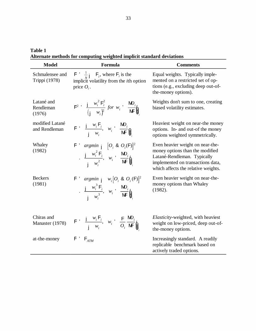
Within the Black-Scholes paradigm, a single option quote suffices to identify the implicit
parameter F; see (10). Since synchronous option prices of different strike prices and maturities yield
different F's, assorted schemes have been proposed for aggregating the information from different
options into a single volatility assessment. The major methods are summarized in Table 1. Most
involve weighting schemes that assign equal weight to in- and out-of-the-money options,
F̂ ' 1
N j Fi
F̂2 ' j w 2i F
2i
j wi2
for wi ' /000MOi
MF Fi
F̂ ' j wi Fij wi
, /000wi 'MOi
MF Fi
F̂ ' argmin j Oi & Oi(F) 2
. j w 2i Fi
j w 2i
, /000wi 'MOi
MF Fi
F̂ ' argmin j wi Oi & Oi (F) 2
. j w 3i Fi
j w 3i
, /000wi 'MOi
MF Fi
F̂ 'j wi Fij wi
, /000wi 'FOi
MOi
MFFi
F̂ ' FATM
33
Table 1Alternate methods for computing weighted implicit standard deviations
Model Formula Comments
Schmalensee and , where F is the Equal weights. Typically imple-Trippi (1978) mented on a restricted set of op-
i
implicit volatility from the ith optionprice O .i tions (e.g., excluding deep out-of-
the-money options).
Latané and Weights don't sum to one, creatingRendleman biased volatility estimates.(1976)
modified Latané Heaviest weight on near-the moneyand Rendleman options. In- and out-of the money
options weighted symmetrically.
Whaley Even heavier weight on near-the-(1982) money options than the modified
Latané-Rendleman. Typicallyimplemented on transactions data,which affects the relative weights.
Beckers Even heavier weight on near-the-(1981) money options than Whaley
(1982).
Chiras and Elasticity-weighted, with heaviestManaster (1978) weight on low-priced, deep out-of-
the-money options.
at-the-money Increasingly standard. A readilyreplicable benchmark based onactively traded options.
MO /MF
34
See Day and Lewis (1988) for a comparison of the Chiras and Manaster (1978) and Whaley13
(1982) weighting schemes.
See George and Longstaff (1993) for evidence of irregular bid-ask spreads across different14
strike prices and maturities.
and most give heavier weight to near-the-money options. The exception is Chiras and Manaster
(1978), where a focus on percentage pricing errors results in the heaviest weight falling on the
deepest out-of-the-money call and put options. A further issue is the choice between point-in-time13
option prices (e.g., closing or settlement prices) and pooled transactions data over some interval (e.g.,
daily). Since near-the-money call and put options are typically most heavily traded on centralized
exchanges, and trading activity differs for in- and out-of-the-money options, the use of transactions
data further affects the relative weights. Given time-varying volatility, it is desirable to construct
maturity-specific implicit volatilities from options of a common maturity. Some studies, however,
pool across maturities.
Underlying the alternate weighting schemes is an implicit presumption of independent
measurement error in option prices. Given nonconstant "vega" across different strike prices,
this can translate into substantial noise in implicit volatilities, especially from deep in- and out-of-the-
money options. There has, however, been little explicit scrutiny of the nature of this presumed
measurement error across strike prices and maturities, and what it implies for optimal weights. For
instance, while Whaley's (1982) methodology is consistent with homoskedastic white noise in option
prices, there has been little verification of that underlying assumption. Plausible explanations of
measurement error include bid-ask spreads or imperfect synchronization with the underlying asset
price -- both of which suggest heteroskedastic option pricing errors that are related to moneyness and
maturity. Engle and Mustafa (1992) and Bates (1995b) propose a nonlinear generalized least14
squares methodology that allows the appropriate weights to be determined endogenously by the data.
c (F, T ; X, r , FF ) ' e &r T F Nln(F /X ) % ½F2
FT
FF T& X N
ln(F /X ) & ½F2FT
FF T
35
If the true parameters are F=20% and r=10%, erroneously using a 9.7% interest rate yields15
a 20.22% implicit volatility from a 90-day at-the-money option, with comparable effects at longermaturities. Hammer notes the effects differ with strike price. The implicit volatilities from 10% in-and out-of-the-money options would be 20.11% and 20.71%, respectively.
(14)
Apart from measurement error in option prices or in the underlying asset prices, there are
other potential sources of bias when inferring the volatility parameter from observed option prices.
First is the issue of selecting the appropriate short-term interest rate to put into the Black-Scholes
formula, whether from Treasury bills, commercial paper, or Eurodollars. Most academic studies use
Treasury bill yields, but this is less common among practitioners. Furthermore, most empirical tests
use the same daily interest rate for evaluating all options on a given day, even when intradaily
transactions data are used. Simulations by Hammer (1989) indicate a fairly small impact on at-the-
money implicit volatilities from using the wrong interest rate. Some have attempted to infer which15
is the appropriate interest rate using pairs of options; e.g., Brenner and Galai (1986) and French and
Martin (1987). Results are somewhat inconclusive, but suggest that the Treasury bill rate is probably
too low.
Second, the common practice of using a new interest rate every day suggests that a stochastic
interest rate model would be more appropriate. However, the fact that interest rates are stochastic
does not appear to be a major concern when inferring volatilities from short-term European option
prices. If the instantaneous nominal domestic interest rate follows an Ornstein-Uhlenbeck process,
then a Black-Scholes formula still applies:
F2F
36
Stochastic interest rate and bond price models that generate option prices of this form are16
in Merton (1973), Grabbe (1983), Rabinovitch (1989), Hilliard, Madura, and Tucker (1991), andAmin and Jarrow (1991). For foreign currency options it is necessary to impose comparabledistributions on foreign interest rates or foreign bond prices.
Scott (1994) develops stock option pricing formulas applicable in the Cox et al (1985b)17
environment.
where r is the continuously-compounded yield from a discount bond of comparable maturity T and
, the average conditional variance of the forward price over the lifetime of the option, is a
deterministic function of time under this interest rate process. This specification is not valid for16
other interest rate processes (e.g., the square root interest rate process of Cox, Ingersoll, and Ross
(1985b)) , nor of course is it valid for American options. Nevertheless, the model suggests that the17
standard practice of using the yield from a contemporaneous and comparable-maturity Treasury bill
captures the major impact of changing interest rates over time. Furthermore, the fact that interest
rates are stochastic and possibly correlated with the underlying asset price is largely captured by the
recognition that it is the volatility of the forward price rather than the spot price that is implicit in
option prices. There is little difference between the two for options maturing in less than a year,
although the difference can matter at longer maturities. Ramaswamy and Sundaresan (1985) examine
American futures option pricing under square root stochastic interest rate processes, and conclude
that the term structure of interest rates significantly affects short-term American option prices but the
fact that interest rates are stochastic does not.
Many have pointed out the internal inconsistency involved in re-estimating implicit conditional
volatilities daily using a model premised on constant volatility. The impact of the specification error
can be assessed using the observation by Hull and White (1987) and Scott (1987) that if volatility
evolves independently of the asset price, then the true European option price is the expected value
c BS ' e &r TF [2N (½F T ) & 1]
c ' m4
V ' 0c BS ( V ) f ( (V ) dV ' E (
t c BS( V ) .
c BS (F̂) ' c . c BS E (t V %
12M 2c BS
(M F2)2/0000F2 ' E (
t VVar (t (V )
F̂2
E (t V
. 1 &18
Var (t (V )
[E (t (V )]2
.
F̂2
c BS . e &r TF F T /2B
37
It is important to note that (15) is an expectation over average variance -- not average18
volatility. A confusion between the two has led some to erroneously conclude that at-the-moneyimplicit volatilities should be unbiased estimates of future volatility.
For at-the-money options, F = X and (10) can be written as19
. Expanding N(C) in a second-order Taylor series around 0 yieldsthe approximation.
(15)
(16)
(17)
under the risk-neutral distribution of the Black-Scholes option price conditional on the realized
average variance over the option's maturity:18
A similar relationship holds for Merton's (1976) jump-diffusion model with mean-zero jumps. Using
a Taylor series expansion,
which indicates that the implicit variance inferred using the Black-Scholes formula will be biased
upward (downward) relative to risk-neutral expected average variance in regions where the Black-
Scholes formula is predominantly convex (concave) in F . For at-the-money options, the second-2
order Taylor approximation can be used in conjunction with (16) to further19
clarify the relationship between implicit and risk-neutral expected average variance:
There are three caveats. First, the expected average variance under the risk-neutral measure
will differ from the true expected average variance if there is a volatility risk premium. Second, (15)
is invalid for options on stocks and stock indexes, given the strong negative correlations observed
38
between price and volatility shocks for these assets. Equation (15) is also invalid for Merton's jump-
diffusion model when jumps have non-zero mean -- another skewed distribution. Consequently, the
reliability of implicit volatilities premised on lognormality when the actual distribution is substantially
skewed has not been established. Third, (15) - (17) are only valid for European options.
Nevertheless, at-the-money implicit volatilities appear relatively robust estimates of future
volatility under the alternative distributional hypotheses typically considered, although it is certainly
possible to identify parameter values for which this is not the case. Estimates of the volatility of
volatility from the time series properties of implicit volatilities suggest that the Jensen's inequality bias
in implicit volatilities is typically less than .5% for 1- to 12-month at-the-money options. The
difference between actual and "risk-neutral" expected average variance is unknown, but is not likely
to be a major factor for short-maturity options. Finally, estimates of implicit parameters under
moderately skewed jump-diffusion processes in Bates (1991, 1995a) almost invariably yield implicit
volatilities that diverge by less than 1% from the volatilities inferred using an American option variant
of the Black-Scholes model.
4.2 Time Series Properties of Implicit Volatilities
There has been substantial interest in the time series properties of implicit volatilities. First,
since implicit volatilities are a direct proxy for option prices, such analyses offer direct and readily
interpretable insights into the evolution of option markets. Second, if implicit volatilities are good
proxies for expected future volatility of the underlying asset price, then further insights into volatility
EtV '"$
[1 & w(T& t )] % w (T& t )Vt
Et V Vt
w(T& t ) ' [1 & e &$(T& t )] / [$(T& t )]Vt Et V
F̂2t . E (
t V . Et V
39
"Consistent" does not, of course, mean identical. The two processes can differ because of20
a volatility risk premium.
For (13), there is a parameter-dependent linear mapping between the expected average21
variance and the instantaneous conditional variance :
where , and T - t is the option maturity at time t. This can beused to estimate the parameters " and $ of the process given data. The procedure does ofcourse involve assuming . A bias correction based on (17) can improve the firstapproximation.
processes can be obtained. Poterba and Summers (1986), for instance, use implicit volatility
dynamics to assess how much stock prices should respond to volatility shocks..
Several procedural issues arise with regard to time series analysis of implicit volatilities. First,
the volatilities should ideally be inferred using a stochastic volatility option pricing model that is
consistent with the model fitted to the resulting time series of implicit volatilities. As discussed20
above, however, implicit variances as measures of expected average variances appear relatively robust
to specification error in the option pricing model. Examining volatilities inferred under the Black-
Scholes model is consequently a reasonable and informative initial diagnostic of volatility dynamics.
A second problem is the quarterly expiration cycle of exchange-traded options. The average
maturity of implicit volatilities steadily decreases as options approach maturity, followed by a jump
increase upon introduction of a new option contract. Most papers acknowledge the problem; not all
do something about it. Provided that a linear process in variance is specified, such as the AR(1) in
(13) above, it is somewhat straightforward to estimate the ARMA process for instantaneous
conditional variances from the (approximate) expected average variances inferred from exchange-
traded option prices; see, e.g., Taylor and Xu (1994). Alternate volatility processes are more21
40
For instance, Stein (1989) uses a linear volatility process and assumes that expected average22
volatilities equal implicit volatilities from at-the-money option prices. That assumption reflects aconfusion between standard deviations and variances, but may nevertheless be a reasonableapproximation. (15)-(17) above indicate the relationship between implicit and expected averagevariances.
complicated, and implicitly involve further approximations not typically recognized by the authors
when identifying the dynamics of instantaneous conditional volatilities.22
Time series analyses of implicit volatilities have been perhaps surprisingly consistent in their
results, given substantial differences in data construction. Most studies agree that implicit volatilities
from stock, stock index, and currency options are substantially serially correlated and follow
stationary, mean-reverting processes. Most conclude that a parsimonious AR(1) specification
captures the time series properties quite well, with a typical half-life to volatility shocks of 1 to 3
months. Examples include Schmalensee and Trippi (1978), Merville and Pieptea (1989), and Sheikh
(1993) for stock options; Poterba and Summers (1986), Stein (1989), Harvey and Whaley (1992b),
and Diz and Finucane (1993) for S&P 100 index options; and Taylor and Xu (1994), Campa and
Chang (1995), Jorion (1995), and Bates (1995b) for currency options.
Merville and Pieptea (1989) argue for a mixed mean-reverting diffusion plus white noise for
stock implicit volatilities; the noise is perhaps attributable to their use of closing price data.
Schmalensee and Trippi (1978) and Sheikh (1993) found substantial negative correlations between
stock returns and stock implicit volatilities, qualitatively comparable to the "leverage effect" negative
correlations typically observed between returns and actual volatility. Franks and Schwartz (1991)
found similar effects for implicit volatilities from stock index options on the British FTSE 100.
Taylor and Xu (1994) present evidence of long-term nonstationarities in the AR(1) specification for
currency implicit variances..
41
4.3 Implicit Volatilities as Forecasts of Future Volatility
The informational content of the volatilities inferred from option prices is usually tested by
regressing some measure of realized volatility upon implicit volatilities. Three issues arise. First,
whether implicit volatilities are informative with regard to future volatility is typically examined by
looking at the statistical significance of the slope coefficient. Second, whether implicit volatilities are
unbiased forecasts of future volatility is examined by testing for zero intercept and unitary slope.
Third, there is the issue of whether implicit volatilities are informationally efficient forecasts; i.e.,
whether they incorporate all readily available information regarding future volatility. This has been
tested by adding the additional information (e.g., historical volatilities) in a multivariate "encompass-
ing regression" framework and testing the statistical significance of the additional variable(s).
Early studies of the forecasting power of stock option implicit volatilities were typically cross-
sectional. Perhaps the earliest example was Black and Scholes (1972) observation that the ex post
sample volatility over the option's lifetime better captured the cross-sectional dispersion of option
prices than did ex ante historical volatility. Latané and Rendleman (1976) similarly observed that
their (biased) implicit volatility estimates from CBOE call options on 24 stocks over 1973-1974 had
a higher cross-sectional correlation with concurrent and subsequent realized stock volatilities than
did historical volatility estimates from an earlier 4-year sample. Chiras and Manaster (1978)
concluded that the cross-sectional informativeness of their weighted implicit standard deviation
(WISD) measure increased over June 1973 to April 1975 (the early years of the CBOE option
market), with higher R from 20-day volatility forecasts in the last 14 months than in the first nine.2
Furthermore, 20-day historical volatilities typically contributed no statistically significant additional
information to the WISD volatility forecasts in the last 14 months. However, the WISD was a
substantially biased forecast of cross-sectional stock volatility, with monthly slope coefficients ranging
42
Fleming develops a modified GMM estimator to handle the problem.23
from .29 to .83. Beckers (1981) looked at various implicit standard deviation methodologies (at-the-
money, modified Latané-Rendleman, his own method) predominantly using daily closing price data
on 62-115 CBOE stock options over October 13, 1975 to January 23, 1976. He concluded that at-
the-money implicit volatilities were at least as good as other methodologies, and that all implicit
volatility methods outperformed quarterly historical estimates with regard to cross-sectional stock
volatility forecasting. However, he also noted that implicit volatilities were biased and not
informationally efficient, since historical volatilities contributed additional information.
Subsequent tests of implicit volatilities have regressed realized upon implicit volatilities in a
time series context. Realized volatility is typically computed as the sample volatility either over the
lifetime of the option, or over some fixed future horizon (e.g., 1 week). The former method is more
consistent with the maturity of the implicit volatility, but typically results in overlapping observations
given 1-6 month option maturities. Furthermore, as discussed in Fleming (1994), the standard
Hansen-Hodrick (1980) GMM correction for the moving average component in overlapping fixed-
horizon forecast errors is inappropriate given that the option maturity shrinks over time as the option
approaches expiration. Using fixed-horizon volatility over shorter intervals typically yields23
nonoverlapping observations, allowing standard ordinary least squares regressions. The downside
is the maturity mismatch between realized and implicit volatility, which may affect the results.
Lamoureux and Lastrapes (1993) examined implicit volatilities from CBOE call options on
10 non-dividend paying stocks over April 19, 1982 to March 31, 1984, and compared the 1-day and
option-lifetime volatility forecasts with those from GARCH and historical volatility estimates. They
43
concluded that implicit volatilities are biased but informative, and that historical volatilities provide
additional information for volatility forecasting.
Canina and Figlewski (1993) examined the ability of implicit volatilities from closing prices
of S&P 100 index call options over March 1983 to March 1987 to forecast future realized volatility
over the lifetime of the option. Rather startlingly, they found that implicit volatilities from options
of assorted moneynesses and maturities were virtually useless in forecasting future S&P 100 index
volatility. And although implicit volatilities from noisy closing data undoubtedly suffer from an
errors-in-variables problem, biasing slope coefficients towards 0, simulations in Jorion (1995) suggest
that this effect should not be large enough to explain Canina and Figlewski's results. By contrast, Day
and Lewis (1992) found that S&P 100 implicit volatilities' forecasts of subsequent weekly volatility
for 319 weeks over November 1983 to December 1989 (including the stock market crashes of 1987
and 1989) were definitely informative and close to unbiased. Day and Lewis also concluded,
however, that GARCH and EGARCH volatility assessments contain additional information not
captured by the implicit volatility. Fleming (1994) regressed first-differenced realized volatility
(options' lifetime and 28-day) on first-differenced implicit volatilities using daily transactions data over
October 1985 - April 1992, excluding the 1987 crash period. He concluded that the implicit volatility
is a biased but substantially informative forecast of future volatility, and that implicit volatilities are
informationally efficient relative to other variables such as 28-day historical volatility. Reconciling
the three papers is difficult, given differences in sample period, methodology, and data construction.
Perhaps the appropriate conclusion is that the extremely active S&P 100 option market was inefficient
in its early years, but has improved over time.
44
Foreign currency options have been examined by Scott (1992), Jorion (1995), and Bates
(1995a). Scott (1992) examined the implicit volatility less intraquarterly historical volatility as a
forecast of changes in future intraquarterly volatility over 1983 to 1989, using non-overlapping data.
He concluded that pound, Deutschemark and Swiss franc implicit volatilities were informative and
close to unbiased forecasts of future volatility, but that yen implicit volatilities had no informational
content. A similar conclusion was reached by Bates (1995a) with regard to weekly volatility forecasts
from Deutschemark and yen futures options over 1984-1992 and 1986-1992, respectively. Jorion
(1995) examined Deutschemark options over January 1985 to February 1992. He found that implicit
volatilities were almost unbiased forecasts of the next day's absolute return, but were more biased
forecasts of the volatility over the lifetime of the option. In both cases, 20-day historical volatility
and GARCH-based volatility assessments contributed no additional information.
Almost all studies have, therefore, found implicit volatilities to contain information with
regard to future volatility. The volatility forecasts from implicit volatilities are apparently biased for
stock options, stock index options, and yen options, but are close to unbiased for other currency
options. Other sources of volatility information can be used to improve on a bias-adjusted implicit
volatility forecast in some cases, depending upon the security and the period.
There are several possible explanations why implicit volatility forecasts might be biased
forecasts of actual volatility. As noted in section 4.1 above, implicit variances can potentially deviate
from risk-neutral expected average variances for a number of reasons, while risk-neutral and actual
expected average variances will diverge in the presence of a substantial volatility risk premium.
Alternatively, options may be mispriced. Fleming (1994) and Engle, Kane, and Noh (1994) explore
the last explanation by examining the profits from trading volatility-sensitive straddles (1 call plus 1
45
put) on the S&P 100 index. Fleming reports substantial profits that disappear when trading costs are
taken into account. Engle, Kane, and Noh used a GARCH-based straddle trading strategy and found
substantial profits net of transaction costs. Both studies include the post-crash period, which may
be atypical given the trauma of the crash.
4.4 Implicit Volatility Patterns: Evidence for Alternate Distributional Hypotheses
The Black-Scholes hypothesis of geometric Brownian motion implies that all options
regardless of strike price and maturity depend upon the single parameter F. Various methods are
commonly employed to examine the cross-sectional pricing errors of the Black-Scholes model, in
order to assess which alternative distributional hypotheses are more compatible with observed option
prices. One approach is to compute a single daily implicit volatility from at-the-money or pooled
options, price all options conditional on that implicit volatility, and describe how the resulting option
pricing residuals vary by moneyness and maturity. An alternate technique proposed by Rubinstein
(1985) computes option-specific implicit standard deviations (ISD's), and uses carefully synchronized
pairs of option transactions to identify typical patterns in implicit volatilities across different strike
prices and maturities. Since implicit volatilities are monotonically increasing functions of option
prices, the two methods are substantially equivalent. A divergent focus on mean pricing errors versus
median ISD patterns necessitates different tests of statistical significance.
The first derivative of the European call or put option price with respect to the strike price
is proportional to the relevant risk-neutral tail probability, while the second derivative is proportional
to the probability density. The pattern of residuals or implicit volatilities across different strike prices
(moneyness biases) consequently provides direct evidence for European options of the shape of the
risk-neutral density and distribution, relative to the benchmark hypothesis of a lognormal distribution.
46
Hull (1993, pp. 436-438) discusses the impact of skewness and leptokurtosis upon option24
prices and Black-Scholes option pricing residuals. See also Bates (1991, 1994) for the impact ofskewed distributions on the relative prices of OTM call and put options, and Shastri and Wethya-vivorn (1987) for some illustrations of implicit volatility patterns under alternate distributionalhypotheses..
Taylor and Xu (1994) found that the term structure of implicit volatilities from foreign25
currency options reverses slope every few months.
A symmetric leptokurtic distribution implies out-of-the-money call and puts (which pay off under
realizations in the tails) are more valuable than predicted by a lognormal distribution, and
consequently generates a symmetric U-shaped pattern or "volatility smile" in implicit volatilities
across different strike prices. Skewness "tilts" the ISD patterns, with positive (negative) skewness
typically increasing (decreasing) the values and implicit volatilities of OTM calls/ITM puts relative
to the values and implicit volatilities of correspondingly OTM puts/ITM calls. The early-exercise24
premium associated with American options complicates the analysis, especially if the implicit
volatilities are erroneously computed using a European option pricing model.
A comparison of ISD's across maturities is primarily indicative of whether the term structure
of implicit volatilities was typically upward or downward sloping, suggesting equivalent patterns for
expected average variances over different option maturities. Typical estimates of volatility mean
reversion indicate that either or both patterns can occur within a typical 1- to 3-year data interval.25
Consequently, while instantaneous maturity biases are interesting, median maturity patterns in ISD's
from data aggregated over a longer interval appear uninformative.
The strike price/maturity cross-effects are perhaps of greater interest. Leptokurtic models
such as Merton (1976) that rely on independent fat-tailed finite-variance shocks to the underlying
asset price imply by the central limit theorem an inverse relationship between implicit skew-
47
See Table II in Whaley (1986). The average strike price is relevant because Whaley's26
implicit standard deviation measure is transaction-weighted.
ness/leptokurtosis magnitudes and option maturity. By contrast, standard stochastic volatility models
are instantaneously lognormal and imply skewness and leptokurtosis magnitudes initially increase
with option maturity. The two models therefore alternately predict decreasingly/ increasingly
pronounced strike price patterns for short-maturity options as maturity increases, provided the strike
price spacing is adjusted proportionally to the appropriate standard deviation at different horizons.
For a flat term structure of annualized volatilities, this implies increasing strike price spacing with the
square root of maturity. Further adjustments are necessary if the term structure is not flat. Absent
these adjustments, it is more difficult to distinguish between these alternative distributional hypotheses
from moneyness/maturity cross-effects.
Finally, studies that look at both call and put options have compared implicit volatilities from
the two and reported significant differences; e.g., Whaley's (1986) study of 1983 S&P 500 futures
options. There is no obvious theoretical explanation why the two should diverge, since put-call parity
implies that European call and put options of identical moneyness and maturity should have identical
implicit volatilities. Whaley's results are probably attributable to the fact that the puts have a lower
average strike price than the calls, so that the put-call comparison is picking up the moneyness26
biases also reported in Whaley (1986). Bates (1991) found little difference between at-the-money
call and put prices on S&P 500 futures over 1985-87, indicating comparable implicit volatilities.
Alternate nonparametric and parametric methods also exist that shed light on which
distributional hypotheses would be more consistent with observed option prices. The "skewness
premium," or percentage deviation between call and put prices for options comparably out-of-the-
48
money, is shown in Bates (1991, 1994) to be a useful diagnostic of which distributions are consistent
with the skewness implicit in option prices. The intuition is that since OTM call and put options pay
off only under realizations in the upper and lower tails, respectively, the relative price of those options
is a direct indication of asymmetries in the tails. A related measure based on implicit standard
deviations is in Gemmill (1991). Multiparameter distributions that include the lognormal as a special
case have been fitted to daily option prices; examples include the constant elasticity of variance model
used by MacBeth and Merville (1980) and Emmanuel and MacBeth (1982); the pure-jump model
used by Borensztein and Dooley (1987); and the jump-diffusion model used by Bates (1991, 1995a).
Finally, Derman and Kani (1994) and Rubinstein (1994) have proposed estimating implicit
distributions using an "implied binomial tree" methodology, which can be viewed as a flexible
generalization of the constant elasticity of variance model.
Instantaneous maturity effects clearly reject the original Black-Scholes assumption of a flat
term structure of implicit volatilities. Furthermore, the term structure of at-the-money implicit
volatilities is typically suggestive of a mean-reverting volatility process: upward sloping when short-
term implicit volatilities are low, inverted when short-term volatilities are high. See Taylor and Xu
(1994) for evidence from currency options, and Stein (1989) for evidence from S&P 100 index
options.
Option pricing residuals, implicit volatility patterns, and implicit parameter estimates from
stock options indicate that there is no single alternative distributional hypothesis that can eliminate
the Black-Scholes strike price biases. The biases change sign over time, indicating changes in implicit
skewness relative to the slightly positively skewed lognormal distribution underlying Black-Scholes.
For instance, evidence favoring a distribution less positively skewed than the lognormal and possibly
49
See, e.g., the comovements in stock-specific CEV parameter estimates reported in27
Emmanuel and MacBeth (1982). The CEV parameter is directly related to implicit skewness.
negatively skewed has been found by Rubinstein (1985) for 30 stock options over August 1976 -
October 1977; by MacBeth and Merville (1980) and Emmanuel and MacBeth (1982) for 6 stock
options in 1976; by Chen and Welsh (1993) for the fourth quarter of 1979; and by Culumovic and
Welsh (1994) for stock options in the six quarters following the stock market crash of October 19,
1987. By contrast, evidence favoring a distribution more positively skewed than the lognormal has
been found by Rubinstein (1985) for October 1977 - August 1978; by Emmanuel and MacBeth
(1982) for most of 1978; by Chen and Welsh (1993) for 1978 and most of 1979; by Karolyi (1993)
for 74 stock options over 1984-1985; and by Culumovic and Welsh (1994) for the last three quarters
of 1989. And while there is a tendency for most stocks to exhibit similar moneyness patterns at the
same time, Culumovic and Welsh found that this is not fully reliable over 1987-89.27
Stock index options also evince substantial evolution in moneyness biases over time. Whaley
(1986) documented S&P 500 futures option residuals in 1983 (the first year of trading) that were
consistent with a distribution more negatively skewed than the lognormal. Sheikh (1991) examined
ISD patterns for options on the S&P 100 index over 1983-85, and found relatively negatively skewed
distributions in 1983-84 and leptokurtic distributions of mixed skewness in 1985. Bates (1991)
found substantial evolution in implicit skewness in S&P 500 futures options over 1985-87: positive
in 1985, roughly symmetric over most of 1986, and periods of substantial negative skewness in late
1986, early and mid-1987, and following the stock market crash in October 1987. Bates (1994)
found persistent and strongly negative implicit skewness in S&P 500 futures options throughout the
post-crash period of October 20, 1987 to December 31, 1993. A comparison of Culumovic and
50
Since Borensztein and Dooley constrained jump magnitudes to be positive, negative28
skewness was precluded. Nevertheless, the model did allow for implicit skewness arbitrarily closeto zero, via the possibility of a high-frequency low-amplitude jump component observationallyequivalent to geometric Brownian motion.
Welsh (1994) and Bates (1994) indicates that the moneyness biases in stock index options was at
times of opposite sign from those observed contemporaneously in most stock options.
Foreign currency option pricing biases can roughly be divided into two periods: the 1983-87
period when options on foreign currencies and foreign currency futures were first introduced on
centralized exchanges and the dollar was initially quite strong, and the subsequent 1988-1992 period.
The early years of the currency option markets were characterized by substantial positive implicit
skewness (on foreign currencies) and leptokurtosis. Bodurtha and Courtadon (1987) found option
pricing residuals from five foreign currency options over 1983-85 that were consistent with a
distribution more positively skewed than the lognormal for all currencies. Estimates of pure-jump
parameters on the same data base by Borensztein and Dooley yielded substantial positive implicit
skewness, as did implicit parameter estimates for pooled 1984-85 and 1986-87 Deutschemark28
options by Bates (1995b) using stochastic volatility and stochastic volatility/jump-diffusion models.
Exceptions are Adams and Wyatt (1987), who used 1983 closing data, and Shastri and Tandon
(1987), who use 1983-1984 transactions data. These papers regressed currency option pricing
residuals on moneyness and maturity and found little clear-cut moneyness and maturity effects. It is
possible that regression-based summaries of pricing biases are too crude, given intrinsic nonlinearities
in residuals when both skewness and leptokurtosis are present.
Hsieh and Manas-Anton (1988) found implicit volatility patterns in 1984 Deutschemark
futures options roughly consistent with a leptokurtic, positively skewed distribution. Bates (1995a)
51
found substantial positive implicit skewness in DM futures options over 1984-1987, especially during
the appreciating-dollar period of 1984 and early 1985.
The 1987-1992 period appears to have been predominantly characterized by a leptokurtic but
roughly symmetric distribution implicit in currency options. Ben Khelifa (1991) found that a
"volatility smile" was typically observed in five currency options over 1984-89; Cao (1992) found
similar results for the 1988 Deutschemark options. Implicit parameter estimates on pooled DM
options data over 1988-89 and 1990-91 in Bates (1995b) using a stochastic volatility/jump-diffusion
model indicate overall a leptokurtic, symmetric distribution. Daily implicit parameter estimates on
DM and yen futures options over 1986-1992 in Bates (1995a) indicate oscillating skewness that is
small in magnitude relative to 1984-85 levels. The oscillations are typically but not invariably
synchronized across the two currency options, and are strongly correlated with the relative trading
activity in calls versus puts.
The historical fluctuations in the sign of implicit skewness observed in stock, stock index, and
currency options imply that none of the current alternative distributional hypotheses can consistently
outperform Black-Scholes with regard to fitting option prices. All current models are consistently
either more or less skewed than the lognormal. We need models of time-varying skewness, to
complement our existing models of time-varying volatility.
Furthermore, many of the existing alternate models do not differ substantially from the
lognormal. Thus, while Rubinstein (1985) and Sheikh (1991) argue that volatility patterns are at
times consistent with "leverage" models of equity, Bates (1991, 1994) points out that leverage models
imply future stock price distributions intermediate between the normal and lognormal -- a very narrow

52
range compared with values of implicit skewness typically observed. A similar point emerges from
MacBeth and Merville's (1980) and Emmanuel and MacBeth's (1982) estimates of constant elasticity
of variance parameters well outside the 0#D#1 leverage range. Implicit skewness is not only time-
varying, but can also be large relative to many standard models.
53
5. Implicit Parameter Tests of Alternate Distributional Hypotheses
The interpretation of Black-Scholes option pricing biases as evidence of skewed and/or
leptokurtic distributions is of course premised upon option prices being representative of the
underlying risk-neutral distribution. An alternate hypothesis is that the options are mispriced; either
because of market frictions, or possibly because of data problems. For instance, as discussed in
section 2.3, option price violations of intrinsic-value lower bounds are commonly observed --
probably because of synchronization error between option and asset price data. Canina and Figlewski
(1993) point out that the common practice of throwing out the violations involves one-sided data
censoring, biasing upward average in-the-money option prices.
If options are correctly priced, than any abnormalities implicit in option prices should be
reflected in the underlying time series -- subject, as always, to the caveat that the risk-neutral and
actual distributions can differ. There have, however, been relatively few tests of the informativeness
of implicit distributions inferred under alternate distributional hypotheses. Much of implicit parameter
estimation has been essentially descriptive: an examination of what would better fit option prices.
Whether these implicit parameters are plausible when measured against the time series properties of
the underlying asset price has been less thoroughly examined.
Part of the reason is that inferring parameters from American options under alternative
distributional hypotheses is typically computationally intensive. Stochastic volatility models involve
an additional state variable, dramatically increasing the cost of finite-difference methods. Finite-
difference methods for jump-diffusions have similarly higher costs, although Bates (1991) develops
a good approximation for quickly evaluating American options on jump-diffusion processes. And
although American option evaluation under CEV processes is simplified by a transformation of
54
Bates (1991, 1995a) frequently found multiple locally optimal equilibria when inferring 429
jump-diffusion parameters daily from stock index and currency futures options.
variables discussed in Nelson and Ramaswamy (1990), the transformation can only be used in the
limited and uninteresting parameter range 0#D#2 (Bates (1991)). An often-exploited loophole is that
American option prices are well approximated by European prices in some cases.
Furthermore, there are more implicit parameters to be estimated from option prices than the
single volatility parameter of the geometric Brownian motion model. Nonlinear multi-parameter
techniques such as quadratic hill-climbing can be used, but require substantially more option
evaluations. Globally optimal implicit parameter estimates cannot be guaranteed for these more
general models.29
The sections below discuss the limited existing research on implicit parameter-based tests of
various alternative distributional hypotheses, with an emphasis on the testable predictions of these
alternate specifications.
5.1 Constant Elasticity of Variance Processes
The constant elasticity of variance (CEV) model predicts that both asset return volatility and
Black-Scholes implicit volatilities should change deterministically over time as a function of the
underlying asset price. Whereas the original MacBeth and Merville (1980) implicit CEV parameter
estimation was essentially descriptive of moneyness biases, subsequent papers have tested the above
propositions to some extent. Emmanuel and MacBeth (1982) found that daily implicit CEV
parameters varied over 1976 and 1978, yielding implicit distributions less positively skewed than the
lognormal and sometimes negatively skewed over 1976 for 6 stock options, and distributions more
55
positively skewed than the lognormal over April-November 1978 for 4 out of 6 stock options. Since
stock return volatility innovations were negatively correlated with stock returns in 1976 and in 1978,
only the 1976 option pricing patterns were qualitatively consistent with observed price/volatility
correlations. Furthermore, Emmanuel and MacBeth found little ability of the CEV model to fit next
month's option prices better than Black-Scholes conditional on the stock price change over the
month, although results were better for 1976 than for 1978. There was some ability to outpredict
Black-Scholes' forecast of the next day's option prices -- probably because of serial correlation in the
Black-Scholes moneyness biases "explained" by the CEV model.
Peterson, Scott, and Tucker (1988) estimated the CEV parameters implicit in foreign currency
options (5 currencies, 4 contracts, Sept. 1983-June 1984) at contract inception, and generally found
implicit foreign currency distributions more positively skewed than the lognormal (D>1). Their test
of the forecasting power for future option prices essentially indicates that the moneyness biases
captured by the CEV model were persistent at 1-3 day horizons, but that the predicted changes in
implicit volatilities given exchange rate changes were not discernable. Scott and Tucker (1989) found
that CEV-based implicit volatilities did about the same as Black-Scholes in predicting actual currency
volatility over 1983-87, despite substantial changes in exchange rates.
5.2 Stochastic Volatility Processes
At first blush, it does not appear possible to substantially refine the distributional predictions
of the stochastic volatility model for asset returns beyond the existing tests of whether implicit
volatilities from an ad hoc Black-Scholes model are unbiased and informationally efficient forecasts
of future volatility. While in principle the volatilities inferred using a stochastic volatility model are
less biased than an at-the-money Black-Scholes implicit volatility, the bias appears small for standard
56
A similar question regarding the compatibility of the time series properties of interest rates30
with postulated bond pricing models is a central issue in the bond pricing literature.
estimates of the volatility of volatility. Second, the ad hoc approach, by computing sample variances
over options' lifetimes, effectively captures any volatility changes that would be predicted by a
stochastic volatility model. Finally, although stochastic volatility models predict conditionally and
unconditionally leptokurtic distributions, the magnitude is small relative to sample leptokurtosis.
There are, however, two additional testable distributional predictions from stochastic volatility
models. First, the stochastic volatility model typically predicts volatility changes relative to the
Black-Scholes assumption of constant volatility. Testing this requires a maturity mismatch between
options and time series; e.g., testing whether daily or weekly asset return volatility subsequently tends
to increase (decline) whenever the term structure of implicit volatilities is upward sloping (inverted).
Second, stochastic volatility models attribute any skewness implicit in option prices to a correspond-
ing correlation between volatility and asset return shocks. As with CEV models, whether the
predicted correlations are in fact observed can be tested.
Stochastic volatility models contain a number of testable predictions for the time series
properties of implicit volatilities. First, since stochastic volatility option pricing models are premised
upon an explicit volatility process, whether the time series properties of volatilities inferred from
option prices are consistent with the postulated process can be tested. Probably the most important30
issue is whether implicit volatilities actually follow the one-factor mean-reverting AR(1) specification
typically postulated for some transform of volatility. Issues regarding the volatility of volatility and
whether implicit volatilities follow a diffusion can also be examined.
57
Diz and Finucane report in their paper only the AR(1)-based tests. They also tested and31
could not reject the expectations hypothesis (private communication).
Stein (1989) argued that the observed average term structure of S&P 100 implicit volatilities
over December 1983 to September 1987 was inconsistent with the time series properties of implicit
volatilities. Stein's argument was based on two tests. First, the average half-life to volatility shocks
implicit in the term structure was 17.9 weeks, substantially and statistically significantly higher than
the 5.4-week half-life estimated from the time series properties of implicit volatilities. Stein described
this difference as "overreaction" of long-maturity options to short-maturity volatility shocks. Second,
Stein tested and rejected the expectations hypothesis that the current forecast of next month's 1-
month implicit volatility inferred from 1- and 2-month options is unbiased and informationally
efficient. The former test is heavily dependent upon Stein's AR(1) specification for volatility; the
latter test less so. Stein's results are disputed by Diz and Finucane (1993), who found no evidence
of overreaction over December 1985 - November 1988 under either test -- not even for an 1985-87
data sample that overlaps with Stein's data. Diz and Finucane attribute the difference in results to31
their use of cleaner intradaily data. Omission of the early years of the S&P 100 index option market
may also have had an effect.
Analyses of the term structure of implicit volatilities from foreign currency options have found
qualitative agreement with the time series properties of implicit volatilities. Taylor and Xu (1994)
found that both the term structure and the time series estimates over 1985-89 yielded a typical half-
life to foreign currency volatility shocks around 1 month. Bates (1995b) found that the term structure
from DM options yielded plausible half-lives of 1-3 months over 1986-87, 1988-89, and 1900-91.
The earliest 1984-85 period had 12-24 month half-lives, sharply inconsistent with observed volatility
mean reversion. Campa and Chang (1994) tested and failed to reject the expectations hypothesis
58
using December 1989 to March 1992 volatility quotes from the interbank foreign currency option
market.
Bates (1995b) also found that the volatility of volatility inferred from option prices under a
stochastic volatility model was significantly different from the volatility of implicit volatilities.
Ludicrously high values of the volatility of volatility were necessary to generate implicit leptokurtosis
of a magnitude consistent with the "volatility smile" in currency options. Under such values,
volatility should be repeatedly reflecting off zero and attaining enormous values; neither was
observed. The implication is that either the implicit leptokurtosis is attributable to fat-tailed exchange
rate shocks, or options are mispriced. A further implication is that volatile volatility imparts little bias
to Black-Scholes implicit volatilities under "reasonable" values of the volatility of volatility.
5.3 Jump Processes
Most papers that estimate jump processes implicit in option prices have been descriptive. And
although jump processes appear qualitatively consistent with many features of asset return
distributions (e.g., leptokurtosis that is more pronounced at daily and weekly frequencies than at
monthly or quarterly), there have been very few tests of whether the distributions inferred from option
prices using a model with jumps are in fact consistent with observed asset returns. Borensztein and
Dooley (1987), for instance, showed that a substantially positively skewed pure-jump model fit
foreign currency option prices in 1983-85 better than the Black-Scholes model, but did not test the
model's plausibility against exchange rate data. Bates (1991) used jump-diffusion parameters inferred
daily from S&P 500 futures options over 1985-87 to gauge crash fears prior to the stock market
crash of 1987. Although there were periods when the jump-diffusion model fit option prices
substantially better than the nested geometric Brownian motion model, whether those periods
59
Pre-crash options in September and October 1987 certainly did not forecast a stock market32
crash.
represented ex post a better description of the conditional distribution of futures prices was not
tested. 32
Testing jump-diffusion implicit parameters against no-jump implicit volatilities on asset prices
is primarily a test of third and fourth moments, since the implicit second moments are typically
comparable (Bates (1991, 1995a)). Bates (1995a) inferred jump-diffusion parameters daily from 1-4
month Deutschemark and yen futures options over 1984-92 and 1986-92, respectively. For
Deutschemark options, the higher-moment distributional abnormalities inferred from option prices
did in fact contain statistically significant information for subsequent abnormal distributions in weekly
log-differenced $/DM futures prices, although the predictions were not unbiased. Yen futures options
contained no information whatsoever for subsequent $/yen futures price distributions. Bates (1995b)
estimated a stochastic volatility/jump-diffusion process implicit in Deutschemark options over 1984-
91, imposing constant parameters over the full data sample. An infrequent (biannual) substantial jump
process was inferred from option prices, qualitatively consistent with one "outlier" in weekly log-
differenced $/DM futures prices over the period. Owing to a fundamental lack of power when testing
an infrequent jump hypothesis on eight years of data, the hypothesis of no jumps was as plausible as
the hypothesis that jump magnitudes matched those inferred from option prices.
6. Summary and Conclusions
This paper has argued that the central empirical issue in option pricing is whether the
distributions implicit in option prices are consistent with the conditional distributions of the underlying
asset prices. Tests of consistency are almost invariably conducted within the framework of a
60
Perhaps the one major exception to this general statement is the extremely pronounced and33
persistent negative skewness implicit in U.S. stock index options since the stock market crash in1987.
particular distributional hypothesis. The most common framework by far has been the geometric
Brownian motion hypothesis underlying the Black-Scholes model. This one-parameter model has
been used extensively to examine whether the volatility assessments implicit in option prices are
consistent with the volatility of the underlying asset price. Results have been mixed: implicit
volatilities from most currency options are relatively unbiased forecasts of future currency volatility,
whereas substantial biases have been found in implicit volatilities from stock and stock index options.
There also seems to have been substantial evolution in the sophistication of option markets. Results
including the early years of options markets typically involve more noise (e.g. more arbitrage
violations) and a greater divergence from the time series properties of asset prices and implicit
volatilities than found in studies from later periods.
By comparison with the studies of volatility compatibility between options and time series,
studies of expected volatility changes and of higher moments are still in their infancy. To some
degree, this is appropriate, given a somewhat hierarchical ordering among these three issues. If the
volatility assessments diverge between options and time series, there is little reason to believe that
moving to a more complicated model with time-varying variances or fat-tailed shocks will rectify the
divergences. The (risk-neutral) expected average variance over the lifetime of the option is the single
most important determinant of option prices. Other factors that induce skewness or excess kurtosis
are typically second-order by comparison. 33
It is of course important to keep in mind alternate explanations for observed deviations
between option prices and time series. Option prices are not actuarially fair when compensation for
61
systematic risk is required. Volatility risk premia could in principle explain a divergence between
implicit variances and expected average variances over a finite horizon. It would, however, be easier
to have confidence in this explanation if there had been more serious work in an asset pricing context
on the plausible magnitude of these risk premia. The possibility that reported divergences represent
data synchronization problems, bid-ask spreads, or errors in the option pricing methodology must
also be kept in mind. Small errors can have large effects in option pricing research.
Nevertheless, option prices do indicate an assortment of interesting phenomena that are worth
modelling and testing against the time series properties of the underlying asset price. Predicted
volatility changes and higher-moment phenomena are implicit in option prices; whether they are
subsequently realized by the underlying asset price requires additional investigation. Fluctuations in
moneyness biases over time suggest the need for models of time-varying skewness.
It may be that these phenomena are attributable to market microstructure effects. The
fluctuations in implicit skewness are highly correlated with relative trading activity in calls versus puts
for foreign currency futures options (Bates 1995b) and for S&P 500 futures options (Bates 1994).
An alternate hypothesis is, for instance, that it represents price-gouging by option writers as the
relative demand for out-of-the-money calls versus puts by the end-users of options fluctuates. But
the initial null hypothesis must always be that options are in fact priced rationally -- i.e., consistently
with the time series properties of the underlying asset price. Conclusive tests of that hypothesis are
an important and necessary first step before alternative explanations can be put forward.
62
References
Adams, P. D. and S. B. Wyatt (1987). Biases in option prices: evidence from the foreign currencyoption market. Journal of Banking and Finance 11, 549-562. Ahn, C. M. and H. E. Thompson (1988). Jump-diffusion processes and the term structure of interestrates. Journal of Finance 43, 155-174. Allegretto, W., G. Barone-Adesi and R. J. Elliott (1994). Numerical evaluation of the critical priceand American options. Rodney L. White working paper 25-94, Wharton School. Amin, K. I. and R. A. Jarrow (1991). Pricing foreign currency options under stochastic interest rates.Journal of International Money and Finance 10, 310-329. Amin, K. I. and V. K. Ng (1993). ARCH processes and option valuation. University of Michiganworking paper. Ball, C. A. and W. N. Torous (1985). On jumps in common stock prices and their impact on calloption Pricing. Journal of Finance 40, 155-173. Barone-Adesi, G. and R. E. Whaley (1987). Efficient analytic approximation of American optionvalues. Journal of Finance 42, 301-320. Bates, D. S. (1988). Pricing options on jump-diffusion processes. Rodney L.White Center workingpaper 37-88, Wharton School. Bates, D. S. (1991). The crash of '87: was it expected? The evidence from options markets.Journal of Finance 46, 1009-1044. Bates, D. S. (1994). The skewness premium: option pricing under asymmetric processes. WhartonSchool working paper. Bates, D. S. (1995a). Dollar jump fears, 1984-1992: distributional abnormalities implicit in currencyfutures options. Journal of International Money and Finance 14, forthcoming.
Bates, D. S. (1995b). Jumps and stochastic volatility: exchange rate processes implicit in PHLXDeutschemark options. Review of Financial Studies, forthcoming. Beckers, S. (1980). The constant elasticity of variance model and its implications for option pricing.Journal of Finance 35, 661-673. Beckers, S. (1981). Standard deviations implied in option prices as predictors of future stock pricevariability. Journal of Banking and Finance 5, 363-381. Ben Khelifa, Z. (1991). Parametric and nonparametric tests of the pure diffusion model adjusted forthe early exercise premium applied to foreign currency options. In: Essays in International Finance,Wharton School dissertation, 1-48.
63
Bhattacharya, M. (1983). Transactions data tests of efficiency of the Chicago Board OptionsExchange. Journal of Financial Economics 12, 161-185.
Black, F. (1976a). Studies of stock price volatility changes. Proceedings of the 1976 Meetings ofthe American Statistical Association, 177-181.
Black, F. (1976b). The pricing of commodity contracts. Journal of Financial Economics 3,167-179. Black, F. and M. Scholes (1972). The valuation of option contracts in a test of market efficiency.Journal of Finance 27, 399-417. Black, F. and M. Scholes (1973). The pricing of options and corporate liabilities. Journal ofPolitical Economy 81, 637-659. Blomeyer, E. C. and H. Johnson (1988). An empirical examination of the pricing of American putoptions. Journal of Financial and Quantitative Analysis 23, 13-22. Bodurtha, J. N. and G. R. Courtadon (1986). Efficiency tests of the foreign currency options market.Journal of Finance 41, 151-162. Bodurtha, J. N. and G. R. Courtadon (1987). Tests of an American option pricing model on theforeign currency options market. Journal of Financial and Quantitative Analysis 22, 153-167. Bollerslev, T., R. Y. Chou and K. F. Kroner (1992). ARCH modeling in finance. Journal ofEconometrics 52, 5-59. Borensztein, E. R. and M. P. Dooley (1987). Options on foreign exchange and exchange rateexpectations. IMF Staff Papers 34, 642-680. Boyle, P. P. and A. Ananthanarayanan (1977). The impact of variance estimation in option valuationmodels. Journal of Financial Economics 5, 375-387. Brennan, M. J. (1979). The pricing of contingent claims in discrete time models. Journal of Finance34, 53-68. Brenner, M. and D. Galai (1986). Implied interest rates. Journal of Business 59, 493-507. Broadie, M. N. and J. Detemple (1994). American option valuation: new bounds, approximations,and a comparison of existing bounds. Columbia University working paper. Butler, J. S. and B. Schachter (1986). Unbiased estimation of the Black/Scholes formula. Journalof Financial Economics 15, 341-357. Butler, J. S. and B. Schachter (1994). Unbiased estimation of option prices: An examination of thereturn from hedging options against stocks. Advances in Futures and Options Research 7, 167-176.
64
Campa, Jose M. and P. H. K. Chang (1995). Testing the expectations hypothesis on the termstructure of implied volatilities in foreign exchange options. Journal of Finance 50, forthcoming. Canina, L. and S. Figlewski (1993). The informational content of implied volatility. Review ofFinancial Studies 6, 659-682. Cao, C. (1992). Pricing foreign currency options with stochastic volatility. University of Chicagoworking paper.
Carr, P., R. A. Jarrow and R. Myneni (1992). Alternative characterizations of American put options.Mathematical Finance 2, 87-106.
Chen, D. and R. Welch (1993). Relative mispricing of American calls under alternative dividendmodels. Advances in Futures and Options Research 6. Chesney, M. and L. O. Scott (1989). Pricing European currency options: a comparison of themodified Black-Scholes model and a random variance model. Journal of Financial and QuantitativeAnalysis 24, 267-284. Chiras, D. P. and S. Manaster (1978). The information content of option prices and a test of marketefficiency. Journal of Financial Economics 6, 213-234. Choi, J. Y. and K. Shastri (1989). Bid-ask spreads and volatility estimates: the implications foroption pricing. Journal of Banking and Finance 13, 207-219. Cox, J. C., J. E. Ingersoll and S. A. Ross (1985a). An intertemporal general equilibrium model ofasset prices. Econometrica 53, 363-384. Cox, J. C., J. E. Ingersoll and S. A. Ross (1985b). A theory of the term structure of interest rates.Econometrica 53, 385-407. Cox, J. C. and S. A. Ross (1976a). A survey of some new results in financial option pricing theory.Journal of Finance 31, 383-402. Cox, J. C. and S. A. Ross (1976b). The valuation of options for alternative stochastic processes.Journal of Financial Economics 3, 145-166. Cox, J. C. and M. Rubinstein (1985). Options Markets. Prentice-Hall, Englewood Cliffs, NewJersey. Culumovic, L. and R. L. Welch (1994). A reexamination of constant-variance American callmispricing. Advances in Futures and Options Research 7, 177-221. Day, T. E. and C. M. Lewis (1988). The behaviour of the volatility implicit in the prices of stockindex options. Journal of Financial Economics 22, 103-122.
65
Day, T. E. and C. M. Lewis (1992). Stock market volatility and the information content of stockindex options. Journal of Econometrics 52, 267-287.
Derman, E. and I. Kani (1994). Riding on a smile. Risk 7, 32-39. Diz, F. and T. J. Finucane (1993). Do the options markets really overreact? Journal of FuturesMarkets 13, 298-312. Ederington, L. H. and J. H. Lee (1993). How markets process information: news releases andvolatility. Journal of Finance 48, 1161-1192. Emmanuel, D. C. and J. D. MacBeth (1982). Further results on the constant elasticity of varianceoption pricing model. Journal of Financial and Quantitative Analysis 17, 533-554. Engle, R. F., A. Kane and J. Noh (1993). Index-option pricing with stochastic volatility and the valueof accurate variance forecasts. Advances in Futures and Options Research 6, 393-415.
Engle, R. F., A. Kane and J. Noh (1994). Forecasting volatility and option prices of the S&P 500index. Journal of Derivatives 2, 17-30.
Engle, R. F. and C. Mustafa (1992). Implied ARCH models from options prices. Journal ofEconometrics 52, 289-311. Evnine, J. and A. Rudd (1985). Index options: the early evidence. Journal of Finance 40, 743-756. Fama, E. F. (1984). Forward and spot exchange rates. Journal of Monetary Economics 14,319-338. Fleming, J. (1994). The quality of market volatility forecasts implied by S&P 100 index option prices.Rice University working paper. Fleming, J., B. Ostdiek and R. E. Whaley (1995). Trading costs and the relative rates of pricediscovery in the stock, futures, and option markets. Rice University working paper. Franks, J. R. and E. S. Schwartz (1991). The stochastic behaviour of market variance implied in theprices of index options. The Economic Journal 101, 1460-1475.
French, D. W. and D. W. Martin (1987). The characteristics of interest rates and stock variancesimplied in option prices. Journal of Economics and Business 39, 279-288. Froot, K. A. and R. H. Thaler (1990). Anomalies: foreign exchange. Journal of EconomicPerspectives 4, 179-192. Galai, D. (1979). A Convexity Test for Traded Options. Quarterly Review of Economics andBusiness 19, 83-90.
66
Galai, D. (1983). A survey of empirical tests of option-pricing models. In: Menachem Brenner, ed.,Option Pricing: Theory and Applications. Lexington Books, Lexington, MA, 45-80. Garman, M. B. and M. Klass (1980). On the estimation of security price volatilities from historicaldata. Journal of Business 53, 67-78. Garman, M. B. and S. W. Kohlhagen (1983). Foreign currency option values. Journal ofInternational Money and Finance 2, 231-237. Gemmill, G. (1991). Using options' prices to reveal traders' expectations. City University BusinessSchool (London) working paper. George, T. J. and F. A. Longstaff (1993). Bid-ask spreads and trading activity in the S&P 100 indexoptions market. Journal of Financial and Quantitative Analysis 28, 381-398. Geske, R. and R. Roll (1984). On valuing American call options with the Black-Scholes Europeanformula. Journal of Finance 39, 443-455. Gibbons, M. and C. Jacklin (1988). CEV diffusion estimation. Stanford University working paper.
Grabbe, J. O. (1983). The pricing of call and put options on foreign exchange. Journal ofInternational Money and Finance 2, 239-253. Grundy, B. D. (1991). Option prices and the underlying asset's return distribution. Journal ofFinance 46, 1045-1069.
Hammer, J. A. (1989). On biases reported in studies of the Black-Scholes option pricing model.Journal of Economics and Business 41, 153-169. Hansen, L. P. (1982). Large sample properties of generalized method of moments estimation.Econometrica 50, 1029-1054. Hansen, L. P. and R. J. Hodrick (1980). Forward exchange rates as optimal predictors of future spotrates: an econometric analysis. Journal of Political Economy 889, 829-853. Harvey, A., E. Ruiz and N. Shephard (1994). Multivariate stochastic variance models. Review ofEconomic Studies 61, 247-264. Harvey, C. R. and R. E. Whaley (1992a). Dividends and S&P 100 index option valuation. Journalof Futures Markets 12, 123-137. Harvey, C. R. and R. E. Whaley (1992b). Market volatility prediction and the efficiency of the S&P100 index option market. Journal of Financial Economics 31, 43-74. Heston, S. L. (1993a). A closed-form solution for options with stochastic volatility with applicationsto bond and currency options. Review of Financial Studies 6, 327-344.
67
Heston, S. L. (1993b). Invisible parameters in option prices. Journal of Finance 48, 933-948. Hilliard, J. E., J. Madura and A. L. Tucker (1991). Currency option pricing with stochastic domesticand foreign interest rates. Journal of Financial and Quantitative Analysis 26, 139-151. Ho, M. S., W. R. M. Perraudin and B. E. Sørensen (1993). A continuous time arbitrage pricingmodel with stochastic volatility and jumps. Brown University working paper. Hodrick, R. J. (1987). The Empirical Evidence on the Efficiency of Forward and Futures ForeignExchange Markets, Harwood Academic Publishers, New York.
Hsieh, D. A. and L. Manas-Anton (1988). Empirical regularities in the Deutsche mark futuresoptions. Advances in Futures and Options Research 3, 183-208.
Hull, J. (1993). Options, Futures, and Other Derivative Securities, 2nd ed. Prentice-Hall, Inc., NewJersey. Hull, J. and A. White (1987). The pricing of options on assets with stochastic volatility. Journal ofFinance 42, 281-300. Johnson, H. and D. Shanno (1987). Option pricing when the variance is changing. Journal ofFinancial and Quantitative Analysis 22, 143-151. Jones, E. P. (1984). Option arbitrage and strategy with large price changes. Journal of FinancialEconomics 13, 91-113.
Jorion, P. (1988). On jump processes in the foreign exchange and stock markets. Review ofFinancial Studies 1, 427-445.
Jorion, P. (1995). Predicting volatility in the foreign exchange market. Journal of Finance 50,forthcoming. Karolyi, G. A. (1993). A Bayesian approach to modeling stock return volatility for option valuation.Journal of Financial and Quantitative Analysis 28, 579-594. Kim, I. J. (1990). The analytic valuation of American options. Review of Financial Studies 3,547-572. Kim, S. and N. Shephard (1993). Stochastic volatility: new models and optimal likelihood inference.Nuffield College working paper, Oxford University. Lamoureux, C. G. and W. D. Lastrapes (1993). Forecasting stock-return variance: toward anunderstanding of stochastic implied volatilities. Review of Financial Studies 6, 293-326. Latané, H. A. and R. J. Rendleman (1976). Standard deviations of stock price ratios implied inoption prices. Journal of Finance 31, 369-381.
68
Lewis, K. K. (1995). Puzzles in international financial markets. In: G. Grossman and K. Rogoff,eds., Handbook of International Economics, vol 3. North Holland, Amsterdam, 1911-1967.
Lo, A. W. (1986). Statistical tests of contingent-claims asset-pricing models: a new methodology.Journal of Financial Economics 17, 143-173. Lo, A. W. and J. Wang (1995). Implementing option pricing formulas when asset returns arepredictable. Journal of Finance 50, 87-129. Lyons, R. K. (1988). Tests of the foreign exchange risk premium using the expected secondmoments implied by option pricing. Journal of International Money and Finance 7, 91-108. MacBeth, J. D. and L. J. Merville (1980). Tests of the Black-Scholes and Cox call option valuationmodels. Journal of Finance 35, 285-301. MacMillan, L. W. (1987). Analytic approximation for the American put option. Advances in Futuresand Options Research 1:A, 119-139. Madan, D. B. and E. Seneta (1990). The variance gamma (V.G.) model for share market returns.Journal of Business 63, 511-525. Maloney, K. J. and R. J. Rogalski (1989). Call-option pricing and the turn of the year. Journal ofBusiness 62, 539-552. McCulloch, J. H. (1987). Foreign exchange option pricing with log-stable uncertainty. In: SarkisJ. Khoury and Ghosh Alo, eds., Recent Developments in International Banking and Finance.Lexington Books, Lexington, MA.
Melino, A. and S. M. Turnbull (1990). Pricing foreign currency options with stochastic volatility.Journal of Econometrics 45, 239-265. Melino, A. and S. M. Turnbull (1991). The pricing of foreign currency options. Canadian Journalof Economics 24, 251-281. Merton, R. C. (1973). Theory of rational option pricing. Bell Journal of Economics andManagement Science 4, 141-183.
Merton, R. C. (1976). Option pricing when underlying stock returns are discontinuous. Journal ofFinancial Economics 3, 125-144. Merville, L. J. and D. R. Pieptea (1989). Stock-price volatility, mean-reverting diffusion, and noise.Journal of Financial Economics 242, 193-214. Myers, R. J. and S. D. Hanson (1993). Pricing commodity options when the underlying futures priceexhibits time-varying volatility. American Journal of Agricultural Economics 75, 121-130.
69
Naik, V. (1993). Option valuation and hedging strategies with jumps in the volatility of asset returns.Journal of Finance 48, 1969-1984. Naik, V. and M. H. Lee (1990). General equilibrium pricing of options on the market portfolio withdiscontinuous returns. Review of Financial Studies 3, 493-522. Nelson, D. B. (1990). ARCH models as diffusion approximation. Journal of Econometrics 45, 7-38. Nelson, D. B. (1991). Conditional heteroskedasticity in asset returns: a new approach.Econometrica 59, 347-370. Nelson, D. B. (1992). Filtering and forecasting with misspecified ARCH models I: getting the rightvariance with the wrong model. Journal of Econometrics 52, 61-90. Nelson, D. B. and K. Ramaswamy (1990). Simple binomial processes as diffusion approximationsin financial models. Review of Financial Studies 3, 393-430. Ogden, J. P. and A. L. Tucker (1987). Empirical tests of the efficiency of the currency futuresoptions markets. Journal of Futures Markets 7, 695-703. Parkinson, M. (1980). The extreme value method for estimating the variance of the rate of return.Journal of Business 53, 61-65. Patell, J. M. and M. A. Wolfson (1979). Anticipated information releases reflected in call optionprices. Journal of Accounting and Economics 1, 117-140.
Peterson, D. R., E. Scott and A. L. Tucker (1988). Tests of the Black-Scholes and constant elasticityof variance currency call option valuation models. Journal of Financial Research 111, 201-212. Poterba, J. and L. Summers (1986). The persistence of volatility and stock market fluctuations.American Economic Review 76, 1142-1151. Press, S. J. (1967). A compound events model for security prices. Journal of Business 40, 317-355. Rabinovitch, R. (1989). Pricing stock and bond options when the default-free rate is stochastic.Journal of Financial and Quantitative Analysis 24, 447-457. Ramaswamy, K. and S. M. Sundaresan (1985). The valuation of options on futures contracts.Journal of Finance 40, 1319-1340.
Rubinstein, M. (1976). The valuation of uncertain income streams and the pricing of options. BellJournal of Economics and Management Science 7, 407-425.
Rubinstein, M. (1985). Nonparametric tests of alternative option pricing models using all reportedtrades and quotes on the 30 most active CBOE option classes from August 23, 1976 through August31, 1978. Journal of Finance 40, 455-480.
70
Rubinstein, M. (1994). Implied binomial trees. Journal of Finance 49, 771-818. Schmalensee, R. and R. R. Trippi (1978). Common stock volatility expectations implied by optionpremia. Journal of Finance 33, 129-147.
Scott, E. and A. L. Tucker (1989). Predicting currency return volatility. Journal of Banking andFinance 13, 839-851. Scott, L. O. (1987). Option pricing when the variance changes randomly: theory, estimation, andan application. Journal of Financial and Quantitative Analysis 22, 419-438. Scott, L. O. (1992). The information content of prices in derivative security markets. IMF StaffPapers 39, 596-625.
Scott, L. O. (1994). Pricing stock options in a jump-diffusion model with stochastic volatility andinterest rates: applications of Fourier inversion methods. University of Georgia working paper. Shastri, K. and K. Tandon (1986). On the use of European models to price American options inforeign currency. Journal of Futures Markets 6, 93-108. Shastri, K. and K. Tandon (1987). Valuation of American options on foreign currency. Journal ofBanking and Finance 11, 245-269. Shastri, K. and K. Wethyavivorn (1987). The valuation of currency options for alternate stochasticprocesses. Journal of Financial Research 10, 283-293. Sheikh, A. M. (1989). Stock splits, volatility increases, and implied volatilities. Journal of Finance44, 1361-1372. Sheikh, A. M. (1991). Transaction data tests of S&P 100 call option pricing. Journal of Financialand Quantitative Analysis 26, 459-475. Sheikh, A. M. (1993). The behavior of volatility expectations and their effects on expected returns.Journal of Business 66, 93-116. Stein, J. C. (1989). Overreactions in the options market. Journal of Finance 44, 1011-1023. Stephan, J. A. and R. E. Whaley (1990). Intraday price change and trading volume relations in thestock and stock option markets. Journal of Finance 45, 191-220. Sterk, W. (1983). Comparative performance of the Black-Scholes and Roll-Geske-Whaley optionpricing models. Journal of Financial and Quantitative Analysis 18, 345-354. Stoll, H. R. and R. E. Whaley (1986). New option instruments: arbitrageable linkages and valuation.Advances in Futures and Options Research 1:A, 25-62.
71
Taylor, S. J. and X. Xu (1994). The term structure of volatility implied by foreign exchange options.Journal of Financial and Quantitative Analysis 29, 57-74.
Trautmann, S. and M. Beinert (1994). Stock price jumps and their impact on option valuation.University of Mainz (Germany) working paper. Valerio, N. (1993). Valuation of cash-settlement options containing a wild-card feature. Journal ofFinancial Engineering 2, 335-364. Whaley, R. E. (1982). Valuation of American call options on dividend-paying stocks. Journal ofFinancial Economics 10, 29-58. Whaley, R. E. (1986). Valuation of American futures options: theory and empirical tests. Journalof Finance 41, 127-150. Wiggins, J. B. (1987). Option values under stochastic volatility: theory and empirical estimates.Journal of Financial Economics 19, 351-377.