Underemployment in the US and Europe

David N.F. Bell Division of Economics, Management School, University of Stirling,

IZA and CPC

and

David G. Blanchflower Bruce V. Rauner Professor of Economics,

Department of Economics, Dartmouth College,

Division of Economics, Management School, University of Stirling,

IZA, Bloomberg and NBER

We thank Bob Hart, Larry Kahn, Alan Manning, John Pencavel, Doug Staiger and Tanya Wilson

for helpful comments and suggestions

Tuesday, August 7, 2018

Abstract

Large numbers of part-time workers around the world, both those

who choose to be part-time and those who are there involuntarily

and would prefer a full-time job report they want more hours. Full-

timers who say they want to change their hours mostly say they want

to reduce them. When recession hit in most countries the number of

hours of those who said they wanted more hours, rose sharply and

there was a fall in the number of hours that full-timers wanted their

hours reduced by. Even though the unemployment rate has returned

to its pre-recession levels in many advanced countries,

underemployment in most has not.

We produce estimates for a new, and better, underemployment rate

for twenty-five European countries. In most underemployment

remains elevated. We provide evidence for the UK and the US as

well as some international evidence that underemployment rather

than unemployment lowers pay in the years after the Great

Recession. We also find evidence for the US that falls in the home

ownership rate have helped to keep wage pressure in check.

Underemployment replaces unemployment as the main influence on

wages in the years since the Great Recession.

1

Underemployment implies workers are not on their labor supply curves, in contrast to the

so-called “canonical” model (Pencavel, 1986) which suggests workers are free to choose

their hours of work, given the wage rate and so are on their labor supply curves. More

recently Pencavel (2016, 2018) acknowledges that this model, where workers are free to

select their hours, dominant in the literature since Lewis (1957), neglects the role of

employer preferences in hours determination. Even though Lewis himself stepped back

from this position (Lewis 1969), acknowledging that the preferences of employers are

neglected in the canonical model, the assumptions that workers select from a continuum of

hours, while treating the wage rate as exogenous, continues to dominate research and

teaching. This approach persists, even though aggregate hours fluctuate in response to

changes in demand and the organization of production requires employers to place some

restrictions on working time (for example, to ensure that a production line is fully staffed).

Some authors, acknowledging that observed hours and wage combinations reflect both

supply and demand influences, have sought to identify these effects empirically. Thus

Feldstein (1968) and Rosen (1969) attempt to identify the supply and demand for worker

hours using industry variation, with limited success. Further, Hwang, Mortensen and Reid

(1998) argue that search behavior further complicates the analysis of how workers select

between different combinations of wages and nonwage job amenities (such as hours of

leisure). They suggest that “the equilibrium relationship between wages and a nonwage

job amenity will generally bear little resemblance to workers’ underlying valuations of the

job amenity” This argument is consistent with a situation where workers’ valuations of

leisure are not aligned to their contracted hours of work and they therefore might express

a wish to change their working time.

These arguments are reinforced by the employment function literature which focuses on

how firms adjust to a positive output shock, which dates back to the 1960s and 1970s.1

Hart and Sharot (1978), for example, argued that their results “hinge on the proposition

that firms achieve short-run changes in labor requirements by varying their worker

utilization rates, whereas… the response of employment is more sluggish and long-term.”

Of course, the same applies to a negative shock.

Hart (2017) has noted that the peak to trough percentage change in hours in the Great

Recession was greater than in employment. GDP fell in the UK by 6.3% and by 6.6%,

peak to trough in Germany. He notes that employment in the UK fell by a relatively modest

2.3%, while person-hours changed more, with a 4.3% drop. Germany’s fall in employment

was a trivial 0.5%, while that of person-hours was a much larger 3.4%. The US GDP drop

was not quite as severe, at 4.1% but employment and person-hours reductions were

considerably greater, at 5.6% and 7.6%, respectively. The three countries experienced a

fall from peak person-hours that preceded that of employment by at least one quarter.

A key element of Hart’s analysis is the relative costs of varying hours and employment.

Where hiring, firing and training costs are high, employers are more likely to rely on the

internal labor market. Where they are low, there is likely to be more job turnover, implying

1 Brechling (1965); Ball and St Cyr (1966) and Hart and Sharot (1978).

2

greater reliance on the external labor market. This does not seem much like employees

selecting a utility maximizing combination of the real wage and leisure: rather it suggests

that firm profitability (or survival) is taking precedence over worker’s hours preferences,

at least in the short-run. Short-run hours variations may be the best way to protect joint

investment in firm specific skills.

Lundberg (1985) suggests that hours and wages are jointly determined. The offered wage

is positively related to hours worked, though the offer locus is very flat. Her principal

conclusion is that labor supply equations cannot properly be estimated in isolation from

the process generating wages, even when long time series are available on a sample of

individuals. These findings also undermine the assumption that observed combinations of

income and hours reflect workers’ preferences.

If employment contracts are non-binding with workers being free to leave and firms to fire

at will, Stole and Zweibel (1996) show that the optimal number of workers exceeds the

number implied by the neoclassical profit maximizing model. This resulting

“overemployment” leads to downward pressure on the internal wage, bringing it closer to

the outside option. Utility maximizing workers in such firms may choose to accept hours

wages packages that do not meet their income aspirations and be prepared to work

additional hours in the same job without increased wages, especially if monopsonistic

considerations limit their outside opportunities.

Another argument relates to the effects of monopsony on hours toutcomes. If employers

are monopsonistic, they may be able to vary workers’ hours in response to fluctuations in

demand even if there is little joint investment in firm-specific skills (see Ashenfelter et al

(2010)), Manning (2003) and Card et al, (2018)). Hours variations are invariably less

expensive than rescaling the workforce and firms may use such variations when they

perceive the probability of inefficient separations is low. Bhaskar, Manning and To (2002),

suggest a number explanations as to why modern labor markets are typically 'thin',

increasing employers’ market power.

Manning, while also lamenting the pre-eminence of the canonical model, argues that under

monopsony, utility maximizing employees may be displaced from their supply curve and

might express a desire to increase or decrease their current hours at the current wage rate

(Manning, 2003, p. 228). Using data from the British Household Panel Survey for the

period 1991-98, he shows that the desire to reduce hours substantially exceeded desired

hours increases during this period. This finding is consistent with our analysis using the

UK LFS for the early part of the following decade, but we find a subsequent reversal after

the Great Recession.

Depew and Sørenson (2013) examined job duration data for the US from 1919 to 1940 and

found that monopsony power is larger in slack labor markets. Recently Hirsch et al (2018)

found the same using German administrative data from 1985 to 2010 that firms possess

more monopsony power in recessions.

3

One consequence may be that workers are forced to agree contracts which give employers

rights to vary working time at short-notice without varying pay rates. Azar et al (2017)

shown that labor market concentration is high in the US, and increased concentration is

associated with lower wages such that there is a negative correlation between labor market

concentration and average posted wages in that market. Using data from the employment

website CareerBuilder.com, they calculate labor market concentration for over 8,000

geographic-occupational labor markets in the US. The authors show that going from the

25th percentile to the 75th percentile in concentration is associated with a 15-25% decline

in posted wages, suggesting that concentration increases labor market power.

Another version of this argument has been proposed by an editor who argued that a firm

might have some fully employed workers and some underemployed workers. The latter

group may be thought of as a reserve army, enabling the firm to resist wage demands from

the fully employed. The very existence of underemployed workers working alongside

those who are satisfied with their hours may exert more downward pressure on wages than

the level of local unemployment. As replacements for the fully employed within a firm, the

underemployed have lower costs and risks than do the pool of unemployed workers from

which the firm might draw. Employers are likely aware who the underemployed are and

that they are willing to work longer hours at current or reduced wage rates.

Underemployment is personal in a way that unemployment is not.

We now extend our earlier work in which we constructed an underemployment rate in

hours space for the UK, by constructing similar underemployment measures for twenty-

five other European countries. We show that at the time of writing, in contrast to the

unemployment rate, underemployment in most countries has not returned to its pre-

recession levels. The main exception is Germany. We also show why it is not possible to

construct a comparable comprehensive measure of underemployment for the United States.

Instead, it is only possible to build a measure based on survey responses to questions about

part-time working and whether the worker would prefer to be full-time. However, we do

show that in the post-recession years, this measure has a significantly negative effect on

US wages, while the unemployment rate is insignificant. We also show there is a low

prevalence of part-time work in the US, which suggests that this measure may well

understate the true amount of underemployment. In our view, elevated levels of

underemployment rates are a large part of the reason why wage growth has been so weak

in the US post-recession. This is consistent with our recent work for the UK showing the

same role for underemployment (Bell and Blanchflower, 2018a).

We find that in Europe large numbers of workers would like to change the number of hours

they work without changing their wage rate. Those who wished to increase their hours (the

underemployed) rose sharply in the years after 2008, while the number who wished to

reduce their hours (the overemployed) fell slightly. During the recovery, over-employment

fell back to pre-recession levels, but underemployment did not. The evidence in Bell and

Blanchflower (2018b) is that such individuals, including those who want fewer hours (the

over-employed) and those who want more hours (the underemployed) have lower levels of

well-being. We also found for the UK that those who want to reduce their hours are paid

a compensating differential via higher earnings, while those who want more hours are paid

4

less. If aggregate demand was higher, our data suggests that more wage-hour combinations

would be available that include extra hours, which is likely to improve welfare and well-

being. Low demand reduces the availability of such choices and generates

underemployment.

Existing Measures of Underemployment

The most widely available measure of underemployment estimated by statistical agencies

around the world, such as the Bureau of Labor Statistics in the US; the Office for National

Statistics in the UK and the EU statistical agency Eurostat, is the share of involuntary part-

time workers in total employment – the involuntary part-time rate (IPTR). This measure

only captures the number of part-time workers that wish to extend their hours. It carries no

information on the number of additional hours these workers wish to work, nor if some

(other) workers, including voluntary part-timers and full-timers, would prefer to reduce

their hours. Further, since the share of part-time workers in the workforce varies by country

for fiscal, institutional and cultural reasons, the possible range for the estimate of the share

of involuntary part-timers expressed as a share of total employment varies widely across

countries. This makes cross-country comparisons of involuntary part-time rates

problematic.

However, the widespread use of this measure of underemployment reflects the lack of

alternatives, particularly in the USA. In Europe, involuntary part-timers are described as

part-timers who want full-time jobs (PTWFT), whereas in the United States they are

described as part-time for economic reasons (PTFER). In Europe, statistics on PTWFT are

obtained from the individual level European Labor Force Surveys (EULFS) and in the

United States on PTFER from the Current Population Survey. We treat these measures

analogously. Monthly data on these measures are published for the US and the UK, while

quarterly data is available for most European countries.

There is a growing literature on their behavior.2 Blanchflower and Levin (2015) showed

that in the United States, its rise represents another dimension of labor underutilization.

Valetta et al (2018) report that the young of both sexes under the age of twenty-four, the

single, the least educated, blacks and Hispanics and the unincorporated self-employed are

most likely to be IPT. Hurley and Patrini (2017) reported on the distribution of involuntary

part-time work across the EU28 in 2015. They were disproportionately female, young, less

educated, on temporary contracts and in elementary occupations.

There are composition effects by adding more involuntary part-time workers because they

suffer a wage penalty. Golden (2106) for the United States found that among those who

are paid by the hour, voluntary part-time workers earned $15.61 per hour on average

compared with only $15.11 for those working part-time involuntarily. Among those who

could “find only part time work” their hourly earnings were even lower, $14.53.

2 For other recent papers on underemployment see Borowczyk-Martins and Lalé (2016, 2018), Cajner et al

(2014); Glauber (2017); Golden (2016); Sum and Khatiwada (2010) and Veliziotis et al (2015).

5

In Bell and Blanchflower (2018a), using UKLFS data, we found that individuals who

reported that they wanted more hours, over and above whether they were PTWFT, had

lower wages. Individuals who were PTWFT had lower hourly wages than voluntary part-

timers and full-timers. This implies that wages will be depressed the greater is the willingness

of workers to provide more hours at the going wage rate. Part-timers who want extra hours are

paid less than part-timers who are content with their hours. It seems that having workers in

jobs where they want more hours keeps wages down as they accept lower pay, conditional on

their characteristics. Underemployment impacts wages.

The Great Recession and its Aftermath

By the start of the Great Recession in December 2007 in the US and April 2008 in the UK,

involuntary part-time employment was above its previous minimum, both in levels and

rates. The latest data for the United States for July 2018 from the Bureau of Labor

Statistics, reports that there are 4,567,000 PTFER, down from a high of 9.25 million in

September 2010, representing 2.9% of total employment now compared with 6.4% at the

peak. This compares to a low of 3.1 million or 2.3% of employment in July 2000 and 2.7%

in April 2006.

PTWFT in the UK in the latest data was 991,000 in April 2018, down from a peak of

1,465,000 in April 2013 and up from the pre-recession level in April 2008 of 696,000. As

a percentage of employment in the UK PTWFT now also represents 3.1% of total

employment compared with a peak rate of 4.9% and a low of 1.9% in the last three months

of 2004.

Chart 1 plots the monthly time series of three measures of labor utilization for the United

States – the unemployment rate U3, the broader measure U6, which is only available back

to 1994 and what we call U7, which expresses PTFER in the United States as a proportion

of employment. U3 and U7 are plotted back to 1955 while U6 starts in 1994. U6 peaked

at around 17.1% at the end of 2009 and in the latest data for July 2018 it had returned to its

pre-recession level of 7.5%. U3 had also returned to a pre-recession low of 3.9%. In

January 2008 at the start of the recession U3 was 5.0%; U6 was 9.2% and U7 was 3.0%.

The rise in involuntary part-time employment has occurred at the same time as there has

been little change in average hours worked in both the US and the UK. In the US, private

sector average weekly hours, according to the BLS was 34.4 in January 2008 versus 34.5

in March 2018. For production and non-supervisory workers, it was unchanged at 37.7 on

both dates. In the UK, for example, average actual hours at the start of the recession in

March to May 2008 was 37.1 for full-timers and 15.6 for part-timers. This compares to

37.3 and 16.2 respectively for November 2017 to January 2018. Overall average actual

hours went from 32.0 to 32.1. In Germany, average hours declined slightly from 35.6 to

35.2. Usual weekly hours fell in the European Union, according to Eurostat from 37.9 in

2008 to 37.1 in 2016.

The numbers of involuntary part-timers are large as compared, for example, to the number

of unemployed people, which in the latest data for the US in July 2018 is 6.3 million while

in the UK in December-February 2018 there are 1.5 million unemployed. At the same time

6

there were 991,000 PTWFT in the UK, down from just under one and a half million at the

peak. So, the additional level of labor market underutilization they represent is substantial.

According to Eurostat, in 2016, there were 9.5 million PTWFT part-time workers ages 15-

74 in the EU-28 of which 6.9 million were in the Euro area. This compares with 17.6

million unemployed in the EU28 and 13.9 million in the Euro Area. In four countries in

2016 – Germany (1.44 million); Spain (1.4 million); France (1.6 million) and the UK (1.6

million) there were more than a million PTWFT. Between 2008 and 2013, which is the

peak year, the numbers rose in almost every country, the main exceptions being Germany;

Croatia and Norway.

In several A10 East European countries, which had large outward migration flows

especially to the UK – Bulgaria; Romania; Poland, Lithuania and Latvia - the numbers in

2016 were little different from those in 2008. If you wanted more hours and you lived in

an A10 Accession country, you moved westwards, especially to the UK. In 2016 among

advanced countries the numbers were still above 2008 levels everywhere except Germany,

Norway and Sweden. It is notable that there were very large spikes in the Netherlands,

from 97k to 510k; in Belgium from 37k to 162k; in Spain from 84k to 1413k and in Greece

from 99k to 268k. The 2016 numbers were markedly above 2008 numbers in Belgium;

Denmark; Greece; Spain; France; Austria; Portugal and the UK.

Table 1 reports IPTR rates, expressed as a proportion of total employment for the European

Union. Rates spiked as high as 8.1% in Ireland and 7.9% in Spain in 2013. Of note is the

rise in the Netherlands to 7.3% in 2014 and to 9% in Cyprus in 2016. Rates were higher

than the 2008 pre-recession rate –in part because of a fall in total employment in some

countries - in all countries except Germany, Malta, Norway, Sweden and Turkey. IPTR of

6.7% in low unemployment Switzerland are notably high. Table 1 also reports the ILO

unemployment rates by country which mostly shows how the two series rose through 2012

and declined thereafter.

Countries with high unemployment rates like Cyprus, Spain and Greece even in 2016 have

high IPTR whereas Italy and Portugal had relatively low IPTRs given their unemployment

rates exceeded 10%. The Netherlands and Finland have noticeably high PTERs in 2016.

Several East European countries have very low rates. Some of these contrasts reflect

structural differences in national labor markets, for example through differences in part-

time working, discussed below. These differences in the proportion of part-time rates

obviously constrain possible variation in PTER rates, without necessarily reflecting

differences in labor market slack.

The Bell/Blanchflower Underemployment Measures

In Bell and Blanchflower (2011, 2013, 2014, 2018a 2018b, 2018c), using data from the

UK Labour Force Survey (UKLFS), we showed that measuring underemployment using

the number of part-time workers who want full-time jobs does not fully capture the extent

of worker dissatisfaction with currently contracted hours. This is due to its focus on a

particular group of workers - involuntary part-timers - rather than all workers. It turns out

that over the Great Recession years and subsequently, not only do part-timers who say they

7

would prefer full-time jobs appear to be underemployed, but so also do part-timers who

wish to remain part-time and full-timers 3 . We also examine the phenomenon of

overemployment, as some workers report that they want to work fewer hours. In Bell and

Blanchflower (2018c), we showed that both the underemployed and the unemployed in the

UK had relatively low levels of well-being. In the case of the underemployed there was

evidence that in the post-recession years there was a marked rise in the probability that they

report being depressed.

In the UKLFS, workers report whether they would like to change their hours at the going

wage rate and how many extra or fewer hours they would like to work. A desired hours

variable can thus be constructed for each individual. It is set to zero for workers who are

content with their current hours. It is negative for those who wish to reduce their hours (the

overemployed) and positive for those who want more hours (the underemployed).

Equivalent questions are asked in the European Labor Force surveys which currently cover

twenty-five countries including three non-EU countries – Switzerland, Iceland and Norway

– plus the UK.4 We do not have micro data on Bulgaria, Slovenia, Slovakia or the Czech

Republic. None of the major US surveys regularly asks workers whether they wish to

increase or decrease their hours. Hence the calculations that we report below are not

available for the United States.5

In Bell and Blanchflower (2013), we defined an underemployment rate using the UKLFS.

Our measure is more general than the unemployment rate because it reflects the willingness

of workers to vary their hours at the current pay rate – either underemployment or

overemployment. For any given unemployment rate, a higher underemployment rate

implies that reductions in unemployment will be more difficult to achieve because existing

workers are seeking more hours — there is excess capacity in the internal labor market.

3 With the UK LFS, full-time part-time status is self-defined. Analysis of the 2006 data suggest that 90% of

those that describe themselves as part-time work between 5 and 32 hours per week, while 90% of those who

describe themselves as full-time worked between 34 and 60 hours per week. (Walling, 2007)

4 There is an issue with holes in the data the ONS provides for the UK to the EULFS, so we make use of the

original data from the UK Labor Force Surveys. They do not provide data on those who want less hours but

only those who want more which means we cannot use these data to calculate our index.

5 Golden and Gebreselassie (2007) documented that in the United States the preferences for workers having

more or fewer hours remained virtually unchanged between 1985 and 2001. They examined data on

underemployment and overemployment from the 2001 May Supplements of the Current Population Survey

and compared the findings with the results in Shank (1986), who used the 1985 May Supplement. They

found that 7.0% of the employed were overemployed in 2001 compared with 7.6% in 1985 while 27.5% were

underemployed in both years. Here overemployment and underemployment are defined in response to the

question "If you had a choice would you prefer to work fewer hours and earn less money; work more hours

but earn more money or work the same number of hours and earn the same money?" This definition is much

more expansive than the one we use as it covers both voluntary and involuntary part-timers and full-timers.

In contrast to their findings part-time for economic reasons (PTER) as a proportion of employment were not

the same in May 1985 (=5828/106932=5.5%) as it was in May 2001 (=3439/137092=2.5%). This does

suggest that other workers other than involuntary part-timers want to change their hours.

8

The key insight of our index is to define the underemployment rate in hours rather than

people space. To demonstrate this, we multiply each argument of the unemployment rate

by a constant number of hours. Setting these at h , average hours worked by the

employed6, the unemployment rate is shown in Equation 1 where the product of average

hours worked, and employment is, by definition, equal to aggregate hours worked, where

there are N employed workers.

N

i

i

U Uh Uhu

U E Uh EhUh h

= = =+ +

+ (1)

The next step is to add the intensive margin of the labor market. Preferences over hours

are not realized for all workers. Some say they want more hours: others would prefer to

work fewer hours. We incorporate these preferences in our index. Thus, the sum of

preferred additional hours is given by U

k

k

h , where the index k is defined over all workers

who wish more hours. In aggregate, the preferred reduction in hours is given byO

j

j

h ,

where the index j is defined over all workers who wish fewer hours. We assume that market

imperfections, transactions costs and sectoral and geographical differences in the

distribution of underemployment and overemployment prevent mutually beneficial

exchanges of working time between these groups. The net effect of the desired changes in

hours is then added to the numerator of Equation 1 to complete the underemployment rate,

uV, which is given in Equation 2.

U O

k j

k j

v N

i

i

Uh h h

u

Uh h

+ −

=

+

(2)

If the desired increase in hours equals the desired reduction in hours, then uV simply

reproduces the unemployment rate. Excess capacity in the labor market is only influenced

by the extensive margin. But uV will differ from the unemployment rate if there is excess

supply (or excess demand) of hours on the internal labor market. The underemployment

rate could be greater, or less, than the unemployment rate. For example, it is lower than

the unemployment rate when, in aggregate, desired hours reductions exceed desired hours

increases. Note that the index is not affected by increases and reductions in desired hours

of equal magnitude, though this might be taken as an indicator of increased mismatch

between employers’ job offers and workers’ hours preferences.

6 We justify this assumption on the basis of prediction of hours worked by the unemployed conditional on

their characteristics. These predictions do not differ significantly from mean hours worked by the employed.

The estimates derive from hours of work functions estimated for the employed. These clearly do not take

account of unobserved differences between the employed and unemployed. Details available in the online

appendix.

9

To clarify, the denominator is the product of unemployment with the average hours of the

currently employed plus the number of hours worked by employed individuals. The

numerator is the total number of “unemployed” hours plus the extra hours the some of the

employed would like to work minus the reduction in hours desired among the set of

employees who wish to work less. For any given unemployment rate, an underemployment

rate of greater magnitude implies that reductions in unemployment will be more difficult

to achieve because there are existing workers who are willing to more hours without any

increase in pay rates. There is therefore excess capacity on both the external and the internal

labor markets.

If the underemployment rate is high relative to the unemployment rate and there is an

upturn in demand, cost-minimizing producers will offer existing workers longer hours at

the same wage, so avoiding recruitment costs and the costs of uncertainty associated with

new hires. Thus, the unemployment rate will not fall so rapidly when the

underemployment rate is high and there will be less upward pressure on wages. And the

unemployment rate will not fall so rapidly in a recovery if the underemployment rate is

relatively high at the start of the recovery since cost-minimizing employers will offer

existing workers more hours in the first instance. This is what may have happened in the

1980s in the US and in the post Great Recession period.

By taking account of both the intensive and extensive margins, our index gives a more

complete picture of excess demand or excess supply in the labor market than the

unemployment rate alone. It is therefore potentially superior to the unemployment rate as

a means of calibrating the output gap.

Measuring Underemployment in the European Union

In this section we describe estimates of the Bell-Blanchflower index of underemployment

using individual data for twenty-six countries from the annual EULFS. We use the same

approach as in our earlier work for the UK. We calculate estimates from 2000 to 2016 on

hours preferences, although there are some gaps by country. We have concerns about the

accuracy of the data in the early years for some countries, due to smaller sample sizes and

inconsistencies in the questions asked. Respondents to the EULFS are asked how many

hours they would like to work in total at the going wage, as well as the number of hours

actually worked during the reference week. The difference between these provides an

estimate of workers’ true hours preferences at the going wage rate, relative to the hours

actually supplied.

We also use the EULFS microdata to estimate aggregate employment, unemployment, and

average hours of work. All of these statistics are converted to national aggregates using

weights supplied with the EULFS. We include the employed, self-employed, family

workers, and those on government schemes when calculating total employment and

average working hours. Together these calculations provide all five of the components

necessary to calculate our underemployment rate.

Note that unemployment rates peaked in most countries around 2013. They were

especially high in Greece and Spain, where they reached over 25%. The unemployment

10

rate peaked between 15% and 20% in Estonia; Ireland; Croatia; Cyprus: Latvia; Lithuania

and Portugal. In the UK it peaked at 8.1% compared with 9.6% in the United States.

Poland which had seen an unemployment rate of 20% in 2002 saw a steady fall in its rate

after its accession to the EU in 2004. Other Accession countries – both the A8 that joined

in 2004 and the A2 that joined in 2007 – saw much lower unemployment rates in 2017 than

prior to the Great Recession.7 By 2017 over 2.65 million from the A8 and around one

million from the A2 had registered to work in the UK.8 According to the OECD the annual

unemployment rate peaked in Canada at 8.4% in 2009 and at 6.1% in Australia in both

2014 and 2015 at 6.4% in New Zealand in 2012 and at 3.7% in Japan in 2010, which is

the same level it reached in 2016 and 2017.

Table 2a reports the underemployment rates derived using Equation 2 which we calculate

for each of the twenty-six countries. There is data available for the years 1998-2000 but it

is unreliable and missing for many countries in these years hence we restrict ourselves to

reporting data from 2001-2016. In the case of the UK, we use the UKLFS to construct

underemployment estimates because the EULFS data file does not contain data on those

who express a wish to cut their hours. In 2016 eleven of the twenty-six countries had

double digit underemployment rates.

Table 2b shows that underemployment rates were mostly higher than the equivalent

unemployment rates, and especially so in recent years.9 Overall the underemployment rate

in 2016 was above the Eurostat unemployment rate in twenty-three of the twenty-six

countries. The exceptions are Switzerland, Latvia and Luxembourg. There are several

countries in the pre-recession years where the underemployment rate was below the

unemployment rate including principally the UK and Switzerland but also in one or more

years in Austria, Croatia; Cyprus, Estonia, Greece, Iceland, Italy and Romania.

Germany is of particular note. It experienced a steady decline in the underemployment

rate over time from 2004. Switzerland had a negative rate in all years showing workers on

the net wanted fewer hours. In almost every other case the rate rose through around 2012

or so and then fell back. This category included Belgium; Denmark; Spain; France;

Greece; Ireland; the Netherlands; Portugal; Sweden; Cyprus; Estonia; Croatia; Hungary;

Iceland; Lithuania; Malta; Poland and the UK. In a couple of other countries, the drop

came later, for example both Finland and Romania did not see a decline until 2016. Austria

and Norway saw steady rises from 2011 and 2012 onwards. Luxembourg’s rate reached a

peak in 2008.

7 The A8 are Czech Republic; Estonia; Hungary; Latvia; Lithuania; Poland, Slovenia and the Slovak

Republic. The A2 are Bulgaria and Romania.

8 https://www.gov.uk/government/statistics/national-insurance-number-allocations-to-adult-overseas-

nationals-to-december-2017

9 We report the unemployment rate that we calculate in the online Appendix and how it differs from the

official unemployment rates reported by Eurostat. We also report the involuntary part-time rate calculated

from our data.

11

Tables 3a (and 3b) detail how we constructed the underemployment rate, reporting

aggregate desired additional (fewer) hours. Table 3a reports on the millions of hours

desired by those who say they want more hours while Table 3b does the same for workers

who want less hours. These data are used to calculate the underemployment rate in Table

2. To complete our index, we add the hours that the unemployed are predicted to work to

both the numerator and denominator of (2). To provide these estimates, we regressed usual

hours on age, age squared, gender, education, year and country using the EULFS and then

predicted average hours for the unemployed based on their characteristics. The averages

of predicted hours for the unemployed and the usual hours worked by the employed turn

out to differ by less than 0.1 hours. With the qualification that these results cannot account

for differences in unobserved individual characteristics between the employed and

unemployed, we have opted to use the average hours of the employed to estimate average

hours of the unemployed in forming our index.

Note that aggregate desired additional hours in 2016 in Table 3a were higher than in 2008

in the majority of countries, with the notable exceptions of Switzerland, Estonia, Finland

and Greece. Aggregate desired hours reductions were mostly smaller, in absolute terms,

in Table 3b in 2016 versus 2008 in the majority of countries with the exception of

Switzerland, Denmark, Estonia, France, Portugal, Sweden, the UK and Luxembourg.

Table 4 decomposes the net variation in aggregate desired hours between countries into

components from voluntary and involuntary part-timers, and full-timers. It is clear from

the table that the IPTR is a biased estimator of the extent of labor market slack in the period

after the Great Recession. The extent of the bias will move over the business cycle and

remains uncertain - the United States that does not have such data, but it does seem there

are consistent time series patterns across countries. As the recession hit all three groups of

workers – involuntary and voluntary part-timers were more likely to say they would like

more hours. The table does show also considerable variation across countries which means

it isn't simple to work out for the US, which does not have continuous desired hours data.

This seems a major omission as we show below. We show below that the IPTR plays a

hugely significant role in wage determination in the United States.

Chart 2 for the UK updates the chart in Bell and Blanchflower (2018b) to Q12018 and

shows how the quarterly underemployment and unemployment rates have moved. In the

years before 2008 our underemployment rate was below the unemployment rate. In the

years after it the underemployment rate rose more than the unemployment rate and recently

the gap has closed. Chart 3 also for the UK shows why. It plots the number of hours of

those who say they want more hours and the number who say they want less at the going

wage. The latter series was broadly flat until recently but was always above the less hours

series before 2008. That suggests there is still a good deal of under-utilized resources in

the labor market available to be used up before the UK reaches full-employment. There

has been a rise both in the number of hours of those who want more hours and those who

want less in the post-recession years. There is little evidence for other countries other than

Switzerland that the underemployment rate was below the unemployment rate pre-

recession.

12

Our index allows for the possibility that not just involuntary part-time workers are

underemployed. Questions on desired hours are asked of voluntary part-timers and full-

timers as well as of involuntary part-timers.10 In general, full-timers wish to reduce their

hours but both groups of part-timers would prefer more hours. In the US we have no idea

how much underemployment there is among voluntary part-timers or full-timers or how

many additional hours involuntary part-timers would like to work at the going wage and

how that changes over the cycle.

Low Wage Growth and its Association with Underemployment

This section establishes some key stylized facts for a range of labor markets before and

after the Great Recession. Our first piece of evidence concerns low wage growth

internationally. Unfortunately we don’t have wage level data for the European countries

in the EULFS data file.

Nominal and real wage growth has been low around the world since the onset of the Great

Recession. We argue that a major explanation relates to the rise of underemployment

which we associate with excess capacity at the intensive margin of the labor market. Large

numbers of workers say they would like to increase their hours at current pay rates. Past

debates have associated wage pressure with the extensive margin – the number of those

without a job that are seeking work. However, in our view, post-recession,

underemployment is a more convincing explanation of the recent sluggishness of wage

growth across countries. Underemployment has become a more convincing explanation of

lower wage growth than unemployment.

Even though the unemployment rate has returned to its pre-recession levels,

underemployment in most countries has not. Large numbers of part-time workers around

the world – both those who choose to be part-time and those who are there involuntarily

and would prefer a full-time job - report they want more hours. Some full-timers say they

want fewer hours, but many others seek to extend their working time. When recession hit

in 2008, in most countries, aggregate extra hours desired by those who wanted more hours,

rose sharply and the there was some decline in the numbers seeking fewer hours. We argue

that underemployment – that still remains above pre-recession levels in most countries -

exerts a downward pressure on wage growth, similarly to unemployment. This is true using

a variety of underemployment measures.

Low wage growth is especially marked in Germany, the UK and the USA where the

unemployment rate is currently 3.4%, 3.9% and 4.2% respectively. In the years since the

Great Recession, large numbers of jobs have been created, but the characteristics of the

jobs on offer often do not meet workers' aspirations for working time. Many are not offered

as many hours as they would wish to work. 11 This underemployment is especially

prevalent among the young and the less educated.

10 http://stats.oecd.org/index.aspx?queryid=36324#

11 In Germany, Canada and the UK, for example, the employment rate is now higher than it was at the start

of the Great Recession. In the United States the employment rate is three percentage points lower than it was

at the start of the Great Recession even though employment is up. To get back to the starting employment

13

Even though the unemployment rate has returned to its pre-recession levels in a number of

countries, the underemployment rate has not. This is especially marked in the UK and the

USA where the unemployment rate is close to 4%. As we will show, in a number of

countries, and especially in the Euro zone, which has an unemployment rate of 8.5% in

March 2018, both the underemployment and unemployment rates remain above pre-

recession levels. Examples of countries that still have elevated unemployment rates are

France, Greece; Spain and Italy, all of which have unemployment rates of over 8%. Labor

market slack, we contend, continues to reduce wage pressure across advanced countries.

The first two columns of Table 5 provide the latest comparable evidence from the OECD

of nominal annual earnings changes, not adjusted for changes in prices for the thirty-five

OECD member countries in the period prior to recession (2001-2007) and subsequently

(2008-2016). Nominal wage growth has been markedly lower since the Great Recession.

For example, in the UK in the former period average nominal wage growth rates were 4.1%

versus 1.7% in the later period; in the US they were 3.8% and 2.2% subsequently, while in

France they were 3.0% and 1.7%. Greece had averaged 5.7% pre-recession versus minus

1.7% subsequently. Japan saw a slight pick-up from -0.8% to -0.2% but still had falling

wages. Germany is the one major country with a major pick-up from an average of 1.6%

wage growth to 2.3%. Chile had the biggest rise from 4.9 to 7.0%, while Israelis had a rise

of 1.8% in the early period and 2.3% in the. later one.

The second two columns of Table 5 provide the latest comparable evidence from the OECD

of real annual earnings changes for the same thirty-five countries in the period prior to

recession and subsequently. Data are presented in the last two columns averaging annual

changes over the periods 2001-2007 and from 2008-2016 across thirty-five OECD

countries. In five countries real wage growth was higher in the second period than in the

first. First, Belgium, which saw a small rise from 0.1% to 0.3%, but was -1.0% in 2016.

Second, Poland, Israel and Chile saw rises and especially so in 2016 for all three. Third,

Germany, that had seen low wage growth pre-recession has seen a steady pick-up post-

recession as the unemployment rate fell. All of the remaining thirty countries saw lower

real growth rate post-recession than pre-recession, with the difference especially marked

in Greece (2.6% to -2.2%).

The second piece of evidence establishes a considerable tightening of external labor

markets post-recession. For the third or fourth quarter of 2017 which are the most recent

available at the time of writing 14/35 OECD countries had a quarterly unemployment rate

below 5%.12

rate would require an additional 7.7 million jobs. The employment to population rate in the US was 63.3%

in February and March 2007 and 60.3% in April 2018. Based on employment of 155,181 thousand, would

require (155181*63.3/60.3)-155181=7.7 million jobs. 12 The Czech Republic (2.8%); Germany (3.8%); Hungary (4.1%); Iceland (2.7%); Israel (4.1%); Japan

(2.8%); South Korea (3.7%); Mexico (3.5%); Netherlands (4.7%); New Zealand (4.5%); Norway (4.0%);

Poland (4.7%); UK (4.3%) and USA (4.1%). In the European Union, the latest data at the time of writing for

June 2018 show that eleven members have unemployment rates below 5% - Czech Republic (2.4%);

Germany (3.4%); Hungary (3.6%); Poland (3.7%); Malta (3.9%); the Netherlands (3.9%); UK (4.1%);

Romania (4.5%); Austria (4.7%); Bulgaria (4.8%) and Estonia (4.9%).

14

Japan has an unemployment rate of 2.4% and no significant wage growth. For 2017, real

wages fell 0.2 percent, following a 0.7 percent increase in the previous year.13 Nominal

wage growth was 0.9% in 2014; 0% in 2015; 1.0% in 2016 and 0.5% in 2017. Even the

big car makers are only awarding low pay increases. In 2018 Nissan granted an average

increase of 2.4 per cent in monthly pay, Hitachi offered 2.3 per cent and Toshiba a raise of

2.5 per cent.14

In France, in 2016, the basic monthly wage grew by 1.2% as it did in 2015 and has not

been over 2% since 2012.15 Hourly labor costs according to Eurostat, grew by 1.1% in

France between 2016 and 2017, in enterprises with ten or more workers excluding

agriculture and public administration.16 As Quevat and Vignolles (2018) note in relation

to France "the rise in unemployment during the financial crisis of 2008-2009 clearly held

back wage growth". They show that the average wage per capita in France was 2% or

lower in the years 2011-2016.

There is no sign of any rapid wage acceleration in the UK or the US over the last two years

despite the unemployment rate dropping to historical lows. In the US average hourly

earnings of private sector production and non-supervisory workers, that make up more than

three17 quarters of the private sector workforce averaged 2.4% over the 24-month period

from January 2016 through April 2018. It picked up to 2.6% in April 2018. Weekly wage

growth for these workers has accelerated a little faster to 2.9%. The Federal Reserve's

Beige Book for April 2018 reported that "most Districts reported wage growth as only

modest."

In the most recent data release for the UK by the Office of National Statistics the national

statistic Average Weekly Earnings (AWE) total pay for the whole economy was £513 in

each of the three months December 2017 through February 2018 and annual growth fell

from 3.1% in December to 2.8% in January and most recently to 2.3% in February.18 It

13 http://www.mhlw.go.jp/english/database/db-l/30/3002pe/3002pe.html

14 Robin Harding and Kana Inagaki, ‘Japan wage increases fall short of Abe’s 3% target’, Financial Times,

14th March 2018.

15 https://www.insee.fr/en/statistiques/2662658?sommaire=2662688&q=wages

16 'Hourly labor costs ranged from €4.9 to €42.5 across the EU Member States in 2017', Eurostat, 9th April

2018 http://ec.europa.eu/eurostat/documents/2995521/8791188/3-09042018-BP-EN.pdf/e4e0dcfe-9019-

4c74-a437-3592aa460623

17 https://www.federalreserve.gov/monetarypolicy/files/BeigeBook_20180418.pdf

18 The last twelve annualized growth rates from June 2017 to May 2018 of Average Weekly Earnings (Total

pay) in the UK based on single month averages were 2.8%: 1.7%; 2.4%; 2.8%; 2.4%; 2.4%; 3.1%; 2.8%;

2.6%; 2.5%; 2.6% and 2.5% and 2.3% and the last twelve months from July 2017 to June 2018 for hourly

earnings for production and non-supervisory in the US were; 2.2%; 2.3%; 2.6%; 2.2%; 2.3%; 2.4%; 2.4%;

2.5%; 2.6%; 2.6%; 2.7% and 2.7%. Weekly earnings growth was a little higher 2.5%; 2.6%; 2.6%; 2.5%;

2.7%; 3.0%; 2.4%; 3.1%; 2.9%; 2.9%; 3.3% and 3.0%.

15

was also 2.3% in the private sector; 2.4% in Services; 2.3% in Manufacturing and 1.7% in

Wholesale, Retailing, Hotels and Restaurants.

Even in Germany where the unemployment rate is only 3.8% and underemployment is well

below pre-recession levels, wage growth is weak. According to the Federal Statistical

Office DESTATIS, the change in gross hourly earnings for industry and services for 2017

in Germany was only 2.2% on the previous year, down slightly from 2.3% in 2016.

Earnings in Q42017 were up 1.9% while labor costs were up 1.5% compared with the same

quarter a year earlier.19 Similarly, in the Netherlands, with an unemployment rate of 3.9%

hourly wage growth in April 2018 in the private sector was 1.8%.20 Indeed, according to

Statistics Netherlands annual private sector pay growth was below 2% in every month from

January 2016 through April 2018.

According to Eurostat, annual growth in labor costs rose at just 1.5% in the Euro Area and

1.5% in Germany; 1.6% in France and -0.2% in Italy in Q42017.21 It is not a coincidence

that inflation also remains low. The latest data for July 2018 had HICP Inflation at 2.1%

in the Euro Area and 1.4% excluding energy.

Wages, Unemployment and Underemployment

How far has labor market slack lowered wage growth? As the economy approaches the

NAIRU, wage growth is expected to increase, but there is little evidence of that happening

in advanced countries in 2018. That includes the US and Germany which both have

unemployment rates below 4%, and the UK that is marginally above at 4.1%. For a given

unemployment rate, wage growth is less than it was before 2008. We show that flat wage

growth has more to do with high underemployment than lower unemployment. We first

establish that wages growth is flat in Germany, the US and the UK, which currently have

historically low unemployment rates. We then move on to estimate a series of wage growth

equations.

Conventional macroeconomic analysis of cyclical variations in labor market pressure have

typically focused on the gap between the unemployment rate and the so-called “natural rate

of unemployment”, the NAIRU. This gap, as estimated, has turned out to be a poor

predictor of wage pressure, mainly because the number of individuals currently seeking,

and available, to work expressed as a share of the workforce cannot fully explain the

outcome of the wage bargaining process, especially when the labor market is changing

rapidly. The estimates of the NAIRU have been much too high and continue to be. For

example, in the June 2013 Economic Outlook, No. 93, the OECD estimated the NAIRU

for 2014 for the Euro Area as 10.1%; 6.3% for Germany; 6.9% in the UK and 6.1% in the

19 Statistisches Bundesamt

https://www.destatis.de/EN/PressServices/Press/pr/2018/03/PE18_086_624.html

20 https://opendata.cbs.nl/statline/#/CBS/en/dataset/82838eng/table?ts=1525551349123

21 http://ec.europa.eu/eurostat/documents/2995521/8752244/3-16032018-BP-EN.pdf/75ce8cea-0807-44ce-

a3df-521a5763b71b

16

USA. The latest estimate of HICP inflation in the Euro Area was 1.4% with an

unemployment rate of 8.5%. NAIRU estimates continue to be revised downwards.

The November 2017 Economic Outlook No. 102 estimate by the OECD for 2018 were

markedly lower than they were just three years earlier. NAIRU estimates were 4.7%

(5.2%) for Germany 5.2% (5.9%) for the UK and 4.9% (5.0%) for the US, which all still

look to high given little inflation or much wage growth. The numbers in parentheses are

the revised estimates for 2014 that the OECD made in 2017. FOMC participants estimates

of the NAIRU at their March 2018 meeting were in the interval 4.2% to 4.8%, despite the

fact that there is little evidence of any pick up in wage growth, inflation is below target and

the unemployment rate is 3.9%.22

Chart 4 plots wage growth against the unemployment rate from 2012 Q1 through 2017 Q4

for Germany, using data on labor costs from Springford (2018).23 It shows a very flat

Phillips curve, with an R2 of only .002. The data point to the bottom left shows that wage

growth fell to 1.4% in 2017 Q4. Assuming the same relationship exists in the data as

unemployment fell say to 3%, the line of best fit (2.6726-.0534X) would predict actual

wage growth of 2.7%. We focus on the period post 2011 because the German

unemployment rate was high pre-recession. For example, the quarterly unemployment rate

in Germany was 7.8% in 2008 Q1 and averaged 9.2% over the period 2000 Q1-2008 Q1.

It fell below 6% in 2011 Q2 and, as is clear from the chart steadily declined from there.

Chart 5 repeats the same exercise for the US, plotting hourly earnings growth of production

and non-supervisory workers against the U3 unemployment rate, monthly from January

2000 to December 2007. The best-fit line has the equation 7.393 -.8224X. Plugging into

that the current unemployment rate of 3.9% predicts wage growth of 4.2%.

Chart 6 uses the same US wage data but now uses the U7 underemployment rate. Fitting

a trend line to the data for the period January 2012 to July 2018 the best fit equation is

(3.5217-.3002X). If we plug in the July 2018 U7 rate of 2.9% into this equation it predicts

wage growth of 2.65%. If instead we used the lowest historical rate recorded for the

measure – 2.3% that occurred in seven separate months in 2000 that predicts wage growth

of 2.8%.

In Bell and Blanchflower (2018a) we plotted Average Weekly Earnings (total pay) against

the unemployment rate for the UK. We reported that the function had flattened sharply

over time. The best fit equation for January 2012 through February 2018 using the same

data is 4.209-.3941X, so a 4.2% unemployment rate currently operating also generates

wage growth of 2.6%.

Possible alternative causes for the lack of wage response include globalization, competition

from migrant workers, movements of plants, contracts or subcontract to other countries. It

22 https://www.federalreserve.gov/faqs/economy_14424.htm

23 We thank John Springford for providing us with his data.

17

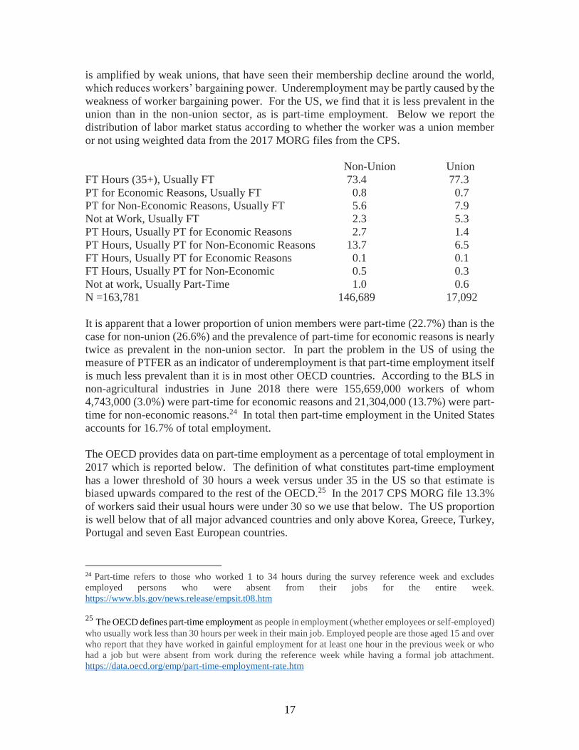
is amplified by weak unions, that have seen their membership decline around the world,

which reduces workers’ bargaining power. Underemployment may be partly caused by the

weakness of worker bargaining power. For the US, we find that it is less prevalent in the

union than in the non-union sector, as is part-time employment. Below we report the

distribution of labor market status according to whether the worker was a union member

or not using weighted data from the 2017 MORG files from the CPS.

Non-Union Union

FT Hours (35+), Usually FT 73.4 77.3

PT for Economic Reasons, Usually FT 0.8 0.7

PT for Non-Economic Reasons, Usually FT 5.6 7.9

Not at Work, Usually FT 2.3 5.3

PT Hours, Usually PT for Economic Reasons 2.7 1.4

PT Hours, Usually PT for Non-Economic Reasons 13.7 6.5

FT Hours, Usually PT for Economic Reasons 0.1 0.1

FT Hours, Usually PT for Non-Economic 0.5 0.3

Not at work, Usually Part-Time 1.0 0.6

N =163,781 146,689 17,092

It is apparent that a lower proportion of union members were part-time (22.7%) than is the

case for non-union (26.6%) and the prevalence of part-time for economic reasons is nearly

twice as prevalent in the non-union sector. In part the problem in the US of using the

measure of PTFER as an indicator of underemployment is that part-time employment itself

is much less prevalent than it is in most other OECD countries. According to the BLS in

non-agricultural industries in June 2018 there were 155,659,000 workers of whom

4,743,000 (3.0%) were part-time for economic reasons and 21,304,000 (13.7%) were part-

time for non-economic reasons.24 In total then part-time employment in the United States

accounts for 16.7% of total employment.

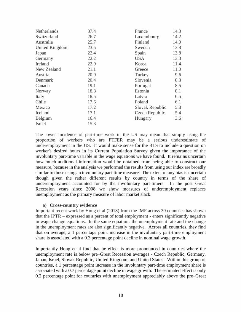
The OECD provides data on part-time employment as a percentage of total employment in

2017 which is reported below. The definition of what constitutes part-time employment

has a lower threshold of 30 hours a week versus under 35 in the US so that estimate is

biased upwards compared to the rest of the OECD.25 In the 2017 CPS MORG file 13.3%

of workers said their usual hours were under 30 so we use that below. The US proportion

is well below that of all major advanced countries and only above Korea, Greece, Turkey,

Portugal and seven East European countries.

24 Part-time refers to those who worked 1 to 34 hours during the survey reference week and excludes

employed persons who were absent from their jobs for the entire week.

https://www.bls.gov/news.release/empsit.t08.htm

25 The OECD defines part-time employment as people in employment (whether employees or self-employed)

who usually work less than 30 hours per week in their main job. Employed people are those aged 15 and over

who report that they have worked in gainful employment for at least one hour in the previous week or who

had a job but were absent from work during the reference week while having a formal job attachment.

https://data.oecd.org/emp/part-time-employment-rate.htm

18

Netherlands 37.4 France 14.3

Switzerland 26.7 Luxembourg 14.2

Australia 25.7 Finland 14.0

United Kingdom 23.5 Sweden 13.8

Japan 22.4 Spain 13.8

Germany 22.2 USA 13.3

Ireland 22.0 Korea 11.4

New Zealand 21.1 Greece 11.0

Austria 20.9 Turkey 9.6

Denmark 20.4 Slovenia 8.8

Canada 19.1 Portugal 8.5

Norway 18.8 Estonia 8.1

Italy 18.5 Latvia 6.5

Chile 17.6 Poland 6.1

Mexico 17.2 Slovak Republic 5.8

Iceland 17.1 Czech Republic 5.4

Belgium 16.4 Hungary 3.6

Israel 15.3

The lower incidence of part-time work in the US may mean that simply using the

proportion of workers who are PTFER may be a serious underestimate of

underemployment in the US. It would make sense for the BLS to include a question on

worker's desired hours in its Current Population Survey given the importance of the

involuntary part-time variable in the wage equations we have found. It remains uncertain

how much additional information would be obtained from being able to construct our

measure, because in the analysis we performed the results from using our index are broadly

similar to those using an involuntary part-time measure. The extent of any bias is uncertain

though given the rather different results by country in terms of the share of

underemployment accounted for by the involuntary part-timers. In the post Great

Recession years since 2008 we show measures of underemployment replaces

unemployment as the primary measure of labor market slack.

a) Cross-country evidence

Important recent work by Hong et al (2018) from the IMF across 30 countries has shown

that the IPTR – expressed as a percent of total employment - enters significantly negative

in wage change equations. In the same equations the unemployment rate and the change

in the unemployment rates are also significantly negative. Across all countries, they find

that on average, a 1 percentage point increase in the involuntary part-time employment

share is associated with a 0.3 percentage point decline in nominal wage growth.

Importantly Hong et al find that he effect is more pronounced in countries where the

unemployment rate is below pre–Great Recession averages - Czech Republic, Germany,

Japan, Israel, Slovak Republic, United Kingdom, and United States. Within this group of

countries, a 1 percentage point increase in the involuntary part-time employment share is

associated with a 0.7 percentage point decline in wage growth. The estimated effect is only

0.2 percentage point for countries with unemployment appreciably above the pre–Great

19

Recession averages. The authors conclude that "involuntary part-time employment

appears to have weakened wage growth even in economies where headline unemployment

rates are now at, or below, their averages in the years leading up to the recession."

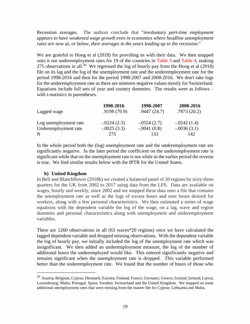
We are grateful to Hong et al (2018) for providing us with their data. We then mapped

onto it our underemployment rates for 19 of the countries in Table 3 and Table 4, making

275 observations in all.26 We regressed the log of hourly pay from the Hong et al (2018)

file on its lag and the log of the unemployment rate and the underemployment rate for the

period 1998-2016 and then for the period 1998-2007 and 2008-2016. We don't take logs

for the underemployment rate as there are nineteen negative values mostly for Switzerland.

Equations include full sets of year and country dummies. The results were as follows –

with t-statistics in parentheses.

1998-2016 1998-2007 2008-2016

Lagged wage .9198 (70.9) .9447 (24.7) .7873 (20.2)

Log unemployment rate -.0224 (2.3) -.0554 (2.7) -.0242 (1.4)

Underemployment rate -.0025 (3.3) -.0041 (0.8) -.0036 (3.1)

N 275 133 142

In the whole period both the (log) unemployment rate and the underemployment rate are

significantly negative. In the later period the coefficient on the underemployment rate is

significant while that on the unemployment rate is not while in the earlier period the reverse

is true. We find similar results below with the IPTR for the United States.

b) United Kingdom

In Bell and Blanchflower (2018b) we created a balanced panel of 20 regions by sixty-three

quarters for the UK from 2002 to 2017 using data from the LFS. Data are available on

wages, hourly and weekly, since 2002 and we mapped these data onto a file that contains

the unemployment rate as well as the logs of excess hours and over hours desired for

workers, along with a few personal characteristics. We then estimated a series of wage

equations with the dependent variable the log of the wage, on a lag, wave and region

dummies and personal characteristics along with unemployment and underemployment

variables.

There are 1260 observations in all (63 waves*20 regions) once we have calculated the

lagged dependent variable and dropped missing observations. With the dependent variable

the log of hourly pay, we initially included the log of the unemployment rate which was

insignificant. We then added an underemployment measure, the log of the number of

additional hours the underemployed would like. This entered significantly negative and

remains significant when the unemployment rate is dropped. This variable performed

better than the underemployment rate. We found that the number of hours of those who

26 Austria; Belgium; Cyprus; Denmark; Estonia; Finland; France; Germany; Greece; Iceland; Ireland; Latvia;

Luxembourg; Malta; Portugal; Spain; Sweden; Switzerland and the United Kingdom. We mapped on some

additional unemployment rates that were missing from the master file for Cyprus; Lithuania and Malta.

20

wanted more hours played no role in wage determination. The results are the same using

weekly wages. The Phillips curve in the UK, we argue, has now to be rewritten into wage

underemployment space.

c) United States

We explore the issue of underemployment reducing wage pressure further for the United

States where we only have data on PTFER available. The extent of any bias of not having

continuous excess hours variables, remains unresolved.

In Table 6 we report the result of estimating a series of log hourly wage equations on

balanced US state year panels from 1980 through 2017, using state level data from the BLS

matched by state and year to data from the Merged Outgoing Rotation Group (MORG)

files of the Current Population Survey. So, the number of observations is 1938 (50 states

+ DC * 38 years). We take the micro data in each year and collapse it to the state*year cell

to calculate hourly wages as well as personal characteristics including schooling, age, race

and gender. We also calculate the proportion of workers who say they are part-time for

economic reasons as a proportion of total employment by state (U7) from the MORG files

from 1979 through 2002; after that we use the publicly available BLS data. The personal

controls are measured across all individuals while the wage data is calculated for

employees only and part-time for economic reasons variables are calculated for all workers.

We map that onto state level data by year from the BLS on the unemployment rate (U3) as

well as data on U4 through U6, which are alternative measure of labor market slack, from

2003 through 2017.27 We then calculate one-year lagged hourly wage variable for each

state which means we lose the 1979 data.

27 The various measures are calculated as follows - the numbers refer to seasonally adjusted data for July

2018. Numbers in thousands as follows - labor force=162,245; employment=155,965;

unemployment=6,280; PTFER=4,567; discouraged workers=512 and marginally attached (which includes

discouraged workers) =1,498.

U-3=Total unemployed, as a percent of the civilian labor force (official unemployment rate) = 6280 /

(162245) =3.9%.

U-4=Total unemployed plus discouraged workers, as a percent of the civilian labor force plus discouraged

workers= (6280+512) / (162245+512) = 4.2%.

U-5=Total unemployed, plus discouraged workers, plus all other persons marginally attached to the labor

force, as a percent of the civilian labor force plus all persons marginally attached to the labor force =

(6280+1498) / (162245+1498) = 4.8%

U-6=Total unemployed, plus all persons marginally attached to the labor force, plus total employed part time

for economic reasons, as a percent of the civilian labor force plus all persons marginally attached to the labor

force = (6280+1498+4567) / (162245+1498) = 7.5%.

U7=PTFR/Employed=4567 / 155965=2.9%.

U8=discouraged / (labor force + discouraged) = 512 / (162245+512) = 0.3%

U9=marginally attached-discouraged / (labor force + marginally attached minus discouraged) = 1498-512 /

(162295 + 1498-512) = 0.9%

Persons marginally attached to the labor force are those who currently are neither working nor looking for

work but indicate that they want and are available for a job and have looked for work sometime in the past

12 months. Discouraged workers, a subset of the marginally attached, have given a job-market related reason

for not currently looking for work. Persons employed part time for economic reasons are those who want

and are available for full-time work but have had to settle for a part-time schedule.

https://www.bls.gov/news.release/empsit.t15.htm

21

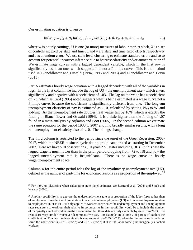
Our estimating equation is given by:

ln(𝑤𝑖𝑡) = 𝛽0 + 𝛽1 ln(𝑤𝑖𝑡−1) + 𝛽2𝑙𝑛(𝑈𝑖𝑡) + 𝛽3𝑋𝑖𝑡 + 𝜇𝑖 + 𝜈𝑡 + 𝜀𝑖𝑡 (3)

where w is hourly earnings, U is one (or more) measures of labour market slack, X is a set

of controls indexed by state and time, μ and ν are state and time fixed effects respectively

and ε is a random error. We use state level clustering to estimate standard errors and so to

account for potential incorrect inference due to heteroscedasticity and/or autocorrelation.28

We estimate wage curves with a lagged dependent variable, which in the first row is

significantly less than one, which suggests it is not a Phillips curve. This is the method

used in Blanchflower and Oswald (1994, 1995 and 2005) and Blanchflower and Levin

(2015).

Part A estimates hourly wage equation with a lagged dependent with all of the variables in

logs. In the first column we include the log of U3 – the unemployment rate - which enters

significantly and negative with a coefficient of -.03. The lag on the wage has a coefficient

of .73, which as Card (1995) noted suggests what is being estimated is a wage curve not a

Phillips curve, because the coefficient is significantly different from one. The long-run

unemployment elasticity of pay is estimated as -.10, calculated by setting Wt-1 to Wt and

solving. As the unemployment rate doubles, real wages fall by 10%, which is exactly the

finding in Blanchflower and Oswald (1994). It is a little higher than the finding of -.07

found in a meta-analysis by Nijkamp and Poot (2005). In the second column we estimate

the same equation for the period 1980 to 2007 and find broadly similar results, with a long

run unemployment elasticity also of -.10. Then things change.

The third column is restricted to the period since the onset of the Great Recession, 2008-

2017, which the NBER business cycle dating group categorized as starting in December

2007. Here we have 510 observations (10 years * 51 states including DC). In this case the

lagged wage is much lower than in the prior period dropping from .72 to .18 and now the

logged unemployment rate is insignificant. There is no wage curve in hourly

wage/unemployment space.

Column 4 for the entire period adds the log of the involuntary unemployment rate (U7),

defined as the number of part-time for economic reasons as a proportion of the employed.29

28 For more on clustering when calculating state panel estimates see Bertrand et al (2004) and Stock and

Watson (2008).

29 Another possibility is to express the underemployment rate as a proportion of the labor force rather than

of employment. We decided to separate out the effects of unemployment (U3) and underemployment relative

to employment (U7) as PTFER only applies to workers so we enter the underemployment and unemployment

rates separately to work out their relative importance. A further possibility would be to include the number

of marginally attached workers in the denominator, but these data are only available by state from 2003. The

results are very similar whichever denominator we use. For example, in column 7 of part B of Table 6 the

coefficient on U7 when the denominator is employment is -.0235 (t=2.4), when the denominator is the labor

force the coefficient is -.0212 (t=2.2) and -.0217 (t=2.2) if it is the labor force plus marginally attached

workers.

22

That variable enters significantly negative and halves the coefficient on the unemployment

rate as compared with column 1.

Column 5 is for 2008 through 2017 and is broadly similar to the previous column where

both the involuntary and unemployment rates are significantly negative. Column 6 is for

the post-recession period and only the involuntary part-time rate variable U7 is significant,

and negative while the unemployment rate is not significant. There is a wage curve in

wage underemployment space but not in wage unemployment space with a wage

underemployment elasticity of -.03. The underemployment rate here measured as PTFER

as a percent of total employment replaces the unemployment rate as the main measure of

labor market slack in the US.

In part B we experiment with alternative unemployment measures, which are available

from the BLS by state from 2003-2017 and there are 765 observations (51 * 15 years). In

the first column we include the log of the U6 measure, which also enters negatively and

significant for 2003-2017. That gives a long-run wage unemployment elasticity of -.04.

In the second column we include U7 which drives U6 to insignificance and is significant

on its own in column 3. It also gives a long-term wage underemployment elasticity of -

.04. In the fourth column we include the log of U3 as well which is insignificant while the

log of U7 remains significant and negative. So, there is a wage curve in wage *

underemployment space but not in wage * unemployment space. The fourth column

includes two further variables, in logs, we call U8 which identifies the discouraged worker

rate, which is measured as discouraged / (labor force + discouraged), and U9 which

identifies the number of marginally attached minus the number of discouraged workers,

which is measured as marginally attached-discouraged / (labor force + marginally attached

- discouraged). The coefficients on both are insignificant in column 4. The final four

columns of part B are restricted to the post-recession period of 2008-2017 (n=510 – 10

years * 51 states). The underemployment measure U7 is always significantly negative.

Discouraged worker and marginally attached worker rates are thus irrelevant in the wage

determination process.

Table 7 does the same as in Table 6 but this time for weekly wages and the results are very

similar. Here we find that the log unemployment rate remains significant in part A until

the Involuntary PT variable U7 is added. The long run wage/unemployment elasticity is

in column 1 is estimated at -.12; -.11 in column 2 and -.06 in column 3. Adding the

significant and negative involuntary part-time variable in columns 4 through 6 removes the

size of the coefficient on the log unemployment rate. In part B the log U6 variable

generates an elasticity of -.09 in column 1 but then becomes insignificant once U7 is

included. Including the U7 variable, in column 3 gives a wage underemployment elasticity

of -.08. For the later period in column 7 the elasticity is -.07. Wage responses to labor

market shocks in the later period are less than in pre-recession period and come through

the underemployment rate whereas in the earlier period they come through both the

unemployment rate and the underemployment rate.

23

These results are entirely consistent with those reported in a new paper by Bracha and

Burke (2018) from the Federal Reserve Bank of Boston. They find that hidden labor

market slack in the form of informal ‘‘gig’’ economy work helps to explain the benign

wage puzzle. They argue that informal work represents additional labor market slack.

They focus on informal work that is labor-intensive, in the Survey of Informal Work

Participation for 2015–2016. The SIWP is an annual module within the Federal Reserve

Bank of New York’s Survey of Consumer Expectations. A respondent is defined as an

informal worker if he or she (1) indicated working in at least one informal paid activity that

is not survey work or renting/selling activities, and (2) reported strictly positive hours

considering all activities except surveys and renting/selling. According to this measure,

19% of the individuals in their analysis sample (averaged over the three survey waves) are

classified as informal workers. They find that informal labor is negatively associated with

wage growth at the census division level, while no such association exists between wage

growth and unemployment rates, whether defined as U3 or U6.

Table 8 builds on work by Blanchflower and Oswald (2013) and discussed in Blanchflower

(2019) on the home ownership rate, which finds that a lagged home ownership rate was a

significant predictor of unemployment rate. A five-year lag on the home ownership rate

enters positively into unemployment equations. A higher home ownership rate in a state

also lowered mobility. It is notable that the home ownership rate has declined steadily

from its peak in 2004.30 According to the Census Bureau home ownership rates reached a

peak of 69.4% in the second quarter of 2004 and fell steadily through the second quarter

of 2016 to 63.1% but have risen since then to 64.2% in the first quarter of 2018. In the

table, which is split into two parts, for hourly and weekly wages respectively, we examine

the impact of changes in the home ownership rate impacts wage growth. In the period

1980-2007 annual change in the home ownership rate averaged +0.1% per annum. In the

years 2008-2017 it averaged -0.4%. Every year from 2005-2016 was the change in home

ownership was negative while in 2017 it turned positive again. We report results separately

again for hourly and weekly wages.

In part A for hourly wages we include the log change in the home ownership rate, which

enters significantly positive in columns 5 and 6 post-2008 but is insignificant in the pre-

recession years in columns 1-4. A falling home ownership rate lowers wage pressure in

the pre-recession years. The involuntary part-time variable U7 are significant again and

the unemployment rate, whether measured as U6 or U3 are not. The results are very similar

for weekly wages although there is evidence that the change in home ownership rate

variable enters positively for the whole period 1980-2017 and for the pre- and post-

recession periods. A rising home ownership rate pre-recession raises weekly wages in the

30 According to the Census Bureau annual home ownership rates – averaging across the seasonally adjusted

four quarters were = 1980=65.6%; 1981=65.4; 1982=64.8; 1983=64.7; 1984=64.5; 1985=63.9; 1986=63.8;

1987=64.0; 1988=63.8; 1989=63.9; 1990=64.0; 1991=64.1; 1992=64.2; 1993=64.0; 1994=64.0; 1995=64.8;

1996=65.4; 1997=65.7; 1998=66.3; 1999=66.8; 2000=67.4; 2001=67.8; 2002=68.0; 2003=68.3; 2004=69.0;

2005=68.9; 2006=68.8; 2007=68.2; 2008=67.8; 2009=67.4; 2010=66.9; 2011=66.1; 2012=65.5; 2013=65.2;

2014=64.5; 2015=63.7; 2016=63.4; 2017=63.9.

https://www.census.gov/housing/hvs/data/histtabs.html

24

early period and a falling rate lowers them in the second. So, falling home ownership in

the post-recession years in the USA contributed to slowing wage growth.

So, what?

In the post-recession period underemployment has replaced unemployment as the main

indicator of labor market slack. Underemployment has not returned to its pre-recession

level in many countries, whereas unemployment has. In the past, at the low levels of the

unemployment rate existing in countries like the US, Germany, the United states, speaking

there was a pay norm of 4% in the years before the Great Recession and 2% subsequently.

As a consequence, underemployment is pushing down on wages while the unemployment

rate contains little or no information on wage pressure at such low levels in either the UK

or the USA. The unemployment rate is having no impact on wages after the Great

Recession whereas it did before.

Even though the unemployment rate is at historic lows in many countries this still does not

suggest that these country's labor markets are anywhere close to full-employment. In his

1944 book Full Employment in a Free Society William Beveridge argued that 'full

employment means that unemployment is reduced to short intervals of standing by, with

the certainty that very soon one will be wanted in one's old job again or will be wanted in

a new job that is within one's powers'. (p.18). In his 1960 prologue he wrote that "full

employment means having more vacancies for workers than there are workers seeking

vacancies. It does not mean having no unemployment at all." Full employment likely does

not mean excessively high underemployment rates where workers are willing to work more

hours at the going wage.

Policymakers should not be focused on the unemployment rate in the years post-recession

but rather on the underemployment rate. Declining home ownership has also helped to

contain wage growth. We have shown there is a relatively flat wage curve in

wage*underemployment space in the post-recession years in the United States but not one

in wage*unemployment space. This helps to explain the low wage growth as

underemployment remains elevated. Underemployment replaces unemployment as the

main measure of labor market slack in the post-recession years.

25

References

Ashenfelter, Orley C., Henry Farber, and Michael R. Ransom. 2010. Labor market

monopsony. Journal of Labor Economics 28(2): 203–210.

José A. Azar, Ioana Marinescu, Marshall I. Steinbaum and Bledi Taska. 2017. Labor

market concentration, NBER Working paper #24147.

Ball, Robert J. and Eric B.A. St Cyr. 1966. Short-term employment functions in British

manufacturing industry. Review of Economic Studies 33(3), July: 179-207.

Bell, David N.F. and David G. Blanchflower. 2018a. The lack of wage growth and the

falling NAIRU. National Institute Economic Review 245(1): R1-R16.

Bell, David N.F. and David G. Blanchflower. 2018b. The well-being of the overemployed

and the underemployed and the rise in depression in the UK. NBER Working paper

#24840.

Bell, David N.F. and David G. Blanchflower. 2018c. Underemployment and the lack of

wage pressure in the UK. National Institute Economic Review 243(1): R53-R61.

Bell, David N.F. and David G. Blanchflower. 2014. Labor market slack in the UK.

National Institute Economic Review 229(1): F4-F11.

Bell, David N.F. and David G. Blanchflower. 2013. Underemployment in the UK revisited.

National Institute Economic Review 224(1): F8-F22.

Bell, David N.F. and David G. Blanchflower. 2011. Youth underemployment in the UK in

the Great Recession. National Institute Economic Review 215(1): R1-R11.

Bertrand, Marianne. Esther Duflo and Sendhil Mullainathan. 2004. How much should we

trust differences-in-differences estimates? The Quarterly Journal of Economics 119(1):

249–275.

Bhaskar, Venkataraman, Alan Manning and Ted To 2002. Oligopsony and monopsonistic

competition in labor markets. Journal of Economic Perspectives 16(2):155-174.

Blanchflower, David G. 2019. Not Working: Where Have All The Good Jobs Gone?

Princeton University Press, Princeton, NJ.

Blanchflower, David G. 2015. As good as it gets? The UK labor market in recession and

recovery. National Institute Economic Review 231, February: F76-F80.

Blanchflower, David G. and Andrew T. Levin 2015. Labor market slack and monetary

policy. NBER working paper #21094.

26

Blanchflower, David G. and Andrew J, Oswald. 2013. Does high home ownership impair

the labor market? NBER Working Paper #W19079.

Blanchflower, David G. and Andrew J, Oswald. 2005. The wage curve reloaded’. NBER

Working Paper #11338.

Blanchflower, David G. and Andrew J, Oswald. 1995. An introduction to the wage curve.

Journal of Economic Perspectives 9(3):153-67.

Blanchflower, David G. and Andrew J, Oswald. 1994. The Wage Curve. MIT Press,

Cambridge, MA.

Borowczyk-Martins, Daniel. and Etienne Lalé. 2018. The welfare effects of involuntary

part-time work. Oxford Economic Papers 70(1): 183–205,

Borowczyk-Martins, Daniel, and Etienne Lalé. 2016. Employment adjustment and Part-

time work: lessons from the United States and the United Kingdom. IZA WP #9847,

March.

Bracha, Anat and Mary A. Burke. 2018. Wage inflation and informal work. Economics

Letters 171: 159–163.

Brechling, Frank P.R. 1965. The relationship between output and employment in British

manufacturing. Review of Economic Studies 32(3): 187-216.

Cajner, Tomaz, Dennis Mawhirter, Christopher Nekarda and David Ratner 2014. Why is

involuntary part-time work elevated? FEDS Notes, Board of Governors of the Federal

Reserve, April 14th.

Card, David. 1995. The wage curve: a review. Journal of Economic Literature 33(2): 785-

799.

Card, David, Ana R. Cardoso, Joerg Heining and Patrick Kline. 2018. Firms and labor

market inequality: evidence and some theory. Journal of Labor Economics 36 (S1): S13-

S70.

Depew, Briggs, and Todd A. Sørensen (2013). The elasticity of labor supply to the firm

over the business cycle, Labour Economics 24(1): 196–204.

Feather, Peter M., and W. Douglass Shaw. 2000. The demand for leisure time in the

presence of constrained work hours. Economic Inquiry 38(4): 651-661.

Feldstein, Martin S. 1967. Specification of the labour input in the aggregate production

function. The Review of Economic Studies 34(4): 375-386.

27

Glauber, Rebecca. 2017. Involuntary part-time employment. A slow and uneven economic

recovery. Carsey Research National Issue Brief #116, University of New Hampshire,

Spring.

Golden, Lonnie. 2016. Still falling short on hours and pay. Employment Policy Institute

Report, December 5th.

Golden, Lonnie and Tesfayi Gebreselassie. 2007. Overemployment mismatches: the

preference for fewer work hours. Monthly Labor Review April:18-37.

Hart, Robert A. 2017. Hours vs employment in response to demand shocks. IZA World of

Labor, 393, October.

Hart, Robert A. and Trevor Sharot. 1978. The short-run demand for workers and hours: a

recursive model. Review of Economic Studies 45(2): 299-309.

Hirsch, Boris, Elke J. Jahn, and Claus Schnabel. 2018. Do employers have more

monopsony power in slack labor markets? Industrial and Labor Relations Review 71(3):

676–704

Hong, Gee H., Zsoka Kóczán, Weicheng Lian, and Malhar S. Nabar (2018), ‘More slack

than meets the eye? Recent wage dynamics in advanced economies,’ IMF Working Paper

/18/50, IMF Research Department.

Hurley, John and Valentina Patrini. 2017. Estimating labor market slack in Europe.

European Foundation for the Improvement of Living and Working Conditions,

Hwang, Hae-shin S., Mortensen, Dale T., and Reed, W. Robert 1998. Hedonic wages and

labor market search. Journal of Labor Economics 16(4): 815-847.

Lewis, H. Gregg. 1957. Hours of work and hours of leisure. Paper presented at the

Proceedings of the Ninth Annual Meeting of the Industrial Relations Research Association,

Madison, WI: 196–206.

Lewis, H. Gregg. 1969. Employer interests in employee hours of work. Cuadernos de

Economia 6(18):38–54.

Lundberg, Shelley 1985. Tied wage-hours offers and the endogeneity of wages. Review of

Economics and Statistics 67(3): 405-410.

Manning, Alan. 2003. Monopsony in Motion. Princeton University Press, Princeton, NJ:

Nijkamp, Peter, and Jacques Poot. 2005. The last word on the wage curve? Journal of

Economic Surveys 19(3): 421-450.

28

Pencavel, John. 1986. Labor supply of men: a survey. Handbook of Labor Economics,

edited by Orley Ashenfelter and David Card, volume 1: 3-102.

Pencavel, John. 2016. Whose preferences are revealed in hours of work? Economic Inquiry

54(1): 9-24.

Pencavel, John. 2018. Diminishing Returns At Work. Oxford University Press, Oxford.

Quévat, Benjamin and Benjamin Vignolles. 2018. The relationships between inflation,

wages and unemployment have not disappeared. A comparative study of the French and

American economies. INSEE, Conjoncture in France, March.

https://www.insee.fr/en/statistiques/3372431?sommaire=3372475&q=earnings

Rosen, Sherwin. 1969. On the interindustry wage and hours structure. Journal of Political

Economy 77(2): 249-273.

Springford, John. 2018. The German wage puzzle. Insight, Centre for European Reform, May.

Stock, James. H. and Mark W. Watson. 2008. Heteroskedasticity‐robust standard errors for

fixed effects panel data regression. Econometrica 76(1):155-174.

Stole, Lars A. and Jeffrey Zwiebel. 1996. Intra-firm Bargaining under Non-binding

Contracts. Review of Economic Studies 63(3): 375-410.

Sum, Andrew and Ishwar Khatiwada. 2010. The nation's underemployed in the 'Great

Recession' of 2007-2009. Monthly Labor Review November: 3-15.

Valletta, Robert G, Leila Bengali and Catherine van der List. 2018. Cyclical and market

determinants of involuntary part-time employment. Federal Reserve Bank of San Francisco

Working Paper 2015-19.

Veliziotis, Michail, Manos Matsaganis and Alexandros Karakitsios. 2015. Involuntary

part-time employment: perspectives from two European labor markets. Improve

Discussion Paper 15/2 January.

Walling, Annette. 2007. Understanding statistics on full-time/part-time employment.

Economic and Labor Market Review 1(2), February: 36-43.

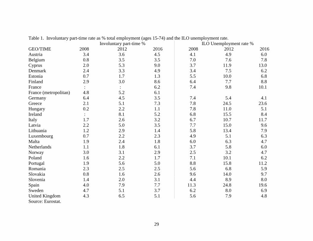
29

Table 1. Involuntary part-time rate as % total employment (ages 15-74) and the ILO unemployment rate.

Involuntary part-time % ILO Unemployment rate %

GEO/TIME 2008 2012 2016 2008 2012 2016

Austria 3.4 3.6 4.5 4.1 4.9 6.0

Belgium 0.8 3.5 3.5 7.0 7.6 7.8

Cyprus 2.0 5.3 9.0 3.7 11.9 13.0

Denmark 2.4 3.3 4.9 3.4 7.5 6.2

Estonia 0.7 1.7 1.3 5.5 10.0 6.8

Finland 2.9 3.0 8.6 6.4 7.7 8.8

France : : 6.2 7.4 9.8 10.1

France (metropolitan) 4.8 5.2 6.1

Germany 6.4 4.5 3.5 7.4 5.4 4.1

Greece 2.1 5.1 7.3 7.8 24.5 23.6

Hungary 0.2 2.2 1.1 7.8 11.0 5.1

Ireland : 8.1 5.2 6.8 15.5 8.4

Italy 1.7 2.6 3.2 6.7 10.7 11.7

Latvia 2.2 5.0 3.5 7.7 15.0 9.6

Lithuania 1.2 2.9 1.4 5.8 13.4 7.9

Luxembourg 0.7 2.2 2.3 4.9 5.1 6.3

Malta 1.9 2.4 1.8 6.0 6.3 4.7

Netherlands 1.1 1.8 6.1 3.7 5.8 6.0

Norway 3.0 3.1 2.9 2.5 3.2 4.7

Poland 1.6 2.2 1.7 7.1 10.1 6.2

Portugal 1.9 5.6 5.0 8.8 15.8 11.2

Romania 2.3 2.5 2.5 5.6 6.8 5.9

Slovakia 0.8 1.6 2.6 9.6 14.0 9.7

Slovenia 1.4 2.0 3.1 4.4 8.9 8.0

Spain 4.0 7.9 7.7 11.3 24.8 19.6

Sweden 4.7 5.1 3.7 6.2 8.0 6.9

United Kingdom 4.3 6.5 5.1 5.6 7.9 4.8

Source: Eurostat.

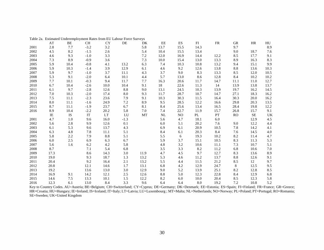
30

Table 2a. Estimated Underemployment Rates from EU Labour Force Surveys

AT BE CH CY DE DK EE ES FI FR GR HR HU

2001 2.8 7.7 -3.2 3.2 5.8 13.7 15.5 14.3 9.7 8.9

2002 4.5 8.2 -1.5 2.6 5.4 10.4 15.5 13.4 9.0 18.7 7.6

2003 4.6 9.3 -1.0 3.3 7.2 12.0 16.9 14.4 12.2 8.5 17.7 9.1

2004 7.3 8.9 -0.9 3.6 7.3 10.0 15.4 13.0 13.3 8.9 16.3 8.3

2005 5.9 10.4 -0.8 4.1 13.2 6.3 7.4 10.3 10.8 13.2 9.4 15.1 9.9

2006 5.9 10.3 -1.4 3.9 12.9 6.1 4.6 9.2 12.6 13.8 8.8 13.6 10.3

2007 5.9 9.7 -1.0 3.7 11.1 4.3 3.7 9.0 8.3 13.3 8.5 12.0 10.5

2008 5.3 9.1 -2.0 6.4 10.1 4.4 5.7 13.0 8.6 12.8 8.4 10.2 10.2

2009 7.7 10.1 -0.3 9.4 11.7 7.7 16.3 20.6 11.7 14.7 11.1 11.0 12.7

2010 6.7 10.4 -2.6 10.0 10.4 9.1 18 22.6 11.3 14 13.9 13.8 13.7

2011 6.1 9.7 -2.8 12.6 8.8 9.0 13.1 24.5 10.3 13.9 19.7 16.2 14.5

2012 7.0 10.3 -2.0 17.4 8.0 9.3 11.7 28.7 10.7 14.7 27.1 18.3 16.2

2013 7.5 11.1 -2.3 23.6 7.9 9.1 10.3 30.3 11.5 16.4 30.3 20.0 16.2

2014 8.0 11.1 -1.6 24.9 7.2 8.9 9.5 28.5 12.2 16.6 29.8 20.3 13.5

2015 8.7 11.1 -1.9 23.7 6.7 8.1 8.4 25.6 13.4 16.5 28.4 19.8 12.2

2016 8.9 10.4 -2.2 20.2 5.8 7.0 7.4 22.7 11.9 15.7 26.8 15.7 9.1

IE IS IT LT LU MT NL NO PL PT RO SE UK

2001 4.7 1.0 9.6 16.0 -1.3 5.6 4.7 18.1 6.0 12.9 4.5

2002 5.6 2.8 9.9 12.6 0.1 6.0 5.1 20.2 7.6 9.0 12.2 4.4

2003 6.1 5.3 9.6 13.7 4.3 6.9 6.1 20.9 10.5 7.8 14.2 4.1

2004 6.3 4.8 7.8 11.1 5.1 8.4 6.1 20.3 8.4 7.6 14.5 4.0

2005 5.8 2.2 7.9 8.8 5.1 5.5 6 19.3 10.2 8.2 11.4 4.7

2006 6.0 2.5 6.9 6.3 6.7 5.9 3.7 15.1 10.5 8.3 11.3 5.3

2007 5.6 1.6 6.2 4.2 5.8 4.8 3.2 10.6 11.1 7.3 10.7 5.1

2008 8.7 7.1 5.4 6.8 3.5 3.3 8.2 11.2 6.8 10.6 7.0

2009 17.3 8.6 14.3 3.0 11.9 4.7 4.5 9.7 12.7 8.3 13.6 8.9

2010 19.0 9.3 18.7 1.3 13.2 5.3 4.6 11.2 13.7 8.8 12.6 9.1

2011 20.4 9.2 16.4 2.1 13.2 5.5 4.4 11.5 21.2 8.5 12 9.7

2012 20.8 12.1 14.6 1.7 13.1 6.8 4.2 12.9 24.7 8 12.5 9.5

2013 19.2 13.6 13.0 3.0 12.9 9.0 5.2 13.9 25.1 8.2 12.8 8.5

2014 16.9 9.1 14.2 12.1 2.5 12.6 8.8 5.0 12.3 22.8 8.4 12.9 6.8

2015 14.6 7.5 13.3 10.1 1.5 12.2 8.2 6.0 10.0 20.4 8.5 12.3 5.8

2016 12.3 6.1 13.0 8.4 3.3 9.6 6.4 6.4 8.0 19.2 7.2 10.8 5.2

Key to Country Codes. AU=Austria; BE=Belgium; CH=Switzerland; CY=Cyprus; DE=Germany; DK=Denmark; EE=Estonia; ES=Spain; FI=Finland; FR=France; GR=Greece;

HR=Croatia; HU=Hungary; IE=Ireland; IS=Iceland; IT=Italy; LT=Latvia; LU=Luxembourg ; MT=Malta; NL=Netherlands; NO=Norway; PL=Poland; PT=Portugal; RO=Romania;

SE=Sweden; UK=United Kingdom

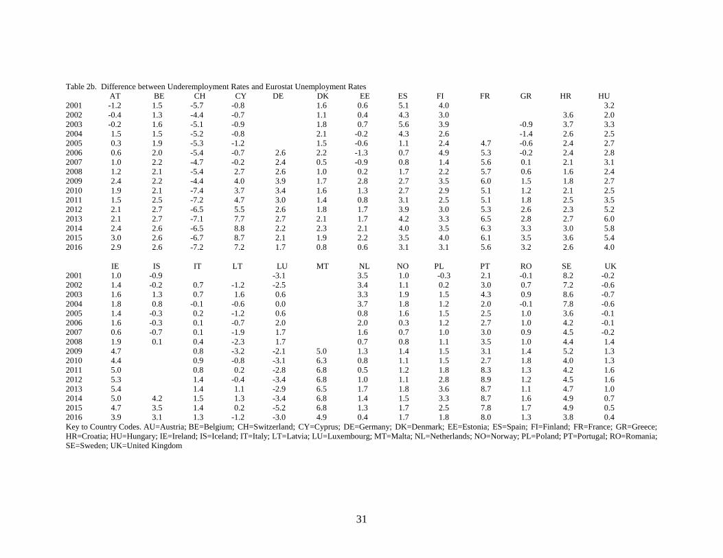
31

Table 2b. Difference between Underemployment Rates and Eurostat Unemployment Rates

AT BE CH CY DE DK EE ES FI FR GR HR HU

2001 -1.2 1.5 -5.7 -0.8 1.6 0.6 5.1 4.0 3.2

2002 -0.4 1.3 -4.4 -0.7 1.1 0.4 4.3 3.0 3.6 2.0

2003 -0.2 1.6 -5.1 -0.9 1.8 0.7 5.6 3.9 -0.9 3.7 3.3

2004 1.5 1.5 -5.2 -0.8 2.1 -0.2 4.3 2.6 -1.4 2.6 2.5

2005 0.3 1.9 -5.3 -1.2 1.5 -0.6 1.1 2.4 4.7 -0.6 2.4 2.7

2006 0.6 2.0 -5.4 -0.7 2.6 2.2 -1.3 0.7 4.9 5.3 -0.2 2.4 2.8

2007 1.0 2.2 -4.7 -0.2 2.4 0.5 -0.9 0.8 1.4 5.6 0.1 2.1 3.1

2008 1.2 2.1 -5.4 2.7 2.6 1.0 0.2 1.7 2.2 5.7 0.6 1.6 2.4

2009 2.4 2.2 -4.4 4.0 3.9 1.7 2.8 2.7 3.5 6.0 1.5 1.8 2.7

2010 1.9 2.1 -7.4 3.7 3.4 1.6 1.3 2.7 2.9 5.1 1.2 2.1 2.5

2011 1.5 2.5 -7.2 4.7 3.0 1.4 0.8 3.1 2.5 5.1 1.8 2.5 3.5

2012 2.1 2.7 -6.5 5.5 2.6 1.8 1.7 3.9 3.0 5.3 2.6 2.3 5.2

2013 2.1 2.7 -7.1 7.7 2.7 2.1 1.7 4.2 3.3 6.5 2.8 2.7 6.0

2014 2.4 2.6 -6.5 8.8 2.2 2.3 2.1 4.0 3.5 6.3 3.3 3.0 5.8

2015 3.0 2.6 -6.7 8.7 2.1 1.9 2.2 3.5 4.0 6.1 3.5 3.6 5.4

2016 2.9 2.6 -7.2 7.2 1.7 0.8 0.6 3.1 3.1 5.6 3.2 2.6 4.0

IE IS IT LT LU MT NL NO PL PT RO SE UK

2001 1.0 -0.9 -3.1 3.5 1.0 -0.3 2.1 -0.1 8.2 -0.2

2002 1.4 -0.2 0.7 -1.2 -2.5 3.4 1.1 0.2 3.0 0.7 7.2 -0.6

2003 1.6 1.3 0.7 1.6 0.6 3.3 1.9 1.5 4.3 0.9 8.6 -0.7

2004 1.8 0.8 -0.1 -0.6 0.0 3.7 1.8 1.2 2.0 -0.1 7.8 -0.6

2005 1.4 -0.3 0.2 -1.2 0.6 0.8 1.6 1.5 2.5 1.0 3.6 -0.1

2006 1.6 -0.3 0.1 -0.7 2.0 2.0 0.3 1.2 2.7 1.0 4.2 -0.1

2007 0.6 -0.7 0.1 -1.9 1.7 1.6 0.7 1.0 3.0 0.9 4.5 -0.2

2008 1.9 0.1 0.4 -2.3 1.7 0.7 0.8 1.1 3.5 1.0 4.4 1.4

2009 4.7 0.8 -3.2 -2.1 5.0 1.3 1.4 1.5 3.1 1.4 5.2 1.3

2010 4.4 0.9 -0.8 -3.1 6.3 0.8 1.1 1.5 2.7 1.8 4.0 1.3

2011 5.0 0.8 0.2 -2.8 6.8 0.5 1.2 1.8 8.3 1.3 4.2 1.6

2012 5.3 1.4 -0.4 -3.4 6.8 1.0 1.1 2.8 8.9 1.2 4.5 1.6

2013 5.4 1.4 1.1 -2.9 6.5 1.7 1.8 3.6 8.7 1.1 4.7 1.0

2014 5.0 4.2 1.5 1.3 -3.4 6.8 1.4 1.5 3.3 8.7 1.6 4.9 0.7

2015 4.7 3.5 1.4 0.2 -5.2 6.8 1.3 1.7 2.5 7.8 1.7 4.9 0.5

2016 3.9 3.1 1.3 -1.2 -3.0 4.9 0.4 1.7 1.8 8.0 1.3 3.8 0.4

Key to Country Codes. AU=Austria; BE=Belgium; CH=Switzerland; CY=Cyprus; DE=Germany; DK=Denmark; EE=Estonia; ES=Spain; FI=Finland; FR=France; GR=Greece;

HR=Croatia; HU=Hungary; IE=Ireland; IS=Iceland; IT=Italy; LT=Latvia; LU=Luxembourg; MT=Malta; NL=Netherlands; NO=Norway; PL=Poland; PT=Portugal; RO=Romania;

SE=Sweden; UK=United Kingdom

32

Table 3a. Increase in weekly hours desired by those who want more hours (millions)

AT BE CH CY DE DK EE ES FI FR GR HR HU 2001 2.6 2.9 7.5 0.6 2.1 1.4 40.2 9.2 8.1 10.0

2002 1.2 2.5 8.5 0.7 1.2 1.1 33.8 8.8 8.3 3.0 8.1

2003 1.2 2.8 7.7 0.8 2.2 1.1 45.5 9.2 53.7 8.2 3.2 10.2

2004 2.2 2.9 7.7 0.9 2.5 0.9 39.1 8.2 58.7 8.0 2.0 9.5

2005 8.3 3.5 7.5 0.7 34.8 1.9 0.6 24.8 7.0 61.0 8.0 1.8 8.7

2006 8.9 3.7 7.6 0.7 41.9 2.8 0.6 24.0 9.2 68.1 8.5 1.8 8.3

2007 9.5 4.0 8.8 0.7 39.2 6.9 0.5 23.2 7.5 73.0 8.8 1.6 8.7

2008 9.6 3.8 8.3 0.9 91.8 7.1 0.7 28.1 7.4 73.1 9.7 1.3 7.2

2009 11.1 3.9 8.8 1.1 99.8 6.8 1.3 33.8 7.7 73.3 11.1 1.4 7.1

2010 10.8 3.9 7.1 1.0 90.3 6.2 1.0 33.3 7.2 69.7 9.8 1.7 7.0

2011 10.3 4.6 7.3 1.1 82.3 5.9 0.9 35.7 7.0 67.9 10.3 1.9 8.3

2012 11.0 4.9 7.7 1.2 78.0 6.0 1.1 41.7 7.5 69.2 11.5 1.7 10.8

2013 11.0 5.0 7.7 1.6 75.0 6.2 1.2 43.4 7.6 85.3 11.7 2.0 12.3

2014 11.3 4.8 8.5 1.8 70.4 6.1 1.3 41.2 7.9 83.8 12.5 2.2 12.3

2015 12.0 4.8 8.4 1.7 66.9 5.7 1.3 36.8 8.0 82.2 13.0 2.7 11.8

2016 12.3 4.7 8.2 1.5 63.4 8.2 1.1 33.4 7.7 77.8 12.7 1.9 9.9

IE IS IT LT LU MT NL NO PL PT RO SE UK

2001 1.3 0.4 2.3 0.1 21.8 0.9 37.3 7.4 18.6 24.7

2002 1.7 0.4 6.2 2.1 0.1 22.4 0.9 38.3 8.9 19.0 17.2 24.5

2003 1.8 0.3 7.2 2.4 0.2 20.6 1.5 40.4 10.9 18.2 19.3 24.7

2004 2.3 0.2 14.9 1.9 0.2 23.2 1.6 38.2 6.7 13.9 18.0 24.0

2005 2.4 0.2 11.4 1.8 0.2 16.8 1.4 37.3 7.3 14.9 14.5 24.6

2006 2.5 0.2 11.2 1.7 0.3 19.7 4.7 36.6 7.9 13.5 15.2 26.8

2007 2.1 0.2 10.4 1.5 0.3 20.1 4.8 34.7 8.7 12.6 15.7 28.0

2008 2.8 12.0 1.2 0.3 20.7 5.2 33.6 9.6 12.4 15.6 30.0

2009 4.8 13.0 1.4 0.4 0.4 21.9 5.3 34.7 8.6 12.8 16.6 36.2

2010 4.5 12.5 1.4 0.3 0.5 19.3 4.9 33.9 7.8 12.8 15.1 39.6

2011 5.0 11.6 1.4 0.3 0.5 17.9 4.9 33.9 19.5 11.8 15.4 40.9

2012 5.4 16.3 1.5 0.4 0.6 19.0 5.2 40.3 20.5 11.4 16.1 43.1

2013 5.6 16.6 1.5 0.4 0.5 21.5 5.8 44.2 19.7 10.6 16.9 43.8

2014 5.1 0.5 18.0 1.5 0.5 0.6 20.8 5.3 41.9 20.3 11.4 17.3 44.4

2015 4.8 0.4 17.3 1.4 0.5 0.6 21.4 5.6 36.4 18.2 11.3 17.4 42.0

2016 4.3 0.4 16.7 1.3 0.5 0.5 19.8 5.5 33.0 18.4 9.7 15.7 39.7

Key to Country Codes. AU=Austria; BE=Belgium; CH=Switzerland; CY=Cyprus; DE=Germany; DK=Denmark; EE=Estonia; ES=Spain; FI=Finland; FR=France; GR=Greece;

HR=Croatia; HU=Hungary; IE=Ireland; IS=Iceland; IT=Italy; LT=Latvia; LU=Luxembourg; MT=Malta; NL=Netherlands; NO=Norway; PL=Poland; PT=Portugal; RO=Romania;

SE=Sweden; UK=United Kingdom

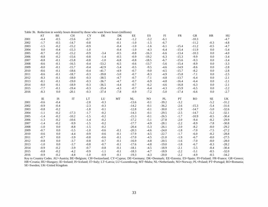
33

Table 3b. Reduction in weekly hours desired by those who want fewer hours (millions)

AT BE CH CY DE DK EE ES FI FR GR HR HU

2001 -4.4 -0.5 -15.6 -0.7 -0.4 -1.2 -3.2 -6.1 -10.3 -4.7

2002 -1.7 -0.5 -14.7 -0.8 -0.1 -1.0 -1.5 -6.7 -11.2 -0.3 -4.8

2003 -1.5 -0.2 -15.2 -0.9 -0.4 -1.0 -1.6 -6.1 -15.4 -11.2 -0.5 -4.7

2004 0.0 -0.4 -15.3 -1.0 -0.4 -1.0 -4.3 -6.4 -15.4 -11.9 0.0 -5.4

2005 -8.7 -0.2 -15.2 -0.9 -3.4 -0.5 -0.8 -16.3 -6.6 -13.4 -10.3 0.0 -4.0

2006 -8.8 -0.2 -15.6 -0.8 -1.4 -0.5 -0.9 -19.2 -6.3 -15.3 -9.9 0.0 -3.4

2007 -8.8 -0.1 -15.8 -0.8 -1.0 -6.8 -0.8 -18.5 -6.7 -15.6 -9.3 0.0 -3.4

2008 -8.6 -0.1 -16.5 -0.4 -53.2 -6.5 -0.6 -13.7 -5.6 -15.4 -8.9 0.0 -3.3

2009 -8.0 -0.1 -15.7 -0.4 -42.9 -5.4 -0.5 -9.5 -4.6 -14.9 -8.6 0.0 -2.8

2010 -8.6 -0.1 -18.6 -0.4 -41.7 -4.9 -0.7 -9.0 -4.5 -15.7 -8.2 0.0 -2.8

2011 -8.6 -0.1 -18.7 -0.3 -39.8 -5.0 -0.7 -8.3 -4.9 -15.8 -7.1 0.0 -2.5

2012 -8.3 -0.1 -18.0 -0.3 -38.5 -4.7 -0.7 -7.1 -4.8 -13.7 -6.4 0.0 -2.1

2013 -8.1 -0.1 -19.0 -0.3 -36.7 -4.7 -0.7 -6.9 -4.8 -16.4 -6.4 0.0 -2.1

2014 -8.0 -0.1 -18.9 -0.3 -36.5 -4.4 -0.7 -6.2 -4.6 -16.8 -6.3 0.0 -2.1

2015 -7.7 -0.1 -19.4 -0.3 -35.4 -4.3 -0.7 -6.4 -4.3 -15.9 -6.5 0.0 -2.2

2016 -8.3 0.0 -20.1 -0.3 -37.4 -7.8 -0.9 -7.2 -5.0 -17.4 -6.6 0.0 -2.7

IE IS IT LT LU MT NL NO PL PT RO SE UK

2001 -0.6 -0.4 -2.8 -0.3 -13.6 -0.1 -39.2 -3.2 -5.2 -31.2

2002 -0.9 -0.4 -2.3 -0.3 -14.2 -0.1 -36.2 -2.6 -15.3 -5.4 -31.6

2003 -0.8 -0.2 -1.8 -0.1 -12.8 -0.1 -30.0 -1.9 -14.7 -5.0 -32.6

2004 -1.1 -0.2 -17.3 -1.7 -0.2 -14.3 -0.1 -29.5 -2.5 -14.7 -5.2 -32.1

2005 -1.4 -0.2 -10.2 -1.5 -0.2 -15.3 -0.1 -26.5 -1.7 -10.9 -8.5 -30.4

2006 -1.3 -0.2 -10.6 -1.4 -0.2 -17.2 -5.1 -27.8 -2.0 -9.4 -8.2 -29.9

2007 -1.4 -0.2 -9.9 -1.5 -0.2 -17.7 -4.9 -28.1 -2.2 -8.9 -7.8 -30.8

2008 -1.0 0.0 -8.8 -1.5 -0.2 -20.4 -5.3 -26.1 -2.0 -8.2 -8.0 -29.2

2009 -0.7 0.0 -5.5 -1.0 -0.6 -0.1 -20.3 -4.6 -24.0 -1.8 -7.0 -7.5 -27.2

2010 -0.6 0.0 -4.4 -0.9 -0.6 -0.1 -17.9 -4.5 -22.7 -1.7 -6.0 -8.2 -28.8

2011 -0.7 0.0 -3.9 -0.8 -0.6 -0.1 -17.0 -4.5 -21.0 -1.9 -6.7 -8.0 -27.5

2012 -0.8 0.0 -3.7 -0.8 -0.7 -0.1 -16.9 -4.8 -20.5 -1.6 -7.0 -8.0 -28.0

2013 -1.0 0.0 -3.7 -0.8 -0.7 -0.1 -17.6 -4.8 -19.0 -1.8 -6.7 -8.3 -28.2

2014 -0.9 -0.2 -3.9 -0.7 -0.8 -0.1 -18.1 -4.5 -18.9 -2.1 -5.5 -8.4 -30.4

2015 -0.8 -0.2 -4.2 -0.9 -1.1 -0.1 -18.3 -4.7 -18.9 -2.2 -5.1 -8.5 -32.0

2016 -0.9 -0.2 -4.8 -1.0 -0.9 -0.1 -19.3 -4.3 -20.0 -2.2 -4.9 -8.5 -34.2

Key to Country Codes. AU=Austria; BE=Belgium; CH=Switzerland; CY=Cyprus; DE=Germany; DK=Denmark; EE=Estonia; ES=Spain; FI=Finland; FR=France; GR=Greece;

HR=Croatia; HU=Hungary; IE=Ireland; IS=Iceland; IT=Italy; LT=Latvia; LU=Luxembourg; MT=Malta; NL=Netherlands; NO=Norway; PL=Poland; PT=Portugal; RO=Romania;

SE=Sweden; UK=United Kingdom

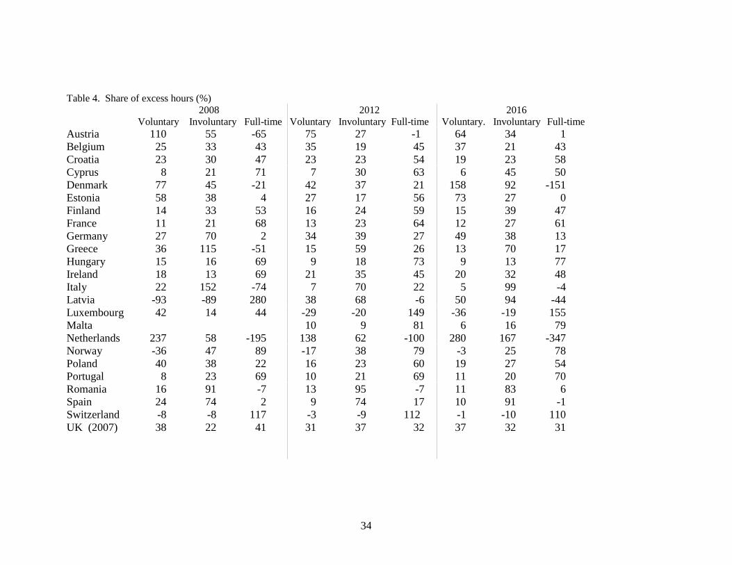
34

Table 4. Share of excess hours (%)

2008 2012 2016

Voluntary Involuntary Full-time Voluntary Involuntary Full-time Voluntary. Involuntary Full-time

Austria 110 55 -65 75 27 -1 64 34 1

Belgium 25 33 43 35 19 45 37 21 43

Croatia 23 30 47 23 23 54 19 23 58

Cyprus 8 21 71 7 30 63 6 45 50

Denmark 77 45 -21 42 37 21 158 92 -151

Estonia 58 38 4 27 17 56 73 27 0

Finland 14 33 53 16 24 59 15 39 47

France 11 21 68 13 23 64 12 27 61

Germany 27 70 2 34 39 27 49 38 13

Greece 36 115 -51 15 59 26 13 70 17

Hungary 15 16 69 9 18 73 9 13 77

Ireland 18 13 69 21 35 45 20 32 48

Italy 22 152 -74 7 70 22 5 99 -4

Latvia -93 -89 280 38 68 -6 50 94 -44

Luxembourg 42 14 44 -29 -20 149 -36 -19 155

Malta 10 9 81 6 16 79

Netherlands 237 58 -195 138 62 -100 280 167 -347

Norway -36 47 89 -17 38 79 -3 25 78

Poland 40 38 22 16 23 60 19 27 54

Portugal 8 23 69 10 21 69 11 20 70

Romania 16 91 -7 13 95 -7 11 83 6

Spain 24 74 2 9 74 17 10 91 -1

Switzerland -8 -8 117 -3 -9 112 -1 -10 110

UK (2007) 38 22 41 31 37 32 37 32 31

35

Table 5. Annual Average Wage Changes 2000-2016 (annual % changes)

Nominal Real

2000-2007 2008-2016 2000-2007. 2008-2016

Australia 4.2 2.9 1.3 0.6

Austria 2.8 2.3 0.8 0.4

Belgium 2.5 1.7 0.1 0.3

Canada 3.5 2.6 1.7 1.2

Chile 4.9 7.0 1.3 2.7

Czech Republic 6.9 2.4 4.6 1.1

Denmark 3.4 2.7 1.5 1.1

Estonia 13.2 4.2 8.1 1.4

Finland 3.4 2.4 1.8 0.5

France 3.0 1.7 1.1 1.0

Germany 1.6 2.3 0.2 1.1

Greece 5.7 -1.7 2.6 -2.2

Hungary 10.9 2.9 4.3 0.1

Iceland 7.8 5.0 3.1 0.0

Ireland 5.9 1.2 2.4 1.2

Israel 1.8 2.3 0.2 0.5

Italy 3.1 1.2 0.4 -0.1

Japan -0.8 -0.2 -0.1 0.0

Korea 5.6 2.7 2.5 0.5

Latvia 16.5 3.9 8.9 1.7

Lithuania 9.8 4.0 8.2 1.3

Luxembourg 3.8 1.8 1.4 0.7

Mexico 7.8 3.6 2.3 -0.7

Netherlands 3.5 1.8 1.0 0.7

New Zealand 4.3 2.3 2.5 0.8

Norway 4.7 3.6 2.8 1.3

Poland 4.8 3.8 1.2 2.0

Portugal 3.4 0.6 0.0 -0.4

Slovak Republic 8.9 3.2 3.6 1.7

Slovenia 8.0 2.1 3.0 0.9

Spain 3.3 1.8 -0.1 0.7

Sweden 3.5 2.7 2.2 1.3

Switzerland 1.9 0.5 -1.0 0.6

United Kingdom 4.1 1.7 2.7 -0.3

United States 3.8 2.2 1.5 0.7

Note: Average annual wages per full-time equivalent dependent employee are obtained by

dividing the national-accounts-based total wage bill by the average number of employees

in the total economy, which is then multiplied by the ratio of average usual weekly hours

per full-time employee to average usually weekly hours for all employees. Real wage

growth is in constant 2016 prices NICU For more details, see:

www.oecd.org/employment/outlook

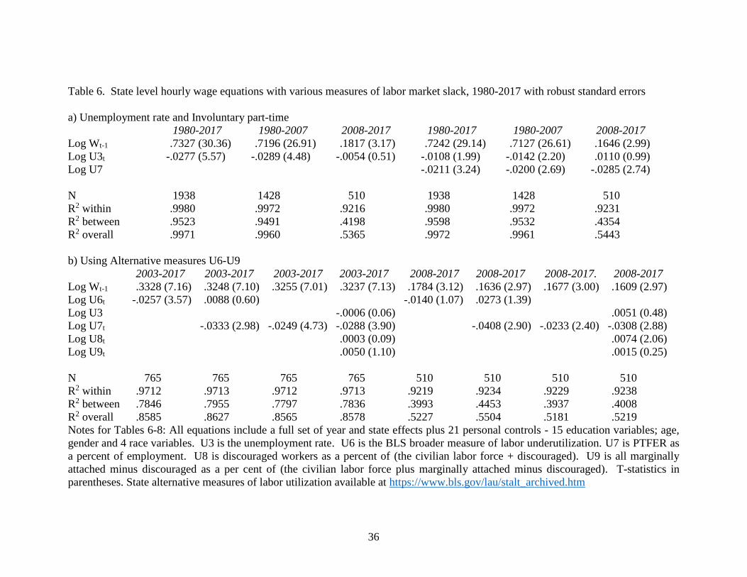
36

Table 6. State level hourly wage equations with various measures of labor market slack, 1980-2017 with robust standard errors

a) Unemployment rate and Involuntary part-time

1980-2017 1980-2007 2008-2017 1980-2017 1980-2007 2008-2017

Log Wt-1 .7327 (30.36) .7196 (26.91) .1817 (3.17) .7242 (29.14) .7127 (26.61) .1646 (2.99)

Log U3t -.0277 (5.57) -.0289 (4.48) -.0054 (0.51) -.0108 (1.99) -.0142 (2.20) .0110 (0.99)

Log U7 -.0211 (3.24) -.0200 (2.69) -.0285 (2.74)

N 1938 1428 510 1938 1428 510

R2 within .9980 .9972 .9216 .9980 .9972 .9231

R2 between .9523 .9491 .4198 .9598 .9532 .4354

R2 overall .9971 .9960 .5365 .9972 .9961 .5443

b) Using Alternative measures U6-U9

2003-2017 2003-2017 2003-2017 2003-2017 2008-2017 2008-2017 2008-2017. 2008-2017

Log Wt-1 .3328 (7.16) .3248 (7.10) .3255 (7.01) .3237 (7.13) .1784 (3.12) .1636 (2.97) .1677 (3.00) .1609 (2.97)

Log U6t -.0257 (3.57) .0088 (0.60) -.0140 (1.07) .0273 (1.39)

Log U3 -.0006 (0.06) .0051 (0.48)

Log U7t -.0333 (2.98) -.0249 (4.73) -.0288 (3.90) -.0408 (2.90) -.0233 (2.40) -.0308 (2.88)

Log U8t .0003 (0.09) .0074 (2.06)

Log U9t .0050 (1.10) .0015 (0.25)

N 765 765 765 765 510 510 510 510

R2 within .9712 .9713 .9712 .9713 .9219 .9234 .9229 .9238

R2 between .7846 .7955 .7797 .7836 .3993 .4453 .3937 .4008

R2 overall .8585 .8627 .8565 .8578 .5227 .5504 .5181 .5219

Notes for Tables 6-8: All equations include a full set of year and state effects plus 21 personal controls - 15 education variables; age,

gender and 4 race variables. U3 is the unemployment rate. U6 is the BLS broader measure of labor underutilization. U7 is PTFER as

a percent of employment. U8 is discouraged workers as a percent of (the civilian labor force + discouraged). U9 is all marginally

attached minus discouraged as a per cent of (the civilian labor force plus marginally attached minus discouraged). T-statistics in

parentheses. State alternative measures of labor utilization available at https://www.bls.gov/lau/stalt_archived.htm

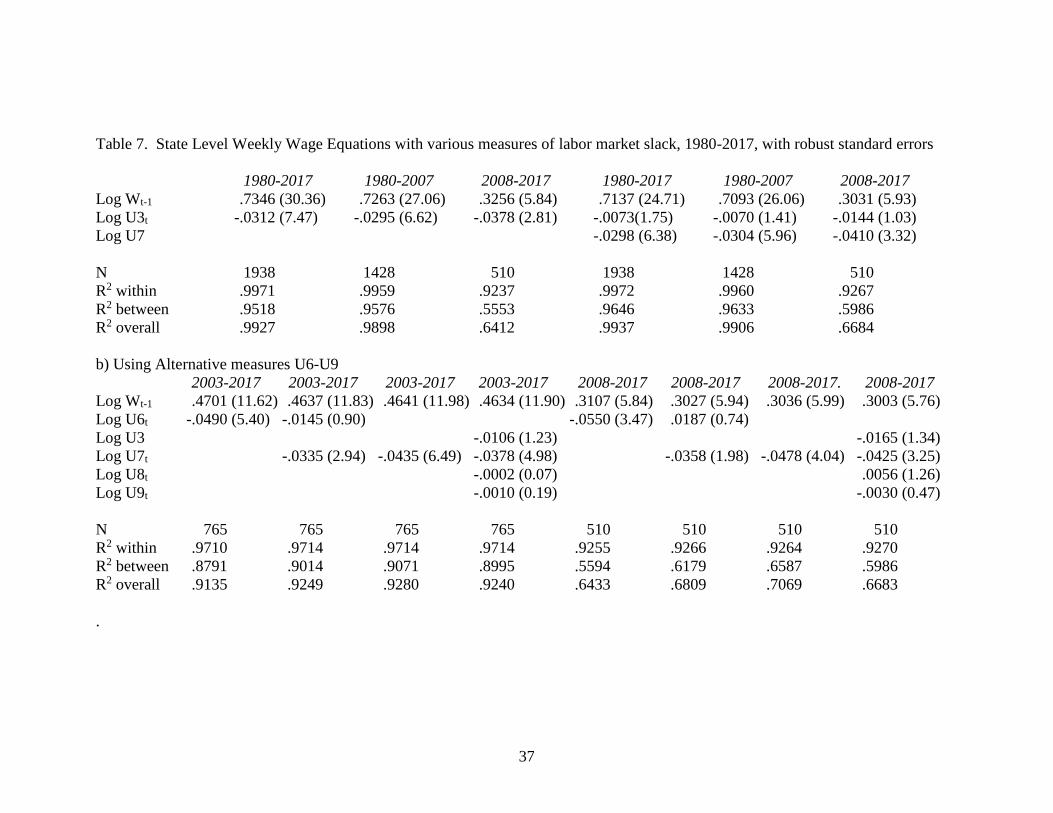
37

Table 7. State Level Weekly Wage Equations with various measures of labor market slack, 1980-2017, with robust standard errors

1980-2017 1980-2007 2008-2017 1980-2017 1980-2007 2008-2017

Log Wt-1 .7346 (30.36) .7263 (27.06) .3256 (5.84) .7137 (24.71) .7093 (26.06) .3031 (5.93)

Log U3t -.0312 (7.47) -.0295 (6.62) -.0378 (2.81) -.0073(1.75) -.0070 (1.41) -.0144 (1.03)

Log U7 -.0298 (6.38) -.0304 (5.96) -.0410 (3.32)

N 1938 1428 510 1938 1428 510

R2 within .9971 .9959 .9237 .9972 .9960 .9267

R2 between .9518 .9576 .5553 .9646 .9633 .5986

R2 overall .9927 .9898 .6412 .9937 .9906 .6684

b) Using Alternative measures U6-U9

2003-2017 2003-2017 2003-2017 2003-2017 2008-2017 2008-2017 2008-2017. 2008-2017

Log Wt-1 .4701 (11.62) .4637 (11.83) .4641 (11.98) .4634 (11.90) .3107 (5.84) .3027 (5.94) .3036 (5.99) .3003 (5.76)

Log U6t -.0490 (5.40) -.0145 (0.90) -.0550 (3.47) .0187 (0.74)

Log U3 -.0106 (1.23) -.0165 (1.34)

Log U7t -.0335 (2.94) -.0435 (6.49) -.0378 (4.98) -.0358 (1.98) -.0478 (4.04) -.0425 (3.25)

Log U8t -.0002 (0.07) .0056 (1.26)

Log U9t -.0010 (0.19) -.0030 (0.47)

N 765 765 765 765 510 510 510 510

R2 within .9710 .9714 .9714 .9714 .9255 .9266 .9264 .9270

R2 between .8791 .9014 .9071 .8995 .5594 .6179 .6587 .5986

R2 overall .9135 .9249 .9280 .9240 .6433 .6809 .7069 .6683

.

38

Table 8. Wages and change in the home ownership rate, with robust standard errors

a) Hourly

1980-2017 1980-2017 1980-2007 1980-2007 2008-2017 2008-2017

Log Wt-1 .6893 (26.43) .6880 (25.97) .6761 (23.51) .6743 (23.03) .1617 (2.92) .1656 (2.94)

Log U7t -.0219 (3.06) -.0264 (4.66) -.0193 (2.19) -.0251 (3.20) -.0388 (2.79) -.0218 (2.30)

Log U3t -.0087 (1.37) -.0119 (1.59)

Log U6t .0264 (1.36)

Log Homet Log Homet-1 .0604 (1.57) .0613 (1.59) .0231 (0.45) .0248 (0.48) .1349 (3.08) .1368 (3.16)

N 1683 1683 1173 1173 510 510

R2 within .9974 .9974 .9965 .9965 .9244 .9240

R2 between .9414 .9492 .9183 .9291 .4156 .3667

R2 overall .9957 .9959 .9941 .9944 .5313 .4999

b) Weekly

1980-2017 1980-2017 1980-2007 1980-2007 2008-2017 2008-2017

Log Wt-1 .6485 (17.13) .6467 (17.15) .6028 (12.91) .6025 (13.31) .3099 (6.09) .3107 (6.15)

Log U7t -.0219 (3.06) -.0317 (6.84) -.0264 (4.71) -.0266 (5.39) -.0329 (1.83) -.0218 (2.30)

Log U3t -.0087 (1.37) -.0005 (0.09)

Log U6t -.0200 (0.79)

Log Homet Log Homet-1 .0604 (1.57) .1279 (3.61) .0231 (0.45) .0991 (2.41) .1349 (3.08) .1728 (3.01)

N 1683 1683 1173 1173 510 510

R2 within .9961 .9960 .9939 .9939 .9282 .9280

R2 between .9583 .9610 .9508 .9510 .6045 .6485

R2 overall .9894 .9897 .9812 .9812 .6722 .7005

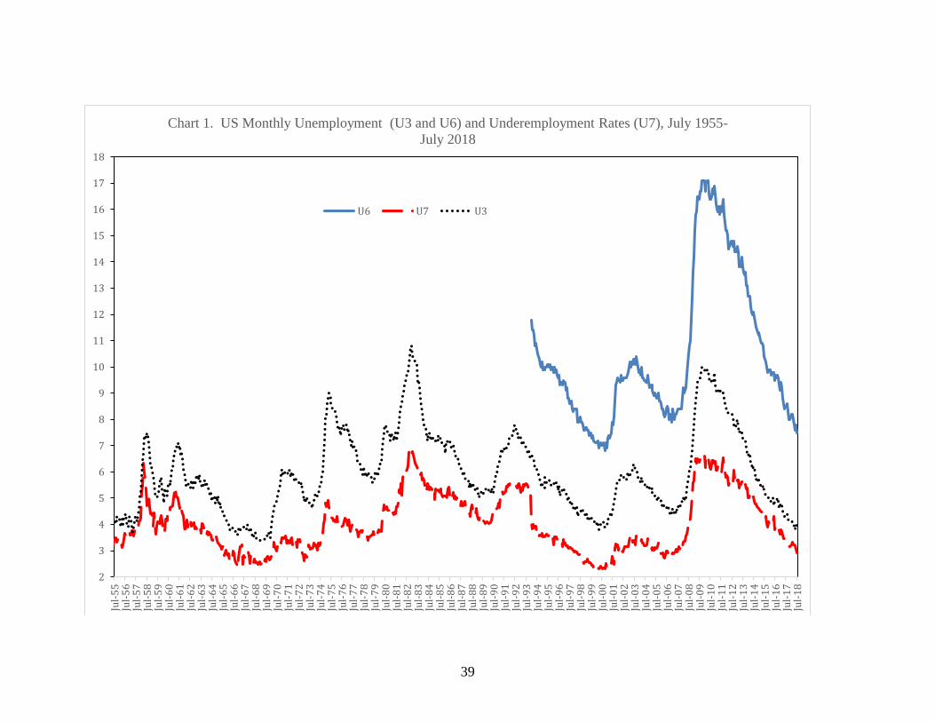
39

2

3

4

5

6

7

8

9

10

11

12

13

14

15

16

17

18

Jul-

55

Jul-

56

Jul-

57

Jul-

58

Jul-

59

Jul-

60

Jul-

61

Jul-

62

Jul-

63

Jul-

64

Jul-

65

Jul-

66

Jul-

67

Jul-

68

Jul-

69

Jul-

70

Jul-

71

Jul-

72

Jul-

73

Jul-

74

Jul-

75

Jul-

76

Jul-

77

Jul-

78

Jul-

79

Jul-

80

Jul-

81

Jul-

82

Jul-

83

Jul-

84

Jul-

85

Jul-

86

Jul-

87

Jul-

88

Jul-

89

Jul-

90

Jul-

91

Jul-

92

Jul-

93

Jul-

94

Jul-

95

Jul-

96

Jul-

97

Jul-

98

Jul-

99

Jul-

00

Jul-

01

Jul-

02

Jul-

03

Jul-

04

Jul-

05

Jul-

06

Jul-

07

Jul-

08

Jul-

09

Jul-

10

Jul-

11

Jul-

12

Jul-

13

Jul-

14

Jul-

15

Jul-

16

Jul-

17

Jul-

18

Chart 1. US Monthly Unemployment (U3 and U6) and Underemployment Rates (U7), July 1955-

July 2018

U6 U7 U3

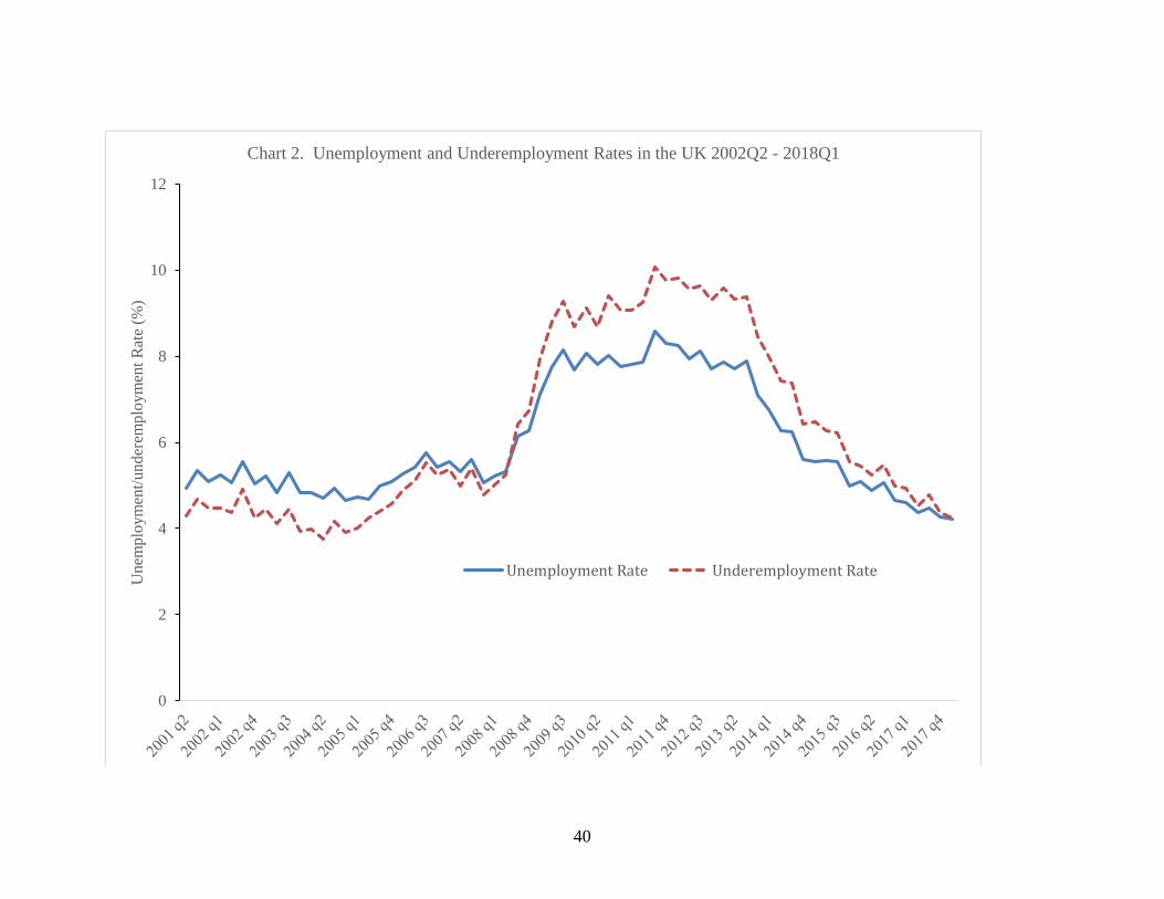
40

0

2

4

6

8

10

12

Un

emp

loym

ent/

under

emplo

ym

ent

Rat

e (%

)Chart 2. Unemployment and Underemployment Rates in the UK 2002Q2 - 2018Q1

Unemployment Rate Underemployment Rate

41

0

5

10

15

20

25

30

35

40

45

50

More

Hours

/Few

er H

ours

(m

illi

ons

per

wee

kChart 3. More and Fewer Desired Hours in the UK 2001Q2 - 2018Q1

More Hours Fewer Hours

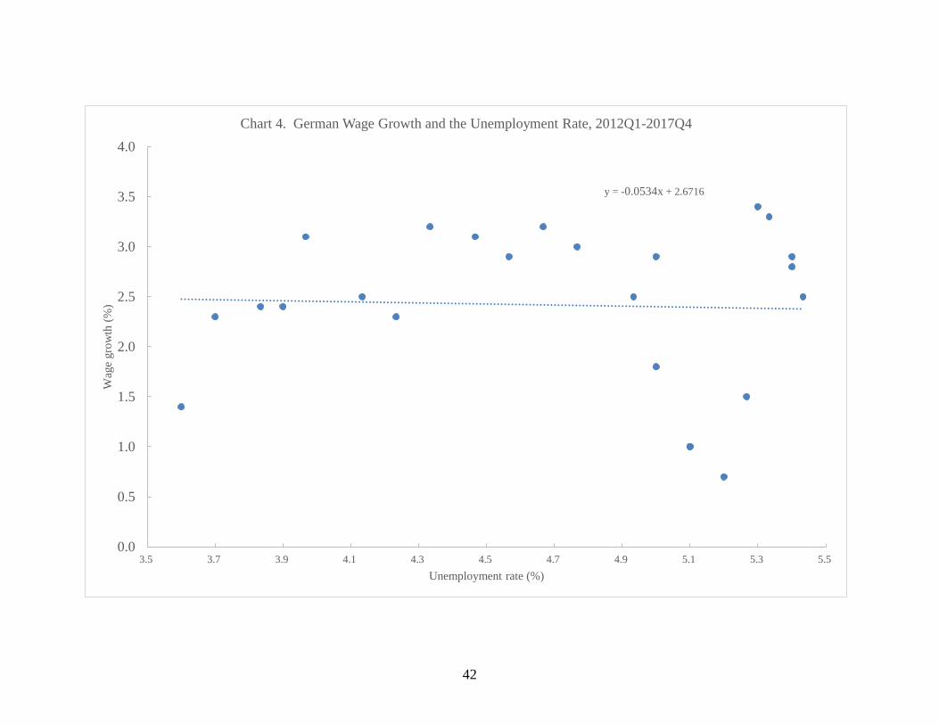
42

y = -0.0534x + 2.6716

0.0

0.5

1.0

1.5

2.0

2.5

3.0

3.5

4.0

3.5 3.7 3.9 4.1 4.3 4.5 4.7 4.9 5.1 5.3 5.5

Wag

e gro

wth

(%

)

Unemployment rate (%)

Chart 4. German Wage Growth and the Unemployment Rate, 2012Q1-2017Q4

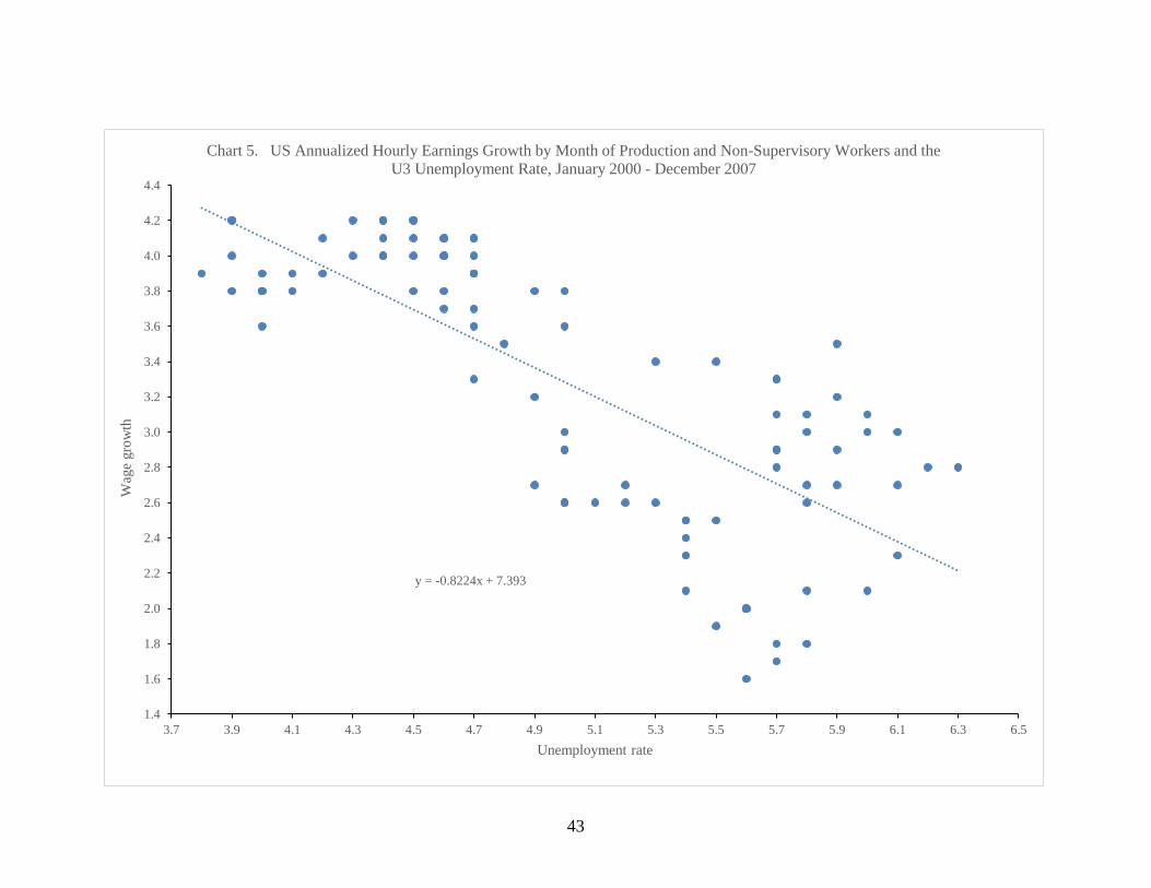
43

y = -0.8224x + 7.393

1.4

1.6

1.8

2.0

2.2

2.4

2.6

2.8

3.0

3.2

3.4

3.6

3.8

4.0

4.2

4.4

3.7 3.9 4.1 4.3 4.5 4.7 4.9 5.1 5.3 5.5 5.7 5.9 6.1 6.3 6.5

Wag

e gro

wth

Unemployment rate

Chart 5. US Annualized Hourly Earnings Growth by Month of Production and Non-Supervisory Workers and the

U3 Unemployment Rate, January 2000 - December 2007

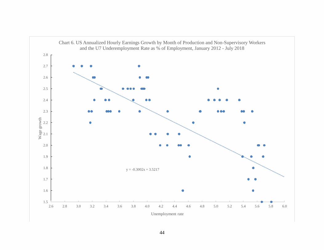
44

y = -0.3002x + 3.5217

1.5

1.6

1.7

1.8

1.9

2.0

2.1

2.2

2.3

2.4

2.5

2.6

2.7

2.8

2.6 2.8 3.0 3.2 3.4 3.6 3.8 4.0 4.2 4.4 4.6 4.8 5.0 5.2 5.4 5.6 5.8 6.0

Wag

e gro

wth

Unemployment rate

Chart 6. US Annualized Hourly Earnings Growth by Month of Production and Non-Supervisory Workers

and the U7 Underemployment Rate as % of Employment, January 2012 - July 2018