Embed Size (px)
Citation preview
Dave Lage Moderno Shadow Mapping and Ray-Tracing
Tese de Mestrado Mestrado em Informática Trabalho efectuado sob a orientação doProfessor Doutor António Ramires Fernandes
Setembro 2011
Tracing
orientação do Professor Doutor António Ramires Fernandes

É AUTORIZADA A REPRODUÇÃO INTEGRAL DESTA TESE APENAS PARA EFEITOS DE INVESTIGAÇÃO, MEDIANTE DECLARAÇÃO ESCRITA DO INTERESSADO, QUE A TAL SE COMPROMETE.
Universidade do Minho, ___/___/______
Assinatura: ________________________________________________

iii
ACKNOWLEDGMENTS
I would like to thank the following people:
- my family, and especially my parents Celeste and Albino for sponsoring this work
(and my life in general);
- my friends, too many to be named here, be it those with whom I studied, those with
whom I played (and still play) videogames or those with whom I just hang out with;
- my thesis advisor, PhD António Ramires Fernandes, for putting up with all of my
questions (many of which weren’t very smart);
- my girlfriend, Helena, for supporting me in finishing this work, even considering all
the time it took to finish.

iv
v
SHADOW MAPPING AND RAY-TRACING
ABSTRACT
Shadow mapping has been one of the most used algorithms for real time calculation of shadows, since
it is extremely simple and quick in calculating said shadows, but not always presents the best results.
On the other hand, ray-tracing presents pixel-perfect shadows, but it is more demanding from a
computational point of view.
Shadow mapping has seen many proposals to increase its accuracy, while retaining its high
performance nature. Some of the methods proposed, based solely on the standard shadow mapping
technique, do improve significantly the standard shadow mapping result at the expense of a minor
decrease in performance. Other approaches propose hybrid methods, using shadow mapping as a way
of limiting the number of pixels that require ray-tracing. One of such approaches uses texel coherence
to reduce the number of pixels that require testing.
These latter approaches establish the theme for this work. The goal is to narrow down as much as
possible the amount of pixels that require a ray-tracer to determine its shadow status.
The first step was to identify the location of the errors present in a shadow map. The tests confirmed
the intuition that most of these errors should be located in the contours of the shadow areas.
The next step focuses on these contour areas and looks for ways to determine the correctness of a
pixel’s shadow status. Several methods were proposed to achieve this goal. Some methods were
capable of confirming pixels in shadow. Some were capable of correcting pixels in light.
Each method, with the exception of texel coherence, uses a very selective ray-tracer, i.e. only very
few triangles are tested for intersection with a single light ray.
Since each method has its strengths and weaknesses an algorithm was proposed, chaining all these
methods together. The first step is to determine the set of pixels in the contours of the shadow areas.
Then each method is applied in turn, so that only the pixels the remaining unconfirmed/uncorrected
pass on to the next stage.
At the end of the algorithm a very large percentage of pixels in shadow were confirmed and a
significant number of pixels in light were corrected. The remaining pixels could then be fed to a full
ray-tracer. The load of the ray-tracer is severely reduced under this approach making it an affordable
solution to obtain pixel perfect shadows in the contours of the shadowed areas.

vi
vii
SHADOW MAPPING E RAY-TRACING
RESUMO
O shadow mapping tem sido um dos algoritmos mais utilizados para o cálculo de sombras em tempo
real, já que é extremamente simples e rápido em calcular estas sombras, mas nem sempre apresenta os
melhores resultados. Por outro lado, ray-tracing apresenta sombras perfeitas ao nível do pixel mas é
mais exigente de um ponto de vista computacional.
Têm havido muitas propostas para o aumento de qualidade do shadow mapping sem afectar o seu
desempenho. Alguns dos métodos propostos, baseados somente na técnica de shadow mapping
padrão, de facto melhoram significativamente o resultado do shadow mapping padrão ao custo de uma
pequena diminuição no desempenho. Outras abordagens propõem métodos híbridos, usando o shadow
mapping para limitar o número de pixéis que requerem ray-tracing. Uma destas abordagens usa o
texel coherence para reduzir o número de pixéis que precisam de ser testados.
Estas últimas abordagens estabelecem o tema deste trabalho. O objectivo é limitar o máximo possível
a quantidade de pixéis que requerem um ray-tracer para determinar o seu sombreamento.
O primeiro passo foi identificar a localização dos erros presentes num shadow map. Os testes
confirmaram a intuição de que a maior parte destes erros se deveriam encontrar nos contornos das
zonas sombreadas.
O próximo passo foca-se nestas áreas de contorno e procura maneiras de determinar se o
sombreamento de um pixel está correcto. Vários métodos foram propostos para conseguir este
objectivo. Alguns métodos foram capazes de confirmar pixéis em sombra. Alguns foram capazes de
corrigir pixéis em luz.
Cada método, com a excepção do texel coherence, usa um ray-tracer muito selectivo, isto é, apenas
uma muito pequena quantidade de triângulos é testada para intersecção com cada raio de luz.
Como cada método tem as suas vantagens e desvantagens um algoritmo que encadeia todos estes
métodos foi proposto. O primeiro passo é determinar o conjunto de pixéis nos contornos das áreas
sombreadas. Depois cada método é aplicado à vez de modo a que os pixéis que se mantêm por
confirmar ou corrigir passem para o próximo passo.
No fim do algoritmo uma grande percentagem de pixéis em sombra foi confirmada e um número
significativo de pixéis em luz foi corrigido. O resto dos pixéis poderia então passar por um ray-tracer
completo. A carga do ray-tracer é severamente reduzida sob esta abordagem tornando-o numa
solução acessível à obtenção de sombras perfeitas ao nível do pixel nos contornos das áreas
sombreadas.

viii

ix
TABLE OF CONTENTS
1. INTRODUCTION ............................................................................... 1
1.1. Motivation ................................................................................................................... 2
1.2. Goals............................................................................................................................ 2
1.3. Methodology ............................................................................................................... 3
1.4. Thesis Structure ........................................................................................................... 4
2. STATE OF THE ART ......................................................................... 5
2.1. Shadow Mapping......................................................................................................... 5
2.1.1. Shadow Mapping Basics .................................................................................................. 5
2.1.2. Shadow Mapping Problems ............................................................................................ 6
2.1.3. Shadow Mapping Approaches ........................................................................................ 8
2.2. Ray-Tracing ............................................................................................................... 13
2.2.1. Ray-Tracing Basics ......................................................................................................... 13
2.3. Combining Both ........................................................................................................ 15
2.3.1. Coherence-Based Ray-Tracing ...................................................................................... 15
2.3.2. Hybrid GPU Rendering Pipeline for Alias-Free Hard Shadows ...................................... 16
2.3.3. Hybrid GPU-CPU Renderer ............................................................................................ 18
2.4. Conclusion ................................................................................................................. 19
3. ALGORITHM DESCRIPTION ........................................................ 21
3.1. Shadow Mapping Errors............................................................................................ 21
3.1.1. Shadow Status and Errors ............................................................................................. 21
3.1.2. Error Location ................................................................................................................ 23
3.2. Using Texel Information ........................................................................................... 24
3.3. Using the Information of the Neighbouring Texels .................................................. 28
3.4. Using Texel Coherence ............................................................................................. 31
3.5. Using Geometric Adjacency Information ................................................................. 34
x
3.6. Putting It All Together .............................................................................................. 37
3.7. Conclusion ................................................................................................................. 41
4. ALGORITHM TESTING .................................................................. 43
4.1. Test Scenes ................................................................................................................ 44
4.2. Ray-Tracer ................................................................................................................. 46
4.3. Shadow Mapping Errors............................................................................................ 52
4.4. Using Texel Coherence ............................................................................................. 55
4.5. Using Texel Information ........................................................................................... 60
4.6. Using the Information of the Neighbours of the Texel ............................................. 63
4.7. Using Geometric Adjacency Information ................................................................. 67
4.8. Putting It All Together .............................................................................................. 71
4.9. Final Observations..................................................................................................... 76
5. CONCLUSIONS AND FUTURE WORK ........................................ 81
6. BIBLIOGRAPHY ............................................................................. 85
APPENDIX ............................................................................................... 87
xi
FIGURE INDEX
Figure 1: How a Shadow Map works. ....................................................................................... 6
Figure 2: The shadow of the tree presents aliasing. ................................................................... 6
Figure 3: Perspective Shadow Map example. ............................................................................ 8
Figure 4: Light Space Perspective Shadow Map example. ........................................................ 9
Figure 5: Trapezoidal Shadow Mapping movement flickering. .............................................. 10
Figure 6: Adaptive Shadow map result compared to a shadow mapping result (2048x2048
shadow map versus an effective 524288x524288 shadow map result). .................................. 10
Figure 7: Parallel-Split Shadow Maps example....................................................................... 11
Figure 8: Variance Shadow Map light leaking example. ......................................................... 12
Figure 9: Comparison between Convoluted, Variance and Exponential Shadow Maps
respectively. ............................................................................................................................. 12
Figure 10: Simple example of Ray-Tracing............................................................................. 14
Figure 11: Reference image examples for the coherence based ray-tracing. .......................... 16
Figure 12: Resizing the triangle by moving its edges. ............................................................. 17
Figure 13: Example of the uncertain areas when using the Hybrid GPU Rendering Pipeline
for Alias-Free Hard Shadows................................................................................................... 18
Figure 14: Green pixels mark where shadow mapping samples disagree in the Hybrid GPU-
CPU Renderer. ......................................................................................................................... 19
Figure 15: Correctly (in green) and incorrectly (in blue) shadowed points by shadow
mapping.................................................................................................................................... 22
Figure 16: Correctly (in green) and incorrectly (in blue) lit points by shadow mapping. ....... 23
Figure 17: Marked contours and errors of the scene. ............................................................... 24
Figure 18: Cases of using texel information. ........................................................................... 25
Figure 19: Correcting a point wrongly defined in light with the triangle stored in the projected
texel. ......................................................................................................................................... 26
xii
Figure 20: Pixel confirmation using texel information. ........................................................... 27
Figure 21: The two cases of neighbouring texels. ................................................................... 28
Figure 22: Cases using neighbouring texel information with a triangle stored in the centre
texel. ......................................................................................................................................... 29
Figure 23: Cases using neighbouring texel information without a triangle stored in the centre
texel. ......................................................................................................................................... 30
Figure 24: Pixel confirmation using neighbouring texel information with 8 neighbours. ....... 31
Figure 25: Examples of PCF results. ....................................................................................... 32
Figure 26: Pixel confirmation using PCF with four texels. ..................................................... 33
Figure 27: Using adjacent geometry information for case a). ................................................. 35
Figure 28: Using adjacent geometry information for case b). ................................................. 35
Figure 29: Correcting a point wrongly defined in light using triangle adjacency. .................. 36
Figure 30: Pixel confirmation using geometry adjacency information with 2 levels of
adjacency.................................................................................................................................. 37
Figure 31: Average of corrected/confirmed/hinted contour pixels by each method: a) contour
pixels; b) shadow map results separated in shadow (black) and light (white); c) errors of the
shadow map (gray); d) correct (blue) and incorrect (red) hints using texel coherence; e)
confirmed shadow (dark green) and corrected light (light green) pixels by neighbouring
texels; f) confirmed shadow pixels (orange) by adjacent geometry. ....................................... 38
Figure 32: Average of corrected/confirmed/hinted contour pixels by the chaining of methods:
a) contour pixels; b) shadow map results separated in shadow (black) and light (white); c)
errors of the shadow map (gray); d) correct (blue) and incorrect (red) hints using texel
coherence; e) confirmed shadow (dark green) and corrected light (light green) pixels by
neighbouring texels; f) confirmed shadow pixels (orange) by adjacent geometry; g) non-
hinted/uncorrected/unconfirmed pixels (yellow). .................................................................... 40
Figure 33: The side (left), with (centre) and against (right) viewpoints of the first scene. ..... 44
Figure 34: The side (left), with (centre) and against (right) viewpoints of the second scene. . 45
xiii
Figure 35: The with (left), side (centre) and against (right) viewpoints of the third scene. .... 46
Figure 36: The side (left), against (centre) and with (right) viewpoints of the fourth scene. .. 46
Figure 37: Ray-tracer results for the side viewpoint of the primitives scene. ......................... 47
Figure 38: Ray-tracer results for the with viewpoint of the primitives scene. ......................... 47
Figure 39: Ray-tracer results for the against viewpoint of the primitives scene. .................... 48
Figure 40: Ray-tracer results for the side viewpoint of the bench scene. ................................ 48
Figure 41: Ray-tracer results for the with viewpoint of the bench scene. ............................... 49
Figure 42: Ray-tracer results for the against viewpoint of the bench scene. ........................... 49
Figure 43: Ray-tracer results for the with viewpoint of the trees scene. ................................. 50
Figure 44: Ray-tracer results for the side viewpoint of the trees scene. .................................. 50
Figure 45: Ray-tracer results for the against viewpoint of the trees scene. ............................. 51
Figure 46: Ray-tracer results for the side viewpoint of the flowers scene. .............................. 51
Figure 47: Ray-tracer results for the against viewpoint of the flowers scene. ......................... 52
Figure 48: Ray-tracer results for the with viewpoint of the flowers scene. ............................. 52
Figure 49: Best case of shadow map errors being caught inside contours with a 2048x2048
shadow map. ............................................................................................................................ 53
Figure 50: Worst case of shadow map errors being caught inside contours with a 2048x2048
shadow map. ............................................................................................................................ 54
Figure 51: Average case of shadow map errors being caught inside contours. ....................... 54
Figure 52: Average shadow map results separated by contour thickness with a 1024x1024
shadow map (top) and a 2048x2048 shadow map (bottom). ................................................... 55
Figure 53: Best case of texel coherence confirmation using four texels and a 2048x2048
shadow map. ............................................................................................................................ 56
Figure 54: Worst case of texel coherence confirmation using four texels and a 2048x2048
shadow map. ............................................................................................................................ 57
xiv
Figure 55: Average case of texel coherence confirmation using four texels. .......................... 58
Figure 56: Best case of texel coherence confirmation using nine texels and a 2048x2048
shadow map. ............................................................................................................................ 59
Figure 57: Worst case of texel coherence confirmation using nine texels and a 2048x2048
shadow map. ............................................................................................................................ 59
Figure 58: Average case of texel coherence confirmation using nine texels. .......................... 60
Figure 59: Average results of texel coherence with four texels separated by contour thickness
with a 1024x1024 shadow map (top) and a 2048x2048 shadow map (bottom). ..................... 60
Figure 60: Best case of only using centre texel information with a 2048x2048 shadow map. 61
Figure 61: Worst case of using centre texel information by itself with a 2048x2048 shadow
map. .......................................................................................................................................... 62
Figure 62: Average case of using centre texel information by itself. ...................................... 62
Figure 63: Best case of only using information of four neighbouring texels with a 2048x2048
shadow map. ............................................................................................................................ 64
Figure 64: Best case of only using information of nine neighbouring texels with a 2048x2048
shadow map. ............................................................................................................................ 64
Figure 65: Worst case of only using information of four neighbouring texels with a
2048x2048 shadow map. ......................................................................................................... 65
Figure 66: Worst case of only information of nine neighbouring texels with a 2048x2048
shadow map. ............................................................................................................................ 65
Figure 67: Average case of only using information of four neighbouring texels. ................... 66
Figure 68: Average case of only using information of nine neighbouring texels. ................... 66
Figure 69: Average results of neighbouring texels with nine texels separated by contour
thickness with a 1024x1024 shadow map (top) and a 2048x2048 shadow map (bottom). ..... 67
Figure 70: Best case of only using centre and first level of adjacent geometry information
with a 2048x2048 shadow map................................................................................................ 68
xv
Figure 71: Best case of only using centre and second level of adjacent geometry information
with a 2048x2048 shadow map................................................................................................ 68
Figure 72: Worst case of only using centre and first level of adjacent geometry information
with a 2048x2048 shadow map................................................................................................ 69
Figure 73: Worst case of only using centre and second level of adjacent geometry information
with a 2048x2048 shadow map................................................................................................ 69
Figure 74: Average case of only using centre and first level of adjacent geometry
information. .............................................................................................................................. 70
Figure 75: Average case of only using centre and second level of adjacent geometry
information. .............................................................................................................................. 70
Figure 76: Average results of adjacent geometry with two levels of adjacency separated by
contour thickness with a 1024x1024 shadow map (top) and a 2048x2048 shadow map
(bottom).................................................................................................................................... 71
Figure 77: Best case of algorithm pixel confirmation after using information of the
neighbouring texels with a 2048x2048 shadow map. .............................................................. 72
Figure 78: Worst case of algorithm pixel confirmation after using information of the
neighbouring texels with a 2048x2048 shadow map. .............................................................. 72
Figure 79: Average case of algorithm pixel confirmation after using information of the
neighbouring texels. ................................................................................................................. 73
Figure 80: Average results of the algorithm after the neighbouring texel step separated by
contour thickness with a 1024x1024 shadow map (top) and a 2048x2048 shadow map
(bottom).................................................................................................................................... 73
Figure 81: Best case of algorithm pixel confirmation after using information of the adjacent
geometry with a 2048x2048 shadow map. .............................................................................. 74
Figure 82: Worst case of algorithm pixel confirmation after using information of the adjacent
geometry with a 2048x2048 shadow map. .............................................................................. 75
Figure 83: Average case of algorithm pixel confirmation after using information of the
adjacent geometry. ................................................................................................................... 75
xvi
Figure 84: Average results of the algorithm after the adjacent geometry step separated by
contour thickness with a 1024x1024 shadow map (top) and a 2048x2048 shadow map
(bottom).................................................................................................................................... 76
Figure 85: Average results of the algorithm after the adjacent geometry step with pixels that
were not confirmed, corrected or hinted marked, separated by contour thickness with a
1024x1024 shadow map (top) and a 2048x2048 shadow map (bottom). ................................ 76
Figure 86: Marked errors of the best case when using a 2048x2048 shadow map. ................ 78
Figure 87: Marked errors of the worst case when using a 2048x2048 shadow map. .............. 78
Figure 88: Marked errors of the average case. ......................................................................... 79
Figure 89: Result of the ray-tracing approach for the side viewpoint of the primitives scene.
.................................................................................................................................................. 87
Figure 90: Result of the shadow mapping approach for the side viewpoint of the primitives
scene. ........................................................................................................................................ 87
Figure 91: Result of texel coherence with four texels for the side viewpoint of the primitives
scene. ........................................................................................................................................ 88
Figure 92: Result of texel coherence with nine texels for the side viewpoint of the primitives
scene. ........................................................................................................................................ 88
Figure 93: Result of the single texel approach on the side viewpoint of the primitives scene.
.................................................................................................................................................. 89
Figure 94: Result of the neighbour texels approach using four neighbours for the side
viewpoint of the primitives scene. ........................................................................................... 89
Figure 95: Result of the neighbour texels approach using nine neighbours for the side
viewpoint of the primitives scene. ........................................................................................... 90
Figure 96: Result of the adjacent geometry approach with one level of adjacency for the side
viewpoint of the primitives scene. ........................................................................................... 90
Figure 97: Result of the adjacent geometry approach with two levels of adjacency for the side
viewpoint of the primitives scene. ........................................................................................... 91
xvii
Figure 98: Result of the algorithm with a six pixel thick contour and a 2048x2048 resolution
shadow map for the side viewpoint of the primitives scene. ................................................... 91
Figure 99: Corrected/confirmed/hinted contour pixels by each method for the side viewpoint
of the primitives scene using a 1024x1024 (top) and a 2048x2048 (bottom) resolution shadow
map. .......................................................................................................................................... 92
Figure 100: Corrected/confirmed/hinted contour pixels by the chaining of methods for the
side viewpoint of the primitives scene using a 1024x1024 (top) and a 2048x2048 (bottom)
resolution shadow map. ........................................................................................................... 93
Figure 101: Result of the ray-tracing approach for the with viewpoint of the primitives scene.
................................................................................................................................................ 104
Figure 102: Result of the shadow mapping approach for the with viewpoint of the primitives
scene. ...................................................................................................................................... 104
Figure 103: Result of texel coherence with four texels for the with viewpoint of the primitives
scene. ...................................................................................................................................... 105
Figure 104: Result of texel coherence with nine texels for the with viewpoint of the
primitives scene. .................................................................................................................... 105
Figure 105: Result of the single texel approach for the with viewpoint of the primitives scene.
................................................................................................................................................ 106
Figure 106: Result of the neighbour texels approach using four neighbours for the with
viewpoint of the primitives scene. ......................................................................................... 106
Figure 107: Result of the neighbour texels approach using nine neighbours for the with
viewpoint of the primitives scene. ......................................................................................... 107
Figure 108: Result of the adjacent geometry approach with one level of adjacency for the
with viewpoint of the primitives scene. ................................................................................. 107
Figure 109: Result of the adjacent geometry approach with two levels of adjacency for the
with viewpoint of the primitives scene. ................................................................................. 108
Figure 110: Result of the algorithm with a six pixel thick contour and a 2048x2048 resolution
shadow map for the with viewpoint of the primitives scene. ................................................ 108

xviii
Figure 111: Corrected/confirmed/hinted contour pixels by each method for the with
viewpoint of the primitives scene using a 1024x1024 (top) and a 2048x2048 (bottom)
resolution shadow map. ......................................................................................................... 109
Figure 112: Corrected/confirmed/hinted contour pixels by the chaining of methods for the
with viewpoint of the primitives scene using a 1024x1024 (top) and a 2048x2048 (bottom)
resolution shadow map. ......................................................................................................... 110
Figure 113: Result of the ray-tracing approach for the against viewpoint of the primitives
scene. ...................................................................................................................................... 120
Figure 114: Result of the shadow mapping approach for the against viewpoint of the
primitives scene. .................................................................................................................... 120
Figure 115: Result of texel coherence with four texels for the against viewpoint of the
primitives scene. .................................................................................................................... 121
Figure 116: Result of texel coherence with nine texels for the against viewpoint of the
primitives scene. .................................................................................................................... 121
Figure 117: Result of the single texel approach for the against viewpoint of the primitives
scene. ...................................................................................................................................... 122
Figure 118: Result of the neighbour texels approach using three pixels for the against
viewpoint of the primitives scene. ......................................................................................... 122
Figure 119: Result of the neighbour texels approach using eight pixels for the against
viewpoint of the primitives scene. ......................................................................................... 123
Figure 120: Result of the adjacent geometry approach with one level of adjacency for the
against viewpoint of the primitives scene. ............................................................................. 123
Figure 121: Result of the adjacent geometry approach with two levels of adjacency for the
against viewpoint of the primitives scene. ............................................................................. 124
Figure 122: Result of the algorithm with a six pixel thick contour and a 2048x2048 resolution
shadow map for the against viewpoint of the primitives scene. ............................................ 124
xix
Figure 123: Corrected/confirmed/hinted contour pixels by each method for the against
viewpoint of the primitives scene using a 1024x1024 (top) and a 2048x2048 (bottom)
resolution shadow map. ......................................................................................................... 125
Figure 124: Corrected/confirmed/hinted contour pixels by the chaining of methods for the
against viewpoint of the primitives scene using a 1024x1024 (top) and a 2048x2048 (bottom)
resolution shadow map. ......................................................................................................... 126
Figure 125: Result of the ray-tracing approach for the side viewpoint of the bench scene. .. 136
Figure 126: Result of the shadow mapping approach for the side viewpoint of the bench
scene. ...................................................................................................................................... 136
Figure 127: Result of texel coherence with four texels for the side viewpoint of the bench
scene. ...................................................................................................................................... 137
Figure 128: Result of texel coherence with nine texels for the side viewpoint of the bench
scene. ...................................................................................................................................... 137
Figure 129: Result of the single texel approach for the side viewpoint of the bench scene. . 138
Figure 130: Result of the neighbour texels approach with four neighbours for the side
viewpoint of the bench scene. ................................................................................................ 138
Figure 131: Result of the neighbour texels approach with nine neighbours for the side
viewpoint of the bench scene. ................................................................................................ 139
Figure 132: Result of the adjacent geometry approach with one level of adjacency for the side
viewpoint of the bench scene. ................................................................................................ 139
Figure 133: Result of the adjacent geometry approach with two levels of adjacency for the
side viewpoint of the bench scene. ........................................................................................ 140
Figure 134: Result of the algorithm with a six pixel thick contour and a 2048x2048 resolution
shadow map for the side viewpoint of the bench scene. ........................................................ 140
Figure 135: Corrected/confirmed/hinted contour pixels by each method for the side viewpoint
of the bench scene using a 1024x1024 (top) and a 2048x2048 (bottom) resolution shadow
map. ........................................................................................................................................ 141
xx
Figure 136: Corrected/confirmed/hinted contour pixels by the chaining of methods for the
side viewpoint of the bench scene using a 1024x1024 (top) and a 2048x2048 (bottom)
resolution shadow map. ......................................................................................................... 142
Figure 137: Result of the ray-tracing approach for the with viewpoint of the bench scene. . 152
Figure 138: Result of the shadow mapping approach for the with viewpoint of the bench
scene. ...................................................................................................................................... 152
Figure 139: Result of texel coherence with four texels for the with viewpoint of the bench
scene. ...................................................................................................................................... 153
Figure 140: Result of texel coherence with nine texels for the with viewpoint of the bench
scene. ...................................................................................................................................... 153
Figure 141: Result of the single texel approach for the with viewpoint of the bench scene. 154
Figure 142: Result of the neighbour texels approach with four neighbours for the with
viewpoint of the bench scene. ................................................................................................ 154
Figure 143: Result of the neighbour texels approach with nine neighbours for the with
viewpoint of the bench scene. ................................................................................................ 155
Figure 144: Result of the adjacent geometry approach with one level of adjacency for the
with viewpoint of the bench scene. ........................................................................................ 155
Figure 145: Result of the adjacent geometry approach with two levels of adjacency for the
with viewpoint of the bench scene. ........................................................................................ 156
Figure 146: Result of the algorithm with a six pixel thick contour and a 2048x2048 resolution
shadow map for the with viewpoint of the bench scene. ....................................................... 156
Figure 147: Corrected/confirmed/hinted contour pixels by each method for the with
viewpoint of the bench scene using a 1024x1024 (top) and a 2048x2048 (bottom) resolution
shadow map. .......................................................................................................................... 157
Figure 148: Corrected/confirmed/hinted contour pixels by the chaining of methods for the
with viewpoint of the bench scene using a 1024x1024 (top) and a 2048x2048 (bottom)
resolution shadow map. ......................................................................................................... 158

xxi
Figure 149: Result of the ray-tracing approach for the against viewpoint of the bench scene.
................................................................................................................................................ 168
Figure 150: Result of the shadow mapping approach for the against viewpoint of the bench
scene. ...................................................................................................................................... 168
Figure 151: Result of texel coherence with four texels for the against viewpoint of the bench
scene. ...................................................................................................................................... 169
Figure 152: Result of texel coherence with nine texels for the against viewpoint of the bench
scene. ...................................................................................................................................... 169
Figure 153: Result of the single texel approach for the against viewpoint of the bench scene.
................................................................................................................................................ 170
Figure 154: Result of the neighbour texels approach using four neighbours for the against
viewpoint of the bench scene. ................................................................................................ 170
Figure 155: Result of the neighbour texels approach using nine neighbours for the against
viewpoint of the bench scene. ................................................................................................ 171
Figure 156: Result of the adjacent geometry approach with one level of adjacency for the
against viewpoint of the bench scene..................................................................................... 171
Figure 157: Result of the adjacent geometry approach with two levels of adjacency for the
against viewpoint of the bench scene..................................................................................... 172
Figure 158: Result of the algorithm with a six pixel thick contour and a 2048x2048 resolution
shadow map for the against viewpoint of the bench scene. ................................................... 172
Figure 159: Corrected/confirmed/hinted contour pixels by each method for the against
viewpoint of the bench scene using a 1024x1024 (top) and a 2048x2048 (bottom) resolution
shadow map. .......................................................................................................................... 173
Figure 160: Corrected/confirmed/hinted contour pixels by the chaining of methods for the
against viewpoint of the bench scene using a 1024x1024 (left) and a 2048x2048 (bottom)
resolution shadow map. ......................................................................................................... 174
Figure 161: Result of the ray-tracing approach for the with viewpoint of the trees scene. ... 186
xxii
Figure 162: Result of the shadow mapping approach for the with viewpoint of the trees scene.
................................................................................................................................................ 186
Figure 163: Result of texel coherence with four texels for the with viewpoint of the trees
scene. ...................................................................................................................................... 187
Figure 164: Result of texel coherence with nine texels for the with viewpoint of the trees
scene. ...................................................................................................................................... 187
Figure 165: Result of the single texel approach for the with viewpoint of the trees scene. .. 188
Figure 166: Result of the neighbour texels approach using four neighbours for the with
viewpoint of the trees scene. .................................................................................................. 188
Figure 167: Result of the neighbour texels approach using nine neighbours for the with
viewpoint of the trees scene. .................................................................................................. 189
Figure 168: Result of the adjacent geometry approach with one level of adjacency for the
with viewpoint of the trees scene. .......................................................................................... 189
Figure 169: Result of the adjacent geometry approach with two levels of adjacency for the
with viewpoint of the trees scene. .......................................................................................... 190
Figure 170: Result of the algorithm with a six pixel thick contour and a 2048x2048 resolution
shadow map for the with viewpoint of the trees scene. ......................................................... 190
Figure 171: Corrected/confirmed/hinted contour pixels by each method for the with
viewpoint of the trees scene using a 1024x1024 (top) and a 2048x2048 (bottom) resolution
shadow map. .......................................................................................................................... 191
Figure 172: Corrected/confirmed/hinted contour pixels by the chaining of methods for the
with viewpoint of the trees scene using a 1024x1024 (top) and a 2048x2048 (bottom)
resolution shadow map. ......................................................................................................... 192
Figure 173: Result of the ray-tracing approach for the side viewpoint of the trees scene. .... 203
Figure 174: Result of the shadow mapping approach for the side viewpoint of the trees scene.
................................................................................................................................................ 203

xxiii
Figure 175: Result of texel coherence with four texels for the side viewpoint of the trees
scene. ...................................................................................................................................... 204
Figure 176: Result of texel coherence with nine texels for the side viewpoint of the trees
scene. ...................................................................................................................................... 204
Figure 177: Result of the single texel approach for the side viewpoint of the trees scene. ... 205
Figure 178: Result of the neighbour texels approach with four neighbours for the side
viewpoint of the trees scene. .................................................................................................. 205
Figure 179: Result of the neighbour texels approach with nine neighbours for the side
viewpoint of the trees scene. .................................................................................................. 206
Figure 180: Result of the adjacent geometry approach with one level of adjacency for the side
viewpoint of the trees scene. .................................................................................................. 206
Figure 181: Result of the adjacent geometry approach with two levels of adjacency for the
side viewpoint of the trees scene. .......................................................................................... 207
Figure 182: Result of the algorithm with a six pixel thick contour and a 2048x2048 resolution
shadow map for the side viewpoint of the trees scene. .......................................................... 207
Figure 183: Corrected/confirmed/hinted contour pixels by each method for the side viewpoint
of the trees scene using a 1024x1024 (top) and a 2048x2048 (bottom) resolution shadow
map. ........................................................................................................................................ 208
Figure 184: Corrected/confirmed/hinted contour pixels by the chaining of methods for the
side viewpoint of the trees scene using a 1024x1024 (top) and a 2048x2048 (bottom)
resolution shadow map. ......................................................................................................... 209
Figure 185: Result of the ray-tracing approach for the against viewpoint of the trees scene.
................................................................................................................................................ 219
Figure 186: Result of the shadow mapping approach for the against viewpoint of the trees
scene. ...................................................................................................................................... 219
Figure 187: Result of texel coherence with four texels for the against viewpoint of the trees
scene. ...................................................................................................................................... 220
xxiv
Figure 188: Result of texel coherence with nine texels for the against viewpoint of the trees
scene. ...................................................................................................................................... 220
Figure 189: Result of the single texel approach for the against viewpoint of the trees scene.
................................................................................................................................................ 221
Figure 190: Result of the neighbour texels approach using four neighbours for the against
viewpoint of the trees scene. .................................................................................................. 221
Figure 191: Result of the neighbour texels approach using nine neighbours for the against
viewpoint of the trees scene. .................................................................................................. 222
Figure 192: Result of the adjacent geometry approach with one level of adjacency for the
against viewpoint of the trees scene....................................................................................... 222
Figure 193: Result of the adjacent geometry approach with two level of adjacency for the
against viewpoint of the trees scene....................................................................................... 223
Figure 194: Result of the algorithm with a six pixel thick contour and a 2048x2048 resolution
shadow map for the against viewpoint of the trees scene. ..................................................... 223
Figure 195: Corrected/confirmed/hinted contour pixels by each method for the against
viewpoint of the trees scene using a 1024x1024 (top) and a 2048x2048 (bottom) resolution
shadow map. .......................................................................................................................... 224
Figure 196: Corrected/confirmed/hinted contour pixels by the chaining of methods for the
against viewpoint of the trees scene using a 1024x1024 (top) and a 2048x2048 (bottom)
resolution shadow map. ......................................................................................................... 225
Figure 197: Result of the ray-tracing approach for the side viewpoint of the flowers scene.235
Figure 198: Result of the shadow mapping approach for the side viewpoint of the flowers
scene. ...................................................................................................................................... 235
Figure 199: Result of texel coherence with four texels for the side viewpoint of the flowers
scene. ...................................................................................................................................... 236
Figure 200: Result of texel coherence with nine texels for the side viewpoint of the flowers
scene. ...................................................................................................................................... 236
xxv
Figure 201: Result of the single texel approach for the side viewpoint of the flowers scene.
................................................................................................................................................ 237
Figure 202: Result of the neighbour texels approach using four neighbours for the side
viewpoint of the flowers scene. ............................................................................................. 237
Figure 203: Result of the neighbour texels approach using nine neighbours for the side
viewpoint of the flowers scene. ............................................................................................. 238
Figure 204: Result of the adjacent geometry approach with one level of adjacency for the side
viewpoint of the flowers scene. ............................................................................................. 238
Figure 205: Result of the adjacent geometry approach with two levels of adjacency for the
side viewpoint of the flowers scene. ...................................................................................... 239
Figure 206: Result of the algorithm with a six pixel thick contour and a 2048x2048 resolution
shadow map for the side viewpoint of the flowers scene. ..................................................... 239
Figure 207: Corrected/confirmed/hinted contour pixels by each method for the side viewpoint
of the flowers scene using a 1024x1024 (top) and a 2048x2048 (bottom) resolution shadow
map. ........................................................................................................................................ 240
Figure 208: Corrected/confirmed/hinted contour pixels by the chaining of methods for the
side viewpoint of the flowers scene using a 1024x1024 (top) and a 2048x2048 (bottom)
resolution shadow map. ......................................................................................................... 241
Figure 209: Result of the ray-tracing approach for the against viewpoint of the flowers scene.
................................................................................................................................................ 253
Figure 210: Result of the shadow mapping approach for the against viewpoint of the flowers
scene. ...................................................................................................................................... 253
Figure 211: Result of texel coherence with four texels for the against viewpoint of the flowers
scene. ...................................................................................................................................... 254
Figure 212: Result of texel coherence with nine texels for the against viewpoint of the
flowers scene. ......................................................................................................................... 254
Figure 213: Result of the single texel approach for the against viewpoint of the flowers scene.
................................................................................................................................................ 255
xxvi
Figure 214: Result of the neighbour texels approach using four neighbours for the against
viewpoint of the flowers scene. ............................................................................................. 255
Figure 215: Result of the neighbour texels approach using nine neighbours for the against
viewpoint of the flowers scene. ............................................................................................. 256
Figure 216: Result of the adjacent geometry approach with one level of adjacency for the
against viewpoint of the flowers scene. ................................................................................. 256
Figure 217: Result of the adjacent geometry approach with two levels of adjacency for the
against viewpoint of the flowers scene. ................................................................................. 257
Figure 218: Result of the algorithm with a six pixel thick contour and a 2048x2048 resolution
shadow map for the against viewpoint of the flowers scene. ................................................ 257
Figure 219: Corrected/confirmed/hinted contour pixels by each method for the against
viewpoint of the flowers scene using a 1024x1024 (top) and a 2048x2048 (bottom) resolution
shadow map. .......................................................................................................................... 258
Figure 220: Corrected/confirmed/hinted contour pixels by the chaining of methods for the
against viewpoint of the flowers scene using a 1024x1024 (top) and a 2048x2048 (bottom)
resolution shadow map. ......................................................................................................... 259
Figure 221: Result of the ray-tracing approach for the with viewpoint of the flowers scene.
................................................................................................................................................ 269
Figure 222: Result of the shadow mapping approach for the with viewpoint of the flowers
scene. ...................................................................................................................................... 269
Figure 223: Result of texel coherence with four texels for the with viewpoint of the flowers
scene. ...................................................................................................................................... 270
Figure 224: Result of texel coherence with nine texels for the with viewpoint of the flowers
scene. ...................................................................................................................................... 270
Figure 225: Result of the single texel approach for the with viewpoint of the flowers scene.
................................................................................................................................................ 271
Figure 226: Result of the neighbour texels approach using four neighbours for the with
viewpoint of the flowers scene. ............................................................................................. 271
xxvii
Figure 227: Result of the neighbour texels approach using nine neighbours for the with
viewpoint of the flowers scene. ............................................................................................. 272
Figure 228: Result of the adjacent geometry approach with one level of adjacency for the
with viewpoint of the flowers scene. ..................................................................................... 272
Figure 229: Result of the adjacent geometry approach with two levels of adjacency for the
with viewpoint of the flowers scene. ..................................................................................... 273
Figure 230: Result of the algorithm with a six pixel thick contour and a 2048x2048 resolution
shadow map for the with viewpoint of the flowers scene. ..................................................... 273
Figure 231: Corrected/confirmed/hinted contour pixels by each method for the with
viewpoint of the flowers scene using a 1024x1024 (top) and a 2048x2048 (bottom) resolution
shadow map. .......................................................................................................................... 274
Figure 232: Corrected/confirmed/hinted contour pixels by the chaining of methods for the
with viewpoint of the flowers scene using a 1024x1024 (top) and a 2048x2048 (bottom)
resolution shadow map. ......................................................................................................... 275

xxviii
xxix
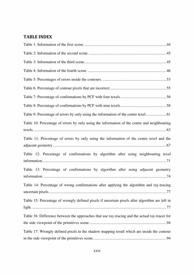
TABLE INDEX
Table 1: Information of the first scene. .................................................................................... 44
Table 2: Information of the second scene. ............................................................................... 45
Table 3: Information of the third scene. ................................................................................... 45
Table 4: Information of the fourth scene. ................................................................................ 46
Table 5: Percentages of errors inside the contours. ................................................................. 53
Table 6: Percentage of contour pixels that are incorrect. ......................................................... 55
Table 7: Percentage of confirmations by PCF with four texels. .............................................. 56
Table 8: Percentage of confirmations by PCF with nine texels. .............................................. 58
Table 9: Percentage of errors by only using the information of the centre texel. .................... 61
Table 10: Percentage of errors by only using the information of the centre and neighbouring
texels. ....................................................................................................................................... 63
Table 11: Percentage of errors by only using the information of the centre texel and the
adjacent geometry. ................................................................................................................... 67
Table 12: Percentage of confirmations by algorithm after using neighbouring texel
information. .............................................................................................................................. 71
Table 13: Percentage of confirmations by algorithm after using adjacent geometry
information. .............................................................................................................................. 74
Table 14: Percentage of wrong confirmations after applying the algorithm and ray-tracing
uncertain pixels. ....................................................................................................................... 77
Table 15: Percentage of wrongly defined pixels if uncertain pixels after algorithm are left in
light. ......................................................................................................................................... 77
Table 16: Difference between the approaches that use ray-tracing and the actual ray-tracer for
the side viewpoint of the primitives scene. .............................................................................. 94
Table 17: Wrongly defined pixels in the shadow mapping result which are inside the contour
in the side viewpoint of the primitives scene. .......................................................................... 94

xxx
Table 18: Pixels that the shadow map defines wrongly in the side viewpoint of the primitives
scene, separated in pixels defined in light and in shadow, compared to the total amount of
pixels lighted in the same way. ................................................................................................ 95
Table 19: Pixel confirmation when using texel coherence with four texels for the side
viewpoint of the primitives scene. ........................................................................................... 95
Table 20: Pixel shadowing for pixels that don’t achieve texel coherence with four texels for
the side viewpoint of the primitives scene. .............................................................................. 96
Table 21: Pixel confirmation when using texel coherence with nine texels for the side
viewpoint of the primitives scene. ........................................................................................... 96
Table 22: Pixel shadowing for pixels that don’t achieve texel coherence with nine texels for
the side viewpoint of the primitives scene. .............................................................................. 97
Table 23: Pixel correction between the single texel approach and the shadow mapping
approach for the side viewpoint of the primitives scene.......................................................... 98
Table 24: Pixel correction between the neighbour texels approach and the shadow mapping
approach for the side viewpoint of the primitives scene.......................................................... 98
Table 25: Average of triangle intersections when using the neighbour texels approach for the
side viewpoint of the primitives scene. .................................................................................... 99
Table 26: Pixel correction between the adjacent geometry approach and the shadow mapping
approach for the side viewpoint of the primitives scene........................................................ 100
Table 27: Average of triangle intersections when using the adjacent geometry approach for
the side viewpoint of the primitives scene. ............................................................................ 101
Table 28: Pixel correction by the neighbour texels (9 texels) and the adjacent geometry (2
levels) approaches separated by lighting change for the side viewpoint of the primitives
scene. ...................................................................................................................................... 102
Table 29: Algorithm results of the side viewpoint of the primitives scene. .......................... 103
Table 30: Difference between the approaches that use ray-tracing and the actual ray-tracer for
the with viewpoint of the primitives scene. ........................................................................... 111

xxxi
Table 31: Wrongly defined pixels in the shadow mapping result which are inside the contour
in the with viewpoint of the primitives scene. ....................................................................... 111
Table 32: Pixels that the shadow map defines wrongly in the with viewpoint of the primitives
scene, separated in pixels defined in light and in shadow, compared to the total amount of
pixels lighted in the same way. .............................................................................................. 112
Table 33: Pixel confirmation when using texel coherence with four texels for the with
viewpoint of the primitives scene. ......................................................................................... 112
Table 34: Pixel shadowing for pixels that don’t achieve texel coherence with four texels for
the with viewpoint of the primitives scene. ........................................................................... 113
Table 35: Pixel confirmation when using texel coherence with nine texels for the with
viewpoint of the primitives scene. ......................................................................................... 113
Table 36: Pixel shadowing for pixels that don’t achieve texel coherence with nine texels for
the with viewpoint of the primitives scene. ........................................................................... 114
Table 37: Pixel correction between the single texel approach and the shadow mapping
approach for the with viewpoint of the primitives scene. ...................................................... 115
Table 38: Pixel correction between the neighbour texels approach using four neighbours and
the shadow mapping approach for the with viewpoint of the primitives scene. .................... 115
Table 39: Pixel correction between the neighbour texels approach using nine neighbours and
the shadow mapping approach for the with viewpoint of the primitives scene. .................... 115
Table 40: Average of triangle intersections when using the neighbour texels approach for the
with viewpoint of the primitives scene. ................................................................................. 116
Table 41: Pixel correction between the adjacent geometry approach with one level of
adjacency and the shadow mapping approach for the with viewpoint of the primitives scene.
................................................................................................................................................ 116
Table 42: Pixel correction between the adjacent geometry approach with two levels of
adjacency and the shadow mapping approach for the with viewpoint of the primitives scene.
................................................................................................................................................ 116

xxxii
Table 43: Average of triangle intersections when using the adjacent geometry approach for
the with viewpoint of the primitives scene. ........................................................................... 117
Table 44: Pixel correction by the neighbour texels (9 texels) and the adjacent geometry (2
levels) approaches separated by lighting change for the with viewpoint of the primitives
scene. ...................................................................................................................................... 118
Table 45: Algorithm results of the with viewpoint of the primitives scene........................... 119
Table 46: Difference between the approaches that use ray-tracing and the actual ray-tracer for
the against viewpoint of the primitives scene. ....................................................................... 127
Table 47: Wrongly defined pixels in the shadow mapping result which are inside the contour
in the against viewpoint of the primitives scene. ................................................................... 127
Table 48: Pixels that the shadow map defines wrongly in the against viewpoint of the
primitives scene, separated in pixels defined in light and in shadow, compared to the total
amount of pixels lighted in the same way. ............................................................................. 128
Table 49: Pixel confirmation when using texel coherence with four texels for the against
viewpoint of the primitives scene. ......................................................................................... 128
Table 50: Pixel shadowing for pixels that don’t achieve texel coherence with four texels for
the against viewpoint of the primitives scene. ....................................................................... 129
Table 51: Pixel confirmation when using texel coherence with nine texels for the against
viewpoint of the primitives scene. ......................................................................................... 129
Table 52: Pixel shadowing for pixels that don’t achieve texel coherence with nine texels for
the against viewpoint of the primitives scene. ....................................................................... 130
Table 53: Pixel correction between the single texel approach and the shadow mapping
approach for the against viewpoint of the primitives scene. .................................................. 131
Table 54: Pixel correction between the neighbour texels approach using four neighbours and
the shadow mapping approach for the against viewpoint of the primitives scene. ................ 131
Table 55: Pixel correction between the neighbour texels approach using nine neighbours and
the shadow mapping approach for the against viewpoint of the primitives scene. ................ 131

xxxiii
Table 56: Average of triangle intersections when using the neighbour texels approach for the
against viewpoint of the primitives scene. ............................................................................. 132
Table 57: Pixel correction between the adjacent geometry approach with one level of
adjacency and the shadow mapping approach for the against viewpoint of the primitives
scene. ...................................................................................................................................... 132
Table 58: Pixel correction between the adjacent geometry approach with two levels of
adjacency and the shadow mapping approach for the against viewpoint of the primitives
scene. ...................................................................................................................................... 132
Table 59: Average of triangle intersections when using the adjacent geometry approach for
the against viewpoint of the primitives scene. ....................................................................... 133
Table 60: Pixel correction by the neighbour texels (9 texels) and the adjacent geometry (2
levels) approaches separated by lighting change for the against viewpoint of the primitives
scene. ...................................................................................................................................... 134
Table 61: Algorithm results of the against viewpoint of the primitives scene. ..................... 135
Table 62: Difference between the approaches that use ray-tracing and the actual ray-tracer for
the side viewpoint of the bench scene.................................................................................... 143
Table 63: Wrongly defined pixels in the shadow mapping result which are inside the contour
in the side viewpoint of the bench scene. .............................................................................. 143
Table 64: Pixels that the shadow map defines wrongly in the side viewpoint of the bench
scene, separated in pixels defined in light and in shadow, compared to the total amount of
pixels lighted in the same way. .............................................................................................. 144
Table 65: Pixel confirmation when using texel coherence with four texels for the side
viewpoint of the bench scene. ................................................................................................ 144
Table 66: Pixel shadowing for pixels that don’t achieve texel coherence with four texels for
the side viewpoint of the bench scene.................................................................................... 145
Table 67: Pixel confirmation when using texel coherence with nine texels for the side
viewpoint of the bench scene. ................................................................................................ 145

xxxiv
Table 68: Pixel shadowing for pixels that don’t achieve texel coherence with nine texels for
the side viewpoint of the bench scene.................................................................................... 146
Table 69: Pixel correction between the single texel approach and the shadow mapping
approach for the side viewpoint of the bench scene. ............................................................. 147
Table 70: Pixel correction between the neighbour texels approach using four neighbours and
the shadow mapping approach for the side viewpoint of the bench scene. ........................... 147
Table 71: Pixel correction between the neighbour texels approach using nine neighbours and
the shadow mapping approach for the side viewpoint of the bench scene. ........................... 147
Table 72: Average of triangle intersections when using the neighbour texels approach for the
side viewpoint of the bench scene. ........................................................................................ 148
Table 73: Pixel correction between the adjacent geometry approach with one level of
adjacency and the shadow mapping approach for the side viewpoint of the bench scene. ... 148
Table 74: Pixel correction between the adjacent geometry approach with two levels of
adjacency and the shadow mapping approach for the side viewpoint of the bench scene. ... 148
Table 75: Average of triangle intersections when using the adjacent geometry approach for
the side viewpoint of the bench scene.................................................................................... 149
Table 76: Pixel correction by the neighbour texels (9 texels) and the adjacent geometry (2
levels) approaches separated by lighting change for the side viewpoint of the bench scene. 150
Table 77: Algorithm results of the side viewpoint of the bench scene. ................................. 151
Table 78: Difference between the approaches that use ray-tracing and the actual ray-tracer for
the with viewpoint of the bench scene. .................................................................................. 159
Table 79: Wrongly defined pixels in the shadow mapping result which are inside the contour
in the with viewpoint of the bench scene. .............................................................................. 159
Table 80: Pixels that the shadow map defines wrongly in the with viewpoint of the bench
scene, separated in pixels defined in light and in shadow, compared to the total amount of
pixels lighted in the same way. .............................................................................................. 160

xxxv
Table 81: Pixel confirmation when using texel coherence with four texels for the with
viewpoint of the bench scene. ................................................................................................ 160
Table 82: Pixel shadowing for pixels that don’t achieve texel coherence with four texels for
the with viewpoint of the bench scene. .................................................................................. 161
Table 83: Pixel confirmation when using texel coherence with nine texels for the with
viewpoint of the bench scene. ................................................................................................ 161
Table 84: Pixel shadowing for pixels that don’t achieve texel coherence with nine texels for
the with viewpoint of the bench scene. .................................................................................. 162
Table 85: Pixel correction between the single texel approach and the shadow mapping
approach for the with viewpoint of the bench scene. ............................................................. 163
Table 86: Pixel correction between the neighbour texels approach using four neighbours and
the shadow mapping approach for the with viewpoint of the bench scene. .......................... 163
Table 87: Pixel correction between the neighbour texels approach using nine neighboursand
the shadow mapping approach for the with viewpoint of the bench scene. .......................... 163
Table 88: Average of triangle intersections when using the neighbour texels approach for the
with viewpoint of the bench scene. ........................................................................................ 164
Table 89: Pixel correction between the adjacent geometry approach with one level of
adjacency and the shadow mapping approach for the with viewpoint of the bench scene. ... 164
Table 90: Pixel correction between the adjacent geometry approach with two levels of
adjacency and the shadow mapping approach for the with viewpoint of the bench scene. ... 164
Table 91: Average of triangle intersections when using the adjacent geometry approach for
the with viewpoint of the bench scene. .................................................................................. 165
Table 92: Pixel correction by the neighbour texels (9 texels) and the adjacent geometry (2
levels) approaches separated by lighting change for the with viewpoint of the bench scene.
................................................................................................................................................ 166
Table 93: Algorithm results of the with viewpoint of the bench scene. ................................ 167

xxxvi
Table 94: Difference between the approaches that use ray-tracing and the actual ray-tracer for
the against viewpoint of the bench scene. .............................................................................. 175
Table 95: Wrongly defined pixels in the shadow mapping result which are inside the contour
in the against viewpoint of the bench scene. .......................................................................... 175
Table 96: Pixels that the shadow map defines wrongly in the against viewpoint of the bench
scene, separated in pixels defined in light and in shadow, compared to the total amount of
pixels lighted in the same way. .............................................................................................. 176
Table 97: Pixel confirmation when using texel coherence with four texels for the against
viewpoint of the bench scene. ................................................................................................ 176
Table 98: Pixel shadowing for pixels that don’t achieve texel coherence with four texels for
the against viewpoint of the bench scene. .............................................................................. 177
Table 99: Pixel confirmation when using texel coherence with nine texels for the against
viewpoint of the bench scene. ................................................................................................ 177
Table 100: Pixel shadowing for pixels that don’t achieve texel coherence with nine texels for
the against viewpoint of the bench scene. .............................................................................. 178
Table 101: Pixel correction between the single texel approach and the shadow mapping
approach for the against viewpoint of the bench scene. ........................................................ 179
Table 102: Pixel correction between the neighbour texels approach and the shadow mapping
approach for the against viewpoint of the bench scene. ........................................................ 180
Table 103: Average of triangle intersections when using the neighbour texels approach for
the against viewpoint of the bench scene. .............................................................................. 181
Table 104: Pixel correction between the adjacent geometry approach and the shadow
mapping approach for the against viewpoint of the bench scene. ......................................... 182
Table 105: Average of triangle intersections when using the adjacent geometry approach for
the against viewpoint of the bench scene. .............................................................................. 183
Table 106: Pixel correction by the neighbour texels (9 texels) and the adjacent geometry (2
levels) approaches separated by lighting change for the against viewpoint of the bench scene.
................................................................................................................................................ 184

xxxvii
Table 107: Algorithm results of the against viewpoint of the bench scene. .......................... 185
Table 108: Difference between the approaches that use ray-tracing and the actual ray-tracer
for the with viewpoint of the trees scene. .............................................................................. 193
Table 109: Wrongly defined pixels in the shadow mapping result which are inside the contour
in the with viewpoint of the trees scene. ................................................................................ 193
Table 110: Pixels that the shadow map defines wrongly in the with viewpoint of the trees
scene, separated in pixels defined in light and in shadow, compared to the total amount of
pixels lighted in the same way. .............................................................................................. 194
Table 111: Pixel confirmation when using texel coherence with four texels for the with
viewpoint of the trees scene. .................................................................................................. 194
Table 112: Pixel shadowing for pixels that don’t achieve texel coherence with four texels for
the with viewpoint of the trees scene. .................................................................................... 195
Table 113: Pixel confirmation when using texel coherence with nine texels for the with
viewpoint of the trees scene. .................................................................................................. 195
Table 114: Pixel shadowing for pixels that don’t achieve texel coherence with nine texels for
the with viewpoint of the trees scene. .................................................................................... 196
Table 115: Pixel correction between the single texel approach and the shadow mapping
approach for the with viewpoint of the trees scene. ............................................................... 197
Table 116: Pixel correction between the neighbour texels approach and the shadow mapping
approach for the with viewpoint of the trees scene. ............................................................... 197
Table 117: Average of triangle intersections when using the neighbour texels approach for
the with viewpoint of the trees scene. .................................................................................... 198
Table 118: Pixel correction between the adjacent geometry approach and the shadow
mapping approach for the with viewpoint of the trees scene................................................. 199
Table 119: Average of triangle intersections when using the adjacent geometry approach for
the with viewpoint of the trees scene. .................................................................................... 200

xxxviii
Table 120: Pixel correction by the neighbour texels (9 texels) and the adjacent geometry (2
levels) approaches separated by lighting change for the with viewpoint of the trees scene. . 201
Table 121: Algorithm results of the with viewpoint of the trees scene. ................................ 202
Table 122: Difference between the approaches that use ray-tracing and the actual ray-tracer
for the side viewpoint of the trees scene. ............................................................................... 210
Table 123: Wrongly defined pixels in the shadow mapping result which are inside the contour
in the side viewpoint of the trees scene. ................................................................................ 210
Table 124: Pixels that the shadow map defines wrongly in the side viewpoint of the trees
scene, separated in pixels defined in light and in shadow, compared to the total amount of
pixels lighted in the same way. .............................................................................................. 211
Table 125: Pixel confirmation when using texel coherence with four texels for the side
viewpoint of the trees scene. .................................................................................................. 211
Table 126: Pixel shadowing for pixels that don’t achieve texel coherence with four texels for
the side viewpoint of the trees scene...................................................................................... 212
Table 127: Pixel confirmation when using texel coherence with nine texels for the side
viewpoint of the trees scene. .................................................................................................. 212
Table 128: Pixel shadowing for pixels that don’t achieve texel coherence with nine texels for
the side viewpoint of the trees scene...................................................................................... 213
Table 129: Pixel correction between the single texel approach and the shadow mapping
approach for the side viewpoint of the trees scene. ............................................................... 214
Table 130: Pixel correction between the neighbour texels approach using four neighbours and
the shadow mapping approach for the side viewpoint of the trees scene. ............................. 214
Table 131: Pixel correction between the neighbour texels approach using nine neighbours and
the shadow mapping approach for the side viewpoint of the trees scene. ............................. 214
Table 132: Average of triangle intersections when using the neighbour texels approach for
the side viewpoint of the trees scene...................................................................................... 215

xxxix
Table 133: Pixel correction between the adjacent geometry approach with one level of
adjacency and the shadow mapping approach for the side viewpoint of the trees scene. ..... 215
Table 134: Pixel correction between the adjacent geometry approach with two level of
adjacency and the shadow mapping approach for the side viewpoint of the trees scene. ..... 215
Table 135: Average of triangle intersections when using the adjacent geometry approach for
the side viewpoint of the trees scene...................................................................................... 216
Table 136: Pixel correction by the neighbour texels (9 texels) and the adjacent geometry (2
levels) approaches separated by lighting change for the side viewpoint of the trees scene. . 217
Table 137: Algorithm results of the side viewpoint of the trees scene. ................................. 218
Table 138: Difference between the approaches that use ray-tracing and the actual ray-tracer
for the against viewpoint of the trees scene. .......................................................................... 226
Table 139: Wrongly defined pixels in the shadow mapping result which are inside the contour
in the against viewpoint of the trees scene. ............................................................................ 226
Table 140: Pixels that the shadow map defines wrongly in the against viewpoint of the trees
scene, separated in pixels defined in light and in shadow, compared to the total amount of
pixels lighted in the same way. .............................................................................................. 227
Table 141: Pixel confirmation when using texel coherence with four texels for the against
viewpoint of the trees scene. .................................................................................................. 227
Table 142: Pixel shadowing for pixels that don’t achieve texel coherence with four texels for
the against viewpoint of the trees scene. ................................................................................ 228
Table 143: Pixel confirmation when using texel coherence with nine texels for the against
viewpoint of the trees scene. .................................................................................................. 228
Table 144: Pixel shadowing for pixels that don’t achieve texel coherence with nine texels for
the against viewpoint of the trees scene. ................................................................................ 229
Table 145: Pixel correction between the single texel approach and the shadow mapping
approach for the against viewpoint of the trees scene. .......................................................... 230

xl
Table 146: Pixel correction between the neighbour texels approach using four neighbours and
the shadow mapping approach for the against viewpoint of the trees scene. ........................ 230
Table 147: Pixel correction between the neighbour texels approach using nine neighbours and
the shadow mapping approach for the against viewpoint of the trees scene. ........................ 230
Table 148: Average of triangle intersections when using the neighbour texels approach for
the against viewpoint of the trees scene. ................................................................................ 231
Table 149: Pixel correction between the adjacent geometry approach with one level of
adjacency and the shadow mapping approach for the against viewpoint of the trees scene. 231
Table 150: Pixel correction between the adjacent geometry approach with two level of
adjacency and the shadow mapping approach for the against viewpoint of the trees scene. 231
Table 151: Average of triangle intersections when using the adjacent geometry approach for
the against viewpoint of the trees scene. ................................................................................ 232
Table 152: Pixel correction by the neighbour texels (9 texels) and the adjacent geometry (2
levels) approaches separated by lighting change for the against viewpoint of the trees scene.
................................................................................................................................................ 233
Table 153: Algorithm results of the against viewpoint of the trees scene. ............................ 234
Table 154: Difference between the approaches that use ray-tracing and the actual ray-tracer
for the side viewpoint of the flowers scene. .......................................................................... 242
Table 155: Wrongly defined pixels in the shadow mapping result which are inside the contour
in the side viewpoint of the flowers scene. ............................................................................ 242
Table 156: Pixels that the shadow map defines wrongly in the side viewpoint of the flowers
scene, separated in pixels defined in light and in shadow, compared to the total amount of
pixels lighted in the same way. .............................................................................................. 243
Table 157: Pixel confirmation when using texel coherence with four texels for the side
viewpoint of the flowers scene. ............................................................................................. 243
Table 158: Pixel shadowing for pixels that don’t achieve texel coherence with four texels for
the side viewpoint of the flowers scene. ................................................................................ 244
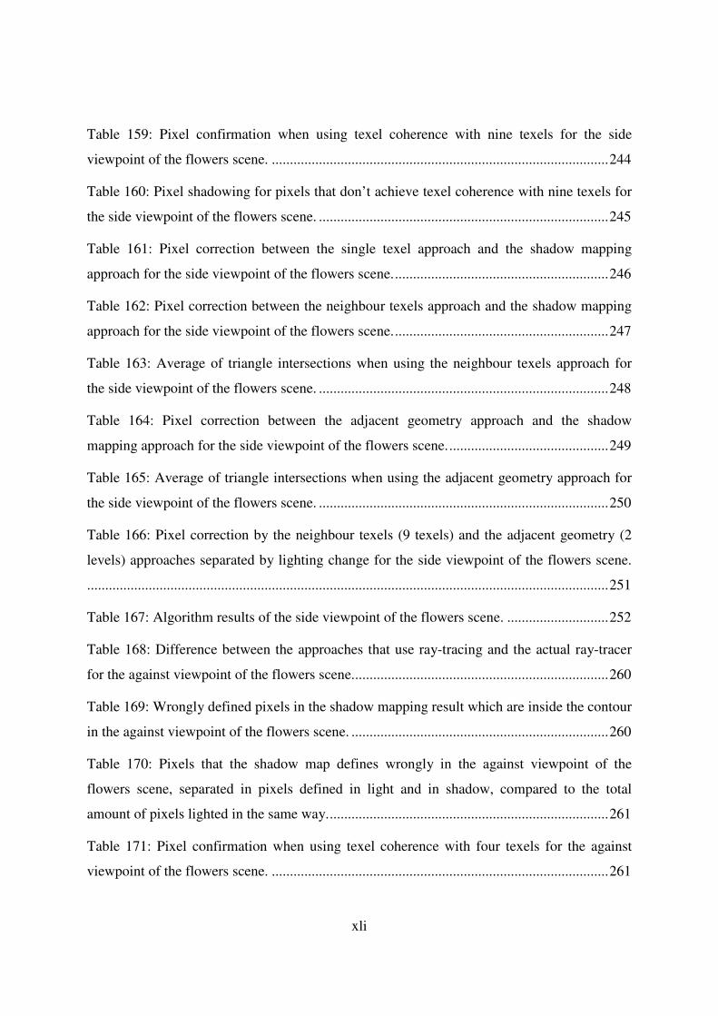
xli
Table 159: Pixel confirmation when using texel coherence with nine texels for the side
viewpoint of the flowers scene. ............................................................................................. 244
Table 160: Pixel shadowing for pixels that don’t achieve texel coherence with nine texels for
the side viewpoint of the flowers scene. ................................................................................ 245
Table 161: Pixel correction between the single texel approach and the shadow mapping
approach for the side viewpoint of the flowers scene. ........................................................... 246
Table 162: Pixel correction between the neighbour texels approach and the shadow mapping
approach for the side viewpoint of the flowers scene. ........................................................... 247
Table 163: Average of triangle intersections when using the neighbour texels approach for
the side viewpoint of the flowers scene. ................................................................................ 248
Table 164: Pixel correction between the adjacent geometry approach and the shadow
mapping approach for the side viewpoint of the flowers scene. ............................................ 249
Table 165: Average of triangle intersections when using the adjacent geometry approach for
the side viewpoint of the flowers scene. ................................................................................ 250
Table 166: Pixel correction by the neighbour texels (9 texels) and the adjacent geometry (2
levels) approaches separated by lighting change for the side viewpoint of the flowers scene.
................................................................................................................................................ 251
Table 167: Algorithm results of the side viewpoint of the flowers scene. ............................ 252
Table 168: Difference between the approaches that use ray-tracing and the actual ray-tracer
for the against viewpoint of the flowers scene....................................................................... 260
Table 169: Wrongly defined pixels in the shadow mapping result which are inside the contour
in the against viewpoint of the flowers scene. ....................................................................... 260
Table 170: Pixels that the shadow map defines wrongly in the against viewpoint of the
flowers scene, separated in pixels defined in light and in shadow, compared to the total
amount of pixels lighted in the same way. ............................................................................. 261
Table 171: Pixel confirmation when using texel coherence with four texels for the against
viewpoint of the flowers scene. ............................................................................................. 261

xlii
Table 172: Pixel shadowing for pixels that don’t achieve texel coherence with four texels for
the against viewpoint of the flowers scene. ........................................................................... 262
Table 173: Pixel confirmation when using texel coherence with nine texels for the against
viewpoint of the flowers scene. ............................................................................................. 262
Table 174: Pixel shadowing for pixels that don’t achieve texel coherence with nine texels for
the against viewpoint of the flowers scene. ........................................................................... 263
Table 175: Pixel correction between the single texel approach and the shadow mapping
approach for the against viewpoint of the flowers scene. ...................................................... 264
Table 176: Pixel correction between the neighbour texels approach using four neighbours and
the shadow mapping approach for the against viewpoint of the flowers scene. .................... 264
Table 177: Pixel correction between the neighbour texels approach using nine neighbours and
the shadow mapping approach for the against viewpoint of the flowers scene. .................... 264
Table 178: Average of triangle intersections when using the neighbour texels approach for
the against viewpoint of the flowers scene. ........................................................................... 265
Table 179: Pixel correction between the adjacent geometry approach with one level of
adjacency and the shadow mapping approach for the against viewpoint of the flowers scene.
................................................................................................................................................ 265
Table 180: Pixel correction between the adjacent geometry approach with two level of
adjacency and the shadow mapping approach for the against viewpoint of the flowers scene.
................................................................................................................................................ 265
Table 181: Average of triangle intersections when using the adjacent geometry approach for
the against viewpoint of the flowers scene. ........................................................................... 266
Table 182: Pixel correction by the neighbour texels (9 texels) and the adjacent geometry (2
levels) approaches separated by lighting change for the against viewpoint of the flowers
scene. ...................................................................................................................................... 267
Table 183: Algorithm results of the against viewpoint of the flowers scene......................... 268
Table 184: Difference between the approaches that use ray-tracing and the actual ray-tracer
for the with viewpoint of the flowers scene. .......................................................................... 276

xliii
Table 185: Wrongly defined pixels in the shadow mapping result which are inside the contour
in the with viewpoint of the flowers scene. ........................................................................... 276
Table 186: Pixels that the shadow map defines wrongly in the with viewpoint of the flowers
scene, separated in pixels defined in light and in shadow, compared to the total amount of
pixels lighted in the same way. .............................................................................................. 277
Table 187: Pixel confirmation when using texel coherence with four texels for the with
viewpoint of the flowers scene. ............................................................................................. 277
Table 188: Pixel shadowing for pixels that don’t achieve texel coherence with four texels for
the with viewpoint of the flowers scene. ............................................................................... 278
Table 189: Pixel confirmation when using texel coherence with nine texels for the with
viewpoint of the flowers scene. ............................................................................................. 278
Table 190: Pixel shadowing for pixels that don’t achieve texel coherence with nine texels for
the with viewpoint of the flowers scene. ............................................................................... 279
Table 191: Pixel correction between the single texel approach and the shadow mapping
approach for the with viewpoint of the flowers scene. .......................................................... 280
Table 192: Pixel correction between the neighbour texels approach using four neighbours and
the shadow mapping approach for the with viewpoint of the flowers scene. ........................ 280
Table 193: Pixel correction between the neighbour texels approach using nine neighbours and
the shadow mapping approach for the with viewpoint of the flowers scene. ........................ 280
Table 194: Average of triangle intersections when using the neighbour texels approach for
the with viewpoint of the flowers scene. ............................................................................... 281
Table 195: Pixel correction between the adjacent geometry approach with one level of
adjacency and the shadow mapping approach for the with viewpoint of the flowers scene. 281
Table 196: Pixel correction between the adjacent geometry approach with two level of
adjacency and the shadow mapping approach for the with viewpoint of the flowers scene. 281
Table 197: Average of triangle intersections when using the adjacent geometry approach for
the with viewpoint of the flowers scene. ............................................................................... 282

xliv
Table 198: Pixel correction by the neighbour texels (9 texels) and the adjacent geometry (2
levels) approaches separated by lighting change for the with viewpoint of the flowers scene.
................................................................................................................................................ 283
Table 199: Algorithm results of the with viewpoint of the flowers scene. ............................ 284
1
1. INTRODUCTION
Since the appearance of computer rendered graphics, there have been two main approaches in
order to render scenes: the first one is to obtain satisfactory images in a fraction of a second
and the other is to obtain the best quality images, with no regard to the time spent in creating
them. Both of these approaches have their uses, with the first one being important to real time
rendering used in virtual interactive walkthroughs, and the second being used to create photo-
realistic scenes, be it for simple images or for use in a frame of an animated movie.
One of the most important things in rendering a scene is lighting and consequently, shadows.
While it is possible to render shadowed scenes in real time, there is clearly a loss in quality
when comparing to more computationally intensive algorithms. Shadow algorithms are
available for hard and soft shadows, where being able to establish the former is required for
the latter. Hence hard shadows are a very relevant topic.
Real-time rendering shadow algorithms are dominated by two classes: shadow maps and
shadow volumes. Shadow volumes are able to compute pixel perfect shadows yet are harder
to implement and can suffer from severe overdrawing. Shadow maps, on the other hand, are
very simple to implement, and are performance friendly.
Recent research has focused on improving the quality of the shadow map basic algorithm
result, for instance combining it with other algorithms. Shadow maps have evolved a lot,
fixing and improving the basic algorithm, hence providing better and better results.
Another solution that is now possible in real time (at least for direct hard shadows) is ray-
tracing. However shadow mapping is much faster than ray-tracing, and while ray-tracing is
now a possibility for real-time rendering, one has to consider that the quality standards have
gone sky high and hard shadows are not jaw dropping anymore. Shadows are only one of
many effects that are used nowadays to improve render quality hence shadows must be
computed as fast as possible.
2
1.1. MOTIVATION
As mentioned before, ray-tracing and shadow maps are two possibilities for computing hard
shadows in real-time. Ray-tracing assures that the result is correct for each pixel, where
shadow maps guarantee performance. The ideal would be to have the performance of shadow
maps with the quality of ray-tracing, or at least some compromise that would improve quality
without totally sacrificing performance.
Research has been conducted to achieve the best of both worlds: great quality images that
take a small amount of time to render. However, so far no research has been performed to
evaluate how good the information stored in a shadow map really is.
1.2. GOALS
Studying the value of the information stored in a shadow map is the main goal of this work.
For instance, quantifying the location of the errors in a shadow map, or how many texels in a
shadow map are actually correct, i.e. report the closest triangle to the light in a given
direction. And how far can an algorithm improve the basic shadow map just using the
information stored in it? For instance, can the shadow map information be used to perform
selective ray-tracing for certain pixels, and if so how many pixels are fixed and how many
pixels are broken? Although some algorithms use this information to perform selective ray-
tracing the published work only focuses on particular cases.
When using shadow mapping to evaluate the shadow areas of a scene, the most problematic
areas are the contour regions where the real shadow occurs due to the lack of precision, and
aliasing of the shadow mapping technique. Hence, when studying the quality of a solution
based on shadow mapping it makes sense to concentrate efforts in the contours of the shadow
map. But how thick must a contour be to contain a significant number of wrong pixels? And
for those pixels in the contours which approaches can be used, based only on the shadow map
information, to validate or fix their shadow status?
Ray-tracing can be a helpful tool, helping in fixing a number of pixels, but is the shadow map
information sufficient so that the number of rays is cut down to a very low number? And can
3
pixels be fixed with just a very small number of ray-triangle intersections, where the triangles
are selected based on the information stored in the shadow map?
By limiting the number of ray-triangle intersections new errors will be introduced. Hence
quantifying the ratio of fixed/broken pixels, when performing this second pass, is essential to
evaluate each approach or approach combinations.
The goal of this work is to provide an answer to these questions, with a quantitative analysis.
1.3. METHODOLOGY
The Curitiba 3D engine is capable of using shadow maps and provides a lot of debug
information. It is an extensible engine and adding the required features to quantify
information, and test new algorithms is really easy. However no ray-tracing is available in
Curitiba, hence the first step was to implement a very basic ray-tracer. This new
implementation will contain the required functionalities to provide the answers required for
this work. However no performance issues were taken into account due to the timeframe
required for the completion of the work.
Once the implementation was completed focus could be directed on studying the shadow map
generation process. This provided some clues to the type of problems one can expect when
applying shadow maps. The next step was to determine where the majority of errors were
located.
Then a study on the pixel shadow status versus its correctness was conducted and hypotheses
on how to fix the pixels shadow status were constructed.
Each hypothesis was tested and its results quantified. This in turn gave rise to new hypothesis
and the process was iterated and finally hypotheses were combined to evaluate if better
results were obtained. Selective ray-tracing with a very limited number of ray-triangle
intersections, where the triangles were selected based on the shadow map information, was
used to attempt to fix pixels.
During all this process the ray-tracer for the whole image was used as ground truth, and each
hypothesis, or combination, was tested both against the ground truth and the shadow map
basic solution.

4
1.4. THESIS STRUCTURE
In chapter 2 the state of the art for the shadow mapping and ray-tracing algorithms will be
shown. In chapter 3 the main research of this work, as described in the motivation and goals
section is presented. Chapter 4 will report on the tests made and present the results obtained.
Finally, chapter 5 will present the conclusion of this work and point to some possible future
work.
5
2. STATE OF THE ART
This chapter will present the state of the art of the shadow mapping and ray tracing
algorithms. To be precise, this chapter will show how each one of these algorithms work, the
problems that these algorithms have and various approaches proposed to solve these
shortcomings. Finally, some approaches that combine both algorithms will be presented, also
summarizing how they work and some of their problems.
2.1. SHADOW MAPPING
2.1.1. Shadow Mapping Basics
Shadow Mapping (Williams, 1978) is an algorithm that defines shadows in the scene by
determining which areas are behind the closest objects to the light source. This is done in a
two-step approach:
1. First, the algorithm renders the scene from the point of view of the light source, saving the
shortest distances between the light source and the scene’s triangles in the rendered grid. The
information of each grid point will be called a shadow texel and the entire grid of shadow
texels will be called the shadow map.
2. After obtaining the shadow map, the scene will be rendered from the point of view of the
camera. Each 3D point that the camera sees will be tested, in order to verify if it is in the
shadow of the light source. In order to do this, each point will be transformed from the
coordinates of the camera view to the coordinates of the view of the light source view. With
the new coordinates, the algorithm will be able to check which texel in the shadow map
intersects the ray that goes from the source of light to the point that is being tested. Finally,
the distance to the light source of the point being tested is compared to the distance stored in
the texel of the shadow map. If the distance of the point being tested is greater than the stored
distance, then it will be shadowed, otherwise, it will not.
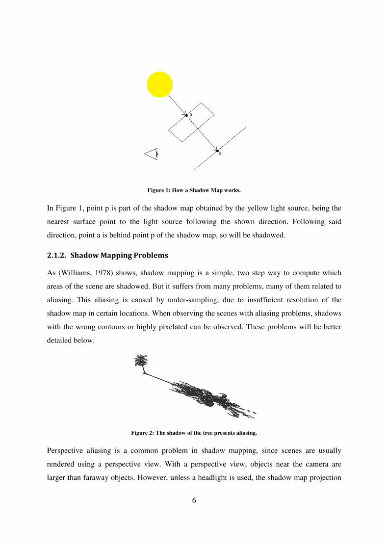
6
Figure 1: How a Shadow Map works.
In Figure 1, point p is part of the shadow map obtained by the yellow light source, being the
nearest surface point to the light source following the shown direction. Following said
direction, point a is behind point p of the shadow map, so will be shadowed.
2.1.2. Shadow Mapping Problems
As (Williams, 1978) shows, shadow mapping is a simple, two step way to compute which
areas of the scene are shadowed. But it suffers from many problems, many of them related to
aliasing. This aliasing is caused by under-sampling, due to insufficient resolution of the
shadow map in certain locations. When observing the scenes with aliasing problems, shadows
with the wrong contours or highly pixelated can be observed. These problems will be better
detailed below.
Figure 2: The shadow of the tree presents aliasing.
Perspective aliasing is a common problem in shadow mapping, since scenes are usually
rendered using a perspective view. With a perspective view, objects near the camera are
larger than faraway objects. However, unless a headlight is used, the shadow map projection
7
is not the same as the camera´s. This creates a resolution mismatch. The problem appears
when there are a lot of points near the camera, but these same points are distant from the light
source. Due to the perspective view, a large amount of these points will be behind a single
shadow texel, which will provoke aliasing in the shadow. On the other hand, there may be
places far away in the camera view where the texel resolution is excessive, resulting in
wasted shadow texels. Both these cases are called, respectively, under-sampling and over-
sampling.
With a directional light, this mismatch will have its maximum value if the direction of this
light is perpendicular to the camera view and will have its minimum value when the light
direction is the same as the camera view. For point lights, the mismatch will be greater when
the direction of the light and the camera views face each other, a.k.a. the duelling frusta, and
minimum when both have the same direction.
Projection aliasing occurs when a surface is parallel (or almost parallel) to the direction of the
light. In this case, a single shadow texel will be used to test the occlusion of the light source
for a large amount of points, which will cause incorrect shadows. Another problem that
comes with projection aliasing is shadow flickering when moving around the scene. This
occurs because the perspective aliasing effect is dependent on the position and direction of
the camera.
The resolution of the shadow map may also be a problem if it is used for large scenes. The
shadow map is usually saved as a texture, but today's hardware limits the size of textures,
which limits the size of the shadow map. For example, for a scene with one square kilometre
and a perpendicular light direction, a 1024x1024 shadow map has shadow texels that take
around one square meter each. While this may give satisfactory results for a bird’s eye view
over the entire scene, a close-up of this scene will show a large amount of aliasing.
Due to the limited precision of data in computers, calculated distances are in general not
exact, but actually an approximation to the real value. Furthermore, the grid that stores the
shadow map and the final viewed image are also discrete. These discrete properties and these
approximations may cause distances to be calculated in an erroneous way. In the case where
the calculated distance of a point to the light source during the second step of the algorithm
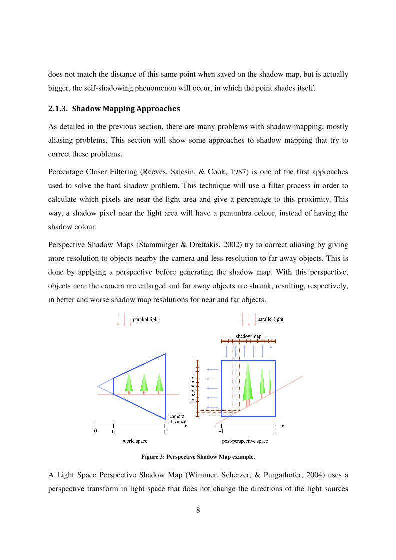
8
does not match the distance of this same point when saved on the shadow map, but is actually
bigger, the self-shadowing phenomenon will occur, in which the point shades itself.
2.1.3. Shadow Mapping Approaches
As detailed in the previous section, there are many problems with shadow mapping, mostly
aliasing problems. This section will show some approaches to shadow mapping that try to
correct these problems.
Percentage Closer Filtering (Reeves, Salesin, & Cook, 1987) is one of the first approaches
used to solve the hard shadow problem. This technique will use a filter process in order to
calculate which pixels are near the light area and give a percentage to this proximity. This
way, a shadow pixel near the light area will have a penumbra colour, instead of having the
shadow colour.
Perspective Shadow Maps (Stamminger & Drettakis, 2002) try to correct aliasing by giving
more resolution to objects nearby the camera and less resolution to far away objects. This is
done by applying a perspective before generating the shadow map. With this perspective,
objects near the camera are enlarged and far away objects are shrunk, resulting, respectively,
in better and worse shadow map resolutions for near and far objects.
Figure 3: Perspective Shadow Map example.
A Light Space Perspective Shadow Map (Wimmer, Scherzer, & Purgathofer, 2004) uses a
perspective transform in light space that does not change the directions of the light sources
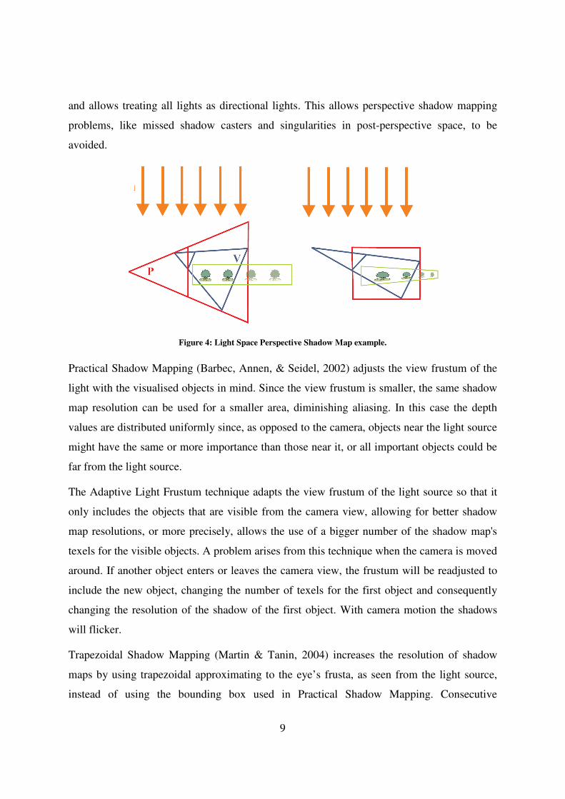
9
and allows treating all lights as directional lights. This allows perspective shadow mapping
problems, like missed shadow casters and singularities in post-perspective space, to be
avoided.
Figure 4: Light Space Perspective Shadow Map example.
Practical Shadow Mapping (Barbec, Annen, & Seidel, 2002) adjusts the view frustum of the
light with the visualised objects in mind. Since the view frustum is smaller, the same shadow
map resolution can be used for a smaller area, diminishing aliasing. In this case the depth
values are distributed uniformly since, as opposed to the camera, objects near the light source
might have the same or more importance than those near it, or all important objects could be
far from the light source.
The Adaptive Light Frustum technique adapts the view frustum of the light source so that it
only includes the objects that are visible from the camera view, allowing for better shadow
map resolutions, or more precisely, allows the use of a bigger number of the shadow map's
texels for the visible objects. A problem arises from this technique when the camera is moved
around. If another object enters or leaves the camera view, the frustum will be readjusted to
include the new object, changing the number of texels for the first object and consequently
changing the resolution of the shadow of the first object. With camera motion the shadows
will flicker.
Trapezoidal Shadow Mapping (Martin & Tanin, 2004) increases the resolution of shadow
maps by using trapezoidal approximating to the eye’s frusta, as seen from the light source,
instead of using the bounding box used in Practical Shadow Mapping. Consecutive
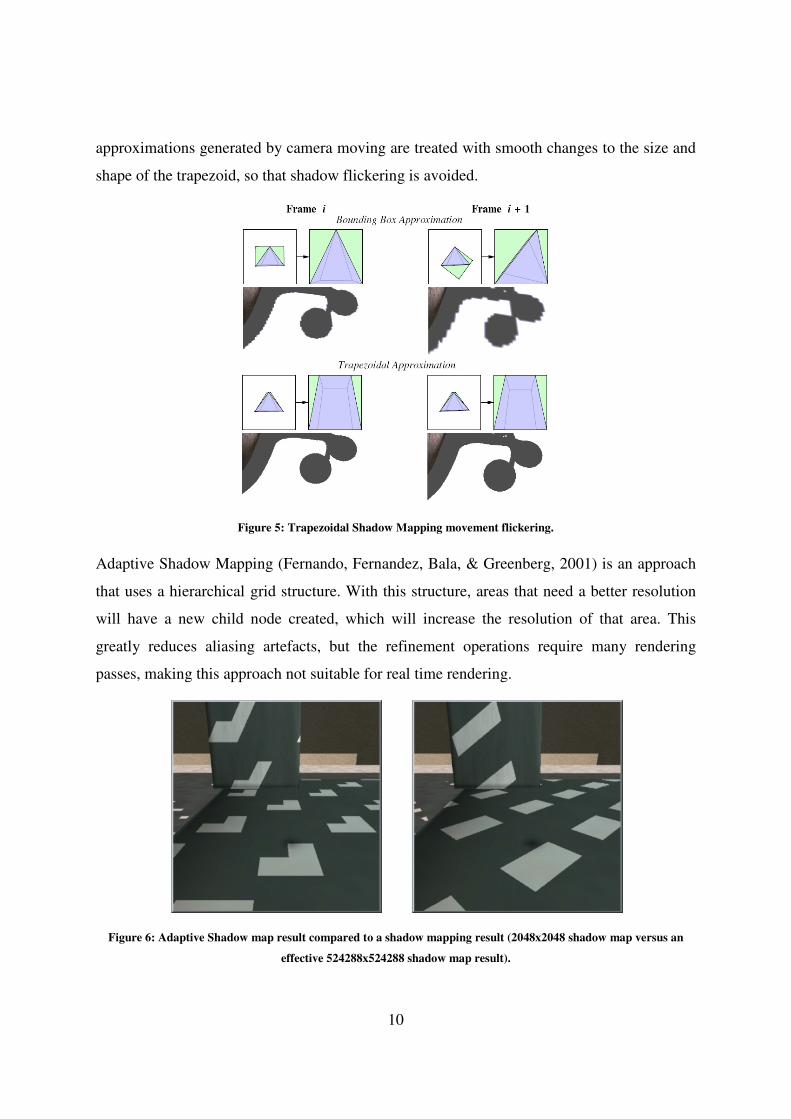
10
approximations generated by camera moving are treated with smooth changes to the size and
shape of the trapezoid, so that shadow flickering is avoided.
Figure 5: Trapezoidal Shadow Mapping movement flickering.
Adaptive Shadow Mapping (Fernando, Fernandez, Bala, & Greenberg, 2001) is an approach
that uses a hierarchical grid structure. With this structure, areas that need a better resolution
will have a new child node created, which will increase the resolution of that area. This
greatly reduces aliasing artefacts, but the refinement operations require many rendering
passes, making this approach not suitable for real time rendering.
Figure 6: Adaptive Shadow map result compared to a shadow mapping result (2048x2048 shadow map versus an
effective 524288x524288 shadow map result).
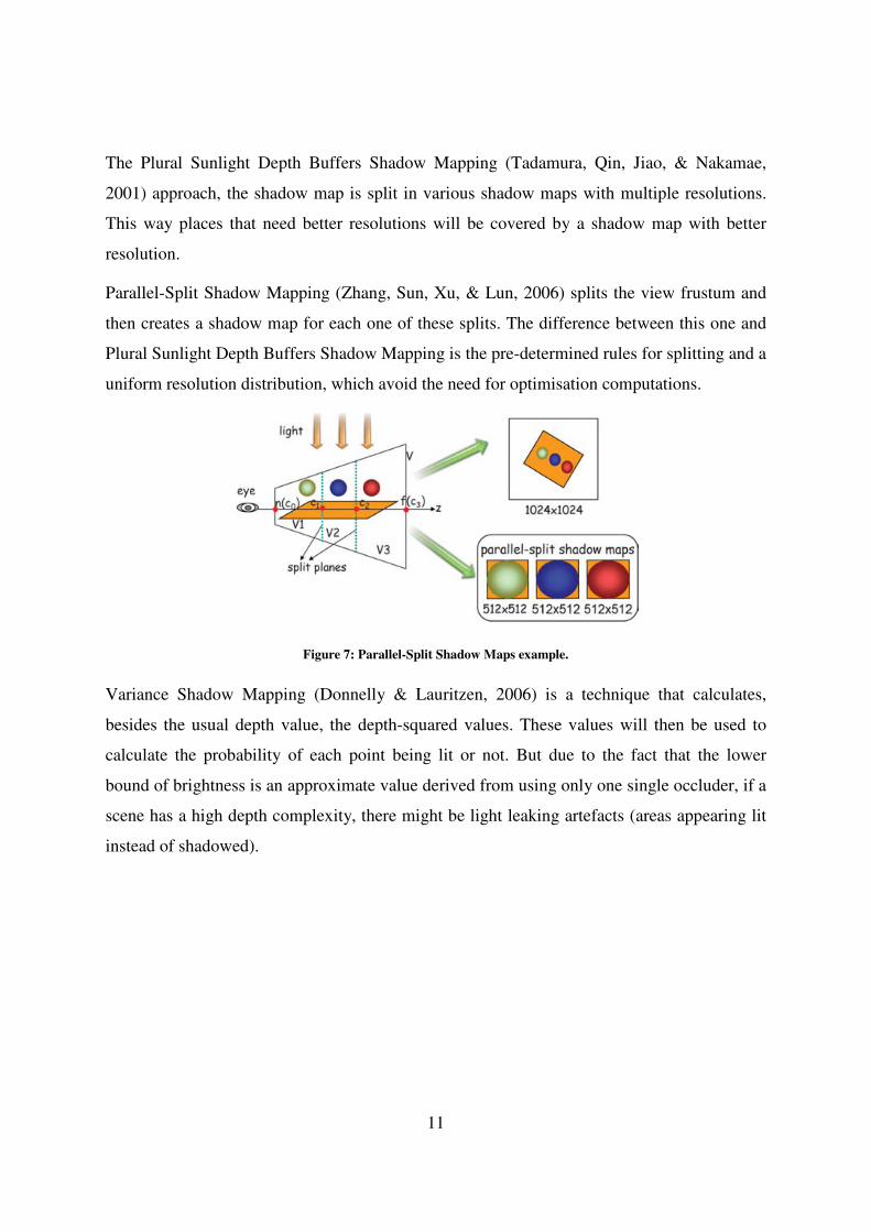
11
The Plural Sunlight Depth Buffers Shadow Mapping (Tadamura, Qin, Jiao, & Nakamae,
2001) approach, the shadow map is split in various shadow maps with multiple resolutions.
This way places that need better resolutions will be covered by a shadow map with better
resolution.
Parallel-Split Shadow Mapping (Zhang, Sun, Xu, & Lun, 2006) splits the view frustum and
then creates a shadow map for each one of these splits. The difference between this one and
Plural Sunlight Depth Buffers Shadow Mapping is the pre-determined rules for splitting and a
uniform resolution distribution, which avoid the need for optimisation computations.
Figure 7: Parallel-Split Shadow Maps example.
Variance Shadow Mapping (Donnelly & Lauritzen, 2006) is a technique that calculates,
besides the usual depth value, the depth-squared values. These values will then be used to
calculate the probability of each point being lit or not. But due to the fact that the lower
bound of brightness is an approximate value derived from using only one single occluder, if a
scene has a high depth complexity, there might be light leaking artefacts (areas appearing lit
instead of shadowed).
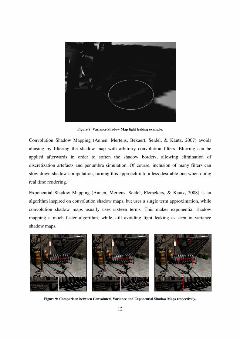
12
Figure 8: Variance Shadow Map light leaking example.
Convolution Shadow Mapping (Annen, Mertens, Bekaert, Seidel, & Kautz, 2007) avoids
aliasing by filtering the shadow map with arbitrary convolution filters. Blurring can be
applied afterwards in order to soften the shadow borders, allowing elimination of
discretization artefacts and penumbra simulation. Of course, inclusion of many filters can
slow down shadow computation, turning this approach into a less desirable one when doing
real time rendering.
Exponential Shadow Mapping (Annen, Mertens, Seidel, Flerackers, & Kautz, 2008) is an
algorithm inspired on convolution shadow maps, but uses a single term approximation, while
convolution shadow maps usually uses sixteen terms. This makes exponential shadow
mapping a much faster algorithm, while still avoiding light leaking as seen in variance
shadow maps.
Figure 9: Comparison between Convoluted, Variance and Exponential Shadow Maps respectively.
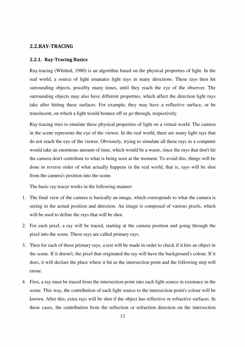
13
2.2. RAY-TRACING
2.2.1. Ray-Tracing Basics
Ray-tracing (Whitted, 1980) is an algorithm based on the physical properties of light. In the
real world, a source of light emanates light rays in many directions. These rays then hit
surrounding objects, possibly many times, until they reach the eye of the observer. The
surrounding objects may also have different properties, which affect the direction light rays
take after hitting these surfaces. For example, they may have a reflective surface, or be
translucent, on which a light would bounce off or go through, respectively.
Ray-tracing tries to emulate these physical properties of light on a virtual world. The camera
in the scene represents the eye of the viewer. In the real world, there are many light rays that
do not reach the eye of the viewer. Obviously, trying to simulate all these rays in a computer
would take an enormous amount of time, which would be a waste, since the rays that don't hit
the camera don't contribute to what is being seen at the moment. To avoid this, things will be
done in reverse order of what actually happens in the real world, that is, rays will be shot
from the camera's position into the scene.
The basic ray-tracer works in the following manner:
1. The final view of the camera is basically an image, which corresponds to what the camera is
seeing in the actual position and direction. An image is composed of various pixels, which
will be used to define the rays that will be shot.
2. For each pixel, a ray will be traced, starting at the camera position and going through the
pixel into the scene. These rays are called primary rays.
3. Then for each of these primary rays, a test will be made in order to check if it hits an object in
the scene. If it doesn't, the pixel that originated the ray will have the background's colour. If it
does, it will declare the place where it hit as the intersection point and the following step will
ensue.
4. First, a ray must be traced from the intersection point into each light source in existence in the
scene. This way, the contribution of each light source to the intersection point's colour will be
known. After this, extra rays will be shot if the object has reflective or refractive surfaces. In
these cases, the contribution from the reflection or refraction direction on the intersection
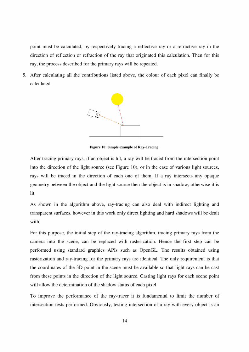
14
point must be calculated, by respectively tracing a reflective ray or a refractive ray in the
direction of reflection or refraction of the ray that originated this calculation. Then for this
ray, the process described for the primary rays will be repeated.
5. After calculating all the contributions listed above, the colour of each pixel can finally be
calculated.
Figure 10: Simple example of Ray-Tracing.
After tracing primary rays, if an object is hit, a ray will be traced from the intersection point
into the direction of the light source (see Figure 10), or in the case of various light sources,
rays will be traced in the direction of each one of them. If a ray intersects any opaque
geometry between the object and the light source then the object is in shadow, otherwise it is
lit.
As shown in the algorithm above, ray-tracing can also deal with indirect lighting and
transparent surfaces, however in this work only direct lighting and hard shadows will be dealt
with.
For this purpose, the initial step of the ray-tracing algorithm, tracing primary rays from the
camera into the scene, can be replaced with rasterization. Hence the first step can be
performed using standard graphics APIs such as OpenGL. The results obtained using
rasterization and ray-tracing for the primary rays are identical. The only requirement is that
the coordinates of the 3D point in the scene must be available so that light rays can be cast
from these points in the direction of the light source. Casting light rays for each scene point
will allow the determination of the shadow status of each pixel.
To improve the performance of the ray-tracer it is fundamental to limit the number of
intersection tests performed. Obviously, testing intersection of a ray with every object is an
15
enormous waste of time, because most objects would probably not be intersected, hence
being redundant to the final result. One way to achieve a more rational selection of geometry
to intersect is to use hierarchic bounding volumes or spatial partitioning. Under these
approaches, various objects will be grouped together in a bounding volume. Checking for
intersections is done first with the bounding volume itself, and only if an intersection with the
volume exists will the geometry inside be tested. If the ray doesn't intersect the bounding
volume, it obviously won't intersect any of the objects within it. A hierarchy of bounding
volumes will potentially accelerate the process even further. The most common bounding
volumes are the bounding spheres and bounding boxes, which are simple polygons and allow
for quick intersection tests. Examples of spatial subdivision include octrees, binary space
partitioning (BSP), kD-trees and grids.
2.3. COMBINING BOTH
As seen before shadow mapping is a very efficient algorithm performance wise, yet it is
prone to all sorts of aliasing errors, producing shadows containing a large number of
artefacts. On the other hand ray-tracing is capable of producing pixel perfect shadows at the
expense of a mode computational expensive algorithm.
Some researchers have attempted to combine both the performance of the shadow mapping
algorithm and the accuracy of the ray-tracer solution.
The common approach behind these methods starts by first computing a shadow map. Ray-
tracing is then used selectively for particular pixels that are classified as having an unreliable
shadow status.
This greatly reduces the number of rays, and as a consequence the number of intersections to
be performed. The results clearly show great improvements when comparing to the shadow
map initial result, while still being far lighter than an exclusive ray-tracing solution.
2.3.1. Coherence-Based Ray-Tracing
The Coherence-Based Ray-Tracing (Agrawala, Ramamoorthi, Heirich, & Moll, 2000)
algorithm combines a hierarchical ray-tracing technique and a coherence-based sampling
technique in order to create soft shadows from area light sources. It starts by creating various
reference images from various locations in the scene and saves object depths the same way
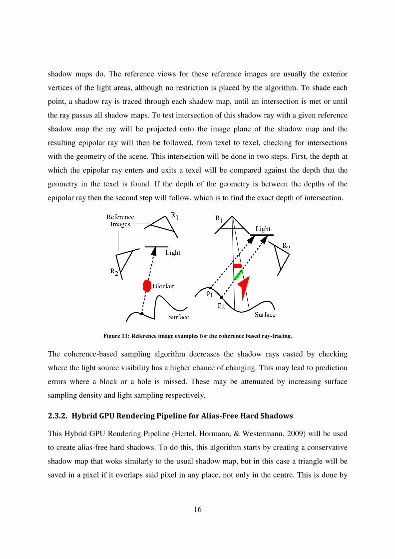
16
shadow maps do. The reference views for these reference images are usually the exterior
vertices of the light areas, although no restriction is placed by the algorithm. To shade each
point, a shadow ray is traced through each shadow map, until an intersection is met or until
the ray passes all shadow maps. To test intersection of this shadow ray with a given reference
shadow map the ray will be projected onto the image plane of the shadow map and the
resulting epipolar ray will then be followed, from texel to texel, checking for intersections
with the geometry of the scene. This intersection will be done in two steps. First, the depth at
which the epipolar ray enters and exits a texel will be compared against the depth that the
geometry in the texel is found. If the depth of the geometry is between the depths of the
epipolar ray then the second step will follow, which is to find the exact depth of intersection.
Figure 11: Reference image examples for the coherence based ray-tracing.
The coherence-based sampling algorithm decreases the shadow rays casted by checking
where the light source visibility has a higher chance of changing. This may lead to prediction
errors where a block or a hole is missed. These may be attenuated by increasing surface
sampling density and light sampling respectively,
2.3.2. Hybrid GPU Rendering Pipeline for Alias-Free Hard Shadows
This Hybrid GPU Rendering Pipeline (Hertel, Hormann, & Westermann, 2009) will be used
to create alias-free hard shadows. To do this, this algorithm starts by creating a conservative
shadow map that woks similarly to the usual shadow map, but in this case a triangle will be
saved in a pixel if it overlaps said pixel in any place, not only in the centre. This is done by
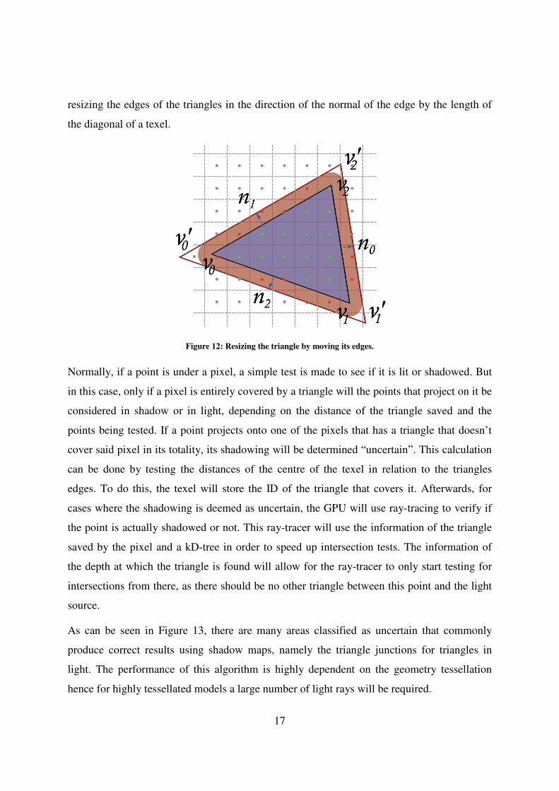
17
resizing the edges of the triangles in the direction of the normal of the edge by the length of
the diagonal of a texel.
Figure 12: Resizing the triangle by moving its edges.
Normally, if a point is under a pixel, a simple test is made to see if it is lit or shadowed. But
in this case, only if a pixel is entirely covered by a triangle will the points that project on it be
considered in shadow or in light, depending on the distance of the triangle saved and the
points being tested. If a point projects onto one of the pixels that has a triangle that doesn’t
cover said pixel in its totality, its shadowing will be determined “uncertain”. This calculation
can be done by testing the distances of the centre of the texel in relation to the triangles
edges. To do this, the texel will store the ID of the triangle that covers it. Afterwards, for
cases where the shadowing is deemed as uncertain, the GPU will use ray-tracing to verify if
the point is actually shadowed or not. This ray-tracer will use the information of the triangle
saved by the pixel and a kD-tree in order to speed up intersection tests. The information of
the depth at which the triangle is found will allow for the ray-tracer to only start testing for
intersections from there, as there should be no other triangle between this point and the light
source.
As can be seen in Figure 13, there are many areas classified as uncertain that commonly
produce correct results using shadow maps, namely the triangle junctions for triangles in
light. The performance of this algorithm is highly dependent on the geometry tessellation
hence for highly tessellated models a large number of light rays will be required.
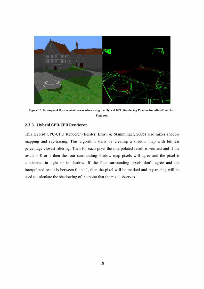
18
Figure 13: Example of the uncertain areas when using the Hybrid GPU Rendering Pipeline for Alias-Free Hard
Shadows.
2.3.3. Hybrid GPU-CPU Renderer
This Hybrid GPU-CPU Renderer (Beister, Ernst, & Stamminger, 2005) also mixes shadow
mapping and ray-tracing. This algorithm starts by creating a shadow map with bilinear
percentage closest filtering. Then for each pixel the interpolated result is verified and if the
result is 0 or 1 then the four surrounding shadow map pixels will agree and the pixel is
considered in light or in shadow. If the four surrounding pixels don’t agree and the
interpolated result is between 0 and 1, then the pixel will be marked and ray-tracing will be
used to calculate the shadowing of the point that the pixel observes.
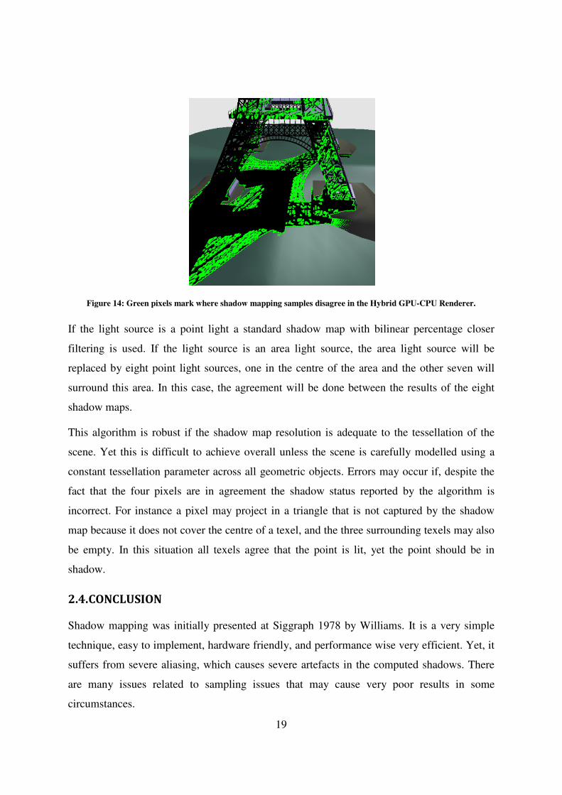
19
Figure 14: Green pixels mark where shadow mapping samples disagree in the Hybrid GPU-CPU Renderer.
If the light source is a point light a standard shadow map with bilinear percentage closer
filtering is used. If the light source is an area light source, the area light source will be
replaced by eight point light sources, one in the centre of the area and the other seven will
surround this area. In this case, the agreement will be done between the results of the eight
shadow maps.
This algorithm is robust if the shadow map resolution is adequate to the tessellation of the
scene. Yet this is difficult to achieve overall unless the scene is carefully modelled using a
constant tessellation parameter across all geometric objects. Errors may occur if, despite the
fact that the four pixels are in agreement the shadow status reported by the algorithm is
incorrect. For instance a pixel may project in a triangle that is not captured by the shadow
map because it does not cover the centre of a texel, and the three surrounding texels may also
be empty. In this situation all texels agree that the point is lit, yet the point should be in
shadow.
2.4. CONCLUSION
Shadow mapping was initially presented at Siggraph 1978 by Williams. It is a very simple
technique, easy to implement, hardware friendly, and performance wise very efficient. Yet, it
suffers from severe aliasing, which causes severe artefacts in the computed shadows. There
are many issues related to sampling issues that may cause very poor results in some
circumstances.
20
The perspective mismatch and projection issues, together with limited hardware precision
gave rise to a lot of research to improve this algorithm. Several methods are based on the
computation of the light frustum to improve the texel usage of the shadow map. Others such
as Cascade Shadow Maps propose the computation of a set of shadow maps to cope with the
under-sampling issue. Algorithms such as Perspective Shadow Mapping and Light Image
Space Shadow Mapping transform the projection itself to deal with the same issue.
These methods have produced great improvements on the shadow mapping result, producing
shadows far more perfect than the original algorithm, without significantly overloading the
algorithm performance wise.
The ray-tracing approach is far more capable quality wise, producing pixel perfect shadows.
However it requires a much larger number of computations, hence it is computationally more
expensive than shadow mapping.
Researchers have combined both methods, in an attempt to get the performance of the
shadow map algorithm, and the accuracy of the ray-tracer solution. These approaches initially
compute a shadow map and then perform selective ray-tracing for a comparatively small
number of pixels.
Although the results are far superior to the standard algorithm, all solutions above are not
error free.
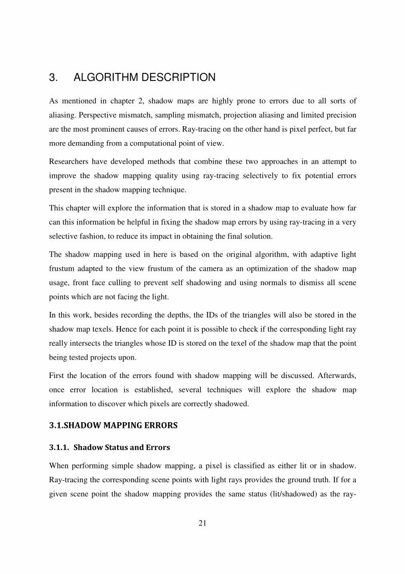
21
3. ALGORITHM DESCRIPTION
As mentioned in chapter 2, shadow maps are highly prone to errors due to all sorts of
aliasing. Perspective mismatch, sampling mismatch, projection aliasing and limited precision
are the most prominent causes of errors. Ray-tracing on the other hand is pixel perfect, but far
more demanding from a computational point of view.
Researchers have developed methods that combine these two approaches in an attempt to
improve the shadow mapping quality using ray-tracing selectively to fix potential errors
present in the shadow mapping technique.
This chapter will explore the information that is stored in a shadow map to evaluate how far
can this information be helpful in fixing the shadow map errors by using ray-tracing in a very
selective fashion, to reduce its impact in obtaining the final solution.
The shadow mapping used in here is based on the original algorithm, with adaptive light
frustum adapted to the view frustum of the camera as an optimization of the shadow map
usage, front face culling to prevent self shadowing and using normals to dismiss all scene
points which are not facing the light.
In this work, besides recording the depths, the IDs of the triangles will also be stored in the
shadow map texels. Hence for each point it is possible to check if the corresponding light ray
really intersects the triangles whose ID is stored on the texel of the shadow map that the point
being tested projects upon.
First the location of the errors found with shadow mapping will be discussed. Afterwards,
once error location is established, several techniques will explore the shadow map
information to discover which pixels are correctly shadowed.
3.1. SHADOW MAPPING ERRORS
3.1.1. Shadow Status and Errors
When performing simple shadow mapping, a pixel is classified as either lit or in shadow.
Ray-tracing the corresponding scene points with light rays provides the ground truth. If for a
given scene point the shadow mapping provides the same status (lit/shadowed) as the ray-
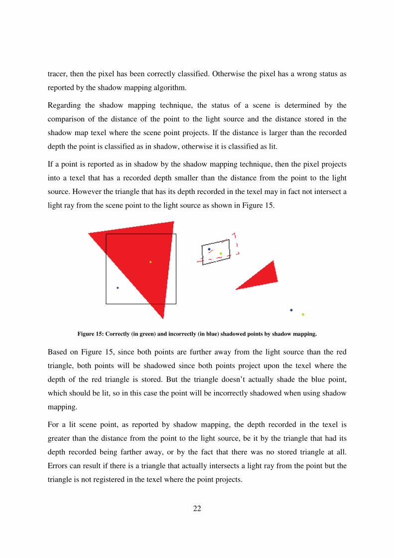
22
tracer, then the pixel has been correctly classified. Otherwise the pixel has a wrong status as
reported by the shadow mapping algorithm.
Regarding the shadow mapping technique, the status of a scene is determined by the
comparison of the distance of the point to the light source and the distance stored in the
shadow map texel where the scene point projects. If the distance is larger than the recorded
depth the point is classified as in shadow, otherwise it is classified as lit.
If a point is reported as in shadow by the shadow mapping technique, then the pixel projects
into a texel that has a recorded depth smaller than the distance from the point to the light
source. However the triangle that has its depth recorded in the texel may in fact not intersect a
light ray from the scene point to the light source as shown in Figure 15.
Figure 15: Correctly (in green) and incorrectly (in blue) shadowed points by shadow mapping.
Based on Figure 15, since both points are further away from the light source than the red
triangle, both points will be shadowed since both points project upon the texel where the
depth of the red triangle is stored. But the triangle doesn’t actually shade the blue point,
which should be lit, so in this case the point will be incorrectly shadowed when using shadow
mapping.
For a lit scene point, as reported by shadow mapping, the depth recorded in the texel is
greater than the distance from the point to the light source, be it by the triangle that had its
depth recorded being farther away, or by the fact that there was no stored triangle at all.
Errors can result if there is a triangle that actually intersects a light ray from the point but the
triangle is not registered in the texel where the point projects.
23
Figure 16: Correctly (in green) and incorrectly (in blue) lit points by shadow mapping.
In Figure 16, the depth stored in the texel is the maximum value possible since there is no
triangle that projects upon its centre. Since the depth stored is higher than the depth of the
two points, both will be lit when using shadow mapping. But the blue point has another
triangle, the red one, which shades it. But as the depth of this triangle isn’t stored in the texel,
since the triangle doesn’t cover the centre of the texel, it won’t be able to shadow the point.
The same would happen if the stored depth came from a triangle further away than the points
being tested.
3.1.2. Error Location
A naked eye comparison between shadow mapping and ray-tracer solutions shows that
shadow mapping errors are mostly present in the contours. This can be observed in Figure 17.
Figure 17 marks the contours in green, the errors inside the contours in red if the pixel is
incorrectly lit and in yellow if the pixel is incorrectly shadowed and in blue if the error is
outside the contour. The larger the width of the contour line the more errors are contained in
the contour. To create an unbiased contour, i.e. a contour that has roughly 50/50 shadow/light
pixels a contour with an even width is used.
The resolution of the shadow map plays a crucial role in the percentage of errors caught in
the contours. Higher resolutions have a better definition of the shadowed areas hence require
narrower contours, whereas lower resolutions need thicker contour lines to catch a similar
percentage of errors.
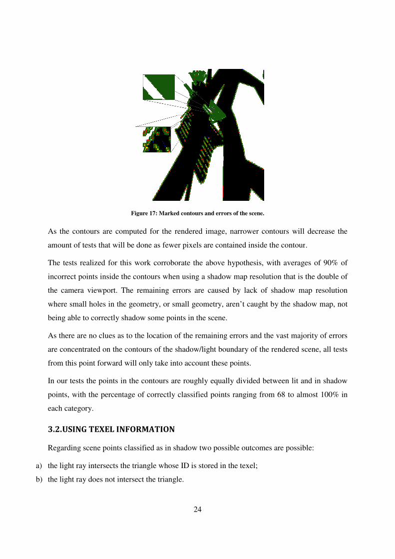
Figure
As the contours are computed for the rendered image, narrower contour
amount of tests that will be done
The tests realized for this work corroborate the above hypothesis
incorrect points inside the contours
the camera viewport. The remaining
where small holes in the geometry
being able to correctly shadow some points in the scene.
As there are no clues as to the location of the remaining errors
are concentrated on the contours of the shadow/light boundary of the rendered scene, all tests
from this point forward will only
In our tests the points in the contours are roughly equally divided between lit and in shadow
points, with the percentage of correctly classified points ranging from 68 to almost 100% in
each category.
3.2. USING TEXEL INFORMAT
Regarding scene points classified as in shadow
a) the light ray intersects the triangle
b) the light ray does not intersect the triangle.
24
Figure 17: Marked contours and errors of the scene.
As the contours are computed for the rendered image, narrower contour
amount of tests that will be done as fewer pixels are contained inside the contour
this work corroborate the above hypothesis, with averages of 90% of
incorrect points inside the contours when using a shadow map resolution that is the double of
remaining errors are caused by lack of shadow map resolution
all holes in the geometry, or small geometry, aren’t caught by the shadow map, not
shadow some points in the scene.
there are no clues as to the location of the remaining errors and the vast majority of errors
the contours of the shadow/light boundary of the rendered scene, all tests
only take into account these points.
In our tests the points in the contours are roughly equally divided between lit and in shadow
centage of correctly classified points ranging from 68 to almost 100% in
USING TEXEL INFORMATION
points classified as in shadow two possible outcomes are possible:
the light ray intersects the triangle whose ID is stored in the texel;
the light ray does not intersect the triangle.
As the contours are computed for the rendered image, narrower contours will decrease the
contour.
, with averages of 90% of
when using a shadow map resolution that is the double of
y lack of shadow map resolution
n’t caught by the shadow map, not
the vast majority of errors
the contours of the shadow/light boundary of the rendered scene, all tests
In our tests the points in the contours are roughly equally divided between lit and in shadow
centage of correctly classified points ranging from 68 to almost 100% in
two possible outcomes are possible:
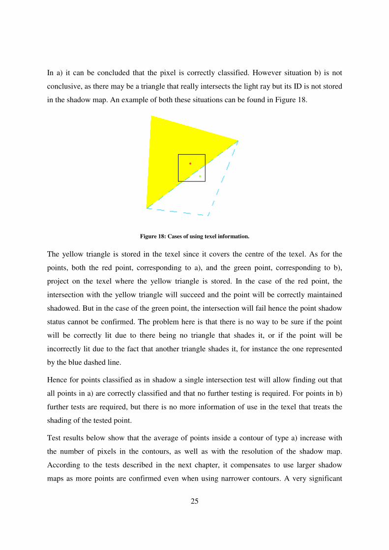
25
In a) it can be concluded that the pixel is correctly classified. However situation b) is not
conclusive, as there may be a triangle that really intersects the light ray but its ID is not stored
in the shadow map. An example of both these situations can be found in Figure 18.
Figure 18: Cases of using texel information.
The yellow triangle is stored in the texel since it covers the centre of the texel. As for the
points, both the red point, corresponding to a), and the green point, corresponding to b),
project on the texel where the yellow triangle is stored. In the case of the red point, the
intersection with the yellow triangle will succeed and the point will be correctly maintained
shadowed. But in the case of the green point, the intersection will fail hence the point shadow
status cannot be confirmed. The problem here is that there is no way to be sure if the point
will be correctly lit due to there being no triangle that shades it, or if the point will be
incorrectly lit due to the fact that another triangle shades it, for instance the one represented
by the blue dashed line.
Hence for points classified as in shadow a single intersection test will allow finding out that
all points in a) are correctly classified and that no further testing is required. For points in b)
further tests are required, but there is no more information of use in the texel that treats the
shading of the tested point.
Test results below show that the average of points inside a contour of type a) increase with
the number of pixels in the contours, as well as with the resolution of the shadow map.
According to the tests described in the next chapter, it compensates to use larger shadow
maps as more points are confirmed even when using narrower contours. A very significant
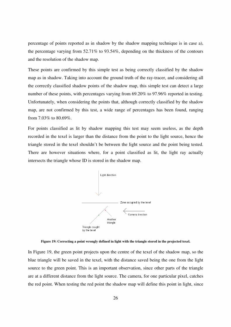
26
percentage of points reported as in shadow by the shadow mapping technique is in case a),
the percentage varying from 52.71% to 93.54%, depending on the thickness of the contours
and the resolution of the shadow map.
These points are confirmed by this simple test as being correctly classified by the shadow
map as in shadow. Taking into account the ground truth of the ray-tracer, and considering all
the correctly classified shadow points of the shadow map, this simple test can detect a large
number of these points, with percentages varying from 69.20% to 97.96% reported in testing.
Unfortunately, when considering the points that, although correctly classified by the shadow
map, are not confirmed by this test, a wide range of percentages has been found, ranging
from 7.03% to 80.69%.
For points classified as lit by shadow mapping this test may seem useless, as the depth
recorded in the texel is larger than the distance from the point to the light source, hence the
triangle stored in the texel shouldn’t be between the light source and the point being tested.
There are however situations where, for a point classified as lit, the light ray actually
intersects the triangle whose ID is stored in the shadow map.
Figure 19: Correcting a point wrongly defined in light with the triangle stored in the projected texel.
In Figure 19, the green point projects upon the centre of the texel of the shadow map, so the
blue triangle will be saved in the texel, with the distance saved being the one from the light
source to the green point. This is an important observation, since other parts of the triangle
are at a different distance from the light source. The camera, for one particular pixel, catches
the red point. When testing the red point the shadow map will define this point in light, since
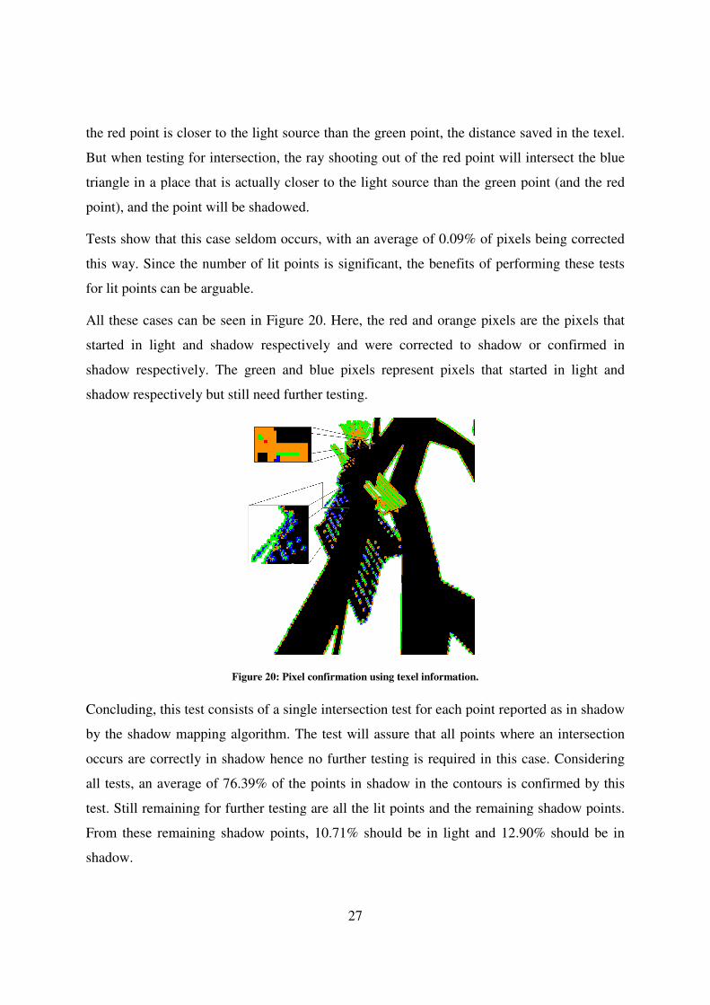
the red point is closer to the light source than the green point, the distance saved
But when testing for intersection, the ray shooting out of the red point will intersect the blue
triangle in a place that is actually closer to the light source t
point), and the point will be shadowed.
Tests show that this case seldom occurs
this way. Since the number of lit points is significant, the benefits of performing these t
for lit points can be arguable.
All these cases can be seen in
started in light and shadow respectively and were corrected to shadow or confirmed in
shadow respectively. The green and blue pixels repre
shadow respectively but still need further testing.
Figure
Concluding, this test consists of a single intersection test for each point
by the shadow mapping algorithm
occurs are correctly in shadow
all tests, an average of 76.39% of the points in shadow in the contours
test. Still remaining for further testing are all the lit points and the remaining shadow points.
From these remaining shadow points, 10.71% should be in light and 12.90% should be in
shadow.
27
ed point is closer to the light source than the green point, the distance saved
But when testing for intersection, the ray shooting out of the red point will intersect the blue
triangle in a place that is actually closer to the light source than the green point (and the red
and the point will be shadowed.
ow that this case seldom occurs, with an average of 0.09% of pixels being corrected
. Since the number of lit points is significant, the benefits of performing these t
.
All these cases can be seen in Figure 20. Here, the red and orange pixels are the pixels that
started in light and shadow respectively and were corrected to shadow or confirmed in
shadow respectively. The green and blue pixels represent pixels that started in light and
shadow respectively but still need further testing.
Figure 20: Pixel confirmation using texel information.
Concluding, this test consists of a single intersection test for each point reported
by the shadow mapping algorithm. The test will assure that all points where an intersection
shadow hence no further testing is required in this case.
% of the points in shadow in the contours is
Still remaining for further testing are all the lit points and the remaining shadow points.
From these remaining shadow points, 10.71% should be in light and 12.90% should be in
ed point is closer to the light source than the green point, the distance saved in the texel.
But when testing for intersection, the ray shooting out of the red point will intersect the blue
han the green point (and the red
with an average of 0.09% of pixels being corrected
. Since the number of lit points is significant, the benefits of performing these tests
. Here, the red and orange pixels are the pixels that
started in light and shadow respectively and were corrected to shadow or confirmed in
sent pixels that started in light and
reported as in shadow
. The test will assure that all points where an intersection
hence no further testing is required in this case. Considering
is confirmed by this
Still remaining for further testing are all the lit points and the remaining shadow points.
From these remaining shadow points, 10.71% should be in light and 12.90% should be in
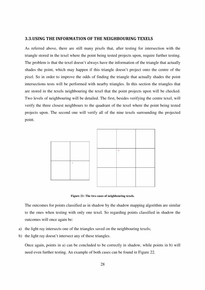
28
3.3. USING THE INFORMATION OF THE NEIGHBOURING TEXELS
As referred above, there are still many pixels that, after testing for intersection with the
triangle stored in the texel where the point being tested projects upon, require further testing.
The problem is that the texel doesn’t always have the information of the triangle that actually
shades the point, which may happen if this triangle doesn’t project onto the centre of the
pixel. So in order to improve the odds of finding the triangle that actually shades the point
intersections tests will be performed with nearby triangles. In this section the triangles that
are stored in the texels neighbouring the texel that the point projects upon will be checked.
Two levels of neighbouring will be detailed. The first, besides verifying the centre texel, will
verify the three closest neighbours to the quadrant of the texel where the point being tested
projects upon. The second one will verify all of the nine texels surrounding the projected
point.
Figure 21: The two cases of neighbouring texels.
The outcomes for points classified as in shadow by the shadow mapping algorithm are similar
to the ones when testing with only one texel. So regarding points classified in shadow the
outcomes will once again be:
a) the light ray intersects one of the triangles saved on the neighbouring texels;
b) the light ray doesn’t intersect any of these triangles.
Once again, points in a) can be concluded to be correctly in shadow, while points in b) will
need even further testing. An example of both cases can be found in Figure 22.
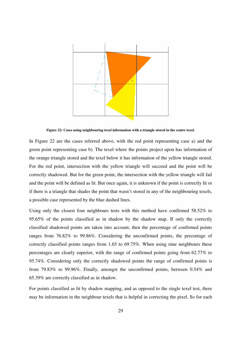
29
Figure 22: Cases using neighbouring texel information with a triangle stored in the centre texel.
In Figure 22 are the cases referred above, with the red point representing case a) and the
green point representing case b). The texel where the points project upon has information of
the orange triangle stored and the texel below it has information of the yellow triangle stored.
For the red point, intersection with the yellow triangle will succeed and the point will be
correctly shadowed. But for the green point, the intersection with the yellow triangle will fail
and the point will be defined as lit. But once again, it is unknown if the point is correctly lit or
if there is a triangle that shades the point that wasn’t stored in any of the neighbouring texels,
a possible case represented by the blue dashed lines.
Using only the closest four neighbours tests with this method have confirmed 58.52% to
95.65% of the points classified as in shadow by the shadow map. If only the correctly
classified shadowed points are taken into account, then the percentage of confirmed points
ranges from 76.82% to 99.86%. Considering the unconfirmed points, the percentage of
correctly classified points ranges from 1.65 to 69.75%. When using nine neighbours these
percentages are clearly superior, with the range of confirmed points going from 62.77% to
95.74%. Considering only the correctly shadowed points the range of confirmed points is
from 79.83% to 99.96%. Finally, amongst the unconfirmed points, between 0.54% and
65.39% are correctly classified as in shadow.
For points classified as lit by shadow mapping, and as opposed to the single texel test, there
may be information in the neighbour texels that is helpful in correcting the pixel. So for each
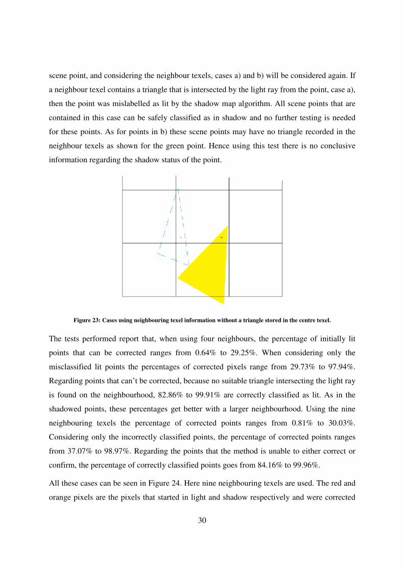
30
scene point, and considering the neighbour texels, cases a) and b) will be considered again. If
a neighbour texel contains a triangle that is intersected by the light ray from the point, case a),
then the point was mislabelled as lit by the shadow map algorithm. All scene points that are
contained in this case can be safely classified as in shadow and no further testing is needed
for these points. As for points in b) these scene points may have no triangle recorded in the
neighbour texels as shown for the green point. Hence using this test there is no conclusive
information regarding the shadow status of the point.
Figure 23: Cases using neighbouring texel information without a triangle stored in the centre texel.
The tests performed report that, when using four neighbours, the percentage of initially lit
points that can be corrected ranges from 0.64% to 29.25%. When considering only the
misclassified lit points the percentages of corrected pixels range from 29.73% to 97.94%.
Regarding points that can’t be corrected, because no suitable triangle intersecting the light ray
is found on the neighbourhood, 82.86% to 99.91% are correctly classified as lit. As in the
shadowed points, these percentages get better with a larger neighbourhood. Using the nine
neighbouring texels the percentage of corrected points ranges from 0.81% to 30.03%.
Considering only the incorrectly classified points, the percentage of corrected points ranges
from 37.07% to 98.97%. Regarding the points that the method is unable to either correct or
confirm, the percentage of correctly classified points goes from 84.16% to 99.96%.
All these cases can be seen in Figure 24. Here nine neighbouring texels are used. The red and
orange pixels are the pixels that started in light and shadow respectively and were corrected
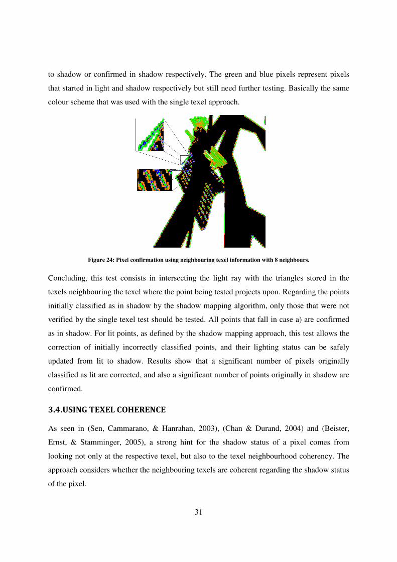
to shadow or confirmed in shadow respectively. The green and blue pixels represent pixels
that started in light and shadow respectively but still need further testing. Basically the same
colour scheme that was used with the single texel approach.
Figure 24: Pixel confirmation using neighbouring texel information
Concluding, this test consists in intersecting the
texels neighbouring the texel where the point being tested projects
initially classified as in shadow by the shadow mapping algorithm, only those that were not
verified by the single texel test should be tested
as in shadow. For lit points, as define
correction of initially incorrectly classified points, and their lighting status
updated from lit to shadow. Results show that a significant number of pixels originally
classified as lit are corrected, and also a significant number of points originally in shadow are
confirmed.
3.4. USING TEXEL COHERENC
As seen in (Sen, Cammarano, & Hanrahan, 2003)
Ernst, & Stamminger, 2005)
looking not only at the respective texel, but also to th
approach considers whether the neighbo
of the pixel.
31
or confirmed in shadow respectively. The green and blue pixels represent pixels
that started in light and shadow respectively but still need further testing. Basically the same
colour scheme that was used with the single texel approach.
: Pixel confirmation using neighbouring texel information with 8 neighbours
Concluding, this test consists in intersecting the light ray with the triangles stored in the
texels neighbouring the texel where the point being tested projects upon. Regarding the points
initially classified as in shadow by the shadow mapping algorithm, only those that were not
verified by the single texel test should be tested. All points that fall in case a) are confirmed
as in shadow. For lit points, as defined by the shadow mapping approach, this test allows the
initially incorrectly classified points, and their lighting status
lit to shadow. Results show that a significant number of pixels originally
are corrected, and also a significant number of points originally in shadow are
USING TEXEL COHERENCE
(Sen, Cammarano, & Hanrahan, 2003), (Chan & Durand, 2004)
Ernst, & Stamminger, 2005), a strong hint for the shadow status of a pixel comes from
looking not only at the respective texel, but also to the texel neighbourhood coherency.
approach considers whether the neighbouring texels are coherent regarding the shadow status
or confirmed in shadow respectively. The green and blue pixels represent pixels
that started in light and shadow respectively but still need further testing. Basically the same
with 8 neighbours.
triangles stored in the
Regarding the points
initially classified as in shadow by the shadow mapping algorithm, only those that were not
All points that fall in case a) are confirmed
d by the shadow mapping approach, this test allows the
initially incorrectly classified points, and their lighting status can be safely
lit to shadow. Results show that a significant number of pixels originally
are corrected, and also a significant number of points originally in shadow are
(Chan & Durand, 2004) and (Beister,
strong hint for the shadow status of a pixel comes from
e texel neighbourhood coherency. The
uring texels are coherent regarding the shadow status
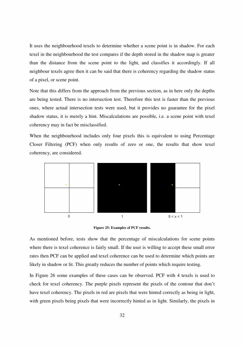
32
It uses the neighbourhood texels to determine whether a scene point is in shadow. For each
texel in the neighbourhood the test compares if the depth stored in the shadow map is greater
than the distance from the scene point to the light, and classifies it accordingly. If all
neighbour texels agree then it can be said that there is coherency regarding the shadow status
of a pixel, or scene point.
Note that this differs from the approach from the previous section, as in here only the depths
are being tested. There is no intersection test. Therefore this test is faster than the previous
ones, where actual intersection tests were used, but it provides no guarantee for the pixel
shadow status, it is merely a hint. Miscalculations are possible, i.e. a scene point with texel
coherency may in fact be misclassified.
When the neighbourhood includes only four pixels this is equivalent to using Percentage
Closer Filtering (PCF) when only results of zero or one, the results that show texel
coherency, are considered.
Figure 25: Examples of PCF results.
As mentioned before, tests show that the percentage of miscalculations for scene points
where there is texel coherence is fairly small. If the user is willing to accept these small error
rates then PCF can be applied and texel coherence can be used to determine which points are
likely in shadow or lit. This greatly reduces the number of points which require testing.
In Figure 26 some examples of these cases can be observed. PCF with 4 texels is used to
check for texel coherency. The purple pixels represent the pixels of the contour that don’t
have texel coherency. The pixels in red are pixels that were hinted correctly as being in light,
with green pixels being pixels that were incorrectly hinted as in light. Similarly, the pixels in
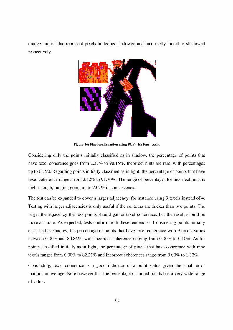
orange and in blue represent pixels
respectively.
Figure
Considering only the points initially classified as in shadow
have texel coherence goes from 2.37% to 90.15%. Incorrect hints are rare, with percentages
up to 0.75%.Regarding points initially classified as in light, the percentage of points that have
texel coherence ranges from 2.42% t
higher tough, ranging going up to 7.07% in some scenes.
The test can be expanded to cover a larger adjacency, for instance using 9 texels instead of 4.
Testing with larger adjacencies is only useful
larger the adjacency the less points should gather texel coherence, but the result should be
more accurate. As expected, tests confirm both these tendencies.
classified as shadow, the percentage of points that have texel coherence with 9 texels varies
between 0.00% and 80.86%, with incorrect coherence ranging from 0.00% to 0.10%. As for
points classified initially as in light, the percentage of pixels that have coherence with nin
texels ranges from 0.00% to 82.27% and incorrect coherences range from 0.00% to 1.32%.
Concluding, texel coherence
margins in average. Note however that the percentage of hinted points has a very wide range
of values.
33
orange and in blue represent pixels hinted as shadowed and incorrectly hint
Figure 26: Pixel confirmation using PCF with four texels.
Considering only the points initially classified as in shadow, the percentage of points that
have texel coherence goes from 2.37% to 90.15%. Incorrect hints are rare, with percentages
up to 0.75%.Regarding points initially classified as in light, the percentage of points that have
texel coherence ranges from 2.42% to 91.70%. The range of percentages for incorrect hints is
higher tough, ranging going up to 7.07% in some scenes.
The test can be expanded to cover a larger adjacency, for instance using 9 texels instead of 4.
Testing with larger adjacencies is only useful if the contours are thicker than two points. The
larger the adjacency the less points should gather texel coherence, but the result should be
more accurate. As expected, tests confirm both these tendencies. Considering points initially
w, the percentage of points that have texel coherence with 9 texels varies
between 0.00% and 80.86%, with incorrect coherence ranging from 0.00% to 0.10%. As for
points classified initially as in light, the percentage of pixels that have coherence with nin
texels ranges from 0.00% to 82.27% and incorrect coherences range from 0.00% to 1.32%.
Concluding, texel coherence is a good indicator of a point status given t
Note however that the percentage of hinted points has a very wide range
hinted as shadowed
, the percentage of points that
have texel coherence goes from 2.37% to 90.15%. Incorrect hints are rare, with percentages
up to 0.75%.Regarding points initially classified as in light, the percentage of points that have
o 91.70%. The range of percentages for incorrect hints is
The test can be expanded to cover a larger adjacency, for instance using 9 texels instead of 4.
if the contours are thicker than two points. The
larger the adjacency the less points should gather texel coherence, but the result should be
Considering points initially
w, the percentage of points that have texel coherence with 9 texels varies
between 0.00% and 80.86%, with incorrect coherence ranging from 0.00% to 0.10%. As for
points classified initially as in light, the percentage of pixels that have coherence with nine
texels ranges from 0.00% to 82.27% and incorrect coherences range from 0.00% to 1.32%.
given the small error
Note however that the percentage of hinted points has a very wide range
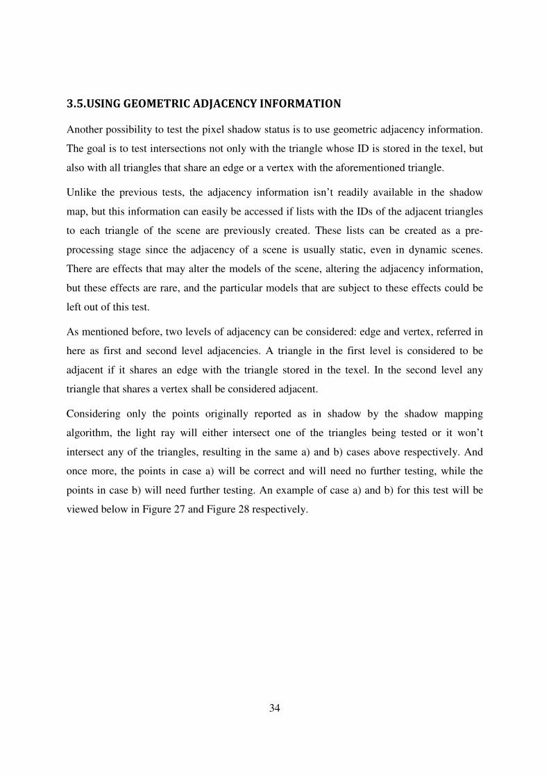
34
3.5. USING GEOMETRIC ADJACENCY INFORMATION
Another possibility to test the pixel shadow status is to use geometric adjacency information.
The goal is to test intersections not only with the triangle whose ID is stored in the texel, but
also with all triangles that share an edge or a vertex with the aforementioned triangle.
Unlike the previous tests, the adjacency information isn’t readily available in the shadow
map, but this information can easily be accessed if lists with the IDs of the adjacent triangles
to each triangle of the scene are previously created. These lists can be created as a pre-
processing stage since the adjacency of a scene is usually static, even in dynamic scenes.
There are effects that may alter the models of the scene, altering the adjacency information,
but these effects are rare, and the particular models that are subject to these effects could be
left out of this test.
As mentioned before, two levels of adjacency can be considered: edge and vertex, referred in
here as first and second level adjacencies. A triangle in the first level is considered to be
adjacent if it shares an edge with the triangle stored in the texel. In the second level any
triangle that shares a vertex shall be considered adjacent.
Considering only the points originally reported as in shadow by the shadow mapping
algorithm, the light ray will either intersect one of the triangles being tested or it won’t
intersect any of the triangles, resulting in the same a) and b) cases above respectively. And
once more, the points in case a) will be correct and will need no further testing, while the
points in case b) will need further testing. An example of case a) and b) for this test will be
viewed below in Figure 27 and Figure 28 respectively.
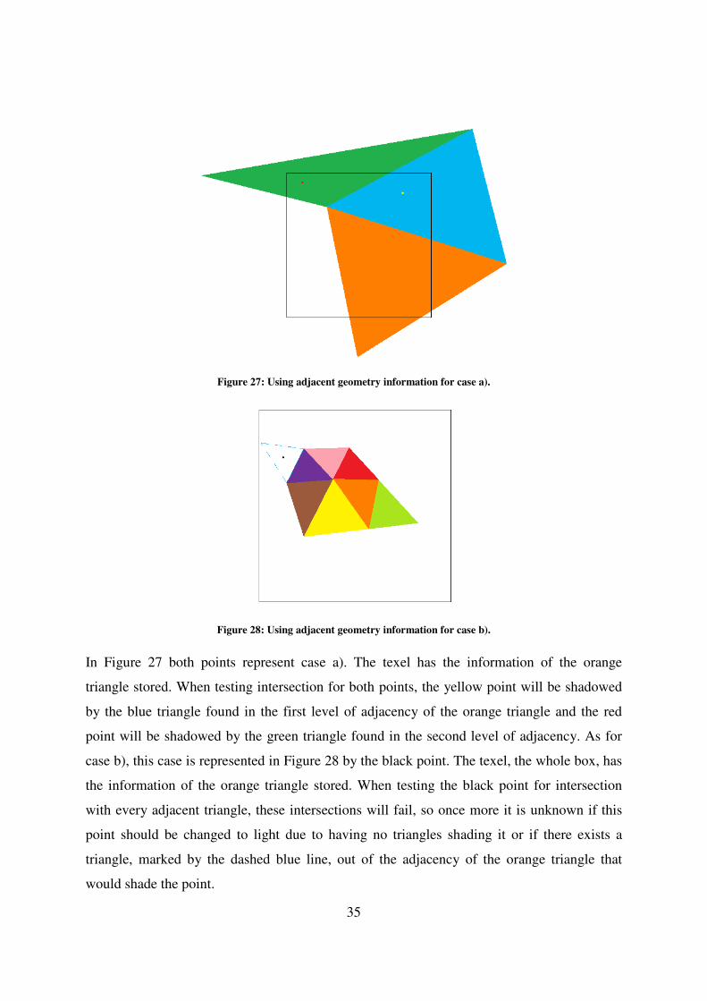
35
Figure 27: Using adjacent geometry information for case a).
Figure 28: Using adjacent geometry information for case b).
In Figure 27 both points represent case a). The texel has the information of the orange
triangle stored. When testing intersection for both points, the yellow point will be shadowed
by the blue triangle found in the first level of adjacency of the orange triangle and the red
point will be shadowed by the green triangle found in the second level of adjacency. As for
case b), this case is represented in Figure 28 by the black point. The texel, the whole box, has
the information of the orange triangle stored. When testing the black point for intersection
with every adjacent triangle, these intersections will fail, so once more it is unknown if this
point should be changed to light due to having no triangles shading it or if there exists a
triangle, marked by the dashed blue line, out of the adjacency of the orange triangle that
would shade the point.
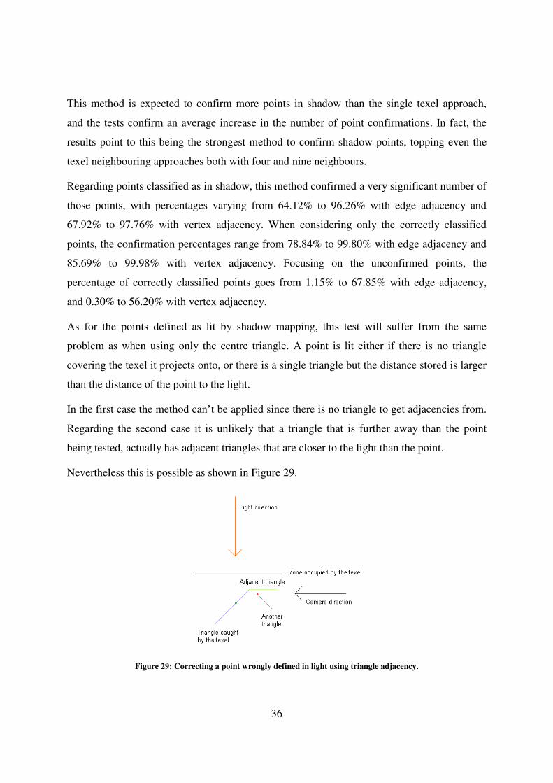
36
This method is expected to confirm more points in shadow than the single texel approach,
and the tests confirm an average increase in the number of point confirmations. In fact, the
results point to this being the strongest method to confirm shadow points, topping even the
texel neighbouring approaches both with four and nine neighbours.
Regarding points classified as in shadow, this method confirmed a very significant number of
those points, with percentages varying from 64.12% to 96.26% with edge adjacency and
67.92% to 97.76% with vertex adjacency. When considering only the correctly classified
points, the confirmation percentages range from 78.84% to 99.80% with edge adjacency and
85.69% to 99.98% with vertex adjacency. Focusing on the unconfirmed points, the
percentage of correctly classified points goes from 1.15% to 67.85% with edge adjacency,
and 0.30% to 56.20% with vertex adjacency.
As for the points defined as lit by shadow mapping, this test will suffer from the same
problem as when using only the centre triangle. A point is lit either if there is no triangle
covering the texel it projects onto, or there is a single triangle but the distance stored is larger
than the distance of the point to the light.
In the first case the method can’t be applied since there is no triangle to get adjacencies from.
Regarding the second case it is unlikely that a triangle that is further away than the point
being tested, actually has adjacent triangles that are closer to the light than the point.
Nevertheless this is possible as shown in Figure 29.
Figure 29: Correcting a point wrongly defined in light using triangle adjacency.
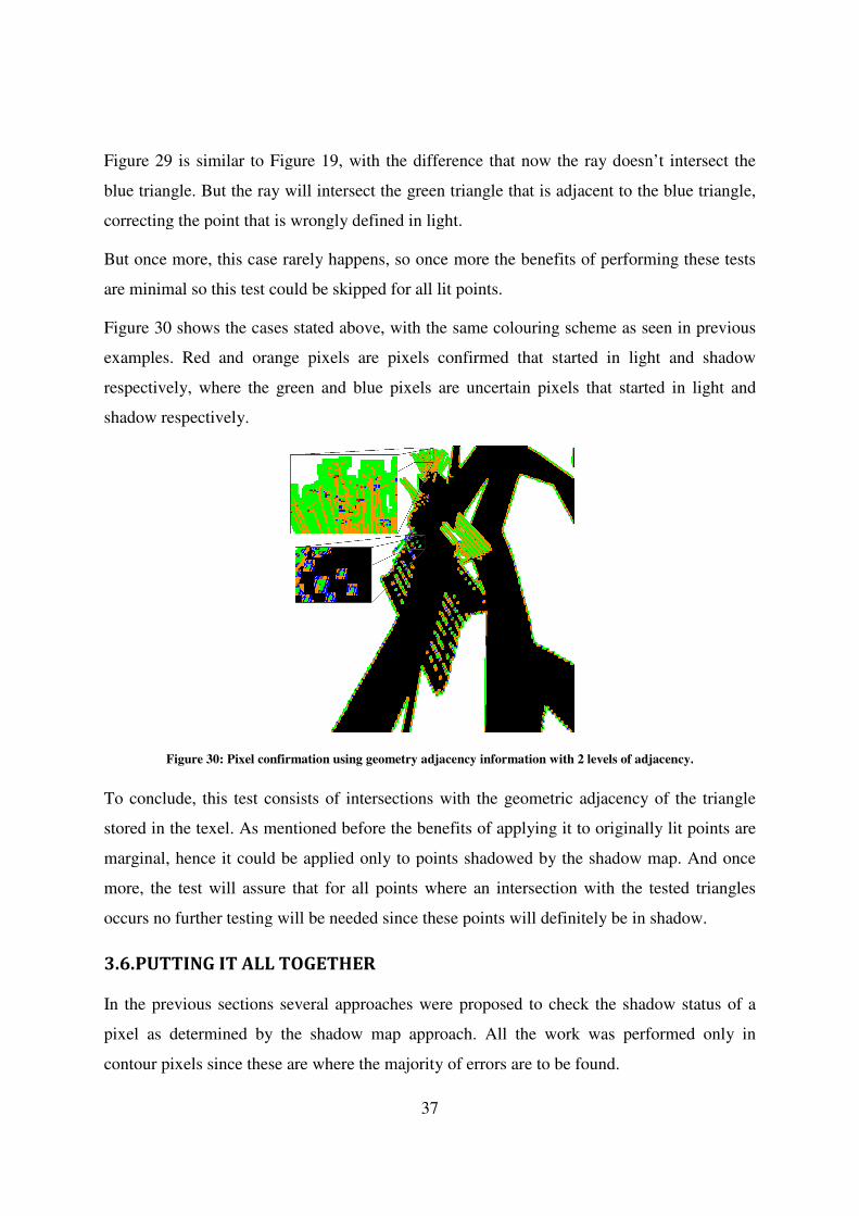
Figure 29 is similar to Figure
blue triangle. But the ray will intersect the green triangle that
correcting the point that is wrongly defined in light.
But once more, this case rarely
are minimal so this test could
Figure 30 shows the cases stated above, with the same colouring scheme as seen in previous
examples. Red and orange pixels are pixels confirmed that started in light a
respectively, where the green and blue pixels are uncertain pixels that started in light and
shadow respectively.
Figure 30: Pixel confirmation using geometry adjacency information with 2 levels of adjacency.
To conclude, this test consists of intersections with the
stored in the texel. As mentioned before the benefits of applying it to originally lit points are
marginal, hence it could be applied only to points shadowed by the shadow
more, the test will assure that
occurs no further testing will be needed
3.6. PUTTING IT ALL TOGETHER
In the previous sections several
pixel as determined by the shadow map approach. All the work was performed only in
contour pixels since these are where the majority of errors are to be found.
37
Figure 19, with the difference that now the ray doesn’t intersect the
blue triangle. But the ray will intersect the green triangle that is adjacent to the blue triangle,
correcting the point that is wrongly defined in light.
But once more, this case rarely happens, so once more the benefits of performing these tests
be skipped for all lit points.
shows the cases stated above, with the same colouring scheme as seen in previous
Red and orange pixels are pixels confirmed that started in light a
respectively, where the green and blue pixels are uncertain pixels that started in light and
: Pixel confirmation using geometry adjacency information with 2 levels of adjacency.
e, this test consists of intersections with the geometric adjacency of the triangle
As mentioned before the benefits of applying it to originally lit points are
marginal, hence it could be applied only to points shadowed by the shadow
more, the test will assure that for all points where an intersection with the tested triangles
further testing will be needed since these points will definitely be in shadow.
OGETHER
In the previous sections several approaches were proposed to check the shadow status of a
pixel as determined by the shadow map approach. All the work was performed only in
contour pixels since these are where the majority of errors are to be found.
, with the difference that now the ray doesn’t intersect the
is adjacent to the blue triangle,
o once more the benefits of performing these tests
shows the cases stated above, with the same colouring scheme as seen in previous
Red and orange pixels are pixels confirmed that started in light and shadow
respectively, where the green and blue pixels are uncertain pixels that started in light and
: Pixel confirmation using geometry adjacency information with 2 levels of adjacency.
adjacency of the triangle
As mentioned before the benefits of applying it to originally lit points are
marginal, hence it could be applied only to points shadowed by the shadow map. And once
all points where an intersection with the tested triangles
since these points will definitely be in shadow.
approaches were proposed to check the shadow status of a
pixel as determined by the shadow map approach. All the work was performed only in
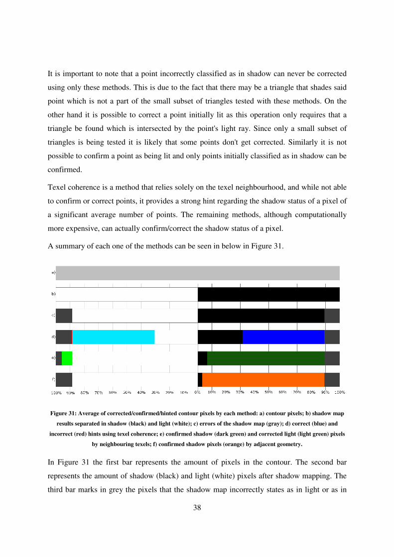
38
It is important to note that a point incorrectly classified as in shadow can never be corrected
using only these methods. This is due to the fact that there may be a triangle that shades said
point which is not a part of the small subset of triangles tested with these methods. On the
other hand it is possible to correct a point initially lit as this operation only requires that a
triangle be found which is intersected by the point's light ray. Since only a small subset of
triangles is being tested it is likely that some points don't get corrected. Similarly it is not
possible to confirm a point as being lit and only points initially classified as in shadow can be
confirmed.
Texel coherence is a method that relies solely on the texel neighbourhood, and while not able
to confirm or correct points, it provides a strong hint regarding the shadow status of a pixel of
a significant average number of points. The remaining methods, although computationally
more expensive, can actually confirm/correct the shadow status of a pixel.
A summary of each one of the methods can be seen in below in Figure 31.
Figure 31: Average of corrected/confirmed/hinted contour pixels by each method: a) contour pixels; b) shadow map
results separated in shadow (black) and light (white); c) errors of the shadow map (gray); d) correct (blue) and
incorrect (red) hints using texel coherence; e) confirmed shadow (dark green) and corrected light (light green) pixels
by neighbouring texels; f) confirmed shadow pixels (orange) by adjacent geometry.
In Figure 31 the first bar represents the amount of pixels in the contour. The second bar
represents the amount of shadow (black) and light (white) pixels after shadow mapping. The
third bar marks in grey the pixels that the shadow map incorrectly states as in light or as in
39
shadow. The fourth bar represents the hinted pixels by the texel coherence method, where the
blue light and dark blue colours represent the correctly hinted pixels and the red colour
represents the incorrectly hinted pixels. The fifth bar represents the results of the
neighbouring texel method, where the dark green represents confirmed shadow pixels and the
light green represents corrected light pixels. Finally, the sixth bar represents the results of the
adjacent geometry method, where the orange colour represents the confirmed shadow pixels.
The colour code found above will be used in similar graphics from here on forth.
From all the methods above, only the neighbouring texels method is actually capable of
correcting the shadow status of a point. Hence this method could in principle be applied as a
standalone method. Although only points initially classified as in light can be corrected the
range of improvement can go all the way up 97.94%. However the improvements are not
perceptually significant as the incorrectly classified pixels in shadow are too prominent.
Another option is to consider these methods as a step whose goal is to reduce the workload of
a regular ray-tracer. In this context, all confirmed/hinted/corrected points would not require
further work, hence reducing the burden of the ray-tracer to verify only the remaining points.
In this section some ways of chaining the previous methods together to improve the shadow
map result and to reduce the workload of a full ray-tracer to obtain the correct shadows will
be proposed.
Texel coherence, as mentioned before, does not correct the shadow status of a pixel, yet it
provides a strong hint of its status. It could be used as the first step, to significantly reduce the
workload of the remaining steps. In a progressive approach, this method could be used in the
first step when the camera is moving to speed things up, and afterwards, when the camera is
still, it could be discarded. Another scenario is for this method to kick in when the frame rate
drops below a defined threshold.
Texel coherence hints from 2.37% to 90.15% of the points initially classified as in shadow,
and 2.42% to 91.70% for those initially classified as lit.
As for the remaining methods these should be applied starting from the least computationally
expensive, the texel neighbourhood, followed by the adjacent triangles method. These
methods will only be applied on points that have not been resolved in the previous steps.
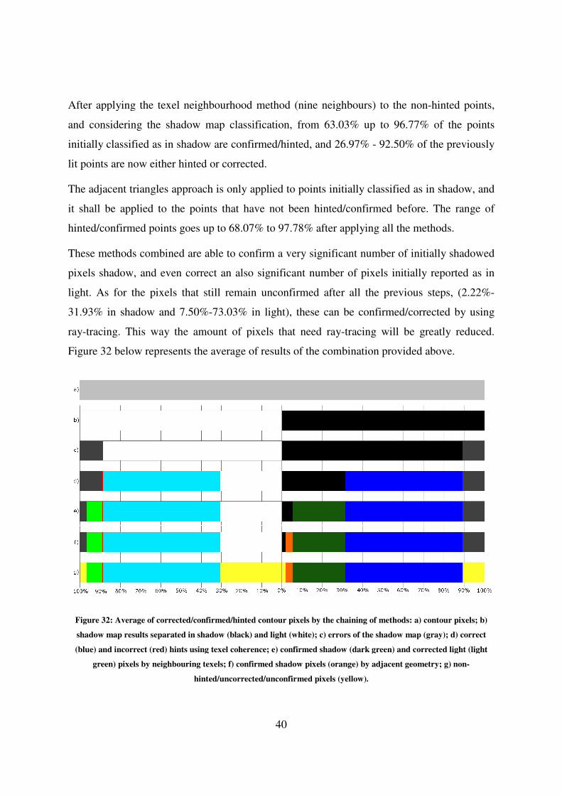
After applying the texel neighbourhood method (nine neighbours) to the non
and considering the shadow map classification, from 63.03% up to 96.77% of the points
initially classified as in shadow are confirmed/hinted, and
lit points are now either hinted or corrected.
The adjacent triangles approach is only applied to points initially classified as in shadow, and
it shall be applied to the points that have not been hinted/confirmed before. The range of
hinted/confirmed points goes up to 68.07% to 97.78% after applying all the methods.
These methods combined are able to confirm a very significant number of initially shadowed
pixels shadow, and even correct an also significant number of pixels initially reporte
light. As for the pixels that still remain unconfirmed after all the previous steps, (2.22%
31.93% in shadow and 7.50%
ray-tracing. This way the amount of pixels that need ray
Figure 32 below represents the average of results of the combination provided above.
Figure 32: Average of corrected/confirmed/hinted contour pixels by
shadow map results separated in shadow (black) and light (white); c) errors of the shadow map (gray); d) correct
(blue) and incorrect (red) hints using
green) pixels by neighbouring texels; f) confirmed shadow pixels (ora
hinted/uncorrected/unconfirmed pixels (yellow).
40
After applying the texel neighbourhood method (nine neighbours) to the non
and considering the shadow map classification, from 63.03% up to 96.77% of the points
hadow are confirmed/hinted, and 26.97% - 92.50% of
lit points are now either hinted or corrected.
The adjacent triangles approach is only applied to points initially classified as in shadow, and
it shall be applied to the points that have not been hinted/confirmed before. The range of
d/confirmed points goes up to 68.07% to 97.78% after applying all the methods.
These methods combined are able to confirm a very significant number of initially shadowed
pixels shadow, and even correct an also significant number of pixels initially reporte
light. As for the pixels that still remain unconfirmed after all the previous steps, (2.22%
31.93% in shadow and 7.50%-73.03% in light), these can be confirmed/corrected by using
tracing. This way the amount of pixels that need ray-tracing will be greatly reduced.
below represents the average of results of the combination provided above.
: Average of corrected/confirmed/hinted contour pixels by the chaining of methods
shadow map results separated in shadow (black) and light (white); c) errors of the shadow map (gray); d) correct
(blue) and incorrect (red) hints using texel coherence; e) confirmed shadow (dark green) and corrected light (light
green) pixels by neighbouring texels; f) confirmed shadow pixels (orange) by adjacent geometry; g) non
hinted/uncorrected/unconfirmed pixels (yellow).
After applying the texel neighbourhood method (nine neighbours) to the non-hinted points,
and considering the shadow map classification, from 63.03% up to 96.77% of the points
92.50% of the previously
The adjacent triangles approach is only applied to points initially classified as in shadow, and
it shall be applied to the points that have not been hinted/confirmed before. The range of
d/confirmed points goes up to 68.07% to 97.78% after applying all the methods.
These methods combined are able to confirm a very significant number of initially shadowed
pixels shadow, and even correct an also significant number of pixels initially reported as in
light. As for the pixels that still remain unconfirmed after all the previous steps, (2.22%-
73.03% in light), these can be confirmed/corrected by using
be greatly reduced.
below represents the average of results of the combination provided above.
s: a) contour pixels; b)
shadow map results separated in shadow (black) and light (white); c) errors of the shadow map (gray); d) correct
texel coherence; e) confirmed shadow (dark green) and corrected light (light
nge) by adjacent geometry; g) non-
41
In Figure 32 the first four bars represent the same as in Figure 31. The remaining bars show
further steps in the chaining of methods. The fifth bar represents the results after the
neighbouring texels method and the sixth bar represents the results after using the adjacent
geometry method. The final bar marks in yellow all pixels that remained non-hinted,
unconfirmed or uncorrected.
3.7. CONCLUSION
This chapter presented a study on the location and identification of shadow mapping errors.
The first goal was to narrow down the location of errors. Shadow map errors can be present
in any part of the image, yet the vast majority seems to be located in average on the contours
of the shadows. Focusing on this area reduces significantly the search for shadow mapping
errors.
The next step was to figure out if it is possible to evaluate the correctness of the shadow
mapping shadow or light status. Several methods were proposed that can confirm the
correctness of a pixel in the rendered scene for pixels in shadow and some of these methods
are even able to determine if a pixel is incorrectly lit.
These methods use information readily available on the shadow map. The adjacency method
also requires a table of adjacencies for each triangle. Adjacencies can be vertex or edge
based.
One of the methods, texel coherence, is not able to either correct/confirm any pixel, yet it
provides a strong hint about its correctness. Few errors are to be found in these hints, and the
method is extremely fast, in fact as fast as PCF shadow mapping.
Since each method has its strengths and weaknesses, an algorithm was proposed to chain
these methods together. The algorithm starts by identifying the contours of the shadow areas
and then proceeds to use each of the methods described in this section. Each method
corrects/confirms a set of pixels, and the remaining uncorrected/unconfirmed pixels pass on
to the next stage.
The methods are only able to confirm that a pixel in shadow is actually in shadow, i.e. they
are unable to determine if a pixel in shadow should be lit. The test is performed with a limited
number of triangles hence there is no guarantee that there is not a triangle in the full data set

42
that covers it. Similarly, for pixels that remain uncorrected in light, these were only tested
with a limited number of triangles, so the same reasoning applies.
At the end of the chain, the percentage of uncorrected/unconfirmed pixels is severely
reduced. These pixels can be correctly shadowed/lit but the information available on does not
allow its verification. To determine the shadow status of these remaining pixels a full ray-
tracer is required. However, applying a full ray-tracer to only these pixels severely reduces
this last step, making it affordable for real-time shadows.
43
4. ALGORITHM TESTING
The descriptions of the approaches referred above were put together after an observation of
some test results of these approaches. In this chapter some of these tests will be observed in
greater detail. These tests consisted in using the proposed approaches to obtain the image
viewed by the camera in a scene. Afterwards these images were compared to their ray-tracer
and shadow mapping equivalents in order to ascertain the quality of the results of the
approach.
This chapter will start by presenting the scenes and viewpoints being tested and the ray-traced
shadows of these scenes. Afterwards this chapter will follow the algorithm proposed in the
previous chapter, presenting an average of all of the tests and the best and worst case
scenarios of the tests of each respective approach when used by itself and also for the
proposed algorithm after passing through the specified approach. As for specifics of the tests
there will be three contour thicknesses that will be tested. These contours will be two, four
and six pixels thick and may also be described by referring to dilations, corresponding to the
simple contour and the contours with one and two dilations respectively. Tests will also be
done with shadow map resolutions of 1024x1024 and 2048x2048, a viewport resolution of
1024x1024 and three viewpoints for each one of the four scenes. The view frustum will have
the minimum size needed to contain the objects being seen by the camera, including also all
the geometry that could influence lighting, from each one of the viewpoints. The light used
will be a directional light in all cases. In order to not clutter up this chapter with result tables,
only some of the results will be displayed here. The results that will be displayed are the best
and worst cases for each shadow map resolution for each one of the approaches by itself, the
proposed algorithm, which will be observed throughout each algorithm step, and also the
average of every result. There will also be an average case that will be followed throughout
the chapter, the “with” viewpoint of the “bench” scene (information of scenes and viewpoints
tested will be observed in detail below) when using a two pixel thick contour and a
2048x2048 resolution shadow map. This case was chosen due to its results being close to
those of the average results. Except if stated otherwise, the results presented here will be the
percentage of pixels in relation to the total amount of pixels inside the contour being tested,
be it the actual total amount, when nothing is referred, or the total amount of light or shadow
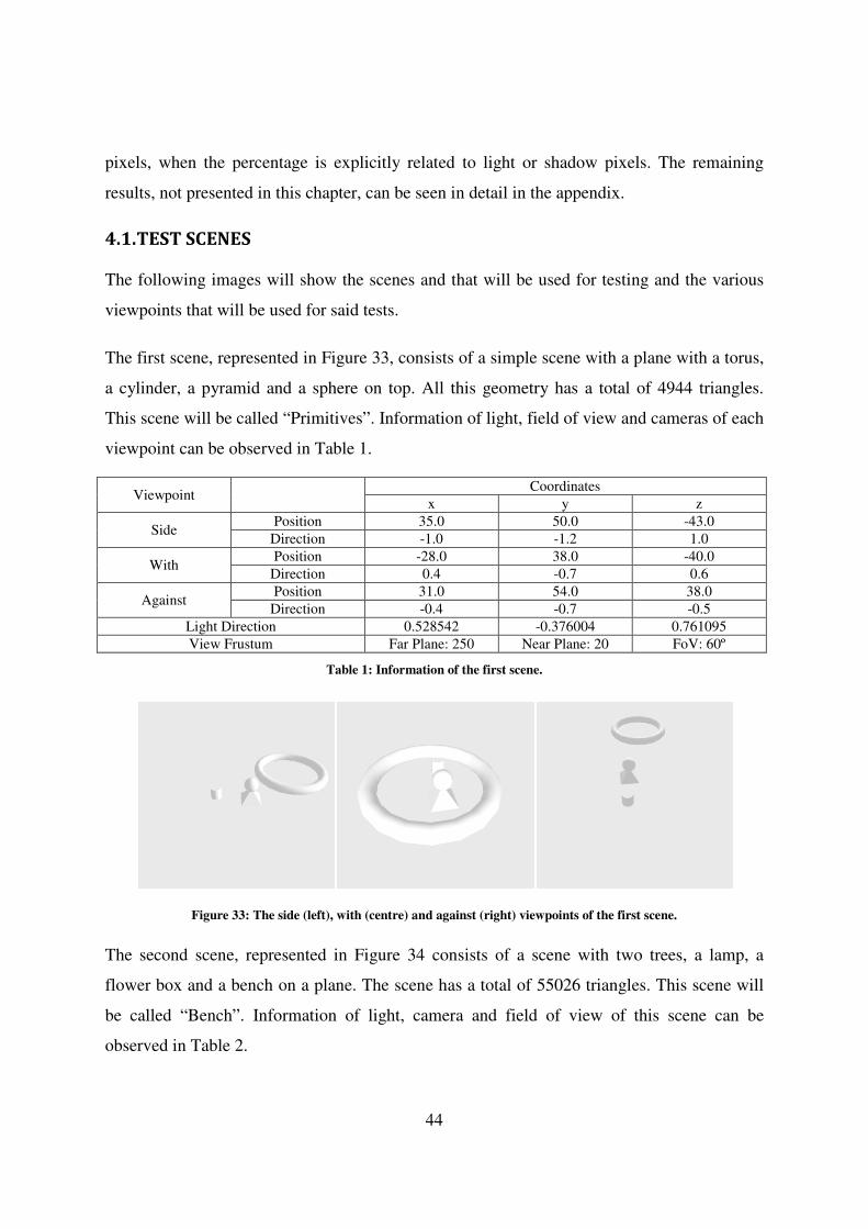
44
pixels, when the percentage is explicitly related to light or shadow pixels. The remaining
results, not presented in this chapter, can be seen in detail in the appendix.
4.1. TEST SCENES
The following images will show the scenes and that will be used for testing and the various
viewpoints that will be used for said tests.
The first scene, represented in Figure 33, consists of a simple scene with a plane with a torus,
a cylinder, a pyramid and a sphere on top. All this geometry has a total of 4944 triangles.
This scene will be called “Primitives”. Information of light, field of view and cameras of each
viewpoint can be observed in Table 1.
Viewpoint Coordinates
x y z
Side Position 35.0 50.0 -43.0
Direction -1.0 -1.2 1.0
With Position -28.0 38.0 -40.0
Direction 0.4 -0.7 0.6
Against Position 31.0 54.0 38.0
Direction -0.4 -0.7 -0.5
Light Direction 0.528542 -0.376004 0.761095
View Frustum Far Plane: 250 Near Plane: 20 FoV: 60º
Table 1: Information of the first scene.
Figure 33: The side (left), with (centre) and against (right) viewpoints of the first scene.
The second scene, represented in Figure 34 consists of a scene with two trees, a lamp, a
flower box and a bench on a plane. The scene has a total of 55026 triangles. This scene will
be called “Bench”. Information of light, camera and field of view of this scene can be
observed in Table 2.
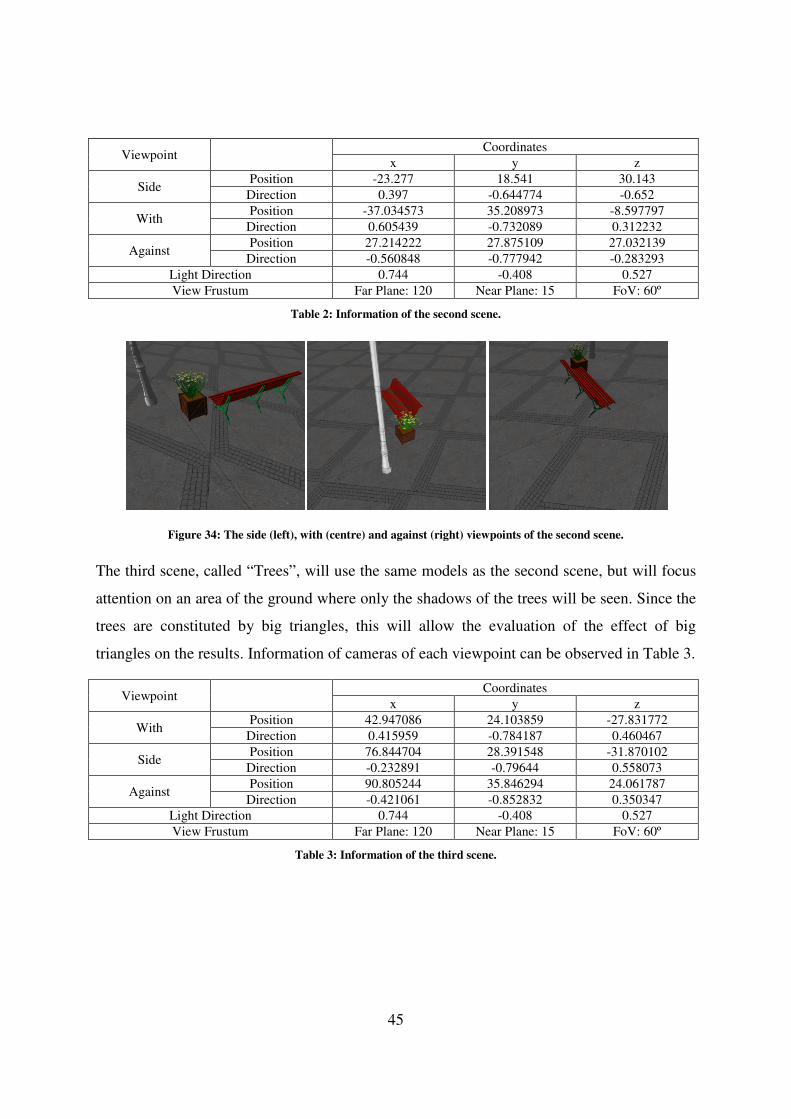
45
Viewpoint Coordinates
x y z
Side Position -23.277 18.541 30.143
Direction 0.397 -0.644774 -0.652
With Position -37.034573 35.208973 -8.597797
Direction 0.605439 -0.732089 0.312232
Against Position 27.214222 27.875109 27.032139
Direction -0.560848 -0.777942 -0.283293
Light Direction 0.744 -0.408 0.527
View Frustum Far Plane: 120 Near Plane: 15 FoV: 60º
Table 2: Information of the second scene.
Figure 34: The side (left), with (centre) and against (right) viewpoints of the second scene.
The third scene, called “Trees”, will use the same models as the second scene, but will focus
attention on an area of the ground where only the shadows of the trees will be seen. Since the
trees are constituted by big triangles, this will allow the evaluation of the effect of big
triangles on the results. Information of cameras of each viewpoint can be observed in Table 3.
Viewpoint Coordinates
x y z
With Position 42.947086 24.103859 -27.831772
Direction 0.415959 -0.784187 0.460467
Side Position 76.844704 28.391548 -31.870102
Direction -0.232891 -0.79644 0.558073
Against Position 90.805244 35.846294 24.061787
Direction -0.421061 -0.852832 0.350347
Light Direction 0.744 -0.408 0.527
View Frustum Far Plane: 120 Near Plane: 15 FoV: 60º
Table 3: Information of the third scene.
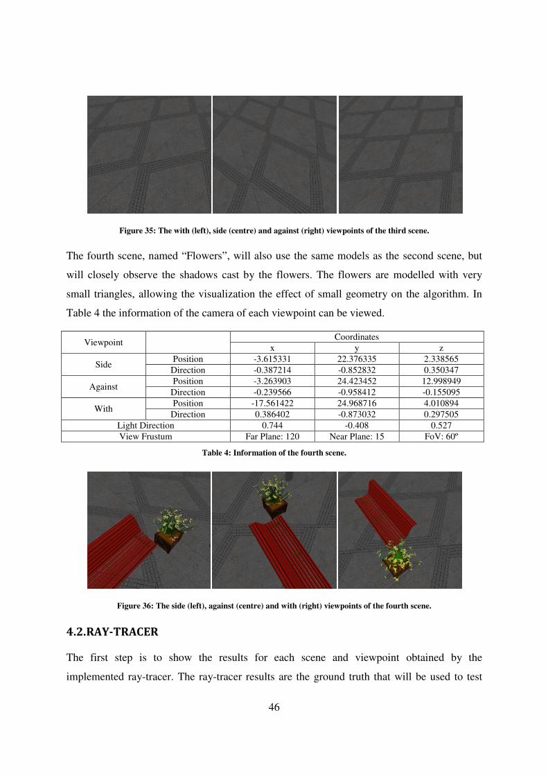
46
Figure 35: The with (left), side (centre) and against (right) viewpoints of the third scene.
The fourth scene, named “Flowers”, will also use the same models as the second scene, but
will closely observe the shadows cast by the flowers. The flowers are modelled with very
small triangles, allowing the visualization the effect of small geometry on the algorithm. In
Table 4 the information of the camera of each viewpoint can be viewed.
Viewpoint Coordinates
x y z
Side Position -3.615331 22.376335 2.338565
Direction -0.387214 -0.852832 0.350347
Against Position -3.263903 24.423452 12.998949
Direction -0.239566 -0.958412 -0.155095
With Position -17.561422 24.968716 4.010894
Direction 0.386402 -0.873032 0.297505
Light Direction 0.744 -0.408 0.527
View Frustum Far Plane: 120 Near Plane: 15 FoV: 60º
Table 4: Information of the fourth scene.
Figure 36: The side (left), against (centre) and with (right) viewpoints of the fourth scene.
4.2. RAY-TRACER
The first step is to show the results for each scene and viewpoint obtained by the
implemented ray-tracer. The ray-tracer results are the ground truth that will be used to test
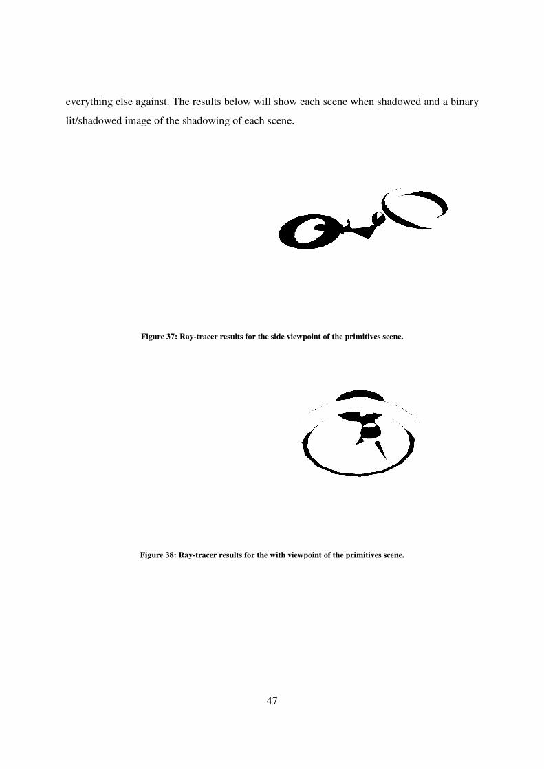
everything else against. The results below will show each scene when shadowed and a binary
lit/shadowed image of the shadowing of each scene.
Figure 37: Ray-tracer results for
Figure 38: Ray-tracer results for the with viewpoint of the primitives scene.
47
The results below will show each scene when shadowed and a binary
lit/shadowed image of the shadowing of each scene.
tracer results for the side viewpoint of the primitives scene.
tracer results for the with viewpoint of the primitives scene.
The results below will show each scene when shadowed and a binary
the side viewpoint of the primitives scene.
tracer results for the with viewpoint of the primitives scene.
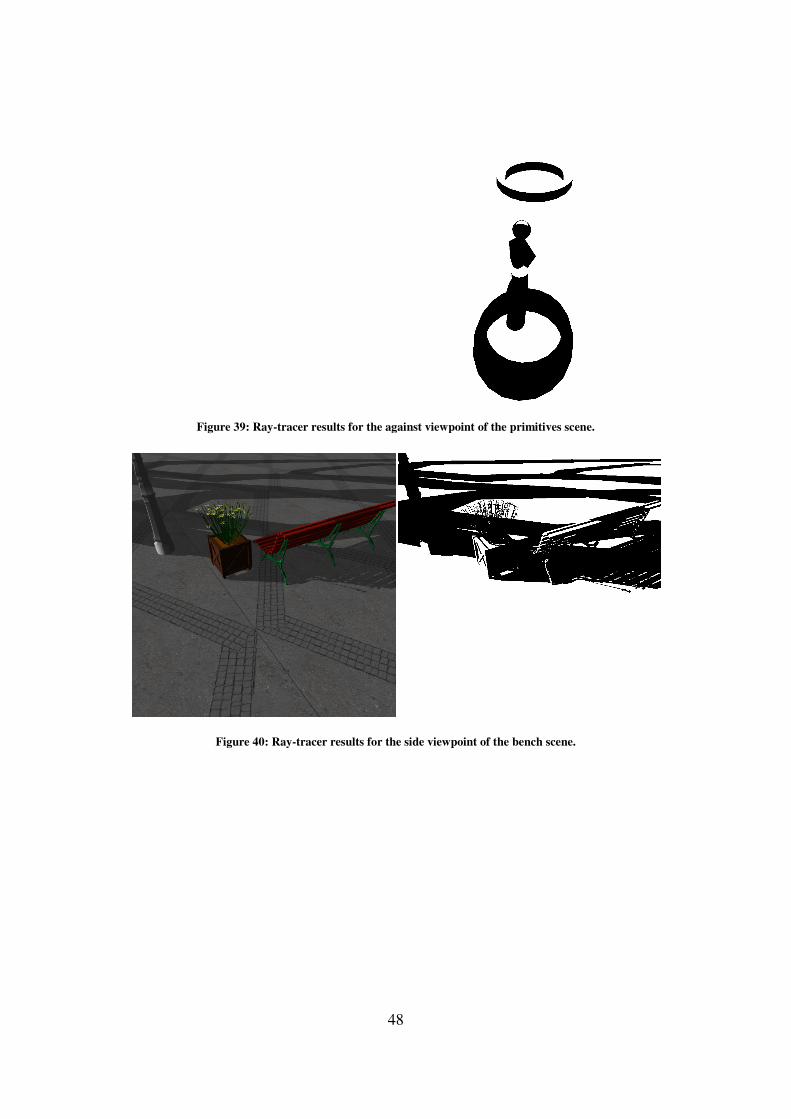
Figure 39: Ray-tracer results for the against viewpoint of the primitives scen
Figure 40: Ray
48
tracer results for the against viewpoint of the primitives scen
: Ray-tracer results for the side viewpoint of the bench scene.
tracer results for the against viewpoint of the primitives scene.
tracer results for the side viewpoint of the bench scene.
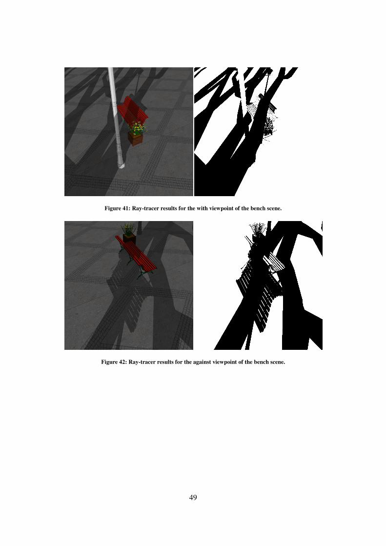
Figure 41: Ray
Figure 42: Ray-
49
: Ray-tracer results for the with viewpoint of the bench scene.
-tracer results for the against viewpoint of the bench scene.
tracer results for the with viewpoint of the bench scene.
esults for the against viewpoint of the bench scene.
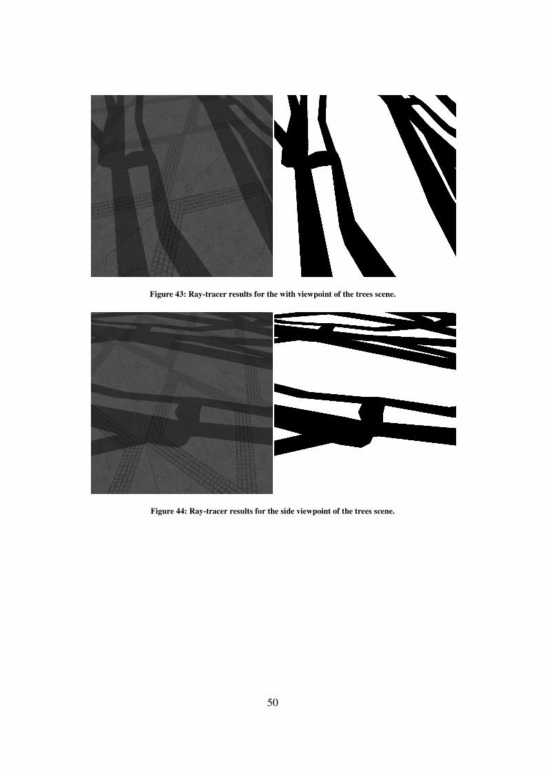
Figure 43: Ray
Figure 44: Ray
50
: Ray-tracer results for the with viewpoint of the trees scene.
: Ray-tracer results for the side viewpoint of the trees scene.
tracer results for the with viewpoint of the trees scene.
tracer results for the side viewpoint of the trees scene.
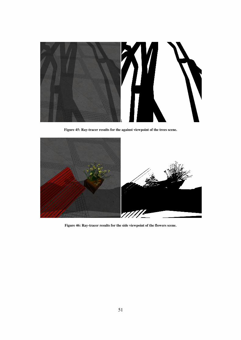
Figure 45: Ray
Figure 46: Ray
51
: Ray-tracer results for the against viewpoint of the trees scene.
: Ray-tracer results for the side viewpoint of the flowers scene.
tracer results for the against viewpoint of the trees scene.
tracer results for the side viewpoint of the flowers scene.
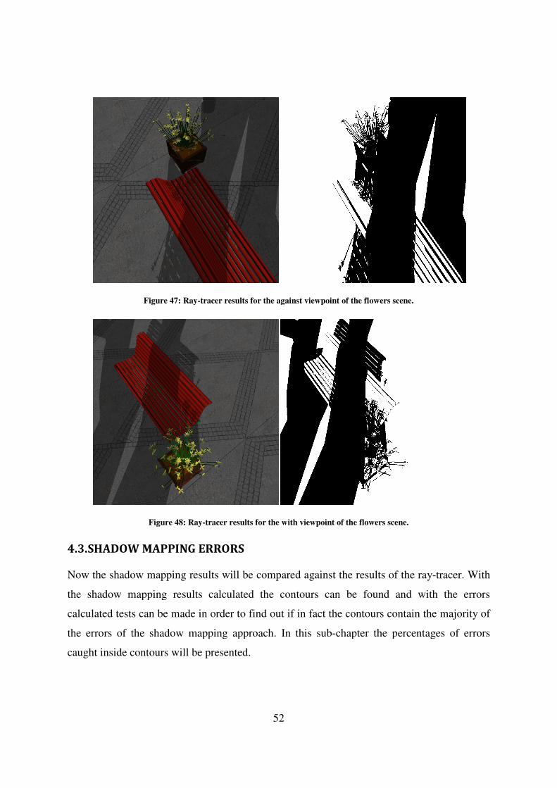
Figure 47: Ray-tracer
Figure 48: Ray
4.3. SHADOW MAPPING E
Now the shadow mapping results will be
the shadow mapping results calculated the contours can be found
calculated tests can be made in order to find out if in fact the contours contain the majority of
the errors of the shadow mapping approach.
caught inside contours will be presented.
52
tracer results for the against viewpoint of the flowers scene.
: Ray-tracer results for the with viewpoint of the flowers scene.
ERRORS
pping results will be compared against the results of the
the shadow mapping results calculated the contours can be found and with the errors
tests can be made in order to find out if in fact the contours contain the majority of
the errors of the shadow mapping approach. In this sub-chapter the percentages of errors
caught inside contours will be presented.
results for the against viewpoint of the flowers scene.
tracer results for the with viewpoint of the flowers scene.
against the results of the ray-tracer. With
and with the errors
tests can be made in order to find out if in fact the contours contain the majority of
apter the percentages of errors

Average
Scene --
Viewpoint --
Contour Size --
Caught Errors (%) 92.41
Table
As seen in Table 5, in average over 90% of the shadow map errors are caught inside the
contours. Below are the images of the results of the best
The contours are marked with green, the errors outside the contour are in blue and the errors
inside the contour are in red and yellow if the pixel is incorrectly in light and shadow
respectively.
Figure 49: Best case of shadow
In the best case scenarios seen in
small amount of errors, so by using a 6 pixel thick contour, this small amount of errors will
be caught inside the contours.
53
Shadow Map
1024x1024 2048x2048
Best Case Worst Case Best Case Worst Case
Primitives Primitives Primitives Flowers
Side/With Against Side Side
6 pixels 2 pixels 6 pixels 2 pixels
100.00 57.42 100.00 81.00
Table 5: Percentages of errors inside the contours.
, in average over 90% of the shadow map errors are caught inside the
Below are the images of the results of the best, worst and medium
The contours are marked with green, the errors outside the contour are in blue and the errors
inside the contour are in red and yellow if the pixel is incorrectly in light and shadow
: Best case of shadow map errors being caught inside contours with a 2048x2048 shadow map
seen in above, with both shadow map resolutions the results
y using a 6 pixel thick contour, this small amount of errors will
Average
Case
Worst Case
Flowers Bench
Side With
2 pixels 2 pixels
81.00 97.12
, in average over 90% of the shadow map errors are caught inside the
and medium case scenarios.
The contours are marked with green, the errors outside the contour are in blue and the errors
inside the contour are in red and yellow if the pixel is incorrectly in light and shadow
with a 2048x2048 shadow map.
ith both shadow map resolutions the results have a
y using a 6 pixel thick contour, this small amount of errors will
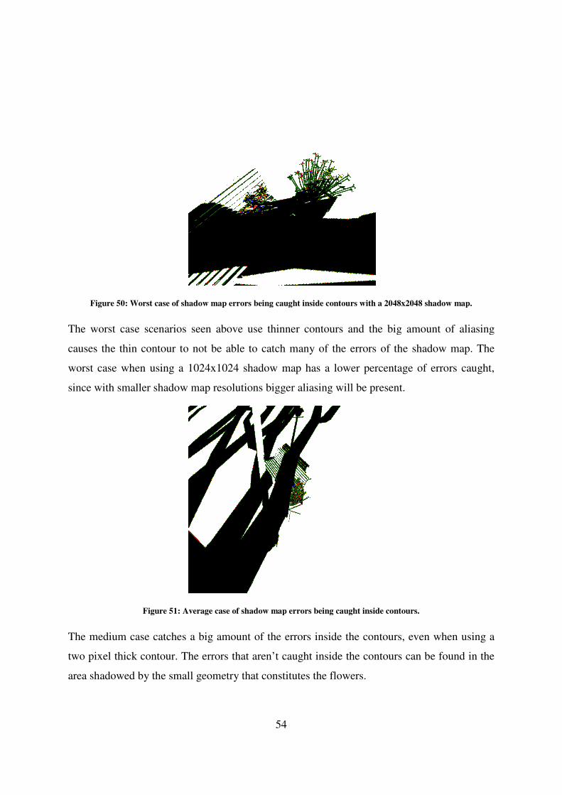
Figure 50: Worst case of shadow map errors being caught inside contours with a 2048x2048 shadow map.
The worst case scenarios seen
causes the thin contour to not be able to catch many of the errors of the shadow map.
worst case when using a 1024x1024 shadow map has a lower percentage of errors caught,
since with smaller shadow map resolutions bigger aliasing will be present.
Figure 51: Average
The medium case catches a big amount of the errors inside the contours, even when using a
two pixel thick contour. The errors that aren’t caught inside the contour
area shadowed by the small geometry that constitutes the flowers.
54
: Worst case of shadow map errors being caught inside contours with a 2048x2048 shadow map.
seen above use thinner contours and the big amount of aliasing
he thin contour to not be able to catch many of the errors of the shadow map.
worst case when using a 1024x1024 shadow map has a lower percentage of errors caught,
since with smaller shadow map resolutions bigger aliasing will be present.
Average case of shadow map errors being caught inside contours.
The medium case catches a big amount of the errors inside the contours, even when using a
two pixel thick contour. The errors that aren’t caught inside the contours can be found in the
area shadowed by the small geometry that constitutes the flowers.
: Worst case of shadow map errors being caught inside contours with a 2048x2048 shadow map.
he big amount of aliasing
he thin contour to not be able to catch many of the errors of the shadow map. The
worst case when using a 1024x1024 shadow map has a lower percentage of errors caught,
case of shadow map errors being caught inside contours.
The medium case catches a big amount of the errors inside the contours, even when using a
s can be found in the

55
Also, to be used as comparison with the proposed approaches, the information of the
percentage of incorrect pixels of the contour is presented below.
Average
Shadow Map Average
Case 1024x1024 2048x2048
Best Case Worst Case Best Case Worst Case
Scene -- Primitives Trees Primitives Trees Bench
Viewpoint -- With Against With With With
Contour Size -- 6 pixels 2 pixels 6 pixels 2 pixels 2 pixels
Errors (%) 11.09 3.40 26.68 1.75 20.50 5.06
Errors in Light (%) 11.50 3.06 25.41 1.41 18.93 4.31
Errors in Shadow
(%) 10.71 3.89 27.93 2.22 22.07 5.99
Table 6: Percentage of contour pixels that are incorrect.
Figure 52 below presents the average of results for the shadow map separated by contour
thickness. Each bar is divided in three smaller bars corresponding, from top to bottom, to the
2, 4 and 6 pixel thick contours.
Figure 52: Average shadow map results separated by contour thickness with a 1024x1024 shadow map (top) and a
2048x2048 shadow map (bottom).
4.4. USING TEXEL COHERENCE
Now the results of the texel coherence will be presented. Since this is the first step in the
proposed algorithm, the results of using this approach by itself and within the algorithm are
the same.
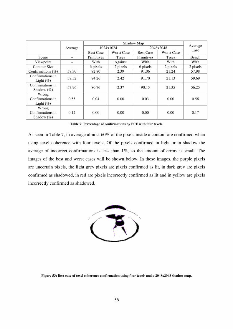
Average
Scene --
Viewpoint --
Contour Size --
Confirmations (%) 58.30
Confirmations in
Light (%) 58.52
Confirmations in
Shadow (%) 57.96
Wrong
Confirmations in
Light (%)
0.55
Wrong
Confirmations in
Shadow (%)
0.12
Table 7: Percentage of confirmations by PCF with four texels.
As seen in Table 7, in average almost 60% of the pixels inside a contour are confirmed when
using texel coherence with four texels. Of the pixels confirmed in light or in shadow the
average of incorrect confirmations is less than 1%, so the amount of errors is small. The
images of the best and worst cases will be shown below.
are uncertain pixels, the light grey pixels are pixels confirmed as lit, in dark grey are pixels
confirmed as shadowed, in red are pixels incorrectly confirmed as
incorrectly confirmed as shadowed.
Figure 53: Best case of texel coherence confirmation using four texels
56
Shadow Map
1024x1024 2048x2048
Best Case Worst Case Best Case Worst Case
Primitives Trees Primitives Trees
With Against With With
6 pixels 2 pixels 6 pixels 2 pixels
82.80 2.39 91.06 21.24
84.26 2.42 91.70 21.13
80.76 2.37 90.15 21.35
0.04 0.00 0.03 0.00
0.00 0.00 0.00 0.00
: Percentage of confirmations by PCF with four texels.
, in average almost 60% of the pixels inside a contour are confirmed when
using texel coherence with four texels. Of the pixels confirmed in light or in shadow the
ations is less than 1%, so the amount of errors is small. The
images of the best and worst cases will be shown below. In these images, the purple pixels
are uncertain pixels, the light grey pixels are pixels confirmed as lit, in dark grey are pixels
med as shadowed, in red are pixels incorrectly confirmed as lit and in yellow are pixels
incorrectly confirmed as shadowed.
: Best case of texel coherence confirmation using four texels and a 2048x2048 shadow map
Average
Case
Worst Case
Trees Bench
With With
2 pixels 2 pixels
21.24 57.98
21.13 59.69
21.35 56.25
0.00 0.56
0.00 0.17
, in average almost 60% of the pixels inside a contour are confirmed when
using texel coherence with four texels. Of the pixels confirmed in light or in shadow the
ations is less than 1%, so the amount of errors is small. The
In these images, the purple pixels
are uncertain pixels, the light grey pixels are pixels confirmed as lit, in dark grey are pixels
lit and in yellow are pixels
and a 2048x2048 shadow map.
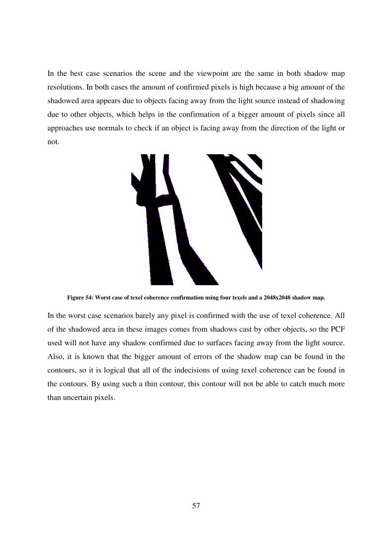
In the best case scenarios the scene and the viewpoint are the same in both shadow map
resolutions. In both cases the amount of confirmed pixels is high
shadowed area appears due to objects facing away from the light source instead of
due to other objects, which helps in the confirmation of a bigger amount of pixels
approaches use normals to check if an object is facing away from the direction of the light or
not.
Figure 54: Worst case of texel coherence confirmation using four texels and a 2048x2048 shadow map.
In the worst case scenarios barely any pixel is confirmed with the use of texel coherence. All
of the shadowed area in these
used will not have any shadow confirmed due to surfaces facing away from the light source.
Also, it is known that the bigger amount of errors of the shadow map can be found in the
contours, so it is logical that all of the indecisions of using texel co
the contours. By using such a thin contour, this contour will not be able to catch much more
than uncertain pixels.
57
the scene and the viewpoint are the same in both shadow map
the amount of confirmed pixels is high because a big amount of the
shadowed area appears due to objects facing away from the light source instead of
due to other objects, which helps in the confirmation of a bigger amount of pixels
approaches use normals to check if an object is facing away from the direction of the light or
texel coherence confirmation using four texels and a 2048x2048 shadow map.
barely any pixel is confirmed with the use of texel coherence. All
e images comes from shadows cast by other objects, so the
used will not have any shadow confirmed due to surfaces facing away from the light source.
Also, it is known that the bigger amount of errors of the shadow map can be found in the
contours, so it is logical that all of the indecisions of using texel coherence can be found in
the contours. By using such a thin contour, this contour will not be able to catch much more
the scene and the viewpoint are the same in both shadow map
a big amount of the
shadowed area appears due to objects facing away from the light source instead of shadowing
due to other objects, which helps in the confirmation of a bigger amount of pixels since all
approaches use normals to check if an object is facing away from the direction of the light or
texel coherence confirmation using four texels and a 2048x2048 shadow map.
barely any pixel is confirmed with the use of texel coherence. All
comes from shadows cast by other objects, so the PCF
used will not have any shadow confirmed due to surfaces facing away from the light source.
Also, it is known that the bigger amount of errors of the shadow map can be found in the
herence can be found in
the contours. By using such a thin contour, this contour will not be able to catch much more
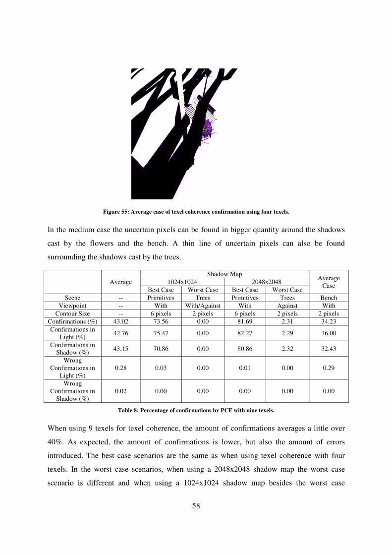
Figure 55: Average
In the medium case the uncertain pixels can be found in bigger quantity around the shadows
cast by the flowers and the bench. A thin line of uncertain pixels can also be found
surrounding the shadows cast by the trees.
Average
Scene --
Viewpoint --
Contour Size --
Confirmations (%) 43.02
Confirmations in
Light (%) 42.76
Confirmations in
Shadow (%) 43.15
Wrong
Confirmations in
Light (%)
0.28
Wrong
Confirmations in
Shadow (%)
0.02
Table 8: Percentage of confirmations by PCF with nine texels.
When using 9 texels for texel coherence, the amount of confirmations averages a little over
40%. As expected, the amount of confirmations is lower, but also th
introduced. The best case scenarios are the same as when using texel coherence with four
texels. In the worst case scenario
scenario is different and when using a 1024x1024 shadow map be
58
Average case of texel coherence confirmation using four texels.
case the uncertain pixels can be found in bigger quantity around the shadows
cast by the flowers and the bench. A thin line of uncertain pixels can also be found
surrounding the shadows cast by the trees.
Shadow Map
1024x1024 2048x2048
Best Case Worst Case Best Case Worst Case
Primitives Trees Primitives Trees
With With/Against With Against
6 pixels 2 pixels 6 pixels 2 pixels
73.56 0.00 81.69 2.31
75.47 0.00 82.27 2.29
70.86 0.00 80.86 2.32
0.03 0.00 0.01 0.00
0.00 0.00 0.00 0.00
: Percentage of confirmations by PCF with nine texels.
When using 9 texels for texel coherence, the amount of confirmations averages a little over
40%. As expected, the amount of confirmations is lower, but also the amount of errors
The best case scenarios are the same as when using texel coherence with four
he worst case scenarios, when using a 2048x2048 shadow map the worst case
scenario is different and when using a 1024x1024 shadow map besides the worst case
case of texel coherence confirmation using four texels.
case the uncertain pixels can be found in bigger quantity around the shadows
cast by the flowers and the bench. A thin line of uncertain pixels can also be found
Average
Case
Worst Case
Trees Bench
Against With
2 pixels 2 pixels
2.31 34.23
2.29 36.00
2.32 32.43
0.00 0.29
0.00 0.00
When using 9 texels for texel coherence, the amount of confirmations averages a little over
e amount of errors
The best case scenarios are the same as when using texel coherence with four
when using a 2048x2048 shadow map the worst case
sides the worst case
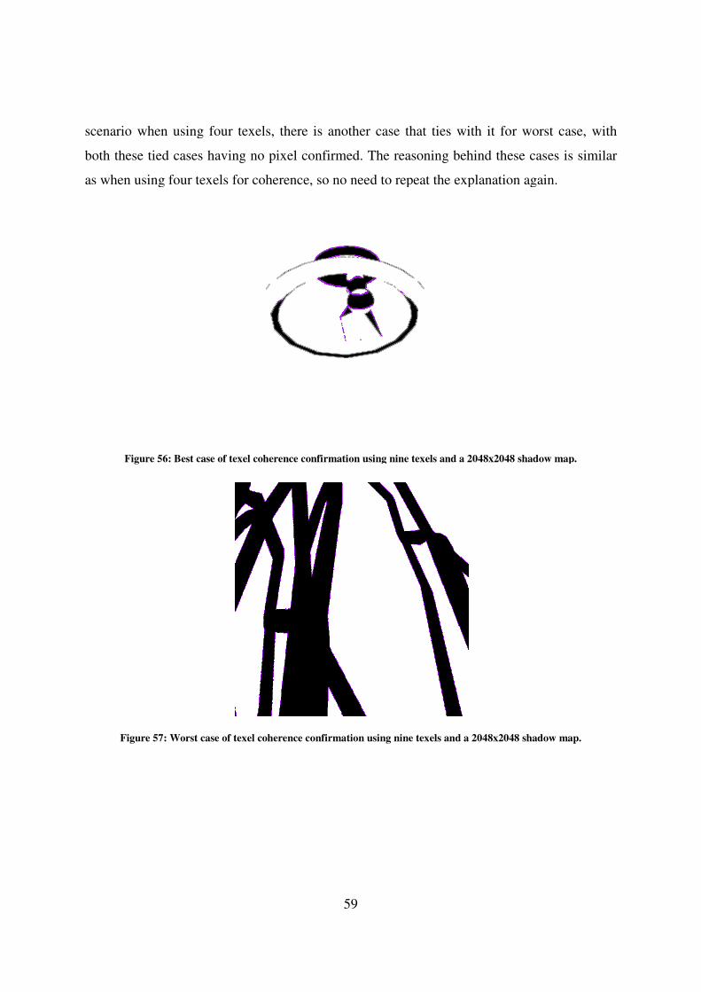
scenario when using four texels, there is another case that ties with it for worst case, with
both these tied cases having no pixel confirmed. The reason
as when using four texels for coherence, so no n
Figure 56: Best case of texel coherence confirmation using nine texels
Figure 57: Worst case of texel coherence confirmation using nine
59
scenario when using four texels, there is another case that ties with it for worst case, with
no pixel confirmed. The reasoning behind these cases
as when using four texels for coherence, so no need to repeat the explanation again.
: Best case of texel coherence confirmation using nine texels and a 2048x2048 shadow map
: Worst case of texel coherence confirmation using nine texels and a 2048x2048 shadow map.
scenario when using four texels, there is another case that ties with it for worst case, with
these cases is similar
eed to repeat the explanation again.
and a 2048x2048 shadow map.
texels and a 2048x2048 shadow map.
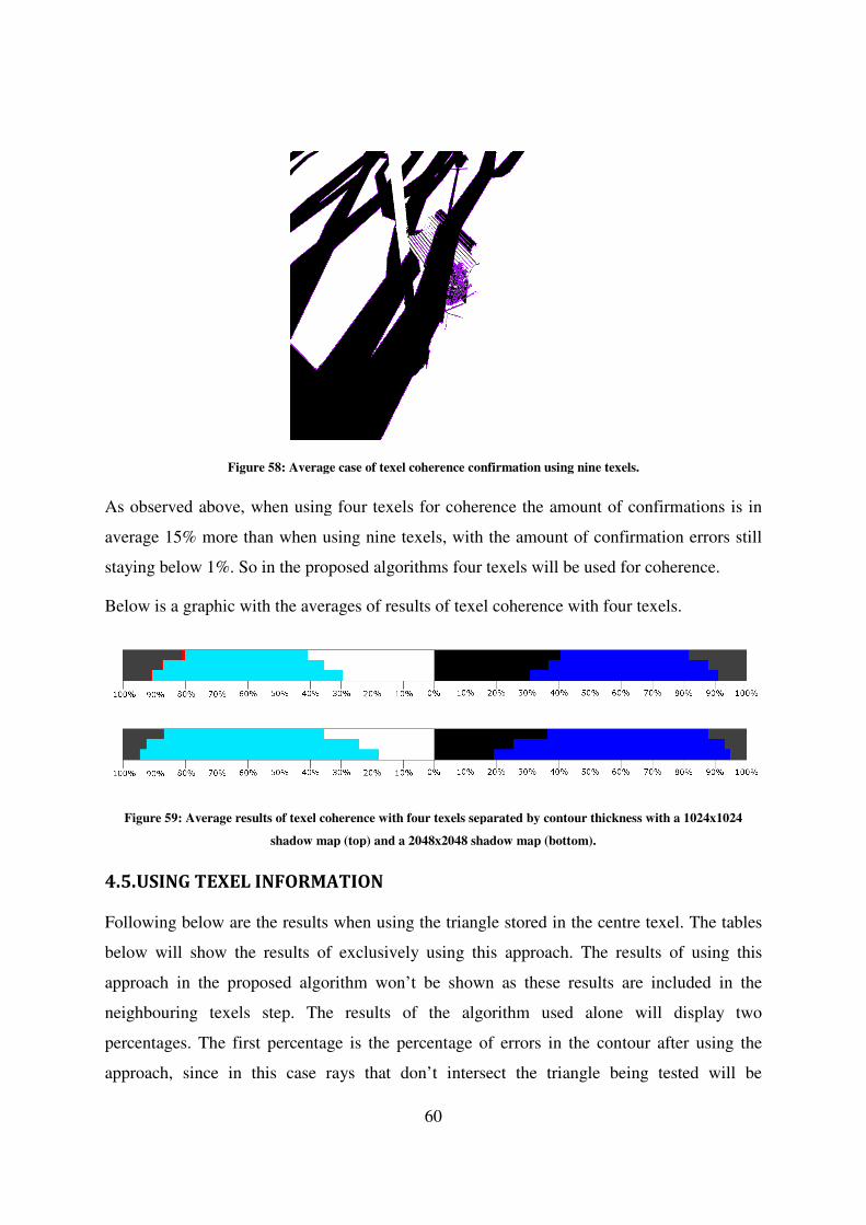
Figure 58: Average
As observed above, when using four texels for coherence the amount of confirmations is in
average 15% more than when us
staying below 1%. So in the proposed algorithms four texels will be used for coherence.
Below is a graphic with the averages of results of texel coherence with four texels.
Figure 59: Average results of texel
shadow map (top) and a 2048x2048 shadow map (bottom).
4.5. USING TEXEL INFORMATION
Following below are the results
below will show the results of
approach in the proposed algorithm
neighbouring texels step. The results of
percentages. The first percentage
approach, since in this case rays that don’t intersect the triangle being tested will be
60
Average case of texel coherence confirmation using nine texels.
As observed above, when using four texels for coherence the amount of confirmations is in
average 15% more than when using nine texels, with the amount of confirmation errors still
staying below 1%. So in the proposed algorithms four texels will be used for coherence.
Below is a graphic with the averages of results of texel coherence with four texels.
results of texel coherence with four texels separated by contour thickness with a 1024x1024
shadow map (top) and a 2048x2048 shadow map (bottom).
NFORMATION
Following below are the results when using the triangle stored in the centre texel
below will show the results of exclusively using this approach. The results of using this
in the proposed algorithm won’t be shown as these results are included in the
The results of the algorithm used alone
percentage is the percentage of errors in the contour after using the
, since in this case rays that don’t intersect the triangle being tested will be
case of texel coherence confirmation using nine texels.
As observed above, when using four texels for coherence the amount of confirmations is in
ing nine texels, with the amount of confirmation errors still
staying below 1%. So in the proposed algorithms four texels will be used for coherence.
Below is a graphic with the averages of results of texel coherence with four texels.
separated by contour thickness with a 1024x1024
stored in the centre texel. The tables
he results of using this
won’t be shown as these results are included in the
will display two
errors in the contour after using the
, since in this case rays that don’t intersect the triangle being tested will be
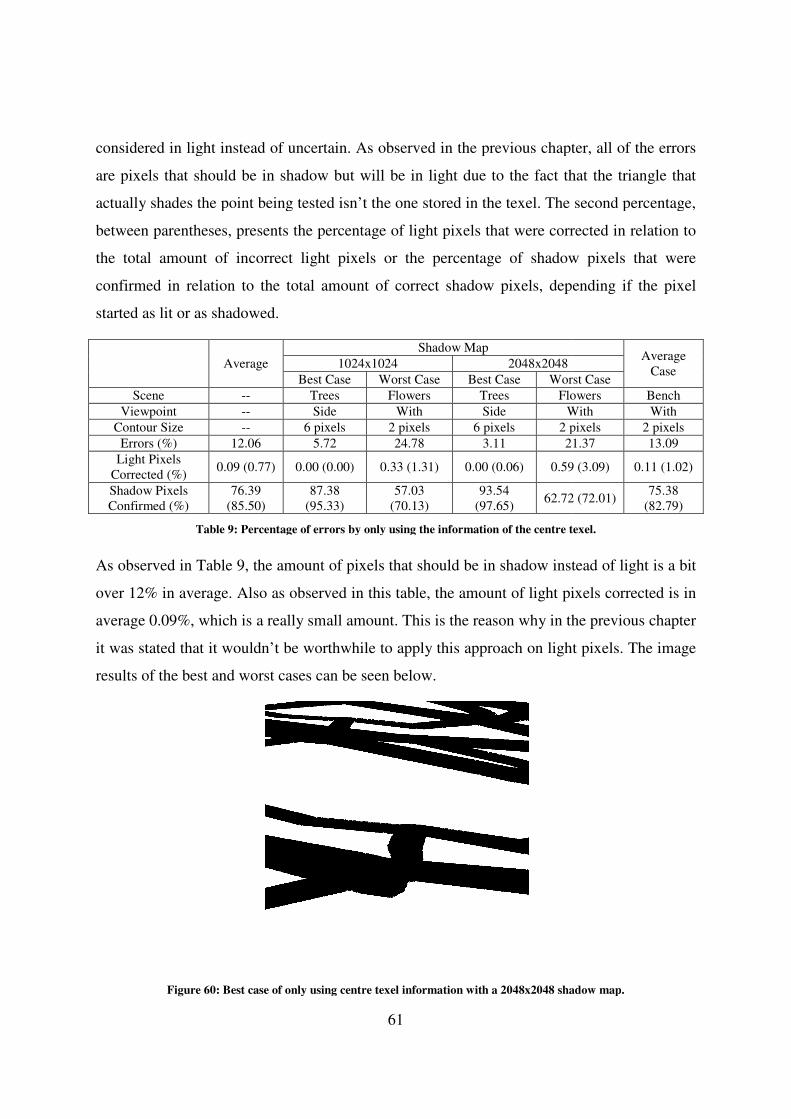
considered in light instead of
are pixels that should be in shadow but will be in light due to the fact that the triangle that
actually shades the point being tested isn’t the one stored in the texel.
between parentheses, presents the percentage of light pixels that were corrected in relation to
the total amount of incorrect light pixels or the percentage of shadow pixels that were
confirmed in relation to the total amount of correct shadow pixels, d
started as lit or as shadowed.
Average
Scene --
Viewpoint --
Contour Size --
Errors (%) 12.06
Light Pixels
Corrected (%) 0.09 (0.77)
Shadow Pixels
Confirmed (%)
76.39
(85.50)
Table 9: Percentage of errors by only using the information of the centre texel.
As observed in Table 9, the amount of pixels that should be in shadow instead of light is a bit
over 12% in average. Also as observed in this table, the amount of light pixels corrected is in
average 0.09%, which is a really small amount. This is the reason why in the previous chapter
it was stated that it wouldn’t be worthwhile to apply this approach on light pixels.
results of the best and worst cases can be seen below.
Figure 60: Best case of only using centre texel information
61
considered in light instead of uncertain. As observed in the previous chapter, all of the errors
are pixels that should be in shadow but will be in light due to the fact that the triangle that
actually shades the point being tested isn’t the one stored in the texel. The second percentag
between parentheses, presents the percentage of light pixels that were corrected in relation to
the total amount of incorrect light pixels or the percentage of shadow pixels that were
confirmed in relation to the total amount of correct shadow pixels, depending if the pixel
Shadow Map
1024x1024 2048x2048
Best Case Worst Case Best Case Worst Case
Trees Flowers Trees Flowers
Side With Side With
6 pixels 2 pixels 6 pixels 2 pixels
5.72 24.78 3.11 21.37
0.00 (0.00) 0.33 (1.31) 0.00 (0.06) 0.59
87.38
(95.33)
57.03
(70.13)
93.54
(97.65) 62.72
: Percentage of errors by only using the information of the centre texel.
, the amount of pixels that should be in shadow instead of light is a bit
Also as observed in this table, the amount of light pixels corrected is in
s a really small amount. This is the reason why in the previous chapter
it was stated that it wouldn’t be worthwhile to apply this approach on light pixels.
results of the best and worst cases can be seen below.
: Best case of only using centre texel information with a 2048x2048 shadow map
. As observed in the previous chapter, all of the errors
are pixels that should be in shadow but will be in light due to the fact that the triangle that
The second percentage,
between parentheses, presents the percentage of light pixels that were corrected in relation to
the total amount of incorrect light pixels or the percentage of shadow pixels that were
epending if the pixel
Average
Case
Worst Case
Flowers Bench
With With
2 pixels 2 pixels
21.37 13.09
0.59 (3.09) 0.11 (1.02)
62.72 (72.01) 75.38
(82.79)
: Percentage of errors by only using the information of the centre texel.
, the amount of pixels that should be in shadow instead of light is a bit
Also as observed in this table, the amount of light pixels corrected is in
s a really small amount. This is the reason why in the previous chapter
it was stated that it wouldn’t be worthwhile to apply this approach on light pixels. The image
with a 2048x2048 shadow map.
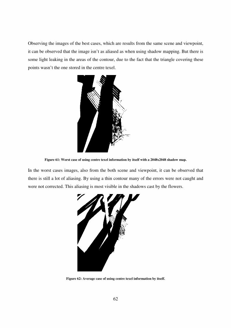
Observing the images of the best case
it can be observed that the image isn’t as aliased as when using shadow mapping.
some light leaking in the areas of the contour, due to the fact that the triangle covering these
points wasn’t the one stored in the centre texel.
Figure 61: Worst case of using centre texel information by itself wit
In the worst cases images, also from the both scene and viewpoint,
there is still a lot of aliasing. By using a thin contour many of the errors were not caught and
were not corrected. This aliasing is most
Figure 62: Average
62
of the best cases, which are results from the same scene and viewpoint,
it can be observed that the image isn’t as aliased as when using shadow mapping.
some light leaking in the areas of the contour, due to the fact that the triangle covering these
points wasn’t the one stored in the centre texel.
: Worst case of using centre texel information by itself with a 2048x2048 shadow map.
s, also from the both scene and viewpoint, it can be observed that
there is still a lot of aliasing. By using a thin contour many of the errors were not caught and
were not corrected. This aliasing is most visible in the shadows cast by the flowers.
Average case of using centre texel information by itself.
s, which are results from the same scene and viewpoint,
it can be observed that the image isn’t as aliased as when using shadow mapping. But there is
some light leaking in the areas of the contour, due to the fact that the triangle covering these
h a 2048x2048 shadow map.
it can be observed that
there is still a lot of aliasing. By using a thin contour many of the errors were not caught and
visible in the shadows cast by the flowers.
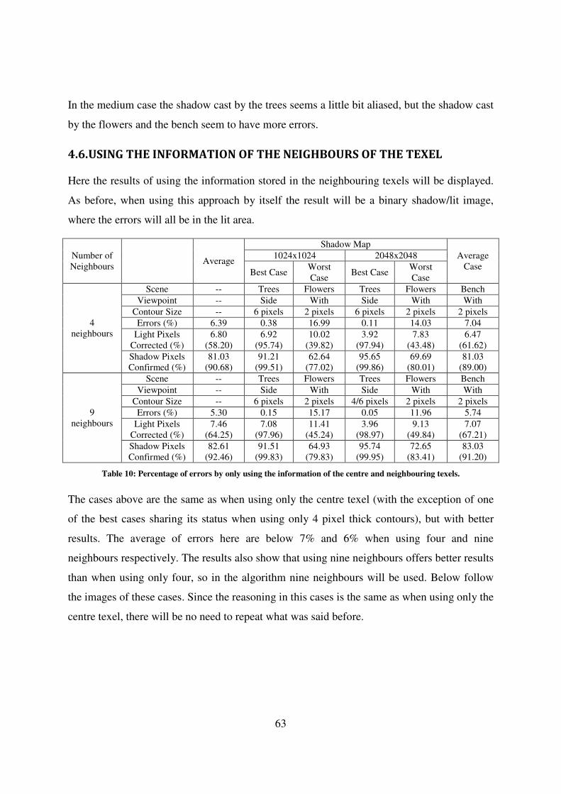
63
In the medium case the shadow cast by the trees seems a little bit aliased, but the shadow cast
by the flowers and the bench seem to have more errors.
4.6. USING THE INFORMATION OF THE NEIGHBOURS OF THE TEXEL
Here the results of using the information stored in the neighbouring texels will be displayed.
As before, when using this approach by itself the result will be a binary shadow/lit image,
where the errors will all be in the lit area.
Number of
Neighbours Average
Shadow Map
Average
Case
1024x1024 2048x2048
Best Case Worst
Case Best Case
Worst
Case
4
neighbours
Scene -- Trees Flowers Trees Flowers Bench
Viewpoint -- Side With Side With With
Contour Size -- 6 pixels 2 pixels 6 pixels 2 pixels 2 pixels
Errors (%) 6.39 0.38 16.99 0.11 14.03 7.04
Light Pixels
Corrected (%)
6.80
(58.20)
6.92
(95.74)
10.02
(39.82)
3.92
(97.94)
7.83
(43.48)
6.47
(61.62)
Shadow Pixels
Confirmed (%)
81.03
(90.68)
91.21
(99.51)
62.64
(77.02)
95.65
(99.86)
69.69
(80.01)
81.03
(89.00)
9
neighbours
Scene -- Trees Flowers Trees Flowers Bench
Viewpoint -- Side With Side With With
Contour Size -- 6 pixels 2 pixels 4/6 pixels 2 pixels 2 pixels
Errors (%) 5.30 0.15 15.17 0.05 11.96 5.74
Light Pixels
Corrected (%)
7.46
(64.25)
7.08
(97.96)
11.41
(45.24)
3.96
(98.97)
9.13
(49.84)
7.07
(67.21)
Shadow Pixels
Confirmed (%)
82.61
(92.46)
91.51
(99.83)
64.93
(79.83)
95.74
(99.95)
72.65
(83.41)
83.03
(91.20)
Table 10: Percentage of errors by only using the information of the centre and neighbouring texels.
The cases above are the same as when using only the centre texel (with the exception of one
of the best cases sharing its status when using only 4 pixel thick contours), but with better
results. The average of errors here are below 7% and 6% when using four and nine
neighbours respectively. The results also show that using nine neighbours offers better results
than when using only four, so in the algorithm nine neighbours will be used. Below follow
the images of these cases. Since the reasoning in this cases is the same as when using only the
centre texel, there will be no need to repeat what was said before.
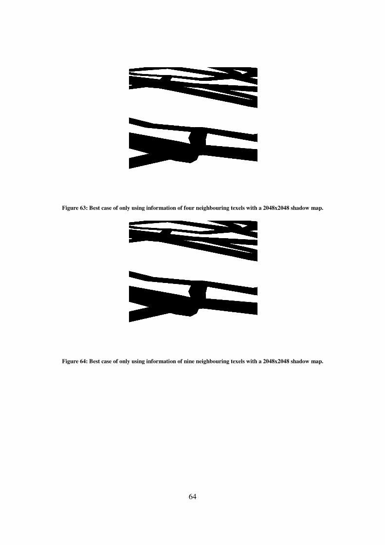
Figure 63: Best case of only using
Figure 64: Best case of only using
64
: Best case of only using information of four neighbouring texels with a 2048x2048 shadow map.
: Best case of only using information of nine neighbouring texels with a 2048x2048 shadow map.
with a 2048x2048 shadow map.
with a 2048x2048 shadow map.

Figure 65: Worst case of only using
Figure 66: Worst case of only
65
: Worst case of only using information of four neighbouring texels with a 2048x2048 shadow map.
: Worst case of only information of nine neighbouring texels with a 2048x2048 shadow map.
with a 2048x2048 shadow map.
with a 2048x2048 shadow map.
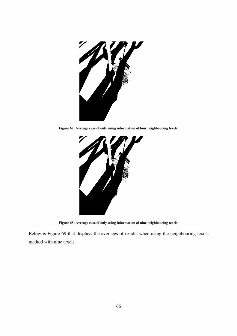
Figure 67: Average
Figure 68: Average
Below is Figure 69 that displays the averages of results when using th
method with nine texels.
66
Average case of only using information of four neighbouring texel
Average case of only using information of nine neighbouring texel
that displays the averages of results when using the neighbouring texels
neighbouring texels.
neighbouring texels.
e neighbouring texels
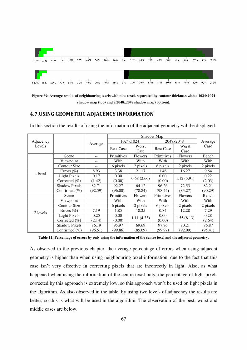
67
Figure 69: Average results of neighbouring texels with nine texels separated by contour thickness with a 1024x1024
shadow map (top) and a 2048x2048 shadow map (bottom).
4.7. USING GEOMETRIC ADJACENCY INFORMATION
In this section the results of using the information of the adjacent geometry will be displayed.
Adjacency
Levels Average
Shadow Map
Average
Case
1024x1024 2048x2048
Best Case Worst
Case Best Case
Worst
Case
1 level
Scene -- Primitives Flowers Primitives Flowers Bench
Viewpoint -- With With With With With
Contour Size -- 6 pixels 2 pixels 6 pixels 2 pixels 2 pixels
Errors (%) 8.93 3.38 21.17 1.46 16.27 9.64
Light Pixels
Corrected (%)
0.17
(1.42)
0.00
(0.00) 0.68 (2.66)
0.00
(0.00) 1.12 (5.91)
0.22
(2.03)
Shadow Pixels
Confirmed (%)
82.71
(92.59)
92.27
(96.00)
64.12
(78.84)
96.26
(98.44)
72.53
(83.27)
82.21
(90.29)
2 levels
Scene -- Primitives Flowers Primitives Flowers Bench
Viewpoint -- With With With With With
Contour Size -- 6 pixels 2 pixels 6 pixels 2 pixels 2 pixels
Errors (%) 7.19 1.85 18.25 0.84 12.28 7.29
Light Pixels
Corrected (%)
0.25
(2.14)
0.00
(0.00) 1.11 (4.33)
0.00
(0.00) 1.55 (8.13)
0.28
(2.64)
Shadow Pixels
Confirmed (%)
86.19
(96.51)
95.97
(99.86)
69.69
(85.69)
97.76
(99.97)
80.21
(92.09)
86.87
(95.41)
Table 11: Percentage of errors by only using the information of the centre texel and the adjacent geometry.
As observed in the previous chapter, the average percentage of errors when using adjacent
geometry is higher than when using neighbouring texel information, due to the fact that this
case isn’t very effective in correcting pixels that are incorrectly in light. Also, as what
happened when using the information of the centre texel only, the percentage of light pixels
corrected by this approach is extremely low, so this approach won’t be used on light pixels in
the algorithm. As also observed in the table, by using two levels of adjacency the results are
better, so this is what will be used in the algorithm. The observation of the best, worst and
middle cases are below.
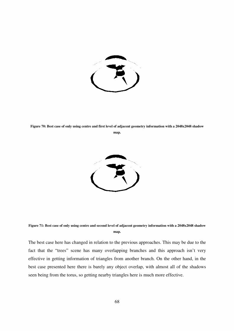
Figure 70: Best case of only using centre and first level of adja
Figure 71: Best case of only using centre and second level of adjacent geometry information with a 2048x2048 shadow
The best case here has changed in relation to the pre
fact that the “trees” scene has many overlapping branches and this approach isn’t very
effective in getting information of triangles from another branch. On the other hand, in the
best case presented here there is b
seen being from the torus, so getting nearby triangles here is much more effective.
68
: Best case of only using centre and first level of adjacent geometry information with a 2048x2048 shadow
map.
: Best case of only using centre and second level of adjacent geometry information with a 2048x2048 shadow
map.
The best case here has changed in relation to the previous approaches. This may be due to the
fact that the “trees” scene has many overlapping branches and this approach isn’t very
effective in getting information of triangles from another branch. On the other hand, in the
best case presented here there is barely any object overlap, with almost all of the shadows
o getting nearby triangles here is much more effective.
cent geometry information with a 2048x2048 shadow
: Best case of only using centre and second level of adjacent geometry information with a 2048x2048 shadow
vious approaches. This may be due to the
fact that the “trees” scene has many overlapping branches and this approach isn’t very
effective in getting information of triangles from another branch. On the other hand, in the
arely any object overlap, with almost all of the shadows
o getting nearby triangles here is much more effective.
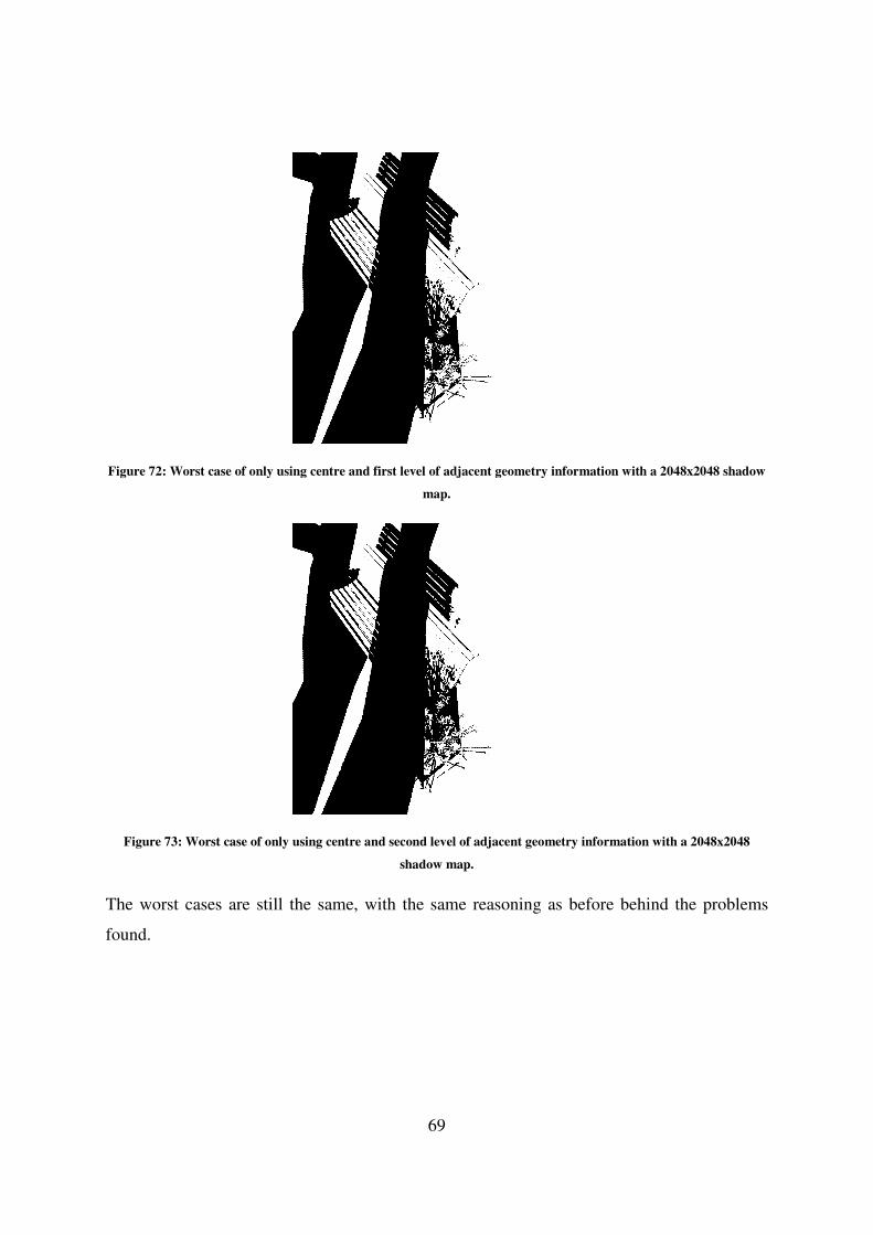
Figure 72: Worst case of only using centre and first level of adjacent geometry informat
Figure 73: Worst case of only using centre and second level of adjacent geometry information with a 2048x2048
The worst cases are still the same, with the same reasoning as before
found.
69
: Worst case of only using centre and first level of adjacent geometry information with a 2048x2048 shadow
map.
: Worst case of only using centre and second level of adjacent geometry information with a 2048x2048
shadow map.
The worst cases are still the same, with the same reasoning as before behind the problems
ion with a 2048x2048 shadow
: Worst case of only using centre and second level of adjacent geometry information with a 2048x2048
behind the problems

Figure 74: Average case of only using centre and first level of adjacent geometry information.
Figure 75: Average case of only using centre and second level of adjacent geomet
In the medium case the aliasing in the shadows cast by the trees is slightly visible, where in
the neighbouring texel results it has practically disappeared. The shadows cast by the bench
seem good, but in the shadows cast by the flowers so
And below Figure 76 shows the average results for the adjacent geometry approach when
used with two levels of adjacency.
70
case of only using centre and first level of adjacent geometry information.
case of only using centre and second level of adjacent geometry information.
In the medium case the aliasing in the shadows cast by the trees is slightly visible, where in
the neighbouring texel results it has practically disappeared. The shadows cast by the bench
seem good, but in the shadows cast by the flowers some errors can still be observed.
shows the average results for the adjacent geometry approach when
used with two levels of adjacency.
case of only using centre and first level of adjacent geometry information.
ry information.
In the medium case the aliasing in the shadows cast by the trees is slightly visible, where in
the neighbouring texel results it has practically disappeared. The shadows cast by the bench
me errors can still be observed.
shows the average results for the adjacent geometry approach when
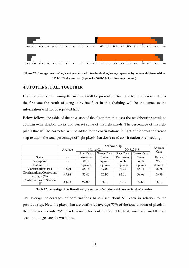
71
Figure 76: Average results of adjacent geometry with two levels of adjacency separated by contour thickness with a
1024x1024 shadow map (top) and a 2048x2048 shadow map (bottom).
4.8. PUTTING IT ALL TOGETHER
Here the results of chaining the methods will be presented. Since the texel coherence step is
the first one the result of using it by itself an in this chaining will be the same, so the
information will not be repeated here.
Below follows the table of the next step of the algorithm that uses the neighbouring texels to
confirm extra shadow pixels and correct some of the light pixels. The percentage of the light
pixels that will be corrected will be added to the confirmations in light of the texel coherence
step to attain the total percentage of light pixels that don’t need confirmation or correcting.
Average
Shadow Map Average
Case 1024x1024 2048x2048
Best Case Worst Case Best Case Worst Case
Scene -- Primitives Trees Primitives Trees Bench
Viewpoint -- With Against With With With
Contour Size -- 6 pixels 2 pixels 6 pixels 2 pixels 2 pixels
Confirmations (%) 75.04 88.16 49.09 94.27 58.71 76.36
Confirmations/Corrections
in Light (%) 65.98 85.43 26.97 92.50 39.68 66.79
Confirmations in Shadow
(%) 84.13 92.00 71.13 96.77 77.68 86.04
Table 12: Percentage of confirmations by algorithm after using neighbouring texel information.
The average percentages of confirmations have risen about 5% each in relation to the
previous step. Now the pixels that are confirmed average 75% of the total amount of pixels in
the contours, so only 25% pixels remain for confirmation. The best, worst and middle case
scenario images are shown below.
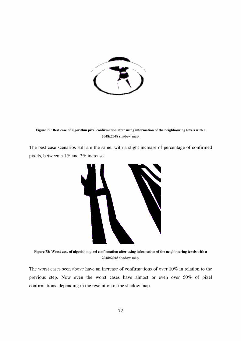
Figure 77: Best case of algorithm pixel confirmatio
The best case scenarios still are the same, with a slight increase of percentage of confirmed
pixels, between a 1% and 2% increase.
Figure 78: Worst case of algorithm pixel confirmation after using information of the neighbouring texels with a
The worst cases seen above have an increase of confirmations of over 10% in relation to the
previous step. Now even the worst cases have
confirmations, depending in the resolution
72
: Best case of algorithm pixel confirmation after using information of the neighbouring texels with a
2048x2048 shadow map.
The best case scenarios still are the same, with a slight increase of percentage of confirmed
pixels, between a 1% and 2% increase.
t case of algorithm pixel confirmation after using information of the neighbouring texels with a
2048x2048 shadow map.
The worst cases seen above have an increase of confirmations of over 10% in relation to the
previous step. Now even the worst cases have almost or even over 50% of pixel
confirmations, depending in the resolution of the shadow map.
n after using information of the neighbouring texels with a
The best case scenarios still are the same, with a slight increase of percentage of confirmed
t case of algorithm pixel confirmation after using information of the neighbouring texels with a
The worst cases seen above have an increase of confirmations of over 10% in relation to the
almost or even over 50% of pixel
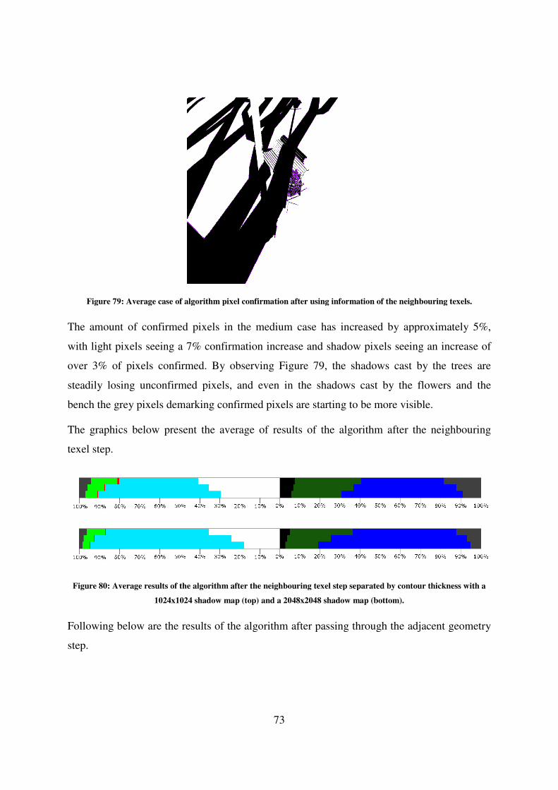
Figure 79: Average case of algorithm pixel confirmation after using information of the neighbouring texels.
The amount of confirmed pixels in the medium case has increased by approximately 5%,
with light pixels seeing a 7% confirmation increase and shadow pixels seeing an increase of
over 3% of pixels confirmed. By observing
steadily losing unconfirmed pixels, and even in the shadows cast by the flowers and the
bench the grey pixels demarking confirmed pixels are starting to be more visible.
The graphics below present the average of results of the algorithm after the neighbouring
texel step.
Figure 80: Average results of the algorithm after the neighbouring texel step
1024x1024 shadow map (t
Following below are the results of the algorithm after passing through the adjacent geometry
step.
73
case of algorithm pixel confirmation after using information of the neighbouring texels.
xels in the medium case has increased by approximately 5%,
with light pixels seeing a 7% confirmation increase and shadow pixels seeing an increase of
over 3% of pixels confirmed. By observing Figure 79, the shadows cast by the trees are
steadily losing unconfirmed pixels, and even in the shadows cast by the flowers and the
bench the grey pixels demarking confirmed pixels are starting to be more visible.
below present the average of results of the algorithm after the neighbouring
the algorithm after the neighbouring texel step separated by contour thickness with a
1024x1024 shadow map (top) and a 2048x2048 shadow map (bottom).
Following below are the results of the algorithm after passing through the adjacent geometry
case of algorithm pixel confirmation after using information of the neighbouring texels.
xels in the medium case has increased by approximately 5%,
with light pixels seeing a 7% confirmation increase and shadow pixels seeing an increase of
, the shadows cast by the trees are
steadily losing unconfirmed pixels, and even in the shadows cast by the flowers and the
bench the grey pixels demarking confirmed pixels are starting to be more visible.
below present the average of results of the algorithm after the neighbouring
separated by contour thickness with a
op) and a 2048x2048 shadow map (bottom).
Following below are the results of the algorithm after passing through the adjacent geometry
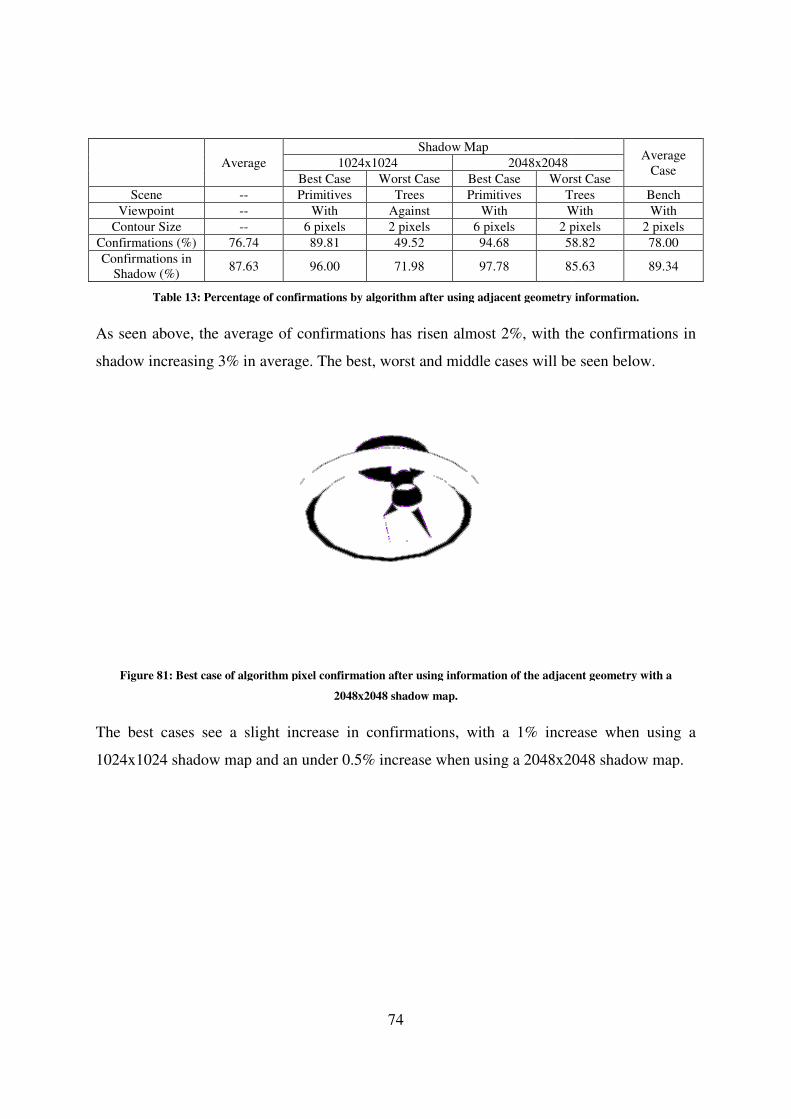
Average
Scene --
Viewpoint --
Contour Size --
Confirmations (%) 76.74
Confirmations in
Shadow (%) 87.63
Table 13: Percentage of confirmations by algorithm after using adjacent geometry information.
As seen above, the average of confirmations has risen almost 2%, with the confirmations in
shadow increasing 3% in average.
Figure 81: Best case of algorithm pixel confirmation after using information of the adjacent geometry with a
The best cases see a slight increase in
1024x1024 shadow map and an under 0.5% increase when using a 2048x2048 shadow map.
74
Shadow Map
1024x1024 2048x2048
Best Case Worst Case Best Case Worst Case
Primitives Trees Primitives Trees
With Against With With
6 pixels 2 pixels 6 pixels 2 pixels
89.81 49.52 94.68 58.82
96.00 71.98 97.78 85.63
: Percentage of confirmations by algorithm after using adjacent geometry information.
As seen above, the average of confirmations has risen almost 2%, with the confirmations in
shadow increasing 3% in average. The best, worst and middle cases will be seen below.
: Best case of algorithm pixel confirmation after using information of the adjacent geometry with a
2048x2048 shadow map.
The best cases see a slight increase in confirmations, with a 1% increase when using a
1024x1024 shadow map and an under 0.5% increase when using a 2048x2048 shadow map.
Average
Case
Worst Case
Trees Bench
With With
2 pixels 2 pixels
58.82 78.00
85.63 89.34
: Percentage of confirmations by algorithm after using adjacent geometry information.
As seen above, the average of confirmations has risen almost 2%, with the confirmations in
The best, worst and middle cases will be seen below.
: Best case of algorithm pixel confirmation after using information of the adjacent geometry with a
confirmations, with a 1% increase when using a
1024x1024 shadow map and an under 0.5% increase when using a 2048x2048 shadow map.
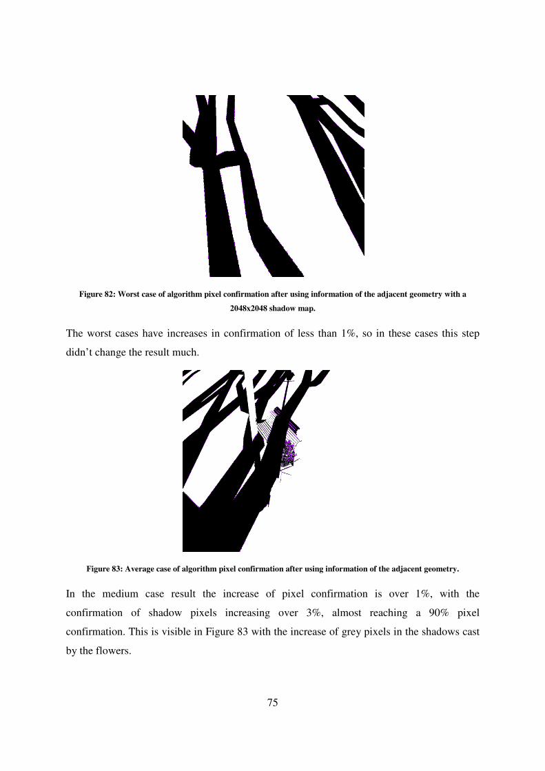
Figure 82: Worst case of algorithm pixel confirmation after using information of the adjacent geome
The worst cases have increases in confirmation of less than 1%, so in these cases this step
didn’t change the result much.
Figure 83: Average case of algorithm pixel confirmation after using infor
In the medium case result the increase of pixel confirmation is over 1%, with the
confirmation of shadow pixels increasing over 3%, almost reaching a 90% pixel
confirmation. This is visible in
by the flowers.
75
: Worst case of algorithm pixel confirmation after using information of the adjacent geome
2048x2048 shadow map.
The worst cases have increases in confirmation of less than 1%, so in these cases this step
didn’t change the result much.
case of algorithm pixel confirmation after using information of the adjacent geometry.
In the medium case result the increase of pixel confirmation is over 1%, with the
confirmation of shadow pixels increasing over 3%, almost reaching a 90% pixel
confirmation. This is visible in Figure 83 with the increase of grey pixels in the shadows cast
: Worst case of algorithm pixel confirmation after using information of the adjacent geometry with a
The worst cases have increases in confirmation of less than 1%, so in these cases this step
mation of the adjacent geometry.
In the medium case result the increase of pixel confirmation is over 1%, with the
confirmation of shadow pixels increasing over 3%, almost reaching a 90% pixel
with the increase of grey pixels in the shadows cast
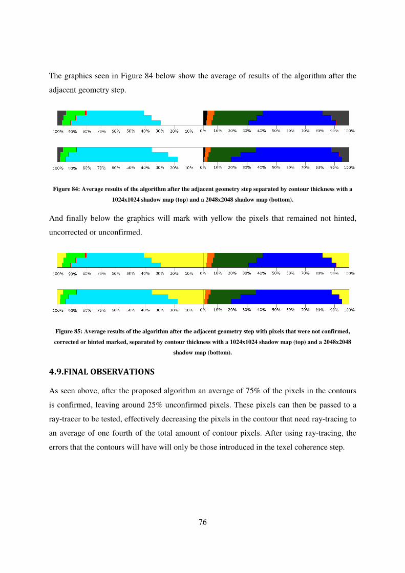
76
The graphics seen in Figure 84 below show the average of results of the algorithm after the
adjacent geometry step.
Figure 84: Average results of the algorithm after the adjacent geometry step separated by contour thickness with a
1024x1024 shadow map (top) and a 2048x2048 shadow map (bottom).
And finally below the graphics will mark with yellow the pixels that remained not hinted,
uncorrected or unconfirmed.
Figure 85: Average results of the algorithm after the adjacent geometry step with pixels that were not confirmed,
corrected or hinted marked, separated by contour thickness with a 1024x1024 shadow map (top) and a 2048x2048
shadow map (bottom).
4.9. FINAL OBSERVATIONS
As seen above, after the proposed algorithm an average of 75% of the pixels in the contours
is confirmed, leaving around 25% unconfirmed pixels. These pixels can then be passed to a
ray-tracer to be tested, effectively decreasing the pixels in the contour that need ray-tracing to
an average of one fourth of the total amount of contour pixels. After using ray-tracing, the
errors that the contours will have will only be those introduced in the texel coherence step.
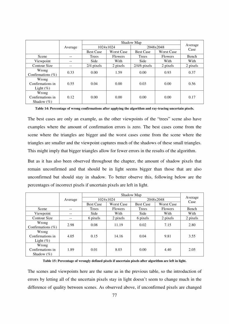
77
Average
Shadow Map Average
Case 1024x1024 2048x2048
Best Case Worst Case Best Case Worst Case
Scene -- Trees Flowers Trees Flowers Bench
Viewpoint -- Side With Side With With
Contour Size -- 2/4 pixels 2 pixels 2/4/6 pixels 2 pixels 2 pixels
Wrong
Confirmations (%) 0.33 0.00 1.59 0.00 0.93 0.37
Wrong
Confirmations in
Light (%)
0.55 0.04 0.00 0.03 0.00 0.56
Wrong
Confirmations in
Shadow (%)
0.12 0.00 0.00 0.00 0.00 0.17
Table 14: Percentage of wrong confirmations after applying the algorithm and ray-tracing uncertain pixels.
The best cases are only an example, as the other viewpoints of the “trees” scene also have
examples where the amount of confirmation errors is zero. The best cases come from the
scene where the triangles are bigger and the worst cases come from the scene where the
triangles are smaller and the viewpoint captures much of the shadows of these small triangles.
This might imply that bigger triangles allow for fewer errors in the results of the algorithm.
But as it has also been observed throughout the chapter, the amount of shadow pixels that
remain unconfirmed and that should be in light seems bigger than those that are also
unconfirmed but should stay in shadow. To better observe this, following below are the
percentages of incorrect pixels if uncertain pixels are left in light.
Average
Shadow Map Average
Case 1024x1024 2048x2048
Best Case Worst Case Best Case Worst Case
Scene -- Trees Flowers Trees Flowers Bench
Viewpoint -- Side With Side With With
Contour Size -- 6 pixels 2 pixels 6 pixels 2 pixels 2 pixels
Wrong
Confirmations (%) 2.98 0.08 11.19 0.02 7.15 2.80
Wrong
Confirmations in
Light (%)
4.05 0.15 14.16 0.04 9.81 3.55
Wrong
Confirmations in
Shadow (%)
1.89 0.01 8.03 0.00 4.40 2.05
Table 15: Percentage of wrongly defined pixels if uncertain pixels after algorithm are left in light.
The scenes and viewpoints here are the same as in the previous table, so the introduction of
errors by letting all of the uncertain pixels stay in light doesn’t seem to change much in the
difference of quality between scenes. As observed above, if unconfirmed pixels are changed
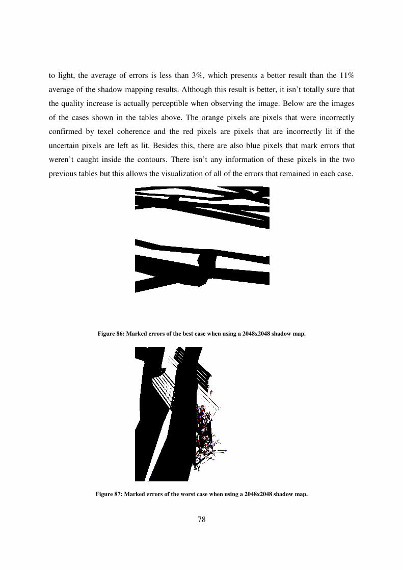
to light, the average of errors is less than 3%, which presents a better result than the 11%
average of the shadow mapping results. Although this result is better, it isn’t totally sure that
the quality increase is actually perceptible when observing the image.
of the cases shown in the tables above. The orange pixels are pixels that were incorrectly
confirmed by texel coherence and the red pixels are pixels that are incorrectly lit if
uncertain pixels are left as lit. Besides this, there are also blue pixels that mark errors that
weren’t caught inside the contours. There isn’t any information of these pixels in the two
previous tables but this allows
Figure 86: Marked errors of the best case when using a 2048x2048 shadow map.
Figure 87: Marked errors of the worst case when using a 2048x2048 shadow map.
78
the average of errors is less than 3%, which presents a better result than the 11%
average of the shadow mapping results. Although this result is better, it isn’t totally sure that
ncrease is actually perceptible when observing the image. Below are the images
of the cases shown in the tables above. The orange pixels are pixels that were incorrectly
confirmed by texel coherence and the red pixels are pixels that are incorrectly lit if
uncertain pixels are left as lit. Besides this, there are also blue pixels that mark errors that
weren’t caught inside the contours. There isn’t any information of these pixels in the two
previous tables but this allows the visualization of all of the errors that remained in each case.
: Marked errors of the best case when using a 2048x2048 shadow map.
: Marked errors of the worst case when using a 2048x2048 shadow map.
the average of errors is less than 3%, which presents a better result than the 11%
average of the shadow mapping results. Although this result is better, it isn’t totally sure that
Below are the images
of the cases shown in the tables above. The orange pixels are pixels that were incorrectly
confirmed by texel coherence and the red pixels are pixels that are incorrectly lit if the
uncertain pixels are left as lit. Besides this, there are also blue pixels that mark errors that
weren’t caught inside the contours. There isn’t any information of these pixels in the two
errors that remained in each case.
: Marked errors of the best case when using a 2048x2048 shadow map.
: Marked errors of the worst case when using a 2048x2048 shadow map.

Figure
79
Figure 88: Marked errors of the average case.

80
81
5. CONCLUSIONS AND FUTURE WORK
Shadow mapping is probably the most used algorithm to compute shadows in real time. The
performance of the algorithm is very high, but it has severe issues that cause aliased shadow
contours.
Ray-tracer on the other hand is capable of producing pixel perfect shadows. Yet, from a
performance point of view is not as friendly.
Shadow mapping has been a deeply studied algorithm, with many researchers proposing
improvements to its quality without compromising its efficiency. Most of the new approaches
focus only on the original method, or variations thereof.
Nevertheless some researchers have developed hybrid methods, combining shadow mapping
with ray-tracing. The main goal of these hybrid methods is to obtain visual results that closely
match ray-traced shadows, while not fully compromising performance. The main approach is
therefore to use a first pass with shadow mapping and use this information to determine
which pixels should be ray-traced. Ideally this set of pixels should be a small subset of the
original rendered image.
One of these methods focuses on the contours of the shadows, and uses texel coherence to
determine if a pixel should be ray-traced. Pixels that have texel coherence are those that
project onto a texel which has an identical shadow status to the neighbouring texels. For
instance if a pixel projects onto a texel which indicates a shadow, and the neighbouring texels
also indicate a shadow, then said pixel has texel coherence.
This work established the theme for this thesis. The main goals are to quantify the
assumptions being made on the referred work, and to discover other methods to reduce the
subset of pixels that require ray-tracing, i.e. those whose shadow status can’t be determined
for sure using only the shadow map information.
As for the first goal, it was verified that in average the vast majority of shadow mapping
errors are indeed in the contour areas of the shadows in the rendered image. As for using
texel coherence as a hint for the shadow status it was verified that in average roughly half of
the contour pixels have texel coherence, with only a small percentage of those being

82
incorrectly hinted. However it was also found that the percentage varies wildly with the
scene, achieving values as low as less than 3% of the contour pixels.
The second goal was to reduce the subset of pixels that require ray-tracing. To achieve this a
number of techniques that significantly reduce the size of this subset have been developed.
These methods rely solely on the information about which triangles are recorded on the
shadow map, and one of them also uses geometric adjacency information.
The techniques are able to confirm pixels in shadow and/or detect incorrect pixels in light.
Note that it is not possible to correct a pixel in shadow with this limited information, since
that would imply a guarantee that there is no triangle in the scene that causes a shadow to the
said pixel. The methods work on very limited information, having access to only the triangles
that are recorder on the shadow map, and geometric adjacency information, hence no
assurances can be made regarding the remaining triangles. Similarly, for a pixel originally in
light it is not possible to confirm it, as that would imply a guarantee that no triangle in the
scene intersects the light ray.
The first technique is to determine if the light ray for that pixel intersects the triangle which
covered the respective texel. For pixels in shadow if an intersection occurs then the pixel is
definitely in shadow, otherwise the test is not conclusive. For pixels in light, it is usually the
case that the triangle that covers the texel is further away from the light than the said pixel.
Special situations where this is not the case have been properly identified but their occurrence
is too rare to compensate the effort.
Extending this test to neighbouring texels provides potentially more triangles to test, with the
upper limit of as many triangles as neighbouring texels. With this approach not only a larger
set of confirmed pixels in shadow can be obtained but also a good amount of pixels
erroneously in light can be corrected.
The adjacency information allows to further confirmation of pixels in shadow, but it is not
very successful at correcting pixels originally in light.
Since each method has its strengths, a pipeline was proposed where in each stage the input
are the pixels that were not confirmed/correct in the previous stages. The lightest methods

83
were placed on the beginning of the pipeline to limit the heavier methods to as few pixels as
possible.
While texel coherence is not capable of actually confirming/correcting pixels it does provide
a strong hint regarding the shadow status, and the number of pixels hinted can be very
significant. Under this context, and since this method is as fast as shadow mapping itself,
texel coherence could be used in a dynamic approach when the frame rate drops below a
certain threshold.
The final number of pixels that remain unconfirmed/uncorrected is significantly reduced with
this pipeline when compared to texel coherence per se hence the goals of this work have been
achieved.
As further work we would like to implement the above mentioned pipeline as a GPU
solution, using only shaders, and evaluate its performance. Ray-tracing the
unconfirmed/uncorrected pixels could be performed for instance with OptiX. A full
evaluation performance could then be completed to evaluate the merits of the proposed
solution.

84
85
6. BIBLIOGRAPHY
Agrawala, M., Ramamoorthi, R., Heirich, A., & Moll, L. (2000). Efficient Image-Based
Methods for Rendering Soft Shadows. Proceedings of SIGGRAPH, Computer Graphics
Proceedings, Anual Conference Series (pp. 375-384). ACM.
Annen, T., Mertens, T., Bekaert, P., Seidel, H., & Kautz, J. (2007). Convolution Shadow
Maps. Rendering Techniques 2007, volume 1 of Eurographics/ACMSIGGRAPH Symposium
Proceedings (pp. 51-60). Eurographics.
Annen, T., Mertens, T., Seidel, H., Flerackers, E., & Kautz, J. (2008). Exponential Shadow
Maps. Proceedings of Graphics Interface 2008 (pp. 155-161). Ontario, Canada: Canadian
Information Processing Society.
Barbec, S., Annen, T., & Seidel, H. (2002). Practical Shadow Mapping.
Beister, M., Ernst, M., & Stamminger, M. (2005). A Hybrid GPU-CPU Renderer. VMV 2005
.
Chan, E., & Durand, F. (2004). An Efficient Hybrid Shadow Rendering Algorithm.
Proceedings of the Eurographics Symposium on Rendering (pp. 185-195). Norrköping,
Sweden: Eurographics Association.
Dempski, K., & Viale, E. (2004). Advanced Lighting and Materials with Shaders. Wordware
Publishing Inc.
Donnelly, W., & Lauritzen, A. (2006). Variance Shadow Maps. ID3.
Fernando, R., Fernandez, S., Bala, K., & Greenberg, D. P. (2001). Adaptive Shadow Maps.
Proceedings of ACM SIGGRAPH 2001, ACM Press/ACM SIGGRAPH, Computer Graphics
Proceedings, Annual Conference Series (pp. 387-390). ACM.
Hertel, S., Hormann, K., & Westermann, R. (2009). A hybrid GPU rendering for alias-free
hard shadows. In D. Ebert, & J. Krüger (Ed.), Eurographics 2009 Areas Papers (pp. 59-66).
Müchen, Germany: Eurographics Association.
Jensen, H. W. (2001). Realistic Image Synthesis Using Photon Mapping. A. K. Peters.
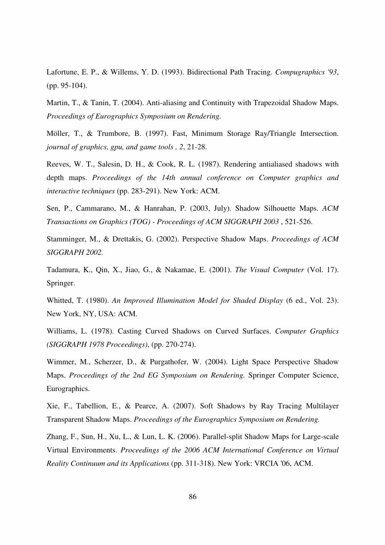
86
Lafortune, E. P., & Willems, Y. D. (1993). Bidirectional Path Tracing. Compugraphics '93,
(pp. 95-104).
Martin, T., & Tanin, T. (2004). Anti-aliasing and Continuity with Trapezoidal Shadow Maps.
Proceedings of Eurographics Symposium on Rendering.
Möller, T., & Trumbore, B. (1997). Fast, Minimum Storage Ray/Triangle Intersection.
journal of graphics, gpu, and game tools , 2, 21-28.
Reeves, W. T., Salesin, D. H., & Cook, R. L. (1987). Rendering antialiased shadows with
depth maps. Proceedings of the 14th annual conference on Computer graphics and
interactive techniques (pp. 283-291). New York: ACM.
Sen, P., Cammarano, M., & Hanrahan, P. (2003, July). Shadow Silhouette Maps. ACM
Transactions on Graphics (TOG) - Proceedings of ACM SIGGRAPH 2003 , 521-526.
Stamminger, M., & Drettakis, G. (2002). Perspective Shadow Maps. Proceedings of ACM
SIGGRAPH 2002.
Tadamura, K., Qin, X., Jiao, G., & Nakamae, E. (2001). The Visual Computer (Vol. 17).
Springer.
Whitted, T. (1980). An Improved Illumination Model for Shaded Display (6 ed., Vol. 23).
New York, NY, USA: ACM.
Williams, L. (1978). Casting Curved Shadows on Curved Surfaces. Computer Graphics
(SIGGRAPH 1978 Proceedings), (pp. 270-274).
Wimmer, M., Scherzer, D., & Purgathofer, W. (2004). Light Space Perspective Shadow
Maps. Proceedings of the 2nd EG Symposium on Rendering. Springer Computer Science,
Eurographics.
Xie, F., Tabellion, E., & Pearce, A. (2007). Soft Shadows by Ray Tracing Multilayer
Transparent Shadow Maps. Proceedings of the Eurographics Symposium on Rendering.
Zhang, F., Sun, H., Xu, L., & Lun, L. K. (2006). Parallel-split Shadow Maps for Large-scale
Virtual Environments. Proceedings of the 2006 ACM International Conference on Virtual
Reality Continuum and its Applications (pp. 311-318). New York: VRCIA '06, ACM.
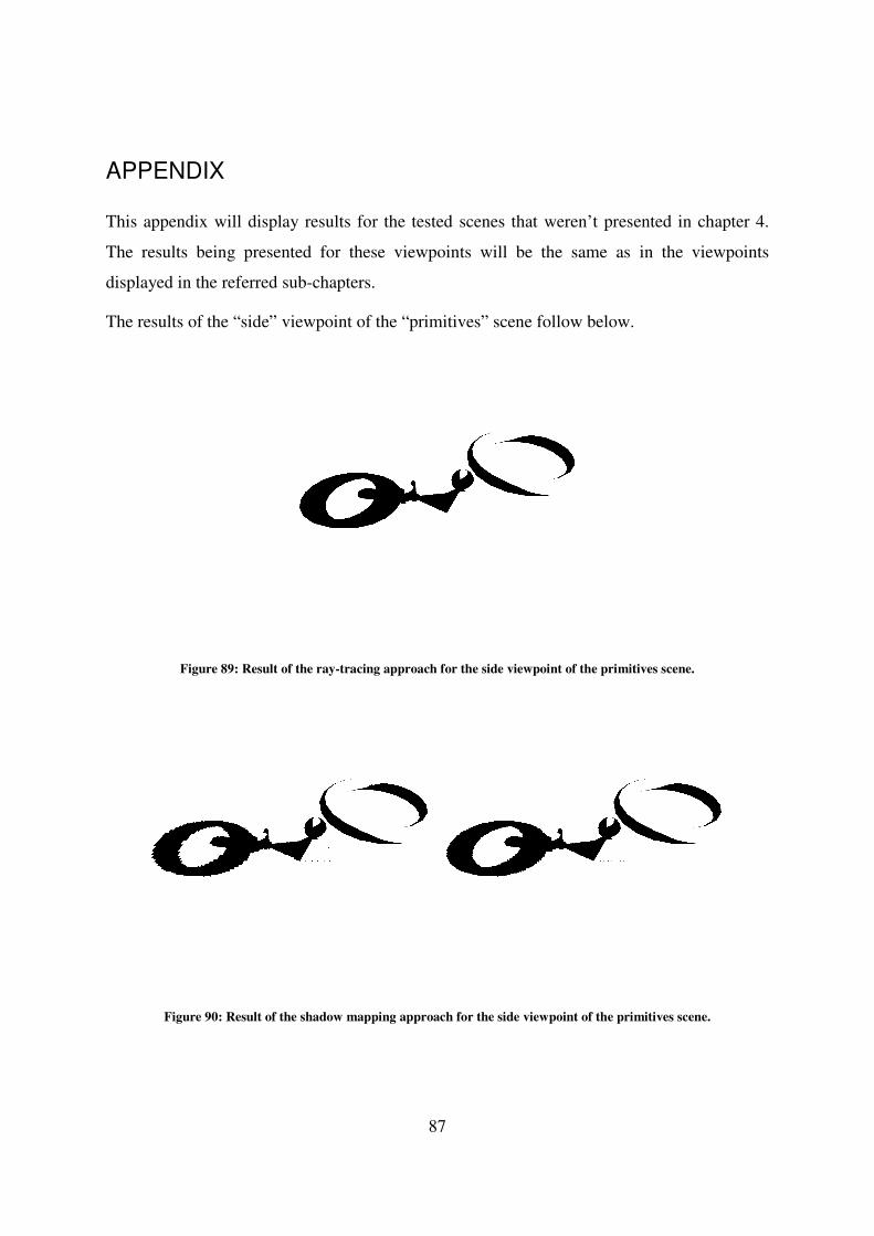
APPENDIX
This appendix will display results
The results being presented
displayed in the referred sub-chapte
The results of the “side” viewpoint of the
Figure 89: Result of the ray
Figure 90: Result of the shadow mapping approach for the
87
This appendix will display results for the tested scenes that weren’t presented in
The results being presented for these viewpoints will be the same as in
chapters.
viewpoint of the “primitives” scene follow below.
: Result of the ray-tracing approach for the side viewpoint of the primitives scene.
: Result of the shadow mapping approach for the side viewpoint of the primitives
that weren’t presented in chapter 4.
will be the same as in the viewpoints
scene follow below.
tracing approach for the side viewpoint of the primitives scene.
primitives scene.
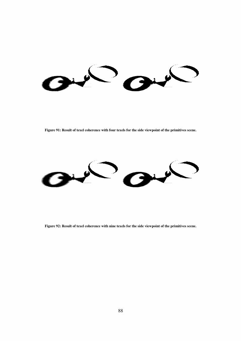
Figure 91: Result of texel coherence with four texels for
Figure 92: Result of texel coherence with nine texels for
88
: Result of texel coherence with four texels for the side viewpoint of the primitives scene
: Result of texel coherence with nine texels for the side viewpoint of the primitives scene
the side viewpoint of the primitives scene.
the side viewpoint of the primitives scene.
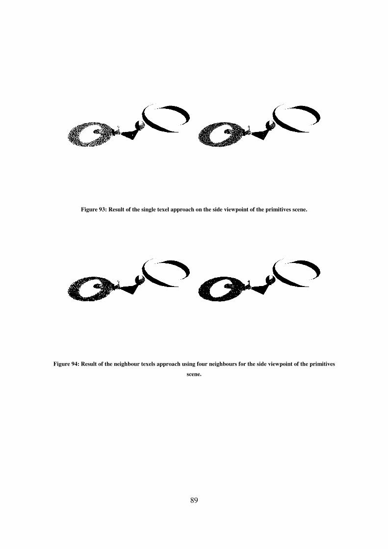
89
Figure 93: Result of the single texel approach on the side viewpoint of the primitives scene.
Figure 94: Result of the neighbour texels approach using four neighbours for the side viewpoint of the primitives
scene.
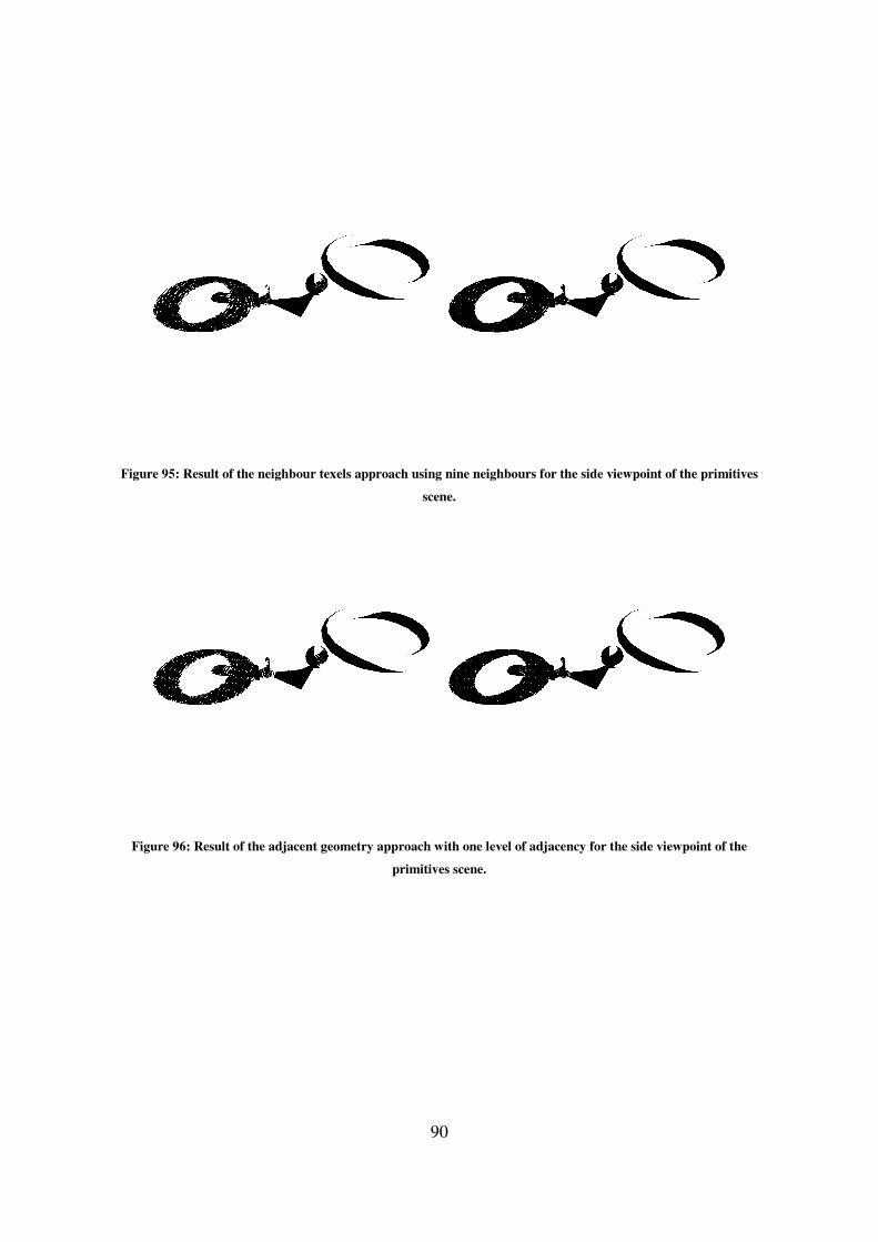
90
Figure 95: Result of the neighbour texels approach using nine neighbours for the side viewpoint of the primitives
scene.
Figure 96: Result of the adjacent geometry approach with one level of adjacency for the side viewpoint of the
primitives scene.

Figure 97: Result of the adjacent geometry
Figure 98: Result of the algorithm with a six pixel thick contour and a 2048x2048 resolution shadow map
91
adjacent geometry approach with two levels of adjacency for the side viewpoint of the
primitives scene.
with a six pixel thick contour and a 2048x2048 resolution shadow map
viewpoint of the primitives scene.
the side viewpoint of the
with a six pixel thick contour and a 2048x2048 resolution shadow map for the side
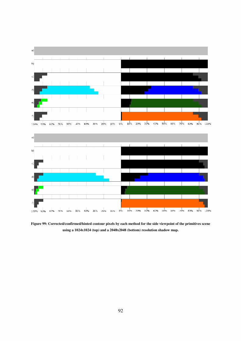
92
Figure 99: Corrected/confirmed/hinted contour pixels by each method for the side viewpoint of the primitives scene
using a 1024x1024 (top) and a 2048x2048 (bottom) resolution shadow map.
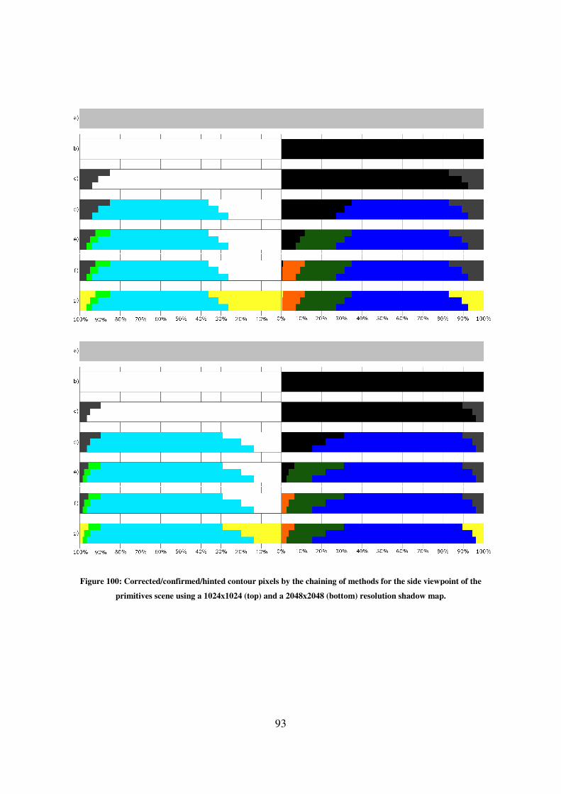
Figure 100: Corrected/confirmed/hinted contour pixels by
primitives scene using a 1024x1024 (
93
: Corrected/confirmed/hinted contour pixels by the chaining of methods for the side viewpoint of the
primitives scene using a 1024x1024 (top) and a 2048x2048 (bottom) resolution shadow map.
for the side viewpoint of the
) resolution shadow map.

94
Shadow Map
Resolution Approach
Contour Thickness
Two Pixels Four Pixels Six Pixels Whole Image
1024x1024
Pixels in
Contour 11000 21482 31683 1048576
Shadow Map 1769 (16.08%) 2138 (9.95%) 2164 (6.83%) 2164 (0.21%)
Single Texel 1973 (17.94%) 3418 (15.91%) 4458 (14.07%) 17500 (1.67%)
Neighbour
Texels
(4Neighbours)
1384 (12.58%) 2256 (10.50%) 2790 (8.81%) 7345 (0.70%)
Neighbour
Texels (9
Neighbours)
1086 (9.87%) 1729 (8.05%) 2077 (6.56%) 5004 (0.48%)
Adjacent
Geometry (One
Level)
1401 (12.74%) 2068 (9.63%) 2403 (7.58%) 4812 (0.46%)
Adjacent
Geometry
(Two Level)
903 (8.21%) 1129 (5.26%) 1184 (3.74%) 1290 (0.12%)
2048x2048
Pixels in
Contour 10750 21022 31047 1048576
Shadow Map 1111 (10.33%) 1123 (5.34%) 1123 (3.62%) 1123 (0.11%)
Single Texel 1452 (13.51%) 2136 (10.16%) 2833 (9.12%) 9989 (0.95%)
Neighbour
Texels (4
Neighbours)
796 (7.40%) 1027 (4.89%) 1231 (3.96%) 2486 (0.24%)
Neighbour
Texels (9
Neighbours)
608 (5.66%) 733 (3.49%) 858 (2.76%) 1620 (0.15%)
Adjacent
Geometry (One
Level)
855 (7.95%) 990 (4.71%) 1115 (3.59%) 1754 (0.17%)
Adjacent
Geometry
(Two Level)
609 (5.67%) 630 (3.00%) 638 (2.05%) 682 (0.07%)
Table 16: Difference between the approaches that use ray-tracing and the actual ray-tracer for the side viewpoint of
the primitives scene.
Shadow Map Resolution Contour Thickness
Two Pixels Four Pixels Six Pixels
1024x1024 1769 of 2164 (81.75%) 2138 of 2164 (98.80%) 2164 of 2164 (100.00%)
2048x2048 1111 of 1123 (98.93%) 1123 of 1123 (100.00%) 1123 of 1123 (100.00%)
Table 17: Wrongly defined pixels in the shadow mapping result which are inside the contour in the side viewpoint of
the primitives scene.
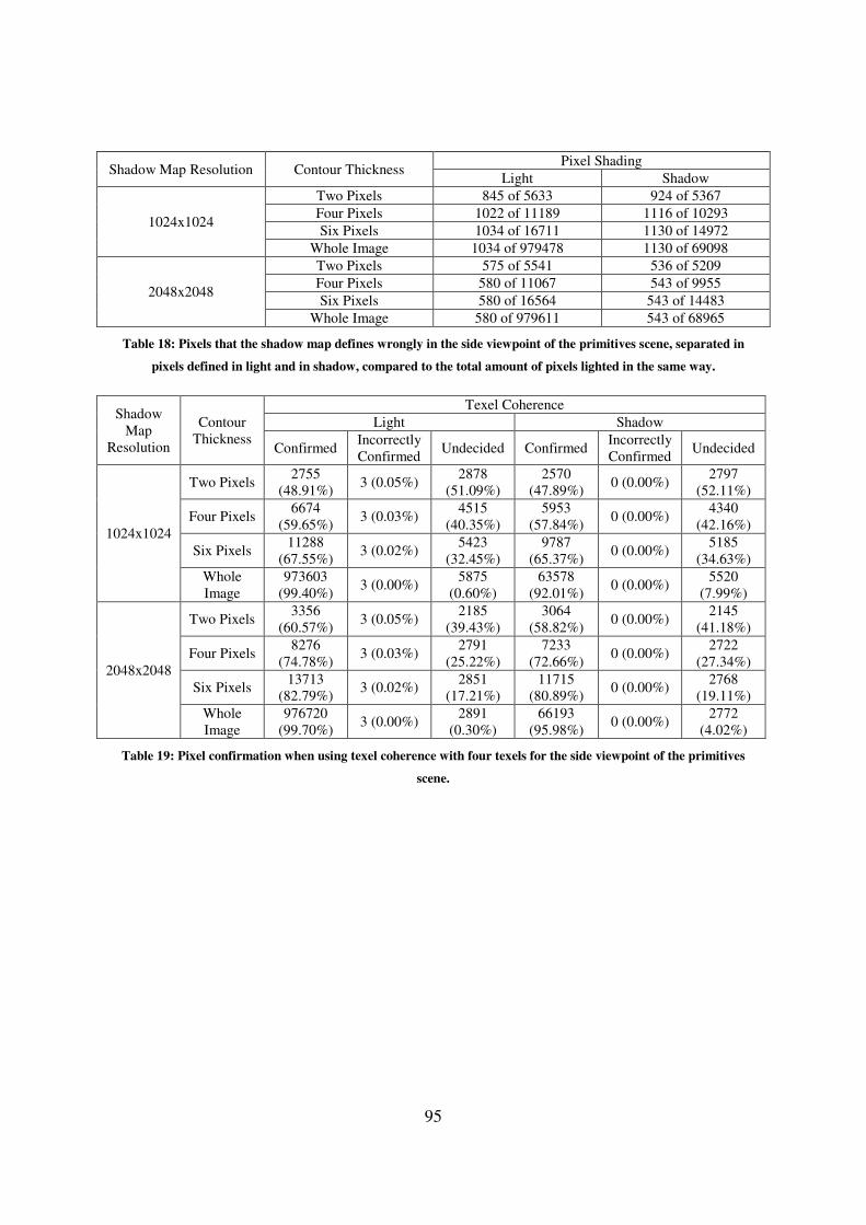
95
Shadow Map Resolution Contour Thickness Pixel Shading
Light Shadow
1024x1024
Two Pixels 845 of 5633 924 of 5367
Four Pixels 1022 of 11189 1116 of 10293
Six Pixels 1034 of 16711 1130 of 14972
Whole Image 1034 of 979478 1130 of 69098
2048x2048
Two Pixels 575 of 5541 536 of 5209
Four Pixels 580 of 11067 543 of 9955
Six Pixels 580 of 16564 543 of 14483
Whole Image 580 of 979611 543 of 68965
Table 18: Pixels that the shadow map defines wrongly in the side viewpoint of the primitives scene, separated in
pixels defined in light and in shadow, compared to the total amount of pixels lighted in the same way.
Shadow
Map
Resolution
Contour
Thickness
Texel Coherence
Light Shadow
Confirmed Incorrectly
Confirmed Undecided Confirmed
Incorrectly
Confirmed Undecided
1024x1024
Two Pixels 2755
(48.91%) 3 (0.05%)
2878
(51.09%)
2570
(47.89%) 0 (0.00%)
2797
(52.11%)
Four Pixels 6674
(59.65%) 3 (0.03%)
4515
(40.35%)
5953
(57.84%) 0 (0.00%)
4340
(42.16%)
Six Pixels 11288
(67.55%) 3 (0.02%)
5423
(32.45%)
9787
(65.37%) 0 (0.00%)
5185
(34.63%)
Whole
Image
973603
(99.40%) 3 (0.00%)
5875
(0.60%)
63578
(92.01%) 0 (0.00%)
5520
(7.99%)
2048x2048
Two Pixels 3356
(60.57%) 3 (0.05%)
2185
(39.43%)
3064
(58.82%) 0 (0.00%)
2145
(41.18%)
Four Pixels 8276
(74.78%) 3 (0.03%)
2791
(25.22%)
7233
(72.66%) 0 (0.00%)
2722
(27.34%)
Six Pixels 13713
(82.79%) 3 (0.02%)
2851
(17.21%)
11715
(80.89%) 0 (0.00%)
2768
(19.11%)
Whole
Image
976720
(99.70%) 3 (0.00%)
2891
(0.30%)
66193
(95.98%) 0 (0.00%)
2772
(4.02%)
Table 19: Pixel confirmation when using texel coherence with four texels for the side viewpoint of the primitives
scene.
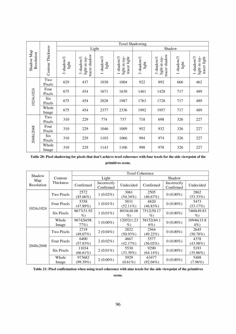
96
Sh
ado
w M
ap
Res
olu
tio
n
Co
nto
ur
Th
ick
nes
s Texel Shadowing
Light Shadow
3 s
had
ow
/1
lig
ht
3 s
had
ow
/1
lig
ht
in r
ay-
trac
er s
had
ow
1 s
had
ow
/3
lig
ht
1 s
had
ow
/3
lig
ht
in r
ay-
trac
er l
igh
t
3 s
had
ow
/1
lig
ht
3 s
had
ow
/1
lig
ht
in r
ay-
trac
er s
had
ow
1 s
had
ow
/3
lig
ht
1 s
had
ow
/3
lig
ht
in r
ay-
trac
er l
igh
t
10
24x
102
4
Two
Pixels 629 437 1038 1004 922 892 666 462
Four
Pixels 675 454 1671 1630 1461 1428 717 489
Six
Pixels 675 454 2028 1987 1763 1728 717 489
Whole
Image 675 454 2377 2336 1992 1957 717 489
20
48x
204
8
Two
Pixels 310 229 774 737 718 698 326 227
Four
Pixels 310 229 1046 1009 952 932 326 227
Six
Pixels 310 229 1103 1066 994 974 326 227
Whole
Image 310 229 1143 1106 998 978 326 227
Table 20: Pixel shadowing for pixels that don’t achieve texel coherence with four texels for the side viewpoint of the
primitives scene.
Shadow
Map
Resolution
Contour
Thickness
Texel Coherence
Light Shadow
Confirmed Incorrectly
Confirmed Undecided Confirmed
Incorrectly
Confirmed Undecided
1024x1024
Two Pixels 2572
(45.66%) 1 (0.02%)
3061
(54.34%)
2505
(46.67%) 0 (0.00%)
2862
(53.33%)
Four Pixels 5358
(47.89%) 1 (0.01%)
5831
(52.11%)
4820
(46.83%) 0 (0.00%)
5473
(53.17%)
Six Pixels 8677(51.92
%) 1 (0.01%)
8034(48.08
%)
7512(50.17
%) 0 (0.00%)
7460(49.83
%)
Whole
Image
967426(98.
77%) 1 (0.00%)
12052(1.23
%)
58152(84.1
6%) 0 (0.00%)
10946(15.8
4%)
2048x2048
Two Pixels 2719
(49.07%) 2 (0.04%)
2822
(50.93%)
2564
(49.22%) 0 (0.00%)
2645
(50.78%)
Four Pixels 6400
(57.83%) 2 (0.02%)
4667
(42.17%)
5577
(56.02%) 0 (0.00%)
4378
(43.98%)
Six Pixels 11034
(66.61%) 2 (0.01%)
5530
(33.39%)
9290
(64.14%) 0 (0.00%)
5193
(35.86%)
Whole
Image
973682
(99.39%) 2 (0.00%)
5929
(0.61%)
63477
(92.04%) 0 (0.00%)
5488
(7.96%)
Table 21: Pixel confirmation when using texel coherence with nine texels for the side viewpoint of the primitives
scene.
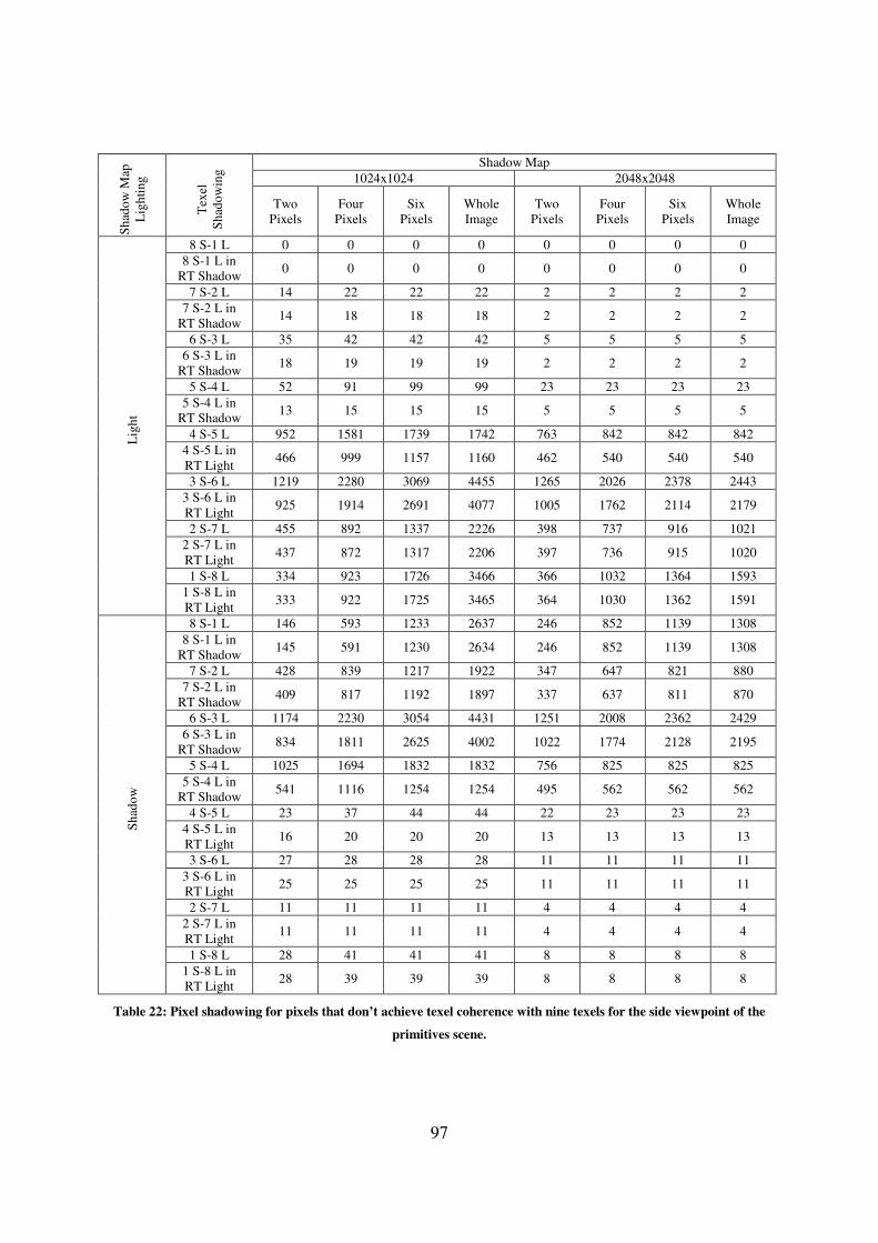
97
Sh
ado
w M
ap
Lig
hti
ng
Tex
el
Sh
ado
win
g Shadow Map
1024x1024 2048x2048
Two
Pixels
Four
Pixels
Six
Pixels
Whole
Image
Two
Pixels
Four
Pixels
Six
Pixels
Whole
Image
Lig
ht
8 S-1 L 0 0 0 0 0 0 0 0
8 S-1 L in
RT Shadow 0 0 0 0 0 0 0 0
7 S-2 L 14 22 22 22 2 2 2 2
7 S-2 L in
RT Shadow 14 18 18 18 2 2 2 2
6 S-3 L 35 42 42 42 5 5 5 5
6 S-3 L in
RT Shadow 18 19 19 19 2 2 2 2
5 S-4 L 52 91 99 99 23 23 23 23
5 S-4 L in
RT Shadow 13 15 15 15 5 5 5 5
4 S-5 L 952 1581 1739 1742 763 842 842 842
4 S-5 L in
RT Light 466 999 1157 1160 462 540 540 540
3 S-6 L 1219 2280 3069 4455 1265 2026 2378 2443
3 S-6 L in
RT Light 925 1914 2691 4077 1005 1762 2114 2179
2 S-7 L 455 892 1337 2226 398 737 916 1021
2 S-7 L in
RT Light 437 872 1317 2206 397 736 915 1020
1 S-8 L 334 923 1726 3466 366 1032 1364 1593
1 S-8 L in
RT Light 333 922 1725 3465 364 1030 1362 1591
Sh
ado
w
8 S-1 L 146 593 1233 2637 246 852 1139 1308
8 S-1 L in
RT Shadow 145 591 1230 2634 246 852 1139 1308
7 S-2 L 428 839 1217 1922 347 647 821 880
7 S-2 L in
RT Shadow 409 817 1192 1897 337 637 811 870
6 S-3 L 1174 2230 3054 4431 1251 2008 2362 2429
6 S-3 L in
RT Shadow 834 1811 2625 4002 1022 1774 2128 2195
5 S-4 L 1025 1694 1832 1832 756 825 825 825
5 S-4 L in
RT Shadow 541 1116 1254 1254 495 562 562 562
4 S-5 L 23 37 44 44 22 23 23 23
4 S-5 L in
RT Light 16 20 20 20 13 13 13 13
3 S-6 L 27 28 28 28 11 11 11 11
3 S-6 L in
RT Light 25 25 25 25 11 11 11 11
2 S-7 L 11 11 11 11 4 4 4 4
2 S-7 L in
RT Light 11 11 11 11 4 4 4 4
1 S-8 L 28 41 41 41 8 8 8 8
1 S-8 L in
RT Light 28 39 39 39 8 8 8 8
Table 22: Pixel shadowing for pixels that don’t achieve texel coherence with nine texels for the side viewpoint of the
primitives scene.
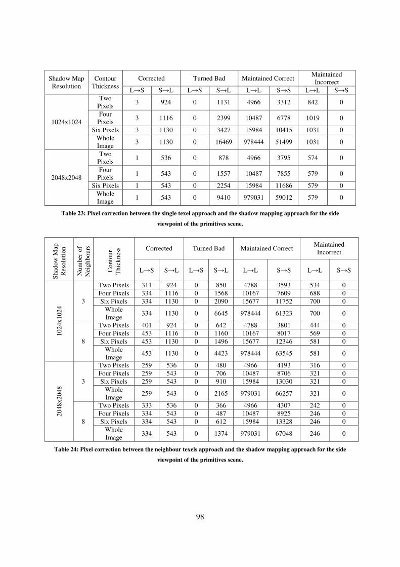
98
Shadow Map
Resolution
Contour
Thickness
Corrected Turned Bad Maintained Correct Maintained
Incorrect
L→S S→L L→S S→L L→L S→S L→L S→S
1024x1024
Two
Pixels 3 924 0 1131 4966 3312 842 0
Four
Pixels 3 1116 0 2399 10487 6778 1019 0
Six Pixels 3 1130 0 3427 15984 10415 1031 0
Whole
Image 3 1130 0 16469 978444 51499 1031 0
2048x2048
Two
Pixels 1 536 0 878 4966 3795 574 0
Four
Pixels 1 543 0 1557 10487 7855 579 0
Six Pixels 1 543 0 2254 15984 11686 579 0
Whole
Image 1 543 0 9410 979031 59012 579 0
Table 23: Pixel correction between the single texel approach and the shadow mapping approach for the side
viewpoint of the primitives scene.
Sh
ado
w M
ap
Res
olu
tio
n
Nu
mb
er o
f
Nei
gh
bo
urs
Co
nto
ur
Th
ick
nes
s Corrected Turned Bad Maintained Correct Maintained
Incorrect
L→S S→L L→S S→L L→L S→S L→L S→S
10
24x
102
4 3
Two Pixels 311 924 0 850 4788 3593 534 0
Four Pixels 334 1116 0 1568 10167 7609 688 0
Six Pixels 334 1130 0 2090 15677 11752 700 0
Whole
Image 334 1130 0 6645 978444 61323 700 0
8
Two Pixels 401 924 0 642 4788 3801 444 0
Four Pixels 453 1116 0 1160 10167 8017 569 0
Six Pixels 453 1130 0 1496 15677 12346 581 0
Whole
Image 453 1130 0 4423 978444 63545 581 0
20
48x
204
8 3
Two Pixels 259 536 0 480 4966 4193 316 0
Four Pixels 259 543 0 706 10487 8706 321 0
Six Pixels 259 543 0 910 15984 13030 321 0
Whole
Image 259 543 0 2165 979031 66257 321 0
8
Two Pixels 333 536 0 366 4966 4307 242 0
Four Pixels 334 543 0 487 10487 8925 246 0
Six Pixels 334 543 0 612 15984 13328 246 0
Whole
Image 334 543 0 1374 979031 67048 246 0
Table 24: Pixel correction between the neighbour texels approach and the shadow mapping approach for the side
viewpoint of the primitives scene.
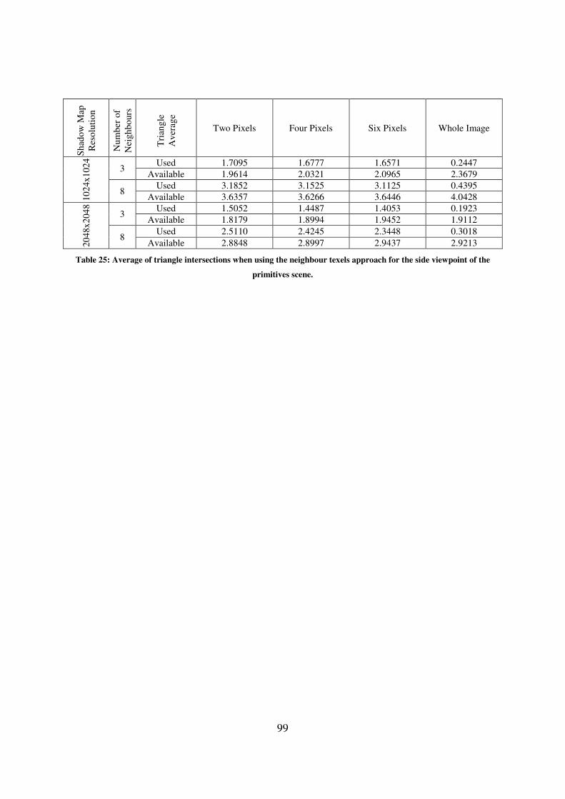
99
Sh
ado
w M
ap
Res
olu
tio
n
Nu
mb
er o
f
Nei
gh
bo
urs
Tri
ang
le
Av
erag
e
Two Pixels Four Pixels Six Pixels Whole Image
10
24x
102
4
3 Used 1.7095 1.6777 1.6571 0.2447
Available 1.9614 2.0321 2.0965 2.3679
8 Used 3.1852 3.1525 3.1125 0.4395
Available 3.6357 3.6266 3.6446 4.0428
20
48x
204
8
3 Used 1.5052 1.4487 1.4053 0.1923
Available 1.8179 1.8994 1.9452 1.9112
8 Used 2.5110 2.4245 2.3448 0.3018
Available 2.8848 2.8997 2.9437 2.9213
Table 25: Average of triangle intersections when using the neighbour texels approach for the side viewpoint of the
primitives scene.
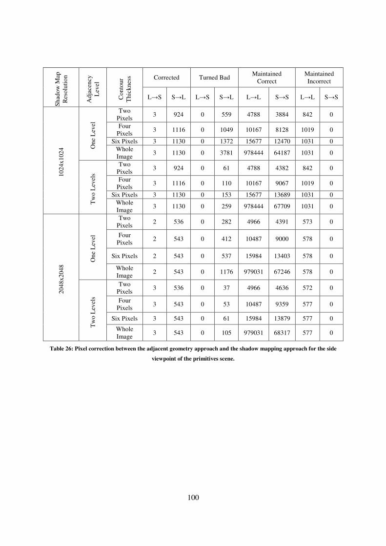
100
Sh
ado
w M
ap
Res
olu
tio
n
Ad
jace
ncy
Lev
el
Co
nto
ur
Th
ick
nes
s Corrected Turned Bad Maintained
Correct
Maintained
Incorrect
L→S S→L L→S S→L L→L S→S L→L S→S
10
24x
102
4 O
ne
Lev
el
Two
Pixels 3 924 0 559 4788 3884 842 0
Four
Pixels 3 1116 0 1049 10167 8128 1019 0
Six Pixels 3 1130 0 1372 15677 12470 1031 0
Whole
Image 3 1130 0 3781 978444 64187 1031 0
Tw
o L
evel
s
Two
Pixels 3 924 0 61 4788 4382 842 0
Four
Pixels 3 1116 0 110 10167 9067 1019 0
Six Pixels 3 1130 0 153 15677 13689 1031 0
Whole
Image 3 1130 0 259 978444 67709 1031 0
20
48x
204
8 O
ne
Lev
el
Two
Pixels 2 536 0 282 4966 4391 573 0
Four
Pixels 2 543 0 412 10487 9000 578 0
Six Pixels 2 543 0 537 15984 13403 578 0
Whole
Image 2 543 0 1176 979031 67246 578 0
Tw
o L
evel
s
Two
Pixels 3 536 0 37 4966 4636 572 0
Four
Pixels 3 543 0 53 10487 9359 577 0
Six Pixels 3 543 0 61 15984 13879 577 0
Whole
Image 3 543 0 105 979031 68317 577 0
Table 26: Pixel correction between the adjacent geometry approach and the shadow mapping approach for the side
viewpoint of the primitives scene.
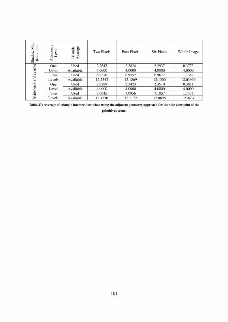
101
Sh
ado
w M
ap
Res
olu
tio
n
Ad
jace
ncy
Lev
el
Tri
ang
le
Av
erag
e
Two Pixels Four Pixels Six Pixels Whole Image
10
24x
102
4
One
Level
Used 2.2647 2.2824 2.2937 0.3773
Available 4.0000 4.0000 4.0000 4.0000
Two
Levels
Used 6.9370 6.9552 6.9672 1.1357
Available 12.2542 12.1869 12.1500 12.03966
20
48x
204
8
One
Level
Used 2.3289 2.3423 2.3510 0.3811
Available 4.0000 4.0000 4.0000 4.0000
Two
Levels
Used 7.0945 7.0956 7.1057 1.1476
Available 12.1850 12.1172 12.0896 12.0434
Table 27: Average of triangle intersections when using the adjacent geometry approach for the side viewpoint of the
primitives scene.
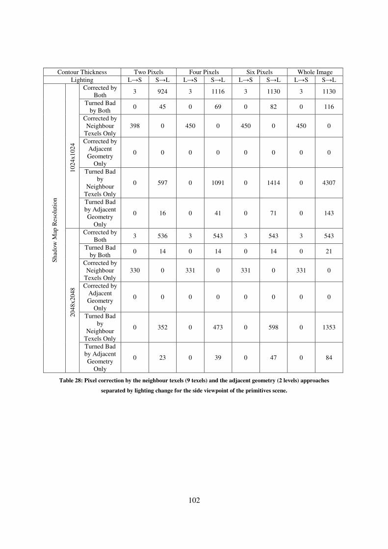
102
Contour Thickness Two Pixels Four Pixels Six Pixels Whole Image
Lighting L→S S→L L→S S→L L→S S→L L→S S→L
Sh
ado
w M
ap R
eso
luti
on
10
24x
102
4
Corrected by
Both 3 924 3 1116 3 1130 3 1130
Turned Bad
by Both 0 45 0 69 0 82 0 116
Corrected by
Neighbour
Texels Only
398 0 450 0 450 0 450 0
Corrected by
Adjacent
Geometry
Only
0 0 0 0 0 0 0 0
Turned Bad
by
Neighbour
Texels Only
0 597 0 1091 0 1414 0 4307
Turned Bad
by Adjacent
Geometry
Only
0 16 0 41 0 71 0 143
20
48x
204
8
Corrected by
Both 3 536 3 543 3 543 3 543
Turned Bad
by Both 0 14 0 14 0 14 0 21
Corrected by
Neighbour
Texels Only
330 0 331 0 331 0 331 0
Corrected by
Adjacent
Geometry
Only
0 0 0 0 0 0 0 0
Turned Bad
by
Neighbour
Texels Only
0 352 0 473 0 598 0 1353
Turned Bad
by Adjacent
Geometry
Only
0 23 0 39 0 47 0 84
Table 28: Pixel correction by the neighbour texels (9 texels) and the adjacent geometry (2 levels) approaches
separated by lighting change for the side viewpoint of the primitives scene.
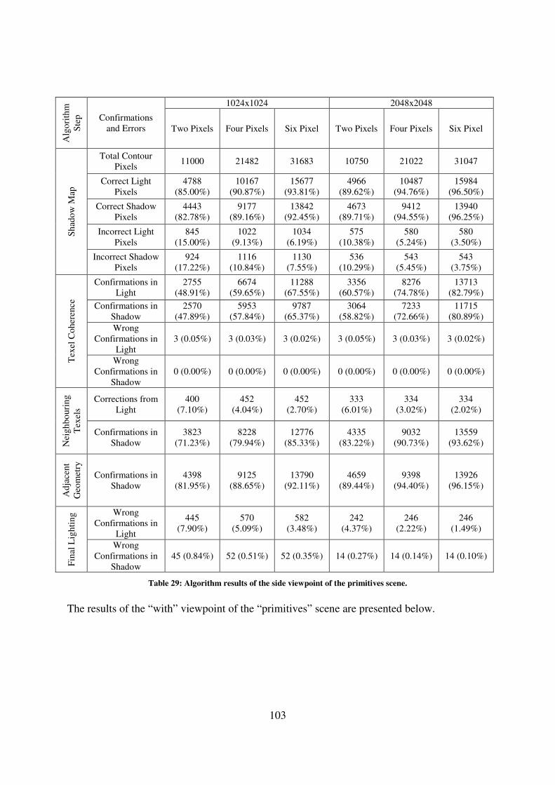
103
Alg
ori
thm
Ste
p
Confirmations
and Errors
1024x1024 2048x2048
Two Pixels Four Pixels Six Pixel Two Pixels Four Pixels Six Pixel
Sh
ado
w M
ap
Total Contour
Pixels 11000 21482 31683 10750 21022 31047
Correct Light
Pixels
4788
(85.00%)
10167
(90.87%)
15677
(93.81%)
4966
(89.62%)
10487
(94.76%)
15984
(96.50%)
Correct Shadow
Pixels
4443
(82.78%)
9177
(89.16%)
13842
(92.45%)
4673
(89.71%)
9412
(94.55%)
13940
(96.25%)
Incorrect Light
Pixels
845
(15.00%)
1022
(9.13%)
1034
(6.19%)
575
(10.38%)
580
(5.24%)
580
(3.50%)
Incorrect Shadow
Pixels
924
(17.22%)
1116
(10.84%)
1130
(7.55%)
536
(10.29%)
543
(5.45%)
543
(3.75%)
Tex
el C
oh
eren
ce
Confirmations in
Light
2755
(48.91%)
6674
(59.65%)
11288
(67.55%)
3356
(60.57%)
8276
(74.78%)
13713
(82.79%)
Confirmations in
Shadow
2570
(47.89%)
5953
(57.84%)
9787
(65.37%)
3064
(58.82%)
7233
(72.66%)
11715
(80.89%)
Wrong
Confirmations in
Light
3 (0.05%) 3 (0.03%) 3 (0.02%) 3 (0.05%) 3 (0.03%) 3 (0.02%)
Wrong
Confirmations in
Shadow
0 (0.00%) 0 (0.00%) 0 (0.00%) 0 (0.00%) 0 (0.00%) 0 (0.00%)
Nei
gh
bo
uri
ng
Tex
els
Corrections from
Light
400
(7.10%)
452
(4.04%)
452
(2.70%)
333
(6.01%)
334
(3.02%)
334
(2.02%)
Confirmations in
Shadow
3823
(71.23%)
8228
(79.94%)
12776
(85.33%)
4335
(83.22%)
9032
(90.73%)
13559
(93.62%)
Ad
jace
nt
Geo
met
ry
Confirmations in
Shadow
4398
(81.95%)
9125
(88.65%)
13790
(92.11%)
4659
(89.44%)
9398
(94.40%)
13926
(96.15%)
Fin
al L
igh
tin
g Wrong
Confirmations in
Light
445
(7.90%)
570
(5.09%)
582
(3.48%)
242
(4.37%)
246
(2.22%)
246
(1.49%)
Wrong
Confirmations in
Shadow
45 (0.84%) 52 (0.51%) 52 (0.35%) 14 (0.27%) 14 (0.14%) 14 (0.10%)
Table 29: Algorithm results of the side viewpoint of the primitives scene.
The results of the “with” viewpoint of the “primitives” scene are presented below.
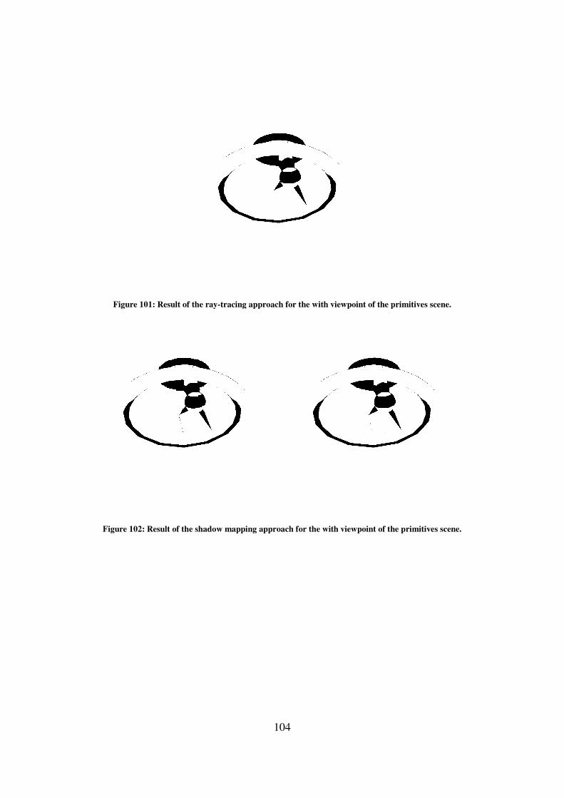
Figure 101: Result of the ray
Figure 102: Result of the shadow mapping approach for the
104
: Result of the ray-tracing approach for the with viewpoint of the primitives scene.
: Result of the shadow mapping approach for the with viewpoint of the primitives
tracing approach for the with viewpoint of the primitives scene.
primitives scene.
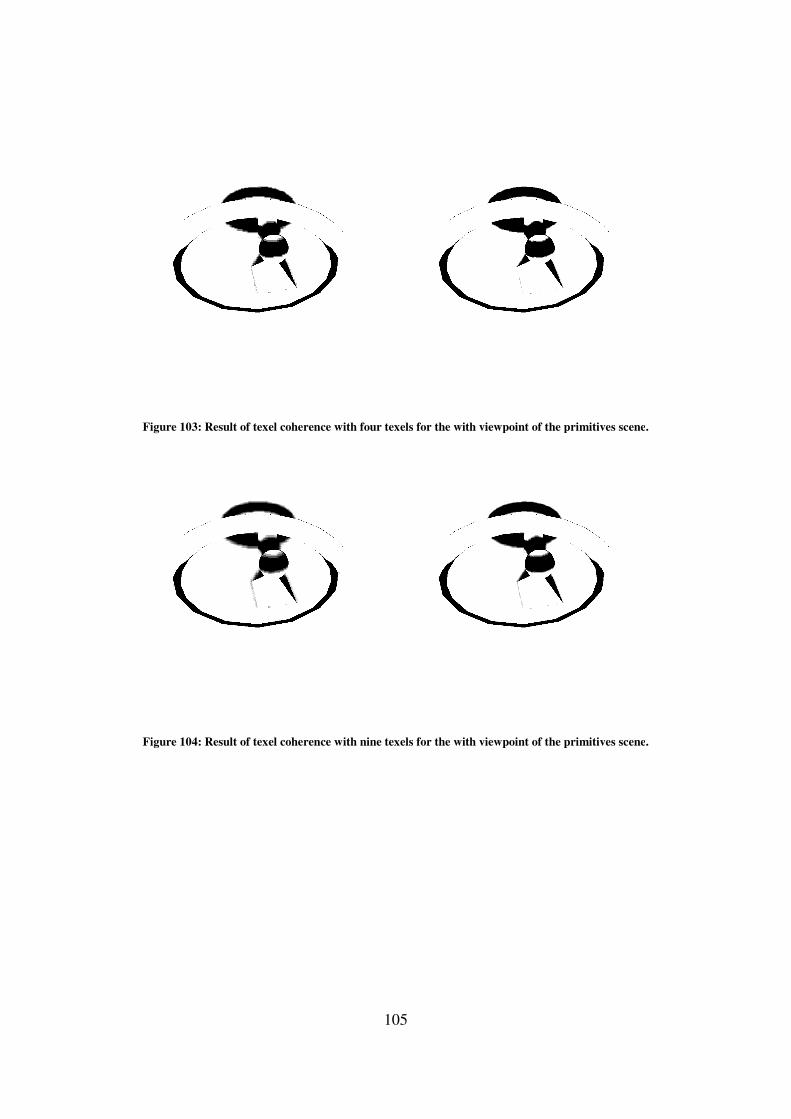
Figure 103: Result of texel coherence with four texels for
Figure 104: Result of texel coherence with nine texels for
105
: Result of texel coherence with four texels for the with viewpoint of the primitives scene
: Result of texel coherence with nine texels for the with viewpoint of the primitives scene
the with viewpoint of the primitives scene.
the with viewpoint of the primitives scene.
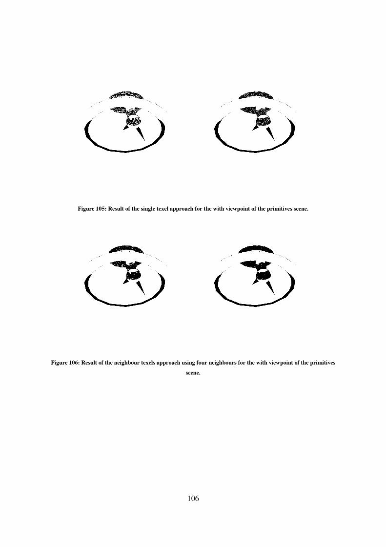
106
Figure 105: Result of the single texel approach for the with viewpoint of the primitives scene.
Figure 106: Result of the neighbour texels approach using four neighbours for the with viewpoint of the primitives
scene.
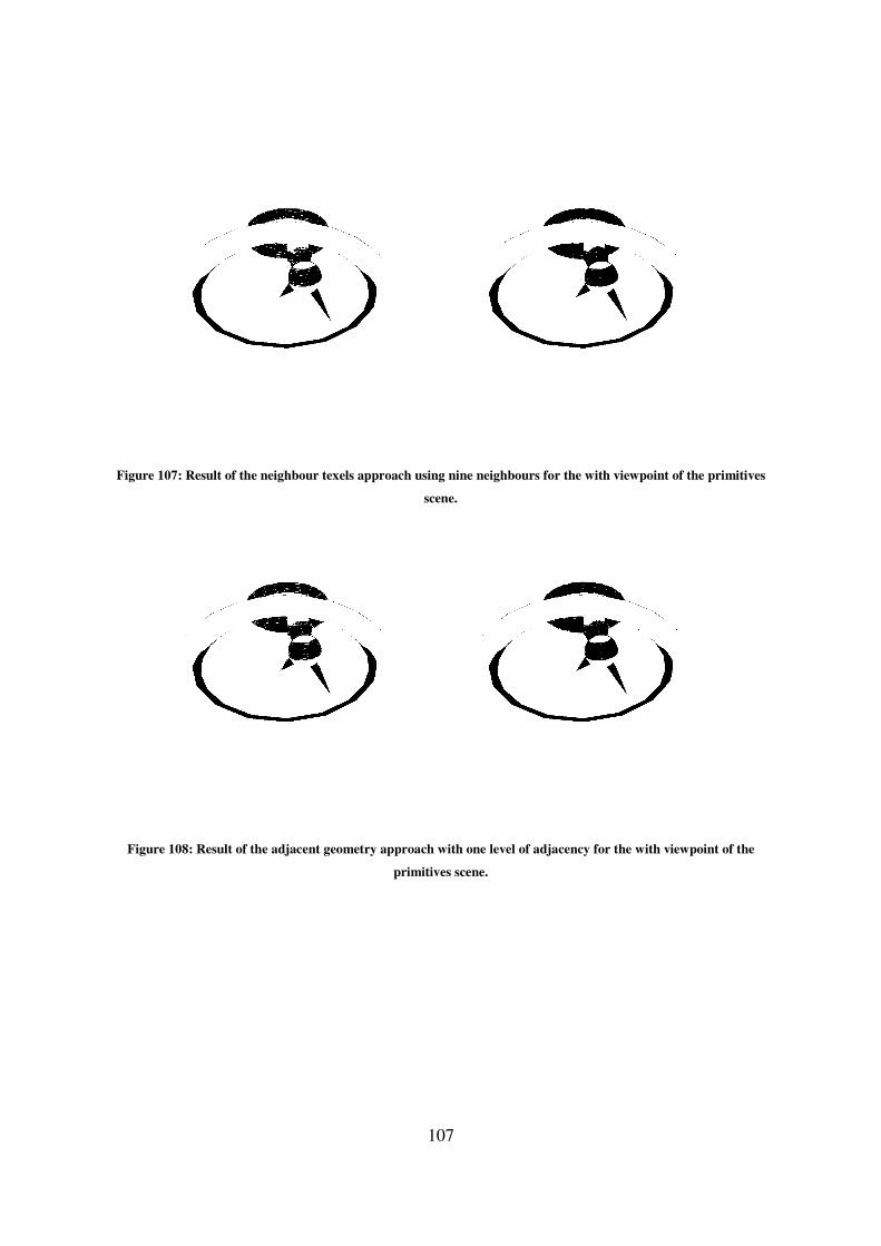
107
Figure 107: Result of the neighbour texels approach using nine neighbours for the with viewpoint of the primitives
scene.
Figure 108: Result of the adjacent geometry approach with one level of adjacency for the with viewpoint of the
primitives scene.
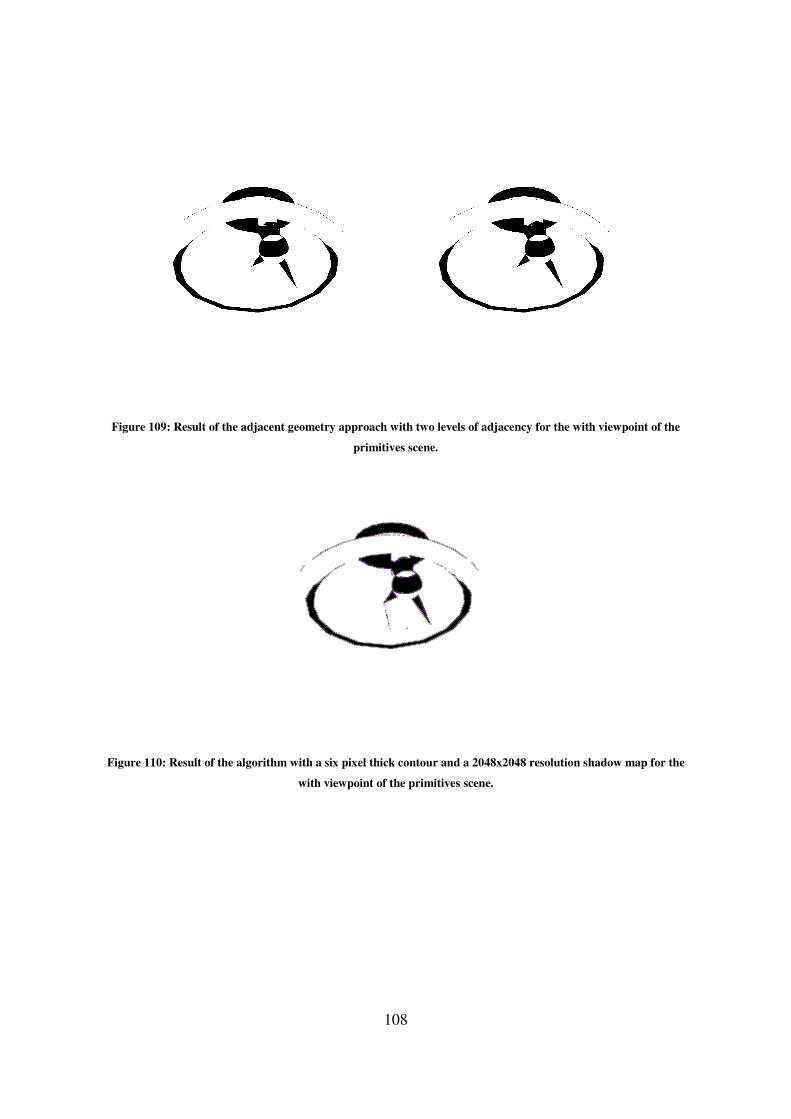
Figure 109: Result of the adjacent
Figure 110: Result of the algorithm with a six pixel thick contour and a 2048x2048 resolution shadow map for the
108
adjacent geometry approach with two levels of adjacency for the with viewpoint of the
primitives scene.
: Result of the algorithm with a six pixel thick contour and a 2048x2048 resolution shadow map for the
with viewpoint of the primitives scene.
the with viewpoint of the
: Result of the algorithm with a six pixel thick contour and a 2048x2048 resolution shadow map for the
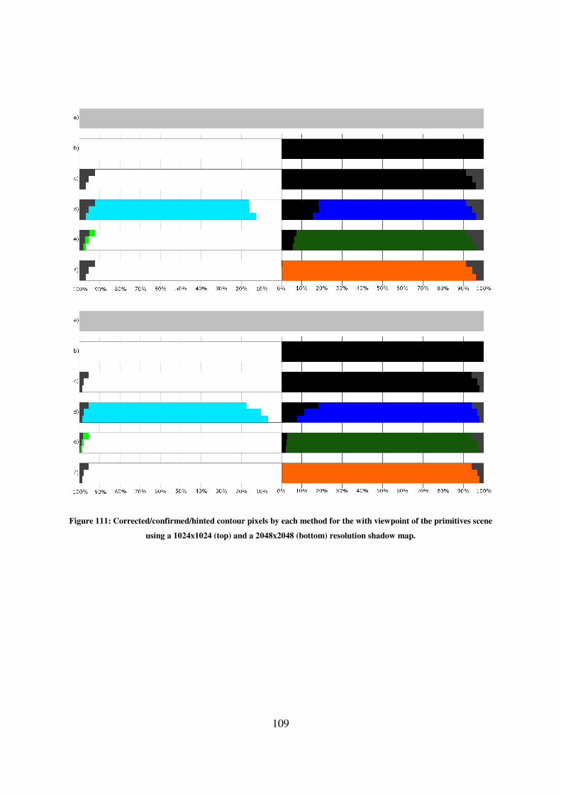
109
Figure 111: Corrected/confirmed/hinted contour pixels by each method for the with viewpoint of the primitives scene
using a 1024x1024 (top) and a 2048x2048 (bottom) resolution shadow map.
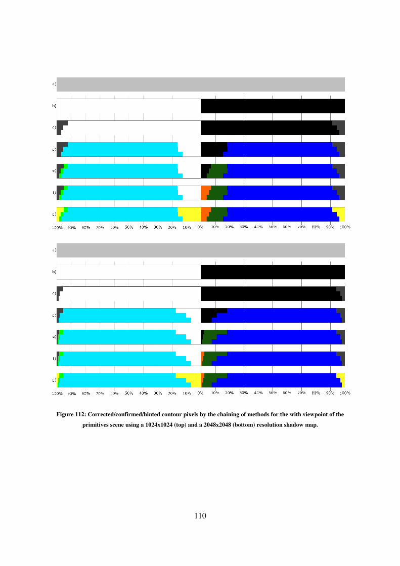
110
Figure 112: Corrected/confirmed/hinted contour pixels by the chaining of methods for the with viewpoint of the
primitives scene using a 1024x1024 (top) and a 2048x2048 (bottom) resolution shadow map.

111
Shadow Map
Resolution Approach
Contour Thickness
Two Pixels Four Pixels Six Pixels Whole Image
1024x1024
Pixels in
Contour 12244 24077 35874 1048576
Shadow Map 1004 (8.20%) 1211 (5.03%) 1221 (3.40%) 1221 (0.12%)
Single Texel 1310 (10.7%) 2087 (8.67%) 2759 (7.69%) 9815 (0.94%)
Neighbour
Texels (4
Neighbours)
892 (7.29%) 1296 (5.38%) 1563 (4.36%) 3583 (0.34%)
Neighbour
Texels (9
Neighbours)
729 (5.95%) 1023 (4.25%) 1211 (3.38%) 2517 (0.24%)
Adjacent
Geometry (One
Level)
818 (6.68%) 1069 (4.44%) 1213 (3.38%) 2166 (0.21%)
Adjacent
Geometry
(Two Level)
533 (4.35%) 651 (2.70%) 662 (1.85%) 695 (0.07%)
2048x2048
Pixels in
Contour 12249 24119 35959 1048576
Shadow Map 620 (5.06%) 626 (2.60%) 628 (1.75%) 628 (0.06%)
Single Texel 725 (5.92%) 1210 (5.02%) 1677 (4.66%) 5208 (0.50%)
Neighbour
Texels (4
Neighbours)
367 (3.00%) 523 (2.17%) 649 (1.80%) 1105 (0.11%)
Neighbour
Texels (9
Neighbours)
279 (2.28%) 379 (1.57%) 449 (1.25%) 692 (0.07%)
Adjacent
Geometry (One
Level)
381 (3.11%) 445 (1.85%) 525 (1.46%) 728 (0.07%)
Adjacent
Geometry
(Two Level)
293 (2.39%) 300 (1.24%) 302 (0.84%) 314 (0.03%)
Table 30: Difference between the approaches that use ray-tracing and the actual ray-tracer for the with viewpoint of
the primitives scene.
Shadow Map Resolution Contour Thickness
Two Pixels Four Pixels Six Pixels
1024x1024 1004 of 1221 (82.23%) 1211 of 1221 (99.18%) 1221 of 1221 (100.00%)
2048x2048 620 of 628 (98.73%) 626 of 628 (99.68%) 628 of 628 (100.00%)
Table 31: Wrongly defined pixels in the shadow mapping result which are inside the contour in the with viewpoint of
the primitives scene.

112
Shadow Map Resolution Contour Thickness Pixel Shading
Light Shadow
1024x1024
Two Pixels 518 of 6752 486 of 5492
Four Pixels 634 of 13807 577 of 10270
Six Pixels 642 of 21006 579 of 14868
Whole Image 642 of 1001569 579 of 47007
2048x2048
Two Pixels 292 of 6771 328 of 5478
Four Pixels 296 of 13854 330 of 10265
Six Pixels 298 of 21081 330 of 14878
Whole Image 298 of 1001474 330 of 47102
Table 32: Pixels that the shadow map defines wrongly in the with viewpoint of the primitives scene, separated in
pixels defined in light and in shadow, compared to the total amount of pixels lighted in the same way.
Shadow
Map
Resolution
Contour
Thickness
Texel Coherence
Light Shadow
Confirmed Incorrectly
Confirmed Undecided Confirmed
Incorrectly
Confirmed Undecided
1024x1024
Two Pixels 5137
(76.08%) 3 (0.04%)
1615
(23.92%)
3995
(72.74%) 0 (0.00%)
1497
(27.26%)
Four Pixels 10965
(79.42%) 6 (0.04%)
2842
(20.58%)
7773
(75.69%) 0 (0.00%)
2497
(24.31%)
Six Pixels 17697
(84.25%) 8 (0.04%)
3309
(15.75%)
12007
(80.76%) 0 (0.00%)
2861
(19.24%)
Whole
Image
998128
(99.66%) 8 (0.00%)
3441
(0.34%)
44126
(93.87%) 0 (0.00%)
2881
(6.13%)
2048x2048
Two Pixels 5294
(78.19%) 2 (0.03%)
1477
(21.81%)
4143
(75.63%) 0 (0.00%)
1335
(24.37%)
Four Pixels 12124
(87.51%) 4 (0.03%)
1730
(12.49%)
8800
(85.73%) 0 (0.00%)
1465
(14.27%)
Six Pixels 19331
(91.70%) 6 (0.03%)
1750
(8.30%)
13413
(90.15%) 0 (0.00%)
1465
(9.85%)
Whole
Image
999672
(99.82%) 6 (0.00%)
1802
(0.18%)
45637
(96.89%) 0 (0.00%)
1465
(3.11%)
Table 33: Pixel confirmation when using texel coherence with four texels for the with viewpoint of the primitives
scene.
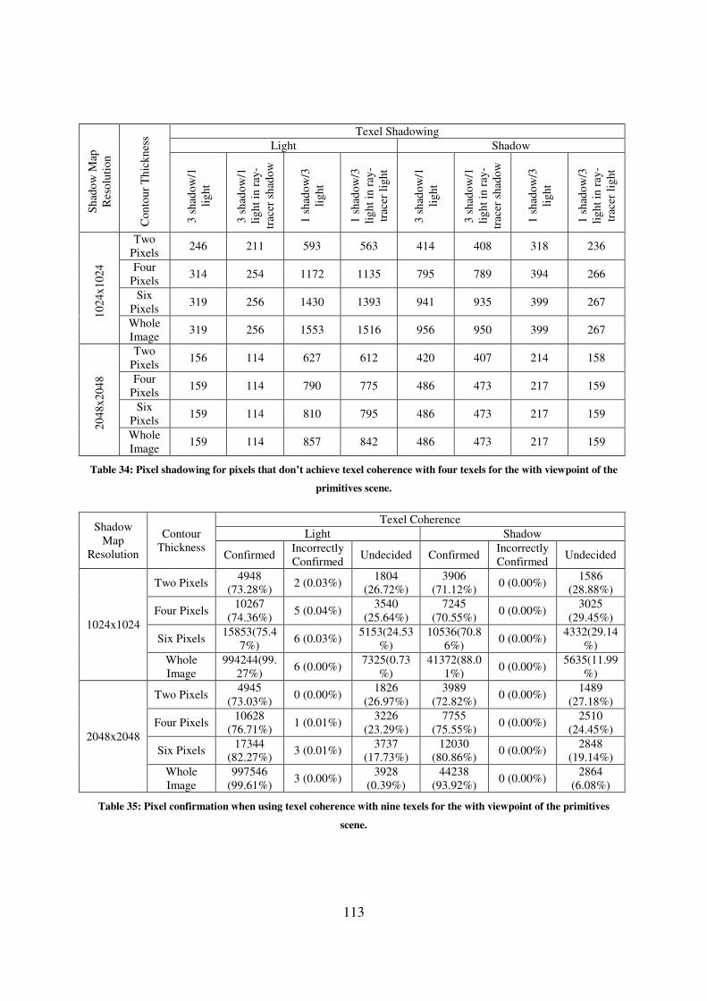
113
Sh
ado
w M
ap
Res
olu
tio
n
Co
nto
ur
Th
ick
nes
s Texel Shadowing
Light Shadow
3 s
had
ow
/1
lig
ht
3 s
had
ow
/1
lig
ht
in r
ay-
trac
er s
had
ow
1 s
had
ow
/3
lig
ht
1 s
had
ow
/3
lig
ht
in r
ay-
trac
er l
igh
t
3 s
had
ow
/1
lig
ht
3 s
had
ow
/1
lig
ht
in r
ay-
trac
er s
had
ow
1 s
had
ow
/3
lig
ht
1 s
had
ow
/3
lig
ht
in r
ay-
trac
er l
igh
t
10
24x
102
4
Two
Pixels 246 211 593 563 414 408 318 236
Four
Pixels 314 254 1172 1135 795 789 394 266
Six
Pixels 319 256 1430 1393 941 935 399 267
Whole
Image 319 256 1553 1516 956 950 399 267
20
48x
204
8
Two
Pixels 156 114 627 612 420 407 214 158
Four
Pixels 159 114 790 775 486 473 217 159
Six
Pixels 159 114 810 795 486 473 217 159
Whole
Image 159 114 857 842 486 473 217 159
Table 34: Pixel shadowing for pixels that don’t achieve texel coherence with four texels for the with viewpoint of the
primitives scene.
Shadow
Map
Resolution
Contour
Thickness
Texel Coherence
Light Shadow
Confirmed Incorrectly
Confirmed Undecided Confirmed
Incorrectly
Confirmed Undecided
1024x1024
Two Pixels 4948
(73.28%) 2 (0.03%)
1804
(26.72%)
3906
(71.12%) 0 (0.00%)
1586
(28.88%)
Four Pixels 10267
(74.36%) 5 (0.04%)
3540
(25.64%)
7245
(70.55%) 0 (0.00%)
3025
(29.45%)
Six Pixels 15853(75.4
7%) 6 (0.03%)
5153(24.53
%)
10536(70.8
6%) 0 (0.00%)
4332(29.14
%)
Whole
Image
994244(99.
27%) 6 (0.00%)
7325(0.73
%)
41372(88.0
1%) 0 (0.00%)
5635(11.99
%)
2048x2048
Two Pixels 4945
(73.03%) 0 (0.00%)
1826
(26.97%)
3989
(72.82%) 0 (0.00%)
1489
(27.18%)
Four Pixels 10628
(76.71%) 1 (0.01%)
3226
(23.29%)
7755
(75.55%) 0 (0.00%)
2510
(24.45%)
Six Pixels 17344
(82.27%) 3 (0.01%)
3737
(17.73%)
12030
(80.86%) 0 (0.00%)
2848
(19.14%)
Whole
Image
997546
(99.61%) 3 (0.00%)
3928
(0.39%)
44238
(93.92%) 0 (0.00%)
2864
(6.08%)
Table 35: Pixel confirmation when using texel coherence with nine texels for the with viewpoint of the primitives
scene.

114
Sh
ado
w M
ap
Lig
hti
ng
Tex
el
Sh
ado
win
g Shadow Map
1024x1024 2048x2048
Two
Pixels
Four
Pixels
Six
Pixels
Whole
Image
Two
Pixels
Four
Pixels
Six
Pixels
Whole
Image
Lig
ht
8 S-1 L 0 0 0 0 0 0 0 0
8 S-1 L in
RT Shadow 0 0 0 0 0 0 0 0
7 S-2 L 0 0 0 0 0 0 0 0
7 S-2 L in
RT Shadow 0 0 0 0 0 0 0 0
6 S-3 L 0 0 0 0 0 0 0 0
6 S-3 L in
RT Shadow 0 0 0 0 0 0 0 0
5 S-4 L 21 35 42 44 7 10 10 10
5 S-4 L in
RT Shadow 12 12 12 12 4 4 4 4
4 S-5 L 363 594 711 756 329 413 418 418
4 S-5 L in
RT Light 147 323 439 484 190 273 278 278
3 S-6 L 762 1466 2088 2716 719 1209 1344 1358
3 S-6 L in
RT Light 479 1125 1742 2370 575 1064 1199 1213
2 S-7 L 374 708 1007 1404 329 552 633 700
2 S-7 L in
RT Light 371 705 1004 1401 328 551 632 699
1 S-8 L 284 737 1305 2405 442 1042 1332 1442
1 S-8 L in
RT Light 282 735 1302 2402 438 1037 1327 1437
Sh
ado
w
8 S-1 L 111 382 753 1235 174 484 607 617
8 S-1 L in
RT Shadow 111 382 753 1235 172 482 605 615
7 S-2 L 248 475 689 892 230 387 437 441
7 S-2 L in
RT Shadow 244 471 685 888 224 381 431 435
6 S-3 L 751 1428 2013 2573 693 1148 1308 1310
6 S-3 L in
RT Shadow 570 1214 1799 2359 584 1039 1199 1201
5 S-4 L 394 651 788 846 338 436 441 441
5 S-4 L in
RT Shadow 175 381 516 574 180 277 282 282
4 S-5 L 36 41 41 41 19 19 19 19
4 S-5 L in
RT Light 36 41 41 41 19 19 19 19
3 S-6 L 38 40 40 40 19 19 19 19
3 S-6 L in
RT Light 38 40 40 40 19 19 19 19
2 S-7 L 8 8 8 8 6 6 6 6
2 S-7 L in
RT Light 8 8 8 8 6 6 6 6
1 S-8 L 0 0 0 0 10 11 11 11
1 S-8 L in
RT Light 0 0 0 0 9 10 10 10
Table 36: Pixel shadowing for pixels that don’t achieve texel coherence with nine texels for the with viewpoint of the
primitives scene.
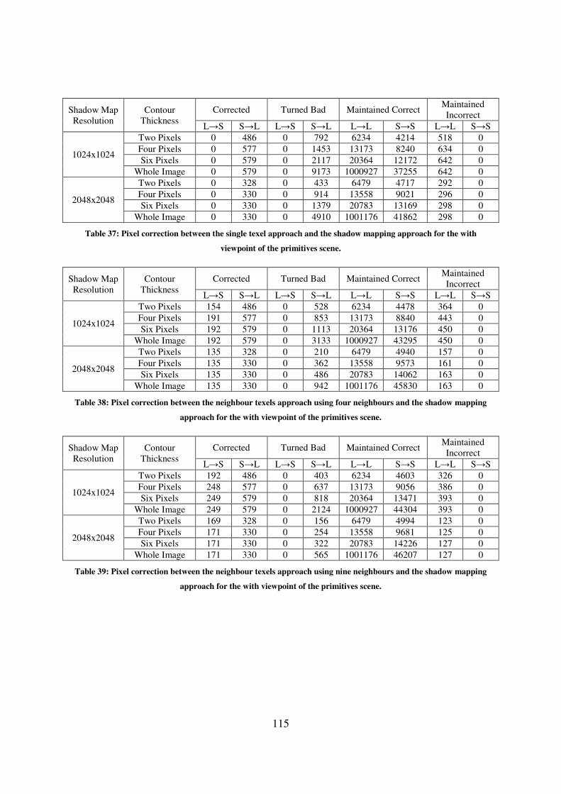
115
Shadow Map
Resolution
Contour
Thickness
Corrected Turned Bad Maintained Correct Maintained
Incorrect
L→S S→L L→S S→L L→L S→S L→L S→S
1024x1024
Two Pixels 0 486 0 792 6234 4214 518 0
Four Pixels 0 577 0 1453 13173 8240 634 0
Six Pixels 0 579 0 2117 20364 12172 642 0
Whole Image 0 579 0 9173 1000927 37255 642 0
2048x2048
Two Pixels 0 328 0 433 6479 4717 292 0
Four Pixels 0 330 0 914 13558 9021 296 0
Six Pixels 0 330 0 1379 20783 13169 298 0
Whole Image 0 330 0 4910 1001176 41862 298 0
Table 37: Pixel correction between the single texel approach and the shadow mapping approach for the with
viewpoint of the primitives scene.
Shadow Map
Resolution
Contour
Thickness
Corrected Turned Bad Maintained Correct Maintained
Incorrect
L→S S→L L→S S→L L→L S→S L→L S→S
1024x1024
Two Pixels 154 486 0 528 6234 4478 364 0
Four Pixels 191 577 0 853 13173 8840 443 0
Six Pixels 192 579 0 1113 20364 13176 450 0
Whole Image 192 579 0 3133 1000927 43295 450 0
2048x2048
Two Pixels 135 328 0 210 6479 4940 157 0
Four Pixels 135 330 0 362 13558 9573 161 0
Six Pixels 135 330 0 486 20783 14062 163 0
Whole Image 135 330 0 942 1001176 45830 163 0
Table 38: Pixel correction between the neighbour texels approach using four neighbours and the shadow mapping
approach for the with viewpoint of the primitives scene.
Shadow Map
Resolution
Contour
Thickness
Corrected Turned Bad Maintained Correct Maintained
Incorrect
L→S S→L L→S S→L L→L S→S L→L S→S
1024x1024
Two Pixels 192 486 0 403 6234 4603 326 0
Four Pixels 248 577 0 637 13173 9056 386 0
Six Pixels 249 579 0 818 20364 13471 393 0
Whole Image 249 579 0 2124 1000927 44304 393 0
2048x2048
Two Pixels 169 328 0 156 6479 4994 123 0
Four Pixels 171 330 0 254 13558 9681 125 0
Six Pixels 171 330 0 322 20783 14226 127 0
Whole Image 171 330 0 565 1001176 46207 127 0
Table 39: Pixel correction between the neighbour texels approach using nine neighbours and the shadow mapping
approach for the with viewpoint of the primitives scene.
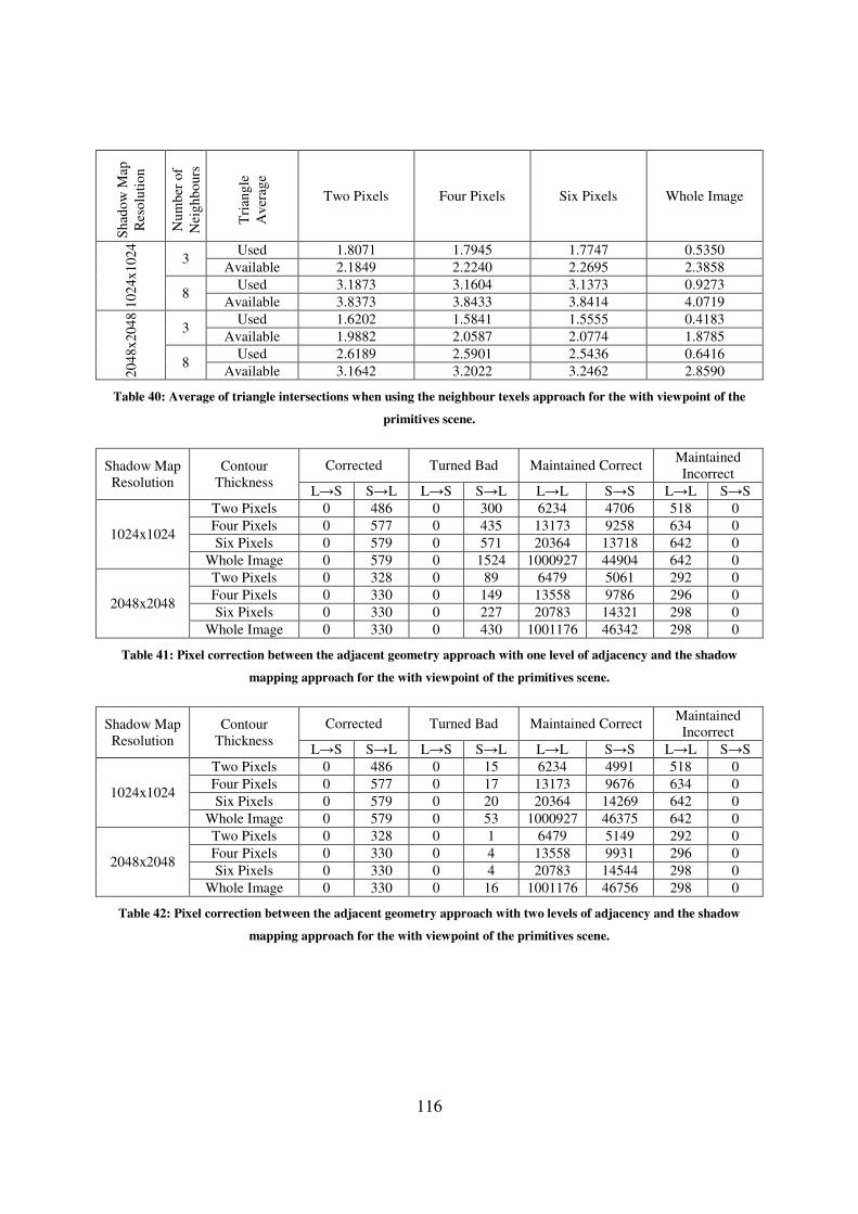
116
Sh
ado
w M
ap
Res
olu
tio
n
Nu
mb
er o
f
Nei
gh
bo
urs
Tri
ang
le
Av
erag
e
Two Pixels Four Pixels Six Pixels Whole Image
10
24x
102
4
3 Used 1.8071 1.7945 1.7747 0.5350
Available 2.1849 2.2240 2.2695 2.3858
8 Used 3.1873 3.1604 3.1373 0.9273
Available 3.8373 3.8433 3.8414 4.0719
20
48x
204
8
3 Used 1.6202 1.5841 1.5555 0.4183
Available 1.9882 2.0587 2.0774 1.8785
8 Used 2.6189 2.5901 2.5436 0.6416
Available 3.1642 3.2022 3.2462 2.8590
Table 40: Average of triangle intersections when using the neighbour texels approach for the with viewpoint of the
primitives scene.
Shadow Map
Resolution
Contour
Thickness
Corrected Turned Bad Maintained Correct Maintained
Incorrect
L→S S→L L→S S→L L→L S→S L→L S→S
1024x1024
Two Pixels 0 486 0 300 6234 4706 518 0
Four Pixels 0 577 0 435 13173 9258 634 0
Six Pixels 0 579 0 571 20364 13718 642 0
Whole Image 0 579 0 1524 1000927 44904 642 0
2048x2048
Two Pixels 0 328 0 89 6479 5061 292 0
Four Pixels 0 330 0 149 13558 9786 296 0
Six Pixels 0 330 0 227 20783 14321 298 0
Whole Image 0 330 0 430 1001176 46342 298 0
Table 41: Pixel correction between the adjacent geometry approach with one level of adjacency and the shadow
mapping approach for the with viewpoint of the primitives scene.
Shadow Map
Resolution
Contour
Thickness
Corrected Turned Bad Maintained Correct Maintained
Incorrect
L→S S→L L→S S→L L→L S→S L→L S→S
1024x1024
Two Pixels 0 486 0 15 6234 4991 518 0
Four Pixels 0 577 0 17 13173 9676 634 0
Six Pixels 0 579 0 20 20364 14269 642 0
Whole Image 0 579 0 53 1000927 46375 642 0
2048x2048
Two Pixels 0 328 0 1 6479 5149 292 0
Four Pixels 0 330 0 4 13558 9931 296 0
Six Pixels 0 330 0 4 20783 14544 298 0
Whole Image 0 330 0 16 1001176 46756 298 0
Table 42: Pixel correction between the adjacent geometry approach with two levels of adjacency and the shadow
mapping approach for the with viewpoint of the primitives scene.

117
Sh
ado
w M
ap
Res
olu
tio
n
Ad
jace
ncy
Lev
el
Tri
ang
le
Av
erag
e
Two Pixels Four Pixels Six Pixels Whole Image
10
24x
102
4
One
Level
Used 2.4802 2.5010 2.5125 0.8570
Available 4.0000 4.0000 4.0000 4.0000
Two
Levels
Used 7.5215 7.1057 7.6283 2.6583
Available 12.1303 12.1380 12.1448 12.4070
20
48x
204
8
One
Level
Used 2.5974 2.6077 2.6164 0.8670
Available 4.0000 4.0000 4.0000 4.0000
Two
Levels
Used 7.9256 7.1057 7.9950 2.6924
Available 12.2053 12.2097 12.2229 12.4218
Table 43: Average of triangle intersections when using the adjacent geometry approach for the with viewpoint of the
primitives scene.

118
Contour Thickness Two Pixels Four Pixels Six Pixels Whole Image
Lighting L→S S→L L→S S→L L→S S→L L→S S→L
Sh
ado
w M
ap R
eso
luti
on
10
24x
102
4
Corrected by
Both 0 486 0 577 0 579 0 579
Turned Bad
by Both 0 14 0 16 0 18 0 33
Corrected by
Neighbour
Texels Only
192 0 248 0 249 0 249 0
Corrected by
Adjacent
Geometry
Only
0 0 0 0 0 0 0 0
Turned Bad
by
Neighbour
Texels Only
0 389 0 621 0 800 0 2091
Turned Bad
by Adjacent
Geometry
Only
0 1 0 1 0 2 0 20
20
48x
204
8
Corrected by
Both 0 328 0 330 0 330 0 330
Turned Bad
by Both 0 1 0 2 0 2 0 3
Corrected by
Neighbour
Texels Only
169 0 171 0 171 0 171 0
Corrected by
Adjacent
Geometry
Only
0 0 0 0 0 0 0 0
Turned Bad
by
Neighbour
Texels Only
0 155 0 252 0 320 0 562
Turned Bad
by Adjacent
Geometry
Only
0 0 0 2 0 2 0 13
Table 44: Pixel correction by the neighbour texels (9 texels) and the adjacent geometry (2 levels) approaches
separated by lighting change for the with viewpoint of the primitives scene.
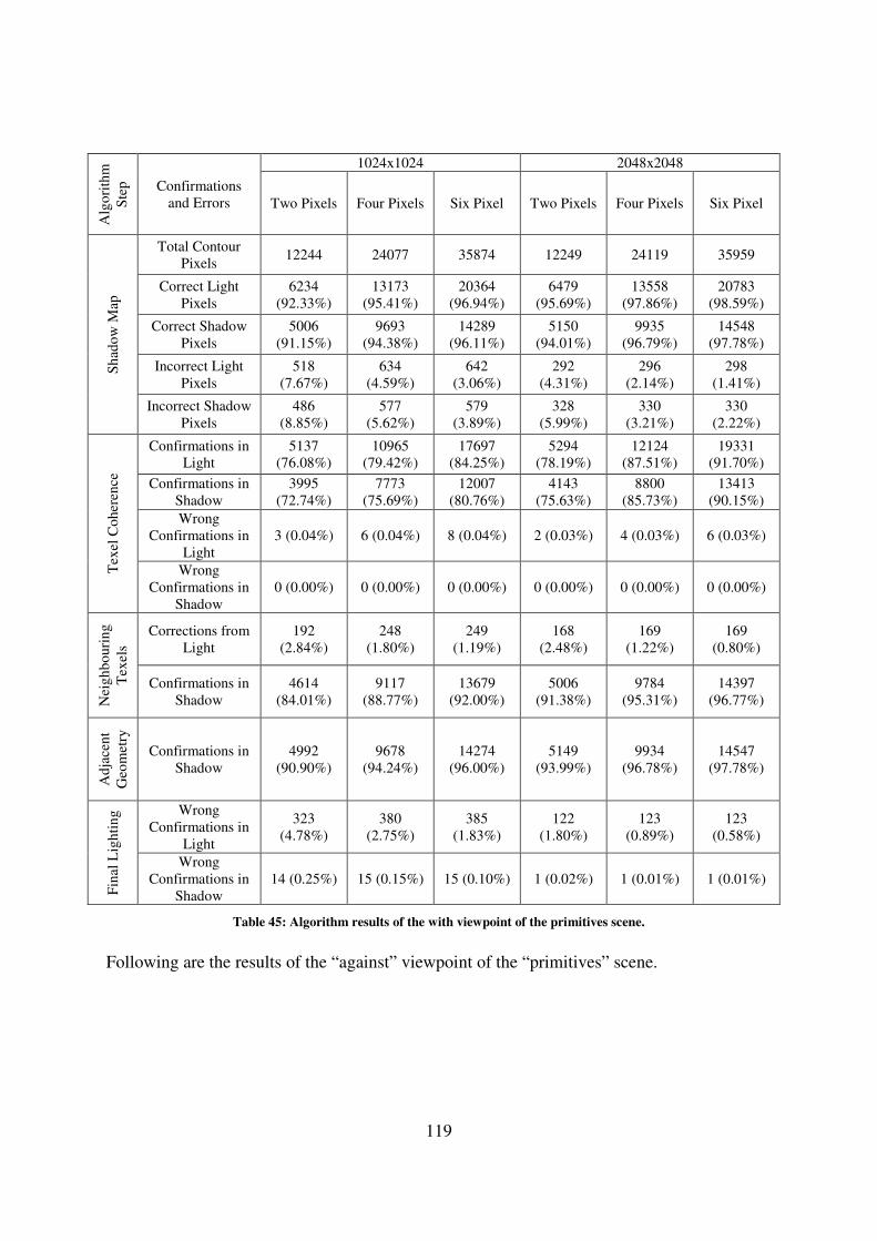
119
Alg
ori
thm
Ste
p
Confirmations
and Errors
1024x1024 2048x2048
Two Pixels Four Pixels Six Pixel Two Pixels Four Pixels Six Pixel
Sh
ado
w M
ap
Total Contour
Pixels 12244 24077 35874 12249 24119 35959
Correct Light
Pixels
6234
(92.33%)
13173
(95.41%)
20364
(96.94%)
6479
(95.69%)
13558
(97.86%)
20783
(98.59%)
Correct Shadow
Pixels
5006
(91.15%)
9693
(94.38%)
14289
(96.11%)
5150
(94.01%)
9935
(96.79%)
14548
(97.78%)
Incorrect Light
Pixels
518
(7.67%)
634
(4.59%)
642
(3.06%)
292
(4.31%)
296
(2.14%)
298
(1.41%)
Incorrect Shadow
Pixels
486
(8.85%)
577
(5.62%)
579
(3.89%)
328
(5.99%)
330
(3.21%)
330
(2.22%)
Tex
el C
oh
eren
ce
Confirmations in
Light
5137
(76.08%)
10965
(79.42%)
17697
(84.25%)
5294
(78.19%)
12124
(87.51%)
19331
(91.70%)
Confirmations in
Shadow
3995
(72.74%)
7773
(75.69%)
12007
(80.76%)
4143
(75.63%)
8800
(85.73%)
13413
(90.15%)
Wrong
Confirmations in
Light
3 (0.04%) 6 (0.04%) 8 (0.04%) 2 (0.03%) 4 (0.03%) 6 (0.03%)
Wrong
Confirmations in
Shadow
0 (0.00%) 0 (0.00%) 0 (0.00%) 0 (0.00%) 0 (0.00%) 0 (0.00%)
Nei
gh
bo
uri
ng
Tex
els
Corrections from
Light
192
(2.84%)
248
(1.80%)
249
(1.19%)
168
(2.48%)
169
(1.22%)
169
(0.80%)
Confirmations in
Shadow
4614
(84.01%)
9117
(88.77%)
13679
(92.00%)
5006
(91.38%)
9784
(95.31%)
14397
(96.77%)
Ad
jace
nt
Geo
met
ry
Confirmations in
Shadow
4992
(90.90%)
9678
(94.24%)
14274
(96.00%)
5149
(93.99%)
9934
(96.78%)
14547
(97.78%)
Fin
al L
igh
tin
g Wrong
Confirmations in
Light
323
(4.78%)
380
(2.75%)
385
(1.83%)
122
(1.80%)
123
(0.89%)
123
(0.58%)
Wrong
Confirmations in
Shadow
14 (0.25%) 15 (0.15%) 15 (0.10%) 1 (0.02%) 1 (0.01%) 1 (0.01%)
Table 45: Algorithm results of the with viewpoint of the primitives scene.
Following are the results of the “against” viewpoint of the “primitives” scene.
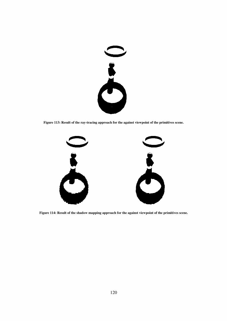
Figure 113: Result of the ray
Figure 114: Result of the shadow mapping approach for the
120
: Result of the ray-tracing approach for the against viewpoint of the primitives scene.
he shadow mapping approach for the against viewpoint of the primitives
tracing approach for the against viewpoint of the primitives scene.
primitives scene.
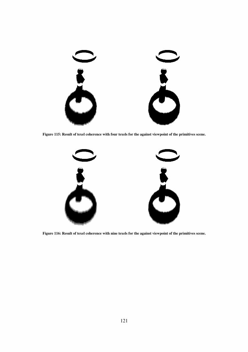
Figure 115: Result of texel coherence with four texels for
Figure 116: Result of texel coherence with nine texels for
121
: Result of texel coherence with four texels for the against viewpoint of the primitives scene
: Result of texel coherence with nine texels for the against viewpoint of the primitives scene
the against viewpoint of the primitives scene.
the against viewpoint of the primitives scene.
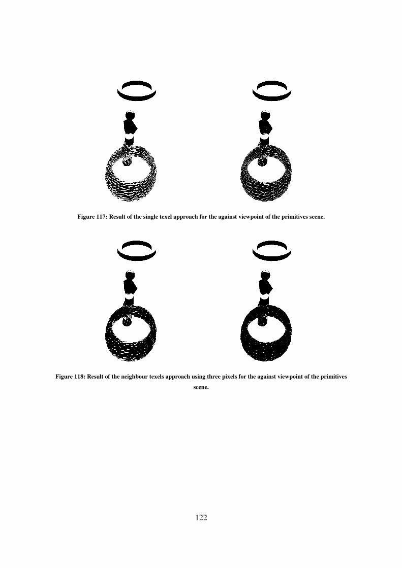
122
Figure 117: Result of the single texel approach for the against viewpoint of the primitives scene.
Figure 118: Result of the neighbour texels approach using three pixels for the against viewpoint of the primitives
scene.
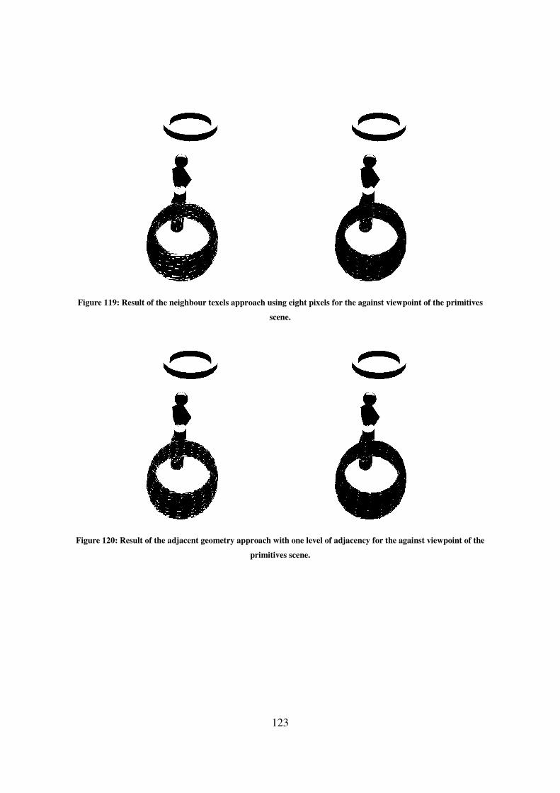
123
Figure 119: Result of the neighbour texels approach using eight pixels for the against viewpoint of the primitives
scene.
Figure 120: Result of the adjacent geometry approach with one level of adjacency for the against viewpoint of the
primitives scene.
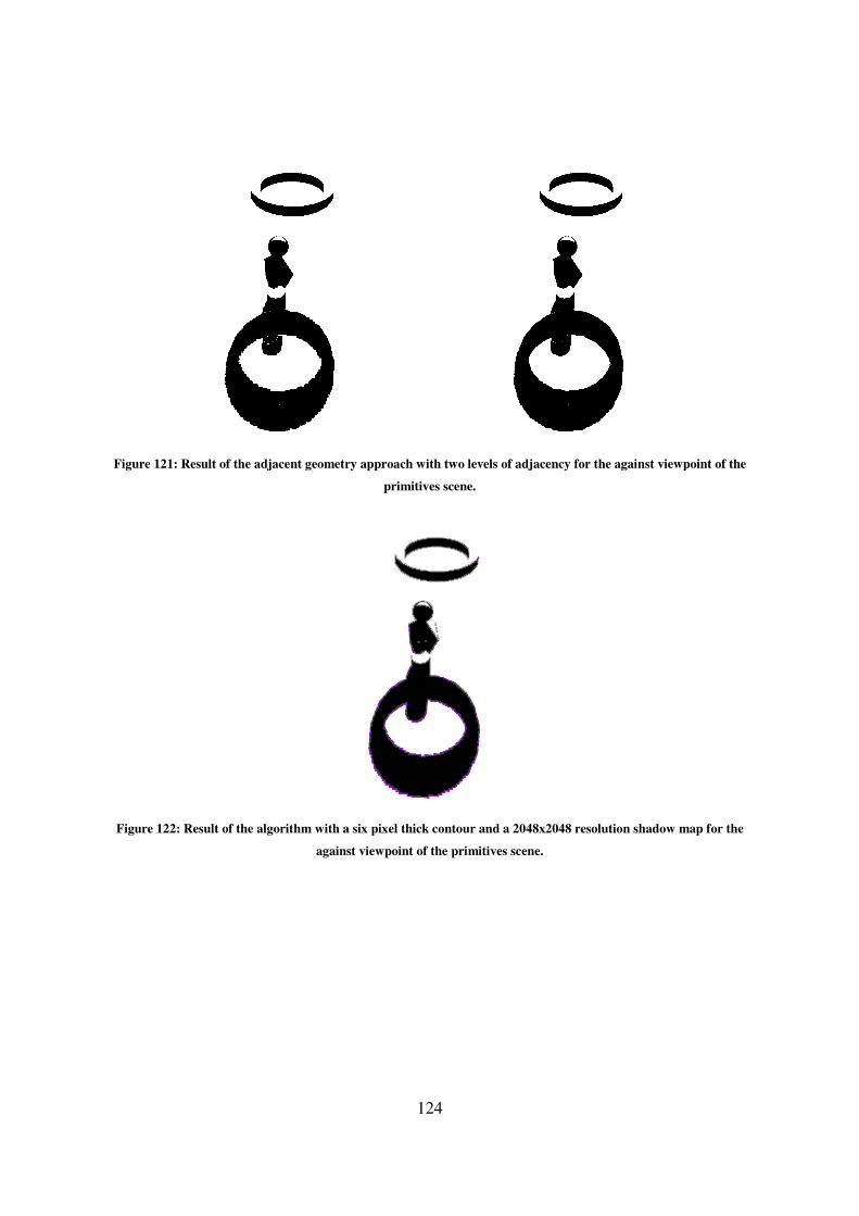
Figure 121: Result of the adjacent geometry
Figure 122: Result of the algorithm with a six pixel thick contour and a 2048x2048 resolution shadow map for the
124
adjacent geometry approach with two levels of adjacency for the against viewpoint of the
primitives scene.
: Result of the algorithm with a six pixel thick contour and a 2048x2048 resolution shadow map for the
against viewpoint of the primitives scene.
the against viewpoint of the
: Result of the algorithm with a six pixel thick contour and a 2048x2048 resolution shadow map for the
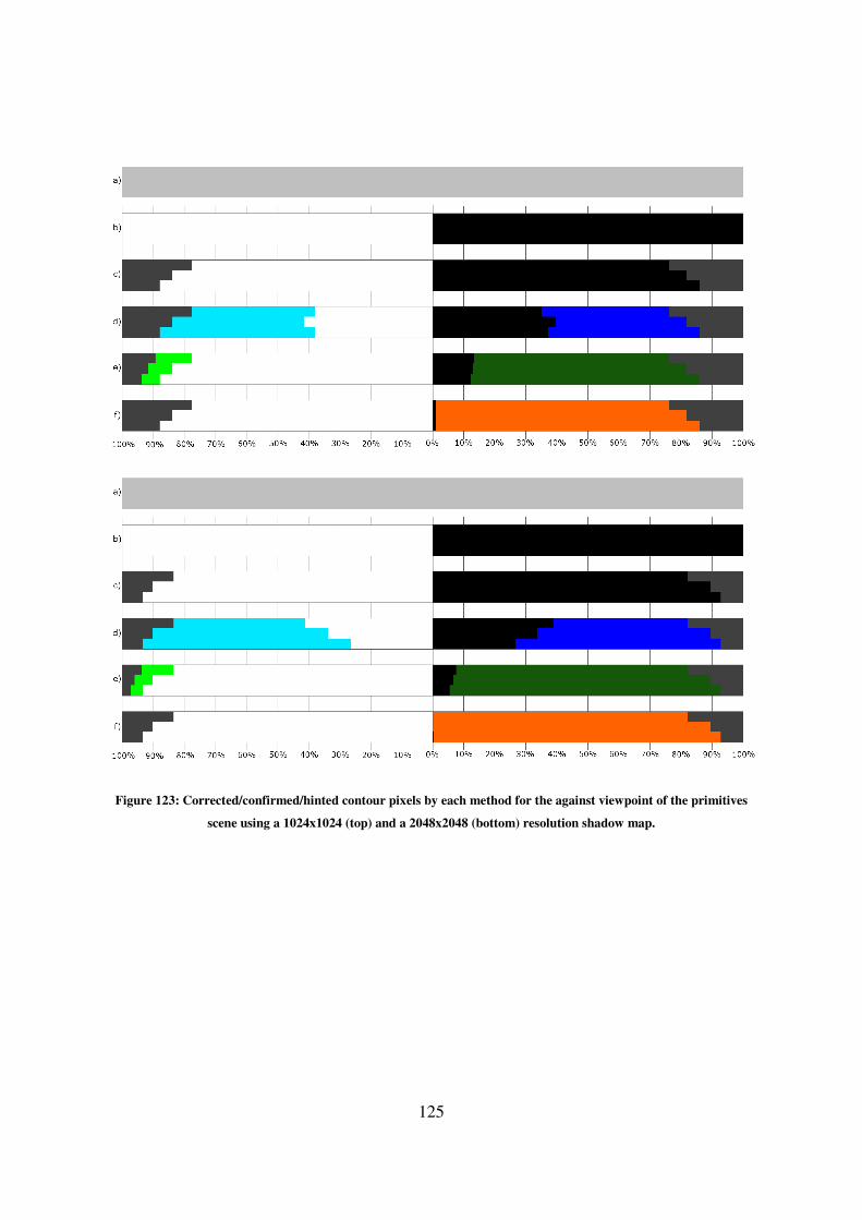
125
Figure 123: Corrected/confirmed/hinted contour pixels by each method for the against viewpoint of the primitives
scene using a 1024x1024 (top) and a 2048x2048 (bottom) resolution shadow map.
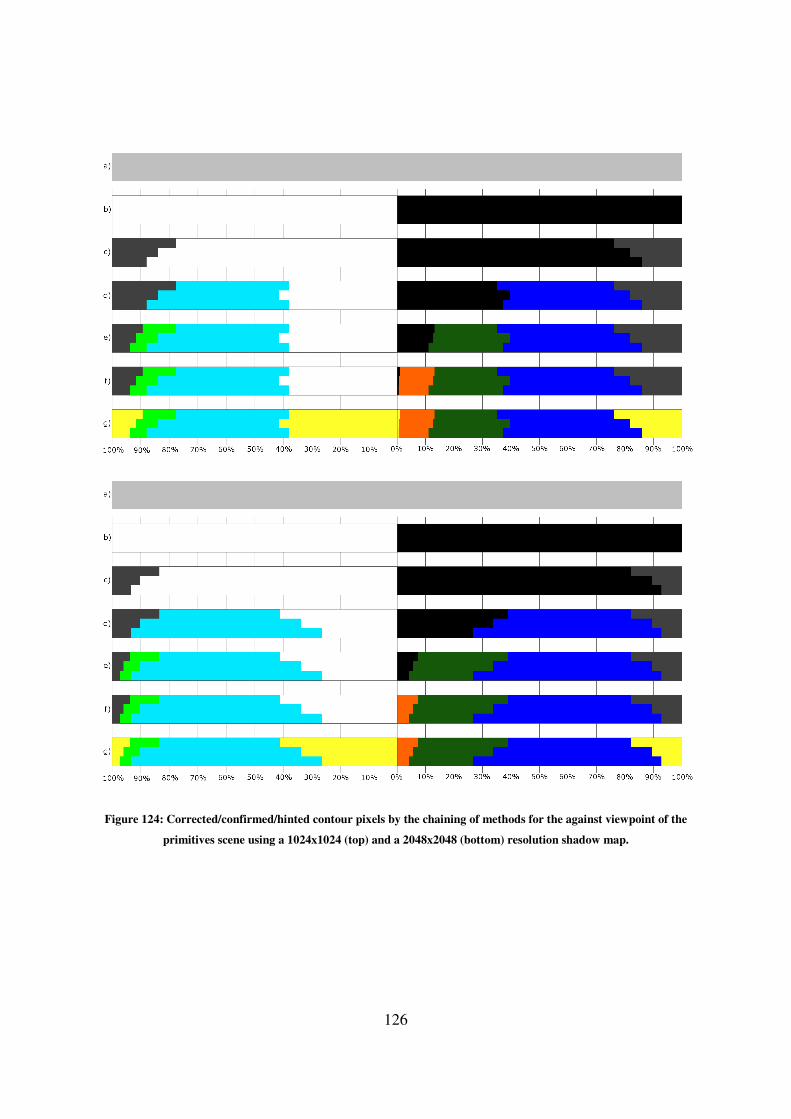
126
Figure 124: Corrected/confirmed/hinted contour pixels by the chaining of methods for the against viewpoint of the
primitives scene using a 1024x1024 (top) and a 2048x2048 (bottom) resolution shadow map.

127
Shadow Map
Resolution Approach
Contour Thickness
Two Pixels Four Pixels Six Pixels Whole Image
1024x1024
Pixels in
Contour 11229 22196 32998 1048576
Shadow Map 2582 (22.99%) 3799 (17.12%) 4272 (12.95%) 4497 (0.43%)
Single Texel 2559 (22.79%) 4499 (20.27%) 6021 (18.25%) 36323 (3.46%)
Neighbour
Texels (4
Neighbours)
1747 (15.56%) 3066 (13.81%) 3969 (12.03%) 12958 (1.24%)
Neighbour
Texels (9
Neighbours)
1352 (12.04%) 2367 (10.66%) 3048 (9.24%) 8768 (0.84%)
Adjacent
Geometry (One
Level)
1882 (16.76%) 2956 (13.32%) 3602 (10.92%) 8643 (0.82%)
Adjacent
Geometry
(Two Level)
1311 (11.68%) 1931 (8.70%) 2194 (6.65%) 2548 (0.24%)
2048x2048
Pixels in
Contour 11186 22079 32776 1048576
Shadow Map 1922 (17.18%) 2222 (10.06%) 2251 (6.87%) 2252 (0.21%)
Single Texel 1915 (17.12%) 3118 (14.12%) 3976 (12.13%) 20399 (1.95%)
Neighbour
Texels (4
Neighbours)
1000 (8.94%) 1561 (7.07%) 1832 (5.59%) 4181 (0.40%)
Neighbour
Texels (9
Neighbours)
776 (6.94%) 1169 (5.29%) 1340 (4.09%) 2731 (0.26%)
Adjacent
Geometry (One
Level)
1235 (11.04%) 1634 (7.40%) 1816 (5.54%) 3167 (0.30%)
Adjacent
Geometry
(Two Level)
940 (8.40%) 1103 (5.00%) 1135 (3.46%) 1237 (0.12%)
Table 46: Difference between the approaches that use ray-tracing and the actual ray-tracer for the against viewpoint
of the primitives scene.
Shadow Map Resolution Contour Thickness
Two Pixels Four Pixels Six Pixels
1024x1024 2582 of 4497 (57.42%) 3799 of 4497 (84.48%) 4272 of 4497 (95.00%)
2048x2048 1922 of 2252 (85.35%) 2222 of 2252 (98.67%) 2251 of 2252 (99.96%)
Table 47: Wrongly defined pixels in the shadow mapping result which are inside the contour in the against viewpoint
of the primitives scene.

128
Shadow Map Resolution Contour Thickness Pixel Shading
Light Shadow
1024x1024
Two Pixels 1256 of 5663 1326 of 5566
Four Pixels 1827 of 11300 1972 of 10896
Six Pixels 2035 of 16905 2237 of 16093
Whole Image 2118 of 918386 2379 of 130190
2048x2048
Two Pixels 932 of 5650 990 of 5536
Four Pixels 1082 of 11267 1140 of 10812
Six Pixels 1100 of 16833 1151 of 15943
Whole Image 1100 of 918595 1152 of 129981
Table 48: Pixels that the shadow map defines wrongly in the against viewpoint of the primitives scene, separated in
pixels defined in light and in shadow, compared to the total amount of pixels lighted in the same way.
Shadow
Map
Resolution
Contour
Thickness
Texel Coherence
Light Shadow
Confirmed Incorrectly
Confirmed Undecided Confirmed
Incorrectly
Confirmed Undecided
1024x1024
Two Pixels 2257
(39.86%) 1 (0.02%)
3406
(60.14%)
2289
(41.12%) 0 (0.00%)
3277
(58.88%)
Four Pixels 4788
(42.37%) 1 (0.01%)
6512
(57.63%)
4588
(42.11%) 0 (0.00%)
6308
(57.89%)
Six Pixels 8433
(49.88%) 1 (0.01%)
8472
(50.12%)
7873
(48.92%) 0 (0.00%)
8220
(51.08%)
Whole
Image
907090
(98.77%) 1 (0.00%)
11296
(1.23%)
119227
(91.58%) 1 (0.00%)
10963
(8.42%)
2048x2048
Two Pixels 2392
(42.34%) 1 (0.02%)
3258
(57.66%)
2387
(43.12%) 0 (0.00%)
3149
(56.88%)
Four Pixels 6390
(56.71%) 1 (0.01%)
4877
(43.29%)
6036
(55.83%) 0 (0.00%)
4776
(44.17%)
Six Pixels 11298
(67.12%) 1 (0.01%)
5535
(32.88%)
10524
(66.01%) 0 (0.00%)
5419
(33.99%)
Whole
Image
912949
(99.39%) 1 (0.00%)
5646
(0.61%)
124459
(95.75%) 1 (0.00%)
5522
(4.25%)
Table 49: Pixel confirmation when using texel coherence with four texels for the against viewpoint of the primitives
scene.
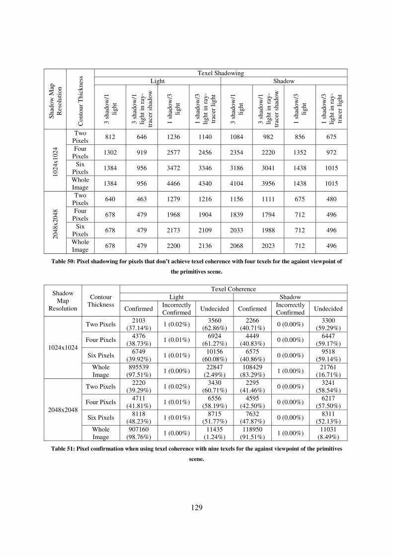
129
Sh
ado
w M
ap
Res
olu
tio
n
Co
nto
ur
Th
ick
nes
s Texel Shadowing
Light Shadow
3 s
had
ow
/1
lig
ht
3 s
had
ow
/1
lig
ht
in r
ay-
trac
er s
had
ow
1 s
had
ow
/3
lig
ht
1 s
had
ow
/3
lig
ht
in r
ay-
trac
er l
igh
t
3 s
had
ow
/1
lig
ht
3 s
had
ow
/1
lig
ht
in r
ay-
trac
er s
had
ow
1 s
had
ow
/3
lig
ht
1 s
had
ow
/3
lig
ht
in r
ay-
trac
er l
igh
t
10
24x
102
4
Two
Pixels 812 646 1236 1140 1084 982 856 675
Four
Pixels 1302 919 2577 2456 2354 2220 1352 972
Six
Pixels 1384 956 3472 3346 3186 3041 1438 1015
Whole
Image 1384 956 4466 4340 4104 3956 1438 1015
20
48x
204
8
Two
Pixels 640 463 1279 1216 1156 1111 675 480
Four
Pixels 678 479 1968 1904 1839 1794 712 496
Six
Pixels 678 479 2173 2109 2033 1988 712 496
Whole
Image 678 479 2200 2136 2068 2023 712 496
Table 50: Pixel shadowing for pixels that don’t achieve texel coherence with four texels for the against viewpoint of
the primitives scene.
Shadow
Map
Resolution
Contour
Thickness
Texel Coherence
Light Shadow
Confirmed Incorrectly
Confirmed Undecided Confirmed
Incorrectly
Confirmed Undecided
1024x1024
Two Pixels 2103
(37.14%) 1 (0.02%)
3560
(62.86%)
2266
(40.71%) 0 (0.00%)
3300
(59.29%)
Four Pixels 4376
(38.73%) 1 (0.01%)
6924
(61.27%)
4449
(40.83%) 0 (0.00%)
6447
(59.17%)
Six Pixels 6749
(39.92%) 1 (0.01%)
10156
(60.08%)
6575
(40.86%) 0 (0.00%)
9518
(59.14%)
Whole
Image
895539
(97.51%) 1 (0.00%)
22847
(2.49%)
108429
(83.29%) 1 (0.00%)
21761
(16.71%)
2048x2048
Two Pixels 2220
(39.29%) 1 (0.02%)
3430
(60.71%)
2295
(41.46%) 0 (0.00%)
3241
(58.54%)
Four Pixels 4711
(41.81%) 1 (0.01%)
6556
(58.19%)
4595
(42.50%) 0 (0.00%)
6217
(57.50%)
Six Pixels 8118
(48.23%) 1 (0.01%)
8715
(51.77%)
7632
(47.87%) 0 (0.00%)
8311
(52.13%)
Whole
Image
907160
(98.76%) 1 (0.00%)
11435
(1.24%)
118950
(91.51%) 1 (0.00%)
11031
(8.49%)
Table 51: Pixel confirmation when using texel coherence with nine texels for the against viewpoint of the primitives
scene.
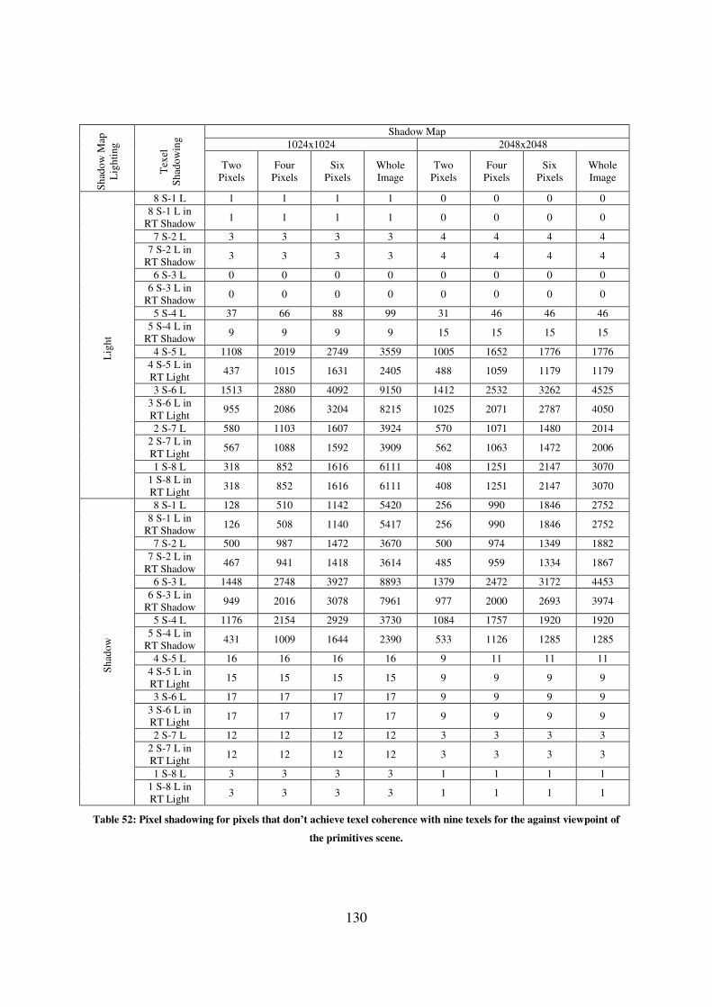
130
Sh
ado
w M
ap
Lig
hti
ng
Tex
el
Sh
ado
win
g Shadow Map
1024x1024 2048x2048
Two
Pixels
Four
Pixels
Six
Pixels
Whole
Image
Two
Pixels
Four
Pixels
Six
Pixels
Whole
Image
Lig
ht
8 S-1 L 1 1 1 1 0 0 0 0
8 S-1 L in
RT Shadow 1 1 1 1 0 0 0 0
7 S-2 L 3 3 3 3 4 4 4 4
7 S-2 L in
RT Shadow 3 3 3 3 4 4 4 4
6 S-3 L 0 0 0 0 0 0 0 0
6 S-3 L in
RT Shadow 0 0 0 0 0 0 0 0
5 S-4 L 37 66 88 99 31 46 46 46
5 S-4 L in
RT Shadow 9 9 9 9 15 15 15 15
4 S-5 L 1108 2019 2749 3559 1005 1652 1776 1776
4 S-5 L in
RT Light 437 1015 1631 2405 488 1059 1179 1179
3 S-6 L 1513 2880 4092 9150 1412 2532 3262 4525
3 S-6 L in
RT Light 955 2086 3204 8215 1025 2071 2787 4050
2 S-7 L 580 1103 1607 3924 570 1071 1480 2014
2 S-7 L in
RT Light 567 1088 1592 3909 562 1063 1472 2006
1 S-8 L 318 852 1616 6111 408 1251 2147 3070
1 S-8 L in
RT Light 318 852 1616 6111 408 1251 2147 3070
Sh
ado
w
8 S-1 L 128 510 1142 5420 256 990 1846 2752
8 S-1 L in
RT Shadow 126 508 1140 5417 256 990 1846 2752
7 S-2 L 500 987 1472 3670 500 974 1349 1882
7 S-2 L in
RT Shadow 467 941 1418 3614 485 959 1334 1867
6 S-3 L 1448 2748 3927 8893 1379 2472 3172 4453
6 S-3 L in
RT Shadow 949 2016 3078 7961 977 2000 2693 3974
5 S-4 L 1176 2154 2929 3730 1084 1757 1920 1920
5 S-4 L in
RT Shadow 431 1009 1644 2390 533 1126 1285 1285
4 S-5 L 16 16 16 16 9 11 11 11
4 S-5 L in
RT Light 15 15 15 15 9 9 9 9
3 S-6 L 17 17 17 17 9 9 9 9
3 S-6 L in
RT Light 17 17 17 17 9 9 9 9
2 S-7 L 12 12 12 12 3 3 3 3
2 S-7 L in
RT Light 12 12 12 12 3 3 3 3
1 S-8 L 3 3 3 3 1 1 1 1
1 S-8 L in
RT Light 3 3 3 3 1 1 1 1
Table 52: Pixel shadowing for pixels that don’t achieve texel coherence with nine texels for the against viewpoint of
the primitives scene.
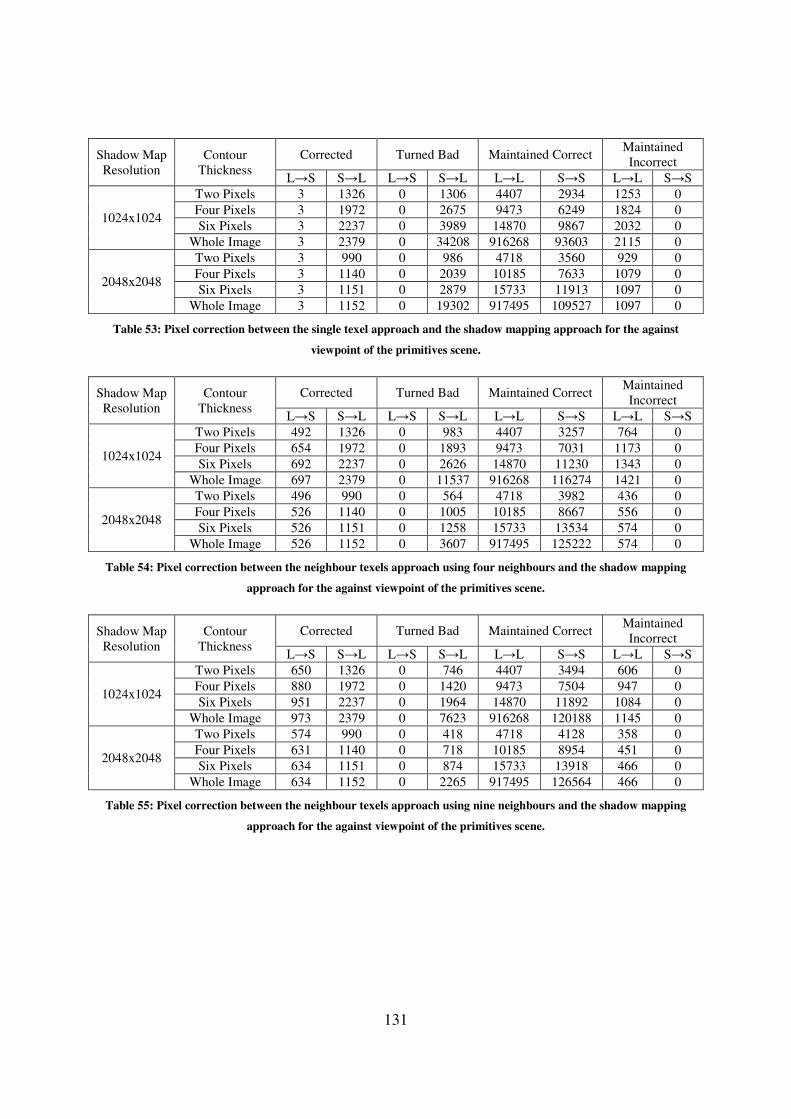
131
Shadow Map
Resolution
Contour
Thickness
Corrected Turned Bad Maintained Correct Maintained
Incorrect
L→S S→L L→S S→L L→L S→S L→L S→S
1024x1024
Two Pixels 3 1326 0 1306 4407 2934 1253 0
Four Pixels 3 1972 0 2675 9473 6249 1824 0
Six Pixels 3 2237 0 3989 14870 9867 2032 0
Whole Image 3 2379 0 34208 916268 93603 2115 0
2048x2048
Two Pixels 3 990 0 986 4718 3560 929 0
Four Pixels 3 1140 0 2039 10185 7633 1079 0
Six Pixels 3 1151 0 2879 15733 11913 1097 0
Whole Image 3 1152 0 19302 917495 109527 1097 0
Table 53: Pixel correction between the single texel approach and the shadow mapping approach for the against
viewpoint of the primitives scene.
Shadow Map
Resolution
Contour
Thickness
Corrected Turned Bad Maintained Correct Maintained
Incorrect
L→S S→L L→S S→L L→L S→S L→L S→S
1024x1024
Two Pixels 492 1326 0 983 4407 3257 764 0
Four Pixels 654 1972 0 1893 9473 7031 1173 0
Six Pixels 692 2237 0 2626 14870 11230 1343 0
Whole Image 697 2379 0 11537 916268 116274 1421 0
2048x2048
Two Pixels 496 990 0 564 4718 3982 436 0
Four Pixels 526 1140 0 1005 10185 8667 556 0
Six Pixels 526 1151 0 1258 15733 13534 574 0
Whole Image 526 1152 0 3607 917495 125222 574 0
Table 54: Pixel correction between the neighbour texels approach using four neighbours and the shadow mapping
approach for the against viewpoint of the primitives scene.
Shadow Map
Resolution
Contour
Thickness
Corrected Turned Bad Maintained Correct Maintained
Incorrect
L→S S→L L→S S→L L→L S→S L→L S→S
1024x1024
Two Pixels 650 1326 0 746 4407 3494 606 0
Four Pixels 880 1972 0 1420 9473 7504 947 0
Six Pixels 951 2237 0 1964 14870 11892 1084 0
Whole Image 973 2379 0 7623 916268 120188 1145 0
2048x2048
Two Pixels 574 990 0 418 4718 4128 358 0
Four Pixels 631 1140 0 718 10185 8954 451 0
Six Pixels 634 1151 0 874 15733 13918 466 0
Whole Image 634 1152 0 2265 917495 126564 466 0
Table 55: Pixel correction between the neighbour texels approach using nine neighbours and the shadow mapping
approach for the against viewpoint of the primitives scene.
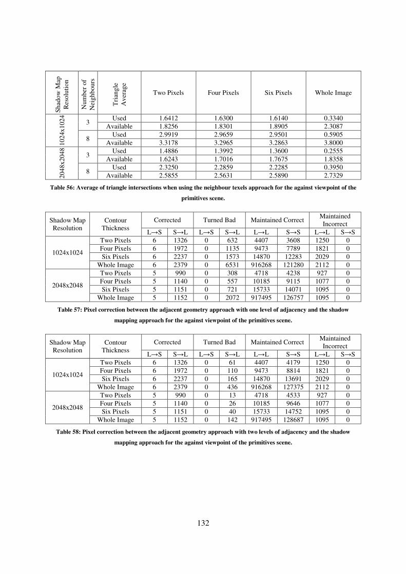
132
Sh
ado
w M
ap
Res
olu
tio
n
Nu
mb
er o
f
Nei
gh
bo
urs
Tri
ang
le
Av
erag
e
Two Pixels Four Pixels Six Pixels Whole Image
10
24x
102
4
3 Used 1.6412 1.6300 1.6140 0.3340
Available 1.8256 1.8301 1.8905 2.3087
8 Used 2.9919 2.9659 2.9501 0.5905
Available 3.3178 3.2965 3.2863 3.8000
20
48x
204
8
3 Used 1.4886 1.3992 1.3600 0.2555
Available 1.6243 1.7016 1.7675 1.8358
8 Used 2.3250 2.2859 2.2285 0.3950
Available 2.5855 2.5631 2.5890 2.7329
Table 56: Average of triangle intersections when using the neighbour texels approach for the against viewpoint of the
primitives scene.
Shadow Map
Resolution
Contour
Thickness
Corrected Turned Bad Maintained Correct Maintained
Incorrect
L→S S→L L→S S→L L→L S→S L→L S→S
1024x1024
Two Pixels 6 1326 0 632 4407 3608 1250 0
Four Pixels 6 1972 0 1135 9473 7789 1821 0
Six Pixels 6 2237 0 1573 14870 12283 2029 0
Whole Image 6 2379 0 6531 916268 121280 2112 0
2048x2048
Two Pixels 5 990 0 308 4718 4238 927 0
Four Pixels 5 1140 0 557 10185 9115 1077 0
Six Pixels 5 1151 0 721 15733 14071 1095 0
Whole Image 5 1152 0 2072 917495 126757 1095 0
Table 57: Pixel correction between the adjacent geometry approach with one level of adjacency and the shadow
mapping approach for the against viewpoint of the primitives scene.
Shadow Map
Resolution
Contour
Thickness
Corrected Turned Bad Maintained Correct Maintained
Incorrect
L→S S→L L→S S→L L→L S→S L→L S→S
1024x1024
Two Pixels 6 1326 0 61 4407 4179 1250 0
Four Pixels 6 1972 0 110 9473 8814 1821 0
Six Pixels 6 2237 0 165 14870 13691 2029 0
Whole Image 6 2379 0 436 916268 127375 2112 0
2048x2048
Two Pixels 5 990 0 13 4718 4533 927 0
Four Pixels 5 1140 0 26 10185 9646 1077 0
Six Pixels 5 1151 0 40 15733 14752 1095 0
Whole Image 5 1152 0 142 917495 128687 1095 0
Table 58: Pixel correction between the adjacent geometry approach with two levels of adjacency and the shadow
mapping approach for the against viewpoint of the primitives scene.

133
Sh
ado
w M
ap
Res
olu
tio
n
Ad
jace
ncy
Lev
el
Tri
ang
le
Av
erag
e
Two Pixels Four Pixels Six Pixels Whole Image
10
24x
102
4
One
Level
Used 2.2196 2.2274 2.2412 0.5277
Available 4.0000 4.0000 4.0000 4.0000
Two
Levels
Used 6.7627 7.1057 6.8057 1.6326
Available 12.1871 12.1625 12.1464 12.3744
20
48x
204
8
One
Level
Used 2.2410 2.2581 2.2689 0.5292
Available 4.0000 4.0000 4.0000 4.0000
Two
Levels
Used 6.7846 7.1057 6.8511 1.6362
Available 12.1098 12.0856 12.0785 12.3665
Table 59: Average of triangle intersections when using the adjacent geometry approach for the against viewpoint of
the primitives scene.

134
Contour Thickness Two Pixels Four Pixels Six Pixels Whole Image
Lighting L→S S→L L→S S→L L→S S→L L→S S→L
Sh
ado
w M
ap R
eso
luti
on
10
24x
102
4
Corrected by
Both 5 1326 5 1972 5 2237 5 2379
Turned Bad
by Both 0 54 0 92 0 130 0 241
Corrected by
Neighbour
Texels Only
645 0 875 0 946 0 968 0
Corrected by
Adjacent
Geometry
Only
1 0 1 0 1 0 1 0
Turned Bad
by
Neighbour
Texels Only
0 692 0 1328 0 1834 0 7382
Turned Bad
by Adjacent
Geometry
Only
0 7 0 18 0 35 0 195
20
48x
204
8
Corrected by
Both 5 990 5 1140 5 1151 5 1152
Turned Bad
by Both 0 10 0 11 0 13 0 29
Corrected by
Neighbour
Texels Only
569 0 626 0 629 0 629 0
Corrected by
Adjacent
Geometry
Only
0 0 0 0 0 0 0 0
Turned Bad
by
Neighbour
Texels Only
0 408 0 707 0 861 0 2236
Turned Bad
by Adjacent
Geometry
Only
0 3 0 15 0 27 0 113
Table 60: Pixel correction by the neighbour texels (9 texels) and the adjacent geometry (2 levels) approaches
separated by lighting change for the against viewpoint of the primitives scene.

135
Alg
ori
thm
Ste
p
Confirmations
and Errors
1024x1024 2048x2048
Two Pixels Four Pixels Six Pixel Two Pixels Four Pixels Six Pixel
Sh
ado
w M
ap
Total Contour
Pixels 11229 22196 32998 11186 22079 32776
Correct Light
Pixels
4407
(77.82%)
9473
(83.83%)
14870
(87.96%)
4718
(83.50%)
10185
(90.40%)
15733
(93.47%)
Correct Shadow
Pixels
4240
(76.18%)
8924
(81.90%)
13856
(86.10%)
4546
(82.12%)
9672
(89.46%)
14792
(92.78%)
Incorrect Light
Pixels
1256
(22.18%)
1827
(16.17%)
2035
(12.04%)
932
(16.50%)
1082
(9.60%)
1100
(6.53%)
Incorrect Shadow
Pixels
1326
(23.82%)
1972
(18.10%)
2237
(13.90%)
990
(17.88%)
1140
(10.54%)
1151
(7.22%)
Tex
el C
oh
eren
ce
Confirmations in
Light
2257
(39.86%)
4788
(42.37%)
8433
(49.88%)
2392
(42.34%)
6390
(56.71%)
11298
(67.12%)
Confirmations in
Shadow
2289
(41.12%)
4588
(42.11%)
7873
(48.92%)
2387
(43.12%)
6036
(55.83%)
10524
(66.01%)
Wrong
Confirmations in
Light
10 (0.00%) 10 (0.00%) 10 (0.00%) 10 (0.00%) 10 (0.00%) 10 (0.00%)
Wrong
Confirmations in
Shadow
0 (0.00%) 0 (0.00%) 0 (0.00%) 0 (0.00%) 0 (0.00%) 0 (0.00%)
Nei
gh
bo
uri
ng
Tex
els
Corrections from
Light
650
(11.48%)
880
(7.79%)
951
(5.63%)
574
(10.16%)
631
(5.60%)
634
(3.77%)
Confirmations in
Shadow
3508
(63.03%)
7534
(69.14%)
12078
(75.05%)
4131
(74.62%)
9051
(83.71%)
14118
(88.55%)
Ad
jace
nt
Geo
met
ry
Confirmations in
Shadow
4186
(75.21%)
8832
(81.06%)
13753
(85.46%)
4536
(81.94%)
9662
(89.36%)
14782
(92.72%)
Fin
al L
igh
tin
g Wrong
Confirmations in
Light
606
(10.70%)
947
(8.38%)
1084
(6.41%)
358
(6.34%)
451
(4.00%)
466
(2.77%)
Wrong
Confirmations in
Shadow
54 (0.97%) 92 (0.84%) 103
(0.64%) 10 (0.18%) 10 (0.09%) 10 (0.06%)
Table 61: Algorithm results of the against viewpoint of the primitives scene.
Below are the results for the “side” viewpoint of the “bench” scene.
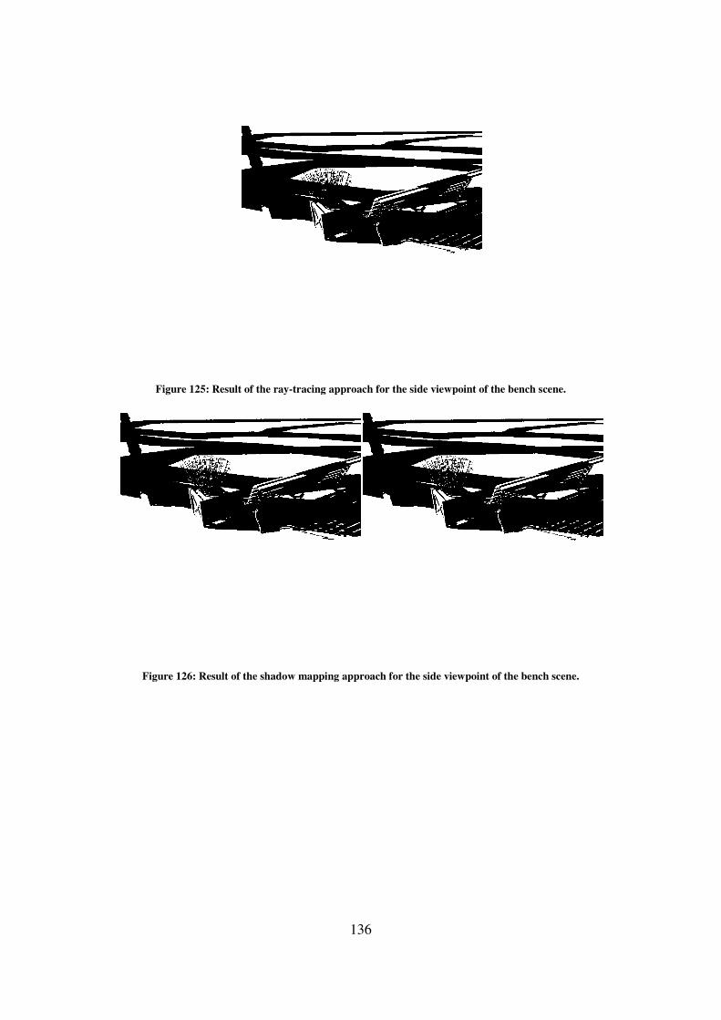
Figure 125: Result of the ray
Figure 126: Result of the shadow mapping a
136
: Result of the ray-tracing approach for the side viewpoint of the bench scene.
: Result of the shadow mapping approach for the side viewpoint of the bench
tracing approach for the side viewpoint of the bench scene.
bench scene.
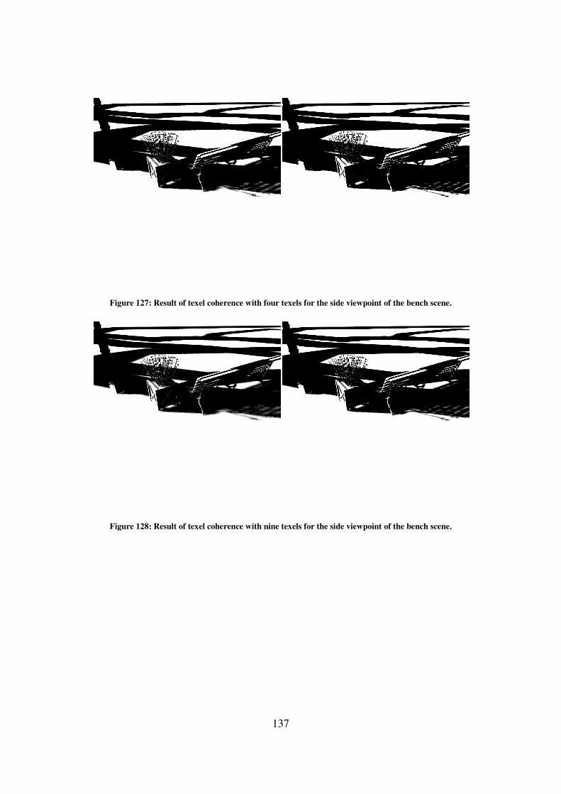
Figure 127: Result of texel coherence with four texels for
Figure 128: Result of texel coherence with nine texels for
137
: Result of texel coherence with four texels for the side viewpoint of the bench scene
: Result of texel coherence with nine texels for the side viewpoint of the bench scene
the side viewpoint of the bench scene.
the side viewpoint of the bench scene.
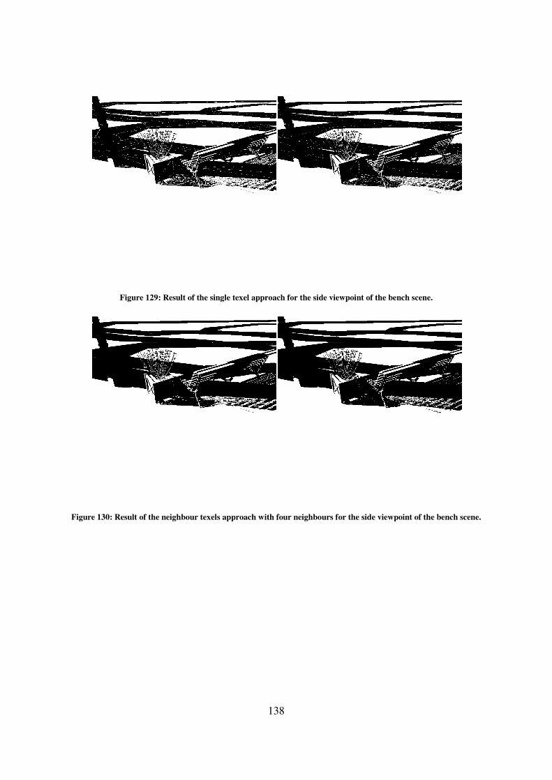
138
Figure 129: Result of the single texel approach for the side viewpoint of the bench scene.
Figure 130: Result of the neighbour texels approach with four neighbours for the side viewpoint of the bench scene.
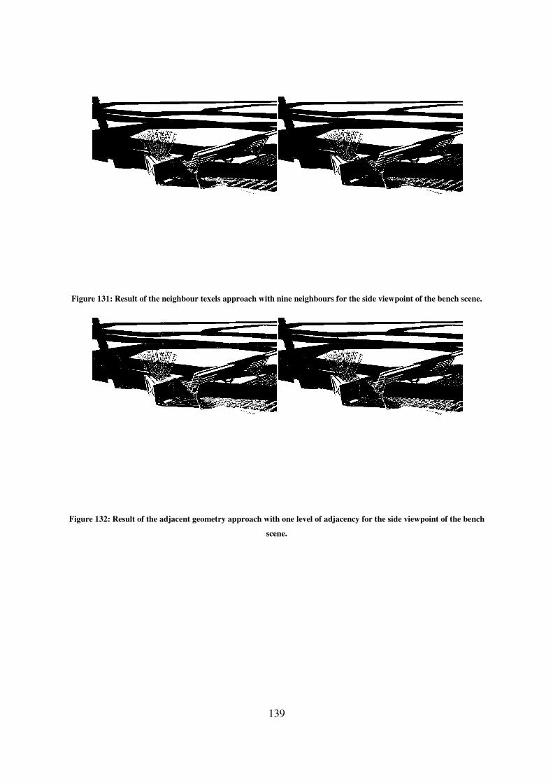
139
Figure 131: Result of the neighbour texels approach with nine neighbours for the side viewpoint of the bench scene.
Figure 132: Result of the adjacent geometry approach with one level of adjacency for the side viewpoint of the bench
scene.
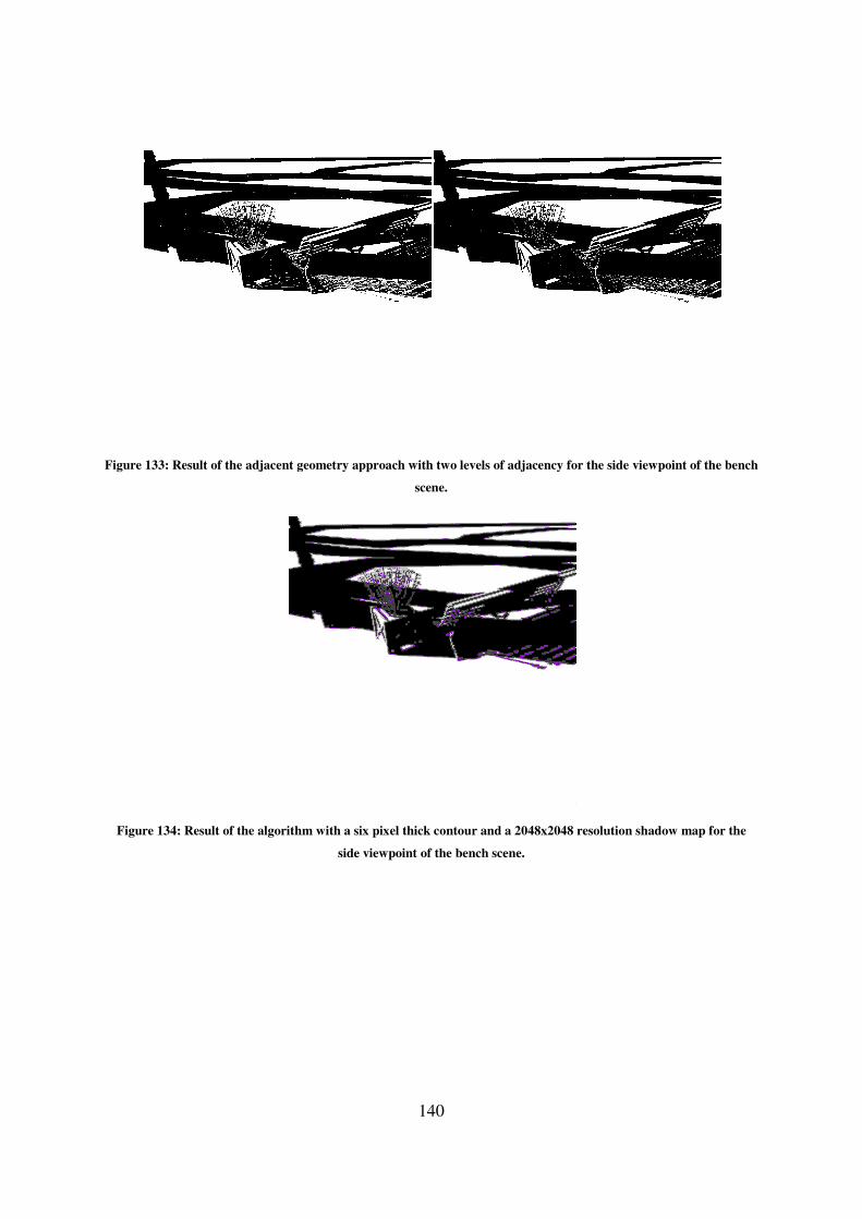
Figure 133: Result of the adjacent geometry
Figure 134: Result of the algorithm with a six pixel thick contour and a 2048x2048 resolution shadow map for the
140
adjacent geometry approach with two levels of adjacency for the side viewpoint of the bench
scene.
: Result of the algorithm with a six pixel thick contour and a 2048x2048 resolution shadow map for the
side viewpoint of the bench scene.
the side viewpoint of the bench
: Result of the algorithm with a six pixel thick contour and a 2048x2048 resolution shadow map for the

141
Figure 135: Corrected/confirmed/hinted contour pixels by each method for the side viewpoint of the bench scene
using a 1024x1024 (top) and a 2048x2048 (bottom) resolution shadow map.
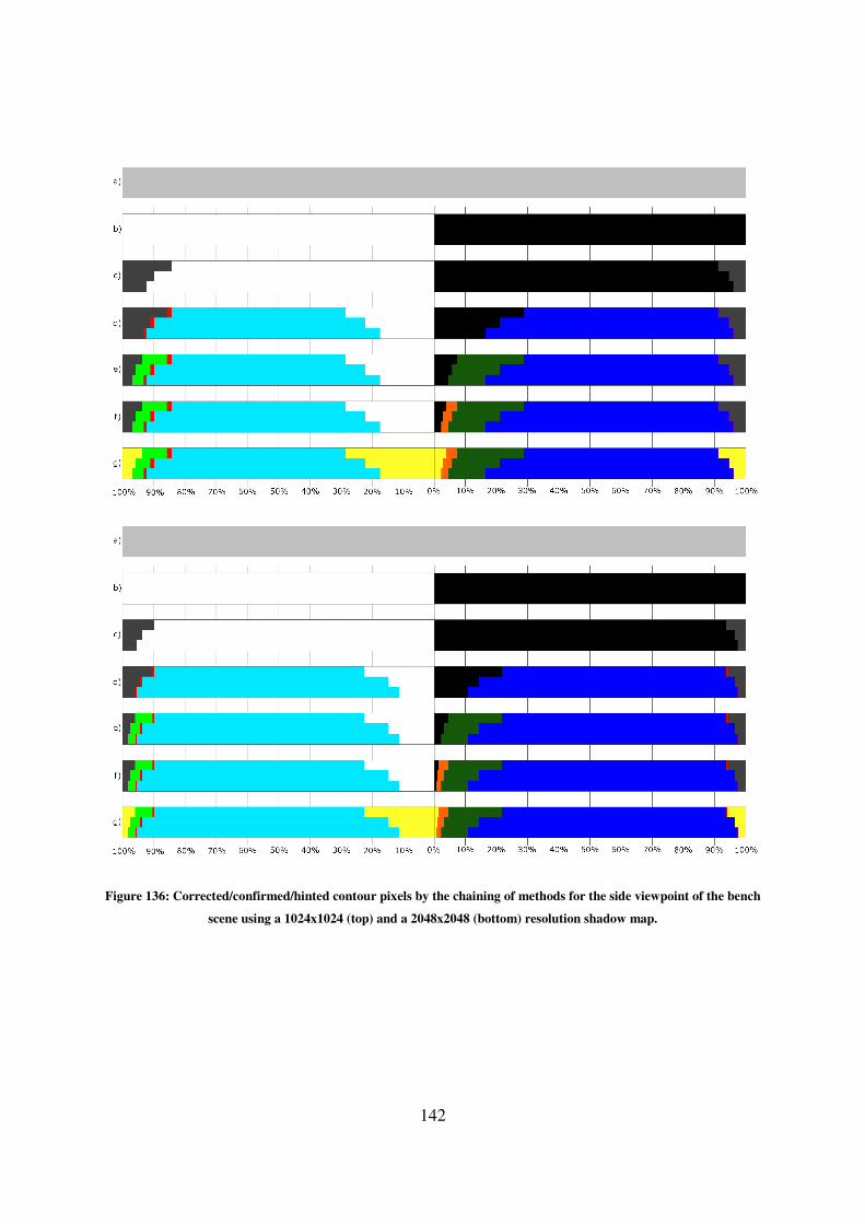
142
Figure 136: Corrected/confirmed/hinted contour pixels by the chaining of methods for the side viewpoint of the bench
scene using a 1024x1024 (top) and a 2048x2048 (bottom) resolution shadow map.
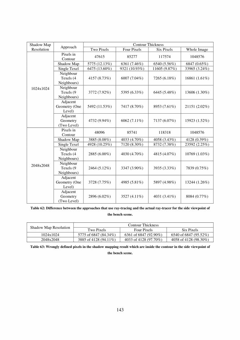
143
Shadow Map
Resolution Approach
Contour Thickness
Two Pixels Four Pixels Six Pixels Whole Image
1024x1024
Pixels in
Contour 47615 85277 117574 1048576
Shadow Map 5775 (12.13%) 6361 (7.46%) 6540 (5.56%) 6847 (0.65%)
Single Texel 6475 (13.60%) 9321 (10.93%) 11605 (9.87%) 33965 (3.24%)
Neighbour
Texels (4
Neighbours)
4157 (8.73%) 6007 (7.04%) 7265 (6.18%) 16861 (1.61%)
Neighbour
Texels (9
Neighbours)
3772 (7.92%) 5395 (6.33%) 6445 (5.48%) 13606 (1.30%)
Adjacent
Geometry (One
Level)
5492 (11.53%) 7417 (8.70%) 8953 (7.61%) 21151 (2.02%)
Adjacent
Geometry
(Two Level)
4732 (9.94%) 6062 (7.11%) 7137 (6.07%) 15923 (1.52%)
2048x2048
Pixels in
Contour 48096 85741 118318 1048576
Shadow Map 3885 (8.08%) 4033 (4.70%) 4058 (3.43%) 4128 (0.39%)
Single Texel 4928 (10.25%) 7120 (8.30%) 8732 (7.38%) 23592 (2.25%)
Neighbour
Texels (4
Neighbours)
2885 (6.00%) 4030 (4.70%) 4815 (4.07%) 10769 (1.03%)
Neighbour
Texels (9
Neighbours)
2464 (5.12%) 3347 (3.90%) 3935 (3.33%) 7839 (0.75%)
Adjacent
Geometry (One
Level)
3728 (7.75%) 4985 (5.81%) 5897 (4.98%) 13244 (1.26%)
Adjacent
Geometry
(Two Level)
2896 (6.02%) 3527 (4.11%) 4031 (3.41%) 8084 (0.77%)
Table 62: Difference between the approaches that use ray-tracing and the actual ray-tracer for the side viewpoint of
the bench scene.
Shadow Map Resolution Contour Thickness
Two Pixels Four Pixels Six Pixels
1024x1024 5775 of 6847 (84.34%) 6361 of 6847 (92.90%) 6540 of 6847 (95.52%)
2048x2048 3885 of 4128 (94.11%) 4033 of 4128 (97.70%) 4058 of 4128 (98.30%)
Table 63: Wrongly defined pixels in the shadow mapping result which are inside the contour in the side viewpoint of
the bench scene.

144
Shadow Map Resolution Contour Thickness Pixel Shading
Light Shadow
1024x1024
Two Pixels 3536 of 22450 2239 of 25165
Four Pixels 3837 of 38495 2524 of 46782
Six Pixels 3910 of 51325 2630 of 66249
Whole Image 3954 of 727189 2893 of 321387
2048x2048
Two Pixels 2286 of 22566 1599 of 25530
Four Pixels 2321 of 38321 1712 of 47420
Six Pixels 2324 of 51024 1734 of 67294
Whole Image 2333 of 726666 1795 of 321910
Table 64: Pixels that the shadow map defines wrongly in the side viewpoint of the bench scene, separated in pixels
defined in light and in shadow, compared to the total amount of pixels lighted in the same way.
Shadow
Map
Resolution
Contour
Thickness
Texel Coherence
Light Shadow
Confirmed Incorrectly
Confirmed Undecided Confirmed
Incorrectly
Confirmed Undecided
1024x1024
Two Pixels 12382
(55.15%)
347
(1.55%)
10068
(44.85%)
15717
(62.46%) 15 (0.06%)
9448
(37.54%)
Four Pixels 26537
(68.94%)
412
(1.07%)
11958
(31.06%)
34515
(73.78%) 72 (0.15%)
12267(26.2
2%)
Six Pixels 38867
(75.73%)
440
(0.86%)
12458
(24.27%)
52837
(79.76%)
116
(0.18%)
13412
(20.24%)
Whole
Image
714366
(98.24%)
451
(0.06%)
12823
(1.76%)
306506
(95.37%)
310
(0.10%)
14881
(4.63%)
2048x2048
Two Pixels 15340
(67.98%)
129
(0.57%)
7226
(32.02%)
18418
(72.14%) 33 (0.13%)
7112
(27.86%)
Four Pixels 30465
(79.50%)
144
(0.38%)
7856
(20.50%)
38912
(82.06%) 71 (0.15%)
8508
(17.94%)
Six Pixels 43081
(84.43%)
145
(0.28%)
7943
(15.57%)
58399
(86.78%) 86 (0.13%)
8895
(13.22%)
Whole
Image
718661
(98.90%)
145
(0.02%)
8005
(1.10%)
312737
(97.15%)
131
(0.04%)
9173
(2.85%)
Table 65: Pixel confirmation when using texel coherence with four texels for the side viewpoint of the bench scene.

145
Sh
ado
w M
ap
Res
olu
tio
n
Co
nto
ur
Th
ick
nes
s Texel Shadowing
Light Shadow
3 s
had
ow
/1
lig
ht
3 s
had
ow
/1
lig
ht
in r
ay-
trac
er s
had
ow
1 s
had
ow
/3
lig
ht
1 s
had
ow
/3
lig
ht
in r
ay-
trac
er l
igh
t
3 s
had
ow
/1
lig
ht
3 s
had
ow
/1
lig
ht
in r
ay-
trac
er s
had
ow
1 s
had
ow
/3
lig
ht
1 s
had
ow
/3
lig
ht
in r
ay-
trac
er l
igh
t
10
24x
102
4
Two
Pixels 2524 1590 3912 3414 4327 3895 1593 960
Four
Pixels 2718 1659 4945 4403 6166 5610 1766 984
Six
Pixels 2718 1659 5291 4739 7041 6440 1799 989
Whole
Image 2734 1670 5545 4980 8255 7595 1810 991
20
48x
204
8
Two
Pixels 1544 985 3003 2672 3327 3060 1226 713
Four
Pixels 1547 987 3431 3092 4265 3960 1263 715
Six
Pixels 1548 988 3495 3155 4531 4223 1279 716
Whole
Image 1556 993 3522 3182 4687 4373 1293 718
Table 66: Pixel shadowing for pixels that don’t achieve texel coherence with four texels for the side viewpoint of the
bench scene.
Shadow
Map
Resolution
Contour
Thickness
Texel Coherence
Light Shadow
Confirmed Incorrectly
Confirmed Undecided Confirmed
Incorrectly
Confirmed Undecided
1024x1024
Two Pixels 8247
(36.73%)
174
(0.78%)
14203
(63.27%)
12715
(50.53%) 2 (0.01%)
12450
(49.47%)
Four Pixels 19626
(50.98%)
183
(0.48%)
18869
(49.02%)
28276
(60.44%) 8 (0.02%)
18506
(39.56%)
Six Pixels 30488
(59.40%)
187
(0.36%)
20837
(40.60%)
44458
(67.11%) 16 (0.02%)
21791
(32.89%)
Whole
Image
704625
(96.90%)
198
(0.03%)
22564
(3.10%)
293499
(91.32%)
174
(0.05%)
27888
(8.68%)
2048x2048
Two Pixels 11762
(52.12%) 67 (0.30%)
10804
(47.88%)
15032
(58.88%) 4 (0.02%)
10498
(41.12%)
Four Pixels 25588
(66.77%) 75 (0.20%)
12733
(33.23%)
33488
(70.62%) 12 (0.03%)
13932
(29.38%)
Six Pixels 37864
(74.21%) 75 (0.15%)
13160
(25.79%)
52038
(77.33%) 18 (0.03%)
15256
(22.67%)
Whole
Image
713215
(98.15%) 75 (0.01%)
13451
(1.85%)
305286
(94.84%) 52 (0.02%)
16624
(5.16%)
Table 67: Pixel confirmation when using texel coherence with nine texels for the side viewpoint of the bench scene.
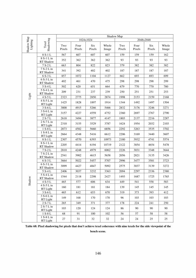
146
Sh
ado
w M
ap
Lig
hti
ng
Tex
el
Sh
ado
win
g Shadow Map
1024x1024 2048x2048
Two
Pixels
Four
Pixels
Six
Pixels
Whole
Image
Two
Pixels
Four
Pixels
Six
Pixels
Whole
Image
Lig
ht
8 S-1 L 567 607 607 607 159 159 159 162
8 S-1 L in
RT Shadow 352 362 362 362 93 93 93 93
7 S-2 L 663 804 822 823 379 382 382 382
7 S-2 L in
RT Shadow 341 392 402 402 187 187 187 187
6 S-3 L 857 1072 1104 1127 662 693 693 699
6 S-3 L in
RT Shadow 402 461 470 475 298 298 298 299
5 S-4 L 502 620 651 664 679 770 770 780
5 S-4 L in
RT Shadow 209 231 237 239 250 251 251 253
4 S-5 L 2323 2775 2850 2874 1998 2153 2159 2168
4 S-5 L in
RT Light 1425 1828 1897 1914 1344 1492 1497 1504
3 S-6 L 3800 4915 5266 5466 2832 3176 3246 3271
3 S-6 L in
RT Light 3157 4227 4559 4752 2360 2697 2767 2790
2 S-7 L 2618 3494 3877 4147 1803 2137 2216 2287
2 S-7 L in
RT Light 2310 3155 3529 3787 1624 1954 2032 2103
1 S-8 L 2873 4582 5660 6856 2292 3263 3535 3702
1 S-8 L in
RT Light 2664 4348 5416 6612 2206 3169 3440 3607
Sh
ado
w
8 S-1 L 2307 4570 6393 10973 2180 3932 4741 5574
8 S-1 L in
RT Shadow 2205 4414 6194 10719 2122 3854 4654 5478
7 S-2 L 2810 4248 4979 6062 2226 3031 3348 3644
7 S-2 L in
RT Shadow 2541 3902 4615 5658 2056 2821 3135 3426
6 S-3 L 3664 5022 5457 5707 2996 3477 3581 3723
6 S-3 L in
RT Shadow 3099 4427 4847 5092 2575 3037 3139 3272
5 S-4 L 2406 3037 3232 3363 2094 2297 2336 2380
5 S-4 L in
RT Shadow 1544 2118 2298 2427 1493 1687 1725 1765
4 S-5 L 465 577 606 634 449 541 558 583
4 S-5 L in
RT Light 160 181 181 184 139 145 145 145
3 S-6 L 465 612 653 670 319 373 393 412
3 S-6 L in
RT Light 149 168 170 170 96 103 103 103
2 S-7 L 265 349 371 377 178 224 241 250
2 S-7 L in
RT Light 103 120 124 124 86 90 90 90
1 S-8 L 68 91 100 102 56 57 58 58
1 S-8 L in
RT Light 27 31 32 32 24 24 25 25
Table 68: Pixel shadowing for pixels that don’t achieve texel coherence with nine texels for the side viewpoint of the
bench scene.

147
Shadow Map
Resolution
Contour
Thickness
Corrected Turned Bad Maintained Correct Maintained
Incorrect
L→S S→L L→S S→L L→L S→S L→L S→S
1024x1024
Two Pixels 64 2239 0 3003 18914 19923 3472 0
Four Pixels 64 2524 0 5548 34658 38710 3773 0
Six Pixels 64 2630 0 7759 47415 55860 3846 0
Whole Image 64 2893 0 30075 723235 288419 3890 0
2048x2048
Two Pixels 56 1599 0 2698 20280 21233 2230 0
Four Pixels 56 1712 0 4855 36000 40853 2265 0
Six Pixels 56 1734 0 6464 48700 59096 2268 0
Whole Image 56 1795 0 21315 724333 298800 2277 0
Table 69: Pixel correction between the single texel approach and the shadow mapping approach for the side
viewpoint of the bench scene.
Shadow Map
Resolution
Contour
Thickness
Corrected Turned Bad Maintained Correct Maintained
Incorrect
L→S S→L L→S S→L L→L S→S L→L S→S
1024x1024
Two Pixels 1622 2239 0 2243 18914 20683 1914 0
Four Pixels 1661 2524 0 3831 34658 40427 2176 0
Six Pixels 1669 2630 0 5024 47415 58595 2241 0
Whole Image 1681 2893 0 14588 723235 303906 2273 0
2048x2048
Two Pixels 1127 1599 0 1726 20280 22205 1159 0
Four Pixels 1133 1712 0 2842 36000 42866 1188 0
Six Pixels 1134 1734 0 3625 48700 61935 1190 0
Whole Image 1140 1795 0 9576 724333 310539 1193 0
Table 70: Pixel correction between the neighbour texels approach using four neighbours and the shadow mapping
approach for the side viewpoint of the bench scene.
Shadow Map
Resolution
Contour
Thickness
Corrected Turned Bad Maintained Correct Maintained
Incorrect
L→S S→L L→S S→L L→L S→S L→L S→S
1024x1024
Two Pixels 1795 2239 0 2031 18914 20895 1741 0
Four Pixels 1854 2524 0 3412 34658 40846 1983 0
Six Pixels 1863 2630 0 4398 47415 59221 2047 0
Whole Image 1879 2893 0 11531 723235 306963 2075 0
2048x2048
Two Pixels 1266 1599 0 1444 20280 22487 1020 0
Four Pixels 1276 1712 0 2302 36000 43406 1045 0
Six Pixels 1277 1734 0 2888 48700 62672 1047 0
Whole Image 1284 1795 0 6790 724333 313325 1049 0
Table 71: Pixel correction between the neighbour texels approach using nine neighbours and the shadow mapping
approach for the side viewpoint of the bench scene.
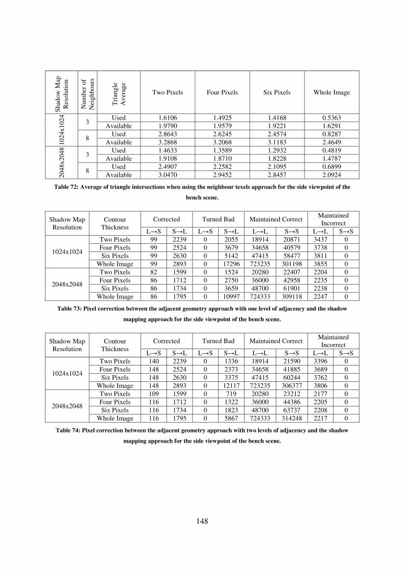
148
Sh
ado
w M
ap
Res
olu
tio
n
Nu
mb
er o
f
Nei
gh
bo
urs
Tri
ang
le
Av
erag
e
Two Pixels Four Pixels Six Pixels Whole Image
10
24x
102
4
3 Used 1.6106 1.4925 1.4168 0.5363
Available 1.9790 1.9579 1.9221 1.6291
8 Used 2.8643 2.6245 2.4574 0.8287
Available 3.2868 3.2068 3.1183 2.4649
20
48x
204
8
3 Used 1.4633 1.3589 1.2932 0.4819
Available 1.9108 1.8710 1.8228 1.4787
8 Used 2.4907 2.2582 2.1095 0.6899
Available 3.0470 2.9452 2.8457 2.0924
Table 72: Average of triangle intersections when using the neighbour texels approach for the side viewpoint of the
bench scene.
Shadow Map
Resolution
Contour
Thickness
Corrected Turned Bad Maintained Correct Maintained
Incorrect
L→S S→L L→S S→L L→L S→S L→L S→S
1024x1024
Two Pixels 99 2239 0 2055 18914 20871 3437 0
Four Pixels 99 2524 0 3679 34658 40579 3738 0
Six Pixels 99 2630 0 5142 47415 58477 3811 0
Whole Image 99 2893 0 17296 723235 301198 3855 0
2048x2048
Two Pixels 82 1599 0 1524 20280 22407 2204 0
Four Pixels 86 1712 0 2750 36000 42958 2235 0
Six Pixels 86 1734 0 3659 48700 61901 2238 0
Whole Image 86 1795 0 10997 724333 309118 2247 0
Table 73: Pixel correction between the adjacent geometry approach with one level of adjacency and the shadow
mapping approach for the side viewpoint of the bench scene.
Shadow Map
Resolution
Contour
Thickness
Corrected Turned Bad Maintained Correct Maintained
Incorrect
L→S S→L L→S S→L L→L S→S L→L S→S
1024x1024
Two Pixels 140 2239 0 1336 18914 21590 3396 0
Four Pixels 148 2524 0 2373 34658 41885 3689 0
Six Pixels 148 2630 0 3375 47415 60244 3762 0
Whole Image 148 2893 0 12117 723235 306377 3806 0
2048x2048
Two Pixels 109 1599 0 719 20280 23212 2177 0
Four Pixels 116 1712 0 1322 36000 44386 2205 0
Six Pixels 116 1734 0 1823 48700 63737 2208 0
Whole Image 116 1795 0 5867 724333 314248 2217 0
Table 74: Pixel correction between the adjacent geometry approach with two levels of adjacency and the shadow
mapping approach for the side viewpoint of the bench scene.

149
Sh
ado
w M
ap
Res
olu
tio
n
Ad
jace
ncy
Lev
el
Tri
ang
le
Av
erag
e
Two Pixels Four Pixels Six Pixels Whole Image
10
24x
102
4
One
Level
Used 2.4328 2.4567 2.4731 1.2381
Available 3.8549 3.8641 3.8724 3.9006
Two
Levels
Used 7.8846 7.9396 8.0098 4.0985
Available 12.4934 12.4881 12.5415 12.9121
20
48x
204
8
One
Level
Used 2.4726 2.5012 2.5187 1.2440
Available 3.8447 3.8582 3.8682 3.8978
Two
Levels
Used 7.8913 7.9598 8.0509 4.1005
Available 12.2702 12.2784 12.3648 12.8484
Table 75: Average of triangle intersections when using the adjacent geometry approach for the side viewpoint of the
bench scene.

150
Contour Thickness Two Pixels Four Pixels Six Pixels Whole Image
Lighting L→S S→L L→S S→L L→S S→L L→S S→L
Sh
ado
w M
ap R
eso
luti
on
10
24x
102
4
Corrected by
Both 82 2239 86 2524 86 2630 86 2893
Turned Bad
by Both 0 1072 0 1793 0 2386 0 6359
Corrected by
Neighbour
Texels Only
1713 0 1768 0 1777 0 1793 0
Corrected by
Adjacent
Geometry
Only
58 0 62 0 62 0 62 0
Turned Bad
by
Neighbour
Texels Only
0 959 0 1619 0 2012 0 5172
Turned Bad
by Adjacent
Geometry
Only
0 264 0 580 0 989 0 5758
20
48x
204
8
Corrected by
Both 76 1599 78 1712 78 1734 78 1795
Turned Bad
by Both 0 487 0 831 0 1085 0 2575
Corrected by
Neighbour
Texels Only
1190 0 1198 0 1199 0 1206 0
Corrected by
Adjacent
Geometry
Only
33 0 38 0 38 0 38 0
Turned Bad
by
Neighbour
Texels Only
0 957 0 1471 0 1803 0 4215
Turned Bad
by Adjacent
Geometry
Only
0 232 0 491 0 738 0 3292
Table 76: Pixel correction by the neighbour texels (9 texels) and the adjacent geometry (2 levels) approaches
separated by lighting change for the side viewpoint of the bench scene.
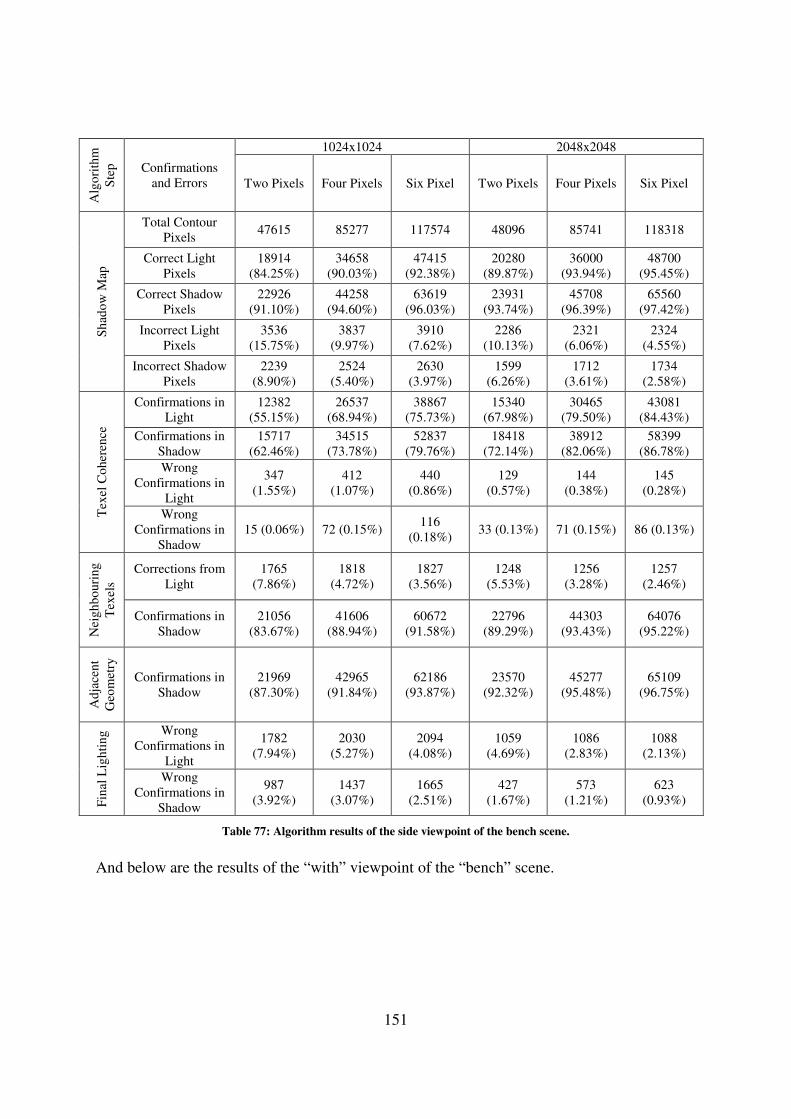
151
Alg
ori
thm
Ste
p
Confirmations
and Errors
1024x1024 2048x2048
Two Pixels Four Pixels Six Pixel Two Pixels Four Pixels Six Pixel
Sh
ado
w M
ap
Total Contour
Pixels 47615 85277 117574 48096 85741 118318
Correct Light
Pixels
18914
(84.25%)
34658
(90.03%)
47415
(92.38%)
20280
(89.87%)
36000
(93.94%)
48700
(95.45%)
Correct Shadow
Pixels
22926
(91.10%)
44258
(94.60%)
63619
(96.03%)
23931
(93.74%)
45708
(96.39%)
65560
(97.42%)
Incorrect Light
Pixels
3536
(15.75%)
3837
(9.97%)
3910
(7.62%)
2286
(10.13%)
2321
(6.06%)
2324
(4.55%)
Incorrect Shadow
Pixels
2239
(8.90%)
2524
(5.40%)
2630
(3.97%)
1599
(6.26%)
1712
(3.61%)
1734
(2.58%)
Tex
el C
oh
eren
ce
Confirmations in
Light
12382
(55.15%)
26537
(68.94%)
38867
(75.73%)
15340
(67.98%)
30465
(79.50%)
43081
(84.43%)
Confirmations in
Shadow
15717
(62.46%)
34515
(73.78%)
52837
(79.76%)
18418
(72.14%)
38912
(82.06%)
58399
(86.78%)
Wrong
Confirmations in
Light
347
(1.55%)
412
(1.07%)
440
(0.86%)
129
(0.57%)
144
(0.38%)
145
(0.28%)
Wrong
Confirmations in
Shadow
15 (0.06%) 72 (0.15%) 116
(0.18%) 33 (0.13%) 71 (0.15%) 86 (0.13%)
Nei
gh
bo
uri
ng
Tex
els
Corrections from
Light
1765
(7.86%)
1818
(4.72%)
1827
(3.56%)
1248
(5.53%)
1256
(3.28%)
1257
(2.46%)
Confirmations in
Shadow
21056
(83.67%)
41606
(88.94%)
60672
(91.58%)
22796
(89.29%)
44303
(93.43%)
64076
(95.22%)
Ad
jace
nt
Geo
met
ry
Confirmations in
Shadow
21969
(87.30%)
42965
(91.84%)
62186
(93.87%)
23570
(92.32%)
45277
(95.48%)
65109
(96.75%)
Fin
al L
igh
tin
g Wrong
Confirmations in
Light
1782
(7.94%)
2030
(5.27%)
2094
(4.08%)
1059
(4.69%)
1086
(2.83%)
1088
(2.13%)
Wrong
Confirmations in
Shadow
987
(3.92%)
1437
(3.07%)
1665
(2.51%)
427
(1.67%)
573
(1.21%)
623
(0.93%)
Table 77: Algorithm results of the side viewpoint of the bench scene.
And below are the results of the “with” viewpoint of the “bench” scene.
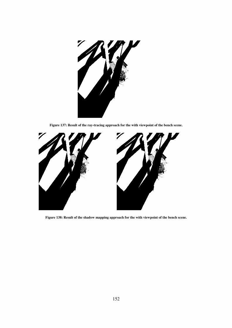
Figure 137: Result of the ray
Figure 138: Result of the shadow mapping approach for the
152
: Result of the ray-tracing approach for the with viewpoint of the bench scene.
: Result of the shadow mapping approach for the with viewpoint of the
tracing approach for the with viewpoint of the bench scene.
viewpoint of the bench scene.

Figure 139: Result of texel coherence with four texels for
Figure 140: Result of texel coherence with nine texels for
153
: Result of texel coherence with four texels for the with viewpoint of the bench scene
: Result of texel coherence with nine texels for the with viewpoint of the bench scene
the with viewpoint of the bench scene.
the with viewpoint of the bench scene.
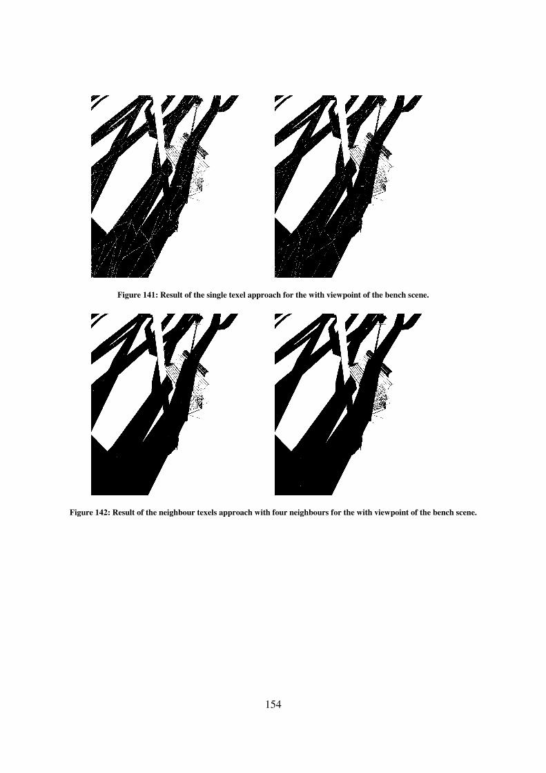
154
Figure 141: Result of the single texel approach for the with viewpoint of the bench scene.
Figure 142: Result of the neighbour texels approach with four neighbours for the with viewpoint of the bench scene.
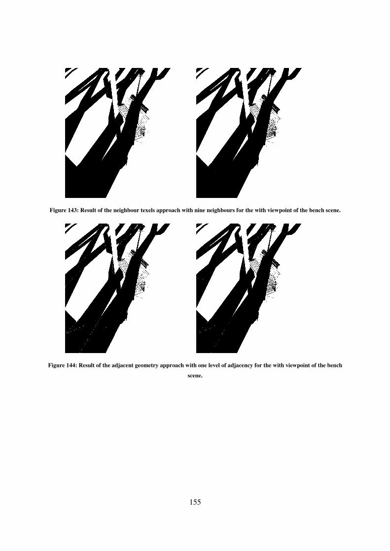
155
Figure 143: Result of the neighbour texels approach with nine neighbours for the with viewpoint of the bench scene.
Figure 144: Result of the adjacent geometry approach with one level of adjacency for the with viewpoint of the bench
scene.
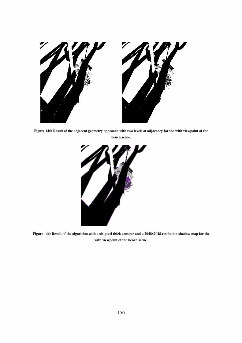
Figure 145: Result of the adjacent geometry
Figure 146: Result of the algorithm with a six pixel thick contour and a 2048x2048 resolution shadow map for the
156
adjacent geometry approach with two levels of adjacency for the with viewpoint of the
bench scene.
: Result of the algorithm with a six pixel thick contour and a 2048x2048 resolution shadow map for the
with viewpoint of the bench scene.
the with viewpoint of the
: Result of the algorithm with a six pixel thick contour and a 2048x2048 resolution shadow map for the
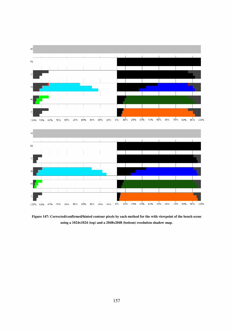
157
Figure 147: Corrected/confirmed/hinted contour pixels by each method for the with viewpoint of the bench scene
using a 1024x1024 (top) and a 2048x2048 (bottom) resolution shadow map.

158
Figure 148: Corrected/confirmed/hinted contour pixels by the chaining of methods for the with viewpoint of the
bench scene using a 1024x1024 (top) and a 2048x2048 (bottom) resolution shadow map.

159
Shadow Map
Resolution Approach
Contour Thickness
Two Pixels Four Pixels Six Pixels Whole Image
1024x1024
Pixels in
Contour 36910 65811 91380 1048576
Shadow Map 6268 (16.98%) 6664 (10.13%) 6721 (7.36%) 6799 (0.65%)
Single Texel 6643 (18.00%) 8439 (12.82%) 9284 (10.16%) 20216 (1.93%)
Neighbour
Texels (4
Neighbours)
3783 (10.25%) 4853 (7.37%) 5179 (5.67%) 5591 (0.53%)
Neighbour
Texels (9
Neighbours)
3298 (8.94%) 4247 (6.45%) 4535 (4.96%) 4801 (0.46%)
Adjacent
Geometry (One
Level)
5546 (15.03%) 6669 (10.13%) 7076 (7.74%) 8278 (0.79%)
Adjacent
Geometry
(Two Level)
4833 (13.09%) 5619 (8.54%) 5911 (6.47%) 6800 (0.65%)
2048x2048
Pixels in
Contour 36758 65457 91013 1048576
Shadow Map 3603 (9.80%) 3674 (5.61%) 3684 (4.05%) 3710 (0.35%)
Single Texel 4811 (13.09%) 6084 (9.29%) 6629 (7.28%) 12081 (1.15%)
Neighbour
Texels (4
Neighbours)
2586 (7.04%) 3376 (5.16%) 3629 (3.99%) 3754 (0.36%)
Neighbour
Texels (9
Neighbours)
2110 (5.74%) 2760 (4.22%) 2985 (3.28%) 3063 (0.29%)
Adjacent
Geometry (One
Level)
3543 (9.64%) 4288 (6.55%) 4577 (5.03%) 5101 (0.49%)
Adjacent
Geometry
(Two Level)
2679 (7.29%) 3079 (4.70%) 3231 (3.55%) 3639 (0.35%)
Table 78: Difference between the approaches that use ray-tracing and the actual ray-tracer for the with viewpoint of
the bench scene.
Shadow Map Resolution Contour Thickness
Two Pixels Four Pixels Six Pixels
1024x1024 6268 of 6799 (92.19%) 6664 of 6799 (98.01%) 6721 of 6799 (98.85%)
2048x2048 3603 of 3710 (97.12%) 3674 of 3710 (99.03%) 3684 of 3710 (99.30%)
Table 79: Wrongly defined pixels in the shadow mapping result which are inside the contour in the with viewpoint of
the bench scene.

160
Shadow Map Resolution Contour Thickness Pixel Shading
Light Shadow
1024x1024
Two Pixels 3464 of 18814 2804 of 18096
Four Pixels 3648 of 34230 3016 of 31581
Six Pixels 3663 of 47648 3058 of 43732
Whole Image 3710 of 681367 3089 of 367209
2048x2048
Two Pixels 1967 of 18481 1636 of 18277
Four Pixels 1987 of 33605 1687 of 31852
Six Pixels 1991 of 46917 1693 of 44096
Whole Image 2010 of 681056 1700 of 367520
Table 80: Pixels that the shadow map defines wrongly in the with viewpoint of the bench scene, separated in pixels
defined in light and in shadow, compared to the total amount of pixels lighted in the same way.
Shadow
Map
Resolution
Contour
Thickness
Texel Coherence
Light Shadow
Confirmed Incorrectly
Confirmed Undecided Confirmed
Incorrectly
Confirmed Undecided
1024x1024
Two Pixels 7381
(39.23%)
390
(2.07%)
11433
(60.77%)
6585
(36.39%) 43 (0.24%)
11511
(63.61%)
Four Pixels 20741
(60.59%)
438
(1.28%)
13489
(39.41%)
17755
(56.22%)
111
(0.35%)
13826
(43.78%)
Six Pixels 33681
(70.69%)
449
(0.94%)
13967
(29.31%)
29414
(67.26%)
140
(0.32%)
14318
(32.74%)
Whole
Image
667121
(97.91%)
456
(0.07%)
14246
(2.09%)
352645
(96.03%)
143
(0.04%)
14564
(3.97%)
2048x2048
Two Pixels 11032
(59.69%)
104
(0.56%)
7449
(40.31%)
10280
(56.25%) 31 (0.17%)
7997
(43.75%)
Four Pixels 25827
(76.85%)
122
(0.36%)
7778
(23.15%)
23227
(72.92%) 74 (0.23%)
8625
(27.08%)
Six Pixels 39120
(83.38%)
126
(0.27%)
7797
(16.62%)
35399
(80.28%) 78 (0.18%)
8697
(19.72%)
Whole
Image
673171
(98.84%)
127
(0.02%)
7885
(1.16%)
358774
(97.62%) 78 (0.02%)
8746
(2.38%)
Table 81: Pixel confirmation when using texel coherence with four texels for the with viewpoint of the bench scene.
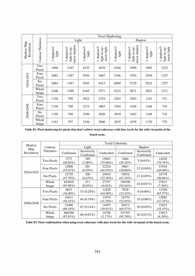
161
Sh
ado
w M
ap
Res
olu
tio
n
Co
nto
ur
Th
ick
nes
s Texel Shadowing
Light Shadow
3 s
had
ow
/1
lig
ht
3 s
had
ow
/1
lig
ht
in r
ay-
trac
er s
had
ow
1 s
had
ow
/3
lig
ht
1 s
had
ow
/3
lig
ht
in r
ay-
trac
er l
igh
t
3 s
had
ow
/1
lig
ht
3 s
had
ow
/1
lig
ht
in r
ay-
trac
er s
had
ow
1 s
had
ow
/3
lig
ht
1 s
had
ow
/3
lig
ht
in r
ay-
trac
er l
igh
t
10
24x
102
4
Two
Pixels 1960 1347 4325 3839 4304 3999 1903 1222
Four
Pixels 2082 1387 5594 5067 5746 5392 2030 1257
Six
Pixels 2084 1387 5943 5413 6089 5729 2032 1257
Whole
Image 2100 1399 6105 5571 6233 5871 2051 1271
20
48x
204
8
Two
Pixels 1150 789 3022 2754 3203 3052 1161 733
Four
Pixels 1150 789 3273 3003 3584 3428 1168 734
Six
Pixels 1150 789 3290 3020 3619 3462 1168 734
Whole
Image 1161 797 3336 3066 3635 3478 1170 735
Table 82: Pixel shadowing for pixels that don’t achieve texel coherence with four texels for the with viewpoint of the
bench scene.
Shadow
Map
Resolution
Contour
Thickness
Texel Coherence
Light Shadow
Confirmed Incorrectly
Confirmed Undecided Confirmed
Incorrectly
Confirmed Undecided
1024x1024
Two Pixels 3771
(20.04%)
189
(1.00%)
15043
(79.96%)
3666
(20.26%) 5 (0.03%)
14430
(79.74%)
Four Pixels 12006
(35.07%)
201
(0.59%)
22224
(64.93%)
9663
(30.60%) 12 (0.04%)
21918
(69.40%)
Six Pixels 22729
(47.70%)
206
(0.43%)
24919
(52.30%)
18954
(43.34%) 21 (0.05%)
24778
(56.66%)
Whole
Image
654010
(95.98%)
211
(0.03%)
27357
(4.02%)
340196
(92.64%) 24 (0.01%)
27013
(7.36%)
2048x2048
Two Pixels 6653
(36.00%) 53 (0.29%)
11828
(64.00%)
5928
(32.43%) 0 (0.00%)
12349
(67.57%)
Four Pixels 19631
(58.42%) 64 (0.19%)
13974
(41.58%)
16770
(52.65%) 18 (0.06%)
15082
(47.35%)
Six Pixels 32460
(69.19%) 67 (0.14%)
14457
(30.81%)
28473
(64.57%) 20 (0.05%)
15623
(35.43%)
Whole
Image
666300
(97.83%) 68 (0.01%)
14756
(2.17%)
351707
(95.70%) 20 (0.01%)
15813
(4.30%)
Table 83: Pixel confirmation when using texel coherence with nine texels for the with viewpoint of the bench scene.

162
Sh
ado
w M
ap
Lig
hti
ng
Tex
el
Sh
ado
win
g Shadow Map
1024x1024 2048x2048
Two
Pixels
Four
Pixels
Six
Pixels
Whole
Image
Two
Pixels
Four
Pixels
Six
Pixels
Whole
Image
Lig
ht
8 S-1 L 147 153 153 153 49 49 49 49
8 S-1 L in
RT Shadow 105 107 107 107 31 31 31 31
7 S-2 L 332 345 345 346 148 148 148 148
7 S-2 L in
RT Shadow 177 178 178 179 77 77 77 77
6 S-3 L 460 513 513 517 258 258 258 259
6 S-3 L in
RT Shadow 211 219 219 222 137 137 137 138
5 S-4 L 377 438 446 458 333 341 341 341
5 S-4 L in
RT Shadow 149 161 161 161 114 115 115 115
4 S-5 L 3595 4766 5092 5181 2689 2887 2887 2911
4 S-5 L in
RT Light 2048 3133 3458 3534 1780 1978 1978 1990
3 S-6 L 4325 5837 6250 6680 3341 3699 3760 3816
3 S-6 L in
RT Light 3743 5237 5650 6060 2950 3307 3368 3419
2 S-7 L 3349 5135 5711 6135 2563 2976 3069 3113
2 S-7 L in
RT Light 3090 4848 5423 5847 2395 2804 2897 2941
1 S-8 L 2458 5037 6409 7887 2447 3616 3945 4119
1 S-8 L in
RT Light 2213 4775 6139 7612 2360 3526 3854 4028
Sh
ado
w
8 S-1 L 1943 4567 6074 7518 2342 3755 4088 4178
8 S-1 L in
RT Shadow 1859 4445 5947 7391 2302 3705 4035 4125
7 S-2 L 3191 5009 5619 6009 2656 3129 3221 3253
7 S-2 L in
RT Shadow 3023 4809 5406 5795 2578 3041 3133 3165
6 S-3 L 4436 6130 6563 6844 3561 4010 4086 4141
6 S-3 L in
RT Shadow 3778 5440 5864 6141 3143 3584 3660 3710
5 S-4 L 3650 4847 5142 5259 2720 2988 3012 3022
5 S-4 L in
RT Shadow 2131 3235 3525 3620 1833 2098 2121 2129
4 S-5 L 462 536 547 549 393 446 453 454
4 S-5 L in
RT Light 145 148 149 150 74 75 75 75
3 S-6 L 346 401 404 405 407 476 485 487
3 S-6 L in
RT Light 96 103 103 103 77 78 78 78
2 S-7 L 262 282 283 283 225 231 231 231
2 S-7 L in
RT Light 92 92 92 92 46 46 46 46
1 S-8 L 140 146 146 146 45 47 47 47
1 S-8 L in
RT Light 37 37 37 37 16 16 16 16
Table 84: Pixel shadowing for pixels that don’t achieve texel coherence with nine texels for the with viewpoint of the
bench scene.

163
Shadow Map
Resolution
Contour
Thickness
Corrected Turned Bad Maintained Correct Maintained
Incorrect
L→S S→L L→S S→L L→L S→S L→L S→S
1024x1024
Two Pixels 4 2804 0 3183 15350 12109 3460 0
Four Pixels 5 3016 0 4796 30582 23769 3643 0
Six Pixels 5 3058 0 5626 43985 35048 3658 0
Whole Image 6 3089 0 16512 677657 347608 3704 0
2048x2048
Two Pixels 20 1636 0 2864 16514 13777 1947 0
Four Pixels 21 1687 0 4118 31618 26047 1966 0
Six Pixels 21 1693 0 4659 44926 37744 1970 0
Whole Image 21 1700 0 10092 679046 355728 1989 0
Table 85: Pixel correction between the single texel approach and the shadow mapping approach for the with
viewpoint of the bench scene.
Shadow Map
Resolution
Contour
Thickness
Corrected Turned Bad Maintained Correct Maintained
Incorrect
L→S S→L L→S S→L L→L S→S L→L S→S
1024x1024
Two Pixels 2004 2804 0 2323 15350 12969 1460 0
Four Pixels 2088 3016 0 3293 30582 25272 1560 0
Six Pixels 2093 3058 0 3609 43985 37065 1570 0
Whole Image 2124 3089 0 4005 677657 360115 1586 0
2048x2048
Two Pixels 1212 1636 0 1831 16514 14810 755 0
Four Pixels 1214 1687 0 2603 31618 27562 773 0
Six Pixels 1214 1693 0 2852 44926 39551 777 0
Whole Image 1231 1700 0 2975 679046 362845 779 0
Table 86: Pixel correction between the neighbour texels approach using four neighbours and the shadow mapping
approach for the with viewpoint of the bench scene.
Shadow Map
Resolution
Contour
Thickness
Corrected Turned Bad Maintained Correct Maintained
Incorrect
L→S S→L L→S S→L L→L S→S L→L S→S
1024x1024
Two Pixels 2174 2804 0 2008 15350 13284 1290 0
Four Pixels 2264 3016 0 2863 30582 25702 1384 0
Six Pixels 2269 3058 0 3141 43985 37533 1394 0
Whole Image 2300 3089 0 3391 677657 360729 1410 0
2048x2048
Two Pixels 1322 1636 0 1465 16514 15176 645 0
Four Pixels 1325 1687 0 2098 31618 28067 662 0
Six Pixels 1325 1693 0 2319 44926 40084 666 0
Whole Image 1342 1700 0 2395 679046 363425 668 0
Table 87: Pixel correction between the neighbour texels approach using nine neighboursand the shadow mapping
approach for the with viewpoint of the bench scene.
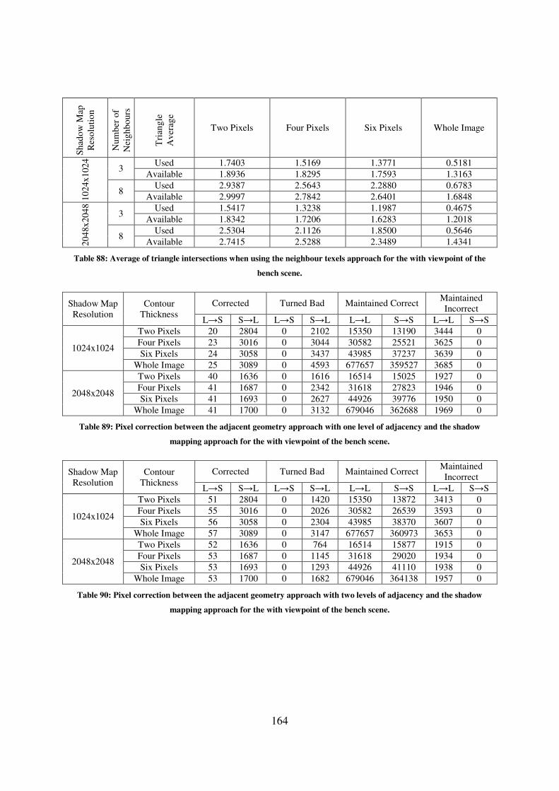
164
Sh
ado
w M
ap
Res
olu
tio
n
Nu
mb
er o
f
Nei
gh
bo
urs
Tri
ang
le
Av
erag
e
Two Pixels Four Pixels Six Pixels Whole Image
10
24x
102
4
3 Used 1.7403 1.5169 1.3771 0.5181
Available 1.8936 1.8295 1.7593 1.3163
8 Used 2.9387 2.5643 2.2880 0.6783
Available 2.9997 2.7842 2.6401 1.6848
20
48x
204
8
3 Used 1.5417 1.3238 1.1987 0.4675
Available 1.8342 1.7206 1.6283 1.2018
8 Used 2.5304 2.1126 1.8500 0.5646
Available 2.7415 2.5288 2.3489 1.4341
Table 88: Average of triangle intersections when using the neighbour texels approach for the with viewpoint of the
bench scene.
Shadow Map
Resolution
Contour
Thickness
Corrected Turned Bad Maintained Correct Maintained
Incorrect
L→S S→L L→S S→L L→L S→S L→L S→S
1024x1024
Two Pixels 20 2804 0 2102 15350 13190 3444 0
Four Pixels 23 3016 0 3044 30582 25521 3625 0
Six Pixels 24 3058 0 3437 43985 37237 3639 0
Whole Image 25 3089 0 4593 677657 359527 3685 0
2048x2048
Two Pixels 40 1636 0 1616 16514 15025 1927 0
Four Pixels 41 1687 0 2342 31618 27823 1946 0
Six Pixels 41 1693 0 2627 44926 39776 1950 0
Whole Image 41 1700 0 3132 679046 362688 1969 0
Table 89: Pixel correction between the adjacent geometry approach with one level of adjacency and the shadow
mapping approach for the with viewpoint of the bench scene.
Shadow Map
Resolution
Contour
Thickness
Corrected Turned Bad Maintained Correct Maintained
Incorrect
L→S S→L L→S S→L L→L S→S L→L S→S
1024x1024
Two Pixels 51 2804 0 1420 15350 13872 3413 0
Four Pixels 55 3016 0 2026 30582 26539 3593 0
Six Pixels 56 3058 0 2304 43985 38370 3607 0
Whole Image 57 3089 0 3147 677657 360973 3653 0
2048x2048
Two Pixels 52 1636 0 764 16514 15877 1915 0
Four Pixels 53 1687 0 1145 31618 29020 1934 0
Six Pixels 53 1693 0 1293 44926 41110 1938 0
Whole Image 53 1700 0 1682 679046 364138 1957 0
Table 90: Pixel correction between the adjacent geometry approach with two levels of adjacency and the shadow
mapping approach for the with viewpoint of the bench scene.

165
Sh
ado
w M
ap
Res
olu
tio
n
Ad
jace
ncy
Lev
el
Tri
ang
le
Av
erag
e
Two Pixels Four Pixels Six Pixels Whole Image
10
24x
102
4
One
Level
Used 2.6226 2.5888 2.5643 1.5079
Available 3.8788 3.8798 3.8819 3.9437
Two
Levels
Used 8.3600 8.2441 8.1693 5.2342
Available 12.3645 12.3552 12.3670 13.6896
20
48x
204
8
One
Level
Used 2.6600 2.6235 2.5947 1.5098
Available 3.8605 3.8669 3.8715 3.9412
Two
Levels
Used 8.4322 8.3126 8.2318 5.2390
Available 12.2375 12.2524 12.2826 13.6755
Table 91: Average of triangle intersections when using the adjacent geometry approach for the with viewpoint of the
bench scene.

166
Contour Thickness Two Pixels Four Pixels Six Pixels Whole Image
Lighting L→S S→L L→S S→L L→S S→L L→S S→L
Sh
ado
w M
ap R
eso
luti
on
10
24x
102
4
Corrected by
Both 7 2804 9 3016 9 3058 10 3089
Turned Bad
by Both 0 1137 0 1602 0 1780 0 1846
Corrected by
Neighbour
Texels Only
2167 0 2255 0 2260 0 2290 0
Corrected by
Adjacent
Geometry
Only
44 0 46 0 47 0 47 0
Turned Bad
by
Neighbour
Texels Only
0 871 0 1261 0 1361 0 1545
Turned Bad
by Adjacent
Geometry
Only
0 283 0 424 0 524 0 1301
20
48x
204
8
Corrected by
Both 39 1636 40 1687 40 1693 40 1700
Turned Bad
by Both 0 533 0 804 0 894 0 916
Corrected by
Neighbour
Texels Only
1283 0 1285 0 1285 0 1302 0
Corrected by
Adjacent
Geometry
Only
13 0 13 0 13 0 13 0
Turned Bad
by
Neighbour
Texels Only
0 932 0 1294 0 1425 0 1479
Turned Bad
by Adjacent
Geometry
Only
0 231 0 341 0 399 0 766
Table 92: Pixel correction by the neighbour texels (9 texels) and the adjacent geometry (2 levels) approaches
separated by lighting change for the with viewpoint of the bench scene.

167
Alg
ori
thm
Ste
p
Confirmations
and Errors
1024x1024 2048x2048
Two Pixels Four Pixels Six Pixel Two Pixels Four Pixels Six Pixel
Sh
ado
w M
ap
Total Contour
Pixels 36910 65811 91380 96758 65457 91013
Correct Light
Pixels
15350
(81.59%)
30582
(89.34%)
43985
(92.31%)
16514
(89.36%)
31618
(94.09%)
44926
(95.76%)
Correct Shadow
Pixels
15292
(84.50%)
28565
(90.45%)
40674
(93.01%)
16641
(91.05%)
30165
(94.70%)
42403
(96.16%)
Incorrect Light
Pixels
3464
(18.41%)
3648
(10.66%)
3663
(7.69%)
1967
(10.64%)
1987
(5.91%)
1991
(4.24%)
Incorrect Shadow
Pixels
2804
(15.50%)
3016
(9.55%)
3058
(6.99%)
1636
(8.95%)
1687
(5.30%)
1693
(3.84%)
Tex
el C
oh
eren
ce
Confirmations in
Light
7381
(39.23%)
20741
(60.59%)
33681
(70.69%)
11032
(59.69%)
25827
(76.85%)
39120
(83.38%)
Confirmations in
Shadow
6585
(36.39%)
17755
(56.22%)
29414
(67.26%)
10280
(56.25%)
23227
(72.92%)
35399
(80.28%)
Wrong
Confirmations in
Light
390
(2.07%)
438
(1.28%)
449
(0.94%)
104
(0.56%)
122
(0.36%)
126
(0.27%)
Wrong
Confirmations in
Shadow
43 (0.24%) 111
(0.35%)
140
(0.32%) 31 (0.17%) 74 (0.23%) 78 (0.18%)
Nei
gh
bo
uri
ng
Tex
els
Corrections from
Light
2148
(11.42%)
2233
(6.52%)
2237
(4.69%)
1311
(7.09%)
1311
(3.90%)
1311
(2.79%)
Confirmations in
Shadow
13900
(76.81%)
26902
(85.18%)
39021
(89.23%)
15726
(86.05%)
29138
(91.48%)
41358
(93.79%)
Ad
jace
nt
Geo
met
ry
Confirmations in
Shadow
14553
(80.42%)
27724
(87.79%)
39854
(91.13%)
16328
(89.34%)
29842
(93.69%)
42082
(95.44%)
Fin
al L
igh
tin
g Wrong
Confirmations in
Light
929
(7.01%)
980
(4.14%)
980
(3.00%)
565
(3.62%)
567
(2.05%)
567
(1.48%)
Wrong
Confirmations in
Shadow
782
(4.56%)
952
(3.37%)
960
(2.52%)
344
(2.05%)
397
(1.48%)
399
(1.08%)
Table 93: Algorithm results of the with viewpoint of the bench scene.
Following below are the results of the “against” viewpoint of the “bench” scene.
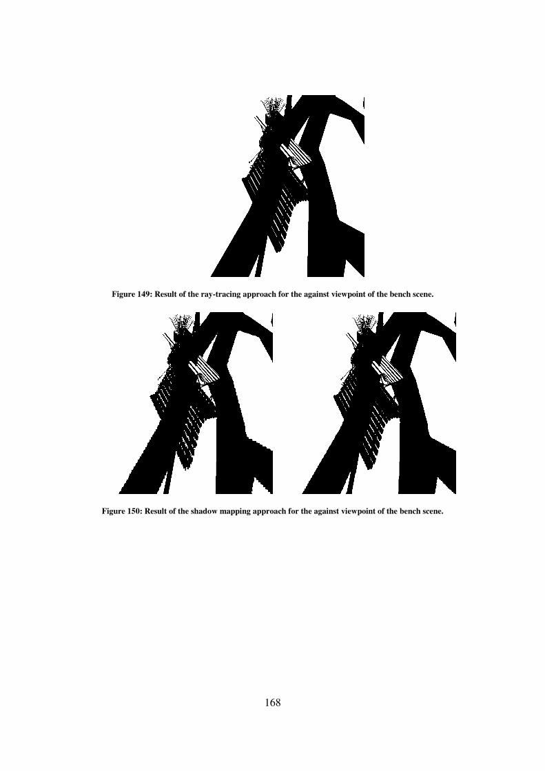
Figure 149: Result of the
Figure 150: Result of the shadow mapping approach for the
168
: Result of the ray-tracing approach for the against viewpoint of the bench scene.
: Result of the shadow mapping approach for the against viewpoint of the
tracing approach for the against viewpoint of the bench scene.
viewpoint of the bench scene.
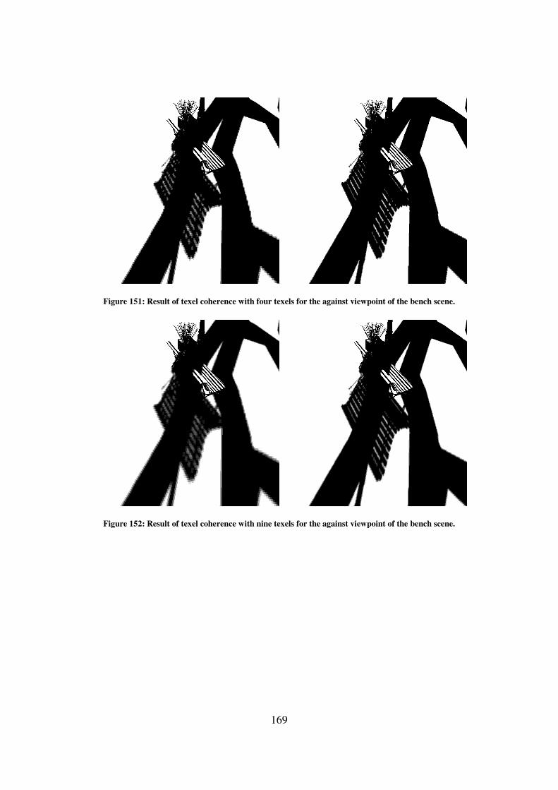
Figure 151: Result of texel coherence with four texels for
Figure 152: Result of texel coherence with nine texels for
169
: Result of texel coherence with four texels for the against viewpoint of the bench scene
: Result of texel coherence with nine texels for the against viewpoint of the bench scene
the against viewpoint of the bench scene.
the against viewpoint of the bench scene.
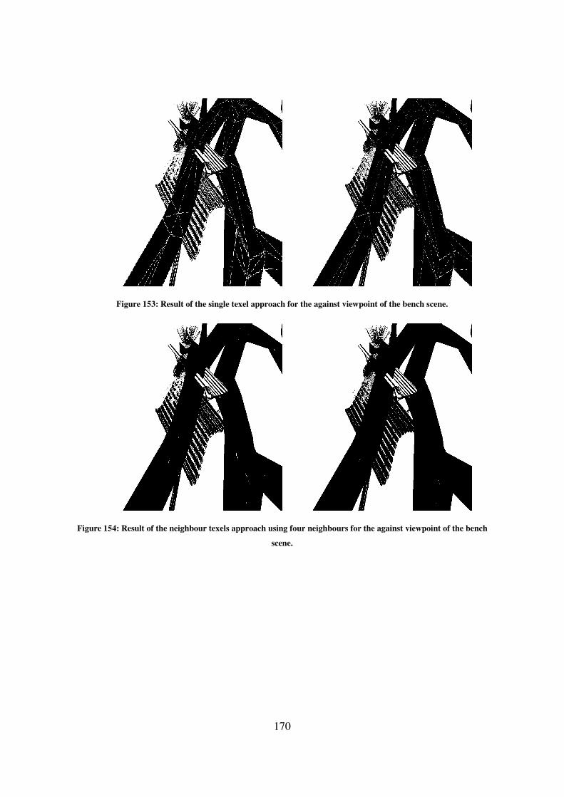
170
Figure 153: Result of the single texel approach for the against viewpoint of the bench scene.
Figure 154: Result of the neighbour texels approach using four neighbours for the against viewpoint of the bench
scene.
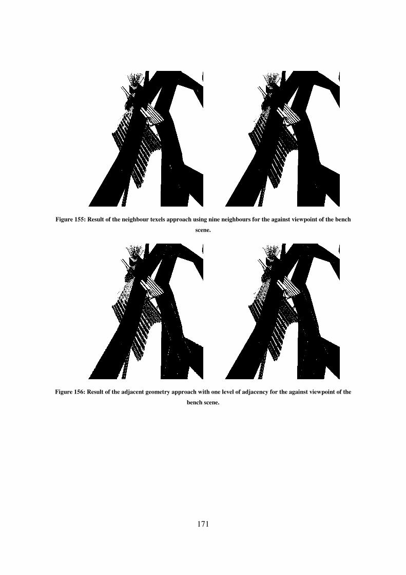
171
Figure 155: Result of the neighbour texels approach using nine neighbours for the against viewpoint of the bench
scene.
Figure 156: Result of the adjacent geometry approach with one level of adjacency for the against viewpoint of the
bench scene.
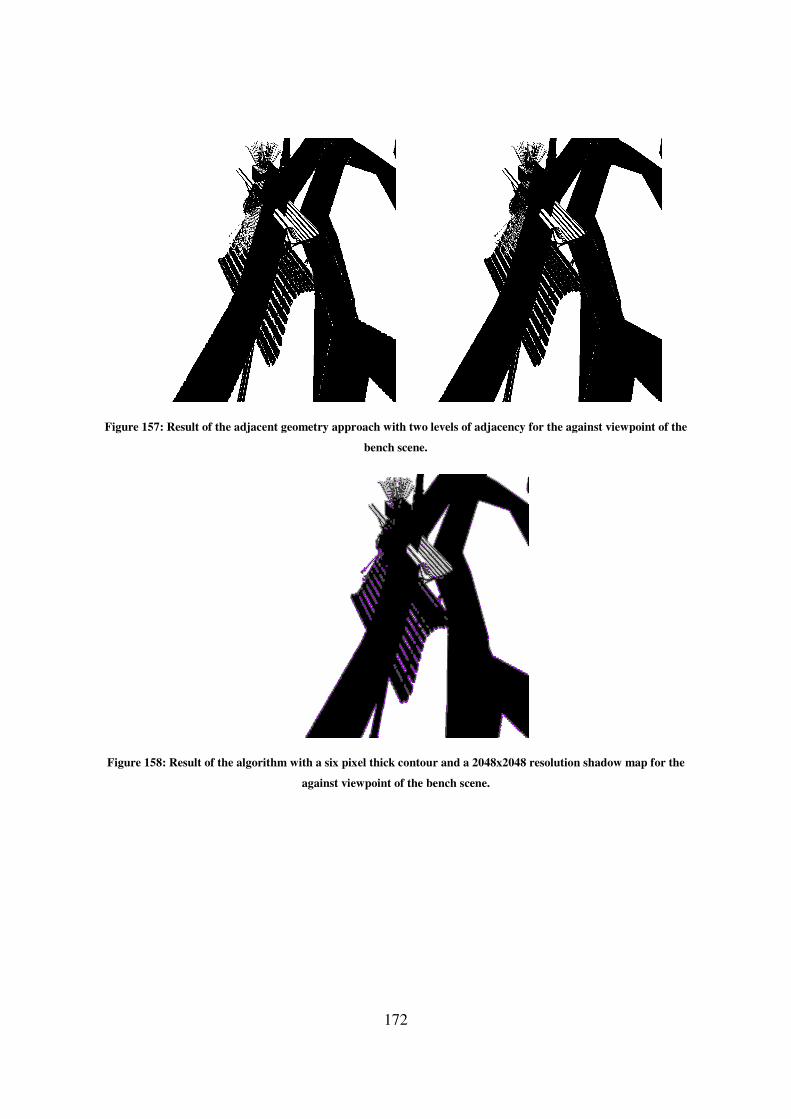
Figure 157: Result of the adjacent geometry
Figure 158: Result of the algorithm
172
adjacent geometry approach with two levels of adjacency for the against viewpoint of the
bench scene.
: Result of the algorithm with a six pixel thick contour and a 2048x2048 resolution shadow map for the
against viewpoint of the bench scene.
the against viewpoint of the
with a six pixel thick contour and a 2048x2048 resolution shadow map for the
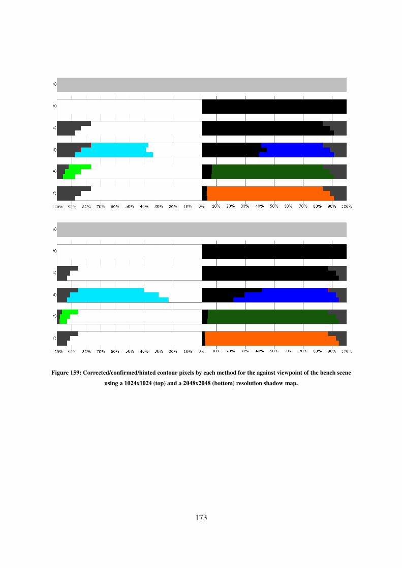
173
Figure 159: Corrected/confirmed/hinted contour pixels by each method for the against viewpoint of the bench scene
using a 1024x1024 (top) and a 2048x2048 (bottom) resolution shadow map.
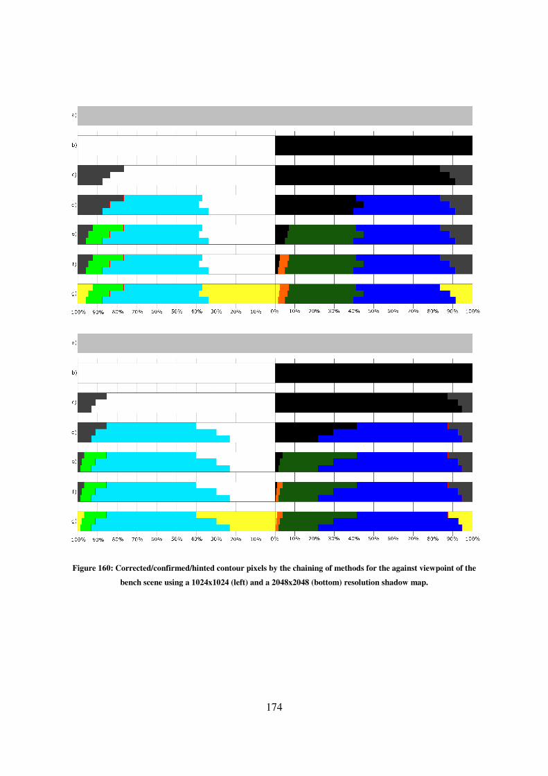
174
Figure 160: Corrected/confirmed/hinted contour pixels by the chaining of methods for the against viewpoint of the
bench scene using a 1024x1024 (left) and a 2048x2048 (bottom) resolution shadow map.

175
Shadow Map
Resolution Approach
Contour Thickness
Two Pixels Four Pixels Six Pixels Whole Image
1024x1024
Pixels in
Contour 36248 64370 86929 1048576
Shadow Map 7171 (19.78%) 8887 (13.81%) 9130 (10.50%) 9542 (0.91%)
Single Texel 6661 (18.38%) 10005 (15.54%) 12383 (14.24%) 40722 (3.88%)
Neighbour
Texels (4
Neighbours)
3390 (9.35%) 5246 (8.15%) 6496 (7.47%) 14574 (1.39%)
Neighbour
Texels (9
Neighbours)
2731 (7.53%) 4048 (6.29%) 4859 (5.59%) 10272 (0.98%)
Adjacent
Geometry (One
Level)
5480 (15.12%) 7526 (11.69%) 8816 (10.14%) 19608 (1.87%)
Adjacent
Geometry
(Two Level)
4708 (12.99%) 6107 (9.49%) 6803 (7.83%) 13372 (1.28%)
2048x2048
Pixels in
Contour 37821 65950 88864 1048576
Shadow Map 5113 (13.52%) 5315 (8.06%) 5338 (6.01%) 5392 (0.51%)
Single Texel 4881 (12.91%) 7234 (10.97%) 9191 (10.34%) 25404 (2.42%)
Neighbour
Texels (4
Neighbours)
1969 (5.21%) 2880 (4.37%) 3470 (3.90%) 7371 (0.70%)
Neighbour
Texels (9
Neighbours)
1465 (3.87%) 2097 (3.18%) 2494 (2.81%) 5022 (0.48%)
Adjacent
Geometry (One
Level)
3648 (9.65%) 4722 (7.16%) 5560 (6.26%) 11058 (1.05%)
Adjacent
Geometry
(Two Level)
3015 (7.97%) 3486 (5.29%) 3872 (4.36%) 6987 (0.67%)
Table 94: Difference between the approaches that use ray-tracing and the actual ray-tracer for the against viewpoint
of the bench scene.
Shadow Map Resolution Contour Thickness
Two Pixels Four Pixels Six Pixels
1024x1024 7171 of 9542 (75.15%) 8887 of 9542 (93.14%) 9130 of 9542 (95.68%)
2048x2048 5113 of 5392 (94.83%) 5315 of 5392 (98.57%) 5338 of 5392 (99.00%)
Table 95: Wrongly defined pixels in the shadow mapping result which are inside the contour in the against viewpoint
of the bench scene.

176
Shadow Map Resolution Contour Thickness Pixel Shading
Light Shadow
1024x1024
Two Pixels 4063 of 17429 3108 of 18819
Four Pixels 4966 of 30268 3921 of 34102
Six Pixels 5037 of 40012 4093 of 46917
Whole Image 5080 of 604815 4462 of 443761
2048x2048
Two Pixels 2647 of 18100 2466 of 19721
Four Pixels 2719 of 30480 2596 of 35470
Six Pixels 2720 of 39980 2618 of 48884
Whole Image 2745 of 604295 2647 of 444281
Table 96: Pixels that the shadow map defines wrongly in the against viewpoint of the bench scene, separated in pixels
defined in light and in shadow, compared to the total amount of pixels lighted in the same way.
Shadow
Map
Resolution
Contour
Thickness
Texel Coherence
Light Shadow
Confirmed Incorrectly
Confirmed Undecided Confirmed
Incorrectly
Confirmed Undecided
1024x1024
Two Pixels 6944
(39.84%) 50 (0.29%)
10485
(60.16%)
7988
(42.45%) 7 (0.04%)
10831
(57.55%)
Four Pixels 13631
(45.03%) 65 (0.21%)
16637
(54.97%)
14920
(43.75%) 30 (0.09%)
19182
(56.25%)
Six Pixels 21521
(53.79%) 79 (0.20%)
18491
(46.21%)
24345
(51.89%)
102
(0.22%)
22572
(48.11%)
Whole
Image
585401
(96.79%) 85 (0.01%)
19414
(3.21%)
419750
(94.59%)
425
(0.10%)
24011
(5.41%)
2048x2048
Two Pixels 8223
(45.43%) 43 (0.24%)
9877
(54.57%)
9084
(46.06%) 19 (0.10%)
10637
(53.94%)
Four Pixels 18729
(61.45%) 52 (0.17%)
11751
(38.55%)
22499
(63.43%) 79 (0.22%)
12971
(36.57%)
Six Pixels 28097
(70.28%) 53 (0.13%)
11883
(29.72%)
35753
(73.14%) 99 (0.20%)
13131
(26.86%)
Whole
Image
592322
(98.02%) 53 (0.01%)
11973
(1.98%)
431064
(97.03%)
115
(0.03%)
13217
(2.97%)
Table 97: Pixel confirmation when using texel coherence with four texels for the against viewpoint of the bench scene.
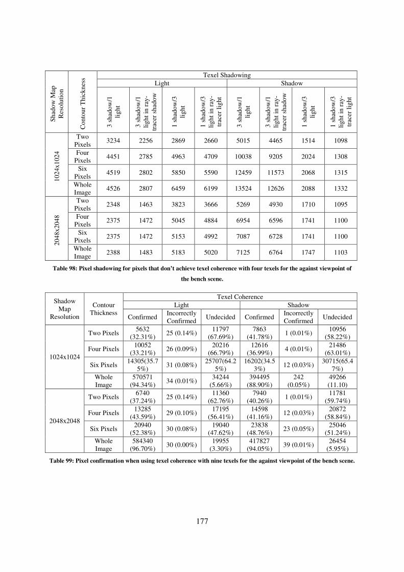
177
Sh
ado
w M
ap
Res
olu
tio
n
Co
nto
ur
Th
ick
nes
s Texel Shadowing
Light Shadow
3 s
had
ow
/1
lig
ht
3 s
had
ow
/1
lig
ht
in r
ay-
trac
er s
had
ow
1 s
had
ow
/3
lig
ht
1 s
had
ow
/3
lig
ht
in r
ay-
trac
er l
igh
t
3 s
had
ow
/1
lig
ht
3 s
had
ow
/1
lig
ht
in r
ay-
trac
er s
had
ow
1 s
had
ow
/3
lig
ht
1 s
had
ow
/3
lig
ht
in r
ay-
trac
er l
igh
t
10
24x
102
4
Two
Pixels 3234 2256 2869 2660 5015 4465 1514 1098
Four
Pixels 4451 2785 4963 4709 10038 9205 2024 1308
Six
Pixels 4519 2802 5850 5590 12459 11573 2068 1315
Whole
Image 4526 2807 6459 6199 13524 12626 2088 1332
20
48x
204
8
Two
Pixels 2348 1463 3823 3666 5269 4930 1710 1095
Four
Pixels 2375 1472 5045 4884 6954 6596 1741 1100
Six
Pixels 2375 1472 5153 4992 7087 6728 1741 1100
Whole
Image 2388 1483 5183 5020 7125 6764 1747 1103
Table 98: Pixel shadowing for pixels that don’t achieve texel coherence with four texels for the against viewpoint of
the bench scene.
Shadow
Map
Resolution
Contour
Thickness
Texel Coherence
Light Shadow
Confirmed Incorrectly
Confirmed Undecided Confirmed
Incorrectly
Confirmed Undecided
1024x1024
Two Pixels 5632
(32.31%) 25 (0.14%)
11797
(67.69%)
7863
(41.78%) 1 (0.01%)
10956
(58.22%)
Four Pixels 10052
(33.21%) 26 (0.09%)
20216
(66.79%)
12616
(36.99%) 4 (0.01%)
21486
(63.01%)
Six Pixels 14305(35.7
5%) 31 (0.08%)
25707(64.2
5%)
16202(34.5
3%) 12 (0.03%)
30715(65.4
7%)
Whole
Image
570571
(94.34%) 34 (0.01%)
34244
(5.66%)
394495
(88.90%)
242
(0.05%)
49266
(11.10)
2048x2048
Two Pixels 6740
(37.24%) 25 (0.14%)
11360
(62.76%)
7940
(40.26%) 1 (0.01%)
11781
(59.74%)
Four Pixels 13285
(43.59%) 29 (0.10%)
17195
(56.41%)
14598
(41.16%) 12 (0.03%)
20872
(58.84%)
Six Pixels 20940
(52.38%) 30 (0.08%)
19040
(47.62%)
23838
(48.76%) 23 (0.05%)
25046
(51.24%)
Whole
Image
584340
(96.70%) 30 (0.00%)
19955
(3.30%)
417827
(94.05%) 39 (0.01%)
26454
(5.95%)
Table 99: Pixel confirmation when using texel coherence with nine texels for the against viewpoint of the bench scene.
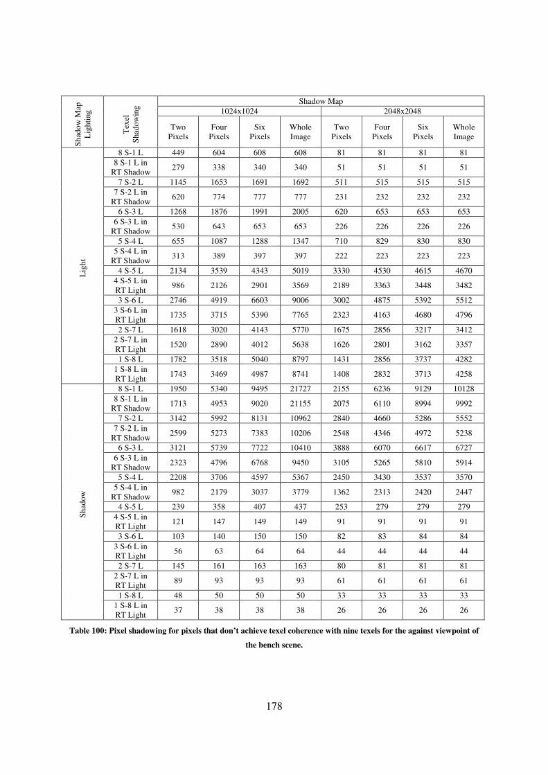
178
Sh
ado
w M
ap
Lig
hti
ng
Tex
el
Sh
ado
win
g Shadow Map
1024x1024 2048x2048
Two
Pixels
Four
Pixels
Six
Pixels
Whole
Image
Two
Pixels
Four
Pixels
Six
Pixels
Whole
Image
Lig
ht
8 S-1 L 449 604 608 608 81 81 81 81
8 S-1 L in
RT Shadow 279 338 340 340 51 51 51 51
7 S-2 L 1145 1653 1691 1692 511 515 515 515
7 S-2 L in
RT Shadow 620 774 777 777 231 232 232 232
6 S-3 L 1268 1876 1991 2005 620 653 653 653
6 S-3 L in
RT Shadow 530 643 653 653 226 226 226 226
5 S-4 L 655 1087 1288 1347 710 829 830 830
5 S-4 L in
RT Shadow 313 389 397 397 222 223 223 223
4 S-5 L 2134 3539 4343 5019 3330 4530 4615 4670
4 S-5 L in
RT Light 986 2126 2901 3569 2189 3363 3448 3482
3 S-6 L 2746 4919 6603 9006 3002 4875 5392 5512
3 S-6 L in
RT Light 1735 3715 5390 7765 2323 4163 4680 4796
2 S-7 L 1618 3020 4143 5770 1675 2856 3217 3412
2 S-7 L in
RT Light 1520 2890 4012 5638 1626 2801 3162 3357
1 S-8 L 1782 3518 5040 8797 1431 2856 3737 4282
1 S-8 L in
RT Light 1743 3469 4987 8741 1408 2832 3713 4258
Sh
ado
w
8 S-1 L 1950 5340 9495 21727 2155 6236 9129 10128
8 S-1 L in
RT Shadow 1713 4953 9020 21155 2075 6110 8994 9992
7 S-2 L 3142 5992 8131 10962 2840 4660 5286 5552
7 S-2 L in
RT Shadow 2599 5273 7383 10206 2548 4346 4972 5238
6 S-3 L 3121 5739 7722 10410 3888 6070 6617 6727
6 S-3 L in
RT Shadow 2323 4796 6768 9450 3105 5265 5810 5914
5 S-4 L 2208 3706 4597 5367 2450 3430 3537 3570
5 S-4 L in
RT Shadow 982 2179 3037 3779 1362 2313 2420 2447
4 S-5 L 239 358 407 437 253 279 279 279
4 S-5 L in
RT Light 121 147 149 149 91 91 91 91
3 S-6 L 103 140 150 150 82 83 84 84
3 S-6 L in
RT Light 56 63 64 64 44 44 44 44
2 S-7 L 145 161 163 163 80 81 81 81
2 S-7 L in
RT Light 89 93 93 93 61 61 61 61
1 S-8 L 48 50 50 50 33 33 33 33
1 S-8 L in
RT Light 37 38 38 38 26 26 26 26
Table 100: Pixel shadowing for pixels that don’t achieve texel coherence with nine texels for the against viewpoint of
the bench scene.
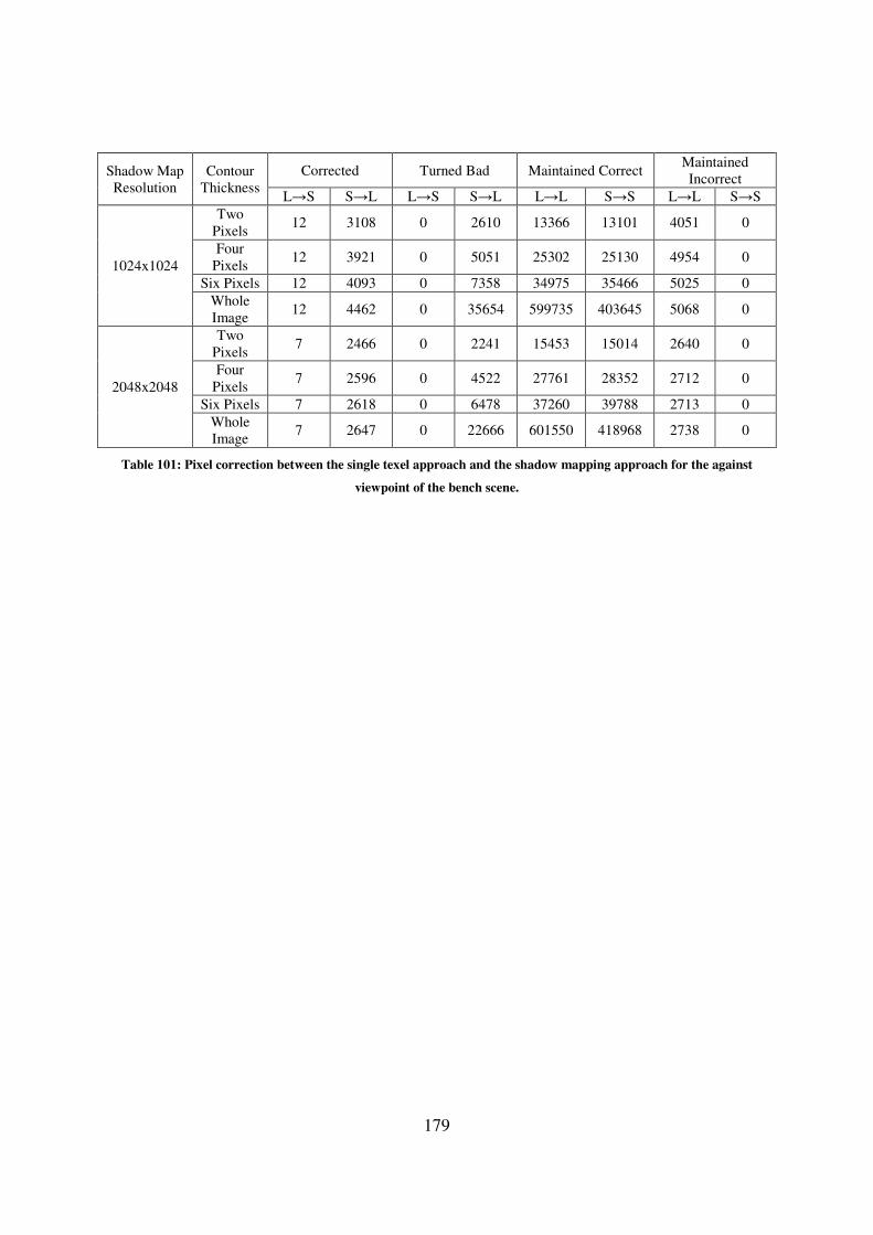
179
Shadow Map
Resolution
Contour
Thickness
Corrected Turned Bad Maintained Correct Maintained
Incorrect
L→S S→L L→S S→L L→L S→S L→L S→S
1024x1024
Two
Pixels 12 3108 0 2610 13366 13101 4051 0
Four
Pixels 12 3921 0 5051 25302 25130 4954 0
Six Pixels 12 4093 0 7358 34975 35466 5025 0
Whole
Image 12 4462 0 35654 599735 403645 5068 0
2048x2048
Two
Pixels 7 2466 0 2241 15453 15014 2640 0
Four
Pixels 7 2596 0 4522 27761 28352 2712 0
Six Pixels 7 2618 0 6478 37260 39788 2713 0
Whole
Image 7 2647 0 22666 601550 418968 2738 0
Table 101: Pixel correction between the single texel approach and the shadow mapping approach for the against
viewpoint of the bench scene.
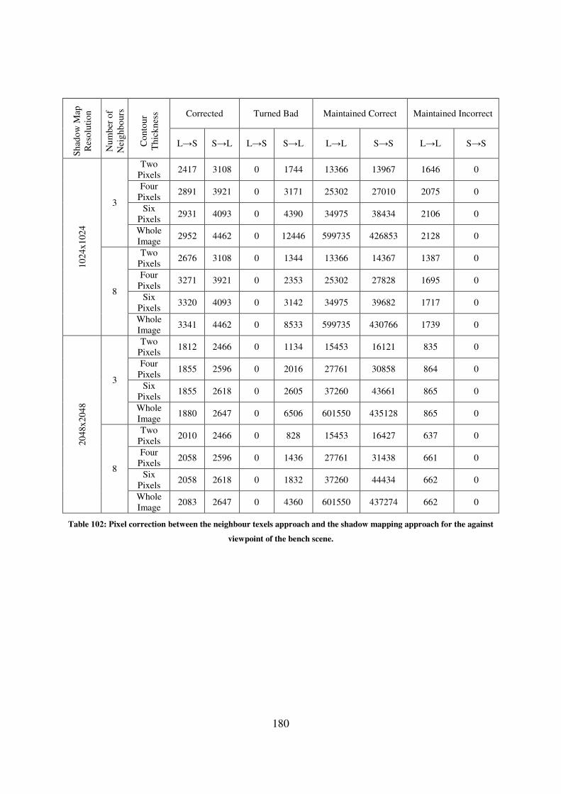
180
Sh
ado
w M
ap
Res
olu
tio
n
Nu
mb
er o
f
Nei
gh
bo
urs
Co
nto
ur
Th
ick
nes
s Corrected Turned Bad Maintained Correct Maintained Incorrect
L→S S→L L→S S→L L→L S→S L→L S→S
10
24x
102
4
3
Two
Pixels 2417 3108 0 1744 13366 13967 1646 0
Four
Pixels 2891 3921 0 3171 25302 27010 2075 0
Six
Pixels 2931 4093 0 4390 34975 38434 2106 0
Whole
Image 2952 4462 0 12446 599735 426853 2128 0
8
Two
Pixels 2676 3108 0 1344 13366 14367 1387 0
Four
Pixels 3271 3921 0 2353 25302 27828 1695 0
Six
Pixels 3320 4093 0 3142 34975 39682 1717 0
Whole
Image 3341 4462 0 8533 599735 430766 1739 0
20
48x
204
8
3
Two
Pixels 1812 2466 0 1134 15453 16121 835 0
Four
Pixels 1855 2596 0 2016 27761 30858 864 0
Six
Pixels 1855 2618 0 2605 37260 43661 865 0
Whole
Image 1880 2647 0 6506 601550 435128 865 0
8
Two
Pixels 2010 2466 0 828 15453 16427 637 0
Four
Pixels 2058 2596 0 1436 27761 31438 661 0
Six
Pixels 2058 2618 0 1832 37260 44434 662 0
Whole
Image 2083 2647 0 4360 601550 437274 662 0
Table 102: Pixel correction between the neighbour texels approach and the shadow mapping approach for the against
viewpoint of the bench scene.
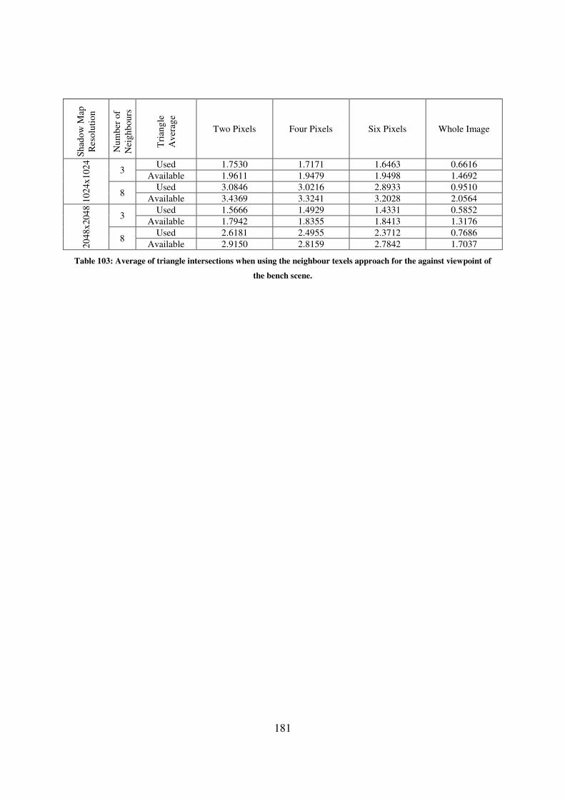
181
Sh
ado
w M
ap
Res
olu
tio
n
Nu
mb
er o
f
Nei
gh
bo
urs
Tri
ang
le
Av
erag
e
Two Pixels Four Pixels Six Pixels Whole Image
10
24x
102
4
3 Used 1.7530 1.7171 1.6463 0.6616
Available 1.9611 1.9479 1.9498 1.4692
8 Used 3.0846 3.0216 2.8933 0.9510
Available 3.4369 3.3241 3.2028 2.0564
20
48x
204
8
3 Used 1.5666 1.4929 1.4331 0.5852
Available 1.7942 1.8355 1.8413 1.3176
8 Used 2.6181 2.4955 2.3712 0.7686
Available 2.9150 2.8159 2.7842 1.7037
Table 103: Average of triangle intersections when using the neighbour texels approach for the against viewpoint of
the bench scene.
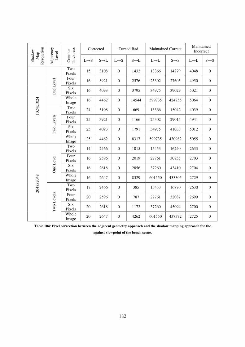
182
Sh
ado
w
Map
Res
olu
tio
n
Ad
jace
ncy
Lev
el
Co
nto
ur
Th
ick
nes
s Corrected Turned Bad Maintained Correct Maintained
Incorrect
L→S S→L L→S S→L L→L S→S L→L S→S
10
24x
102
4 O
ne
Lev
el
Two
Pixels 15 3108 0 1432 13366 14279 4048 0
Four
Pixels 16 3921 0 2576 25302 27605 4950 0
Six
Pixels 16 4093 0 3795 34975 39029 5021 0
Whole
Image 16 4462 0 14544 599735 424755 5064 0
Tw
o L
evel
s
Two
Pixels 24 3108 0 669 13366 15042 4039 0
Four
Pixels 25 3921 0 1166 25302 29015 4941 0
Six
Pixels 25 4093 0 1791 34975 41033 5012 0
Whole
Image 25 4462 0 8317 599735 430982 5055 0
20
48x
204
8 O
ne
Lev
el
Two
Pixels 14 2466 0 1015 15453 16240 2633 0
Four
Pixels 16 2596 0 2019 27761 30855 2703 0
Six
Pixels 16 2618 0 2856 37260 43410 2704 0
Whole
Image 16 2647 0 8329 601550 433305 2729 0
Tw
o L
evel
s
Two
Pixels 17 2466 0 385 15453 16870 2630 0
Four
Pixels 20 2596 0 787 27761 32087 2699 0
Six
Pixels 20 2618 0 1172 37260 45094 2700 0
Whole
Image 20 2647 0 4262 601550 437372 2725 0
Table 104: Pixel correction between the adjacent geometry approach and the shadow mapping approach for the
against viewpoint of the bench scene.
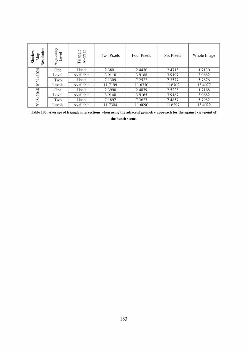
183
Sh
ado
w
Map
Res
olu
tio
n
Ad
jace
ncy
Lev
el
Tri
ang
le
Av
erag
e
Two Pixels Four Pixels Six Pixels Whole Image
10
24x
102
4
One
Level
Used 2.3801 2.4430 2.4713 1.7130
Available 3.9118 3.9188 3.9197 3.9682
Two
Levels
Used 7.1309 7.2522 7.3577 5.7876
Available 11.7199 11.6330 11.6702 13.4077
20
48x
204
8
One
Level
Used 2.3990 2.4839 2.5223 1.7168
Available 3.9140 3.9165 3.9187 3.9682
Two
Levels
Used 7.1897 7.3627 7.4857 5.7982
Available 11.7304 11.6090 11.6297 13.4022
Table 105: Average of triangle intersections when using the adjacent geometry approach for the against viewpoint of
the bench scene.

184
Contour Thickness Two Pixels Four Pixels Six Pixels Whole Image
Lighting L→S S→L L→S S→L L→S S→L L→S S→L
Sh
ado
w M
ap R
eso
luti
on
10
24x
102
4
Corrected by
Both 12 3108 12 3921 12 4093 12 4462
Turned Bad
by Both 0 477 0 793 0 1143 0 3701
Corrected by
Neighbour
Texels Only
2664 0 3259 0 3308 0 3329 0
Corrected by
Adjacent
Geometry
Only
12 0 13 0 13 0 13 0
Turned Bad
by
Neighbour
Texels Only
0 867 0 1560 0 1999 0 4832
Turned Bad
by Adjacent
Geometry
Only
0 192 0 373 0 648 0 4616
20
48x
204
8
Corrected by
Both 10 2466 11 2596 11 2618 11 2647
Turned Bad
by Both 0 220 0 428 0 566 0 1637
Corrected by
Neighbour
Texels Only
2000 0 2047 0 2047 0 2072 0
Corrected by
Adjacent
Geometry
Only
7 0 9 0 9 0 9 0
Turned Bad
by
Neighbour
Texels Only
0 608 0 1008 0 1266 0 2723
Turned Bad
by Adjacent
Geometry
Only
0 165 0 359 0 606 0 2625
Table 106: Pixel correction by the neighbour texels (9 texels) and the adjacent geometry (2 levels) approaches
separated by lighting change for the against viewpoint of the bench scene.
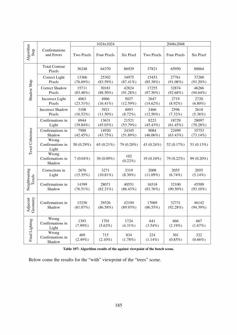
185
Alg
ori
thm
Ste
p
Confirmations
and Errors
1024x1024 2048x2048
Two Pixels Four Pixels Six Pixel Two Pixels Four Pixels Six Pixel
Sh
ado
w M
ap
Total Contour
Pixels 36248 64370 86929 37821 65950 88864
Correct Light
Pixels
13366
(76.69%)
25302
(83.59%)
34975
(87.41%)
15453
(85.38%)
27761
(91.08%)
37260
(93.20%)
Correct Shadow
Pixels
15711
(83.48%)
30181
(88.50%)
42824
(91.28%)
17255
(87.50%)
32874
(92.68%)
46266
(94.64%)
Incorrect Light
Pixels
4063
(23.31%)
4966
(16.41%)
5037
(12.59%)
2647
(14.62%)
2719
(8.92%)
2720
(6.80%)
Incorrect Shadow
Pixels
3108
(16.52%)
3921
(11.50%)
4093
(8.72%)
2466
(12.50%)
2596
(7.32%)
2618
(5.36%)
Tex
el C
oh
eren
ce
Confirmations in
Light
6944
(39.84%)
13631
(45.03%)
21521
(53.79%)
8223
(45.43%)
18729
(61.45%)
28097
(70.28%)
Confirmations in
Shadow
7988
(42.45%)
14920
(43.75%)
24345
(51.89%)
9084
(46.06%)
22499
(63.43%)
35753
(73.14%)
Wrong
Confirmations in
Light
50 (0.29%) 65 (0.21%) 79 (0.20%) 43 (0.24%) 52 (0.17%) 53 (0.13%)
Wrong
Confirmations in
Shadow
7 (0.04%) 30 (0.09%) 102
(0.22%) 19 (0.10%) 79 (0.22%) 99 (0.20%)
Nei
gh
bo
uri
ng
Tex
els
Corrections in
Light
2676
(15.35%)
3271
(10.81%)
3319
(8.30%)
2008
(11.09%)
2055
(6.74%)
2055
(5.14%)
Confirmations in
Shadow
14399
(76.51%)
28071
(82.31%)
40551
(86.43%)
16518
(83.76%)
32100
(90.50%)
45509
(93.10%)
Ad
jace
nt
Geo
met
ry
Confirmations in
Shadow
15256
(81.07%)
29526
(86.58%)
42194
(89.93%)
17069
(86.55%)
32731
(92.28%)
46142
(94.39%)
Fin
al L
igh
tin
g Wrong
Confirmations in
Light
1393
(7.99%)
1701
(5.62%)
1724
(4.31%)
641
(3.54%)
666
(2.19%)
667
(1.67%)
Wrong
Confirmations in
Shadow
469
(2.49%)
715
(2.10%)
834
(1.78%)
224
(1.14%)
301
(0.85%)
322
(0.66%)
Table 107: Algorithm results of the against viewpoint of the bench scene.
Below come the results for the “with” viewpoint of the “trees” scene.
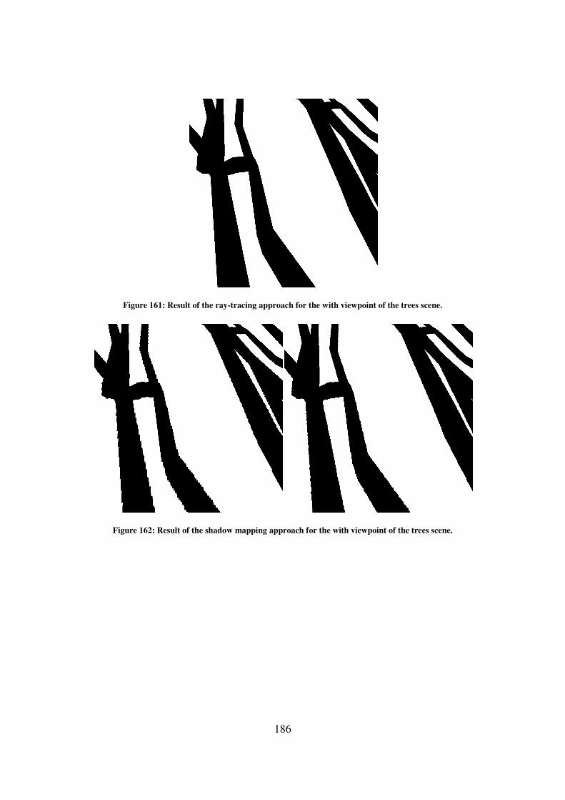
Figure 161: Result of the ray
Figure 162: Result of the shadow mapping approach for the
186
: Result of the ray-tracing approach for the with viewpoint of the trees scene.
: Result of the shadow mapping approach for the with viewpoint of the
tracing approach for the with viewpoint of the trees scene.
viewpoint of the trees scene.
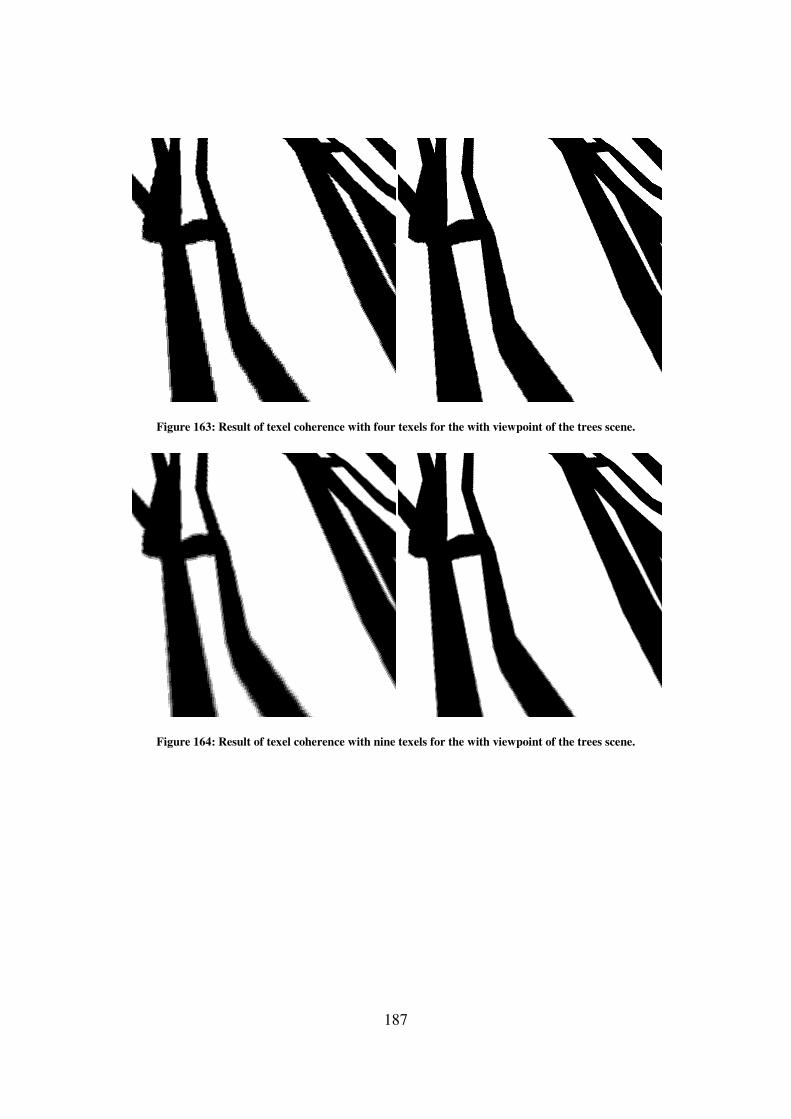
Figure 163: Result of texel coherence with four texels for
Figure 164: Result of texel coherence with nine texels for
187
: Result of texel coherence with four texels for the with viewpoint of the trees scene
: Result of texel coherence with nine texels for the with viewpoint of the trees scene
the with viewpoint of the trees scene.
the with viewpoint of the trees scene.
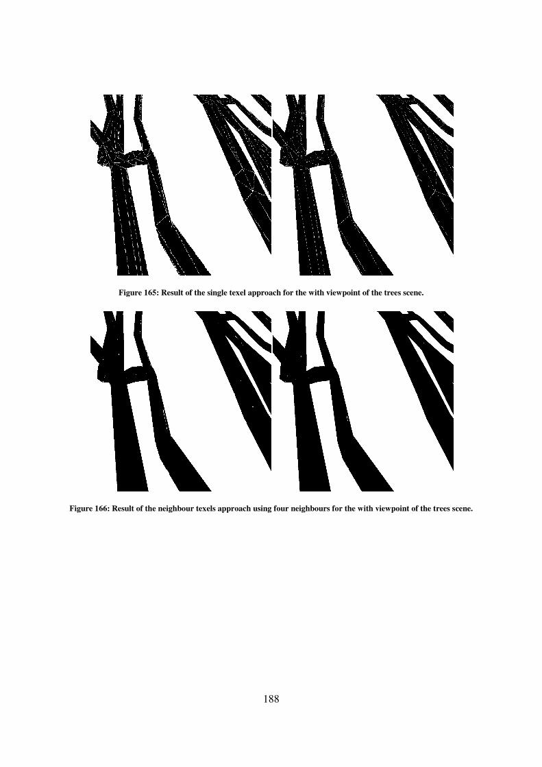
188
Figure 165: Result of the single texel approach for the with viewpoint of the trees scene.
Figure 166: Result of the neighbour texels approach using four neighbours for the with viewpoint of the trees scene.

189
Figure 167: Result of the neighbour texels approach using nine neighbours for the with viewpoint of the trees scene.
Figure 168: Result of the adjacent geometry approach with one level of adjacency for the with viewpoint of the trees
scene.
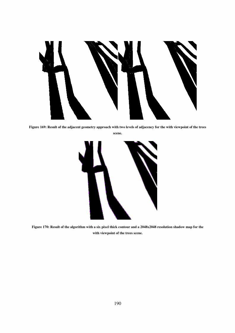
Figure 169: Result of the adjacent geometry
Figure 170: Result of the algorithm with a six pixel thick contour and a 2048x2048 resolution shadow map for the
190
adjacent geometry approach with two levels of adjacency for the with viewpoint of the trees
scene.
: Result of the algorithm with a six pixel thick contour and a 2048x2048 resolution shadow map for the
with viewpoint of the trees scene.
the with viewpoint of the trees
: Result of the algorithm with a six pixel thick contour and a 2048x2048 resolution shadow map for the
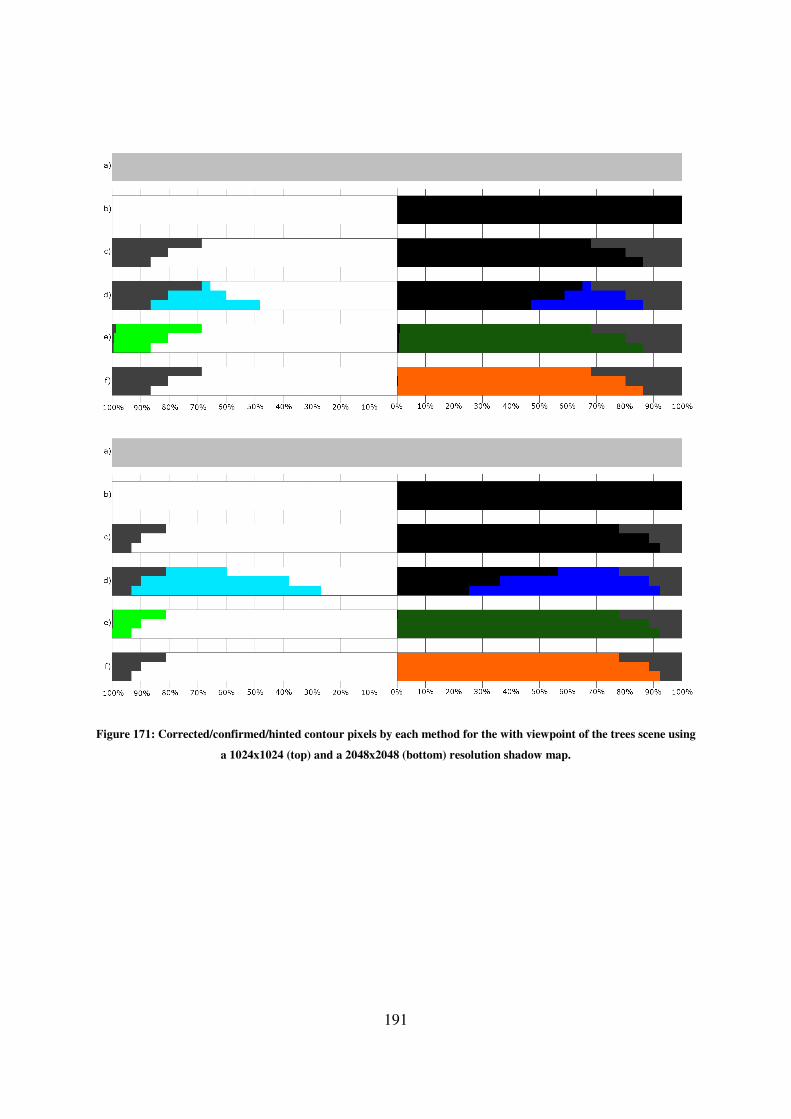
191
Figure 171: Corrected/confirmed/hinted contour pixels by each method for the with viewpoint of the trees scene using
a 1024x1024 (top) and a 2048x2048 (bottom) resolution shadow map.
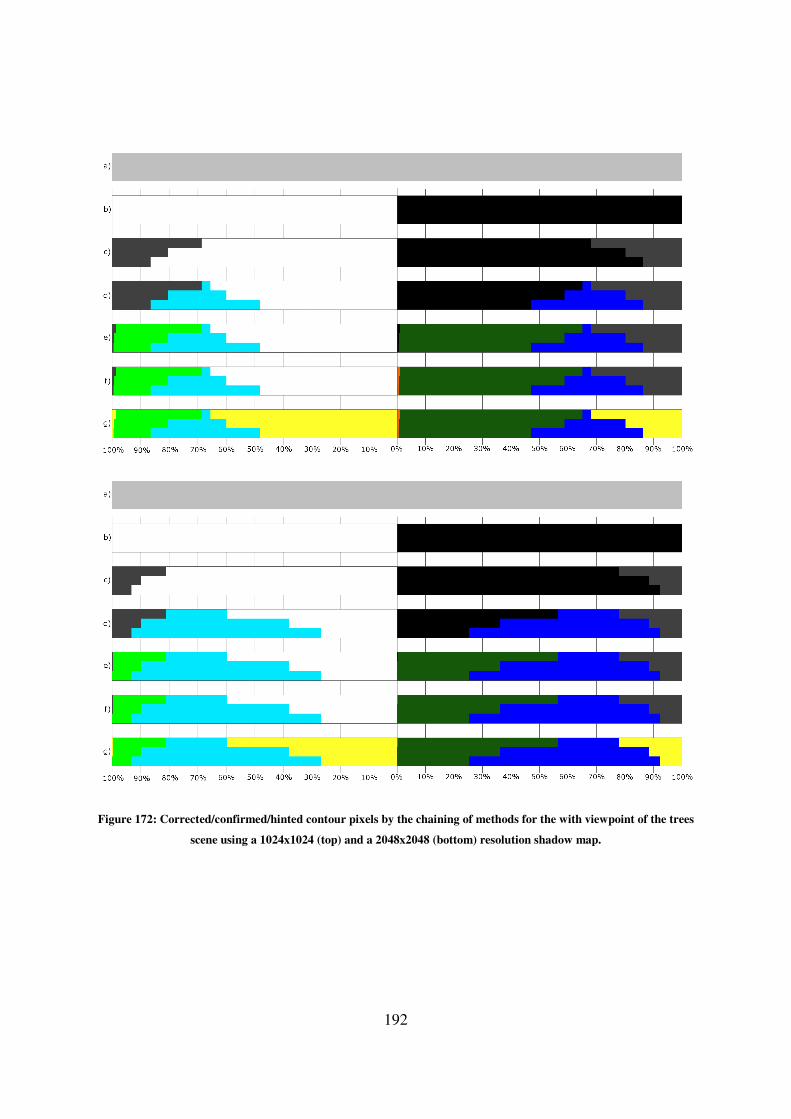
192
Figure 172: Corrected/confirmed/hinted contour pixels by the chaining of methods for the with viewpoint of the trees
scene using a 1024x1024 (top) and a 2048x2048 (bottom) resolution shadow map.
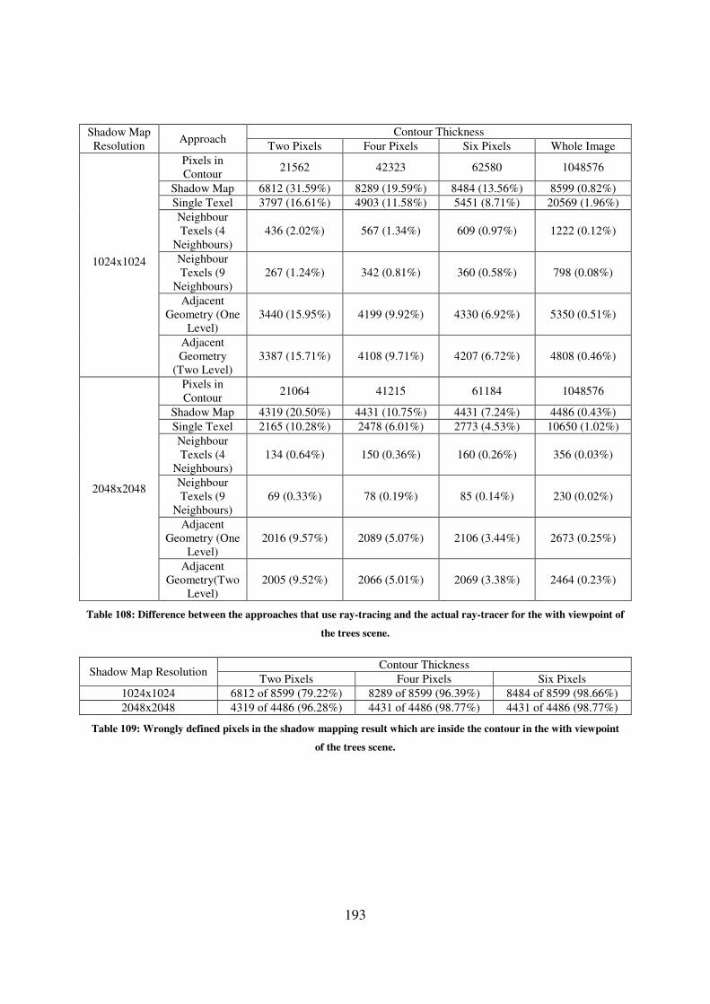
193
Shadow Map
Resolution Approach
Contour Thickness
Two Pixels Four Pixels Six Pixels Whole Image
1024x1024
Pixels in
Contour 21562 42323 62580 1048576
Shadow Map 6812 (31.59%) 8289 (19.59%) 8484 (13.56%) 8599 (0.82%)
Single Texel 3797 (16.61%) 4903 (11.58%) 5451 (8.71%) 20569 (1.96%)
Neighbour
Texels (4
Neighbours)
436 (2.02%) 567 (1.34%) 609 (0.97%) 1222 (0.12%)
Neighbour
Texels (9
Neighbours)
267 (1.24%) 342 (0.81%) 360 (0.58%) 798 (0.08%)
Adjacent
Geometry (One
Level)
3440 (15.95%) 4199 (9.92%) 4330 (6.92%) 5350 (0.51%)
Adjacent
Geometry
(Two Level)
3387 (15.71%) 4108 (9.71%) 4207 (6.72%) 4808 (0.46%)
2048x2048
Pixels in
Contour 21064 41215 61184 1048576
Shadow Map 4319 (20.50%) 4431 (10.75%) 4431 (7.24%) 4486 (0.43%)
Single Texel 2165 (10.28%) 2478 (6.01%) 2773 (4.53%) 10650 (1.02%)
Neighbour
Texels (4
Neighbours)
134 (0.64%) 150 (0.36%) 160 (0.26%) 356 (0.03%)
Neighbour
Texels (9
Neighbours)
69 (0.33%) 78 (0.19%) 85 (0.14%) 230 (0.02%)
Adjacent
Geometry (One
Level)
2016 (9.57%) 2089 (5.07%) 2106 (3.44%) 2673 (0.25%)
Adjacent
Geometry(Two
Level)
2005 (9.52%) 2066 (5.01%) 2069 (3.38%) 2464 (0.23%)
Table 108: Difference between the approaches that use ray-tracing and the actual ray-tracer for the with viewpoint of
the trees scene.
Shadow Map Resolution Contour Thickness
Two Pixels Four Pixels Six Pixels
1024x1024 6812 of 8599 (79.22%) 8289 of 8599 (96.39%) 8484 of 8599 (98.66%)
2048x2048 4319 of 4486 (96.28%) 4431 of 4486 (98.77%) 4431 of 4486 (98.77%)
Table 109: Wrongly defined pixels in the shadow mapping result which are inside the contour in the with viewpoint
of the trees scene.
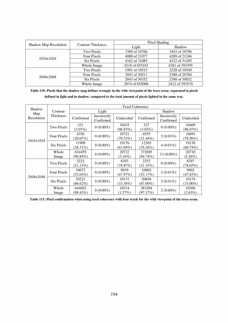
194
Shadow Map Resolution Contour Thickness Pixel Shading
Light Shadow
1024x1024
Two Pixels 3369 of 10766 3443 of 10796
Four Pixels 4080 of 21077 4209 of 21246
Six Pixels 4162 of 31085 4322 of 31495
Whole Image 4218 of 655181 4381 of 393395
2048x2048
Two Pixels 1991 of 10515 2328 of 10549
Four Pixels 2043 of 20511 2388 of 20704
Six Pixels 2043 of 30352 2388 of 30832
Whole Image 2074 of 655006 2412 of 393570
Table 110: Pixels that the shadow map defines wrongly in the with viewpoint of the trees scene, separated in pixels
defined in light and in shadow, compared to the total amount of pixels lighted in the same way.
Shadow
Map
Resolution
Contour
Thickness
Texel Coherence
Light Shadow
Confirmed Incorrectly
Confirmed Undecided Confirmed
Incorrectly
Confirmed Undecided
1024x1024
Two Pixels 331
(3.07%) 0 (0.00%)
10435
(96.93%)
327
(3.03%) 0 (0.00%)
10469
(96.97%)
Four Pixels 4356
(20.67%) 0 (0.00%)
16721
(79.33%)
4555
(21.44%) 2 (0.01%)
16691
(78.56%)
Six Pixels 11909
(38.31%) 0 (0.00%)
19176
(61.69%)
12365
(39.26%) 4 (0.01%)
19130
(60.74%)
Whole
Image
634459
(96.84%) 0 (0.00%)
20722
(3.16%)
372685
(94.74%) 13 (0.00%)
20710
(5.26%)
2048x2048
Two Pixels 2222
(21.13%) 0 (0.00%)
8293
(78.87%)
2252
(21.35%) 0 (0.00%)
8297
(78.65%)
Four Pixels 10672
(52.03%) 0 (0.00%)
9839
(47.97%)
10802
(52.17%) 2 (0.01%)
9902
(47.83%)
Six Pixels 20221
(66.62%) 0 (0.00%)
10131
(33.38%)
20658
(67.00%) 2 (0.01%)
10174
(33.00%)
Whole
Image
644692
(98.43%) 0 (0.00%)
10314
(1.57%)
383204
(97.37%) 2 (0.00%)
10366
(2.63%)
Table 111: Pixel confirmation when using texel coherence with four texels for the with viewpoint of the trees scene.
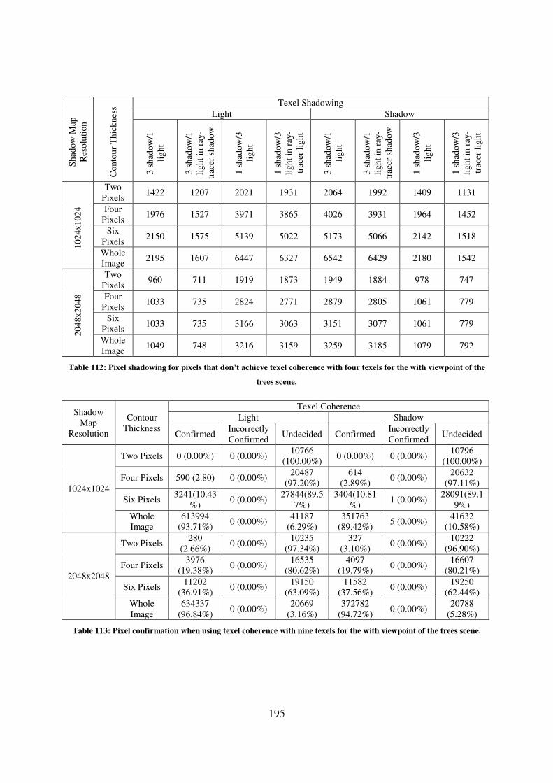
195
Sh
ado
w M
ap
Res
olu
tio
n
Co
nto
ur
Th
ick
nes
s Texel Shadowing
Light Shadow
3 s
had
ow
/1
lig
ht
3 s
had
ow
/1
lig
ht
in r
ay-
trac
er s
had
ow
1 s
had
ow
/3
lig
ht
1 s
had
ow
/3
lig
ht
in r
ay-
trac
er l
igh
t
3 s
had
ow
/1
lig
ht
3 s
had
ow
/1
lig
ht
in r
ay-
trac
er s
had
ow
1 s
had
ow
/3
lig
ht
1 s
had
ow
/3
lig
ht
in r
ay-
trac
er l
igh
t
10
24x
102
4
Two
Pixels 1422 1207 2021 1931 2064 1992 1409 1131
Four
Pixels 1976 1527 3971 3865 4026 3931 1964 1452
Six
Pixels 2150 1575 5139 5022 5173 5066 2142 1518
Whole
Image 2195 1607 6447 6327 6542 6429 2180 1542
20
48x
204
8
Two
Pixels 960 711 1919 1873 1949 1884 978 747
Four
Pixels 1033 735 2824 2771 2879 2805 1061 779
Six
Pixels 1033 735 3166 3063 3151 3077 1061 779
Whole
Image 1049 748 3216 3159 3259 3185 1079 792
Table 112: Pixel shadowing for pixels that don’t achieve texel coherence with four texels for the with viewpoint of the
trees scene.
Shadow
Map
Resolution
Contour
Thickness
Texel Coherence
Light Shadow
Confirmed Incorrectly
Confirmed Undecided Confirmed
Incorrectly
Confirmed Undecided
1024x1024
Two Pixels 0 (0.00%) 0 (0.00%) 10766
(100.00%) 0 (0.00%) 0 (0.00%)
10796
(100.00%)
Four Pixels 590 (2.80) 0 (0.00%) 20487
(97.20%)
614
(2.89%) 0 (0.00%)
20632
(97.11%)
Six Pixels 3241(10.43
%) 0 (0.00%)
27844(89.5
7%)
3404(10.81
%) 1 (0.00%)
28091(89.1
9%)
Whole
Image
613994
(93.71%) 0 (0.00%)
41187
(6.29%)
351763
(89.42%) 5 (0.00%)
41632
(10.58%)
2048x2048
Two Pixels 280
(2.66%) 0 (0.00%)
10235
(97.34%)
327
(3.10%) 0 (0.00%)
10222
(96.90%)
Four Pixels 3976
(19.38%) 0 (0.00%)
16535
(80.62%)
4097
(19.79%) 0 (0.00%)
16607
(80.21%)
Six Pixels 11202
(36.91%) 0 (0.00%)
19150
(63.09%)
11582
(37.56%) 0 (0.00%)
19250
(62.44%)
Whole
Image
634337
(96.84%) 0 (0.00%)
20669
(3.16%)
372782
(94.72%) 0 (0.00%)
20788
(5.28%)
Table 113: Pixel confirmation when using texel coherence with nine texels for the with viewpoint of the trees scene.

196
Sh
ado
w M
ap
Lig
hti
ng
Tex
el
Sh
ado
win
g Shadow Map
1024x1024 2048x2048
Two
Pixels
Four
Pixels
Six
Pixels
Whole
Image
Two
Pixels
Four
Pixels
Six
Pixels
Whole
Image
Lig
ht
8 S-1 L 0 0 0 0 0 0 0 0
8 S-1 L in
RT Shadow 0 0 0 0 0 0 0 0
7 S-2 L 17 18 18 18 1 1 1 1
7 S-2 L in
RT Shadow 10 10 10 10 0 0 0 0
6 S-3 L 52 56 56 56 21 21 21 21
6 S-3 L in
RT Shadow 15 15 15 15 10 10 10 10
5 S-4 L 67 99 119 156 24 27 27 27
5 S-4 L in
RT Shadow 27 30 30 34 5 5 5 5
4 S-5 L 2307 3879 4743 5646 1892 2529 2724 2756
4 S-5 L in
RT Light 727 1856 2648 3532 897 1498 1693 1715
3 S-6 L 6495 12258 16326 21275 6249 9651 10617 10802
3 S-6 L in
RT Light 4761 10259 14317 19233 5270 8656 9622 9786
2 S-7 L 1565 3029 4123 5522 1512 2391 2740 2791
2 S-7 L in
RT Light 1562 3026 4120 5519 1510 2389 2738 2789
1 S-8 L 263 1148 2459 8514 536 1915 3020 4271
1 S-8 L in
RT Light 263 1148 2459 8514 536 1915 3020 4271
Sh
ado
w
8 S-1 L 283 1204 2590 8845 550 1960 3048 4319
8 S-1 L in
RT Shadow 281 1199 2585 8840 547 1955 3043 4314
7 S-2 L 1662 3208 4351 5896 1543 2480 2856 2907
7 S-2 L in
RT Shadow 1635 3169 4309 5848 1537 2474 2850 2901
6 S-3 L 6565 12399 16491 21340 6230 9646 10622 10795
6 S-3 L in
RT Shadow 4708 10265 14345 19166 4942 8342 9318 9481
5 S-4 L 2286 3821 4659 5551 1895 2516 2719 2762
5 S-4 L in
RT Shadow 729 1790 2531 3402 867 1446 1649 1678
4 S-5 L 0 0 0 0 4 5 5 5
4 S-5 L in
RT Light 0 0 0 0 3 3 3 3
3 S-6 L 0 0 0 0 0 0 0 0
3 S-6 L in
RT Light 0 0 0 0 0 0 0 0
2 S-7 L 0 0 0 0 0 0 0 0
2 S-7 L in
RT Light 0 0 0 0 0 0 0 0
1 S-8 L 0 0 0 0 0 0 0 0
1 S-8 L in
RT Light 0 0 0 0 0 0 0 0
Table 114: Pixel shadowing for pixels that don’t achieve texel coherence with nine texels for the with viewpoint of the
trees scene.
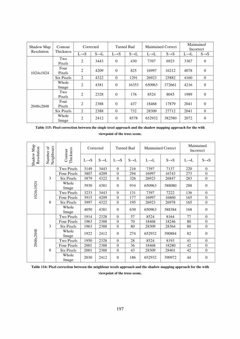
197
Shadow Map
Resolution
Contour
Thickness
Corrected Turned Bad Maintained Correct Maintained
Incorrect
L→S S→L L→S S→L L→L S→S L→L S→S
1024x1024
Two
Pixels 2 3443 0 430 7397 6923 3367 0
Four
Pixels 2 4209 0 825 16997 16212 4078 0
Six Pixels 2 4322 0 1291 26923 25882 4160 0
Whole
Image 2 4381 0 16353 650963 372661 4216 0
2048x2048
Two
Pixels 2 2328 0 176 8524 8045 1989 0
Four
Pixels 2 2388 0 437 18468 17879 2041 0
Six Pixels 2 2388 0 732 28309 27712 2041 0
Whole
Image 2 2412 0 8578 652932 382580 2072 0
Table 115: Pixel correction between the single texel approach and the shadow mapping approach for the with
viewpoint of the trees scene.
Sh
ado
w M
ap
Res
olu
tio
n
Nu
mb
er o
f
Nei
gh
bo
urs
Co
nto
ur
Th
ick
nes
s Corrected Turned Bad Maintained Correct Maintained
Incorrect
L→S S→L L→S S→L L→L S→S L→L S→S
10
24x
102
4 3
Two Pixels 3149 3443 0 216 7397 7137 220 0
Four Pixels 3807 4209 0 294 16997 16743 273 0
Six Pixels 3879 4322 0 326 26923 26847 283 0
Whole
Image 3930 4381 0 934 650963 388080 288 0
8
Two Pixels 3233 3443 0 131 7397 7222 136 0
Four Pixels 3915 4209 0 177 16997 16860 165 0
Six Pixels 3997 4322 0 195 26923 26978 165 0
Whole
Image 4050 4381 0 630 650963 388384 168 0
20
48x
204
8 3
Two Pixels 1914 2328 0 57 8524 8164 77 0
Four Pixels 1963 2388 0 70 18468 18246 80 0
Six Pixels 1963 2388 0 80 28309 28364 80 0
Whole
Image 1922 2412 0 274 652932 390884 82 0
8
Two Pixels 1950 2328 0 28 8524 8193 41 0
Four Pixels 2001 2388 0 36 18468 18280 42 0
Six Pixels 2001 2388 0 43 28309 28401 42 0
Whole
Image 2030 2412 0 186 652932 390972 44 0
Table 116: Pixel correction between the neighbour texels approach and the shadow mapping approach for the with
viewpoint of the trees scene.
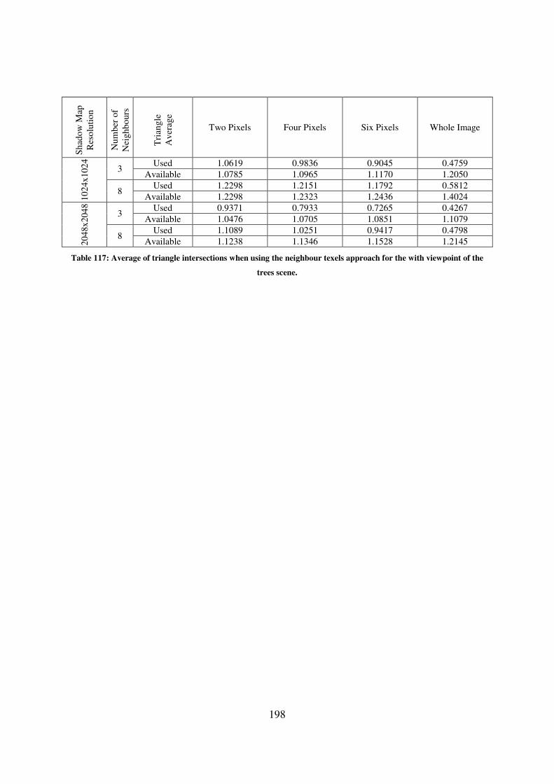
198
Sh
ado
w M
ap
Res
olu
tio
n
Nu
mb
er o
f
Nei
gh
bo
urs
Tri
ang
le
Av
erag
e
Two Pixels Four Pixels Six Pixels Whole Image
10
24x
102
4
3 Used 1.0619 0.9836 0.9045 0.4759
Available 1.0785 1.0965 1.1170 1.2050
8 Used 1.2298 1.2151 1.1792 0.5812
Available 1.2298 1.2323 1.2436 1.4024
20
48x
204
8
3 Used 0.9371 0.7933 0.7265 0.4267
Available 1.0476 1.0705 1.0851 1.1079
8 Used 1.1089 1.0251 0.9417 0.4798
Available 1.1238 1.1346 1.1528 1.2145
Table 117: Average of triangle intersections when using the neighbour texels approach for the with viewpoint of the
trees scene.
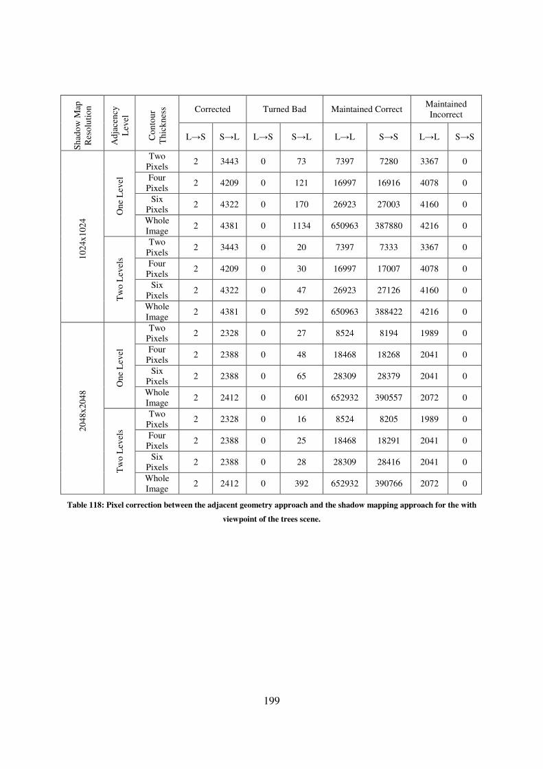
199
Sh
ado
w M
ap
Res
olu
tio
n
Ad
jace
ncy
Lev
el
Co
nto
ur
Th
ick
nes
s Corrected Turned Bad Maintained Correct Maintained
Incorrect
L→S S→L L→S S→L L→L S→S L→L S→S
10
24x
102
4 O
ne
Lev
el
Two
Pixels 2 3443 0 73 7397 7280 3367 0
Four
Pixels 2 4209 0 121 16997 16916 4078 0
Six
Pixels 2 4322 0 170 26923 27003 4160 0
Whole
Image 2 4381 0 1134 650963 387880 4216 0
Tw
o L
evel
s
Two
Pixels 2 3443 0 20 7397 7333 3367 0
Four
Pixels 2 4209 0 30 16997 17007 4078 0
Six
Pixels 2 4322 0 47 26923 27126 4160 0
Whole
Image 2 4381 0 592 650963 388422 4216 0
20
48x
204
8 O
ne
Lev
el
Two
Pixels 2 2328 0 27 8524 8194 1989 0
Four
Pixels 2 2388 0 48 18468 18268 2041 0
Six
Pixels 2 2388 0 65 28309 28379 2041 0
Whole
Image 2 2412 0 601 652932 390557 2072 0
Tw
o L
evel
s
Two
Pixels 2 2328 0 16 8524 8205 1989 0
Four
Pixels 2 2388 0 25 18468 18291 2041 0
Six
Pixels 2 2388 0 28 28309 28416 2041 0
Whole
Image 2 2412 0 392 652932 390766 2072 0
Table 118: Pixel correction between the adjacent geometry approach and the shadow mapping approach for the with
viewpoint of the trees scene.
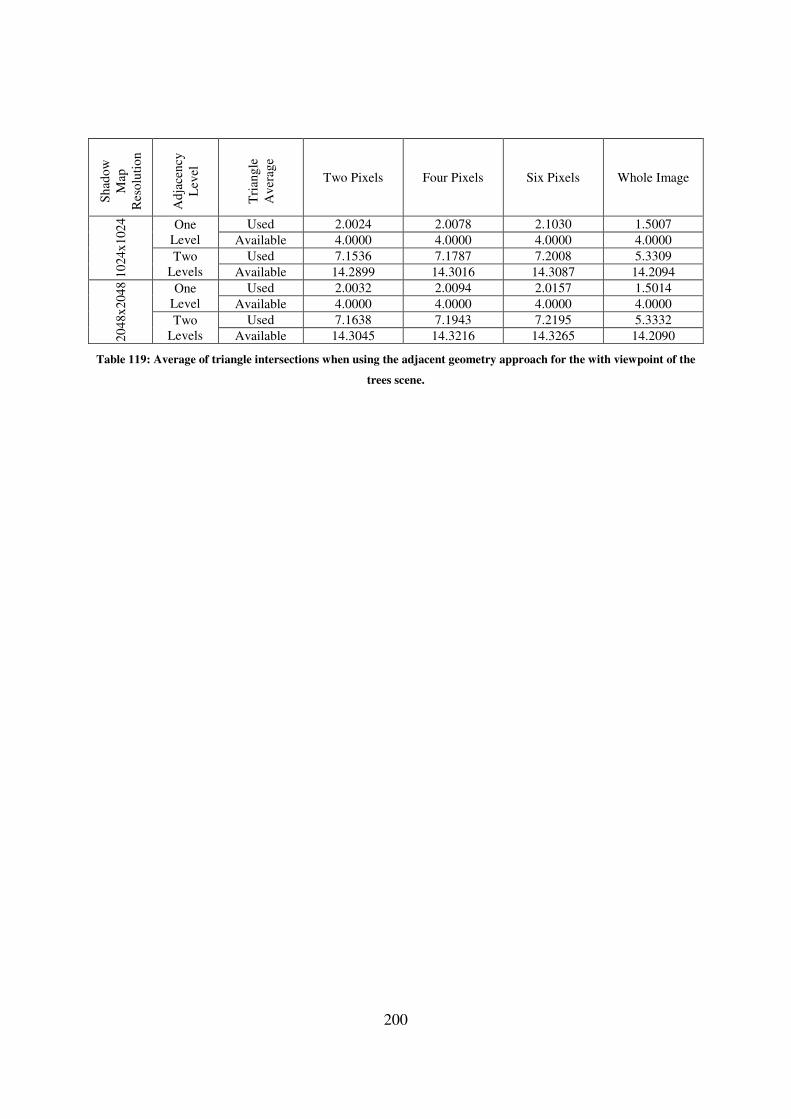
200
Sh
ado
w
Map
Res
olu
tio
n
Ad
jace
ncy
Lev
el
Tri
ang
le
Av
erag
e
Two Pixels Four Pixels Six Pixels Whole Image
10
24x
102
4
One
Level
Used 2.0024 2.0078 2.1030 1.5007
Available 4.0000 4.0000 4.0000 4.0000
Two
Levels
Used 7.1536 7.1787 7.2008 5.3309
Available 14.2899 14.3016 14.3087 14.2094
20
48x
204
8
One
Level
Used 2.0032 2.0094 2.0157 1.5014
Available 4.0000 4.0000 4.0000 4.0000
Two
Levels
Used 7.1638 7.1943 7.2195 5.3332
Available 14.3045 14.3216 14.3265 14.2090
Table 119: Average of triangle intersections when using the adjacent geometry approach for the with viewpoint of the
trees scene.

201
Contour Thickness Two Pixels Four Pixels Six Pixels Whole Image
Lighting L→S S→L L→S S→L L→S S→L L→S S→L
Sh
ado
w M
ap R
eso
luti
on
10
24x
102
4
Corrected by
Both 2 3443 2 4209 2 4322 2 4381
Turned Bad
by Both 0 4 0 4 0 4 0 13
Corrected by
Neighbour
Texels Only
3231 0 3913 0 3995 0 4048 0
Corrected by
Adjacent
Geometry
Only
0 0 0 0 0 0 0 0
Turned Bad
by
Neighbour
Texels Only
0 127 0 173 0 191 0 617
Turned Bad
by Adjacent
Geometry
Only
0 16 0 26 0 43 0 579
20
48x
204
8
Corrected by
Both 2 2328 2 2388 2 2388 2 2412
Turned Bad
by Both 0 3 0 3 0 3 0 3
Corrected by
Neighbour
Texels Only
1948 0 1999 0 1999 0 2028 0
Corrected by
Adjacent
Geometry
Only
0 0 0 0 0 0 0 0
Turned Bad
by
Neighbour
Texels Only
0 25 0 33 0 40 0 183
Turned Bad
by Adjacent
Geometry
Only
0 13 0 22 0 25 0 389
Table 120: Pixel correction by the neighbour texels (9 texels) and the adjacent geometry (2 levels) approaches
separated by lighting change for the with viewpoint of the trees scene.
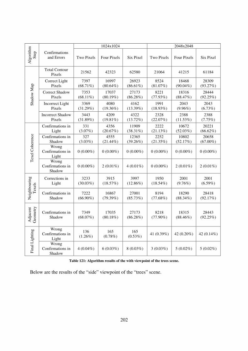
202
Alg
ori
thm
Ste
p
Confirmations
and Errors
1024x1024 2048x2048
Two Pixels Four Pixels Six Pixel Two Pixels Four Pixels Six Pixel
Sh
ado
w M
ap
Total Contour
Pixels 21562 42323 62580 21064 41215 61184
Correct Light
Pixels
7397
(68.71%)
16997
(80.64%)
26923
(86.61%)
8524
(81.07%)
18468
(90.04%)
28309
(93.27%)
Correct Shadow
Pixels
7353
(68.11%)
17037
(80.19%)
27173
(86.28%)
8221
(77.93%)
18316
(88.47%)
28444
(92.25%)
Incorrect Light
Pixels
3369
(31.29%)
4080
(19.36%)
4162
(13.39%)
1991
(18.93%)
2043
(9.96%)
2043
(6.73%)
Incorrect Shadow
Pixels
3443
(31.89%)
4209
(19.81%)
4322
(13.72%)
2328
(22.07%)
2388
(11.53%)
2388
(7.75%)
Tex
el C
oh
eren
ce
Confirmations in
Light
331
(3.07%)
4356
(20.67%)
11909
(38.31%)
2222
(21.13%)
10672
(52.03%)
20221
(66.62%)
Confirmations in
Shadow
327
(3.03%)
4555
(21.44%)
12365
(39.26%)
2252
(21.35%)
10802
(52.17%)
20658
(67.00%)
Wrong
Confirmations in
Light
0 (0.00%) 0 (0.00%) 0 (0.00%) 0 (0.00%) 0 (0.00%) 0 (0.00%)
Wrong
Confirmations in
Shadow
0 (0.00%) 2 (0.01%) 4 (0.01%) 0 (0.00%) 2 (0.01%) 2 (0.01%)
Nei
gh
bo
uri
ng
Tex
els
Corrections in
Light
3233
(30.03%)
3915
(18.57%)
3997
(12.86%)
1950
(18.54%)
2001
(9.76%)
2001
(6.59%)
Confirmations in
Shadow
7222
(66.90%)
16867
(79.39%)
27001
(85.73%)
8194
(77.68%)
18290
(88.34%)
28418
(92.17%)
Ad
jace
nt
Geo
met
ry
Confirmations in
Shadow
7349
(68.07%)
17035
(80.18%)
27173
(86.28%)
8218
(77.90%)
18315
(88.46%)
28443
(92.25%)
Fin
al L
igh
tin
g Wrong
Confirmations in
Light
136
(1.26%)
165
(0.78%)
165
(0.53%) 41 (0.39%) 42 (0.20%) 42 (0.14%)
Wrong
Confirmations in
Shadow
4 (0.04%) 6 (0.03%) 8 (0.03%) 3 (0.03%) 5 (0.02%) 5 (0.02%)
Table 121: Algorithm results of the with viewpoint of the trees scene.
Below are the results of the “side” viewpoint of the “trees” scene.
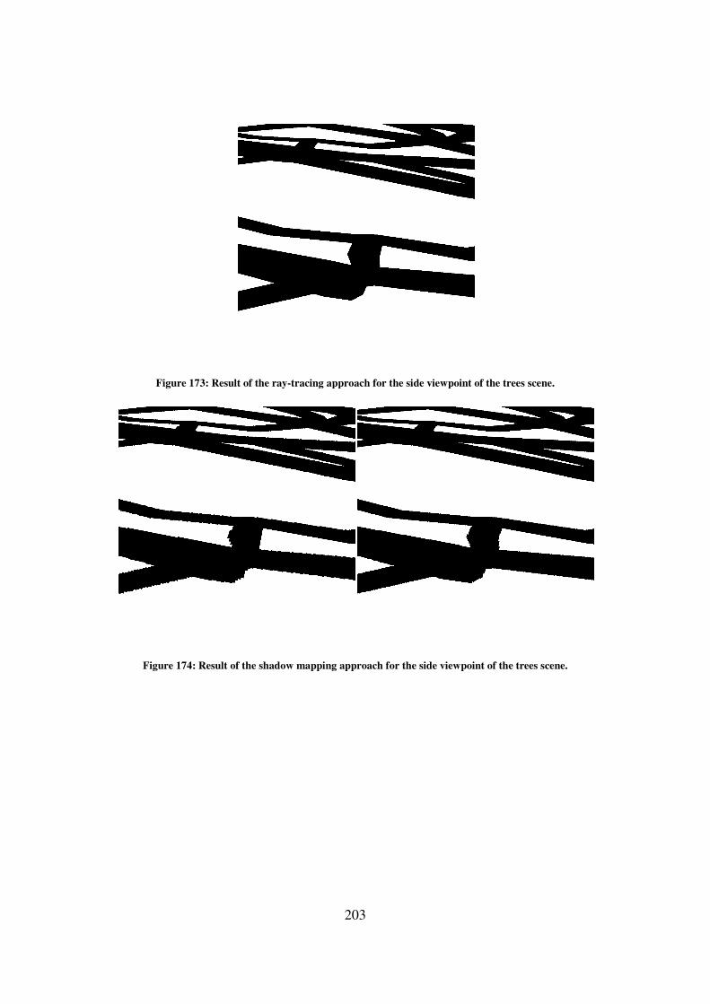
Figure 173: Result of the ray
Figure 174: Result of the shadow mapping approach for the
203
: Result of the ray-tracing approach for the side viewpoint of the trees scene.
: Result of the shadow mapping approach for the side viewpoint of the
tracing approach for the side viewpoint of the trees scene.
viewpoint of the trees scene.
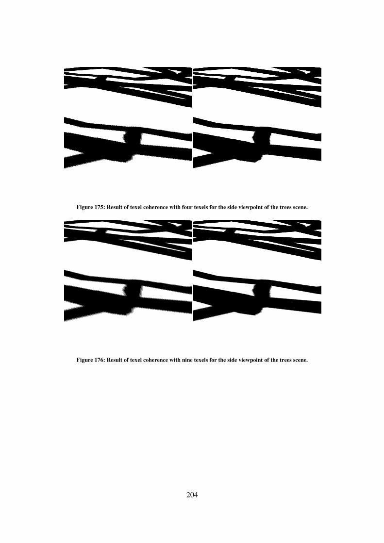
Figure 175: Result of texel coherence with four texels for
Figure 176: Result of texel coherence with nine texels for
204
: Result of texel coherence with four texels for the side viewpoint of the trees scene
: Result of texel coherence with nine texels for the side viewpoint of the trees scene
the side viewpoint of the trees scene.
wpoint of the trees scene.
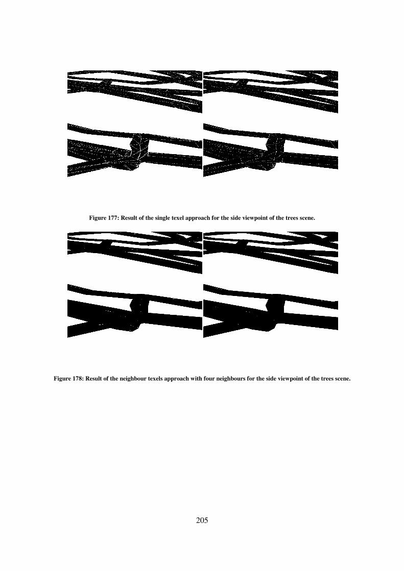
205
Figure 177: Result of the single texel approach for the side viewpoint of the trees scene.
Figure 178: Result of the neighbour texels approach with four neighbours for the side viewpoint of the trees scene.
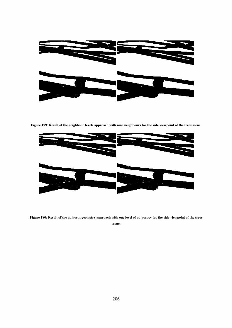
206
Figure 179: Result of the neighbour texels approach with nine neighbours for the side viewpoint of the trees scene.
Figure 180: Result of the adjacent geometry approach with one level of adjacency for the side viewpoint of the trees
scene.
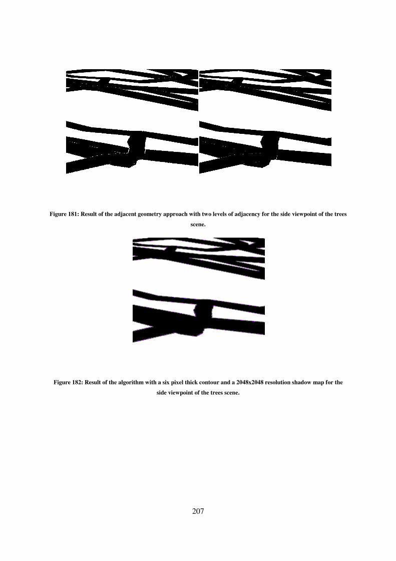
Figure 181: Result of the adjacent geometry
Figure 182: Result of the algorithm with a six pixel thick contour and a 2048x2048 resolution shadow map for the
207
adjacent geometry approach with two levels of adjacency for the side viewpoint of the trees
scene.
: Result of the algorithm with a six pixel thick contour and a 2048x2048 resolution shadow map for the
side viewpoint of the trees scene.
the side viewpoint of the trees
: Result of the algorithm with a six pixel thick contour and a 2048x2048 resolution shadow map for the

208
Figure 183: Corrected/confirmed/hinted contour pixels by each method for the side viewpoint of the trees scene using
a 1024x1024 (top) and a 2048x2048 (bottom) resolution shadow map.
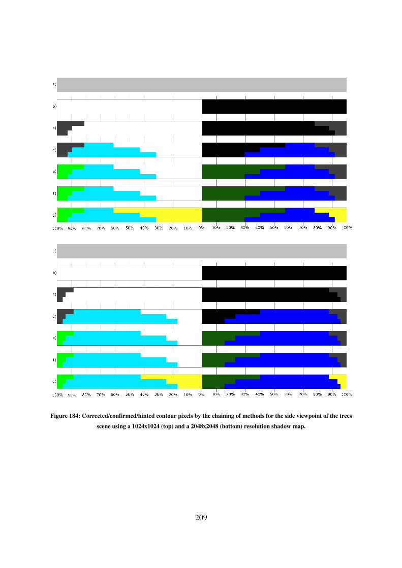
209
Figure 184: Corrected/confirmed/hinted contour pixels by the chaining of methods for the side viewpoint of the trees
scene using a 1024x1024 (top) and a 2048x2048 (bottom) resolution shadow map.

210
Shadow Map
Resolution Approach
Contour Thickness
Two Pixels Four Pixels Six Pixels Whole Image
1024x1024
Pixels in
Contour 27414 54182 80266 1048576
Shadow Map 5602 (20.43%) 6161 (11.37%) 6254 (7.79%) 6349 (0.61%)
Single Texel 3021 (11.02%) 3831 (7.07%) 4594 (5.72%) 20004 (1.91%)
Neighbour
Texels (4
Neighbours)
215 (0.78%) 257 (0.47%) 306 (0.38%) 984 (0.09%)
Neighbour
Texels (9
Neighbours)
90 (0.33%) 101 (0.19%) 121 (0.15%) 503 (0.05%)
Adjacent
Geometry (One
Level)
2640 (9.63%) 2928 (5.40%) 3027 (3.77%) 4635 (0.44%)
Adjacent
Geometry
(Two Level)
2601 (9.49%) 2852 (5.26%) 2906 (3.62%) 4127 (0.39%)
2048x2048
Pixels in
Contour 27267 53603 79206 1048576
Shadow Map 3198 (11.73%) 3256 (6.07%) 3257 (4.11%) 3283 (0.31%)
Single Texel 1788 (6.56%) 2135 (3.98%) 2460 (3.11%) 10338 (0.99%)
Neighbour
Texels (4
Neighbours)
60 (0.22%) 70 (0.13%) 87 (0.11%) 264 (0.03%)
Neighbour
Texels (9
Neighbours)
25 (0.09%) 26 (0.05%) 36 (0.05%) 153 (0.01%)
Adjacent
Geometry (One
Level)
1553 (5.70%) 1601 (2.99%) 1628 (2.06%) 2292 (0.22%)
Adjacent
Geometry
(Two Level)
1545 (5.67%) 1581 (2.95%) 1589 (2.01%) 2114 (0.20%)
Table 122: Difference between the approaches that use ray-tracing and the actual ray-tracer for the side viewpoint of
the trees scene.
Shadow Map Resolution Contour Thickness
Two Pixels Four Pixels Six Pixels
1024x1024 5602 of 6349 (88.23%) 6161 of 6349 (97.04%) 6254 of 6349 (98.50%)
2048x2048 3198 of 3283 (97.41%) 3256 of 3283 (99.18%) 3257 of 3283 (99.21%)
Table 123: Wrongly defined pixels in the shadow mapping result which are inside the contour in the side viewpoint of
the trees scene.

211
Shadow Map Resolution Contour Thickness Pixel Shading
Light Shadow
1024x1024
Two Pixels 2579 of 13645 3023 of 13769
Four Pixels 2811 of 26799 3350 of 27383
Six Pixels 2843 of 39347 3411 of 40919
Whole Image 2884 of 675205 3465 of 373371
2048x2048
Two Pixels 1528 of 13557 1670 of 13710
Four Pixels 1552 of 26440 1704 of 27163
Six Pixels 1552 of 38742 1705 of 40464
Whole Image 1564 of 675631 1719 of 372945
Table 124: Pixels that the shadow map defines wrongly in the side viewpoint of the trees scene, separated in pixels
defined in light and in shadow, compared to the total amount of pixels lighted in the same way.
Shadow
Map
Resolution
Contour
Thickness
Texel Coherence
Light Shadow
Confirmed Incorrectly
Confirmed Undecided Confirmed
Incorrectly
Confirmed Undecided
1024x1024
Two Pixels 2722
(19.95%) 0 (0.00%)
10923
(80.05%)
2813
(20.43%) 0 (0.00%)
10956
(79.57%)
Four Pixels 12457
(46.48%) 0 (0.00%)
14342
(53.52%)
12960
(47.33%) 0 (0.00%)
14423
(52.67%)
Six Pixels 24007
(61.01%) 0 (0.00%)
15340
(38.99%)
25434
(62.16%) 1 (0.00%)
15485
(37.84%)
Whole
Image
659046
(97.61%) 0 (0.00%)
16159
(2.39%)
357046
(95.63%) 11 (0.00%)
16325
(4.37%)
2048x2048
Two Pixels 6288
(46.38%) 0 (0.00%)
7269
(53.62%)
6514
(47.51%) 0 (0.00%)
7196
(52.49%)
Four Pixels 18358
(69.43%) 0 (0.00%)
8082
(30.57%)
19155
(70.52%) 0 (0.00%)
8008
(29.48%)
Six Pixels 30604
(78.99%) 0 (0.00%)
8138
(21.01%)
32399
(80.07%) 0 (0.00%)
8065
(19.93%)
Whole
Image
667411
(98.78%) 0 (0.00%)
8220
(1.22%)
364797
(97.82%) 0 (0.00%)
8148
(2.18%)
Table 125: Pixel confirmation when using texel coherence with four texels for the side viewpoint of the trees scene.
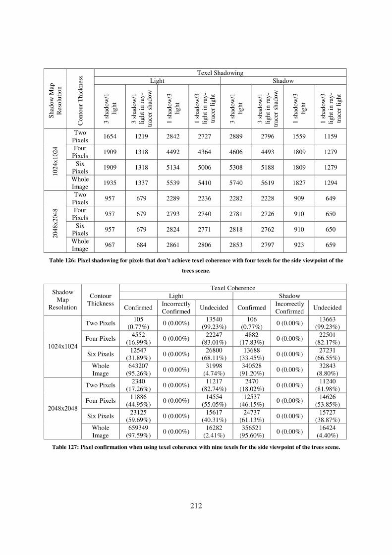
212
Sh
ado
w M
ap
Res
olu
tio
n
Co
nto
ur
Th
ick
nes
s Texel Shadowing
Light Shadow
3 s
had
ow
/1
lig
ht
3 s
had
ow
/1
lig
ht
in r
ay-
trac
er s
had
ow
1 s
had
ow
/3
lig
ht
1 s
had
ow
/3
lig
ht
in r
ay-
trac
er l
igh
t
3 s
had
ow
/1
lig
ht
3 s
had
ow
/1
lig
ht
in r
ay-
trac
er s
had
ow
1 s
had
ow
/3
lig
ht
1 s
had
ow
/3
lig
ht
in r
ay-
trac
er l
igh
t
10
24x
102
4
Two
Pixels 1654 1219 2842 2727 2889 2796 1559 1159
Four
Pixels 1909 1318 4492 4364 4606 4493 1809 1279
Six
Pixels 1909 1318 5134 5006 5308 5188 1809 1279
Whole
Image 1935 1337 5539 5410 5740 5619 1827 1294
20
48x
204
8
Two
Pixels 957 679 2289 2236 2282 2228 909 649
Four
Pixels 957 679 2793 2740 2781 2726 910 650
Six
Pixels 957 679 2824 2771 2818 2762 910 650
Whole
Image 967 684 2861 2806 2853 2797 923 659
Table 126: Pixel shadowing for pixels that don’t achieve texel coherence with four texels for the side viewpoint of the
trees scene.
Shadow
Map
Resolution
Contour
Thickness
Texel Coherence
Light Shadow
Confirmed Incorrectly
Confirmed Undecided Confirmed
Incorrectly
Confirmed Undecided
1024x1024
Two Pixels 105
(0.77%) 0 (0.00%)
13540
(99.23%)
106
(0.77%) 0 (0.00%)
13663
(99.23%)
Four Pixels 4552
(16.99%) 0 (0.00%)
22247
(83.01%)
4882
(17.83%) 0 (0.00%)
22501
(82.17%)
Six Pixels 12547
(31.89%) 0 (0.00%)
26800
(68.11%)
13688
(33.45%) 0 (0.00%)
27231
(66.55%)
Whole
Image
643207
(95.26%) 0 (0.00%)
31998
(4.74%)
340528
(91.20%) 0 (0.00%)
32843
(8.80%)
2048x2048
Two Pixels 2340
(17.26%) 0 (0.00%)
11217
(82.74%)
2470
(18.02%) 0 (0.00%)
11240
(81.98%)
Four Pixels 11886
(44.95%) 0 (0.00%)
14554
(55.05%)
12537
(46.15%) 0 (0.00%)
14626
(53.85%)
Six Pixels 23125
(59.69%) 0 (0.00%)
15617
(40.31%)
24737
(61.13%) 0 (0.00%)
15727
(38.87%)
Whole
Image
659349
(97.59%) 0 (0.00%)
16282
(2.41%)
356521
(95.60%) 0 (0.00%)
16424
(4.40%)
Table 127: Pixel confirmation when using texel coherence with nine texels for the side viewpoint of the trees scene.
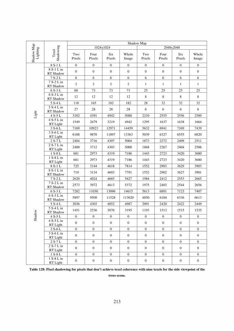
213
Sh
ado
w M
ap
Lig
hti
ng
Tex
el
Sh
ado
win
g Shadow Map
1024x1024 2048x2048
Two
Pixels
Four
Pixels
Six
Pixels
Whole
Image
Two
Pixels
Four
Pixels
Six
Pixels
Whole
Image
Lig
ht
8 S-1 L 0 0 0 0 0 0 0 0
8 S-1 L in
RT Shadow 0 0 0 0 0 0 0 0
7 S-2 L 6 6 6 6 6 6 6 6
7 S-2 L in
RT Shadow 2 2 2 2 1 1 1 1
6 S-3 L 60 73 73 73 25 25 25 25
6 S-3 L in
RT Shadow 12 12 12 12 8 8 8 8
5 S-4 L 118 165 182 182 28 32 32 32
5 S-4 L in
RT Shadow 27 28 28 28 6 6 6 6
4 S-5 L 3102 4391 4942 5088 2210 2555 2556 2589
4 S-5 L in
RT Light 1549 2679 3219 4942 1295 1637 1638 1664
3 S-6 L 7169 10923 12971 14459 5632 6941 7169 7439
3 S-6 L in
RT Light 6188 9870 11897 13363 5039 6327 6555 6820
2 S-7 L 2404 3716 4307 5004 1873 2272 2409 2511
2 S-7 L in
RT Light 2400 3712 4303 5000 1868 2267 2404 2506
1 S-8 L 681 2973 4319 7186 1443 2723 3420 3680
1 S-8 L in
RT Light 681 2973 4319 7186 1443 2723 3420 3680
Sh
ado
w
8 S-1 L 725 3144 4618 7814 1552 2903 3629 3903
8 S-1 L in
RT Shadow 719 3134 4603 7791 1552 2902 3627 3901
7 S-2 L 2620 4024 4665 5427 1984 2412 2553 2665
7 S-2 L in
RT Shadow 2573 3972 4613 5372 1975 2403 2544 2656
6 S-3 L 7282 11030 13096 14615 5613 6891 7123 7407
6 S-3 L in
RT Shadow 5897 9509 11528 113020 4850 6104 6336 6613
5 S-4 L 3036 4303 4852 4987 2091 2420 2422 2449
5 S-4 L in
RT Shadow 1451 2536 3076 3195 1193 1513 1515 1535
4 S-5 L 0 0 0 0 0 0 0 0
4 S-5 L in
RT Light 0 0 0 0 0 0 0 0
3 S-6 L 0 0 0 0 0 0 0 0
3 S-6 L in
RT Light 0 0 0 0 0 0 0 0
2 S-7 L 0 0 0 0 0 0 0 0
2 S-7 L in
RT Light 0 0 0 0 0 0 0 0
1 S-8 L 0 0 0 0 0 0 0 0
1 S-8 L in
RT Light 0 0 0 0 0 0 0 0
Table 128: Pixel shadowing for pixels that don’t achieve texel coherence with nine texels for the side viewpoint of the
trees scene.

214
Shadow Map
Resolution
Contour
Thickness
Corrected Turned Bad Maintained Correct Maintained
Incorrect
L→S S→L L→S S→L L→L S→S L→L S→S
1024x1024
Two Pixels 0 3023 0 442 11066 10304 2579 0
Four Pixels 0 3350 0 1020 23988 23013 2811 0
Six Pixels 0 3411 0 1751 36504 35757 2843 0
Whole Image 0 3465 0 17120 672321 352786 2884 0
2048x2048
Two Pixels 1 1670 0 261 12029 11779 1527 0
Four Pixels 1 1704 0 584 24888 24875 1551 0
Six Pixels 1 1705 0 909 37190 37850 1551 0
Whole Image 1 1719 0 8775 674067 362451 1563 0
Table 129: Pixel correction between the single texel approach and the shadow mapping approach for the side
viewpoint of the trees scene.
Shadow Map
Resolution
Contour
Thickness
Corrected Turned Bad Maintained Correct Maintained
Incorrect
L→S S→L L→S S→L L→L S→S L→L S→S
1024x1024
Two Pixels 2463 3023 0 99 11066 10647 116 0
Four Pixels 2690 3350 0 136 23988 23897 121 0
Six Pixels 2722 3411 0 185 36504 37323 121 0
Whole Image 2763 3465 0 863 672321 369043 121 0
2048x2048
Two Pixels 1496 1670 0 28 12029 12012 32 0
Four Pixels 1520 1704 0 38 24888 25421 32 0
Six Pixels 1520 1705 0 55 37190 38704 32 0
Whole Image 1532 1719 0 232 674067 370994 32 0
Table 130: Pixel correction between the neighbour texels approach using four neighbours and the shadow mapping
approach for the side viewpoint of the trees scene.
Shadow Map
Resolution
Contour
Thickness
Corrected Turned Bad Maintained Correct Maintained
Incorrect
L→S S→L L→S S→L L→L S→S L→L S→S
1024x1024
Two Pixels 2523 3023 0 34 11066 10712 56 0
Four Pixels 2753 3350 0 43 23988 23990 58 0
Six Pixels 2785 3411 0 63 36504 37445 58 0
Whole Image 2826 3465 0 445 672321 369461 58 0
2048x2048
Two Pixels 1512 1670 0 9 12029 12031 16 0
Four Pixels 1536 1704 0 10 24888 25449 16 0
Six Pixels 1536 1705 0 20 37190 38739 16 0
Whole Image 1548 1719 0 137 674067 371089 16 0
Table 131: Pixel correction between the neighbour texels approach using nine neighbours and the shadow mapping
approach for the side viewpoint of the trees scene.
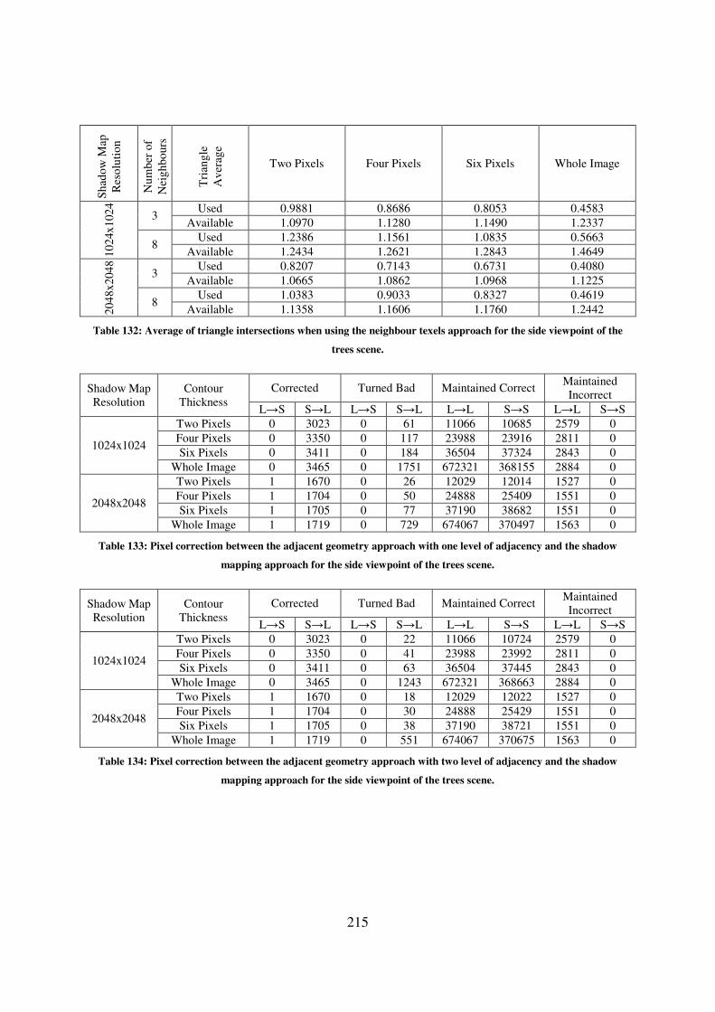
215
Sh
ado
w M
ap
Res
olu
tio
n
Nu
mb
er o
f
Nei
gh
bo
urs
Tri
ang
le
Av
erag
e
Two Pixels Four Pixels Six Pixels Whole Image
10
24x
102
4
3 Used 0.9881 0.8686 0.8053 0.4583
Available 1.0970 1.1280 1.1490 1.2337
8 Used 1.2386 1.1561 1.0835 0.5663
Available 1.2434 1.2621 1.2843 1.4649
20
48x
204
8
3 Used 0.8207 0.7143 0.6731 0.4080
Available 1.0665 1.0862 1.0968 1.1225
8 Used 1.0383 0.9033 0.8327 0.4619
Available 1.1358 1.1606 1.1760 1.2442
Table 132: Average of triangle intersections when using the neighbour texels approach for the side viewpoint of the
trees scene.
Shadow Map
Resolution
Contour
Thickness
Corrected Turned Bad Maintained Correct Maintained
Incorrect
L→S S→L L→S S→L L→L S→S L→L S→S
1024x1024
Two Pixels 0 3023 0 61 11066 10685 2579 0
Four Pixels 0 3350 0 117 23988 23916 2811 0
Six Pixels 0 3411 0 184 36504 37324 2843 0
Whole Image 0 3465 0 1751 672321 368155 2884 0
2048x2048
Two Pixels 1 1670 0 26 12029 12014 1527 0
Four Pixels 1 1704 0 50 24888 25409 1551 0
Six Pixels 1 1705 0 77 37190 38682 1551 0
Whole Image 1 1719 0 729 674067 370497 1563 0
Table 133: Pixel correction between the adjacent geometry approach with one level of adjacency and the shadow
mapping approach for the side viewpoint of the trees scene.
Shadow Map
Resolution
Contour
Thickness
Corrected Turned Bad Maintained Correct Maintained
Incorrect
L→S S→L L→S S→L L→L S→S L→L S→S
1024x1024
Two Pixels 0 3023 0 22 11066 10724 2579 0
Four Pixels 0 3350 0 41 23988 23992 2811 0
Six Pixels 0 3411 0 63 36504 37445 2843 0
Whole Image 0 3465 0 1243 672321 368663 2884 0
2048x2048
Two Pixels 1 1670 0 18 12029 12022 1527 0
Four Pixels 1 1704 0 30 24888 25429 1551 0
Six Pixels 1 1705 0 38 37190 38721 1551 0
Whole Image 1 1719 0 551 674067 370675 1563 0
Table 134: Pixel correction between the adjacent geometry approach with two level of adjacency and the shadow
mapping approach for the side viewpoint of the trees scene.
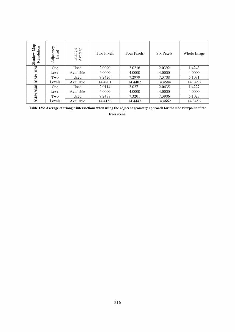
216
Sh
ado
w M
ap
Res
olu
tio
n
Ad
jace
ncy
Lev
el
Tri
ang
le
Av
erag
e
Two Pixels Four Pixels Six Pixels Whole Image
10
24x
102
4
One
Level
Used 2.0090 2.0216 2.0392 1.4243
Available 4.0000 4.0000 4.0000 4.0000
Two
Levels
Used 7.2426 7.2979 7.3708 5.1081
Available 14.4201 14.4402 14.4584 14.3456
20
48x
204
8
One
Level
Used 2.0114 2.0271 2.0435 1.4227
Available 4.0000 4.0000 4.0000 4.0000
Two
Levels
Used 7.2488 7.3201 7.3906 5.1023
Available 14.4156 14.4447 14.4662 14.3456
Table 135: Average of triangle intersections when using the adjacent geometry approach for the side viewpoint of the
trees scene.

217
Contour Thickness Two Pixels Four Pixels Six Pixels Whole Image
Lighting L→S S→L L→S S→L L→S S→L L→S S→L
Sh
ado
w M
ap R
eso
luti
on
10
24x
102
4
Corrected by
Both 0 3023 0 3350 0 3411 0 3465
Turned Bad
by Both 0 5 0 5 0 5 0 14
Corrected by
Neighbour
Texels Only
2523 0 2753 0 2785 0 2826 0
Corrected by
Adjacent
Geometry
Only
0 0 0 0 0 0 0 0
Turned Bad
by
Neighbour
Texels Only
0 29 0 38 0 58 0 431
Turned Bad
by Adjacent
Geometry
Only
0 17 0 36 0 58 0 1229
20
48x
204
8
Corrected by
Both 1 1670 1 1704 1 1705 1 1719
Turned Bad
by Both 0 1 0 1 0 1 0 9
Corrected by
Neighbour
Texels Only
1511 0 1535 0 1535 0 1547 0
Corrected by
Adjacent
Geometry
Only
0 0 0 0 0 0 0 0
Turned Bad
by
Neighbour
Texels Only
0 8 0 9 0 19 0 128
Turned Bad
by Adjacent
Geometry
Only
0 17 0 29 0 37 0 542
Table 136: Pixel correction by the neighbour texels (9 texels) and the adjacent geometry (2 levels) approaches
separated by lighting change for the side viewpoint of the trees scene.

218
Alg
ori
thm
Ste
p
Confirmations
and Errors
1024x1024 2048x2048
Two Pixels Four Pixels Six Pixel Two Pixels Four Pixels Six Pixel
Sh
ado
w M
ap
Total Contour
Pixels 27414 54182 80266 27267 53603 79206
Correct Light
Pixels
11066
(81.10%)
23988
(89.51%)
36504
(92.77%)
12029
(88.73%)
24888
(94.13%)
37190
(95.99%)
Correct Shadow
Pixels
10746
(78.04%)
24033
(87.77%)
37508
(91.66%)
12040
(87.82%)
25459
(93.73%)
38759
(95.79%)
Incorrect Light
Pixels
2579
(18.90%)
2811
(10.49%)
2843
(7.23%)
1528
(11.27%)
1552
(5.87%)
1552
(4.01%)
Incorrect Shadow
Pixels
3023
(21.96%)
3350
(12.23%)
3411
(8.34%)
1670
(12.18%)
1704
(6.27%)
1705
(4.21%)
Tex
el C
oh
eren
ce
Confirmations in
Light
2722
(19.95%)
12457
(46.48%)
24007
(61.01%)
6288
(46.38%)
18358
(69.43%)
30604
(78.99%)
Confirmations in
Shadow
2813
(20.43%)
12960
(47.33%)
25434
(62.16%)
6514
(47.51%)
19155
(70.52%)
32399
(80.07%)
Wrong
Confirmations in
Light
0 (0.00%) 0 (0.00%) 0 (0.00%) 0 (0.00%) 0 (0.00%) 0 (0.00%)
Wrong
Confirmations in
Shadow
0 (0.00%) 0 (0.00%) 1 (0.00%) 0 (0.00%) 0 (0.00%) 0 (0.00%)
Nei
gh
bo
uri
ng
Tex
els
Corrections in
Light
2523
(18.49%)
2753
(10.27%)
2785
(7.08%)
1512
(11.15%)
1536
(5.81%)
1536
(3.96%)
Confirmations in
Shadow
10714
(77.81%)
23994
(87.62%)
37468
(91.57%)
12032
(87.76%)
25450
(93.69%)
38750
(95.76%)
Ad
jace
nt
Geo
met
ry
Confirmations in
Shadow
10741
(78.01%)
24028
(87.75%)
37504
(91.65%)
12039
(87.81%)
25458
(93.72%)
38758
(95.78%)
Fin
al L
igh
tin
g Wrong
Confirmations in
Light
56 (0.41%) 58 (0.22%) 58 (0.15%) 16 (0.12%) 16 (0.06%) 16 (0.04%)
Wrong
Confirmations in
Shadow
5 (0.04%) 5 (0.02%) 6 (0.01%) 1 (0.01%) 1 (0.00%) 1 (0.00%)
Table 137: Algorithm results of the side viewpoint of the trees scene.
Following below are the results for the “against” viewpoint of the “trees” scene.
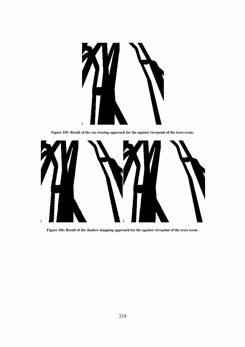
Figure 185: Result of the ray
Figure 186: Result of the shadow mapping approach for the
219
: Result of the ray-tracing approach for the against viewpoint of the trees scene.
: Result of the shadow mapping approach for the against viewpoint of the
tracing approach for the against viewpoint of the trees scene.
of the trees scene.
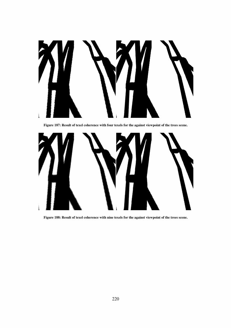
Figure 187: Result of texel coherence with four texels for
Figure 188: Result of texel coherence with nine texels for
220
: Result of texel coherence with four texels for the against viewpoint of the trees scene
: Result of texel coherence with nine texels for the against viewpoint of the trees scene
the against viewpoint of the trees scene.
viewpoint of the trees scene.
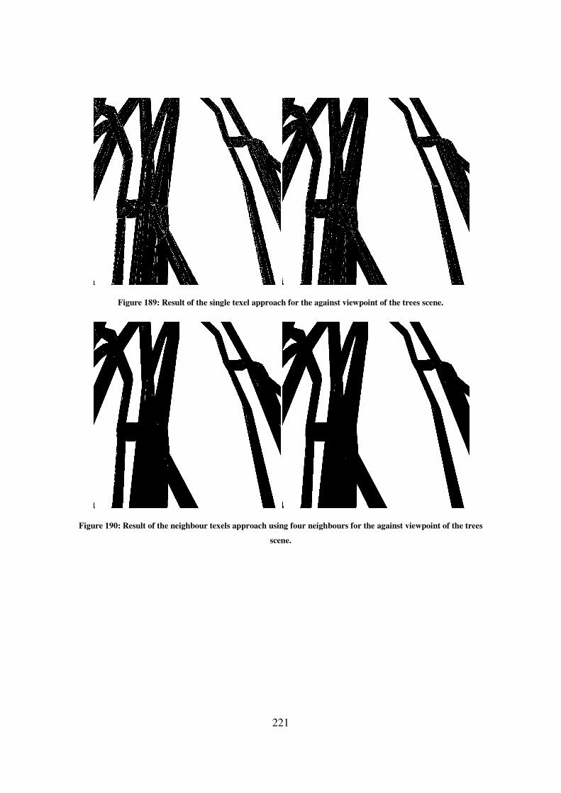
221
Figure 189: Result of the single texel approach for the against viewpoint of the trees scene.
Figure 190: Result of the neighbour texels approach using four neighbours for the against viewpoint of the trees
scene.
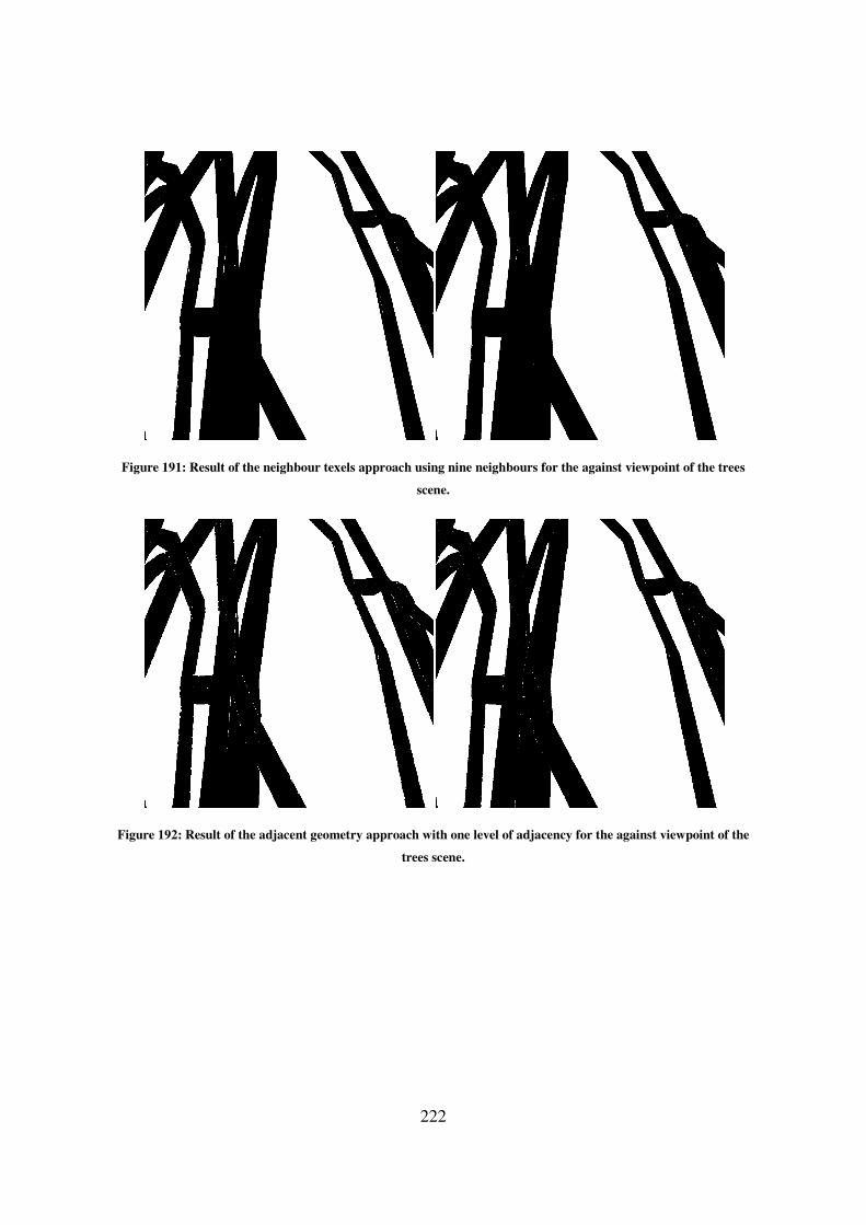
222
Figure 191: Result of the neighbour texels approach using nine neighbours for the against viewpoint of the trees
scene.
Figure 192: Result of the adjacent geometry approach with one level of adjacency for the against viewpoint of the
trees scene.
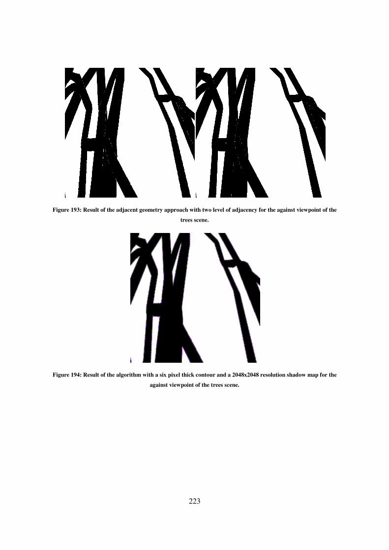
Figure 193: Result of the adjacent geometry
Figure 194: Result of the algorithm with a six pixel thick contour and a 2048x2048 resolution shadow map for the
223
adjacent geometry approach with two level of adjacency for the against viewpoint of the
trees scene.
: Result of the algorithm with a six pixel thick contour and a 2048x2048 resolution shadow map for the
against viewpoint of the trees scene.
the against viewpoint of the
: Result of the algorithm with a six pixel thick contour and a 2048x2048 resolution shadow map for the
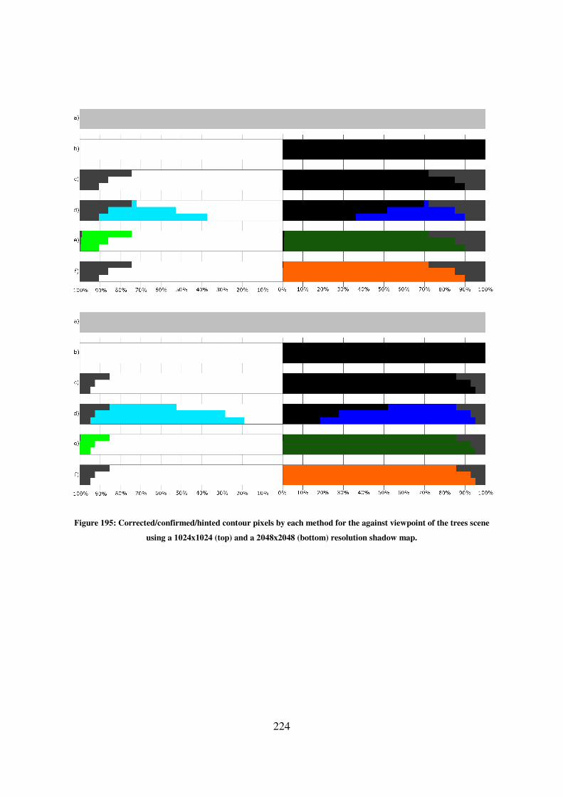
224
Figure 195: Corrected/confirmed/hinted contour pixels by each method for the against viewpoint of the trees scene
using a 1024x1024 (top) and a 2048x2048 (bottom) resolution shadow map.
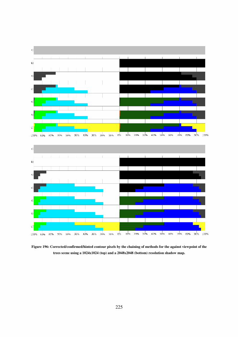
225
Figure 196: Corrected/confirmed/hinted contour pixels by the chaining of methods for the against viewpoint of the
trees scene using a 1024x1024 (top) and a 2048x2048 (bottom) resolution shadow map.
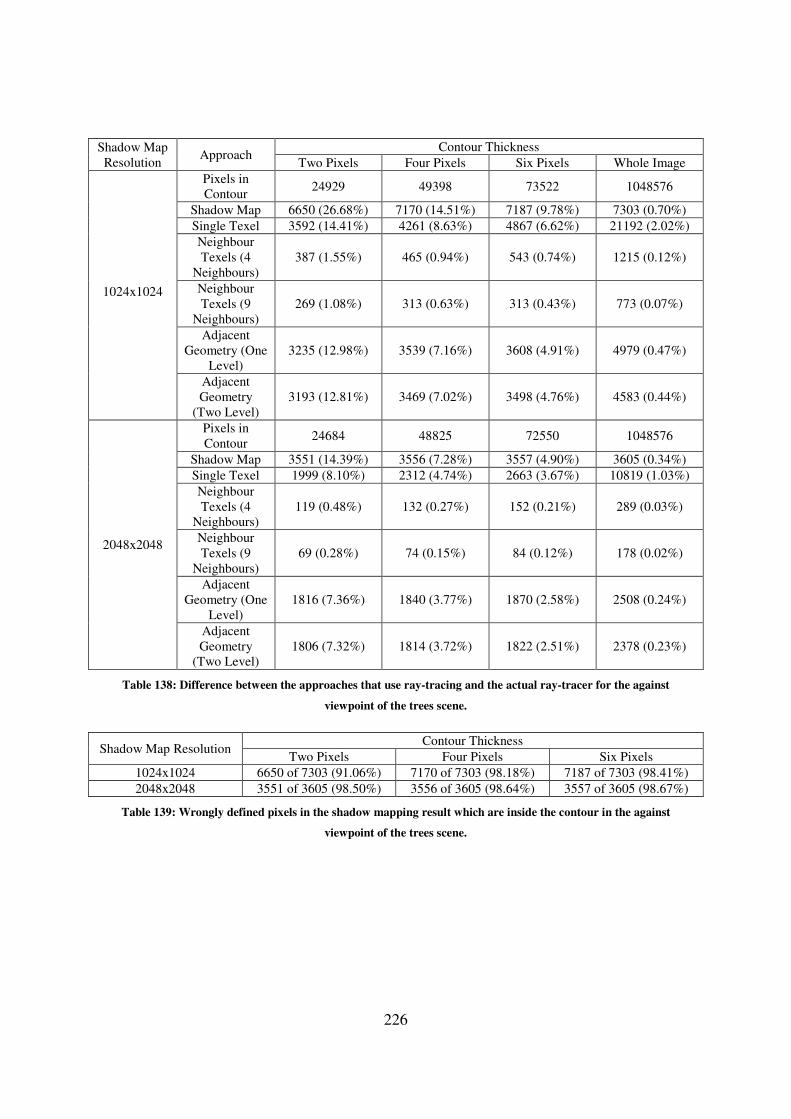
226
Shadow Map
Resolution Approach
Contour Thickness
Two Pixels Four Pixels Six Pixels Whole Image
1024x1024
Pixels in
Contour 24929 49398 73522 1048576
Shadow Map 6650 (26.68%) 7170 (14.51%) 7187 (9.78%) 7303 (0.70%)
Single Texel 3592 (14.41%) 4261 (8.63%) 4867 (6.62%) 21192 (2.02%)
Neighbour
Texels (4
Neighbours)
387 (1.55%) 465 (0.94%) 543 (0.74%) 1215 (0.12%)
Neighbour
Texels (9
Neighbours)
269 (1.08%) 313 (0.63%) 313 (0.43%) 773 (0.07%)
Adjacent
Geometry (One
Level)
3235 (12.98%) 3539 (7.16%) 3608 (4.91%) 4979 (0.47%)
Adjacent
Geometry
(Two Level)
3193 (12.81%) 3469 (7.02%) 3498 (4.76%) 4583 (0.44%)
2048x2048
Pixels in
Contour 24684 48825 72550 1048576
Shadow Map 3551 (14.39%) 3556 (7.28%) 3557 (4.90%) 3605 (0.34%)
Single Texel 1999 (8.10%) 2312 (4.74%) 2663 (3.67%) 10819 (1.03%)
Neighbour
Texels (4
Neighbours)
119 (0.48%) 132 (0.27%) 152 (0.21%) 289 (0.03%)
Neighbour
Texels (9
Neighbours)
69 (0.28%) 74 (0.15%) 84 (0.12%) 178 (0.02%)
Adjacent
Geometry (One
Level)
1816 (7.36%) 1840 (3.77%) 1870 (2.58%) 2508 (0.24%)
Adjacent
Geometry
(Two Level)
1806 (7.32%) 1814 (3.72%) 1822 (2.51%) 2378 (0.23%)
Table 138: Difference between the approaches that use ray-tracing and the actual ray-tracer for the against
viewpoint of the trees scene.
Shadow Map Resolution Contour Thickness
Two Pixels Four Pixels Six Pixels
1024x1024 6650 of 7303 (91.06%) 7170 of 7303 (98.18%) 7187 of 7303 (98.41%)
2048x2048 3551 of 3605 (98.50%) 3556 of 3605 (98.64%) 3557 of 3605 (98.67%)
Table 139: Wrongly defined pixels in the shadow mapping result which are inside the contour in the against
viewpoint of the trees scene.

227
Shadow Map Resolution Contour Thickness Pixel Shading
Light Shadow
1024x1024
Two Pixels 3162 of 12442 3488 of 12487
Four Pixels 3423 of 24570 3747 of 24828
Six Pixels 3430 of 36416 3757 of 37106
Whole Image 3491 of 626198 3812 of 422378
2048x2048
Two Pixels 1784 of 12316 1767 of 12368
Four Pixels 1787 of 24259 1769 of 24566
Six Pixels 1787 of 35907 1770 of 36643
Whole Image 1806 of 626526 1799 of 422050
Table 140: Pixels that the shadow map defines wrongly in the against viewpoint of the trees scene, separated in pixels
defined in light and in shadow, compared to the total amount of pixels lighted in the same way.
Shadow
Map
Resolution
Contour
Thickness
Texel Coherence
Light Shadow
Confirmed Incorrectly
Confirmed Undecided Confirmed
Incorrectly
Confirmed Undecided
1024x1024
Two Pixels 301
(2.42%) 0 (0.00%)
12141
(97.58%)
296
(2.37%) 0 (0.00%)
12191
(97.63%)
Four Pixels 8210
(33.41%) 0 (0.00%)
16360
(66.59%)
8302
(33.44%) 2 (0.01%)
16526
(66.56%)
Six Pixels 19449
(53.41%) 0 (0.00%)
16967
(46.59%)
19976
(53.83%) 3 (0.01%)
17130
(46.17%)
Whole
Image
608706
(97.21%) 0 (0.00%)
17492
(2.79%)
404722
(95.82%) 4 (0.00%)
17656
(4.18%)
2048x2048
Two Pixels 4070
(33.05%) 0 (0.00%)
8246
(66.95%)
4175
(33.76%) 0 (0.00%)
8193
(66.24%)
Four Pixels 15594
(64.28%) 0 (0.00%)
8665
(35.72%)
15955
(64.95%) 0 (0.00%)
8611
(35.05%)
Six Pixels 27225
(75.82%) 0 (0.00%)
8682
(24.18%)
28018
(76.46%) 1 (0.00%)
8625
(23.54%)
Whole
Image
617708
(98.59%) 0 (0.00%)
8818
(1.41%)
413284
(97.92%) 3 (0.00%)
8766
(2.08%)
Table 141: Pixel confirmation when using texel coherence with four texels for the against viewpoint of the trees scene.
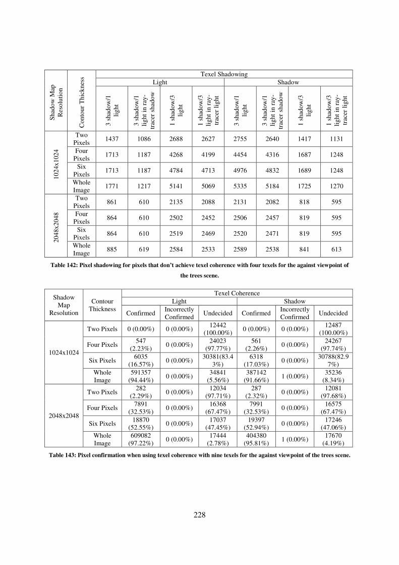
228
Sh
ado
w M
ap
Res
olu
tio
n
Co
nto
ur
Th
ick
nes
s Texel Shadowing
Light Shadow
3 s
had
ow
/1
lig
ht
3 s
had
ow
/1
lig
ht
in r
ay-
trac
er s
had
ow
1 s
had
ow
/3
lig
ht
1 s
had
ow
/3
lig
ht
in r
ay-
trac
er l
igh
t
3 s
had
ow
/1
lig
ht
3 s
had
ow
/1
lig
ht
in r
ay-
trac
er s
had
ow
1 s
had
ow
/3
lig
ht
1 s
had
ow
/3
lig
ht
in r
ay-
trac
er l
igh
t
10
24x
102
4
Two
Pixels 1437 1086 2688 2627 2755 2640 1417 1131
Four
Pixels 1713 1187 4268 4199 4454 4316 1687 1248
Six
Pixels 1713 1187 4784 4713 4976 4832 1689 1248
Whole
Image 1771 1217 5141 5069 5335 5184 1725 1270
20
48x
204
8
Two
Pixels 861 610 2135 2088 2131 2082 818 595
Four
Pixels 864 610 2502 2452 2506 2457 819 595
Six
Pixels 864 610 2519 2469 2520 2471 819 595
Whole
Image 885 619 2584 2533 2589 2538 841 613
Table 142: Pixel shadowing for pixels that don’t achieve texel coherence with four texels for the against viewpoint of
the trees scene.
Shadow
Map
Resolution
Contour
Thickness
Texel Coherence
Light Shadow
Confirmed Incorrectly
Confirmed Undecided Confirmed
Incorrectly
Confirmed Undecided
1024x1024
Two Pixels 0 (0.00%) 0 (0.00%) 12442
(100.00%) 0 (0.00%) 0 (0.00%)
12487
(100.00%)
Four Pixels 547
(2.23%) 0 (0.00%)
24023
(97.77%)
561
(2.26%) 0 (0.00%)
24267
(97.74%)
Six Pixels 6035
(16.57%) 0 (0.00%)
30381(83.4
3%)
6318
(17.03%) 0 (0.00%)
30788(82.9
7%)
Whole
Image
591357
(94.44%) 0 (0.00%)
34841
(5.56%)
387142
(91.66%) 1 (0.00%)
35236
(8.34%)
2048x2048
Two Pixels 282
(2.29%) 0 (0.00%)
12034
(97.71%)
287
(2.32%) 0 (0.00%)
12081
(97.68%)
Four Pixels 7891
(32.53%) 0 (0.00%)
16368
(67.47%)
7991
(32.53%) 0 (0.00%)
16575
(67.47%)
Six Pixels 18870
(52.55%) 0 (0.00%)
17037
(47.45%)
19397
(52.94%) 0 (0.00%)
17246
(47.06%)
Whole
Image
609082
(97.22%) 0 (0.00%)
17444
(2.78%)
404380
(95.81%) 1 (0.00%)
17670
(4.19%)
Table 143: Pixel confirmation when using texel coherence with nine texels for the against viewpoint of the trees scene.
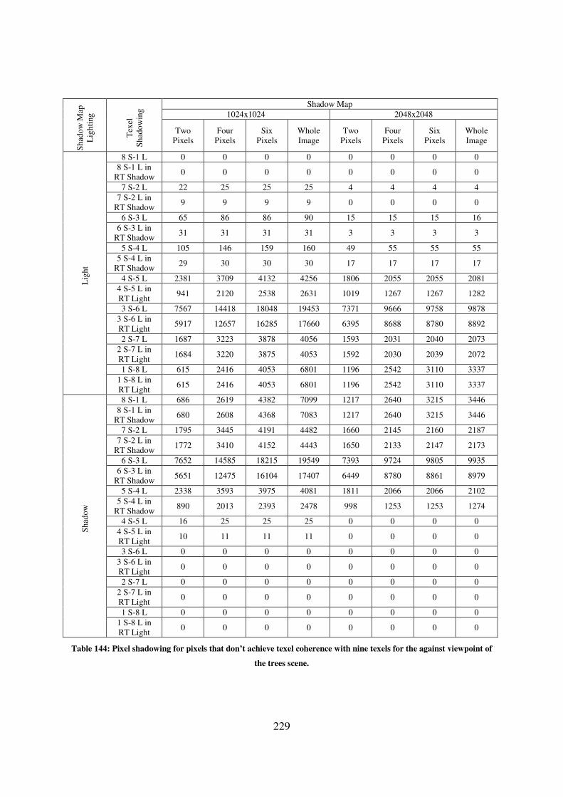
229
Sh
ado
w M
ap
Lig
hti
ng
Tex
el
Sh
ado
win
g Shadow Map
1024x1024 2048x2048
Two
Pixels
Four
Pixels
Six
Pixels
Whole
Image
Two
Pixels
Four
Pixels
Six
Pixels
Whole
Image
Lig
ht
8 S-1 L 0 0 0 0 0 0 0 0
8 S-1 L in
RT Shadow 0 0 0 0 0 0 0 0
7 S-2 L 22 25 25 25 4 4 4 4
7 S-2 L in
RT Shadow 9 9 9 9 0 0 0 0
6 S-3 L 65 86 86 90 15 15 15 16
6 S-3 L in
RT Shadow 31 31 31 31 3 3 3 3
5 S-4 L 105 146 159 160 49 55 55 55
5 S-4 L in
RT Shadow 29 30 30 30 17 17 17 17
4 S-5 L 2381 3709 4132 4256 1806 2055 2055 2081
4 S-5 L in
RT Light 941 2120 2538 2631 1019 1267 1267 1282
3 S-6 L 7567 14418 18048 19453 7371 9666 9758 9878
3 S-6 L in
RT Light 5917 12657 16285 17660 6395 8688 8780 8892
2 S-7 L 1687 3223 3878 4056 1593 2031 2040 2073
2 S-7 L in
RT Light 1684 3220 3875 4053 1592 2030 2039 2072
1 S-8 L 615 2416 4053 6801 1196 2542 3110 3337
1 S-8 L in
RT Light 615 2416 4053 6801 1196 2542 3110 3337
Sh
ado
w
8 S-1 L 686 2619 4382 7099 1217 2640 3215 3446
8 S-1 L in
RT Shadow 680 2608 4368 7083 1217 2640 3215 3446
7 S-2 L 1795 3445 4191 4482 1660 2145 2160 2187
7 S-2 L in
RT Shadow 1772 3410 4152 4443 1650 2133 2147 2173
6 S-3 L 7652 14585 18215 19549 7393 9724 9805 9935
6 S-3 L in
RT Shadow 5651 12475 16104 17407 6449 8780 8861 8979
5 S-4 L 2338 3593 3975 4081 1811 2066 2066 2102
5 S-4 L in
RT Shadow 890 2013 2393 2478 998 1253 1253 1274
4 S-5 L 16 25 25 25 0 0 0 0
4 S-5 L in
RT Light 10 11 11 11 0 0 0 0
3 S-6 L 0 0 0 0 0 0 0 0
3 S-6 L in
RT Light 0 0 0 0 0 0 0 0
2 S-7 L 0 0 0 0 0 0 0 0
2 S-7 L in
RT Light 0 0 0 0 0 0 0 0
1 S-8 L 0 0 0 0 0 0 0 0
1 S-8 L in
RT Light 0 0 0 0 0 0 0 0
Table 144: Pixel shadowing for pixels that don’t achieve texel coherence with nine texels for the against viewpoint of
the trees scene.

230
Shadow Map
Resolution
Contour
Thickness
Corrected Turned Bad Maintained Correct Maintained
Incorrect
L→S S→L L→S S→L L→L S→S L→L S→S
1024x1024
Two Pixels 0 3488 0 430 9280 8569 3162 0
Four Pixels 0 3747 0 838 21147 20243 3423 0
Six Pixels 0 3757 0 1437 32986 31912 3430 0
Whole Image 0 3812 0 17701 622707 400865 3491 0
2048x2048
Two Pixels 1 1767 0 216 10532 10385 1783 0
Four Pixels 1 1769 0 526 22472 22271 1786 0
Six Pixels 1 1770 0 877 34120 33996 1786 0
Whole Image 1 1799 0 9014 624720 411237 1805 0
Table 145: Pixel correction between the single texel approach and the shadow mapping approach for the against
viewpoint of the trees scene.
Shadow Map
Resolution
Contour
Thickness
Corrected Turned Bad Maintained Correct Maintained
Incorrect
L→S S→L L→S S→L L→L S→S L→L S→S
1024x1024
Two Pixels 2973 3488 0 198 9280 8801 189 0
Four Pixels 3212 3747 0 254 21147 20827 211 0
Six Pixels 3219 3757 0 332 32986 33017 211 0
Whole Image 3280 3812 0 1004 622707 417562 211 0
2048x2048
Two Pixels 1729 1767 0 64 10532 10537 55 0
Four Pixels 1732 1769 0 77 22472 22720 55 0
Six Pixels 1732 1770 0 97 34120 34776 55 0
Whole Image 1751 1799 0 234 624720 420017 55 0
Table 146: Pixel correction between the neighbour texels approach using four neighbours and the shadow mapping
approach for the against viewpoint of the trees scene.
Shadow Map
Resolution
Contour
Thickness
Corrected Turned Bad Maintained Correct Maintained
Incorrect
L→S S→L L→S S→L L→L S→S L→L S→S
1024x1024
Two Pixels 3055 3488 0 117 9280 8882 107 0
Four Pixels 3306 3747 0 152 21147 20929 117 0
Six Pixels 3313 3757 0 196 32986 33153 117 0
Whole Image 3374 3812 0 656 622707 417910 117 0
2048x2048
Two Pixels 1752 1767 0 37 10532 10564 32 0
Four Pixels 1755 1769 0 42 22472 22755 32 0
Six Pixels 1755 1770 0 52 34120 34821 32 0
Whole Image 1774 1799 0 146 624720 420105 32 0
Table 147: Pixel correction between the neighbour texels approach using nine neighbours and the shadow mapping
approach for the against viewpoint of the trees scene.

231
Sh
ado
w M
ap
Res
olu
tio
n
Nu
mb
er o
f
Nei
gh
bo
urs
Tri
ang
le
Av
erag
e
Two Pixels Four Pixels Six Pixels Whole Image
10
24x
102
4
3 Used 1.0563 0.9171 0.8294 0.5056
Available 1.0692 1.1000 1.1277 1.2053
8 Used 1.2201 1.2047 1.1357 0.6128
Available 1.2201 1.2182 1.2372 1.4055
20
48x
204
8
3 Used 0.8771 0.7322 0.6813 0.4552
Available 1.0503 1.0759 1.0906 1.1078
8 Used 1.0996 0.9549 0.8598 0.5088
Available 1.1124 1.1390 1.1620 1.1240
Table 148: Average of triangle intersections when using the neighbour texels approach for the against viewpoint of
the trees scene.
Shadow Map
Resolution
Contour
Thickness
Corrected Turned Bad Maintained Correct Maintained
Incorrect
L→S S→L L→S S→L L→L S→S L→L S→S
1024x1024
Two Pixels 0 3488 0 73 9280 8926 3162 0
Four Pixels 0 3747 0 116 21147 20965 3423 0
Six Pixels 0 3757 0 178 32986 33171 3430 0
Whole Image 0 3812 0 1488 622707 417078 3491 0
2048x2048
Two Pixels 1 1767 0 33 10532 10568 1783 0
Four Pixels 1 1769 0 54 22472 22743 1786 0
Six Pixels 1 1770 0 84 34120 34789 1786 0
Whole Image 1 1799 0 703 624720 419548 1805 0
Table 149: Pixel correction between the adjacent geometry approach with one level of adjacency and the shadow
mapping approach for the against viewpoint of the trees scene.
Shadow Map
Resolution
Contour
Thickness
Corrected Turned Bad Maintained Correct Maintained
Incorrect
L→S S→L L→S S→L L→L S→S L→L S→S
1024x1024
Two Pixels 0 3488 0 31 9280 8968 3162 0
Four Pixels 0 3747 0 46 21147 21035 3423 0
Six Pixels 0 3757 0 68 32986 33281 3430 0
Whole Image 0 3812 0 1092 622707 417474 3491 0
2048x2048
Two Pixels 1 1767 0 23 10532 10578 1783 0
Four Pixels 1 1769 0 28 22472 22769 1786 0
Six Pixels 1 1770 0 36 34120 34837 1786 0
Whole Image 1 1799 0 573 624720 419678 1805 0
Table 150: Pixel correction between the adjacent geometry approach with two level of adjacency and the shadow
mapping approach for the against viewpoint of the trees scene.

232
Sh
ado
w M
ap
Res
olu
tio
n
Ad
jace
ncy
Lev
el
Tri
ang
le
Av
erag
e
Two Pixels Four Pixels Six Pixels Whole Image
10
24x
102
4
One
Level
Used 2.0036 2.0104 2.0188 1.6112
Available 4.0000 4.0000 4.0000 4.0000
Two
Levels
Used 7.2241 7.2513 7.2870 5.8435
Available 14.4222 14.4273 14.4386 14.5067
20
48x
204
8
One
Level
Used 2.0042 2.0126 2.0203 1.6100
Available 4.0000 4.0000 4.0000 4.0000
Two
Levels
Used 7.2170 7.2547 7.2928 5.8400
Available 14.4036 14.4187 14.4392 14.5093
Table 151: Average of triangle intersections when using the adjacent geometry approach for the against viewpoint of
the trees scene.
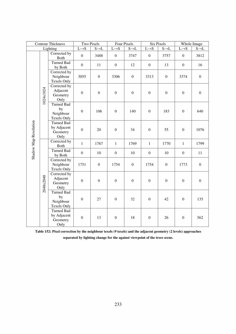
233
Contour Thickness Two Pixels Four Pixels Six Pixels Whole Image
Lighting L→S S→L L→S S→L L→S S→L L→S S→L
Sh
ado
w M
ap R
eso
luti
on
10
24x
102
4
Corrected by
Both 0 3488 0 3747 0 3757 0 3812
Turned Bad
by Both 0 11 0 12 0 13 0 16
Corrected by
Neighbour
Texels Only
3055 0 3306 0 3313 0 3374 0
Corrected by
Adjacent
Geometry
Only
0 0 0 0 0 0 0 0
Turned Bad
by
Neighbour
Texels Only
0 106 0 140 0 183 0 640
Turned Bad
by Adjacent
Geometry
Only
0 20 0 34 0 55 0 1076
20
48x
204
8
Corrected by
Both 1 1767 1 1769 1 1770 1 1799
Turned Bad
by Both 0 10 0 10 0 10 0 11
Corrected by
Neighbour
Texels Only
1751 0 1754 0 1754 0 1773 0
Corrected by
Adjacent
Geometry
Only
0 0 0 0 0 0 0 0
Turned Bad
by
Neighbour
Texels Only
0 27 0 32 0 42 0 135
Turned Bad
by Adjacent
Geometry
Only
0 13 0 18 0 26 0 562
Table 152: Pixel correction by the neighbour texels (9 texels) and the adjacent geometry (2 levels) approaches
separated by lighting change for the against viewpoint of the trees scene.

234
Alg
ori
thm
Ste
p
Confirmations
and Errors
1024x1024 2048x2048
Two Pixels Four Pixels Six Pixel Two Pixels Four Pixels Six Pixel
Sh
ado
w M
ap
Total Contour
Pixels 24929 49398 73522 24684 48825 72550
Correct Light
Pixels
9280
(74.59%)
21147
(86.07%)
32986
(90.58%)
10532
(85.51%)
22472
(92.63%)
34120
(95.02%)
Correct Shadow
Pixels
8999
(72.07%)
21081
(84.91%)
33349
(89.87%)
10601
(85.71%)
22797
(92.80%)
34873
(95.17%)
Incorrect Light
Pixels
3162
(25.41%)
3423
(13.93%)
3430
(9.42%)
1784
(14.49%)
1787
(7.37%)
1787
(4.98%)
Incorrect Shadow
Pixels
3488
(27.93%)
3747
(15.09%)
3757
(10.13%)
1767
(14.29%)
1769
(7.20%)
1770
(4.83%)
Tex
el C
oh
eren
ce
Confirmations in
Light
301
(2.42%)
8210
(33.41%)
19449
(53.41%)
4070
(33.05%)
15594
(64.28%)
27225
(75.82%)
Confirmations in
Shadow
296
(2.37%)
8302
(33.44%)
19976
(53.83%)
4175
(33.76%)
15955
(64.95%)
28018
(76.46%)
Wrong
Confirmations in
Light
0 (0.00%) 0 (0.00%) 0 (0.00%) 0 (0.00%) 0 (0.00%) 0 (0.00%)
Wrong
Confirmations in
Shadow
0 (0.00%) 2 (0.01%) 3 (0.01%) 0 (0.00%) 0 (0.00%) 1 (0.00%)
Nei
gh
bo
uri
ng
Tex
els
Corrections in
Light
3055
(24.55%)
3306
(13.46%)
3313
(9.10%)
1752
(14.23%)
1755
(7.23%)
1755
(4.89%)
Confirmations in
Shadow
8882
(71.13%)
20945
(84.36%)
33210
(89.50%)
10564
(85.41%)
22760
(92.65%)
34837
(95.07%)
Ad
jace
nt
Geo
met
ry
Confirmations in
Shadow
8988
(71.98%)
21072
(84.87%)
33341
(89.85%)
10591
(85.63%)
22787
(92.76%)
24864
(95.15%)
Fin
al L
igh
tin
g Wrong
Confirmations in
Light
107
(0.86%)
117
(0.48%)
117
(0.32%) 32 (0.26%) 32 (0.13%) 32 (0.09%)
Wrong
Confirmations in
Shadow
11 (0.09%) 13 (0.05%) 14 (0.04%) 10 (0.08%) 10 (0.04%) 11 (0.03%)
Table 153: Algorithm results of the against viewpoint of the trees scene.
And following below are the results of the “side” viewpoint of the “flowers” scene.
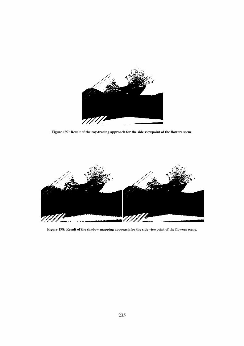
Figure 197: Result of the ray
Figure 198: Result of the shadow mapping approach for the
235
: Result of the ray-tracing approach for the side viewpoint of the flowers scene.
: Result of the shadow mapping approach for the side viewpoint of the flowers
tracing approach for the side viewpoint of the flowers scene.
flowers scene.
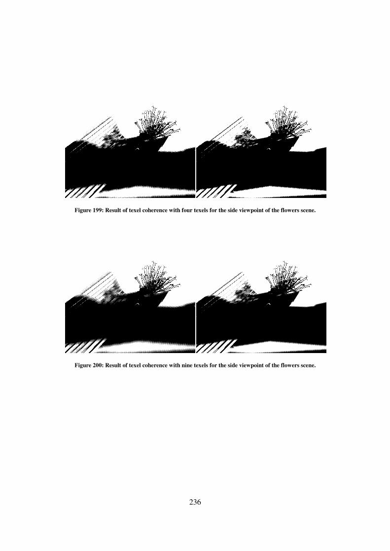
Figure 199: Result of texel coherence with four texels for
Figure 200: Result of texel coherence with nine texels for
236
: Result of texel coherence with four texels for the side viewpoint of the flowers scene
ult of texel coherence with nine texels for the side viewpoint of the flowers scene
the side viewpoint of the flowers scene.
the side viewpoint of the flowers scene.

237
Figure 201: Result of the single texel approach for the side viewpoint of the flowers scene.
Figure 202: Result of the neighbour texels approach using four neighbours for the side viewpoint of the flowers scene.
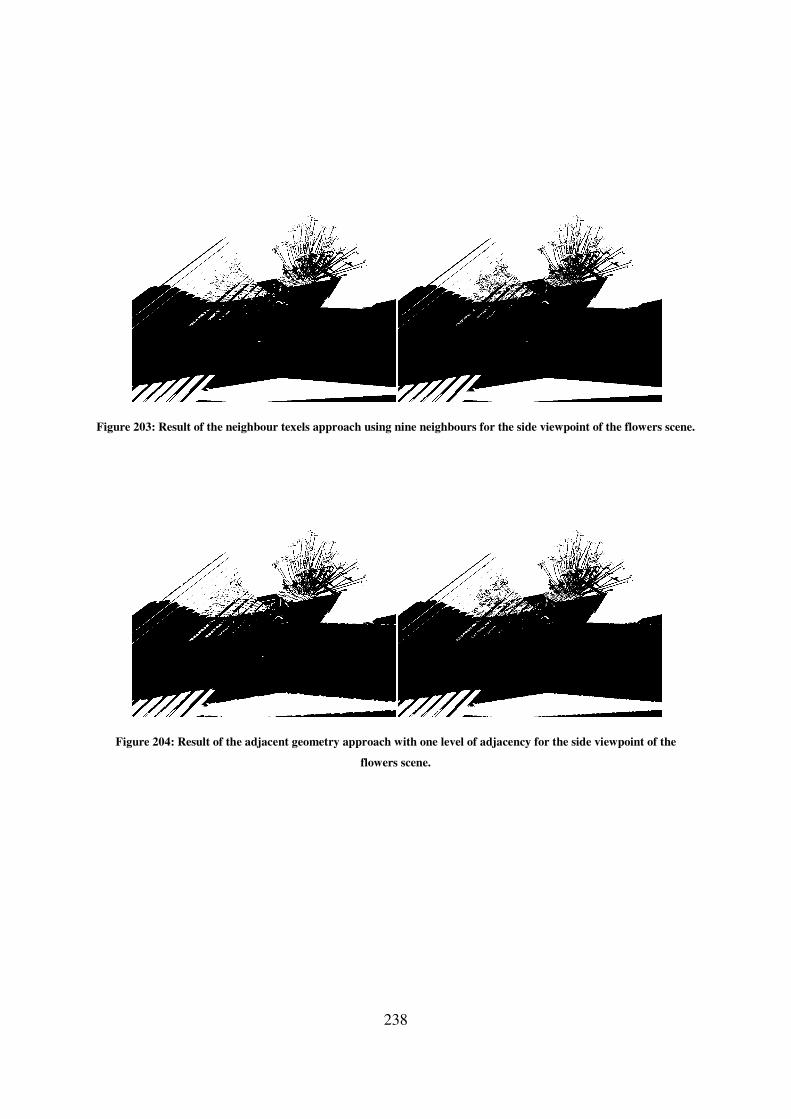
238
Figure 203: Result of the neighbour texels approach using nine neighbours for the side viewpoint of the flowers scene.
Figure 204: Result of the adjacent geometry approach with one level of adjacency for the side viewpoint of the
flowers scene.
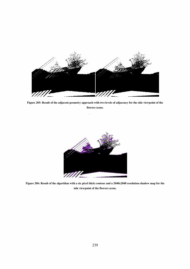
Figure 205: Result of the adjacent geometry
Figure 206: Result of the algorithm with a six pixel thick contour and a 2048x2048 resolution shadow map for the
239
adjacent geometry approach with two levels of adjacency for the side viewpoint of the
flowers scene.
: Result of the algorithm with a six pixel thick contour and a 2048x2048 resolution shadow map for the
side viewpoint of the flowers scene.
the side viewpoint of the
: Result of the algorithm with a six pixel thick contour and a 2048x2048 resolution shadow map for the
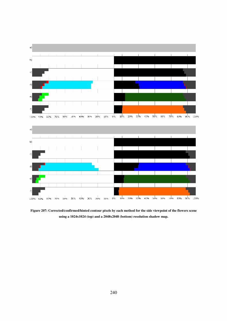
240
Figure 207: Corrected/confirmed/hinted contour pixels by each method for the side viewpoint of the flowers scene
using a 1024x1024 (top) and a 2048x2048 (bottom) resolution shadow map.
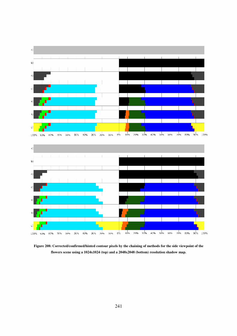
241
Figure 208: Corrected/confirmed/hinted contour pixels by the chaining of methods for the side viewpoint of the
flowers scene using a 1024x1024 (top) and a 2048x2048 (bottom) resolution shadow map.

242
Shadow Map
Resolution Approach
Contour Thickness
Two Pixels Four Pixels Six Pixels Whole Image
1024x1024
Pixels in
Contour 47368 80814 106784 1048576
Shadow Map 8434 (17.81%) 11724 (14.51%) 12834 (12.02%) 14226 (1.36%)
Single Texel 8486 (17.92%) 12690 (15.70%) 15046 (14.09%) 35332 (3.37%)
Neighbour
Texels (4
Neighbours)
6287 (13.27%) 9444 (11.69%) 11295 (10.58%) 21596 (2.06%)
Neighbour
Texels (9
Neighbours)
6015 (12.70%) 8994 (11.13%) 10793 (10.11%) 19922 (1.90%)
Adjacent
Geometry (One
Level)
7785 (16.44%) 11410 (14.12%) 13259 (12.42%) 23940 (2.28%)
Adjacent
Geometry
(Two Level)
7067 (14.92%) 10156 (12.57%) 11546 (10.81%) 19721 (1.88%)
2048x2048
Pixels in
Contour 49049 81863 106977 1048576
Shadow Map 6923 (14.11%) 7825 (9.56%) 8049 (7.52%) 8547 (0.82%)
Single Texel 8079 (16.47%) 10915 (13.33%) 12794 (11.96%) 26177 (2.50%)
Neighbour
Texels (4
Neighbours)
5775 (11.77%) 7881 (9.63%) 9325 (8.72%) 16347 (1.56%)
Neighbour
Texels (9
Neighbours)
5091 (10.38%) 6926 (8.46%) 8180 (7.65%) 13796 (1.32%)
Adjacent
Geometry (One
Level)
6745 (13.75%) 8570 (10.47%) 9834 (9.19%) 16461 (1.57%)
Adjacent
Geometry
(Two Level)
5259 (10.72%) 6345 (7.75%) 7041 (6.58%) 10510 (1.00%)
Table 154: Difference between the approaches that use ray-tracing and the actual ray-tracer for the side viewpoint of
the flowers scene.
Shadow Map Resolution Contour Thickness
Two Pixels Four Pixels Six Pixels
1024x1024 8434 of 14226 (59.29%) 11724 of 14226 (82.41%) 12834 of 14226 (90.22%)
2048x2048 6923 of 8547 (81.00%) 7825 of 8547 (91.55%) 8049 of 8547 (94.17%)
Table 155: Wrongly defined pixels in the shadow mapping result which are inside the contour in the side viewpoint of
the flowers scene.

243
Shadow Map Resolution Contour Thickness Pixel Shading
Light Shadow
1024x1024
Two Pixels 4866 of 24534 3568 of 22834
Four Pixels 6604 of 43942 5120 of 36872
Six Pixels 7144 of 59487 5690 of 47297
Whole Image 7550 of 639660 6676 of 408916
2048x2048
Two Pixels 3967 of 25180 2956 of 23869
Four Pixels 4422 of 43927 3403 of 37936
Six Pixels 4485 of 58619 3564 of 48358
Whole Image 4634 of 639507 3913 of 409069
Table 156: Pixels that the shadow map defines wrongly in the side viewpoint of the flowers scene, separated in pixels
defined in light and in shadow, compared to the total amount of pixels lighted in the same way.
Shadow
Map
Resolution
Contour
Thickness
Texel Coherence
Light Shadow
Confirmed Incorrectly
Confirmed Undecided Confirmed
Incorrectly
Confirmed Undecided
1024x1024
Two Pixels 13931
(56.78%)
642
(2.62%)
10603
(43.22%)
13402
(58.69%) 39 (0.17%)
9432
(41.31%)
Four Pixels 25723
(58.54%)
773
(1.76%)
18219
(41.46%)
20682
(56.09%) 81 (0.22%)
16190
(43.91%)
Six Pixels 36427
(61.24%)
825
(1.39%)
23060
(38.76%)
26880
(56.83%)
144
(0.30%)
20417
(43.17%)
Whole
Image
612550
(95.76%)
956
(0.15%)
27110
(4.24%)
384379
(94.00%)
787
(0.19%)
24537
(6.00%)
2048x2048
Two Pixels 14763
(58.63%)
389
(1.54%)
10417
(41.37%)
13648
(57.18%) 17 (0.07%)
10221
(42.82%)
Four Pixels 29524
(67.21%)
500
(1.14%)
14403
(32.79%)
23479
(61.89%)
125
(0.33%)
14457
(38.11%)
Six Pixels 43425
(74.08%)
543
(0.93%)
15194
(25.92%)
32922
(68.08%)
234
(0.48%)
15436
(31.92%)
Whole
Image
623784
(97.54%)
633
(0.10%)
15723
(2.46%)
392923
(96.05%)
498
(0.12%)
16146
(3.95%)
Table 157: Pixel confirmation when using texel coherence with four texels for the side viewpoint of the flowers scene.
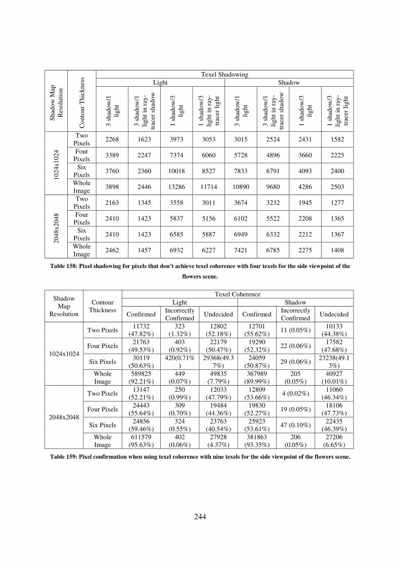
244
Sh
ado
w M
ap
Res
olu
tio
n
Co
nto
ur
Th
ick
nes
s Texel Shadowing
Light Shadow
3 s
had
ow
/1
lig
ht
3 s
had
ow
/1
lig
ht
in r
ay-
trac
er s
had
ow
1 s
had
ow
/3
lig
ht
1 s
had
ow
/3
lig
ht
in r
ay-
trac
er l
igh
t
3 s
had
ow
/1
lig
ht
3 s
had
ow
/1
lig
ht
in r
ay-
trac
er s
had
ow
1 s
had
ow
/3
lig
ht
1 s
had
ow
/3
lig
ht
in r
ay-
trac
er l
igh
t
10
24x
102
4
Two
Pixels 2268 1623 3973 3053 3015 2524 2431 1582
Four
Pixels 3389 2247 7374 6060 5728 4896 3660 2225
Six
Pixels 3760 2360 10018 8527 7833 6791 4093 2400
Whole
Image 3898 2446 13286 11714 10890 9680 4286 2503
20
48x
204
8
Two
Pixels 2163 1345 3558 3011 3674 3232 1945 1277
Four
Pixels 2410 1423 5837 5156 6102 5522 2208 1365
Six
Pixels 2410 1423 6585 5887 6949 6332 2212 1367
Whole
Image 2462 1457 6932 6227 7421 6785 2275 1408
Table 158: Pixel shadowing for pixels that don’t achieve texel coherence with four texels for the side viewpoint of the
flowers scene.
Shadow
Map
Resolution
Contour
Thickness
Texel Coherence
Light Shadow
Confirmed Incorrectly
Confirmed Undecided Confirmed
Incorrectly
Confirmed Undecided
1024x1024
Two Pixels 11732
(47.82%)
323
(1.32%)
12802
(52.18%)
12701
(55.62%) 11 (0.05%)
10133
(44.38%)
Four Pixels 21763
(49.53%)
403
(0.92%)
22179
(50.47%)
19290
(52.32%) 22 (0.06%)
17582
(47.68%)
Six Pixels 30119
(50.63%)
420(0.71%
)
29368(49.3
7%)
24059
(50.87%) 29 (0.06%)
23238(49.1
3%)
Whole
Image
589825
(92.21%)
449
(0.07%)
49835
(7.79%)
367989
(89.99%)
205
(0.05%)
40927
(10.01%)
2048x2048
Two Pixels 13147
(52.21%)
250
(0.99%)
12033
(47.79%)
12809
(53.66%) 4 (0.02%)
11060
(46.34%)
Four Pixels 24443
(55.64%)
309
(0.70%)
19484
(44.36%)
19830
(52.27%) 19 (0.05%)
18106
(47.73%)
Six Pixels 24856
(59.46%)
324
(0.55%)
23763
(40.54%)
25923
(53.61%) 47 (0.10%)
22435
(46.39%)
Whole
Image
611579
(95.63%)
402
(0.06%)
27928
(4.37%)
381863
(93.35%)
206
(0.05%)
27206
(6.65%)
Table 159: Pixel confirmation when using texel coherence with nine texels for the side viewpoint of the flowers scene.
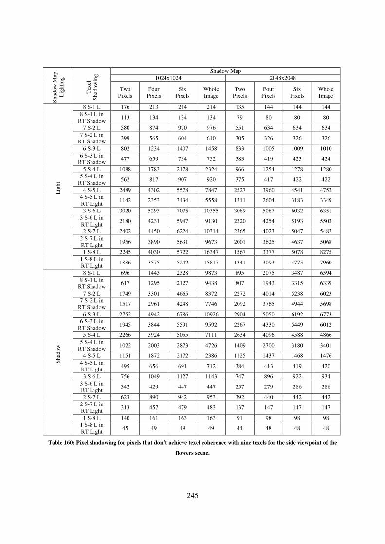
245
Sh
ado
w M
ap
Lig
hti
ng
Tex
el
Sh
ado
win
g Shadow Map
1024x1024 2048x2048
Two
Pixels
Four
Pixels
Six
Pixels
Whole
Image
Two
Pixels
Four
Pixels
Six
Pixels
Whole
Image
Lig
ht
8 S-1 L 176 213 214 214 135 144 144 144
8 S-1 L in
RT Shadow 113 134 134 134 79 80 80 80
7 S-2 L 580 874 970 976 551 634 634 634
7 S-2 L in
RT Shadow 399 565 604 610 305 326 326 326
6 S-3 L 802 1234 1407 1458 833 1005 1009 1010
6 S-3 L in
RT Shadow 477 659 734 752 383 419 423 424
5 S-4 L 1088 1783 2178 2324 966 1254 1278 1280
5 S-4 L in
RT Shadow 562 817 907 920 375 417 422 422
4 S-5 L 2489 4302 5578 7847 2527 3960 4541 4752
4 S-5 L in
RT Light 1142 2353 3434 5558 1311 2604 3183 3349
3 S-6 L 3020 5293 7075 10355 3089 5087 6032 6351
3 S-6 L in
RT Light 2180 4231 5947 9130 2320 4254 5193 5503
2 S-7 L 2402 4450 6224 10314 2365 4023 5047 5482
2 S-7 L in
RT Light 1956 3890 5631 9673 2001 3625 4637 5068
1 S-8 L 2245 4030 5722 16347 1567 3377 5078 8275
1 S-8 L in
RT Light 1886 3575 5242 15817 1341 3093 4775 7960
Sh
ado
w
8 S-1 L 696 1443 2328 9873 895 2075 3487 6594
8 S-1 L in
RT Shadow 617 1295 2127 9438 807 1943 3315 6339
7 S-2 L 1749 3301 4665 8372 2272 4014 5238 6023
7 S-2 L in
RT Shadow 1517 2961 4248 7746 2092 3765 4944 5698
6 S-3 L 2752 4942 6786 10926 2904 5050 6192 6773
6 S-3 L in
RT Shadow 1945 3844 5591 9592 2267 4330 5449 6012
5 S-4 L 2266 3924 5055 7111 2634 4096 4588 4866
5 S-4 L in
RT Shadow 1022 2003 2873 4726 1409 2700 3180 3401
4 S-5 L 1151 1872 2172 2386 1125 1437 1468 1476
4 S-5 L in
RT Light 495 656 691 712 384 413 419 420
3 S-6 L 756 1049 1127 1143 747 896 922 934
3 S-6 L in
RT Light 342 429 447 447 257 279 286 286
2 S-7 L 623 890 942 953 392 440 442 442
2 S-7 L in
RT Light 313 457 479 483 137 147 147 147
1 S-8 L 140 161 163 163 91 98 98 98
1 S-8 L in
RT Light 45 49 49 49 44 48 48 48
Table 160: Pixel shadowing for pixels that don’t achieve texel coherence with nine texels for the side viewpoint of the
flowers scene.
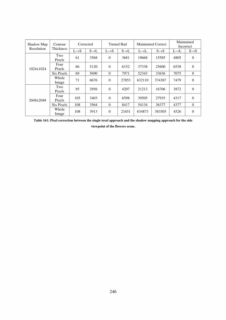
246
Shadow Map
Resolution
Contour
Thickness
Corrected Turned Bad Maintained Correct Maintained
Incorrect
L→S S→L L→S S→L L→L S→S L→L S→S
1024x1024
Two
Pixels 61 3568 0 3681 19668 15585 4805 0
Four
Pixels 66 5120 0 6152 37338 25600 6538 0
Six Pixels 69 5690 0 7971 52343 33636 7075 0
Whole
Image 71 6676 0 27853 632110 374387 7479 0
2048x2048
Two
Pixels 95 2956 0 4207 21213 16706 3872 0
Four
Pixels 105 3403 0 6598 39505 27935 4317 0
Six Pixels 108 3564 0 8417 54134 36377 4377 0
Whole
Image 108 3913 0 21651 634873 383505 4526 0
Table 161: Pixel correction between the single texel approach and the shadow mapping approach for the side
viewpoint of the flowers scene.
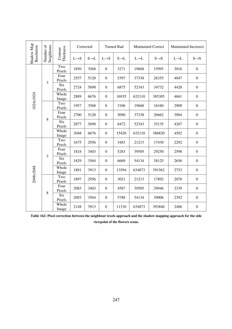
247
Sh
ado
w M
ap
Res
olu
tio
n
Nu
mb
er o
f
Nei
gh
bo
urs
Co
nto
ur
Th
ick
nes
s Corrected Turned Bad Maintained Correct Maintained Incorrect
L→S S→L L→S S→L L→L S→S L→L S→S
10
24x
102
4
3
Two
Pixels 1850 3568 0 3271 19668 15995 3016 0
Four
Pixels 2557 5120 0 5397 37338 26355 4047 0
Six
Pixels 2724 5690 0 6875 52343 34732 4420 0
Whole
Image 2889 6676 0 16935 632110 385305 4661 0
8
Two
Pixels 1957 3568 0 3106 19668 16160 2909 0
Four
Pixels 2700 5120 0 5090 37338 26662 3904 0
Six
Pixels 2877 5690 0 6472 52343 35135 4267 0
Whole
Image 3048 6676 0 15420 632110 386820 4502 0
20
48x
204
8
3
Two
Pixels 1675 2956 0 3483 21213 17430 2292 0
Four
Pixels 1824 3403 0 5283 39505 29250 2598 0
Six
Pixels 1829 3564 0 6669 54134 38125 2656 0
Whole
Image 1881 3913 0 13594 634873 391562 2753 0
8
Two
Pixels 1897 2956 0 3021 21213 17892 2070 0
Four
Pixels 2083 3403 0 4587 39505 29946 2339 0
Six
Pixels 2093 3564 0 5788 54134 39006 2392 0
Whole
Image 2148 3913 0 11310 634873 393846 2486 0
Table 162: Pixel correction between the neighbour texels approach and the shadow mapping approach for the side
viewpoint of the flowers scene.
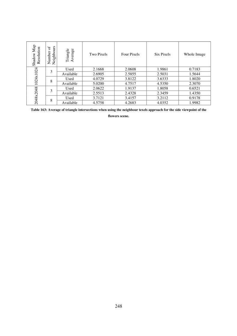
248
Sh
ado
w M
ap
Res
olu
tio
n
Nu
mb
er o
f
Nei
gh
bo
urs
Tri
ang
le
Av
erag
e
Two Pixels Four Pixels Six Pixels Whole Image
10
24x
102
4
3 Used 2.1668 2.0608 1.9861 0.7183
Available 2.6905 2.5855 2.5031 1.5644
8 Used 4.0729 3.8122 3.6333 1.8020
Available 5.0200 4.7517 4.5350 2.3070
20
48x
204
8
3 Used 2.0622 1.9137 1.8058 0.6521
Available 2.5513 2.4328 2.3459 1.4350
8 Used 3.7121 3.4157 3.2112 0.9178
Available 4.5758 4.2683 4.0352 1.9982
Table 163: Average of triangle intersections when using the neighbour texels approach for the side viewpoint of the
flowers scene.
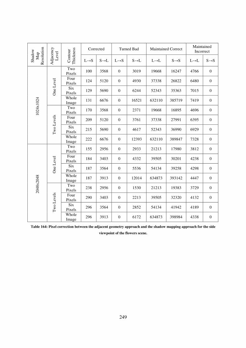
249
Sh
ado
w
Map
Res
olu
tio
n
Ad
jace
ncy
Lev
el
Co
nto
ur
Th
ick
nes
s Corrected Turned Bad Maintained Correct Maintained
Incorrect
L→S S→L L→S S→L L→L S→S L→L S→S
10
24x
102
4 O
ne
Lev
el
Two
Pixels 100 3568 0 3019 19668 16247 4766 0
Four
Pixels 124 5120 0 4930 37338 26822 6480 0
Six
Pixels 129 5690 0 6244 52343 35363 7015 0
Whole
Image 131 6676 0 16521 632110 385719 7419 0
Tw
o L
evel
s
Two
Pixels 170 3568 0 2371 19668 16895 4696 0
Four
Pixels 209 5120 0 3761 37338 27991 6395 0
Six
Pixels 215 5690 0 4617 52343 36990 6929 0
Whole
Image 222 6676 0 12393 632110 389847 7328 0
20
48x
204
8 O
ne
Lev
el
Two
Pixels 155 2956 0 2933 21213 17980 3812 0
Four
Pixels 184 3403 0 4332 39505 30201 4238 0
Six
Pixels 187 3564 0 5536 54134 39258 4298 0
Whole
Image 187 3913 0 12014 634873 393142 4447 0
Tw
o L
evel
s
Two
Pixels 238 2956 0 1530 21213 19383 3729 0
Four
Pixels 290 3403 0 2213 39505 32320 4132 0
Six
Pixels 296 3564 0 2852 54134 41942 4189 0
Whole
Image 296 3913 0 6172 634873 398984 4338 0
Table 164: Pixel correction between the adjacent geometry approach and the shadow mapping approach for the side
viewpoint of the flowers scene.

250
Sh
ado
w M
ap
Res
olu
tio
n
Ad
jace
ncy
Lev
el
Tri
ang
le
Av
erag
e
Two Pixels Four Pixels Six Pixels Whole Image
10
24x
102
4
One
Level
Used 2.7295 2.6990 2.6858 1.7635
Available 3.8489 3.8588 3.8681 3.9550
Two
Levels
Used 8.5830 8.4226 8.3134 5.7143
Available 12.1029 12.0421 11.9728 12.8153
20
48x
204
8
One
Level
Used 2.8069 2.7537 2.7375 1.7690
Available 3.8693 3.8748 3.8850 3.9583
Two
Levels
Used 9.0359 8.7366 8.6129 5.7363
Available 12.4558 12.2932 12.2235 12.8352
Table 165: Average of triangle intersections when using the adjacent geometry approach for the side viewpoint of the
flowers scene.

251
Contour Thickness Two Pixels Four Pixels Six Pixels Whole Image
Lighting L→S S→L L→S S→L L→S S→L L→S S→L
Sh
ado
w M
ap R
eso
luti
on
10
24x
102
4
Corrected by
Both 76 3568 82 5120 85 5690 87 6676
Turned Bad
by Both 0 2148 0 3355 0 4072 0 10147
Corrected by
Neighbour
Texels Only
1881 0 2618 0 2792 0 2961 0
Corrected by
Adjacent
Geometry
Only
94 0 127 0 130 0 135 0
Turned Bad
by
Neighbour
Texels Only
0 958 0 1735 0 2400 0 5273
Turned Bad
by Adjacent
Geometry
Only
0 223 0 406 0 545 0 2246
20
48x
204
8
Corrected by
Both 128 2956 146 3403 150 3564 150 3913
Turned Bad
by Both 0 1240 0 1753 0 2268 0 4596
Corrected by
Neighbour
Texels Only
1769 0 1937 0 1943 0 1998 0
Corrected by
Adjacent
Geometry
Only
110 0 144 0 146 0 146 0
Turned Bad
by
Neighbour
Texels Only
0 1781 0 2834 0 3520 0 6714
Turned Bad
by Adjacent
Geometry
Only
0 290 0 460 0 584 0 1576
Table 166: Pixel correction by the neighbour texels (9 texels) and the adjacent geometry (2 levels) approaches
separated by lighting change for the side viewpoint of the flowers scene.
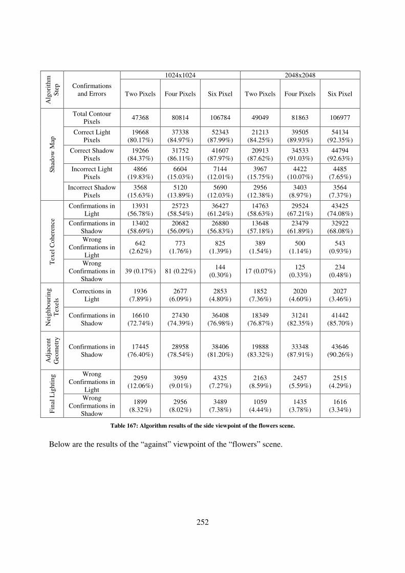
252
Alg
ori
thm
Ste
p
Confirmations
and Errors
1024x1024 2048x2048
Two Pixels Four Pixels Six Pixel Two Pixels Four Pixels Six Pixel
Sh
ado
w M
ap
Total Contour
Pixels 47368 80814 106784 49049 81863 106977
Correct Light
Pixels
19668
(80.17%)
37338
(84.97%)
52343
(87.99%)
21213
(84.25%)
39505
(89.93%)
54134
(92.35%)
Correct Shadow
Pixels
19266
(84.37%)
31752
(86.11%)
41607
(87.97%)
20913
(87.62%)
34533
(91.03%)
44794
(92.63%)
Incorrect Light
Pixels
4866
(19.83%)
6604
(15.03%)
7144
(12.01%)
3967
(15.75%)
4422
(10.07%)
4485
(7.65%)
Incorrect Shadow
Pixels
3568
(15.63%)
5120
(13.89%)
5690
(12.03%)
2956
(12.38%)
3403
(8.97%)
3564
(7.37%)
Tex
el C
oh
eren
ce
Confirmations in
Light
13931
(56.78%)
25723
(58.54%)
36427
(61.24%)
14763
(58.63%)
29524
(67.21%)
43425
(74.08%)
Confirmations in
Shadow
13402
(58.69%)
20682
(56.09%)
26880
(56.83%)
13648
(57.18%)
23479
(61.89%)
32922
(68.08%)
Wrong
Confirmations in
Light
642
(2.62%)
773
(1.76%)
825
(1.39%)
389
(1.54%)
500
(1.14%)
543
(0.93%)
Wrong
Confirmations in
Shadow
39 (0.17%) 81 (0.22%) 144
(0.30%) 17 (0.07%)
125
(0.33%)
234
(0.48%)
Nei
gh
bo
uri
ng
Tex
els
Corrections in
Light
1936
(7.89%)
2677
(6.09%)
2853
(4.80%)
1852
(7.36%)
2020
(4.60%)
2027
(3.46%)
Confirmations in
Shadow
16610
(72.74%)
27430
(74.39%)
36408
(76.98%)
18349
(76.87%)
31241
(82.35%)
41442
(85.70%)
Ad
jace
nt
Geo
met
ry
Confirmations in
Shadow
17445
(76.40%)
28958
(78.54%)
38406
(81.20%)
19888
(83.32%)
33348
(87.91%)
43646
(90.26%)
Fin
al L
igh
tin
g Wrong
Confirmations in
Light
2959
(12.06%)
3959
(9.01%)
4325
(7.27%)
2163
(8.59%)
2457
(5.59%)
2515
(4.29%)
Wrong
Confirmations in
Shadow
1899
(8.32%)
2956
(8.02%)
3489
(7.38%)
1059
(4.44%)
1435
(3.78%)
1616
(3.34%)
Table 167: Algorithm results of the side viewpoint of the flowers scene.
Below are the results of the “against” viewpoint of the “flowers” scene.
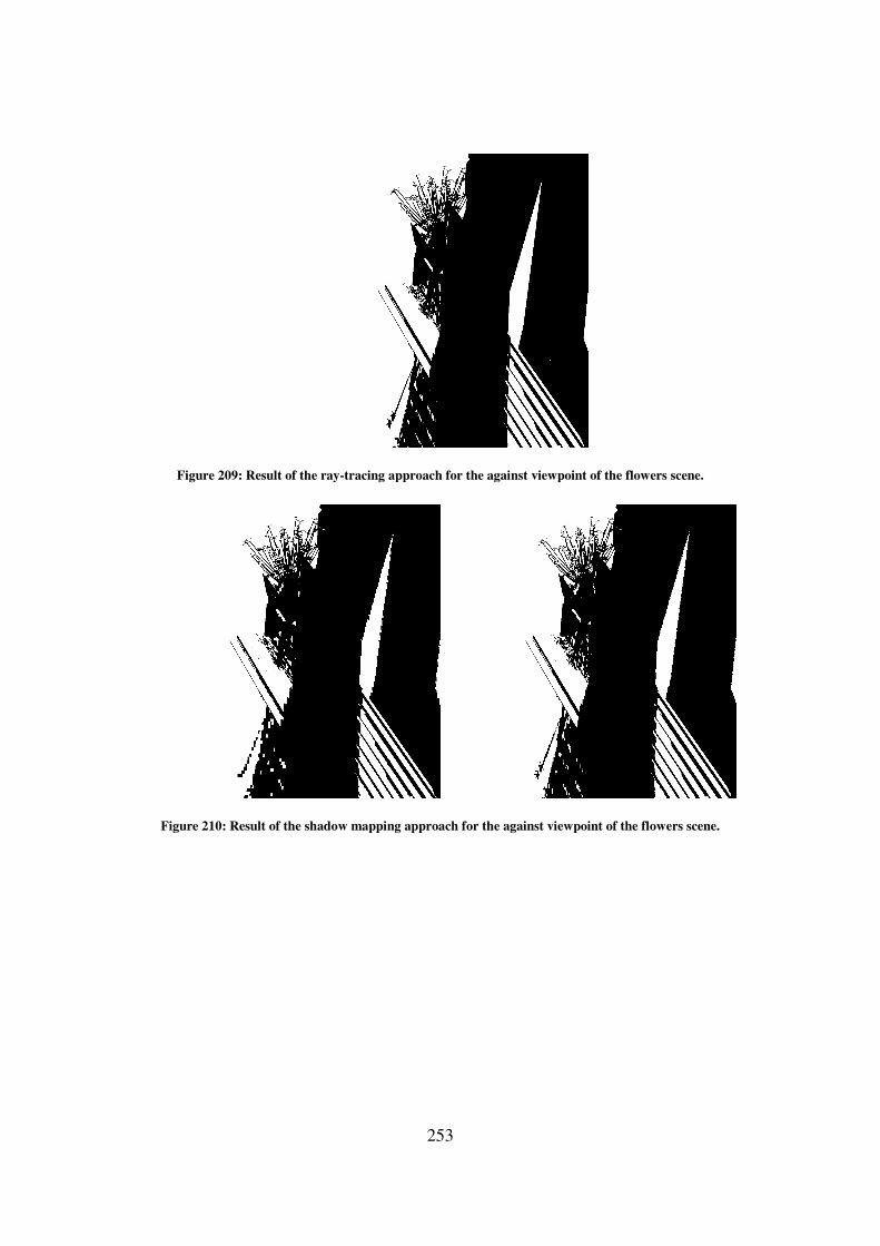
Figure 209: Result of the ray
Figure 210: Result of the shadow mapping approach for the
253
: Result of the ray-tracing approach for the against viewpoint of the flowers scene.
: Result of the shadow mapping approach for the against viewpoint of the
tracing approach for the against viewpoint of the flowers scene.
viewpoint of the flowers scene.
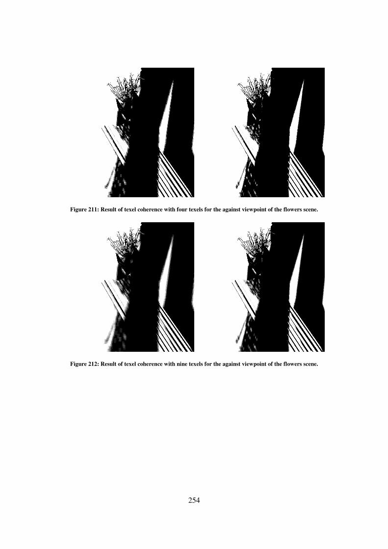
Figure 211: Result of texel coherence with four texels for
Figure 212: Result of texel coherence with nine texels for
254
: Result of texel coherence with four texels for the against viewpoint of the flowers scene
: Result of texel coherence with nine texels for the against viewpoint of the flowers scene
the against viewpoint of the flowers scene.
the against viewpoint of the flowers scene.
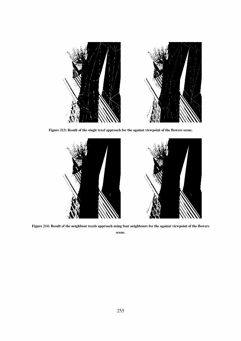
255
Figure 213: Result of the single texel approach for the against viewpoint of the flowers scene.
Figure 214: Result of the neighbour texels approach using four neighbours for the against viewpoint of the flowers
scene.
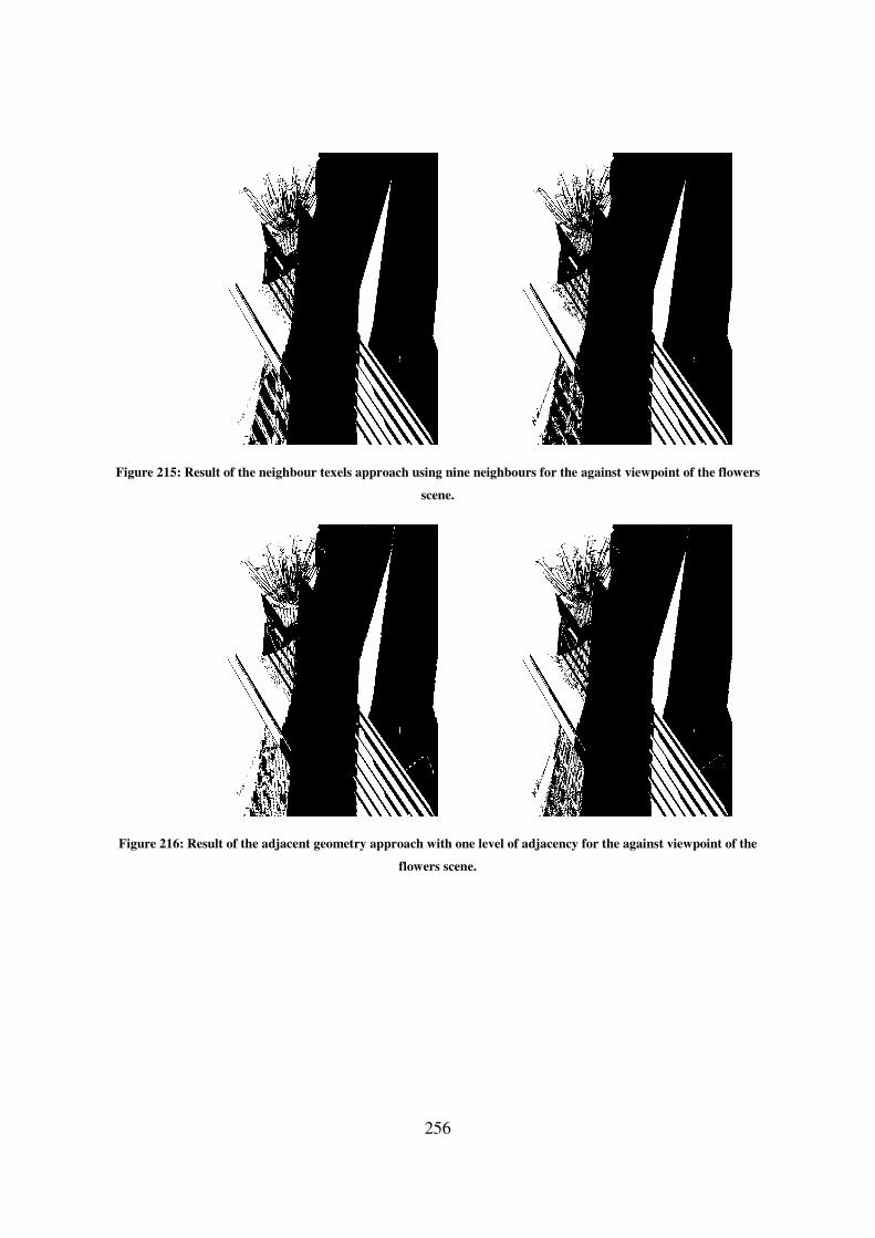
256
Figure 215: Result of the neighbour texels approach using nine neighbours for the against viewpoint of the flowers
scene.
Figure 216: Result of the adjacent geometry approach with one level of adjacency for the against viewpoint of the
flowers scene.
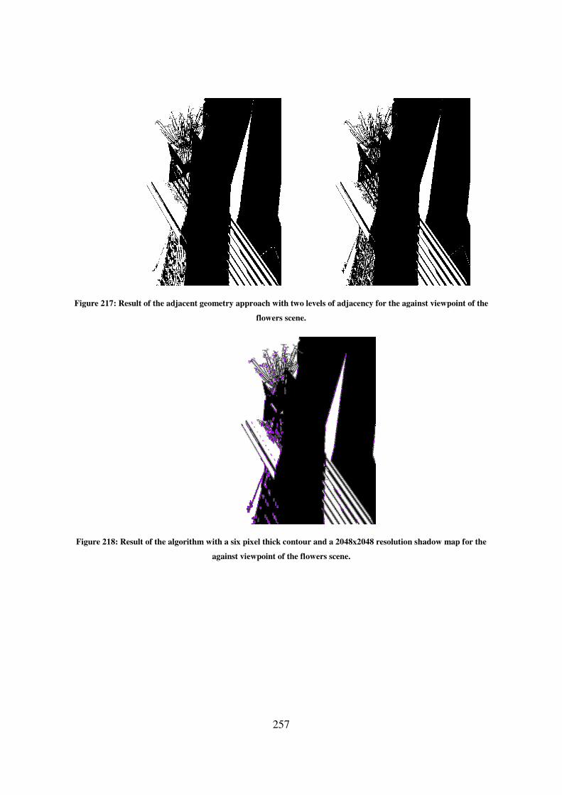
Figure 217: Result of the adjacent geometry
Figure 218: Result of the algorithm with a six pixel thick contour and a 2048x2048 resolution shadow map for the
257
adjacent geometry approach with two levels of adjacency for the against viewpoint of the
flowers scene.
: Result of the algorithm with a six pixel thick contour and a 2048x2048 resolution shadow map for the
against viewpoint of the flowers scene.
the against viewpoint of the
: Result of the algorithm with a six pixel thick contour and a 2048x2048 resolution shadow map for the

258
Figure 219: Corrected/confirmed/hinted contour pixels by each method for the against viewpoint of the flowers scene
using a 1024x1024 (top) and a 2048x2048 (bottom) resolution shadow map.
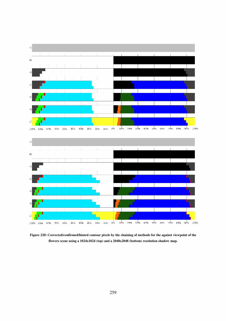
259
Figure 220: Corrected/confirmed/hinted contour pixels by the chaining of methods for the against viewpoint of the
flowers scene using a 1024x1024 (top) and a 2048x2048 (bottom) resolution shadow map.

260
Shadow Map
Resolution Approach
Contour Thickness
Two Pixels Four Pixels Six Pixels Whole Image
1024x1024
Pixels in
Contour 48869 85292 114428 1048576
Shadow Map 7239 (14.81%) 9885 (11.59%) 10649 (9.31%) 12037 (1.15%)
Single Texel 6915 (14.15%) 10756 (12.61%) 13139 (11.48%) 48387 (4.61%)
Neighbour
Texels (4
Neighbours)
4905 (10.04%) 7778 (9.12%) 9575 (8.37%) 26983 (2.57%)
Neighbour
Texels (9
Neighbours)
4545 (9.30%) 7165 (8.40%) 8755 (7.65%) 22720 (2.17%)
Adjacent
Geometry (One
Level)
6153 (12.59%) 9384 (11.00%) 11095 (9.70%) 32269 (3.08%)
Adjacent
Geometry
(Two Level)
5514 (11.28%) 8143 (9.55%) 9315 (8.14%) 25575 (2.44%)
2048x2048
Pixels in
Contour 51578 88386 117375 1048576
Shadow Map 6154 (11.93%) 6869 (7.77%) 7091 (6.04%) 7398 (0.71%)
Single Texel 7006 (13.58%) 9685 (10.96%) 12180 (10.38%) 35979 (3.43%)
Neighbour
Texels (4
Neighbours)
4727 (9.16%) 6511 (7.37%) 8109 (6.91%) 19187 (1.83%)
Neighbour
Texels (9
Neighbours)
3996 (7.75%) 5419 (6.13%) 6602 (5.62%) 14209 (1.36%)
Adjacent
Geometry (One
Level)
5776 (11.20%) 7335 (8.30%) 9128 (7.78%) 22385 (2.13%)
Adjacent
Geometry(Two
Level)
4581 (8.88%) 5461 (6.18%) 6502 (5.54%) 14343 (1.37%)
Table 168: Difference between the approaches that use ray-tracing and the actual ray-tracer for the against
viewpoint of the flowers scene.
Shadow Map Resolution Contour Thickness
Two Pixels Four Pixels Six Pixels
1024x1024 7239 of 12037 (60.14%) 9885 of 12037 (82.12%) 10649 of 12037 (88.47%)
2048x2048 6154 of 7398 (83.18%) 6869 of 7398 (92.85%) 7091 of 7398 (95.85%)
Table 169: Wrongly defined pixels in the shadow mapping result which are inside the contour in the against
viewpoint of the flowers scene.
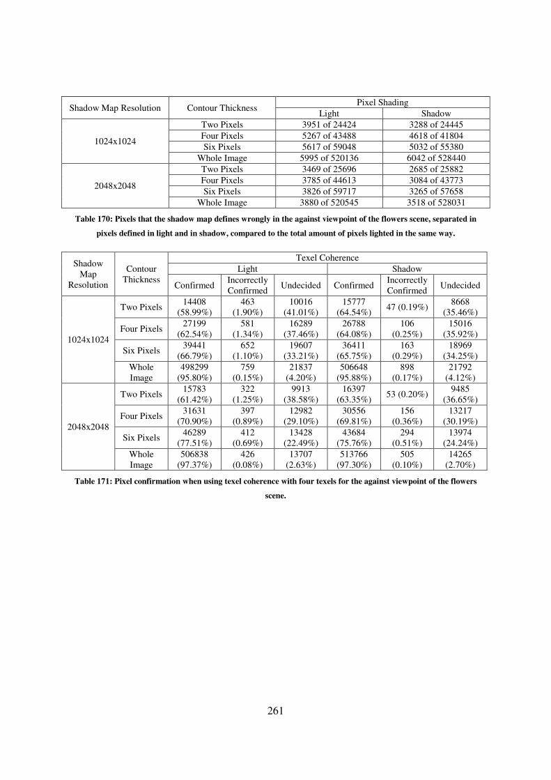
261
Shadow Map Resolution Contour Thickness Pixel Shading
Light Shadow
1024x1024
Two Pixels 3951 of 24424 3288 of 24445
Four Pixels 5267 of 43488 4618 of 41804
Six Pixels 5617 of 59048 5032 of 55380
Whole Image 5995 of 520136 6042 of 528440
2048x2048
Two Pixels 3469 of 25696 2685 of 25882
Four Pixels 3785 of 44613 3084 of 43773
Six Pixels 3826 of 59717 3265 of 57658
Whole Image 3880 of 520545 3518 of 528031
Table 170: Pixels that the shadow map defines wrongly in the against viewpoint of the flowers scene, separated in
pixels defined in light and in shadow, compared to the total amount of pixels lighted in the same way.
Shadow
Map
Resolution
Contour
Thickness
Texel Coherence
Light Shadow
Confirmed Incorrectly
Confirmed Undecided Confirmed
Incorrectly
Confirmed Undecided
1024x1024
Two Pixels 14408
(58.99%)
463
(1.90%)
10016
(41.01%)
15777
(64.54%) 47 (0.19%)
8668
(35.46%)
Four Pixels 27199
(62.54%)
581
(1.34%)
16289
(37.46%)
26788
(64.08%)
106
(0.25%)
15016
(35.92%)
Six Pixels 39441
(66.79%)
652
(1.10%)
19607
(33.21%)
36411
(65.75%)
163
(0.29%)
18969
(34.25%)
Whole
Image
498299
(95.80%)
759
(0.15%)
21837
(4.20%)
506648
(95.88%)
898
(0.17%)
21792
(4.12%)
2048x2048
Two Pixels 15783
(61.42%)
322
(1.25%)
9913
(38.58%)
16397
(63.35%) 53 (0.20%)
9485
(36.65%)
Four Pixels 31631
(70.90%)
397
(0.89%)
12982
(29.10%)
30556
(69.81%)
156
(0.36%)
13217
(30.19%)
Six Pixels 46289
(77.51%)
412
(0.69%)
13428
(22.49%)
43684
(75.76%)
294
(0.51%)
13974
(24.24%)
Whole
Image
506838
(97.37%)
426
(0.08%)
13707
(2.63%)
513766
(97.30%)
505
(0.10%)
14265
(2.70%)
Table 171: Pixel confirmation when using texel coherence with four texels for the against viewpoint of the flowers
scene.
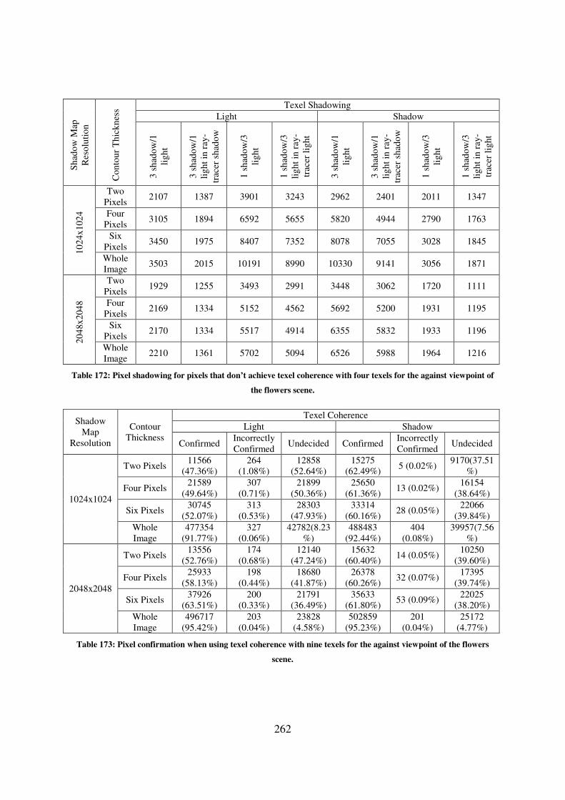
262
Sh
ado
w M
ap
Res
olu
tio
n
Co
nto
ur
Th
ick
nes
s Texel Shadowing
Light Shadow
3 s
had
ow
/1
lig
ht
3 s
had
ow
/1
lig
ht
in r
ay-
trac
er s
had
ow
1 s
had
ow
/3
lig
ht
1 s
had
ow
/3
lig
ht
in r
ay-
trac
er l
igh
t
3 s
had
ow
/1
lig
ht
3 s
had
ow
/1
lig
ht
in r
ay-
trac
er s
had
ow
1 s
had
ow
/3
lig
ht
1 s
had
ow
/3
lig
ht
in r
ay-
trac
er l
igh
t
10
24x
102
4
Two
Pixels 2107 1387 3901 3243 2962 2401 2011 1347
Four
Pixels 3105 1894 6592 5655 5820 4944 2790 1763
Six
Pixels 3450 1975 8407 7352 8078 7055 3028 1845
Whole
Image 3503 2015 10191 8990 10330 9141 3056 1871
20
48x
204
8
Two
Pixels 1929 1255 3493 2991 3448 3062 1720 1111
Four
Pixels 2169 1334 5152 4562 5692 5200 1931 1195
Six
Pixels 2170 1334 5517 4914 6355 5832 1933 1196
Whole
Image 2210 1361 5702 5094 6526 5988 1964 1216
Table 172: Pixel shadowing for pixels that don’t achieve texel coherence with four texels for the against viewpoint of
the flowers scene.
Shadow
Map
Resolution
Contour
Thickness
Texel Coherence
Light Shadow
Confirmed Incorrectly
Confirmed Undecided Confirmed
Incorrectly
Confirmed Undecided
1024x1024
Two Pixels 11566
(47.36%)
264
(1.08%)
12858
(52.64%)
15275
(62.49%) 5 (0.02%)
9170(37.51
%)
Four Pixels 21589
(49.64%)
307
(0.71%)
21899
(50.36%)
25650
(61.36%) 13 (0.02%)
16154
(38.64%)
Six Pixels 30745
(52.07%)
313
(0.53%)
28303
(47.93%)
33314
(60.16%) 28 (0.05%)
22066
(39.84%)
Whole
Image
477354
(91.77%)
327
(0.06%)
42782(8.23
%)
488483
(92.44%)
404
(0.08%)
39957(7.56
%)
2048x2048
Two Pixels 13556
(52.76%)
174
(0.68%)
12140
(47.24%)
15632
(60.40%) 14 (0.05%)
10250
(39.60%)
Four Pixels 25933
(58.13%)
198
(0.44%)
18680
(41.87%)
26378
(60.26%) 32 (0.07%)
17395
(39.74%)
Six Pixels 37926
(63.51%)
200
(0.33%)
21791
(36.49%)
35633
(61.80%) 53 (0.09%)
22025
(38.20%)
Whole
Image
496717
(95.42%)
203
(0.04%)
23828
(4.58%)
502859
(95.23%)
201
(0.04%)
25172
(4.77%)
Table 173: Pixel confirmation when using texel coherence with nine texels for the against viewpoint of the flowers
scene.
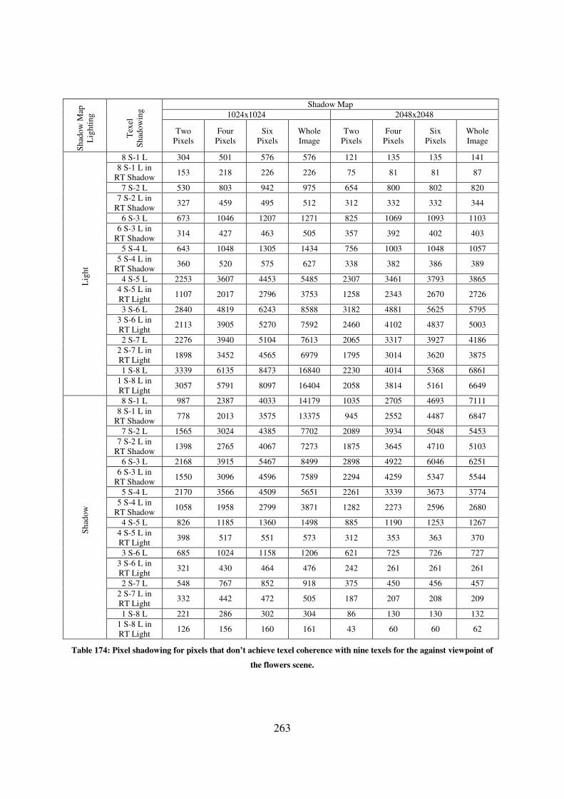
263
Sh
ado
w M
ap
Lig
hti
ng
Tex
el
Sh
ado
win
g Shadow Map
1024x1024 2048x2048
Two
Pixels
Four
Pixels
Six
Pixels
Whole
Image
Two
Pixels
Four
Pixels
Six
Pixels
Whole
Image
Lig
ht
8 S-1 L 304 501 576 576 121 135 135 141
8 S-1 L in
RT Shadow 153 218 226 226 75 81 81 87
7 S-2 L 530 803 942 975 654 800 802 820
7 S-2 L in
RT Shadow 327 459 495 512 312 332 332 344
6 S-3 L 673 1046 1207 1271 825 1069 1093 1103
6 S-3 L in
RT Shadow 314 427 463 505 357 392 402 403
5 S-4 L 643 1048 1305 1434 756 1003 1048 1057
5 S-4 L in
RT Shadow 360 520 575 627 338 382 386 389
4 S-5 L 2253 3607 4453 5485 2307 3461 3793 3865
4 S-5 L in
RT Light 1107 2017 2796 3753 1258 2343 2670 2726
3 S-6 L 2840 4819 6243 8588 3182 4881 5625 5795
3 S-6 L in
RT Light 2113 3905 5270 7592 2460 4102 4837 5003
2 S-7 L 2276 3940 5104 7613 2065 3317 3927 4186
2 S-7 L in
RT Light 1898 3452 4565 6979 1795 3014 3620 3875
1 S-8 L 3339 6135 8473 16840 2230 4014 5368 6861
1 S-8 L in
RT Light 3057 5791 8097 16404 2058 3814 5161 6649
Sh
ado
w
8 S-1 L 987 2387 4033 14179 1035 2705 4693 7111
8 S-1 L in
RT Shadow 778 2013 3575 13375 945 2552 4487 6847
7 S-2 L 1565 3024 4385 7702 2089 3934 5048 5453
7 S-2 L in
RT Shadow 1398 2765 4067 7273 1875 3645 4710 5103
6 S-3 L 2168 3915 5467 8499 2898 4922 6046 6251
6 S-3 L in
RT Shadow 1550 3096 4596 7589 2294 4259 5347 5544
5 S-4 L 2170 3566 4509 5651 2261 3339 3673 3774
5 S-4 L in
RT Shadow 1058 1958 2799 3871 1282 2273 2596 2680
4 S-5 L 826 1185 1360 1498 885 1190 1253 1267
4 S-5 L in
RT Light 398 517 551 573 312 353 363 370
3 S-6 L 685 1024 1158 1206 621 725 726 727
3 S-6 L in
RT Light 321 430 464 476 242 261 261 261
2 S-7 L 548 767 852 918 375 450 456 457
2 S-7 L in
RT Light 332 442 472 505 187 207 208 209
1 S-8 L 221 286 302 304 86 130 130 132
1 S-8 L in
RT Light 126 156 160 161 43 60 60 62
Table 174: Pixel shadowing for pixels that don’t achieve texel coherence with nine texels for the against viewpoint of
the flowers scene.
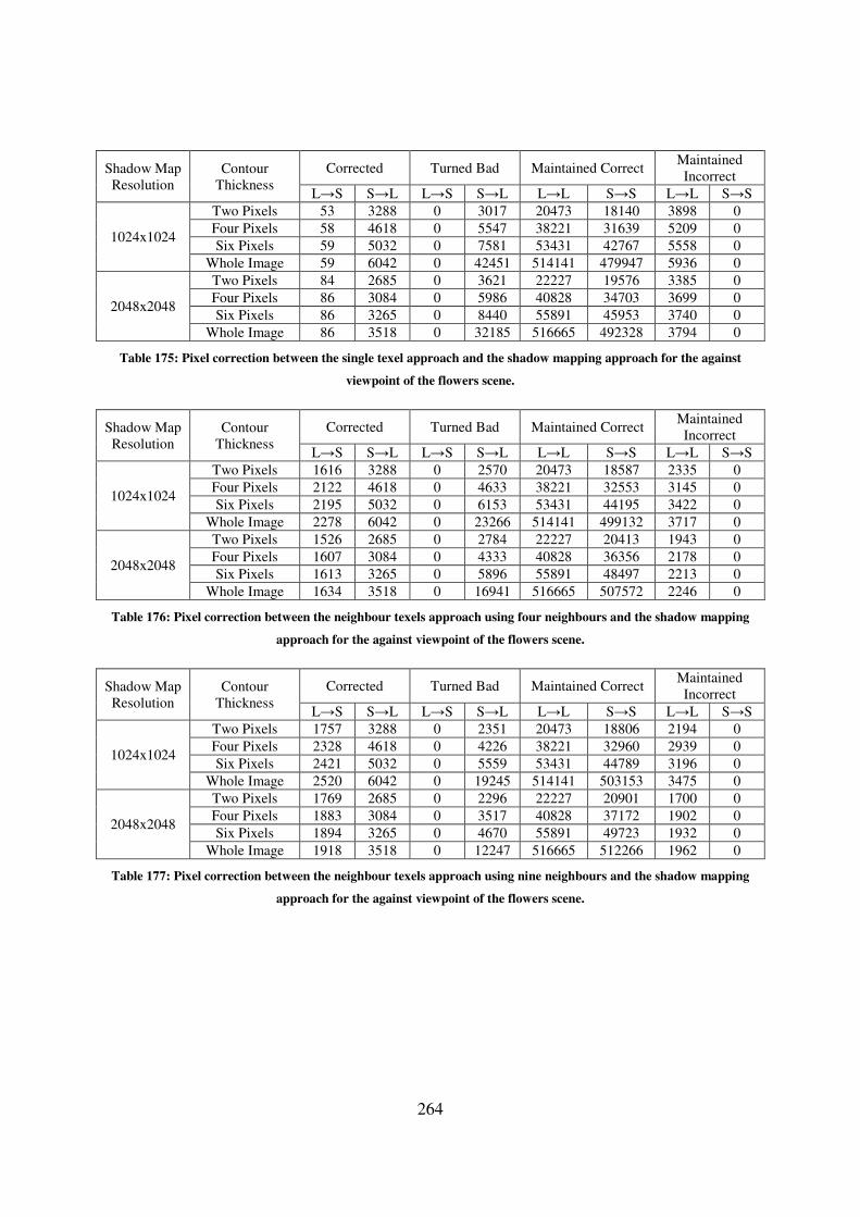
264
Shadow Map
Resolution
Contour
Thickness
Corrected Turned Bad Maintained Correct Maintained
Incorrect
L→S S→L L→S S→L L→L S→S L→L S→S
1024x1024
Two Pixels 53 3288 0 3017 20473 18140 3898 0
Four Pixels 58 4618 0 5547 38221 31639 5209 0
Six Pixels 59 5032 0 7581 53431 42767 5558 0
Whole Image 59 6042 0 42451 514141 479947 5936 0
2048x2048
Two Pixels 84 2685 0 3621 22227 19576 3385 0
Four Pixels 86 3084 0 5986 40828 34703 3699 0
Six Pixels 86 3265 0 8440 55891 45953 3740 0
Whole Image 86 3518 0 32185 516665 492328 3794 0
Table 175: Pixel correction between the single texel approach and the shadow mapping approach for the against
viewpoint of the flowers scene.
Shadow Map
Resolution
Contour
Thickness
Corrected Turned Bad Maintained Correct Maintained
Incorrect
L→S S→L L→S S→L L→L S→S L→L S→S
1024x1024
Two Pixels 1616 3288 0 2570 20473 18587 2335 0
Four Pixels 2122 4618 0 4633 38221 32553 3145 0
Six Pixels 2195 5032 0 6153 53431 44195 3422 0
Whole Image 2278 6042 0 23266 514141 499132 3717 0
2048x2048
Two Pixels 1526 2685 0 2784 22227 20413 1943 0
Four Pixels 1607 3084 0 4333 40828 36356 2178 0
Six Pixels 1613 3265 0 5896 55891 48497 2213 0
Whole Image 1634 3518 0 16941 516665 507572 2246 0
Table 176: Pixel correction between the neighbour texels approach using four neighbours and the shadow mapping
approach for the against viewpoint of the flowers scene.
Shadow Map
Resolution
Contour
Thickness
Corrected Turned Bad Maintained Correct Maintained
Incorrect
L→S S→L L→S S→L L→L S→S L→L S→S
1024x1024
Two Pixels 1757 3288 0 2351 20473 18806 2194 0
Four Pixels 2328 4618 0 4226 38221 32960 2939 0
Six Pixels 2421 5032 0 5559 53431 44789 3196 0
Whole Image 2520 6042 0 19245 514141 503153 3475 0
2048x2048
Two Pixels 1769 2685 0 2296 22227 20901 1700 0
Four Pixels 1883 3084 0 3517 40828 37172 1902 0
Six Pixels 1894 3265 0 4670 55891 49723 1932 0
Whole Image 1918 3518 0 12247 516665 512266 1962 0
Table 177: Pixel correction between the neighbour texels approach using nine neighbours and the shadow mapping
approach for the against viewpoint of the flowers scene.

265
Sh
ado
w M
ap
Res
olu
tio
n
Nu
mb
er o
f
Nei
gh
bo
urs
Tri
ang
le
Av
erag
e
Two Pixels Four Pixels Six Pixels Whole Image
10
24x
102
4
3 Used 2.1533 2.1021 2.0545 0.9310
Available 2.5577 2.4988 2.4580 1.6046
8 Used 3.9267 3.8082 3.7200 1.4111
Available 4.6192 4.4847 4.3664 2.3970
20
48x
204
8
3 Used 2.0065 1.9038 1.8255 0.8386
Available 2.3639 2.3097 2.2575 1.4568
8 Used 3.5757 3.3819 3.2368 1.1931
Available 4.1947 3.9851 3.8410 2.0553
Table 178: Average of triangle intersections when using the neighbour texels approach for the against viewpoint of
the flowers scene.
Shadow Map
Resolution
Contour
Thickness
Corrected Turned Bad Maintained Correct Maintained
Incorrect
L→S S→L L→S S→L L→L S→S L→L S→S
1024x1024
Two Pixels 108 3288 0 2310 20473 18847 3843 0
Four Pixels 130 4618 0 4247 38221 32939 5137 0
Six Pixels 135 5032 0 5613 53431 44735 5482 0
Whole Image 135 6042 0 26409 514141 495989 5860 0
2048x2048
Two Pixels 170 2685 0 2477 22227 20720 3299 0
Four Pixels 181 3084 0 3731 40828 36958 3604 0
Six Pixels 181 3265 0 5483 55891 48910 3645 0
Whole Image 181 3518 0 18686 516665 505827 3699 0
Table 179: Pixel correction between the adjacent geometry approach with one level of adjacency and the shadow
mapping approach for the against viewpoint of the flowers scene.
Shadow Map
Resolution
Contour
Thickness
Corrected Turned Bad Maintained Correct Maintained
Incorrect
L→S S→L L→S S→L L→L S→S L→L S→S
1024x1024
Two Pixels 198 3288 0 1761 20473 19396 3753 0
Four Pixels 247 4618 0 3123 38221 34063 5020 0
Six Pixels 256 5032 0 3954 53431 46394 5361 0
Whole Image 256 6042 0 19836 514141 502562 5739 0
2048x2048
Two Pixels 240 2685 0 1352 22227 21845 3229 0
Four Pixels 266 3084 0 1942 40828 38747 3519 0
Six Pixels 266 3265 0 2942 55891 51451 3560 0
Whole Image 266 3518 0 10729 516665 513784 3614 0
Table 180: Pixel correction between the adjacent geometry approach with two level of adjacency and the shadow
mapping approach for the against viewpoint of the flowers scene.
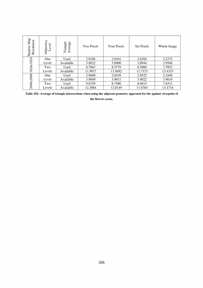
266
Sh
ado
w M
ap
Res
olu
tio
n
Ad
jace
ncy
Lev
el
Tri
ang
le
Av
erag
e
Two Pixels Four Pixels Six Pixels Whole Image
10
24x
102
4
One
Level
Used 2.8186 2.8161 2.8204 2.2372
Available 3.8822 3.8900 3.8944 3.9568
Two
Levels
Used 8.7063 8.5779 8.5006 7.5952
Available 11.9917 11.8492 11.7373 13.4333
20
48x
204
8
One
Level
Used 2.8608 2.8438 2.8525 2.2440
Available 3.9049 3.9011 3.9022 3.9619
Two
Levels
Used 9.0159 8.7586 8.6815 7.6312
Available 12.3064 12.0149 11.8764 13.4734
Table 181: Average of triangle intersections when using the adjacent geometry approach for the against viewpoint of
the flowers scene.

267
Contour Thickness Two Pixels Four Pixels Six Pixels Whole Image
Lighting L→S S→L L→S S→L L→S S→L L→S S→L
Sh
ado
w M
ap R
eso
luti
on
10
24x
102
4
Corrected by
Both 69 3288 77 4618 78 5032 78 6042
Turned Bad
by Both 0 1468 0 2562 0 3146 0 12504
Corrected by
Neighbour
Texels Only
1688 0 2251 0 2343 0 2442 0
Corrected by
Adjacent
Geometry
Only
129 0 170 0 178 0 178 0
Turned Bad
by
Neighbour
Texels Only
0 883 0 1664 0 2413 0 6471
Turned Bad
by Adjacent
Geometry
Only
0 293 0 561 0 808 0 7332
20
48x
204
8
Corrected by
Both 140 2685 147 3084 147 3265 147 3518
Turned Bad
by Both 0 957 0 1318 0 1902 0 5435
Corrected by
Neighbour
Texels Only
1629 0 1736 0 1747 0 1771 0
Corrected by
Adjacent
Geometry
Only
100 0 119 0 119 0 119 0
Turned Bad
by
Neighbour
Texels Only
0 1339 0 2199 0 2768 0 6812
Turned Bad
by Adjacent
Geometry
Only
0 395 0 624 0 1040 0 5294
Table 182: Pixel correction by the neighbour texels (9 texels) and the adjacent geometry (2 levels) approaches
separated by lighting change for the against viewpoint of the flowers scene.
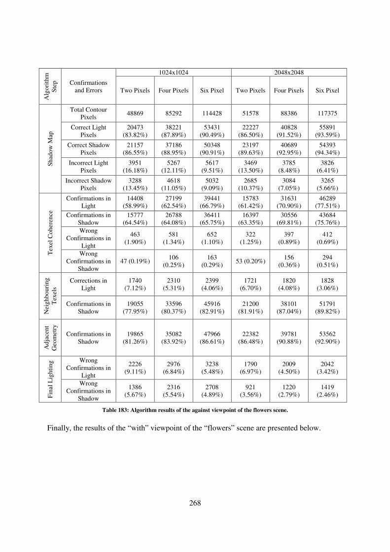
268
Alg
ori
thm
Ste
p
Confirmations
and Errors
1024x1024 2048x2048
Two Pixels Four Pixels Six Pixel Two Pixels Four Pixels Six Pixel
Sh
ado
w M
ap
Total Contour
Pixels 48869 85292 114428 51578 88386 117375
Correct Light
Pixels
20473
(83.82%)
38221
(87.89%)
53431
(90.49%)
22227
(86.50%)
40828
(91.52%)
55891
(93.59%)
Correct Shadow
Pixels
21157
(86.55%)
37186
(88.95%)
50348
(90.91%)
23197
(89.63%)
40689
(92.95%)
54393
(94.34%)
Incorrect Light
Pixels
3951
(16.18%)
5267
(12.11%)
5617
(9.51%)
3469
(13.50%)
3785
(8.48%)
3826
(6.41%)
Incorrect Shadow
Pixels
3288
(13.45%)
4618
(11.05%)
5032
(9.09%)
2685
(10.37%)
3084
(7.05%)
3265
(5.66%)
Tex
el C
oh
eren
ce
Confirmations in
Light
14408
(58.99%)
27199
(62.54%)
39441
(66.79%)
15783
(61.42%)
31631
(70.90%)
46289
(77.51%)
Confirmations in
Shadow
15777
(64.54%)
26788
(64.08%)
36411
(65.75%)
16397
(63.35%)
30556
(69.81%)
43684
(75.76%)
Wrong
Confirmations in
Light
463
(1.90%)
581
(1.34%)
652
(1.10%)
322
(1.25%)
397
(0.89%)
412
(0.69%)
Wrong
Confirmations in
Shadow
47 (0.19%) 106
(0.25%)
163
(0.29%) 53 (0.20%)
156
(0.36%)
294
(0.51%)
Nei
gh
bo
uri
ng
Tex
els
Corrections in
Light
1740
(7.12%)
2310
(5.31%)
2399
(4.06%)
1721
(6.70%)
1820
(4.08%)
1828
(3.06%)
Confirmations in
Shadow
19055
(77.95%)
33596
(80.37%)
45916
(82.91%)
21200
(81.91%)
38101
(87.04%)
51791
(89.82%)
Ad
jace
nt
Geo
met
ry
Confirmations in
Shadow
19865
(81.26%)
35082
(83.92%)
47966
(86.61%)
22382
(86.48%)
39781
(90.88%)
53562
(92.90%)
Fin
al L
igh
tin
g Wrong
Confirmations in
Light
2226
(9.11%)
2976
(6.84%)
3238
(5.48%)
1790
(6.97%)
2009
(4.50%)
2042
(3.42%)
Wrong
Confirmations in
Shadow
1386
(5.67%)
2316
(5.54%)
2708
(4.89%)
921
(3.56%)
1220
(2.79%)
1419
(2.46%)
Table 183: Algorithm results of the against viewpoint of the flowers scene.
Finally, the results of the “with” viewpoint of the “flowers” scene are presented below.
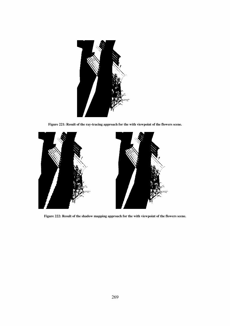
Figure 221: Result of the ray
Figure 222: Result of the shadow mapping approach for the
269
of the ray-tracing approach for the with viewpoint of the flowers scene.
: Result of the shadow mapping approach for the with viewpoint of the flowers
tracing approach for the with viewpoint of the flowers scene.
flowers scene.
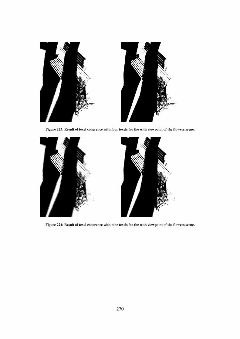
Figure 223: Result of texel coherence with four texels for
Figure 224: Result of texel coherence with nine texels for
270
: Result of texel coherence with four texels for the with viewpoint of the flowers scene
: Result of texel coherence with nine texels for the with viewpoint of the flowers scene
the with viewpoint of the flowers scene.
the with viewpoint of the flowers scene.
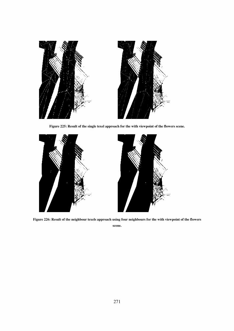
271
Figure 225: Result of the single texel approach for the with viewpoint of the flowers scene.
Figure 226: Result of the neighbour texels approach using four neighbours for the with viewpoint of the flowers
scene.
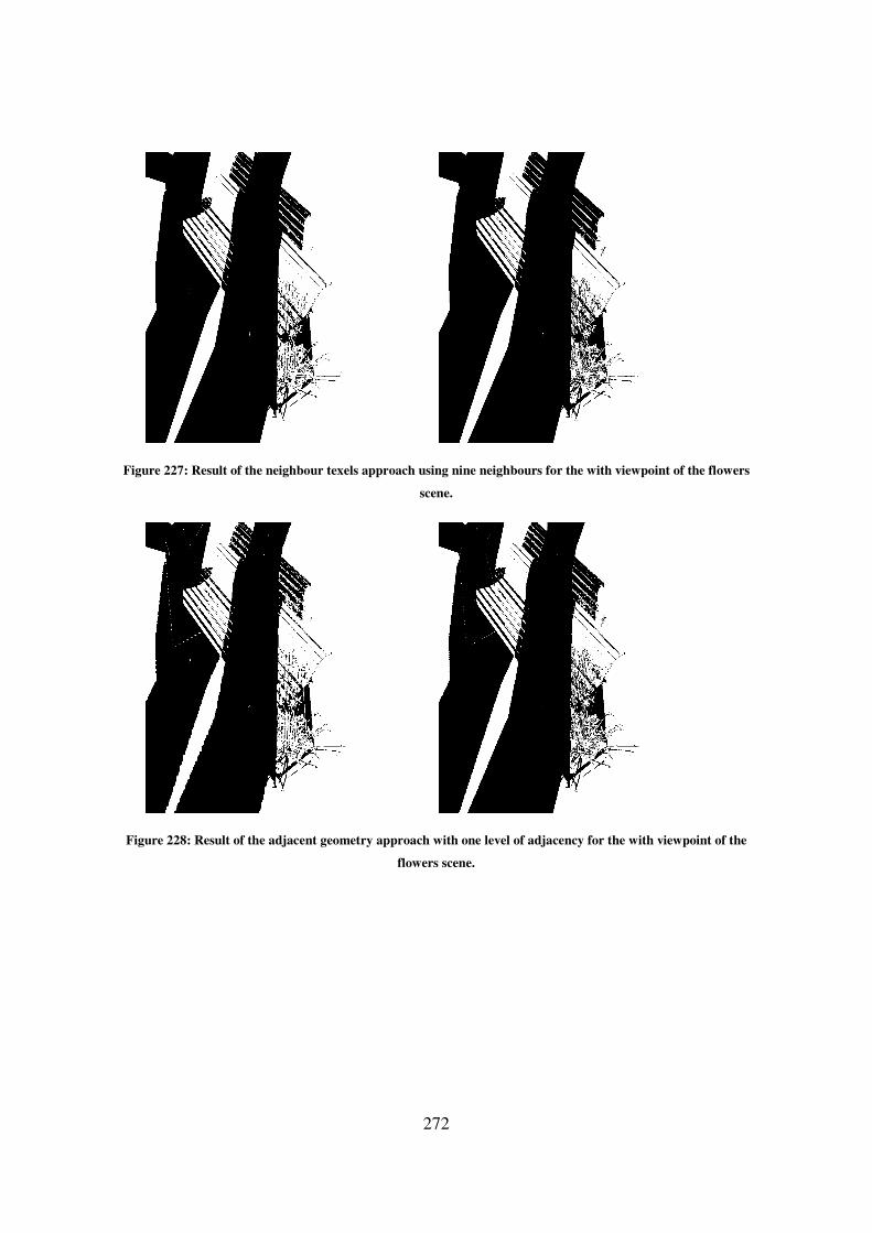
272
Figure 227: Result of the neighbour texels approach using nine neighbours for the with viewpoint of the flowers
scene.
Figure 228: Result of the adjacent geometry approach with one level of adjacency for the with viewpoint of the
flowers scene.
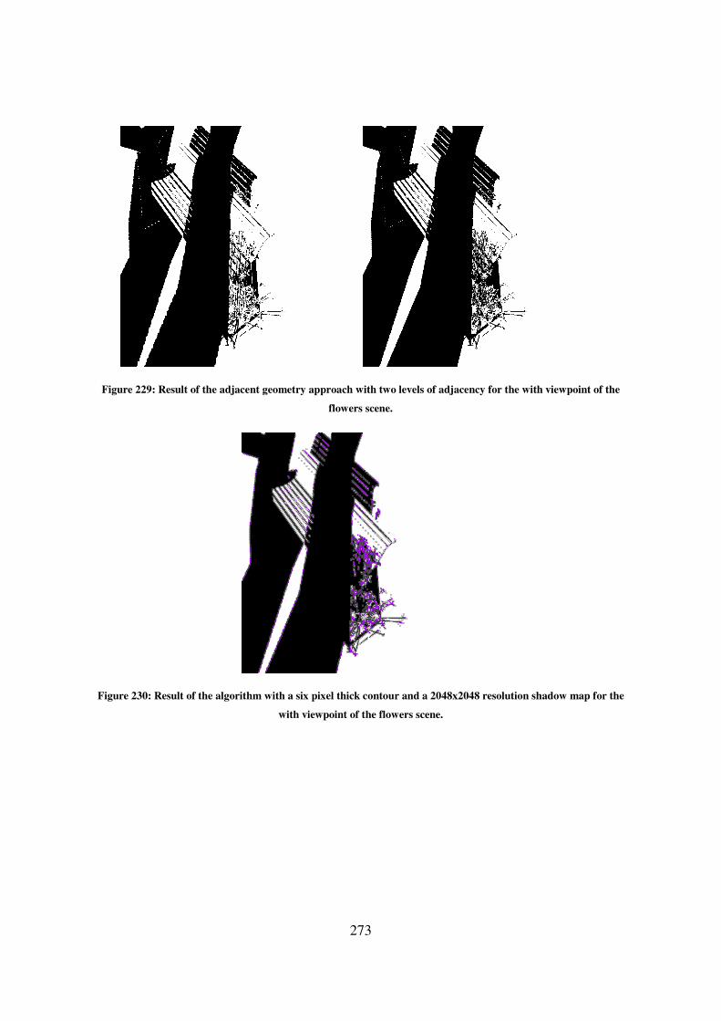
Figure 229: Result of the adjacent geometry
Figure 230: Result of the algorithm w
273
adjacent geometry approach with two levels of adjacency for the with viewpoint of the
flowers scene.
: Result of the algorithm with a six pixel thick contour and a 2048x2048 resolution shadow map for the
with viewpoint of the flowers scene.
the with viewpoint of the
ith a six pixel thick contour and a 2048x2048 resolution shadow map for the
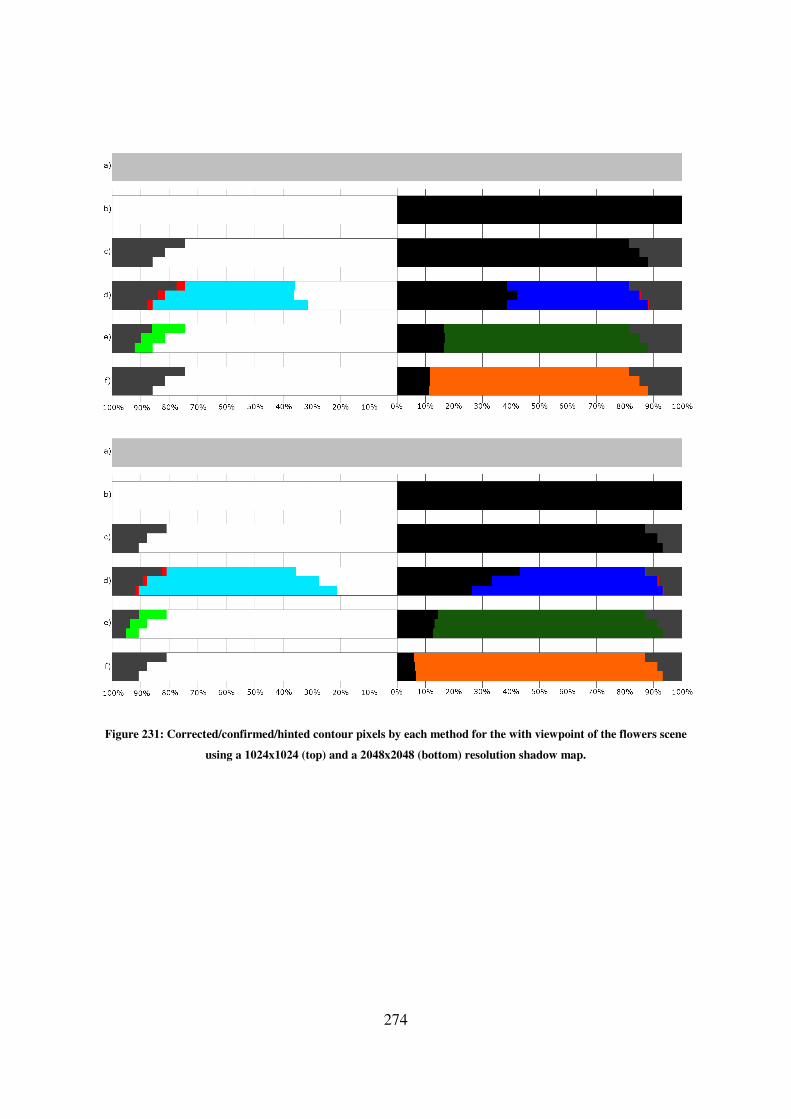
274
Figure 231: Corrected/confirmed/hinted contour pixels by each method for the with viewpoint of the flowers scene
using a 1024x1024 (top) and a 2048x2048 (bottom) resolution shadow map.
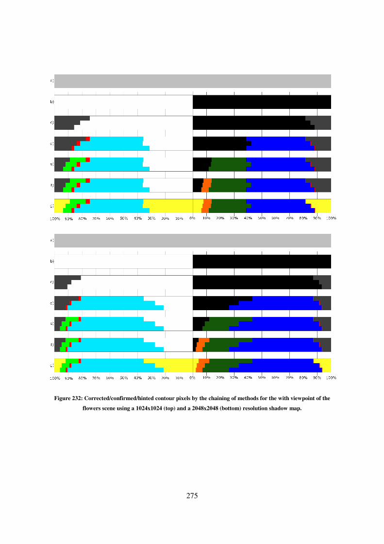
275
Figure 232: Corrected/confirmed/hinted contour pixels by the chaining of methods for the with viewpoint of the
flowers scene using a 1024x1024 (top) and a 2048x2048 (bottom) resolution shadow map.

276
Shadow Map
Resolution Approach
Contour Thickness
Two Pixels Four Pixels Six Pixels Whole Image
1024x1024
Pixels in
Contour 47045 82557 111069 1048576
Shadow Map 10457 (22.23%) 13806 (16.72%) 14567 (13.12%) 15230 (1.45%)
Single Texel 11660 (24.78%) 18038 (21.85%) 21958 (19.77%) 43091 (4.11%)
Neighbour
Texels (4
Neighbours)
7994 (16.99%) 12578 (15.24%) 15247 (13.73%) 22742 (2.17%)
Neighbour
Texels (9
Neighbours)
7136 (15.17%) 11083 (13.42%) 13419 (12.08%) 19799 (1.89%)
Adjacent
Geometry (One
Level)
9959 (21.17%) 14750 (17.87%) 17406 (15.67%) 26192 (2.50%)
Adjacent
Geometry
(Two Level)
8585 (18.25%) 12121 (14.68%) 13820 (12.44%) 20171 (1.92%)
2048x2048
Pixels in
Contour 50263 85450 113229 1048576
Shadow Map 8050 (16.02%) 8919 (10.44%) 9099 (8.04%) 9245 (0.88%)
Single Texel 10740 (21.37%) 15196 (17.78%) 18211 (16.08%) 30531 (2.91%)
Neighbour
Texels (4
Neighbours)
7054 (14.03%) 9821 (11.49%) 11739 (10.37%) 16311 (1.56%)
Neighbour
Texels (9
Neighbours)
6012 (11.96%) 8284 (9.69%) 9845 (8.69%) 13388 (1.28%)
Adjacent
Geometry (One
Level)
8176 (16.27%) 10691 (12.51%) 12527 (11.06%) 17358 (1.66%)
Adjacent
Geometry(Two
Level)
6169 (12.27%) 7498 (8.77%) 8501 (7.51%) 11249 (1.07%)
Table 184: Difference between the approaches that use ray-tracing and the actual ray-tracer for the with viewpoint of
the flowers scene.
Shadow Map Resolution Contour Thickness
Two Pixels Four Pixels Six Pixels
1024x1024 10457 of 15230 (68.66%) 13806 of 15230 (90.65%) 14567 of 15230 (95.65%)
2048x2048 8050 of 9245 (87.07%) 8919 of 9245 (96.47%) 9099 of 9245 (98.42%)
Table 185: Wrongly defined pixels in the shadow mapping result which are inside the contour in the with viewpoint
of the flowers scene.
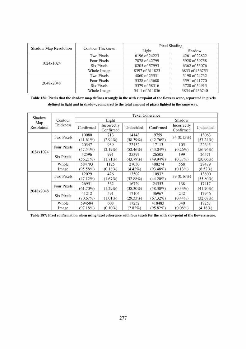
277
Shadow Map Resolution Contour Thickness Pixel Shading
Light Shadow
1024x1024
Two Pixels 6196 of 24223 4261 of 22822
Four Pixels 7878 of 42799 5928 of 39758
Six Pixels 8205 of 57993 6362 of 53076
Whole Image 8397 of 611823 6833 of 436753
2048x2048
Two Pixels 4860 of 25531 3190 of 24732
Four Pixels 5328 of 43680 3591 of 41770
Six Pixels 5379 of 58316 3720 of 54913
Whole Image 5411 of 611836 3834 of 436740
Table 186: Pixels that the shadow map defines wrongly in the with viewpoint of the flowers scene, separated in pixels
defined in light and in shadow, compared to the total amount of pixels lighted in the same way.
Shadow
Map
Resolution
Contour
Thickness
Texel Coherence
Light Shadow
Confirmed Incorrectly
Confirmed Undecided Confirmed
Incorrectly
Confirmed Undecided
1024x1024
Two Pixels 10080
(41.61%)
713
(2.94%)
14143
(58.39%)
9759
(42.76%) 34 (0.15%)
13063
(57.24%)
Four Pixels 20347
(47.54%)
939
(2.19%)
22452
(52.46%)
17113
(43.04%)
105
(0.26%)
22645
(56.96%)
Six Pixels 32596
(56.21%)
991
(1.71%)
25397
(43.79%)
26505
(49.94%)
199
(0.37%)
26571
(50.06%)
Whole
Image
584793
(95.58%)
1125
(0.18%)
27030
(4.42%)
408274
(93.48%)
568
(0.13%)
28479
(6.52%)
2048x2048
Two Pixels 12029
(47.12%)
426
(1.67%)
13502
(52.88%)
10932
(44.20%) 39 (0.16%)
13800
(55.80%)
Four Pixels 26951
(61.70%)
562
(1.29%)
16729
(38.30%)
24353
(58.30%)
138
(0.33%)
17417
(41.70%)
Six Pixels 41212
(70.67%)
591
(1.01%)
17104
(29.33%)
36967
(67.32%)
242
(0.44%)
17946
(32.68%)
Whole
Image
594584
(97.18%)
608
(0.10%)
17252
(2.82%)
418483
(95.82%)
340
(0.08%)
18257
(4.18%)
Table 187: Pixel confirmation when using texel coherence with four texels for the with viewpoint of the flowers scene.
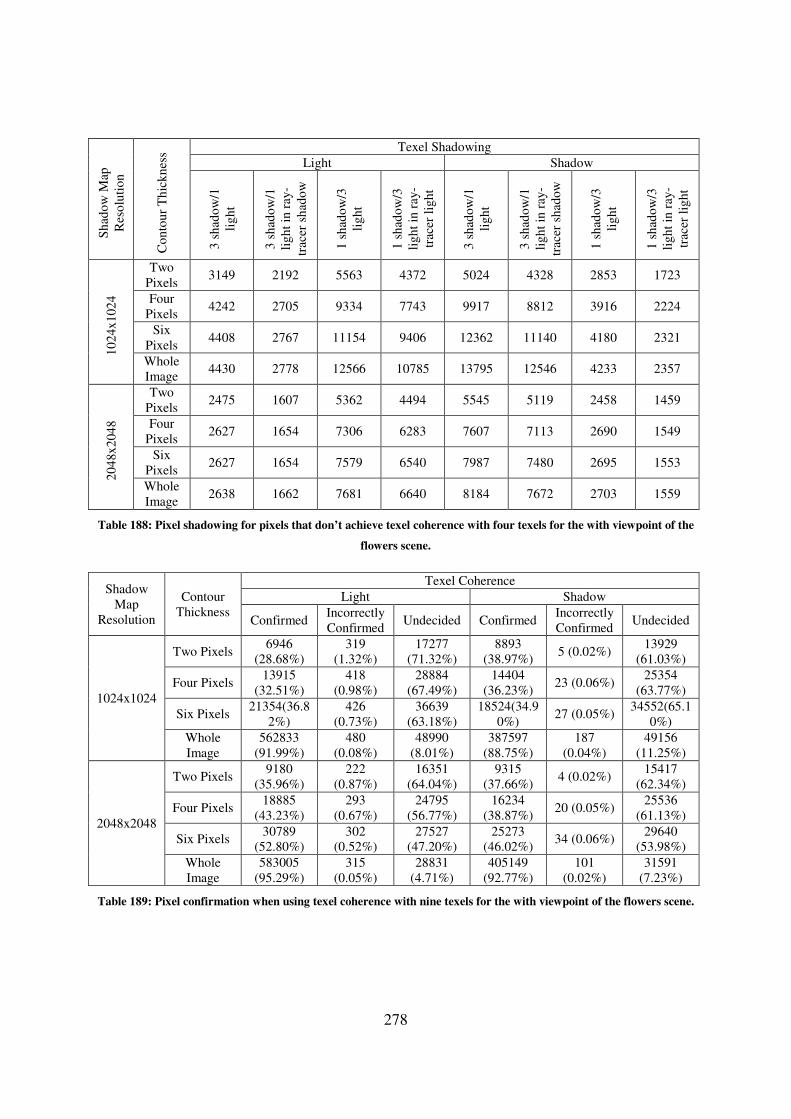
278
Sh
ado
w M
ap
Res
olu
tio
n
Co
nto
ur
Th
ick
nes
s Texel Shadowing
Light Shadow
3 s
had
ow
/1
lig
ht
3 s
had
ow
/1
lig
ht
in r
ay-
trac
er s
had
ow
1 s
had
ow
/3
lig
ht
1 s
had
ow
/3
lig
ht
in r
ay-
trac
er l
igh
t
3 s
had
ow
/1
lig
ht
3 s
had
ow
/1
lig
ht
in r
ay-
trac
er s
had
ow
1 s
had
ow
/3
lig
ht
1 s
had
ow
/3
lig
ht
in r
ay-
trac
er l
igh
t
10
24x
102
4
Two
Pixels 3149 2192 5563 4372 5024 4328 2853 1723
Four
Pixels 4242 2705 9334 7743 9917 8812 3916 2224
Six
Pixels 4408 2767 11154 9406 12362 11140 4180 2321
Whole
Image 4430 2778 12566 10785 13795 12546 4233 2357
20
48x
204
8
Two
Pixels 2475 1607 5362 4494 5545 5119 2458 1459
Four
Pixels 2627 1654 7306 6283 7607 7113 2690 1549
Six
Pixels 2627 1654 7579 6540 7987 7480 2695 1553
Whole
Image 2638 1662 7681 6640 8184 7672 2703 1559
Table 188: Pixel shadowing for pixels that don’t achieve texel coherence with four texels for the with viewpoint of the
flowers scene.
Shadow
Map
Resolution
Contour
Thickness
Texel Coherence
Light Shadow
Confirmed Incorrectly
Confirmed Undecided Confirmed
Incorrectly
Confirmed Undecided
1024x1024
Two Pixels 6946
(28.68%)
319
(1.32%)
17277
(71.32%)
8893
(38.97%) 5 (0.02%)
13929
(61.03%)
Four Pixels 13915
(32.51%)
418
(0.98%)
28884
(67.49%)
14404
(36.23%) 23 (0.06%)
25354
(63.77%)
Six Pixels 21354(36.8
2%)
426
(0.73%)
36639
(63.18%)
18524(34.9
0%) 27 (0.05%)
34552(65.1
0%)
Whole
Image
562833
(91.99%)
480
(0.08%)
48990
(8.01%)
387597
(88.75%)
187
(0.04%)
49156
(11.25%)
2048x2048
Two Pixels 9180
(35.96%)
222
(0.87%)
16351
(64.04%)
9315
(37.66%) 4 (0.02%)
15417
(62.34%)
Four Pixels 18885
(43.23%)
293
(0.67%)
24795
(56.77%)
16234
(38.87%) 20 (0.05%)
25536
(61.13%)
Six Pixels 30789
(52.80%)
302
(0.52%)
27527
(47.20%)
25273
(46.02%) 34 (0.06%)
29640
(53.98%)
Whole
Image
583005
(95.29%)
315
(0.05%)
28831
(4.71%)
405149
(92.77%)
101
(0.02%)
31591
(7.23%)
Table 189: Pixel confirmation when using texel coherence with nine texels for the with viewpoint of the flowers scene.
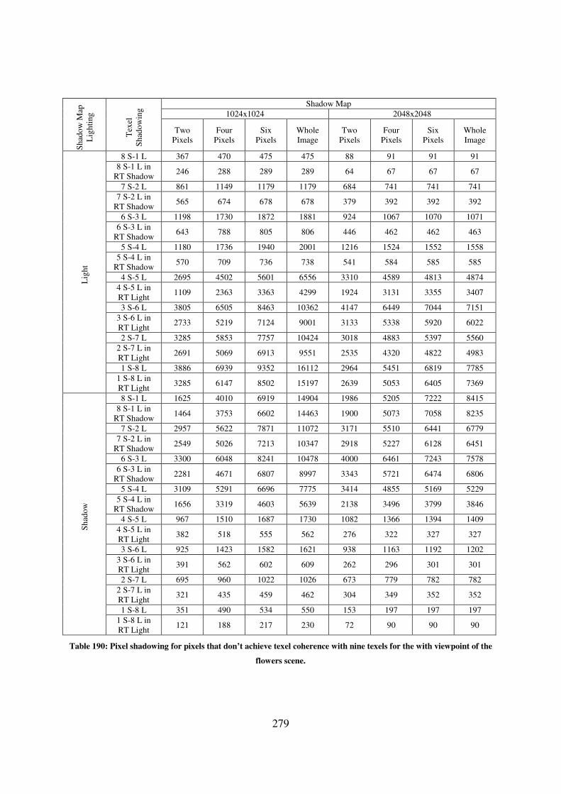
279
Sh
ado
w M
ap
Lig
hti
ng
Tex
el
Sh
ado
win
g Shadow Map
1024x1024 2048x2048
Two
Pixels
Four
Pixels
Six
Pixels
Whole
Image
Two
Pixels
Four
Pixels
Six
Pixels
Whole
Image
Lig
ht
8 S-1 L 367 470 475 475 88 91 91 91
8 S-1 L in
RT Shadow 246 288 289 289 64 67 67 67
7 S-2 L 861 1149 1179 1179 684 741 741 741
7 S-2 L in
RT Shadow 565 674 678 678 379 392 392 392
6 S-3 L 1198 1730 1872 1881 924 1067 1070 1071
6 S-3 L in
RT Shadow 643 788 805 806 446 462 462 463
5 S-4 L 1180 1736 1940 2001 1216 1524 1552 1558
5 S-4 L in
RT Shadow 570 709 736 738 541 584 585 585
4 S-5 L 2695 4502 5601 6556 3310 4589 4813 4874
4 S-5 L in
RT Light 1109 2363 3363 4299 1924 3131 3355 3407
3 S-6 L 3805 6505 8463 10362 4147 6449 7044 7151
3 S-6 L in
RT Light 2733 5219 7124 9001 3133 5338 5920 6022
2 S-7 L 3285 5853 7757 10424 3018 4883 5397 5560
2 S-7 L in
RT Light 2691 5069 6913 9551 2535 4320 4822 4983
1 S-8 L 3886 6939 9352 16112 2964 5451 6819 7785
1 S-8 L in
RT Light 3285 6147 8502 15197 2639 5053 6405 7369
Sh
ado
w
8 S-1 L 1625 4010 6919 14904 1986 5205 7222 8415
8 S-1 L in
RT Shadow 1464 3753 6602 14463 1900 5073 7058 8235
7 S-2 L 2957 5622 7871 11072 3171 5510 6441 6779
7 S-2 L in
RT Shadow 2549 5026 7213 10347 2918 5227 6128 6451
6 S-3 L 3300 6048 8241 10478 4000 6461 7243 7578
6 S-3 L in
RT Shadow 2281 4671 6807 8997 3343 5721 6474 6806
5 S-4 L 3109 5291 6696 7775 3414 4855 5169 5229
5 S-4 L in
RT Shadow 1656 3319 4603 5639 2138 3496 3799 3846
4 S-5 L 967 1510 1687 1730 1082 1366 1394 1409
4 S-5 L in
RT Light 382 518 555 562 276 322 327 327
3 S-6 L 925 1423 1582 1621 938 1163 1192 1202
3 S-6 L in
RT Light 391 562 602 609 262 296 301 301
2 S-7 L 695 960 1022 1026 673 779 782 782
2 S-7 L in
RT Light 321 435 459 462 304 349 352 352
1 S-8 L 351 490 534 550 153 197 197 197
1 S-8 L in
RT Light 121 188 217 230 72 90 90 90
Table 190: Pixel shadowing for pixels that don’t achieve texel coherence with nine texels for the with viewpoint of the
flowers scene.
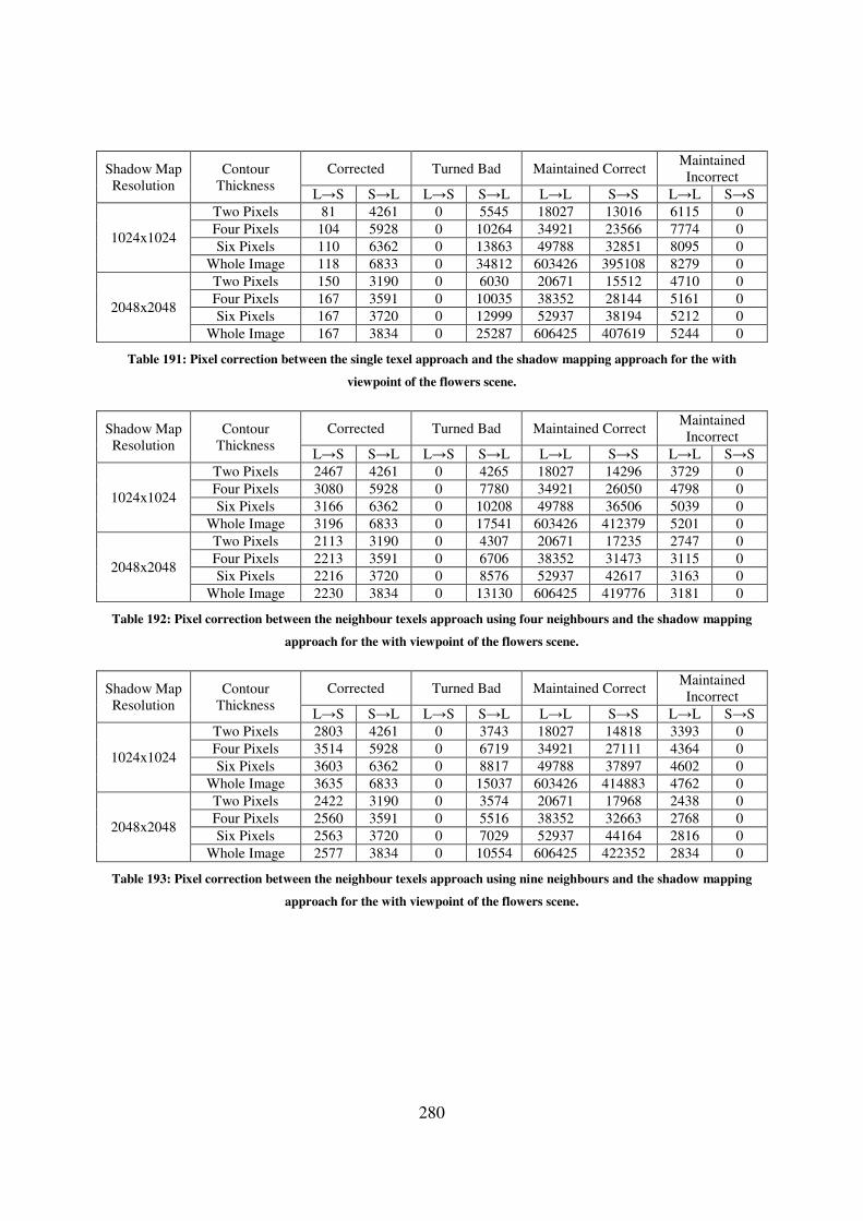
280
Shadow Map
Resolution
Contour
Thickness
Corrected Turned Bad Maintained Correct Maintained
Incorrect
L→S S→L L→S S→L L→L S→S L→L S→S
1024x1024
Two Pixels 81 4261 0 5545 18027 13016 6115 0
Four Pixels 104 5928 0 10264 34921 23566 7774 0
Six Pixels 110 6362 0 13863 49788 32851 8095 0
Whole Image 118 6833 0 34812 603426 395108 8279 0
2048x2048
Two Pixels 150 3190 0 6030 20671 15512 4710 0
Four Pixels 167 3591 0 10035 38352 28144 5161 0
Six Pixels 167 3720 0 12999 52937 38194 5212 0
Whole Image 167 3834 0 25287 606425 407619 5244 0
Table 191: Pixel correction between the single texel approach and the shadow mapping approach for the with
viewpoint of the flowers scene.
Shadow Map
Resolution
Contour
Thickness
Corrected Turned Bad Maintained Correct Maintained
Incorrect
L→S S→L L→S S→L L→L S→S L→L S→S
1024x1024
Two Pixels 2467 4261 0 4265 18027 14296 3729 0
Four Pixels 3080 5928 0 7780 34921 26050 4798 0
Six Pixels 3166 6362 0 10208 49788 36506 5039 0
Whole Image 3196 6833 0 17541 603426 412379 5201 0
2048x2048
Two Pixels 2113 3190 0 4307 20671 17235 2747 0
Four Pixels 2213 3591 0 6706 38352 31473 3115 0
Six Pixels 2216 3720 0 8576 52937 42617 3163 0
Whole Image 2230 3834 0 13130 606425 419776 3181 0
Table 192: Pixel correction between the neighbour texels approach using four neighbours and the shadow mapping
approach for the with viewpoint of the flowers scene.
Shadow Map
Resolution
Contour
Thickness
Corrected Turned Bad Maintained Correct Maintained
Incorrect
L→S S→L L→S S→L L→L S→S L→L S→S
1024x1024
Two Pixels 2803 4261 0 3743 18027 14818 3393 0
Four Pixels 3514 5928 0 6719 34921 27111 4364 0
Six Pixels 3603 6362 0 8817 49788 37897 4602 0
Whole Image 3635 6833 0 15037 603426 414883 4762 0
2048x2048
Two Pixels 2422 3190 0 3574 20671 17968 2438 0
Four Pixels 2560 3591 0 5516 38352 32663 2768 0
Six Pixels 2563 3720 0 7029 52937 44164 2816 0
Whole Image 2577 3834 0 10554 606425 422352 2834 0
Table 193: Pixel correction between the neighbour texels approach using nine neighbours and the shadow mapping
approach for the with viewpoint of the flowers scene.

281
Sh
ado
w M
ap
Res
olu
tio
n
Nu
mb
er o
f
Nei
gh
bo
urs
Tri
ang
le
Av
erag
e
Two Pixels Four Pixels Six Pixels Whole Image
10
24x
102
4
3 Used 2.4112 2.3467 2.2626 0.7686
Available 2.5506 2.4912 2.4558 1.5562
8 Used 4.4772 4.3261 4.1689 1.1469
Available 4.7030 4.5393 4.3816 2.2792
20
48x
204
8
3 Used 2.2667 2.1329 2.0153 0.6925
Available 2.4164 2.3558 2.2805 1.4165
8 Used 4.0599 3.8321 3.6037 0.9629
Available 4.2812 4.0566 3.8968 1.9494
Table 194: Average of triangle intersections when using the neighbour texels approach for the with viewpoint of the
flowers scene.
Shadow Map
Resolution
Contour
Thickness
Corrected Turned Bad Maintained Correct Maintained
Incorrect
L→S S→L L→S S→L L→L S→S L→L S→S
1024x1024
Two Pixels 165 4261 0 3928 18027 14633 6031 0
Four Pixels 228 5928 0 7100 34921 26730 7650 0
Six Pixels 244 6362 0 9445 49788 37269 7961 0
Whole Image 257 6833 0 18052 603426 411868 8140 0
2048x2048
Two Pixels 287 3190 0 3603 20671 17939 4573 0
Four Pixels 341 3591 0 5704 38352 32475 4987 0
Six Pixels 346 3720 0 7494 52937 43699 5033 0
Whole Image 346 3834 0 12293 606425 420613 5065 0
Table 195: Pixel correction between the adjacent geometry approach with one level of adjacency and the shadow
mapping approach for the with viewpoint of the flowers scene.
Shadow Map
Resolution
Contour
Thickness
Corrected Turned Bad Maintained Correct Maintained
Incorrect
L→S S→L L→S S→L L→L S→S L→L S→S
1024x1024
Two Pixels 268 4261 0 2657 18027 15904 5928 0
Four Pixels 398 5928 0 4641 34921 29189 7480 0
Six Pixels 429 6362 0 6044 49788 40670 7776 0
Whole Image 452 6833 0 12226 603426 417694 7945 0
2048x2048
Two Pixels 395 3190 0 1704 20671 19838 4465 0
Four Pixels 494 3591 0 2664 38352 35515 4834 0
Six Pixels 504 3720 0 3626 52937 47567 4875 0
Whole Image 507 3834 0 6345 606425 426561 4904 0
Table 196: Pixel correction between the adjacent geometry approach with two level of adjacency and the shadow
mapping approach for the with viewpoint of the flowers scene.

282
Sh
ado
w M
ap
Res
olu
tio
n
Ad
jace
ncy
Lev
el
Tri
ang
le
Av
erag
e
Two Pixels Four Pixels Six Pixels Whole Image
10
24x
102
4
One
Level
Used 3.0413 3.0660 3.0733 1.8966
Available 3.8668 3.8695 3.8740 3.9621
Two
Levels
Used 9.6289 9.6693 9.6106 6.4508
Available 12.2423 12.2033 12.1147 13.4759
20
48x
204
8
One
Level
Used 3.0904 3.1070 3.1055 1.9001
Available 3.8679 3.8638 3.8649 3.9595
Two
Levels
Used 9.7832 9.6871 9.5584 6.4438
Available 12.2443 12.0465 11.8957 13.4276
Table 197: Average of triangle intersections when using the adjacent geometry approach for the with viewpoint of the
flowers scene.

283
Contour Thickness Two Pixels Four Pixels Six Pixels Whole Image
Lighting L→S S→L L→S S→L L→S S→L L→S S→L
Sh
ado
w M
ap R
eso
luti
on
10
24x
102
4
Corrected by
Both 97 4261 128 5928 135 6362 143 6833
Turned Bad
by Both 0 2205 0 3825 0 4922 0 9037
Corrected by
Neighbour
Texels Only
2706 0 3386 0 3468 0 3492 0
Corrected by
Adjacent
Geometry
Only
171 0 270 0 294 0 309 0
Turned Bad
by
Neighbour
Texels Only
0 1538 0 2894 0 3895 0 6000
Turned Bad
by Adjacent
Geometry
Only
0 452 0 816 0 1122 0 3189
20
48x
204
8
Corrected by
Both 218 3190 250 3591 252 3720 252 3834
Turned Bad
by Both 0 1298 0 1923 0 2610 0 4227
Corrected by
Neighbour
Texels Only
2204 0 2310 0 2311 0 2325 0
Corrected by
Adjacent
Geometry
Only
177 0 244 0 252 0 255 0
Turned Bad
by
Neighbour
Texels Only
0 2276 0 3593 0 4419 0 6327
Turned Bad
by Adjacent
Geometry
Only
0 406 0 741 0 1016 0 2118
Table 198: Pixel correction by the neighbour texels (9 texels) and the adjacent geometry (2 levels) approaches
separated by lighting change for the with viewpoint of the flowers scene.
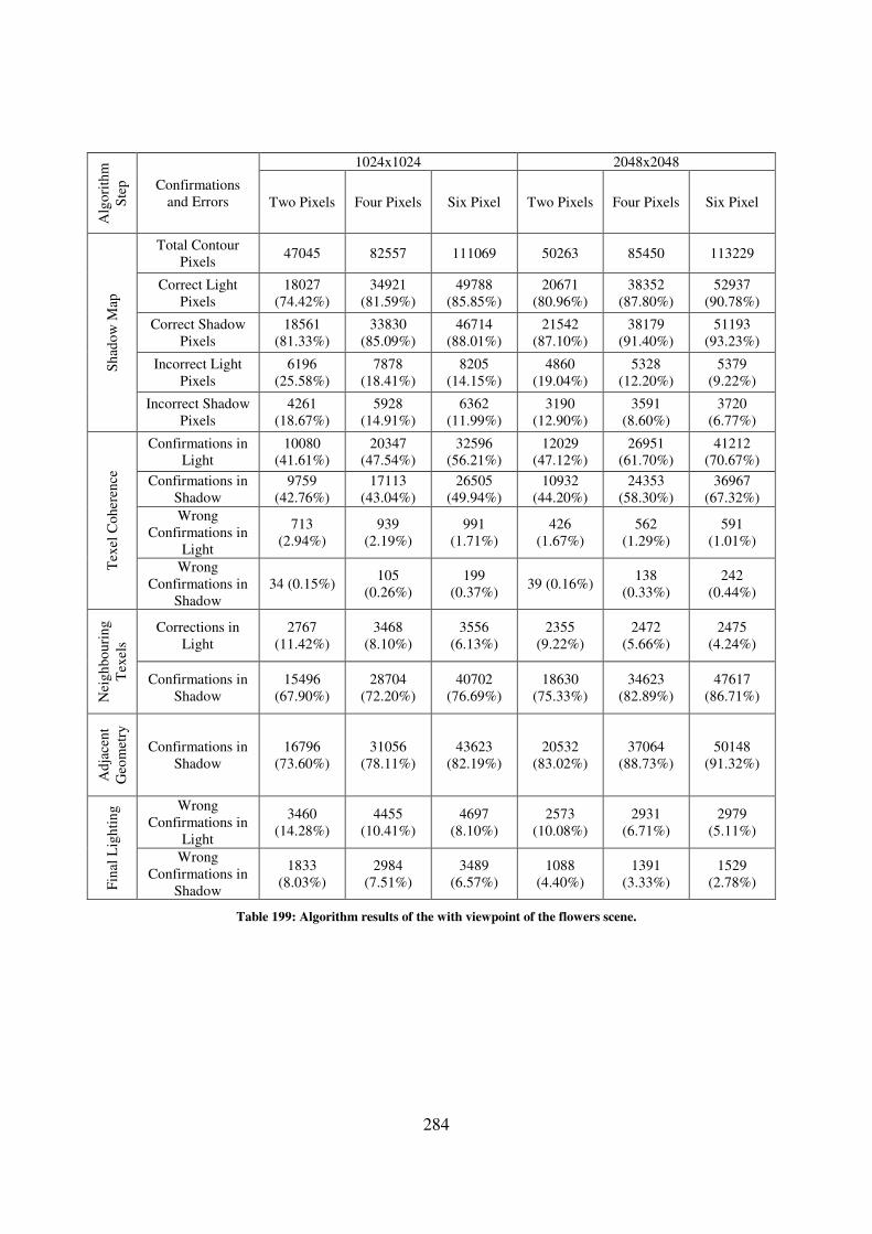
284
Alg
ori
thm
Ste
p
Confirmations
and Errors
1024x1024 2048x2048
Two Pixels Four Pixels Six Pixel Two Pixels Four Pixels Six Pixel
Sh
ado
w M
ap
Total Contour
Pixels 47045 82557 111069 50263 85450 113229
Correct Light
Pixels
18027
(74.42%)
34921
(81.59%)
49788
(85.85%)
20671
(80.96%)
38352
(87.80%)
52937
(90.78%)
Correct Shadow
Pixels
18561
(81.33%)
33830
(85.09%)
46714
(88.01%)
21542
(87.10%)
38179
(91.40%)
51193
(93.23%)
Incorrect Light
Pixels
6196
(25.58%)
7878
(18.41%)
8205
(14.15%)
4860
(19.04%)
5328
(12.20%)
5379
(9.22%)
Incorrect Shadow
Pixels
4261
(18.67%)
5928
(14.91%)
6362
(11.99%)
3190
(12.90%)
3591
(8.60%)
3720
(6.77%)
Tex
el C
oh
eren
ce
Confirmations in
Light
10080
(41.61%)
20347
(47.54%)
32596
(56.21%)
12029
(47.12%)
26951
(61.70%)
41212
(70.67%)
Confirmations in
Shadow
9759
(42.76%)
17113
(43.04%)
26505
(49.94%)
10932
(44.20%)
24353
(58.30%)
36967
(67.32%)
Wrong
Confirmations in
Light
713
(2.94%)
939
(2.19%)
991
(1.71%)
426
(1.67%)
562
(1.29%)
591
(1.01%)
Wrong
Confirmations in
Shadow
34 (0.15%) 105
(0.26%)
199
(0.37%) 39 (0.16%)
138
(0.33%)
242
(0.44%)
Nei
gh
bo
uri
ng
Tex
els
Corrections in
Light
2767
(11.42%)
3468
(8.10%)
3556
(6.13%)
2355
(9.22%)
2472
(5.66%)
2475
(4.24%)
Confirmations in
Shadow
15496
(67.90%)
28704
(72.20%)
40702
(76.69%)
18630
(75.33%)
34623
(82.89%)
47617
(86.71%)
Ad
jace
nt
Geo
met
ry
Confirmations in
Shadow
16796
(73.60%)
31056
(78.11%)
43623
(82.19%)
20532
(83.02%)
37064
(88.73%)
50148
(91.32%)
Fin
al L
igh
tin
g Wrong
Confirmations in
Light
3460
(14.28%)
4455
(10.41%)
4697
(8.10%)
2573
(10.08%)
2931
(6.71%)
2979
(5.11%)
Wrong
Confirmations in
Shadow
1833
(8.03%)
2984
(7.51%)
3489
(6.57%)
1088
(4.40%)
1391
(3.33%)
1529
(2.78%)
Table 199: Algorithm results of the with viewpoint of the flowers scene.