Discussion Paper Series

Daughters, dowries, deliveries: The effect of marital payments on

fertility choices in India

Marco Alfano

CPD 13/14

Centre for Research and Analysis of Migration

Department of Economics, University College London

Drayton House, 30 Gordon Street, London WC1H 0AX

www.cream-migration.org

Labour

Daughters, Dowries, Deliveries: The Effect of Marital

Payments on Fertility Choices in India

Marco Alfano∗

Centre for Research and Analysis of Migration,

Department of Economics, University College London

April 2014

Abstract

This paper investigates the effect of the differential pecuniary costs of sons and daugh-ters on fertility decisions. The focus is on dowries in India, which increase the economicreturns to sons and decrease the returns to daughters. The paper exploits an exoge-nous shift in the cost of girls relative to boys arising from a revision in anti-dowry law.The reform is found to have attenuated the widely documented positive correlationbetween daughters and their parents’ fertility. The observed patterns can be explainedby a simple model of sequential fertility decisions where the gender composition ofchildren determines future dowry payments.

JEL Classifications: O15, J12, J13

Keywords: Dowry, Fertility, India, Son Preferences

∗Department of Economics, University College London, Gower Street, WC1E 6BT, London; tel: +4420 3549 5352; email: m.alfano@ucl.ac.uk. For helpful comments, I would like to thank Wiji Arulampalam,Golnaz Badkobeh, Sonia Bhalotra, Konrad Burchardi, Thomas Cornelissen, Christian Dustmann, LuigiMinale, Robin Naylor, Anna Okatenko, Sarmistha Pal, Imran Rasul, Uta Schonberg, Jeremy Smith, JanStuhler and seminar participants at the Conference on Economics Aspects of Public Policy, CReAM, IIES,NISER, University of Essex and XII Brucchi Luchino Workshop. I gratefully acknowledge financial supportfrom the British Academy and the Norface Research Programme on Migration. All errors are my own.

1

1 Introduction

India is characterised by gender gaps in many human development indicators. Young girls,

in particular, remain the most disadvantaged (The World Bank, 2012) and face significant

disparities in a number of welfare measures such as mortality (Bhargava, 2003; Arnold et al.,

2002a), nutrition (Jayachandran and Kuziemko, 2011; Oster, 2009), abortions (Bhalotra and

Cochrane, 2010) and child care (Barcellos et al., 2012). One prominent explanation amongst

economists for such disparities is the fact that parents invest more heavily in boys than in

girls (see Jensen, 2012; Qian, 2008; for recent examples).

Parental fertility choices are one of the first margins of investment in children and there

is evidence that the gender of children affects their parents’ reproductive choices (Dahl

and Moretti, 2008; Angrist and Evans, 1998). Throughout Asia, families have traditionally

exhibited son preferences, defined as the belief that sons are more valuable than daughters

(Das Gupta et al., 2003; Clark, 2000). After the birth of a daughter, parents have an

incentive to give birth to another child in the hope of giving birth to a son (Arokiasamy,

2002). Such son-preferring gender biased stopping rules (Yamaguchi, 1989) have been shown

to increase overall fertility (Seidl, 1995; Dreze and Murthi, 1999) and decrease young girls’

welfare (Jensen, 2003). This reproductive behaviour may, in part, be explained by the future

income streams associated with sons and daughters.1

This paper explores whether changes in the economic costs of daughters vis-a-vis sons

affect their parents’ fertility decisions. For most costs related to children, the gender specific

component can be hard to determine. The paper addresses this measurement problem by

focusing on a widespread custom in India: dowries, defined as marital transfers of resources

from the family of the bride to the groom or his family (see Anderson, 2007a; for a review).

Because of these payments, the birth of a girl will be associated with a negative, and the

birth of a boy with a positive, income shock at the time of his or her marriage.2 As a

consequence the overall cost of children depends on their total number as well as on their

gender composition. Parents are likely to internalise this association and there is, in fact,

qualitative evidence that dowries affect fertility choices (Diamond-Smith et al., 2008).

The paper estimates the likelihood that a woman gives birth at a given birth order3

as a function of individual controls and the gender composition of children. The model

is estimated using retrospective birth histories of women drawn from three rounds of the

National Family Health Survey (NFHS, 1994; 1999; 2007b). Each girl is associated with

an increase in the probability of giving birth of 2 percentage points, which is found to be

1Jensen (2010) investigates the importance of future income streams for human capital investments.2In India, parents can capture (at least) part of their son’s dowry.3Defined as the the rank of siblings by age. For example: the second child is at birth order 2.

2

comparable to a decrease of 1.5 years in maternal education. The effect is particularly strong

for third- and fourth-born children.

To estimate the effect of dowries on fertility decisions, the paper exploits a substantial

revision in anti-dowry law. The Dowry Prohibition Rules (1985) tightened the monitoring of

dowries and increased the penalties for offenders. The resulting decrease in expected dowries

translates into an exogenous change in the costs of girls relative to boys. The specification

evaluates this policy change in a difference-in-differences framework, which compares children

in the same household born before and after the reform. The identification strategy uses

the fact that exposure to the Dowry Prohibition Rules varied with the relative number of

boys and girls in the family at the implementation of the reform. For parents with more

daughters than sons dowries to be paid exceed dowries to be received. These families are

thus more likely to be affected by the policy change. The gender composition at the reform is

approximated by the gender of the firstborn child, which is argued to be exogenous. Families

with a firstborn daughter are the treatment and households with a firstborn son the control

group. To strengthen the specification further, the paper also exploits variation in pre-1985

dowry payments across matri- and patrilineal states as well as the mother’s caste.

The introduction of the Dowry Prohibition Rules is estimated to have attenuated the

positive correlation between the number of girls and fertility by 4.5 percentage points. For

the treated, the policy decreased the influence of the gender composition on fertility by 50

percent. The effect appears particularly strong for children of lower birth orders and for

more educated and autonomous women. The paper also estimates the relative importance

of various confounding factors and of sex selective abortions. Neither appears to be driving

the results.

The empirical results can be explained by a simple model of fertility and marriage choice.

Parents have children sequentially. After every birth, they decide whether or not to have

another child. The cost of each child depends in part on its gender; at the marriage of a

son, parents receive a dowry and at the marriage of a daughter they pay a dowry. In the

face of these income streams, parents have an incentive to marry sons before daughters.

One possible explanation for postponing the marriages of girls is that parents employ the

resources received from their daughter-in-law to fund their own daughter’s dowry. Conse-

quently, the expected benefits of a daughter are independent of the gender composition of her

older siblings. The expected value of a male birth, by contrast, increases with the number

of daughters in the family. The paper derives an optimal stopping rule with the following

testable implications: (i) conditional on birth order, there exists a positive correlation be-

tween the number of daughters and the probability of parents having another child; and (ii)

the correlation mentioned in point (i) depends positively on the expected value of the dowry.

3

This study aims to add to the growing knowledge base on dowries and marriage institu-

tions. Both the economic rationale behind dowries (Ambrus et al., 2010; Bloch et al., 2004;

Botticini and Siow, 2003) and the effect of marital institutions on women (Brown, 2009;

Bloch and Rao, 2002) have received growing attention. Little is known, however, on how

these practices influence reproductive choices. By relating dowry payments to fertility deci-

sions, this paper puts forward an explanation for son preferring stopping behaviour, which

does not rely on parental preferences regarding a child’s gender.

The remainder of the paper is structured as follows: Section 2 lays out a theoretical

framework of the effect of dowries on fertility choices and derives its predictions. Section

3 introduces the data and gives motivating descriptive evidence. Section 4 explains the

practice of dowries and the legal framework. Section 5 lays out the empirical strategy the

results of which are discussed in section 6. Section 7 addresses empirical concerns and section

8 concludes.

2 Fertility as a Sequential Stopping Decision

To help conceptualise why and how dowries may impact fertility decisions, this paper sets

up a simple model of fertility choices. Parents maximise returns to their children by deciding

how many children to have and by determining the marriage order of their children. This

model assumes that all children marry and that parents are in a position to determine the

order in which their children marry. The empirical validity of both assumptions is discussed

in section 3.3.

2.1 Probabilistic Mechanism and Payoff Structure

Parents have children repeatedly. After every child, parents have the option to stop or to

continue to have another child. Parents must stop after a finite number of children and if

they stop after child n they receive reward Rn. This reward consists of one random and two

deterministic variables. The set up is similar to the repeated coin-tossing game analysed by

Chow and Robbins (1965) among many others.

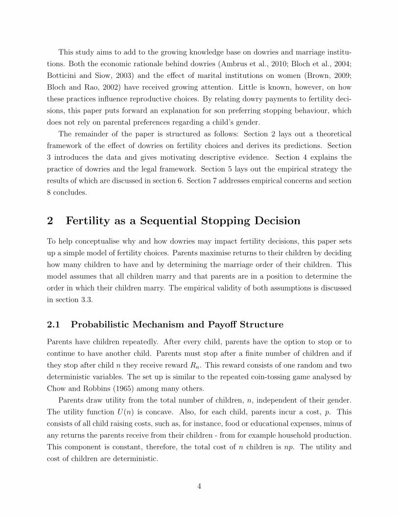
Parents draw utility from the total number of children, n, independent of their gender.

The utility function U(n) is concave. Also, for each child, parents incur a cost, p. This

consists of all child raising costs, such as, for instance, food or educational expenses, minus of

any returns the parents receive from their children - from for example household production.

This component is constant, therefore, the total cost of n children is np. The utility and

cost of children are deterministic.

4

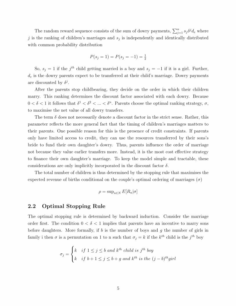
The random reward sequence consists of the sum of dowry payments,∑n

j=1 sjδjde where

j is the ranking of children’s marriages and sj is independently and identically distributed

with common probability distribution

P (sj = 1) = P (sj = −1) = 12

So, sj = 1 if the jth child getting married is a boy and sj = −1 if it is a girl. Further,

de is the dowry parents expect to be transferred at their child’s marriage. Dowry payments

are discounted by δj.

After the parents stop childbearing, they decide on the order in which their children

marry. This ranking determines the discount factor associated with each dowry. Because

0 < δ < 1 it follows that δ1 < δ2 < ... < δn. Parents choose the optimal ranking strategy, σ,

to maximise the net value of all dowry transfers.

The term δ does not necessarily denote a discount factor in the strict sense. Rather, this

parameter reflects the more general fact that the timing of children’s marriages matters to

their parents. One possible reason for this is the presence of credit constraints. If parents

only have limited access to credit, they can use the resources transferred by their sons’s

bride to fund their own daughter’s dowry. Thus, parents influence the order of marriage

not because they value earlier transfers more. Instead, it is the most cost effective strategy

to finance their own daughter’s marriage. To keep the model simple and tractable, these

considerations are only implicitly incorporated in the discount factor δ.

The total number of children is thus determined by the stopping rule that maximises the

expected revenue of births conditional on the couple’s optimal ordering of marriages (σ)

ρ = supn∈N E[Rn|σ]

2.2 Optimal Stopping Rule

The optimal stopping rule is determined by backward induction. Consider the marriage

order first. The condition 0 < δ < 1 implies that parents have an incentive to marry sons

before daughters. More formally, if b is the number of boys and g the number of girls in

family i then σ is a permutation on 1 to n such that σj = k if the kth child is the jth boy

σj =

k if 1 ≤ j ≤ b and kth child is jth boy

k if b+ 1 ≤ j ≤ b+ g and kth is the (j − b)thgirl

5

The optimal stopping rule for reproductive choices is that parents have another child

as long as the expected benefits of doing so exceed the expected costs. For parents with n

children ρ is

U ′(n)− p+ ED ≥ 0 (1)

where the utility from another child is U ′(n) = U(n+ 1)−U(n), p the marginal cost and

ED the expected change in dowry transfers resulting from another child. The latter term

is the sum of expected dowry payments after n + 1 births minus dowry payments after n

births. Hence, ED = E(∑n+1

j=1 sjδjde)−

∑nj=1 sjδ

jde.

To formalise ED, consider family i with b boys and g girls. For this family net dowry

payments are

b∑j=1

δjde −b+g∑

j=b+1

δjde (2)

The expected dowry of another birth is

1

2(b+1∑j=1

δjde −b+g+1∑j=b+2

δjde) +1

2(

b∑j=1

δjde −b+g+1∑j=b+1

δjde)

=b∑

j=1

δjde −b+g+1∑j=b+2

δjde (3)

The expected change in dowry, ED, is the difference between equations 3 and 2, which

simplifies to

ED = deδb+1(1− δg) (4)

Thus, reformulating equation 1, parents will have another birth if the following inequality

holds

U ′(n)− p+ deδb+1(1− δg) ≥ 0 (5)

which clearly shows that the expected benefits from another birth depend on the gender

composition of children alive. Note that with zero dowry payments (de = 0), equation

5 simplifies to the standard marginal equality condition postulated by the Becker-Lewis

(1973) model.

Intuitively, the model presented here can be seen as follows. The expected revenue of a

daughter does not depend on the gender composition of children in the family. Optimising

6

parents marry the youngest daughter after all other children. The expected revenue of a son,

by contrast, increases with the number of girls already in the family. Families with many

daughters face higher dowry payments (net of dowry receipts) in the future. These families

would benefit disproportionately from the resources received as the result of marrying a son.

2.3 Testable Implications

The framework laid out in sections 2.1 and 2.2 gives rise to two implications regarding

the relation between dowries and fertility decisions: (i) at every birth order there exists a

positive correlation between the number of daughters in the family and the propensity to

have another child. Consider equation 5, since 0 < δ < 1, as g increases (1 − δg) increases

and so does ED. Thus, the higher the number of girls in the family (conditional on the

total number of children), the higher the expected benefits from another birth. This leads to

higher birth rates. The positive correlation between female offspring and fertility rates has

been widely documented (see Das Gupta et al., 2003; for instance). The second implication

is that: (ii) the correlation mentioned in point (i) is increasing in the expected dowries, de.

This can be seen from the functional form of ED where de enters multiplicatively.

To illustrate implications (i) and (ii), consider two families with k children. Family A

with bA boys and gA girls and family B with bB boys and gB girls.4 Without loss of generality

assume gA > gB. Because k is held constant, the expected future dowry transfers of another

birth are respectively

ED(A) = deδk+1(δgA − 1) (6)

ED(B) = deδk+1(δgB − 1) (7)

subtracting equation 6 from 7 yields deδk+1(δ−gA − δ−gB). Since the assumption was

that gA > gB, then δ−gA < δ−gB which implies that ED(A) > ED(B). This confirms (i).

Furthermore the difference between 6 from 7 becomes larger for increasing values of de,

therefore, (ii) follows.

3 Data and Summary Statistics

This paper is motivated by two facts: women report a higher ideal number of sons than

daughters and families with more girls than boys have above average fertility rates.

4Because the number of children is equal, the marginal utility and price of the next birth is the same forboth families. These two terms are hence omitted from this illustration.

7

3.1 The Data

This study employs data drawn from three rounds of the National Family Health Survey

(NFHS) for India (NFHS-1, NFHS-2 and NFHS-3), a nationally representative survey of

Indian households. The NFHS is part of the Demographic and Health Surveys series, which

is conducted in about 70 low and middle income countries around the world.5 The question-

naires collect extensive information on health, nutrition and the complete birth histories of

interviewed women. The NFHS-1 (IIPS 1994) was carried out in 1992 and 1993 and inter-

viewed 89,777 ever-married women aged 13 to 49; the NFHS-2 (IIPS 1999) was conducted in

1998 and 1999 and interviewed 89,199 ever married women aged 15 to 49; finally the NFHS-3

(IIPS 2007b) was implemented in 2005 and 2006 and interviewed 124,385 women aged 15 to

49.

Individuals selected for estimation are women, who have experienced at least one birth

and who have come to the end of their reproductive years, i.e. aged 36 or above. Although

biologically women can still conceive in their late 30s and early 40s, the percentage of women

doing so in India is very low. The NFHS-3 final report (NFHS, 2007a) indicates that fertility

at ages 35 and above accounts for only 4 percent of total fertility in urban and 7 percent

in rural areas. The relatively low age cut off used here is chosen to keep sample sizes large

enough for the sub-group analysis carried out in section 6.2.2.6 Similarly, the omission of

childless women is unlikely to bias the results significantly, only 4 percent of women aged 35

to 40 in India have never experienced a birth (NFHS-3, 2007a). The final sample consists

of 412,378 children of 99,533 mothers, who were born between the years 1942 and 1970.

Women in the sample show relatively low levels of education, around half of the individuals

have completed primary school. The majority are Hindu (85 percent) with a minority of

Muslim women (11 percent). Around 15 percent belong to a scheduled caste.

3.2 The Sample and Summary Statistics

Individuals in the sample have given birth to, on average, 4.1 children. The mean age at

first birth is around 20 years. The mode of the distribution lies at 3 children. Most women

have between 2 and 5 children, the percentages of mothers with 2, 3, 4 and 5 children are 18,

22, 19 and 14 percent respectively. The gender composition of offspring is relatively close to

the natural rate; 47.8 percent of children born to women are female.7

The NFHS elicits retrospective questions on respondents’ ideal number of children, sons

5The data are publicly available at measuredhs.com6Restricting the sample to women aged 40 and above does not alter the results significantly.7The natural rate of girls born at birth is 48.8 percent.

8

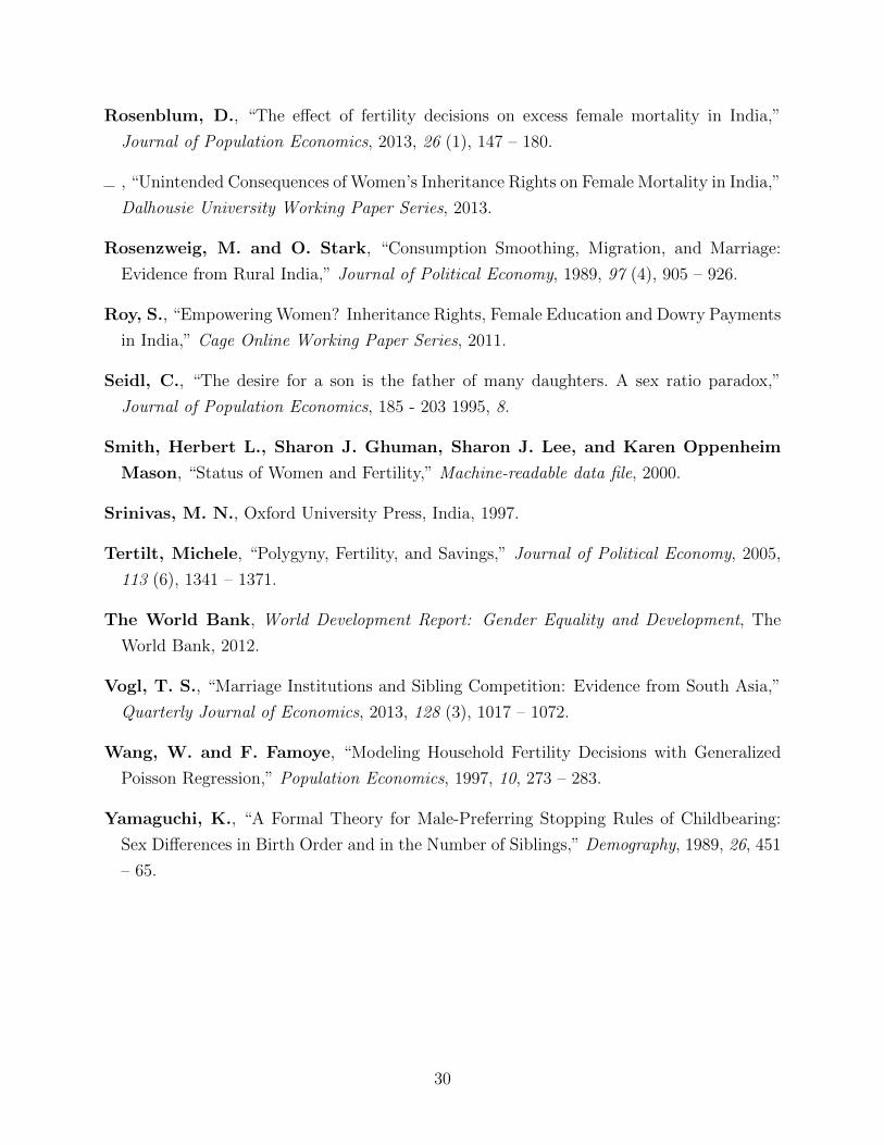
and daughters.8 Individuals in the sample report an ideal number of 2.8 children, 1.4 sons

and 1.1 daughters.9 Figure 1 plots the mean of the ideal number of children, boys and girls as

well as the difference between the latter two by the birth year of the mother. For all cohorts,

the ideal number of sons exceeds the ones of daughters by around 0.4. This difference appears

remarkably stable over time. Whilst the ideal number of children decreases from 3.3. to 2.5,

the difference between ideal sons and daughters goes down relatively little, from 0.5 to 0.3.

From an intuitive point of view, the effect of preferences for sons on fertility is ambiguous.

If son preferences manifest themselves as an aversion of girls (Diamond-Smith et al., 2008),

families with more daughters decrease fertility to avoid another female birth. If, on the

other hand, son preferences are reflected as a desire to have at least as many boys as girls

in the household, parents with many daughters increase their fertility in the hope of male

births. Descriptive evidence from the NFHS supports the latter. Figure 2 reports the

correlations between the gender compositions of children and their parents’ fertility rates.

The base category are parents with an equal amount of sons and daughters.10 Compared to

these individuals, families with more daughters have higher fertility levels. The conditional

probability of another birth increases by 10 percentage points for families with only girls

and by 3 percentage points for families with more girls than boys. The correlation between

the number of boys and fertility, by contrast, is ambiguous. Families with only sons have a

6 percentage point higher probability to have another child. Parents with more boys than

girls, on the other hand, are 7 percentage points less likely to have another child.

3.3 Marriages in India

The theoretical model makes two assumptions about marital behaviour in India. First, all

children marry. Marriage is central to Indian social life and holds value in both Hinduism and

Islam. Evidence from the NFHS (1994) further confirms that marriage is virtually universal

in India. Only 1 percent of women aged 35 to 39 remain unmarried.

Second, parents are in a position to determine the order in which their children marry and

they attempt to marry sons before daughters. The assumption that marriage patterns of fam-

ily members are determined by the household as a whole is not uncommon (see Rosenzweig

and Stark, 1989; for instance). In fact, around the time of the introduction of the Dowry

8The relevant questions are If you could choose exactly the number of children to have in your whole life,how many would that be? and How many of these children would you like to be boys and how many girls?

9The number of ideal sons and daughters do not add up because in the second and third round of theNFHS women were also asked about their ideal number of children regardless of the sex.

10This is modelled in a regression framework where the dependent variable takes the value 1 if the womanexperiences another birth. The controls include the total number of children born, a time trend and motherlevel unobserved heterogeneity.

9

Prohibition Rules, most marriages in India were arranged (Dixon, 1971). The short birth

intervals commonly observed in India further facilitate the marriage of sons before daughters.

Figures from the NFHS-1 (1994) show that the median birth interval is two years. This is

comparatively short compared to the standard deviation in the age at marriage, which is 3.5

years.

As pointed out by Vogl (2013), parents attempt to marry their children in gender specific

birth order, which implies that marriages of girls (or boys) are influenced predominantly by

the number of their older sisters (or brothers). Figure 3 shows the share of children married

by age and gender of next youngest sibling. India is a virilocal society in which, after

marriage, the bride moves to the groom and his family. Thus, the marriage of a woman are

approximated by her leaving the household whereas the marriage of a man is self reported.

The two figures suggest that women with younger sisters tend to marry earlier whereas men

are less affected by the gender of their younger sibling. These patterns are compatible with

parental incentives to marry sons before daughters.

To give more detail on marriage behaviour in India, this paper follows the methodology

by Vogl (2013) and estimates the probability of a child marrying as a function of individual

controls (like age11) and the gender of younger siblings. Columns (1) and (2) of table 1

employ the gender of the next child only and suggest that the birth of a younger sister (as

compared to the birth of a younger brother) increases the probability of getting married by

3 percentage points for women and decreases the probability by 1 percentage points for men.

Columns (3) to (6) control for the total number of younger siblings and include the number of

younger sisters and brothers separately. The parameter estimates show that younger sisters

increase and younger brothers decrease the marriage probability for women. The opposite is

true for men. Like before, these parameter estimates are compatible with parental behaviour

that endeavours to marry sons before daughters.

4 Dowries in India

The custom of marital payments is widespread in India. Between 60 and 90 percent of women

interviewed in 1993 (SWAF, 1994) reported to have paid a dowry at their own marriage.

11The controls include age, birth order and state of residence fixed effects and parental education, casteand religion.

10

4.1 Evidence on Dowries

Much of the research on dowries has focused on the prevalence and value of marital payments.

From a theoretical point of view, Anderson (2003) maintains that the prevalence of dowries

in India is a result of fast economic development combined with the rigid social system

provided by the country’s caste system. Do et al. (2013) and Tertilt (2005) consider the

importance of marriage patterns; Roy (2011); Dalmia (2004); Deolalikar and Rao (1998)

focus on the characteristics of the groom, Caldwell et al. (1983) on the ones of the bride.

There is no consensus, however, on the precise monetary value of these transfers. Rao (1993,

2000) argues that dowries amount to up to 68 percent of assets before marriage. Other

research, by contrast, has put forward much lower figures (Arunachalam and Logan, 2008;

Anderson, 2007b; Edlund, 2000). In particular, Edlund (2006) distinguishes gross from net

dowry payments and argues that the increase in net dowries has been negligible.

A commonly used source of information on dowry transfers is the survey carried out by

the International Crops Research Institute for the Semi-Arid Tropics (ICRISAT). The survey

is carried out in 6 different villages in the Indian state of Andhra Pradesh between the years

1975 and 1984. This survey contains self-reported information on, inter alia, age, marital

status of all household members and inventory files for current physical stocks as well as on

financial assets and liabilities such as bank accounts and dowries. Table 2 reports average

dowries paid and received by households using ICRISAT data. The majority of households

report to have either paid or received a dowry, 81 percent in column (1). Rows (b) and (c)

report the dowries paid, (d) and (e) dowries received and (f) and (g) the net out payments

per household.12 For the whole sample, households pay larger amount of dowries than they

receive, 1,584 Rupees versus 600 Rupees per annum. The 684 Rupees per year net payments

translate into around 70 Rupees per person residing in the household per year.13 A possible

reason for this disparity that parents can only capture part of the dowry given to their sons.

Dowries make up more than half of the household’s non-durable consumption expenditures,

see row (h), and 8 percent of the income of all household members combined see row (i).

4.2 Dowry Laws in India

In an attempt to curb the prevalence of dowries, the government of India passed the Dowry

Prohibition Act in 1961 prohibiting the giving and taking of dowry (Dowry Prohibition Act,

1961).14 Despite this legislation few dowry cases reached the courts and the practice of

12These are defined as the dowries paid minus the dowries received by the household.13All numbers are given in 1984 Rupees. Official GDP per capita in 1980 was Rupees 1,630.14Dowry is defined as ”any property or valuable security given or agreed to be given either directly or

indirectly a) by one party to a marriage to the other party to the marriage or b) by the parents of either

11

dowries persisted (see evidence in section 4.1). A common reason put forward for this is

that the 1961 Act’s provisions were not strong enough to implement successful prosecutions

(Chowdhary, 1998).

In response to this, the government of India introduced the Dowry Prohibition Rules

(1985),15 which are the focus of this empirical analysis. The purpose of this amendment was

to make the Dowry Prohibition Act of 1961 more stringent and effective in a number of ways.

First, the legislation establishes a set of rules in accordance with which a list of presents has

to be maintained. The list of presents given to be bride is kept by the bride whereas the list

containing presents to the groom is kept with the groom. These lists must be in writing and

contain the approximate value of the present. Second, the Dowry Prohibition Rules raise the

minimum punishment for taking or abetting the taking of dowry to 5 years of imprisonment

and to a fine of 15,000 Rupees. Third, the burden of proving that no funds were exchanged

now lies with the person who takes or abets the taking of dowry. Fourth, offences to the act

are made non-bailable.

To facilitate the implementation of the newly established rules, the amended act intro-

duced the Dowry Prohibition Officers. The tasks of these public sector employees included

the prevention of the taking and demanding of dowries and the collection of evidence neces-

sary for the prosecution of persons committing offences under the Dowry Prohibition Act.16

Legal research has pointed to a marked increase in dowry cases heard by courts in the mid

1980s (Menksi, 1998). Furthermore, India’s high court took a much stricter approach to

dowry offenders. Overall, the new rules were perceived by many as countering the prevalent

attitude of patriarchal traditions that women were owned by men.

4.3 The Impact of the Dowry Prohibition Rules

Evidence from the Survey if Status of Women (2000) suggests that the Dowry Prohibition

Rules had a marked effect on dowry transfers. The SWAF is part of a series implemented

in India, Malaysia, Pakistan, the Philippines and Thailand. The questionnaire was carried

out in 1993 and 1994 in four districts in the states of Tamil Nadu and Uttar Pradesh. It

interviewed 1,600 women in total. The survey collected information on current health and

different dimensions of female autonomy as well as retrospective information on marriages

and dowry transfers.17

Figure 4 reports the differences in the conditional probability of a dowry being paid at

party to a marriage or by any other person to either part to the marriage or to any other person at or beforeor any time after the marriage in connection with the marriage of said parties”

15Amendment Act 63 of 1984 came into force on the 2.10.1985.16Section 8B of the amended Dowry Prohibition Act.17The data are publicly available at swap.pop.upenn.edu/datasets

12

a woman’s marriage between the years 1970 and 1994.18 Whilst the conditional probability

estimates of dowry payments in the years leading up to the policy are very similar, around

12% to 16% lower than the base years, the estimates drop to -30% in 1985. In subsequent

years, the probability estimates oscillate between -30% and -40% before eventually dropping

to -60% for the last year, 1992. This final drop may have been caused by the gradual

introduction of the Dowry Prohibition Officers. As mentioned, the 1985 law stipulated the

creation of these new public sector employees and it is likely that their impact was delayed. It

is unlikely that this drop is the result of respondents misreporting their dowry transfers. As

previously mentioned, the questions about dowries were asked to all women retrospectively

in 1993 and 1994. Hence, whilst respondents may have had an incentive to misreport in

general, it is unlikely that this incentive varied according to whether they married before or

after the policy change.

Further descriptive evidence from the SWAF suggests that the change in policy affected

parents’ expectations of a dowry being paid. One question concerns mothers and the dowries

they expect to pay. Figure 5 shows the percentage of mothers expecting to pay a dowry by

the year of the last born child. The percentage of women intending to pay a dowry increases

for birth years before the introduction of the policy. These individuals are more likely to have

heard of the policy. For children born after the policy, by contrast, the fraction decreases.

However, since the sample includes women that have not yet completed their childbearing

years, this trend may reflect inexperience regarding dowry issues. Hence, the evidence is

only to be seen as suggestive.

5 Empirical Strategy

This paper exploits the exogenous decrease in expected dowries resulting from the Dowry

Prohibition Rules outlined above to test implications (i) and (ii) empirically.

5.1 Empirical Framework

This paper investigates the probability that a woman gives birth after a given number of

children. This probability is estimated as a function of individual controls and the gender

composition of her offspring. The study constructs complete, retrospective birth histories.

Thus, each mother contributes J+1 observations where J is the total number of births experi-

enced in her lifetime; one for every birth she experiences with the addition of one observation

18The base years are 1966 to 1972. Covariates include the years of birth of the two members of the couple,their education, their parental background and a village level fixed effect.

13

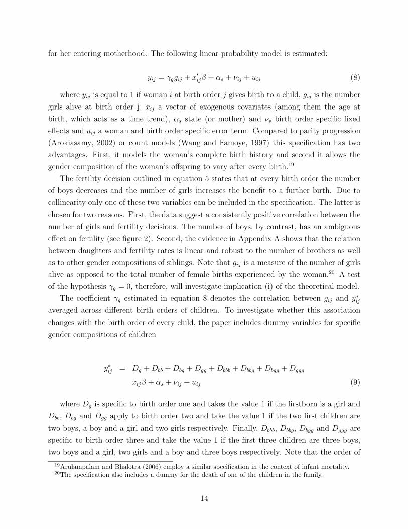
for her entering motherhood. The following linear probability model is estimated:

yij = γggij + x′ijβ + αs + νij + uij (8)

where yij is equal to 1 if woman i at birth order j gives birth to a child, gij is the number

girls alive at birth order j, xij a vector of exogenous covariates (among them the age at

birth, which acts as a time trend), αs state (or mother) and νs birth order specific fixed

effects and uij a woman and birth order specific error term. Compared to parity progression

(Arokiasamy, 2002) or count models (Wang and Famoye, 1997) this specification has two

advantages. First, it models the woman’s complete birth history and second it allows the

gender composition of the woman’s offspring to vary after every birth.19

The fertility decision outlined in equation 5 states that at every birth order the number

of boys decreases and the number of girls increases the benefit to a further birth. Due to

collinearity only one of these two variables can be included in the specification. The latter is

chosen for two reasons. First, the data suggest a consistently positive correlation between the

number of girls and fertility decisions. The number of boys, by contrast, has an ambiguous

effect on fertility (see figure 2). Second, the evidence in Appendix A shows that the relation

between daughters and fertility rates is linear and robust to the number of brothers as well

as to other gender compositions of siblings. Note that gij is a measure of the number of girls

alive as opposed to the total number of female births experienced by the woman.20 A test

of the hypothesis γg = 0, therefore, will investigate implication (i) of the theoretical model.

The coefficient γg estimated in equation 8 denotes the correlation between gij and y∗ij

averaged across different birth orders of children. To investigate whether this association

changes with the birth order of every child, the paper includes dummy variables for specific

gender compositions of children

y∗ij = Dg +Dbb +Dbg +Dgg +Dbbb +Dbbg +Dbgg +Dggg

xijβ + αs + νij + uij (9)

where Dg is specific to birth order one and takes the value 1 if the firstborn is a girl and

Dbb, Dbg and Dgg apply to birth order two and take the value 1 if the two first children are

two boys, a boy and a girl and two girls respectively. Finally, Dbbb, Dbbg, Dbgg and Dggg are

specific to birth order three and take the value 1 if the first three children are three boys,

two boys and a girl, two girls and a boy and three boys respectively. Note that the order of

19Arulampalam and Bhalotra (2006) employ a similar specification in the context of infant mortality.20The specification also includes a dummy for the death of one of the children in the family.

14

children is not considered here. The estimation of equation 9 only considers children born

at birth order four or less.

5.2 Difference-in-differences specification

Implication (ii) of the theoretical model states that a decrease in de attenuates the positive

correlation between the number of girls and fertility (see equation 5). In the reduced form

equation, this correlation is denoted by γg (see equation 8). Thus, we would expect the

introduction of the Dowry Prohibition Rules to decrease the parameter estimate of γg. The

paper investigates this hypothesis by estimating a difference-in-differences model, which also

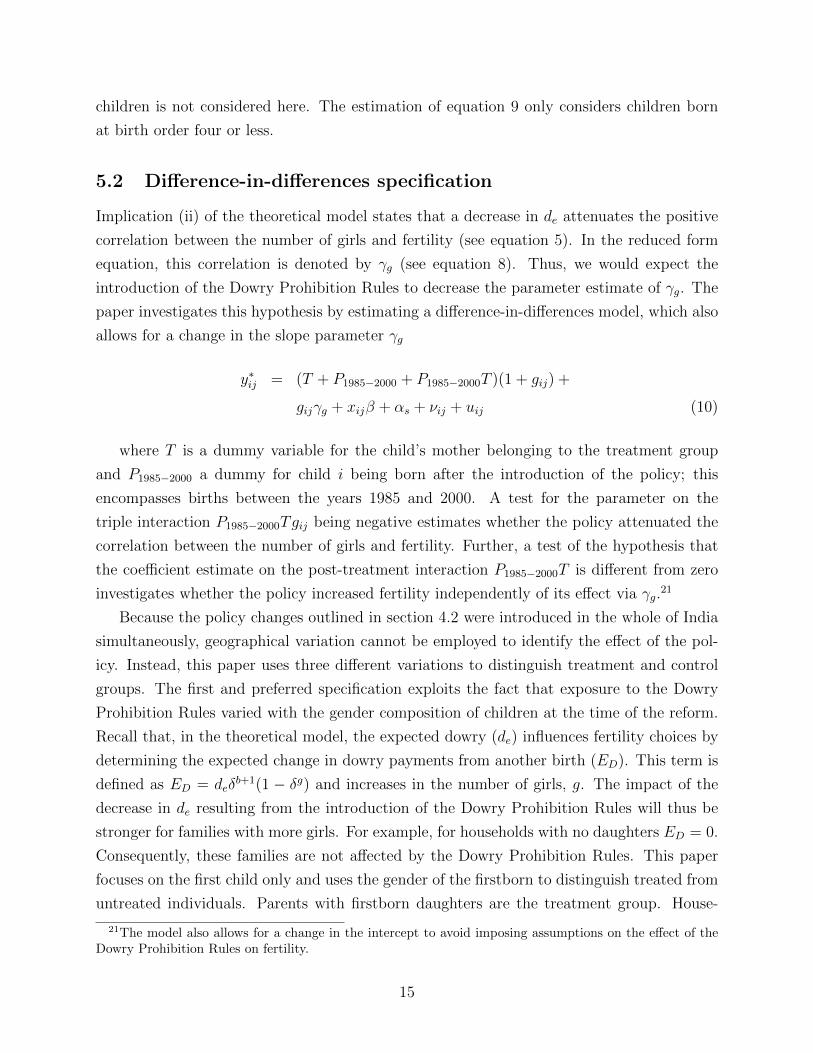
allows for a change in the slope parameter γg

y∗ij = (T + P1985−2000 + P1985−2000T )(1 + gij) +

gijγg + xijβ + αs + νij + uij (10)

where T is a dummy variable for the child’s mother belonging to the treatment group

and P1985−2000 a dummy for child i being born after the introduction of the policy; this

encompasses births between the years 1985 and 2000. A test for the parameter on the

triple interaction P1985−2000Tgij being negative estimates whether the policy attenuated the

correlation between the number of girls and fertility. Further, a test of the hypothesis that

the coefficient estimate on the post-treatment interaction P1985−2000T is different from zero

investigates whether the policy increased fertility independently of its effect via γg.21

Because the policy changes outlined in section 4.2 were introduced in the whole of India

simultaneously, geographical variation cannot be employed to identify the effect of the pol-

icy. Instead, this paper uses three different variations to distinguish treatment and control

groups. The first and preferred specification exploits the fact that exposure to the Dowry

Prohibition Rules varied with the gender composition of children at the time of the reform.

Recall that, in the theoretical model, the expected dowry (de) influences fertility choices by

determining the expected change in dowry payments from another birth (ED). This term is

defined as ED = deδb+1(1 − δg) and increases in the number of girls, g. The impact of the

decrease in de resulting from the introduction of the Dowry Prohibition Rules will thus be

stronger for families with more girls. For example, for households with no daughters ED = 0.

Consequently, these families are not affected by the Dowry Prohibition Rules. This paper

focuses on the first child only and uses the gender of the firstborn to distinguish treated from

untreated individuals. Parents with firstborn daughters are the treatment group. House-

21The model also allows for a change in the intercept to avoid imposing assumptions on the effect of theDowry Prohibition Rules on fertility.

15

holds, whose firstborn is male, are the control group. The exogeneity of the firstborn’s gender

is investigated in section B.

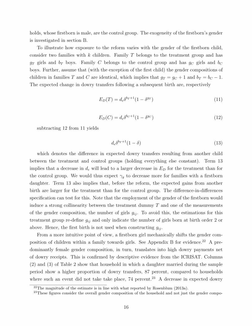
To illustrate how exposure to the reform varies with the gender of the firstborn child,

consider two families with k children. Family T belongs to the treatment group and has

gT girls and bT boys. Family C belongs to the control group and has gC girls and bC

boys. Further, assume that (with the exception of the first child) the gender compositions of

children in families T and C are identical, which implies that gT = gC + 1 and bT = bC − 1.

The expected change in dowry transfers following a subsequent birth are, respectively

ED(T ) = deδbT+1(1− δgT ) (11)

ED(C) = deδbC+1(1− δgC ) (12)

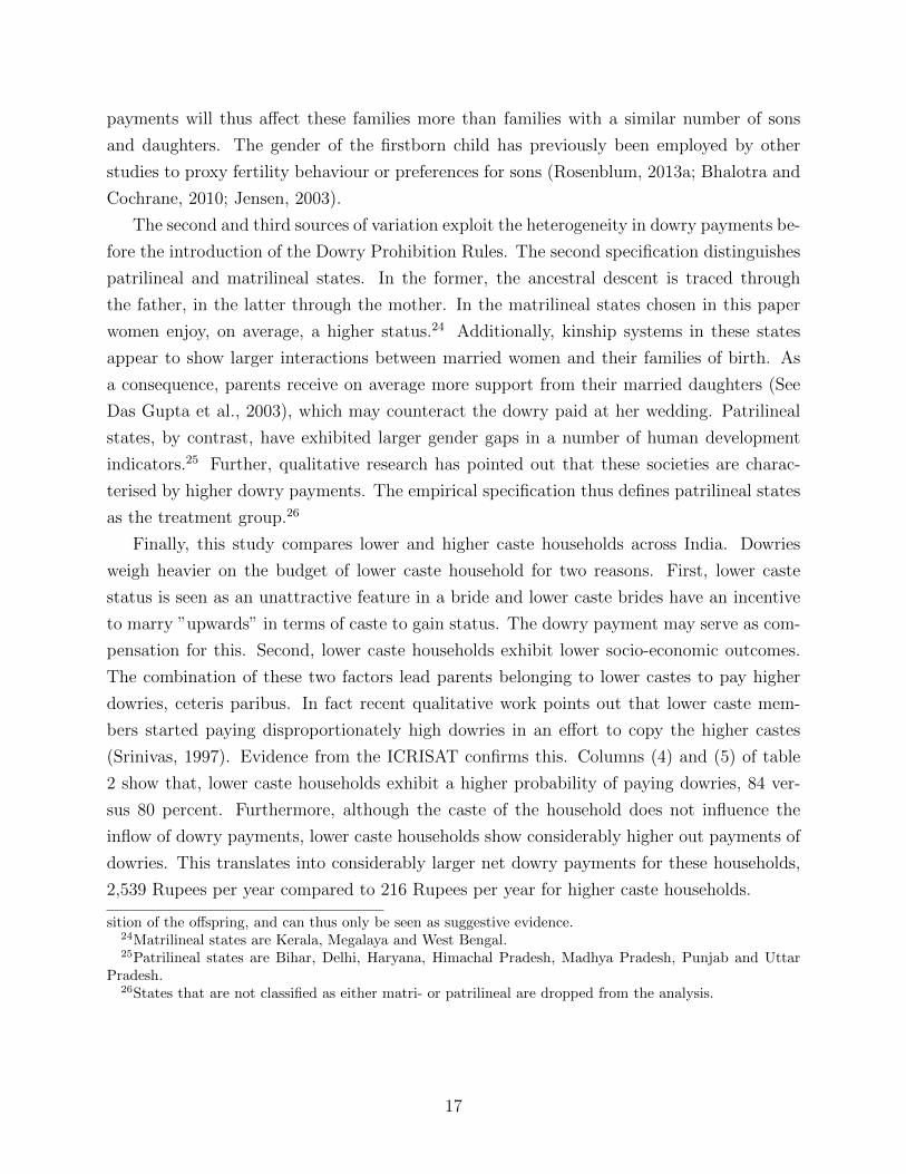
subtracting 12 from 11 yields

deδbT+1(1− δ) (13)

which denotes the difference in expected dowry transfers resulting from another child

between the treatment and control groups (holding everything else constant). Term 13

implies that a decrease in de will lead to a larger decrease in ED for the treatment than for

the control group. We would thus expect γg to decrease more for families with a firstborn

daughter. Term 13 also implies that, before the reform, the expected gains from another

birth are larger for the treatment than for the control group. The difference-in-differences

specification can test for this. Note that the employment of the gender of the firstborn would

induce a strong collinearity between the treatment dummy T and one of the measurements

of the gender composition, the number of girls gij. To avoid this, the estimations for this

treatment group re-define gij and only indicate the number of girls born at birth order 2 or

above. Hence, the first birth is not used when constructing gij.

From a more intuitive point of view, a firstborn girl mechanically shifts the gender com-

position of children within a family towards girls. See Appendix B for evidence.22 A pre-

dominantly female gender composition, in turn, translates into high dowry payments net

of dowry receipts. This is confirmed by descriptive evidence from the ICRISAT. Columns

(2) and (3) of Table 2 show that household in which a daughter married during the sample

period show a higher proportion of dowry transfers, 87 percent, compared to households

where such an event did not take take place, 74 percent.23 A decrease in expected dowry

22The magnitude of the estimate is in line with what reported by Rosenblum (2013a).23These figures consider the overall gender composition of the household and not just the gender compo-

16

payments will thus affect these families more than families with a similar number of sons

and daughters. The gender of the firstborn child has previously been employed by other

studies to proxy fertility behaviour or preferences for sons (Rosenblum, 2013a; Bhalotra and

Cochrane, 2010; Jensen, 2003).

The second and third sources of variation exploit the heterogeneity in dowry payments be-

fore the introduction of the Dowry Prohibition Rules. The second specification distinguishes

patrilineal and matrilineal states. In the former, the ancestral descent is traced through

the father, in the latter through the mother. In the matrilineal states chosen in this paper

women enjoy, on average, a higher status.24 Additionally, kinship systems in these states

appear to show larger interactions between married women and their families of birth. As

a consequence, parents receive on average more support from their married daughters (See

Das Gupta et al., 2003), which may counteract the dowry paid at her wedding. Patrilineal

states, by contrast, have exhibited larger gender gaps in a number of human development

indicators.25 Further, qualitative research has pointed out that these societies are charac-

terised by higher dowry payments. The empirical specification thus defines patrilineal states

as the treatment group.26

Finally, this study compares lower and higher caste households across India. Dowries

weigh heavier on the budget of lower caste household for two reasons. First, lower caste

status is seen as an unattractive feature in a bride and lower caste brides have an incentive

to marry ”upwards” in terms of caste to gain status. The dowry payment may serve as com-

pensation for this. Second, lower caste households exhibit lower socio-economic outcomes.

The combination of these two factors lead parents belonging to lower castes to pay higher

dowries, ceteris paribus. In fact recent qualitative work points out that lower caste mem-

bers started paying disproportionately high dowries in an effort to copy the higher castes

(Srinivas, 1997). Evidence from the ICRISAT confirms this. Columns (4) and (5) of table

2 show that, lower caste households exhibit a higher probability of paying dowries, 84 ver-

sus 80 percent. Furthermore, although the caste of the household does not influence the

inflow of dowry payments, lower caste households show considerably higher out payments of

dowries. This translates into considerably larger net dowry payments for these households,

2,539 Rupees per year compared to 216 Rupees per year for higher caste households.

sition of the offspring, and can thus only be seen as suggestive evidence.24Matrilineal states are Kerala, Megalaya and West Bengal.25Patrilineal states are Bihar, Delhi, Haryana, Himachal Pradesh, Madhya Pradesh, Punjab and Uttar

Pradesh.26States that are not classified as either matri- or patrilineal are dropped from the analysis.

17

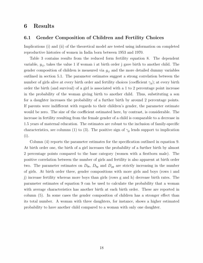
6 Results

6.1 Gender Composition of Children and Fertility Choices

Implications (i) and (ii) of the theoretical model are tested using information on completed

reproductive histories of women in India born between 1953 and 1970.

Table 3 contains results from the reduced form fertility equation 8. The dependent

variable, yij, takes the value 1 if woman i at birth order j gave birth to another child. The

gender composition of children is measured via gij and the more detailed dummy variables

outlined in section 5.1. The parameter estimates suggest a strong correlation between the

number of girls alive at every birth order and fertility choices (coefficient γg); at every birth

order the birth (and survival) of a girl is associated with a 1 to 2 percentage point increase

in the probability of the woman giving birth to another child. Thus, substituting a son

for a daughter increases the probability of a further birth by around 2 percentage points.

If parents were indifferent with regards to their children’s gender, the parameter estimate

would be zero. The size of the coefficient estimated here, by contrast, is considerable. The

increase in fertility resulting from the female gender of a child is comparable to a decrease in

1.5 years of maternal education. The estimates are robust to the inclusion of family-specific

characteristics, see columns (1) to (3). The positive sign of γg lends support to implication

(i).

Column (4) reports the parameter estimates for the specification outlined in equation 9.

At birth order one, the birth of a girl increases the probability of a further birth by almost

2 percentage points compared to the base category (women with a firstborn male). The

positive correlation between the number of girls and fertility is also apparent at birth order

two. The parameter estimates on Dbb, Dbg and Dgg are strictly increasing in the number

of girls. At birth order three, gender compositions with more girls and boys (rows i and

j) increase fertility whereas more boys than girls (rows g and h) decrease birth rates. The

parameter estimates of equation 9 can be used to calculate the probability that a woman

with average characteristics has another birth at each birth order. These are reported in

column (5). In some cases the gender composition of children has a stronger effect than

its total number. A woman with three daughters, for instance, shows a higher estimated

probability to have another child compared to a woman with only one daughter.

18

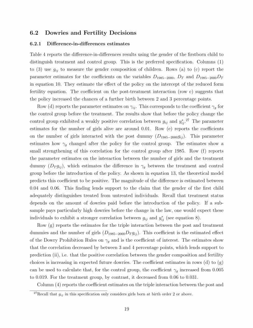
6.2 Dowries and Fertility Decisions

6.2.1 Difference-in-differences estimates

Table 4 reports the difference-in-differences results using the gender of the firstborn child to

distinguish treatment and control group. This is the preferred specification. Columns (1)

to (3) use gij to measure the gender composition of children. Rows (a) to (c) report the

parameter estimates for the coefficients on the variables D1985−2000, DT and D1985−2000DT

in equation 10. They estimate the effect of the policy on the intercept of the reduced form

fertility equation. The coefficient on the post-treatment interaction (row c) suggests that

the policy increased the chances of a further birth between 2 and 3 percentage points.

Row (d) reports the parameter estimates on γij. This corresponds to the coefficient γg for

the control group before the treatment. The results show that before the policy change the

control group exhibited a weakly positive correlation between gij and y∗ij.27 The parameter

estimates for the number of girls alive are around 0.01. Row (e) reports the coefficients

on the number of girls interacted with the post dummy (D1985−2000gij). This parameter

estimates how γg changed after the policy for the control group. The estimates show a

small strengthening of this correlation for the control group after 1985. Row (f) reports

the parameter estimates on the interaction between the number of girls and the treatment

dummy (DTgij), which estimates the difference in γg between the treatment and control

group before the introduction of the policy. As shown in equation 13, the theoretical model

predicts this coefficient to be positive. The magnitude of the difference is estimated between

0.04 and 0.06. This finding lends support to the claim that the gender of the first child

adequately distinguishes treated from untreated individuals. Recall that treatment status

depends on the amount of dowries paid before the introduction of the policy. If a sub-

sample pays particularly high dowries before the change in the law, one would expect these

individuals to exhibit a stronger correlation between gij and y∗ij (see equation 8).

Row (g) reports the estimates for the triple interaction between the post and treatment

dummies and the number of girls (D1985−2000DTgij). This coefficient is the estimated effect

of the Dowry Prohibition Rules on γg and is the coefficient of interest. The estimates show

that the correlation decreased by between 3 and 4 percentage points, which lends support to

prediction (ii), i.e. that the positive correlation between the gender composition and fertility

choices is increasing in expected future dowries. The coefficient estimates in rows (d) to (g)

can be used to calculate that, for the control group, the coefficient γg increased from 0.005

to 0.019. For the treatment group, by contrast, it decreased from 0.06 to 0.031.

Column (4) reports the coefficient estimates on the triple interaction between the post and

27Recall that gij in this specification only considers girls born at birth order 2 or above.

19

treatment dummies on the one hand and the dummies for the gender compositions outlined

in equation 9 on the other.28 The figures suggest that the decrease in the correlation between

the gender composition of children and fertility was strongest at birth orders three and four.

At birth order three the coefficient for couples with one boy and one girl decreased by 4

percentage points. Similarly, at birth order 4, the coefficient for families with two girls and

one boy decreased by 6 percentage points. The correlation for birth order 2, by contrast,

increased as a result of the policy.

Table 5 reports the difference-in-differences estimates employing two alternative specifi-

cations to distinguish the treatment and control group. Columns (1), (2) and (3) compare

patri-lineal (the treatment group) and matri-lineal states (the control group). The results

are similar to the ones outlined in the main specification. The Dowry Prohibition Rules are

estimated to increase the intercept of the fertility equation by between 6 and 8 percentage

points. These magnitudes exceed the ones of table 4. For the control group the number

of girls appears to have a weaker correlation to fertility choices. This has intuitive appeal;

matri-lineal states place high importance on daughters and have been documented to pay

lower dowries. It is, therefore, unlikely that these states exhibit strong son preferences in

fertility behaviour. The estimates in row (d) show that also for this specification the policy

decreased the correlation between the number of girls and fertility by around 3 percentage

points. Columns (4), (5) and (6) report the parameter estimates comparing families of low

castes (the treatment group) with high caste individuals (the control group). Akin to before,

the estimates are in line with the ones reported in table 4 and the ones reported in columns

(1) to (3). For this specification, the reform is estimated to have decreased the correlation

between girls and fertility by around 2 percentage points.

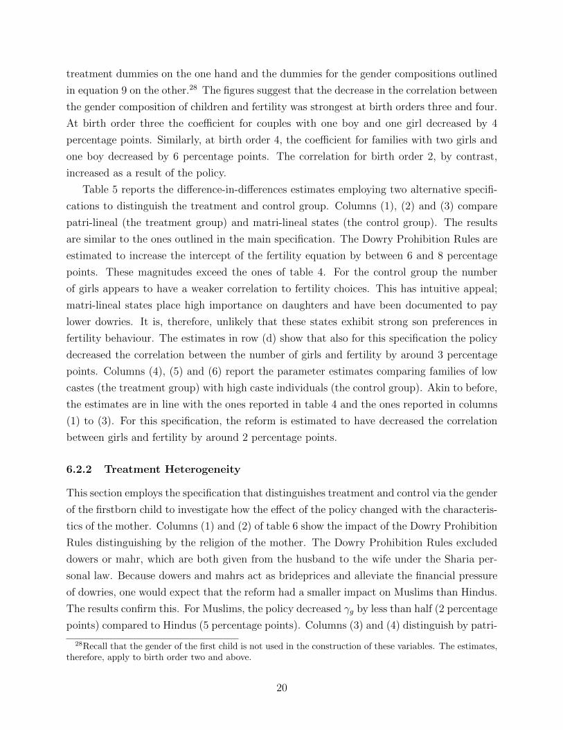
6.2.2 Treatment Heterogeneity

This section employs the specification that distinguishes treatment and control via the gender

of the firstborn child to investigate how the effect of the policy changed with the characteris-

tics of the mother. Columns (1) and (2) of table 6 show the impact of the Dowry Prohibition

Rules distinguishing by the religion of the mother. The Dowry Prohibition Rules excluded

dowers or mahr, which are both given from the husband to the wife under the Sharia per-

sonal law. Because dowers and mahrs act as brideprices and alleviate the financial pressure

of dowries, one would expect that the reform had a smaller impact on Muslims than Hindus.

The results confirm this. For Muslims, the policy decreased γg by less than half (2 percentage

points) compared to Hindus (5 percentage points). Columns (3) and (4) distinguish by patri-

28Recall that the gender of the first child is not used in the construction of these variables. The estimates,therefore, apply to birth order two and above.

20

and matri-lineal states. As mentioned before, dowries are more pronounced in patri-lineal

states and the results show that the effect of the policy in these states is more pronounced (5

percentage points) compared to matri-lineal states (2 percentage points). Columns (5) and

(6), moreover, suggest a clear positive correlation between the impact of the Dowry Prohibi-

tion Rules and the mother’s education. The slope parameter for the former group decreases

by 5 percentage points whereas for the latter it is only attenuated by 4 percentage points.

One possible explanation for this finding is that women with higher levels of education are

likely to have higher levels of autonomy. The resulting improved agency is likely to enable

these individuals to respond more effectively to the new circumstances by affecting decisions

taken by the household as a whole. Columns (7) to (10) employ two different variables that

have previously been used as proxies for female autonomy: age and age difference at mar-

riage (Abadian, 1996). The results confirm that more autonomous women responded more

strongly to the Dowry Prohibition Rules.

7 Identification Concerns

The key identifying assumption of the difference-in-differences estimator is that the time

trend in reproductive behaviour would have been the same for treatment and control group

in the absence of the reform. This sub-section assesses the plausibility of this assumption in

the present context.

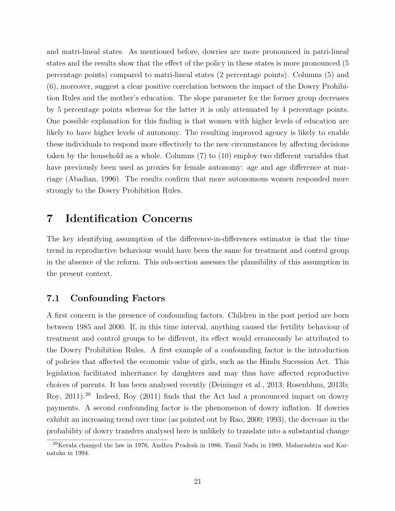
7.1 Confounding Factors

A first concern is the presence of confounding factors. Children in the post period are born

between 1985 and 2000. If, in this time interval, anything caused the fertility behaviour of

treatment and control groups to be different, its effect would erroneously be attributed to

the Dowry Prohibition Rules. A first example of a confounding factor is the introduction

of policies that affected the economic value of girls, such as the Hindu Sucession Act. This

legislation facilitated inheritance by daughters and may thus have affected reproductive

choices of parents. It has been analysed recently (Deininger et al., 2013; Rosenblum, 2013b;

Roy, 2011).29 Indeed, Roy (2011) finds that the Act had a pronounced impact on dowry

payments. A second confounding factor is the phenomenon of dowry inflation. If dowries

exhibit an increasing trend over time (as pointed out by Rao, 2000; 1993), the decrease in the

probability of dowry transfers analysed here is unlikely to translate into a substantial change

29Kerala changed the law in 1976, Andhra Pradesh in 1986, Tamil Nadu in 1989, Maharashtra and Kar-nataka in 1994.

21

in de. A common strategy for addressing these concerns is to include state specific trends

in the estimation in equation 10. Column (1) of table 7 shows that the parameter estimates

are robust to the addition of state specific trends; the difference-in-differences parameter is

-0.038.

The paper also estimates a truncated version of equation 10 as

y∗ij = (P1985−a + T + P1985−aT )(1 + gij) +

nijγn + gijγg + xijβ + αi + uij (14)

where a = 1995, 1990, 1986, 1985. In practice, only children born between 1985 and the

cut-offs defined in a are used to identify the effect of the Dowry Prohibition Rules. Children

born after the cut-off are dropped from the analysis. This shorter time frame significantly

decreases the importance of confounding factors. It is, for instance, unlikely that other poli-

cies affected treatment and control groups differently between 1985 and 1986. Furthermore,

dowry inflation is unlikely to have changed substantively in those years. Columns (2) to (5)

of table 7 report the parameter estimates, which suggest that the results are stable to the

changes in the post period. The effect of the policy on the slope parameter remains nega-

tive. For the estimates in row (c) in columns (2) to (5) the magnitudes of the effect of policy

remain similar to the previous specification, with magnitudes between 2 and 4 percentage

points.

7.2 Sex Selective Abortions

A second concern is the introduction of prenatal sex determination techniques around the

time of the Dowry Prohibition Rules. As pointed out by Bhalotra and Cochrane (2010),

families with a firstborn daughter have a stronger incentive to abort female foetuses at birth

order two or above, which would violate the common time trend assumption.

The paper addresses this concern in three ways. First, the specification outlined in

equation 14 helps us understand the importance of sex selective abortions. Previous work

has documented that the practice of sex selective abortions increased in the 1990s (see

Arnold et al, 2002b, for instance). A treatment effect estimated for children born in 1985

(and 1986) only is thus significantly less likely to be biased by sex selective abortions. Hence,

the parameter estimates reported in table 7 can be seen as first evidence against the influence

of sex selective abortions.

The second strategy compares the sex ratios at birth for the treatment and control group

before and after the introduction of the policy. If parents respond to the Dowry Prohibition

Rules by aborting female foetuses, we would expect the sex ratio at birth to decrease for

22

the treatment group in the years after the policy. The sex ratio for the control group, by

contrast, should remain the same. Figure 6 plots the percentage of girls born in the years

before and after the introduction of the Dowry Prohibition Rules.30 In both time periods,

the differences between treatment and control group do not appear to be significant. In fact,

the only statistically significant differences between the two samples are in the years 1983

and 1989. Note that, as shown in table 7 the results are robust to using children born before

1989.

Third, this paper estimates a model similar to the one employed by Bhalotra and

Cochrane (2010) to test the hypothesis that parents adopted sex selective abortions after the

year 1985. The paper estimates the probability that a child born to woman i at birth order

j is female (wij) as a function of individual characteristics, the gender of the oldest sibling

and a dummy for whether the index child was born after the introduction of the Dowry

Prohibition Rules.

wij = P1985−2000 + T + P1985−2000T + xijβ + fs + fst+ uij (15)

where P1985−2000 is an indicator variable for the child being born after the introduction

of the policy in 1985 (and up until the year 2000), and T a dummy variable for the child’s

oldest sibling being female. The specification also includes state fixed effects and state specific

trends. A test on the interaction TP1985−2000 investigates whether the Dowry Prohibition

Rules had a significant impact on the probability of a girl being born.

Table 8 reports the parameter estimates of equation 15.31 Overall, the estimates suggest

that the policy had no significant impact on the probability of a female birth. The value of

the post-treatment interaction coefficient with and without state specific trends (columns 1

and 3) are not significant. Furthermore, the sizes of the parameter estimates are very small.

They suggest that the change in the law decreased the chances of a female birth between 0.4

and 0.7 percentage points. The specification also divides the post-period into two (columns

2 and 4). Here again, no significant effect is found. One possible reason for the difference

between the estimates presented here and the ones of Bhalotra and Cochrane (2010) may be

due to the different samples used. Whilst the authors employ births to all women in India,

this paper only uses women who had come to the end of their reproductive years and who

are born between the years 1953 and 1970.

30Because the treatment is defined along the lines of the firstborn child (the exogeneity of which hasalready been argued for in table 10) this panel only considers children of birth order 2 or above.

31The dependent variable, wij , takes the value 100 if woman i at birth order j gave birth to a girl.

23

7.3 Robustness Checks

To address the concern that the 1985 dummy is correlated with changes in fertility that

are independent of the Dowry Prohibition Rules, this paper carries out a number of falsifi-

cation tests. Columns (1) and (2) of table 9 estimate equation 10 adding, separately, two

placebo treatments, one for the years 1976-84 and one for the years 1981-84. In practice, the

specification estimated here employs two post-treatment periods. The first is the placebo

and includes the years 1976 to 1984 (or 1981 to 1984, depending on the specification). The

second comprises births between 1985 and 2000. By including the original post period (the

second, going from 1985 to 2000) the paper simultaneously investigates whether the original

model is robust to the inclusion of pre-treatment trends. The parameter estimates sug-

gest that the placebo treatment had a negligible effect on fertility behaviour. Although the

post-treatment interaction is positive and significant, the size of the coefficients (around 1.3

percentage points) are smaller compared to the post 1985 estimates (around 4 percentage

points). Furthermore, the difference-in-differences estimator for the change in γg using the

placebo time periods are very close to zero. The estimator employing the post 1985 time pe-

riod, by contrast, remains negative with a very similar magnitude to the main specification,

a decrease of around 4 percentage points.

Another way of checking the robustness of the specification is to employ women 15 years

older than the estimation sample. These individuals had come to the end of their repro-

ductive years by the time the Dowry Prohibition Rules were introduced. The specification

carries out two placebo treatments for these individuals in the years 1961 and 1971 (which

correspond to the years 1975 and 1985 for the estimation sample). Columns (3) and (4) find

no significant effects of the falsification tests on reproductive behaviour.

A commonly employed method to investigate the plausibility of the common time trends

assumption is to investigate the behaviour of cohorts too old to be affected by the policy

change. Figure 7 explores the fertility behaviour of women born between the years 1942

and 1953. The time trends in fertility behaviour for these cohorts look parallel. Although

not conclusive, this can be seen as suggestive evidence in favour of the common time trend

assumption.

8 Conclusion

The main results of this paper suggest that the widely documented correlation between

a couple’s gender composition and its fertility choices is, in part, a reflection of gender

differences in the economic costs of children. Two ramifications of these findings appear

24

worthy of a short discussion. First, the relative importance of child raising costs for parents’

reproductive behaviour raises the question whether economic factors also influence other

aspects of raising children. Whilst researchers are devoting increasing interest to inheritance

rights or political representation of women, human development aspects such as nutrition,

weight, height and other health outcomes have remained underexplored. Second, many

previous explanations of the presence of son preferring stopping rules in fertility behaviour

argued for these being the result of deeply rooted attitudes that boys are more valuable than

girls. The results put forward here, by contrast, argue that a large part of this behaviour

can explained by the relatively simple economic intuition that sons are cheaper to raise than

girls. Moreover, if dowries affect reproductive behaviour it stands to reason that other factors

influencing the net cost of children - may it be the cost or returns - can potentially influence

the same processes. This is an encouraging finding for practitioners because it can constitute

a new set of instruments to influence fertility decisions taken by households. Furthermore,

from a political perspective, dowries have been widely criticised for their negative influence

on brides. This analysis highlights a further negative unintended consequence of this already

widely criticised custom.

25

References

Abadian, S., “Women’s autonomy and its impact on fertility,” World Development, 1996,

24 (12), 1793 – 1809.

Ambrus, A., E. Field, and M. Torero, “Muslim Family Law, Prenuptial Agreements,

and the Emergence of Dowry in Bangladesh,” Quarterly Journal of Economics, 2010, 125

(3), 1349 – 1397.

Anderson, S., “Why Dowry Payments Declined with Modernization in Europe but Are

Rising in India?,” The Journal of Political Economy, 2003, 111 (2), 269 – 310.

, “The Economics of Dowry and Brideprice,” Journal of Economic Perspectives, 2007, 21

(4), 151 – 174.

, “Why the marriage squeeze cannot cause dowry inflation,” Journal of Economic Theory,

2007, 137 (1), 140 – 152.

Angrist, J. and W. N. Evans, “Children and their parents labor supply: Evidence from

exogenous variation in family size,” American Economic Review, 1998, 88 (3), 450 – 477.

Arnold, F., M. K. Choe, and T. K. Roy, “Son Preferences, the Family Building Process

and Child Mortality in India,” Population Studies, 2002, 52, 301 – 315.

, S. Kishor, and T. K. Roy, “Sex-Selective Abortions in India,” Population and De-

velopment Review, 2002, 28 (4), 759 – 785.

Arokiasamy, P., “Gender Preference, Contraceptive Use and Fertility in India: Regional

and Development Influences,” International Journal of Population Geography, 2002, 8 (1),

49 – 67.

Arulampalam, W. and S. Bhalotra, “Sibling Death Clustering in India: State Depen-

dence Versus Unobserved Heterogeneity,” Journal of the Royal Statistical Society, 2006,

169 (4), 829 – 848.

Arunachalam, R. and T. Logan, “Is there dowry inflation in India?,” NBER Working

Paper No. 13905, 2008.

Barcellos, S. H., L. Carvalho, and A. Lleras-Muney, “Child Gender and Parental

Investment in India: Are Boys and Girls Treated Differently?,” NBER Working Paper

Series, 2012, 17781.

26

Becker, G. and H. G. Lewis, “On the Interaction between the Quantity and Quality of

Children,” Journal of Political Economy, 1973, 81, 279S288.

Bhalotra, S. and T. Cochrane, “Where have all the young girls gone? Identification of

Sex Selection in India,” IZA Working Paper, 2010, 5381.

Bhargava, A., “Family Planning, Gender Differences and Infant Mortality: Evidence from

Uttar Pradesh, India,” Journal of Econometrics, 2003, 112, 225 – 240.

Bloch, F. and V. Rao, “Terror as a Bargaining Instrument: A Case Study of Dowry

Violence in Rural India,” American Economic Review, 2002, 92 (4), 1029 – 1043.

, , and S. Desai, “Wedding Celebrations as conspicuous consumption: signaling social

status in rural India,” Journal of Human Resources, 2004, 39, 675 – 695.

Botticini, M. and A. Siow, “Why Dowries?,” American Economic Review, 2003, 93 (4),

1385 – 1398.

Brown, P. H., “Dowry and Intrahousehold Bargaining: Evidence from China,” Journal of

Human Resources, 2009, 44, 25 – 46.

Caldwell, J. C:, P. H. Reddy, and P. Caldwell, “The causes of marriage change in

South India,” Population studies, 1983, 37 (3), 343 – 361.

Chow, Y. S. and H. Robbins, “On optimal stopping rules for Sn/n,” Illinois Journal of

Mathematics, 1965, 9 (3), 444 – 454.

Chowdhary, M., “Miles to go: An assessment of the engagement hurdles in the imple-

mentation of the anti-dowry law in India,” in Werner Menski, ed., South Asians and the

Dowry Problem, Bentham Books, 1998.

Clark, S., “Son Preference and Sex Composition of Children: Evidence from India,” De-

mography, 2000, 37 (1), 95 – 108.

Dahl, G. B. and E. Moretti, “The Demand for Sons,” The Review of Economic Studies,

2008, 75, 1085 – 1120.

Dalmia, Sonia, “A hedonic analysis of marriage transactions in India: estimating de-

terminants of dowries and demand for groom characteristics in marriage,” Research in

Economics, 2004, 58, 235 – 255.

27

Deininger, K., A. Goyal, and H. Nagarajan, “Women’s Inheritance Rights and Inter-

generational Transmission of Resources in India,” Journal of Human Resources, 2013, 48,

114 – 141.

Deolalikar, A. and V. Rao, The demand for dowries and bride characteristics in marriage:

Empirical estimates from rural South-Central India, Oxford University Press, 1998.

Diamond-Smith, N, N Luke, and S McGarvey, “’Too many girls, too much dowry’:

son preference and daughter aversion in rural Tamil Nadu, India,” Culture, Health and

Sexuality, 2008, 10 (7), 697 – 708.

Dixon, R. B., “Explaining cross-cultural variations in age at marriage and proportions

never marrying,” Population Studies, 1971, 25 (2), 215 – 233.

Do, Q., S. Iyer, and S. Joshi, “The economics of consanguine marriages,” The Review

of Economics and Statistics, 2013, 95 (3), 904 – 918.

Dreze, J. and M. Murthi, “Fertility, Education and Development: Further Evidence from

India,” mimeo, 1999.

Edlund, L., “The Marriage Squeeze Interpretation of Dowry Inflation: A Comment,” The

Journal of Political Economy, 2000, 108 (6), 1327 – 1333.

, “The Price of Marriage: Net vs. Gross Flows and the South Indian Dowry Debate,” The

Journal of the European Economic Association, Papers and Proceedings, 2006, 4 (2-3), 542

– 551.

Government of India, Dowry Prohibition Act, Act No. 28 of 1961, 1961.

, Dowry Prohibition Rules, Act No. 63 of 1984, 1985.

Gupta, M Das, M. Zhenghua, L. Bohua, X. Zhenming, W. Chung, and B. Hea-

Ok, “Why is Son Preference so Persistent in East and South Asia? A Cross-Country

study of China, India and the Republic of Korea,” The Journal of Development Studies,

2003, 40 (2), 153 – 187.

International Institute for Population Sciences and Macro International, “National

Family Health Survey - 1,” Macro International, 1994, pp. 1992 – 1993. India, Mumbai.

, “National Family Health Survey - 2,” Macro International, 1999, pp. 1998 – 1999. India,

Mumbai.

28

, Mumbai: IIPS, 2007.

, “National Family Health Survey - 3,” Macro International, 2007, pp. 2005 – 2006. India,

Mumbai.

Jayachandran, S. and I. Kuziemko, “Why Do Mothers Breastfeed Girls Less than Boys?

Evidence and Implications for Child Health in India,” Quarterly Journal of Economics,

2011, 126 (3), 1485 – 1538.

Jensen, R., “Equal Treatment, Unequal Outcomes? Generating Sex Inequality through

Fertility Behavior,” IDF Working Paper 3030, 2003.

, “The (Perceived) returns to education and the demand for schooling,” Quarterly Journal

of Economics, 2010, 125 (2), 515 – 548.

, “Do Labor Market Opportunities Affect Young Women’s Work and Family Decisions?

Experimental Evidence from India,” Quarterly Journal of Economics, 2012, 127 (2), 753

– 792.

Menksi, W., “Legal Strategies for curbing the dowry problem,” in Werner Menski, ed.,

South Asians and the Dowry Problem, Bentham Books, 1998.

Oster, E., “Proximate Sources of Population Sex Imbalance in India,” Demography, 2009,

46 (2), 325 – 339.

Poertner, C. C., “Sex Selective Abortions, Fertility and Birth Spacing,” University of

Washington, Department of Economics, Working Papers, UWEC-2010-04-R, 2010.

Qian, N., “Missing Women and the Price of Tea in China: The Effect of Sex-Specific

Earnings on Sex Imbalance,” Quarterly Journal of Economics, 2008, 123 (3), 1251 – 1285.

Rao, V., “The Rising Price of Husbands: A Hedonic Analysis of Dowry Increases in Rural

India,” The Journal of Political Economy, 1993, 101 (4), 666 – 677.

, “The Marriage Squeeze Interpretation of Dowry Inflation: Response,” The Journal of

Political Economy, 2000, 108 (6), 1334 – 1335.

Retherford, R. D. and T. K. Roy, “Factor Affecting Sex-Selective Abortion in India

and 17 major states,” National Family Health Survey Subject Reports No. 21. Mumbai:

International Institute for Population Sciences; and Honolulu: East-West Mumbai: Inter-

national Institute for Population Sciences; and Honolulu: East-West, 2003.

29

Rosenblum, D., “The effect of fertility decisions on excess female mortality in India,”

Journal of Population Economics, 2013, 26 (1), 147 – 180.

, “Unintended Consequences of Women’s Inheritance Rights on Female Mortality in India,”

Dalhousie University Working Paper Series, 2013.

Rosenzweig, M. and O. Stark, “Consumption Smoothing, Migration, and Marriage:

Evidence from Rural India,” Journal of Political Economy, 1989, 97 (4), 905 – 926.

Roy, S., “Empowering Women? Inheritance Rights, Female Education and Dowry Payments

in India,” Cage Online Working Paper Series, 2011.

Seidl, C., “The desire for a son is the father of many daughters. A sex ratio paradox,”

Journal of Population Economics, 185 - 203 1995, 8.

Smith, Herbert L., Sharon J. Ghuman, Sharon J. Lee, and Karen Oppenheim

Mason, “Status of Women and Fertility,” Machine-readable data file, 2000.

Srinivas, M. N., Oxford University Press, India, 1997.

Tertilt, Michele, “Polygyny, Fertility, and Savings,” Journal of Political Economy, 2005,

113 (6), 1341 – 1371.

The World Bank, World Development Report: Gender Equality and Development, The

World Bank, 2012.

Vogl, T. S., “Marriage Institutions and Sibling Competition: Evidence from South Asia,”

Quarterly Journal of Economics, 2013, 128 (3), 1017 – 1072.

Wang, W. and F. Famoye, “Modeling Household Fertility Decisions with Generalized

Poisson Regression,” Population Economics, 1997, 10, 273 – 283.

Yamaguchi, K., “A Formal Theory for Male-Preferring Stopping Rules of Childbearing:

Sex Differences in Birth Order and in the Number of Siblings,” Demography, 1989, 26, 451

– 65.

30

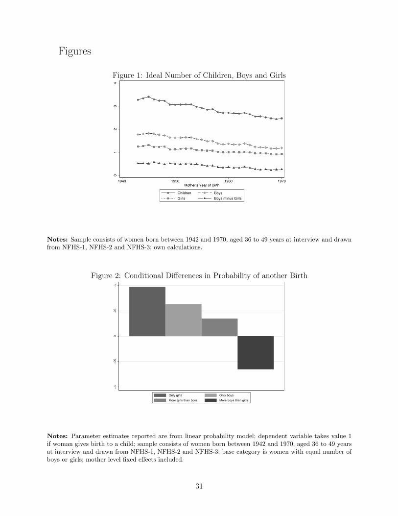
Figures

Figure 1: Ideal Number of Children, Boys and Girls

01

23

4

1940 1950 1960 1970Mother's Year of Birth

Children BoysGirls Boys minus Girls

Notes: Sample consists of women born between 1942 and 1970, aged 36 to 49 years at interview and drawnfrom NFHS-1, NFHS-2 and NFHS-3; own calculations.

Figure 2: Conditional Differences in Probability of another Birth

-.1

-.05

0.0

5.1

Only girls Only boys

More girls than boys More boys than girls

Notes: Parameter estimates reported are from linear probability model; dependent variable takes value 1if woman gives birth to a child; sample consists of women born between 1942 and 1970, aged 36 to 49 yearsat interview and drawn from NFHS-1, NFHS-2 and NFHS-3; base category is women with equal number ofboys or girls; mother level fixed effects included.

31

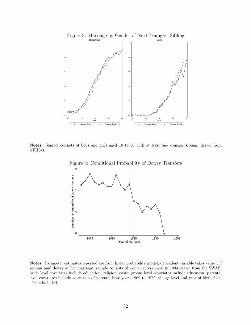
Figure 3: Marriage by Gender of Next Youngest Sibling

0.2

.4.6

.81

10 15 20 25 30Age

Younger Sister Younger Brother

Daughters

0.2

.4.6

.81

10 15 20 25 30Age

Younger Sister Younger Brother

Sons

Notes: Sample consists of boys and girls aged 10 to 30 with at least one younger sibling; drawn fromNFHS-3.

Figure 4: Conditional Probability of Dowry Transfers

-.6

-.4

-.2

0C

ondi

tiona

l Pro

babi

lity

of D

owry

Pay

men

t

1975 1980 1985 1990 1995Year of Marriage

Notes: Parameter estimates reported are from linear probability model; dependent variable takes value 1 ifwoman paid dowry at her marriage; sample consists of women interviewed in 1993 drawn from the SWAF;bride level covariates include education, religion, caste; groom level covariates include education; parentallevel covariates include education of parents; base years 1969 to 1972; village level and year of birth fixedeffects included.

32

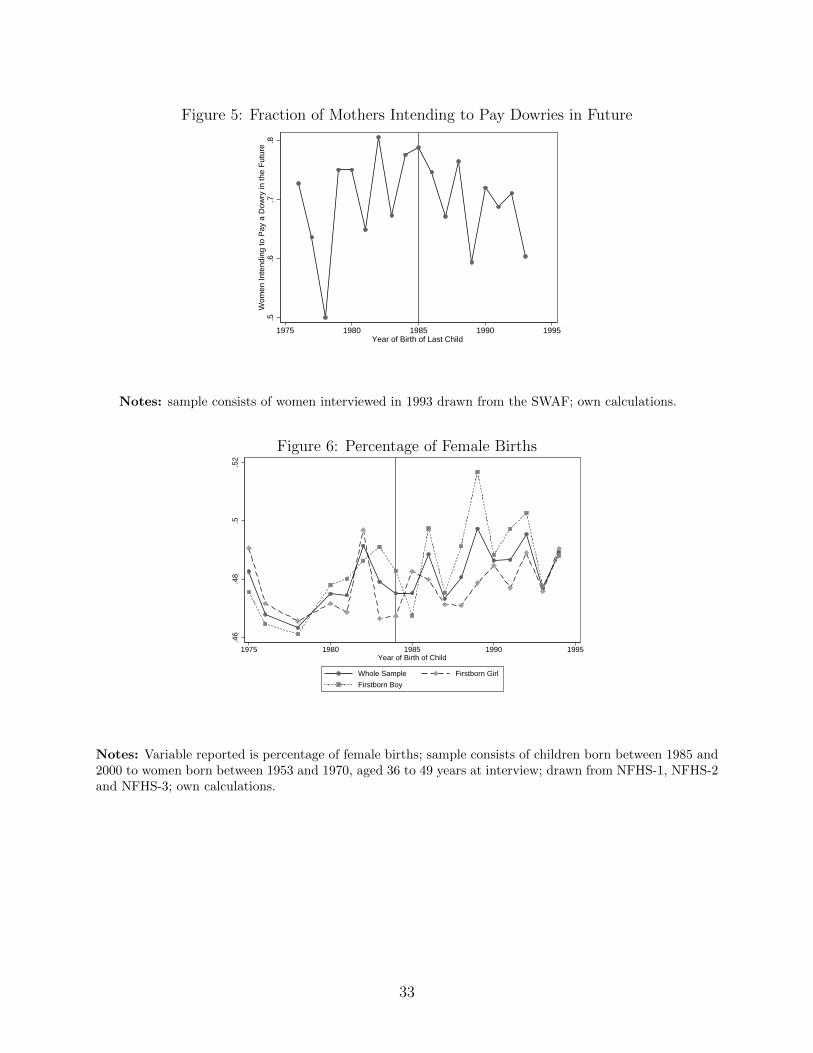
Figure 5: Fraction of Mothers Intending to Pay Dowries in Future

.5.6

.7.8

Wom

en In

tend

ing

to P

ay a

Dow

ry in

the

Fut

ure

1975 1980 1985 1990 1995Year of Birth of Last Child

Notes: sample consists of women interviewed in 1993 drawn from the SWAF; own calculations.

Figure 6: Percentage of Female Births

.46

.48

.5.5

2

1975 1980 1985 1990 1995Year of Birth of Child

Whole Sample Firstborn Girl

Firstborn Boy

Gender of Firstborn

Notes: Variable reported is percentage of female births; sample consists of children born between 1985 and2000 to women born between 1953 and 1970, aged 36 to 49 years at interview; drawn from NFHS-1, NFHS-2and NFHS-3; own calculations.

33

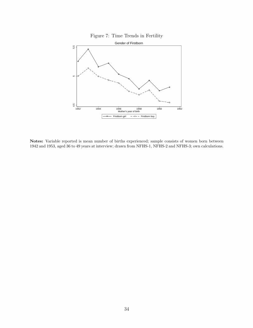
Figure 7: Time Trends in Fertility

4.5

55.

5

1942 1944 1946 1948 1950 1952Mother's year of birth

Firstborn girl Firstborn boy

Gender of Firstborn

Notes: Variable reported is mean number of births experienced; sample consists of women born between1942 and 1953, aged 36 to 49 years at interview; drawn from NFHS-1, NFHS-2 and NFHS-3; own calculations.

34

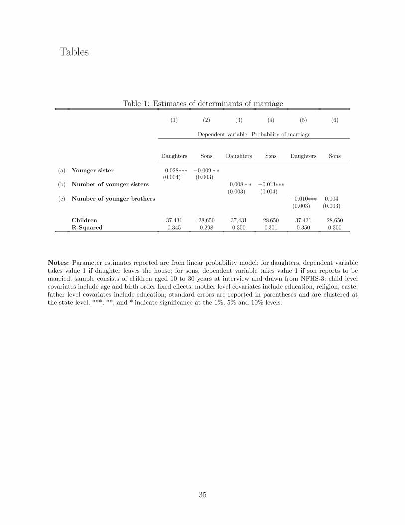
Tables

Table 1: Estimates of determinants of marriage

(1) (2) (3) (4) (5) (6)

Dependent variable: Probability of marriage

Daughters Sons Daughters Sons Daughters Sons

(a) Younger sister 0.028∗∗∗ −0.009 ∗ ∗(0.004) (0.003)

(b) Number of younger sisters 0.008 ∗ ∗ −0.013∗∗∗(0.003) (0.004)

(c) Number of younger brothers −0.010∗∗∗ 0.004(0.003) (0.003)

Children 37,431 28,650 37,431 28,650 37,431 28,650R-Squared 0.345 0.298 0.350 0.301 0.350 0.300

Notes: Parameter estimates reported are from linear probability model; for daughters, dependent variabletakes value 1 if daughter leaves the house; for sons, dependent variable takes value 1 if son reports to bemarried; sample consists of children aged 10 to 30 years at interview and drawn from NFHS-3; child levelcovariates include age and birth order fixed effects; mother level covariates include education, religion, caste;father level covariates include education; standard errors are reported in parentheses and are clustered atthe state level; ***, **, and * indicate significance at the 1%, 5% and 10% levels.

35

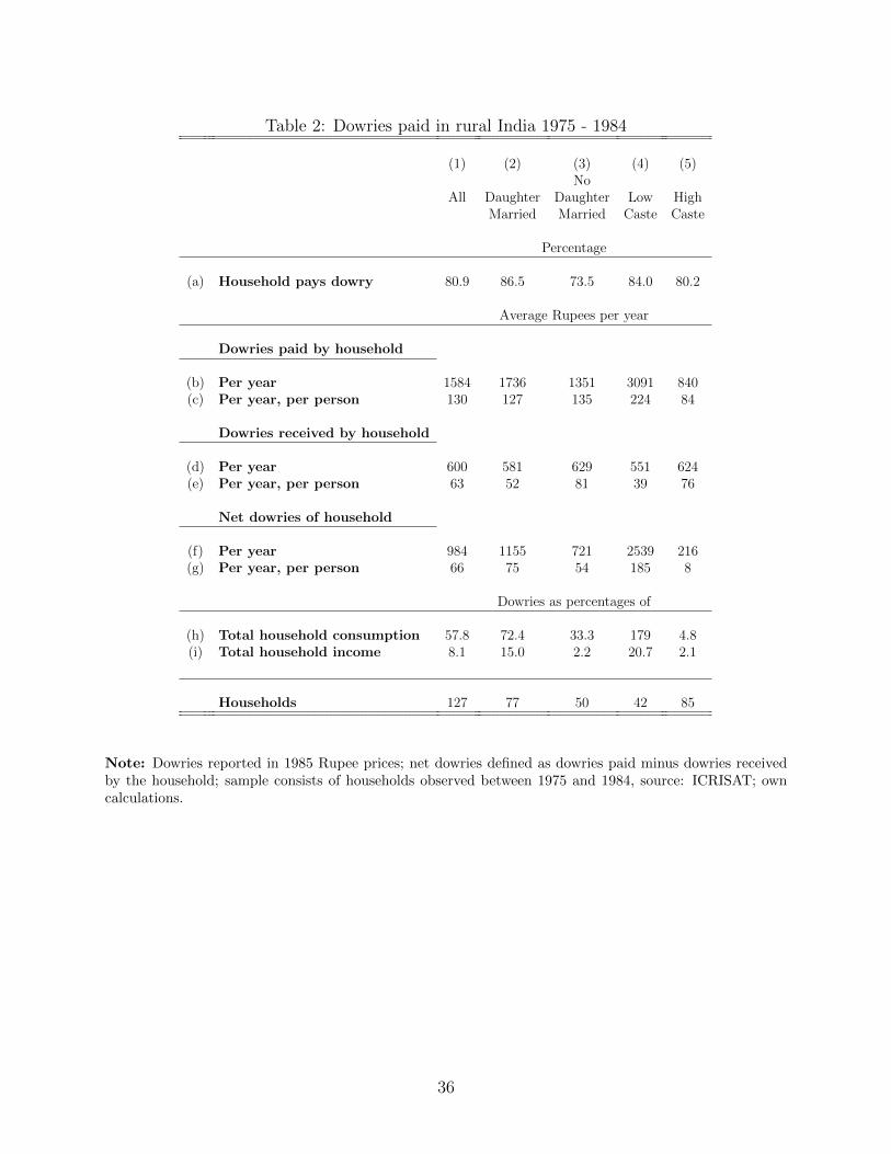
Table 2: Dowries paid in rural India 1975 - 1984

(1) (2) (3) (4) (5)No

All Daughter Daughter Low HighMarried Married Caste Caste

Percentage

(a) Household pays dowry 80.9 86.5 73.5 84.0 80.2

Average Rupees per year

Dowries paid by household

(b) Per year 1584 1736 1351 3091 840(c) Per year, per person 130 127 135 224 84

Dowries received by household

(d) Per year 600 581 629 551 624(e) Per year, per person 63 52 81 39 76

Net dowries of household

(f) Per year 984 1155 721 2539 216(g) Per year, per person 66 75 54 185 8

Dowries as percentages of

(h) Total household consumption 57.8 72.4 33.3 179 4.8(i) Total household income 8.1 15.0 2.2 20.7 2.1

Households 127 77 50 42 85

Note: Dowries reported in 1985 Rupee prices; net dowries defined as dowries paid minus dowries receivedby the household; sample consists of households observed between 1975 and 1984, source: ICRISAT; owncalculations.

36

Table 3: Estimates of Reduced Form Fertility Decision

(1) (2) (3) (4) (5)

Dependent variable: Probability of further birth

PredictedParameter estimates Probability

(a) Number of girls alive 0.018∗∗∗ 0.021∗∗∗ 0.011∗∗∗(0.004) (0.004) (0.004)

Birth order 1(b) Boy − 77%

(c) Girl 0.016∗∗∗ 78%(0.002)

Birth order 2(d) Boy, boy 0.018∗∗∗ 72%

(0.004)(e) Boy, girl 0.050∗∗∗ 75%

(0.003)(f) Girl, girl 0.130∗∗∗ 83%

(0.004)Birth order 3

(g) Boy, boy, boy −0.061∗∗∗ 64%(0.008)

(h) Boy, boy, girl −0.114∗∗∗ 58%(0.005)

(i) Boy, girl, girl 0.042∗∗∗ 74%(0.005)

(j) Girl, girl, girl 0.163∗∗∗ 86%(0.006)

Parental controls no yes no no noBirth order fixed effect yes yes yes yes yesMother fixed effect no no yes yes yesState fixed effect yes yes no no no

Observations 333,115 326,323 355,203 208,756 208,756Mothers 67,247 67,683 72,247 47,518 47,518R-Squared 0.250 0.265 0.387 0.320 0.320

Notes: Parameter estimates reported are from linear probability model; dependent variable takes value 1 ifwoman gives birth to a child; sample consists of women born between 1953 and 1970, aged 36 to 49 years atinterview and drawn from NFHS-1, NFHS-2 and NFHS-3; mother level covariates include education, religion,caste and birth cohort; father level covariates include education; standard errors are reported in parenthesesand are clustered at the state or mother level; ***, **, and * indicate significance at the 1%, 5% and 10%levels.

37

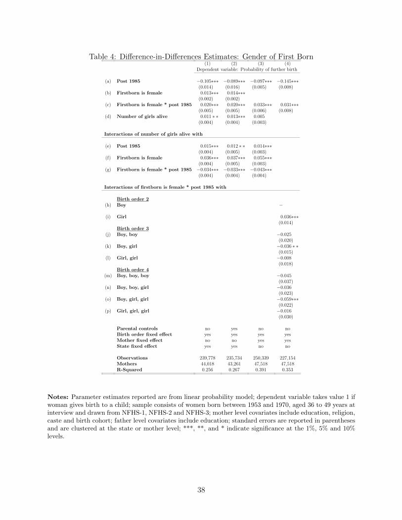
Table 4: Difference-in-Differences Estimates: Gender of First Born(1) (2) (3) (4)

Dependent variable: Probability of further birth

(a) Post 1985 −0.105∗∗∗ −0.089∗∗∗ −0.097∗∗∗ −0.145∗∗∗(0.014) (0.016) (0.005) (0.008)

(b) Firstborn is female 0.013∗∗∗ 0.014∗∗∗(0.002) (0.002)

(c) Firstborn is female * post 1985 0.020∗∗∗ 0.020∗∗∗ 0.033∗∗∗ 0.031∗∗∗(0.005) (0.005) (0.006) (0.008)

(d) Number of girls alive 0.011 ∗ ∗ 0.013∗∗∗ 0.005(0.004) (0.004) (0.003)

Interactions of number of girls alive with

(e) Post 1985 0.015∗∗∗ 0.012 ∗ ∗ 0.014∗∗∗(0.004) (0.005) (0.003)

(f) Firstborn is female 0.036∗∗∗ 0.037∗∗∗ 0.055∗∗∗(0.004) (0.005) (0.003)

(g) Firstborn is female * post 1985 −0.034∗∗∗ −0.033∗∗∗ −0.043∗∗∗(0.004) (0.004) (0.004)

Interactions of firstborn is female * post 1985 with

Birth order 2(h) Boy −

(i) Girl 0.036∗∗∗(0.014)

Birth order 3(j) Boy, boy −0.025

(0.020)(k) Boy, girl −0.036 ∗ ∗

(0.015)(l) Girl, girl −0.008

(0.018)Birth order 4

(m) Boy, boy, boy −0.045(0.037)

(n) Boy, boy, girl −0.036(0.023)

(o) Boy, girl, girl −0.059∗∗∗(0.022)

(p) Girl, girl, girl −0.016(0.030)

Parental controls no yes no noBirth order fixed effect yes yes yes yesMother fixed effect no no yes yesState fixed effect yes yes no no

Observations 239,778 235,734 250,339 227,154Mothers 44,018 43,261 47,518 47,518R-Squared 0.256 0.267 0.391 0.353

Notes: Parameter estimates reported are from linear probability model; dependent variable takes value 1 ifwoman gives birth to a child; sample consists of women born between 1953 and 1970, aged 36 to 49 years atinterview and drawn from NFHS-1, NFHS-2 and NFHS-3; mother level covariates include education, religion,caste and birth cohort; father level covariates include education; standard errors are reported in parenthesesand are clustered at the state or mother level; ***, **, and * indicate significance at the 1%, 5% and 10%levels.

38

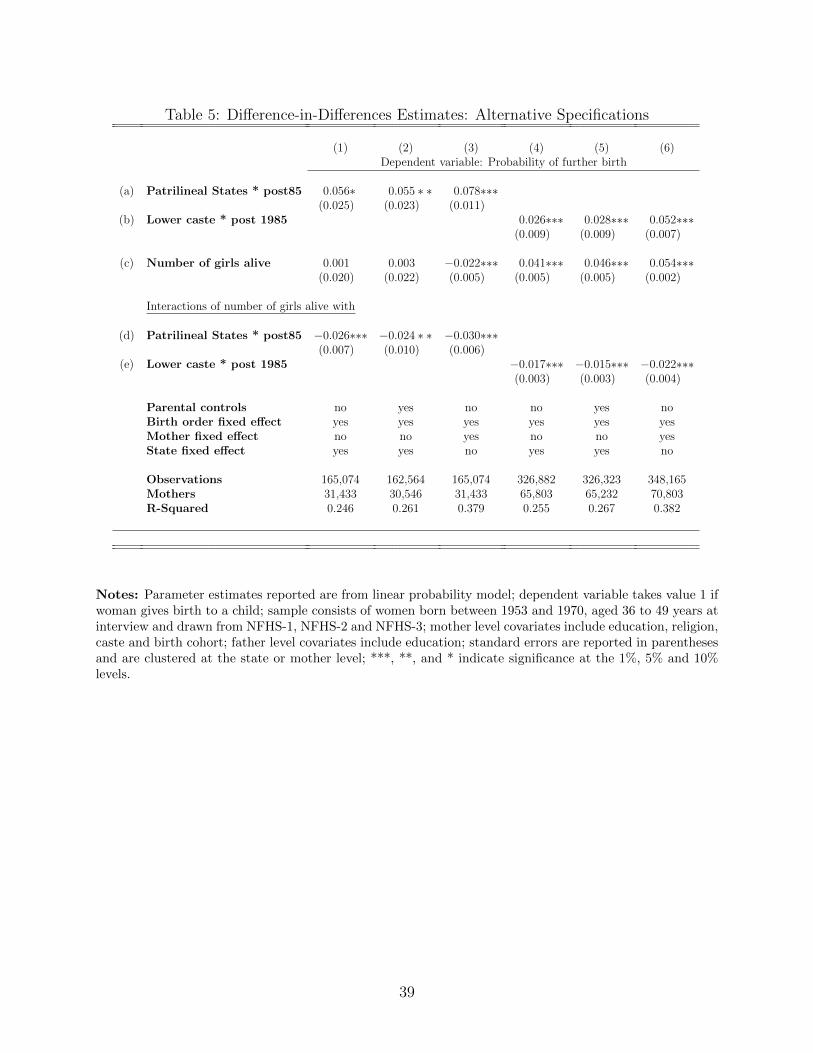
Table 5: Difference-in-Differences Estimates: Alternative Specifications

(1) (2) (3) (4) (5) (6)Dependent variable: Probability of further birth

(a) Patrilineal States * post85 0.056∗ 0.055 ∗ ∗ 0.078∗∗∗(0.025) (0.023) (0.011)

(b) Lower caste * post 1985 0.026∗∗∗ 0.028∗∗∗ 0.052∗∗∗(0.009) (0.009) (0.007)

(c) Number of girls alive 0.001 0.003 −0.022∗∗∗ 0.041∗∗∗ 0.046∗∗∗ 0.054∗∗∗(0.020) (0.022) (0.005) (0.005) (0.005) (0.002)

Interactions of number of girls alive with

(d) Patrilineal States * post85 −0.026∗∗∗ −0.024 ∗ ∗ −0.030∗∗∗(0.007) (0.010) (0.006)

(e) Lower caste * post 1985 −0.017∗∗∗ −0.015∗∗∗ −0.022∗∗∗(0.003) (0.003) (0.004)

Parental controls no yes no no yes noBirth order fixed effect yes yes yes yes yes yesMother fixed effect no no yes no no yesState fixed effect yes yes no yes yes no

Observations 165,074 162,564 165,074 326,882 326,323 348,165Mothers 31,433 30,546 31,433 65,803 65,232 70,803R-Squared 0.246 0.261 0.379 0.255 0.267 0.382

Notes: Parameter estimates reported are from linear probability model; dependent variable takes value 1 ifwoman gives birth to a child; sample consists of women born between 1953 and 1970, aged 36 to 49 years atinterview and drawn from NFHS-1, NFHS-2 and NFHS-3; mother level covariates include education, religion,caste and birth cohort; father level covariates include education; standard errors are reported in parenthesesand are clustered at the state or mother level; ***, **, and * indicate significance at the 1%, 5% and 10%levels.

39

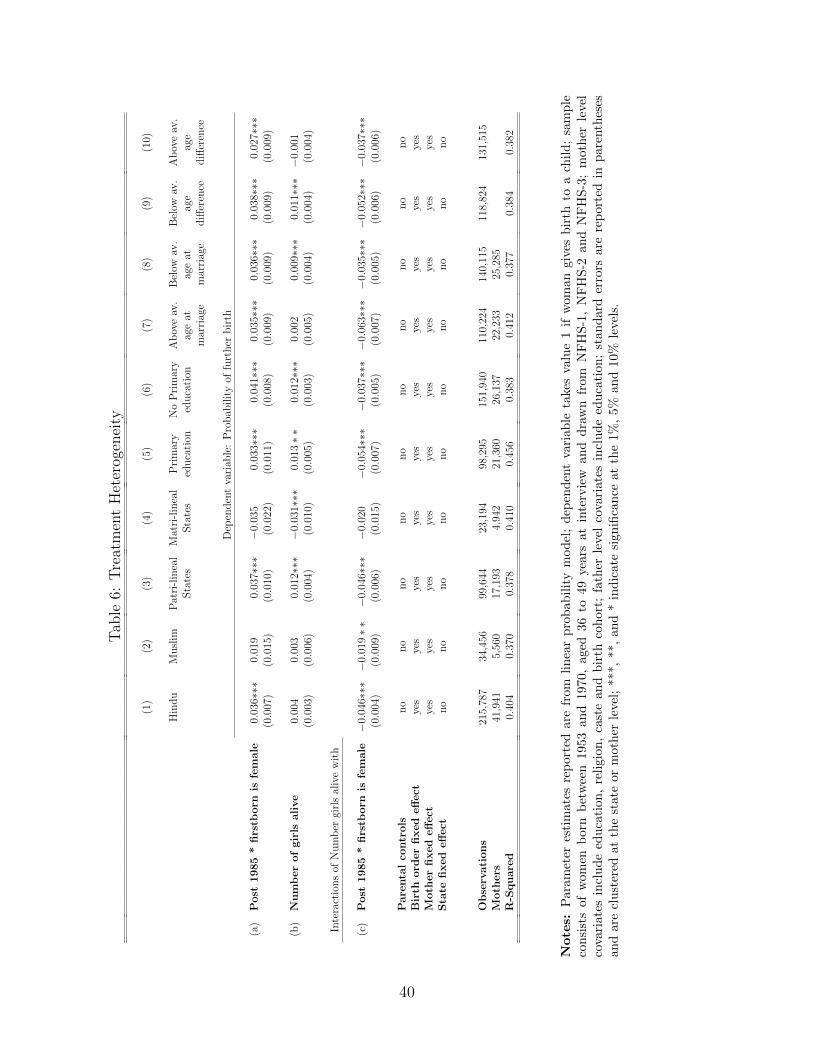
Tab

le6:

Tre

atm

ent

Het

erog

enei

ty

(1)

(2)

(3)

(4)

(5)

(6)

(7)

(8)

(9)

(10)

Hin

du

Musl

imP

atri

-lin

eal

Mat

ri-l

inea

lP

rim

ary

No

Pri

mar

yA

bov

eav

.B

elow

av.

Bel

owav

.A

bov

eav

.Sta

tes

Sta

tes

educa

tion

educa

tion

age

atag

eat

age

age

mar

riag

em

arri

age

diff

eren

cediff

eren

ce

Dep

enden

tva

riab

le:

Pro

bab

ilit

yof

furt

her

bir

th

(a)

Post

1985

*fi

rstb

orn

isfe

male

0.03

6∗∗∗

0.01

90.

037∗∗∗

−0.

035

0.03

3∗∗∗

0.04

1∗∗∗

0.03

5∗∗∗

0.03

6∗∗∗

0.03

8∗∗∗

0.02

7∗∗∗

(0.0

07)

(0.0

15)

(0.0

10)

(0.0

22)

(0.0

11)

(0.0

08)

(0.0

09)

(0.0

09)

(0.0

09)

(0.0

09)

(b)

Nu

mb

er

of

gir

lsali

ve

0.00

40.

003

0.01

2∗∗∗

−0.

031∗∗∗

0.01

3∗∗

0.01

2∗∗∗

0.00

20.

009∗∗∗

0.01

1∗∗∗−

0.00

1(0.0

03)

(0.0

06)

(0.0

04)

(0.0

10)

(0.0

05)

(0.0

03)

(0.0

05)

(0.0

04)

(0.0

04)

(0.0

04)

Inte

ract

ions

ofN

um

ber

girl

sal

ive

wit

h

(c)

Post

1985

*fi

rstb

orn

isfe

male−

0.04

6∗∗∗−

0.01

9∗∗−

0.04

6∗∗∗

−0.

020

−0.

054∗∗∗

−0.

037∗∗∗−

0.06

3∗∗∗−

0.03

5∗∗∗−

0.05

2∗∗∗−

0.03

7∗∗∗

(0.0

04)

(0.0

09)

(0.0

06)

(0.0

15)

(0.0

07)

(0.0

05)

(0.0

07)

(0.0

05)

(0.0

06)

(0.0

06)

Pare

nta

lco

ntr

ols

no

no

no

no

no

no

no

no

no

no

Bir

thord

er

fixed

eff

ect

yes

yes

yes

yes

yes

yes

yes

yes

yes

yes

Moth

er

fixed

eff

ect

yes

yes

yes

yes

yes

yes

yes

yes

yes

yes

Sta

tefi

xed

eff

ect

no

no

no

no

no

no

no

no

no

no

Ob

serv

ati

on

s21

5,78

734

,456

99,6

4423

,194

98,2

9515

1,94

011

0,22

414

0,11

511

8,82

413

1,51

5M

oth

ers

41,9

415,

560

17,1

934,

942

21,3

6026

,137

22,2

3325

,285

R-S

qu

are

d0.

404

0.37

00.

378

0.41

00.

456

0.38

30.

412

0.37

70.

384

0.38

2

Notes:

Par

amet

eres

tim

ates

rep

orte

dar

efr

omli

nea

rp

rob

ab

ilit

ym

od

el;

dep

end

ent

vari

ab

leta

kes

valu

e1

ifw

om

an

giv

esb

irth

toa

chil

d;

sam

ple

con

sist

sof

wom

enb

orn

bet

wee

n19

53an

d19

70,

aged

36

to49

years

at

inte

rvie

wan

dd

raw

nfr

om

NF

HS

-1,

NF

HS

-2an

dN

FH

S-3

;m

oth

erle

vel

cova

riat

esin

clu

de

edu

cati

on,

reli

gion

,ca

ste

and

bir

thco

hort

;fa

ther

leve

lco

vari

ate

sin

clu

de

edu

cati

on

;st

and

ard

erro

rsare

rep

ort

edin

pare

nth

eses

and

are

clu

ster

edat

the

stat

eor

mot

her

leve

l;***,

**,

an

d*

ind

icate

sign

ifica

nce

at

the

1%

,5%

an

d10%

leve

ls.

40

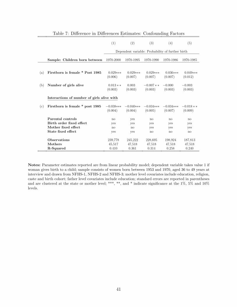
Table 7: Difference in Differences Estimates: Confounding Factors

(1) (2) (3) (4) (5)

Dependent variable: Probability of further birth

Sample: Children born between 1970-2000 1970-1995 1970-1990 1970-1986 1970-1985

(a) Firstborn is female * Post 1985 0.029∗∗∗ 0.029∗∗∗ 0.029∗∗∗ 0.036∗∗∗ 0.049∗∗∗(0.006) (0.007) (0.007) (0.007) (0.012)

(b) Number of girls alive 0.013 ∗ ∗ 0.003 −0.007 ∗ ∗ −0.000 −0.003(0.003) (0.003) (0.003) (0.003) (0.003)

Interactions of number of girls alive with

(c) Firstborn is female * post 1985 −0.038∗∗∗ −0.040∗∗∗ −0.034∗∗∗ −0.034∗∗∗ −0.018 ∗ ∗(0.004) (0.004) (0.005) (0.007) (0.009)

Parental controls no yes no no noBirth order fixed effect yes yes yes yes yesMother fixed effect no no yes yes yesState fixed effect yes yes no no no

Observations 239,778 245,222 228,695 198,924 187,813Mothers 45,517 47,518 47,518 47,518 47,518R-Squared 0.410 0.361 0.314 0.258 0.240

Notes: Parameter estimates reported are from linear probability model; dependent variable takes value 1 ifwoman gives birth to a child; sample consists of women born between 1953 and 1970, aged 36 to 49 years atinterview and drawn from NFHS-1, NFHS-2 and NFHS-3; mother level covariates include education, religion,caste and birth cohort; father level covariates include education; standard errors are reported in parenthesesand are clustered at the state or mother level; ***, **, and * indicate significance at the 1%, 5% and 10%levels.

41

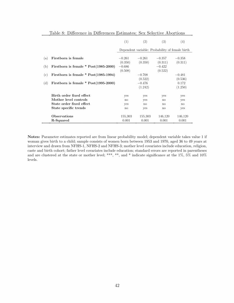
Table 8: Difference in Differences Estimates: Sex Selective Abortions

(1) (2) (3) (4)

Dependent variable: Probability of female birth

(a) Firstborn is female −0.261 −0.261 −0.357 −0.358(0.350) (0.350) (0.311) (0.311)

(b) Firstborn is female * Post(1985-2000) −0.686 −0.422(0.508) (0.522)

(c) Firstborn is female * Post(1985-1994) −0.708 −0.481(0.522) (0.536)

(d) Firstborn is female * Post(1995-2000) −0.476 0.172(1.242) (1.250)

Birth order fixed effect yes yes yes yesMother level controls no yes no yesState order fixed effect yes no no noState specific trends no yes no yes

Observations 155,303 155,303 146,120 146,120R-Squared 0.001 0.001 0.001 0.001

Notes: Parameter estimates reported are from linear probability model; dependent variable takes value 1 ifwoman gives birth to a child; sample consists of women born between 1953 and 1970, aged 36 to 49 years atinterview and drawn from NFHS-1, NFHS-2 and NFHS-3; mother level covariates include education, religion,caste and birth cohort; father level covariates include education; standard errors are reported in parenthesesand are clustered at the state or mother level; ***, **, and * indicate significance at the 1%, 5% and 10%levels.

42

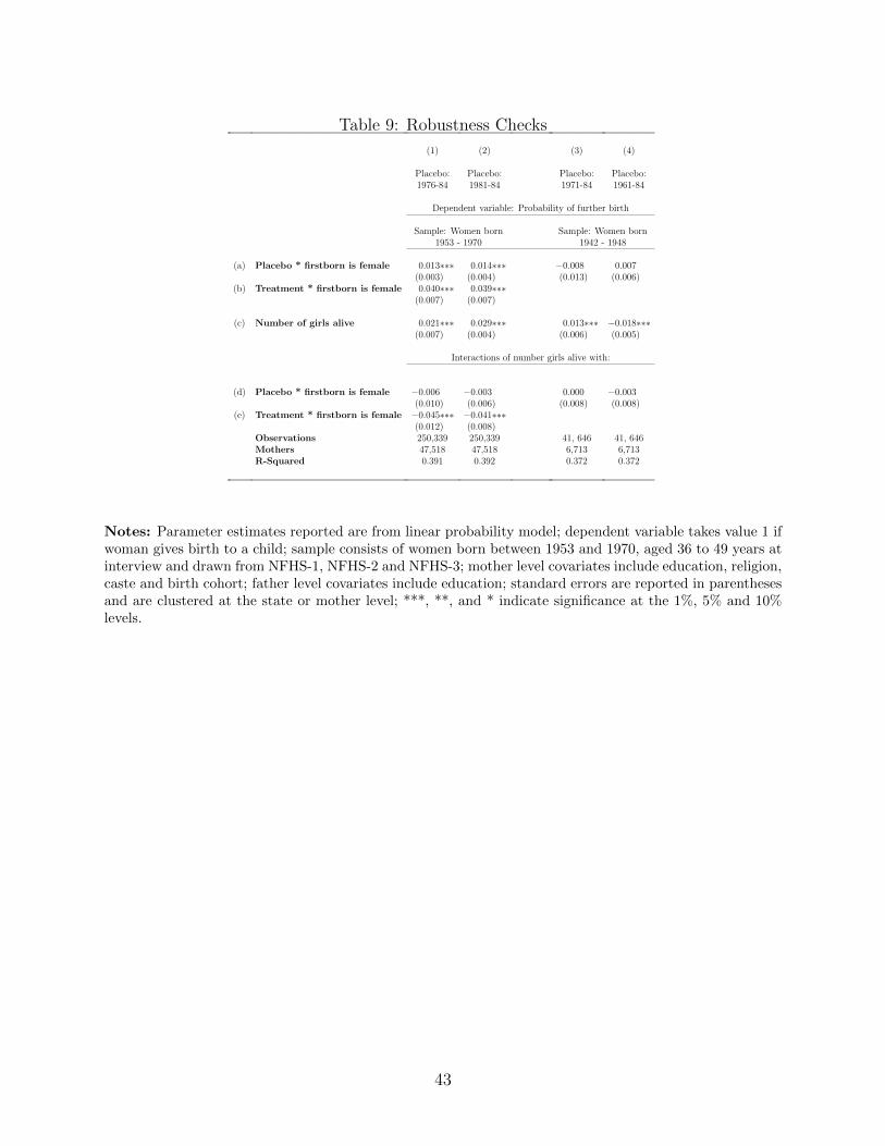
Table 9: Robustness Checks

(1) (2) (3) (4)

Placebo: Placebo: Placebo: Placebo:1976-84 1981-84 1971-84 1961-84

Dependent variable: Probability of further birth

Sample: Women born Sample: Women born1953 - 1970 1942 - 1948

(a) Placebo * firstborn is female 0.013∗∗∗ 0.014∗∗∗ −0.008 0.007(0.003) (0.004) (0.013) (0.006)

(b) Treatment * firstborn is female 0.040∗∗∗ 0.039∗∗∗(0.007) (0.007)

(c) Number of girls alive 0.021∗∗∗ 0.029∗∗∗ 0.013∗∗∗ −0.018∗∗∗(0.007) (0.004) (0.006) (0.005)

Interactions of number girls alive with:

(d) Placebo * firstborn is female −0.006 −0.003 0.000 −0.003(0.010) (0.006) (0.008) (0.008)

(e) Treatment * firstborn is female −0.045∗∗∗ −0.041∗∗∗(0.012) (0.008)

Observations 250,339 250,339 41, 646 41, 646Mothers 47,518 47,518 6,713 6,713R-Squared 0.391 0.392 0.372 0.372

Notes: Parameter estimates reported are from linear probability model; dependent variable takes value 1 ifwoman gives birth to a child; sample consists of women born between 1953 and 1970, aged 36 to 49 years atinterview and drawn from NFHS-1, NFHS-2 and NFHS-3; mother level covariates include education, religion,caste and birth cohort; father level covariates include education; standard errors are reported in parenthesesand are clustered at the state or mother level; ***, **, and * indicate significance at the 1%, 5% and 10%levels.

43

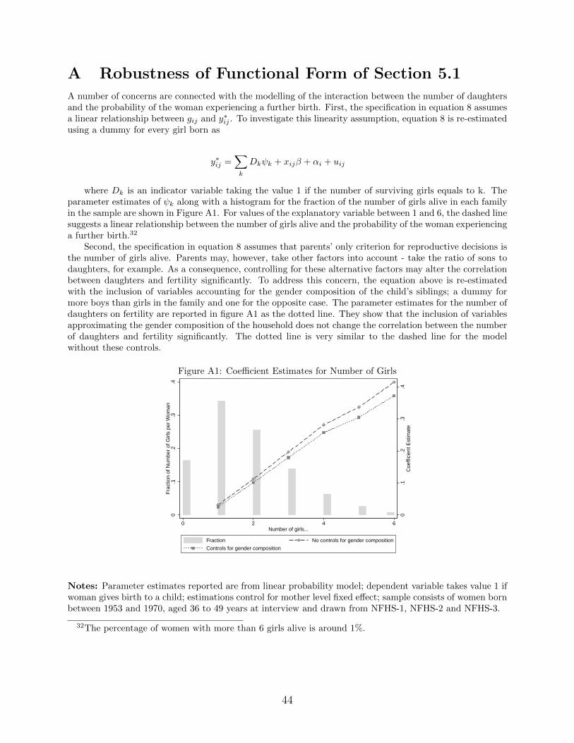
A Robustness of Functional Form of Section 5.1

A number of concerns are connected with the modelling of the interaction between the number of daughtersand the probability of the woman experiencing a further birth. First, the specification in equation 8 assumesa linear relationship between gij and y∗ij . To investigate this linearity assumption, equation 8 is re-estimatedusing a dummy for every girl born as

y∗ij =∑k

Dkψk + xijβ + αi + uij

where Dk is an indicator variable taking the value 1 if the number of surviving girls equals to k. Theparameter estimates of ψk along with a histogram for the fraction of the number of girls alive in each familyin the sample are shown in Figure A1. For values of the explanatory variable between 1 and 6, the dashed linesuggests a linear relationship between the number of girls alive and the probability of the woman experiencinga further birth.32

Second, the specification in equation 8 assumes that parents’ only criterion for reproductive decisions isthe number of girls alive. Parents may, however, take other factors into account - take the ratio of sons todaughters, for example. As a consequence, controlling for these alternative factors may alter the correlationbetween daughters and fertility significantly. To address this concern, the equation above is re-estimatedwith the inclusion of variables accounting for the gender composition of the child’s siblings; a dummy formore boys than girls in the family and one for the opposite case. The parameter estimates for the number ofdaughters on fertility are reported in figure A1 as the dotted line. They show that the inclusion of variablesapproximating the gender composition of the household does not change the correlation between the numberof daughters and fertility significantly. The dotted line is very similar to the dashed line for the modelwithout these controls.

Figure A1: Coefficient Estimates for Number of Girls

0.1

.2.3

.4C

oeffi

cien

t Est

imat

e

0.1

.2.3

.4F

ract

ion

of N

umbe

r of

Girl

s pe

r W

oman

0 2 4 6Number of girls...

Fraction No controls for gender composition

Controls for gender composition

Notes: Parameter estimates reported are from linear probability model; dependent variable takes value 1 ifwoman gives birth to a child; estimations control for mother level fixed effect; sample consists of women bornbetween 1953 and 1970, aged 36 to 49 years at interview and drawn from NFHS-1, NFHS-2 and NFHS-3.

32The percentage of women with more than 6 girls alive is around 1%.

44

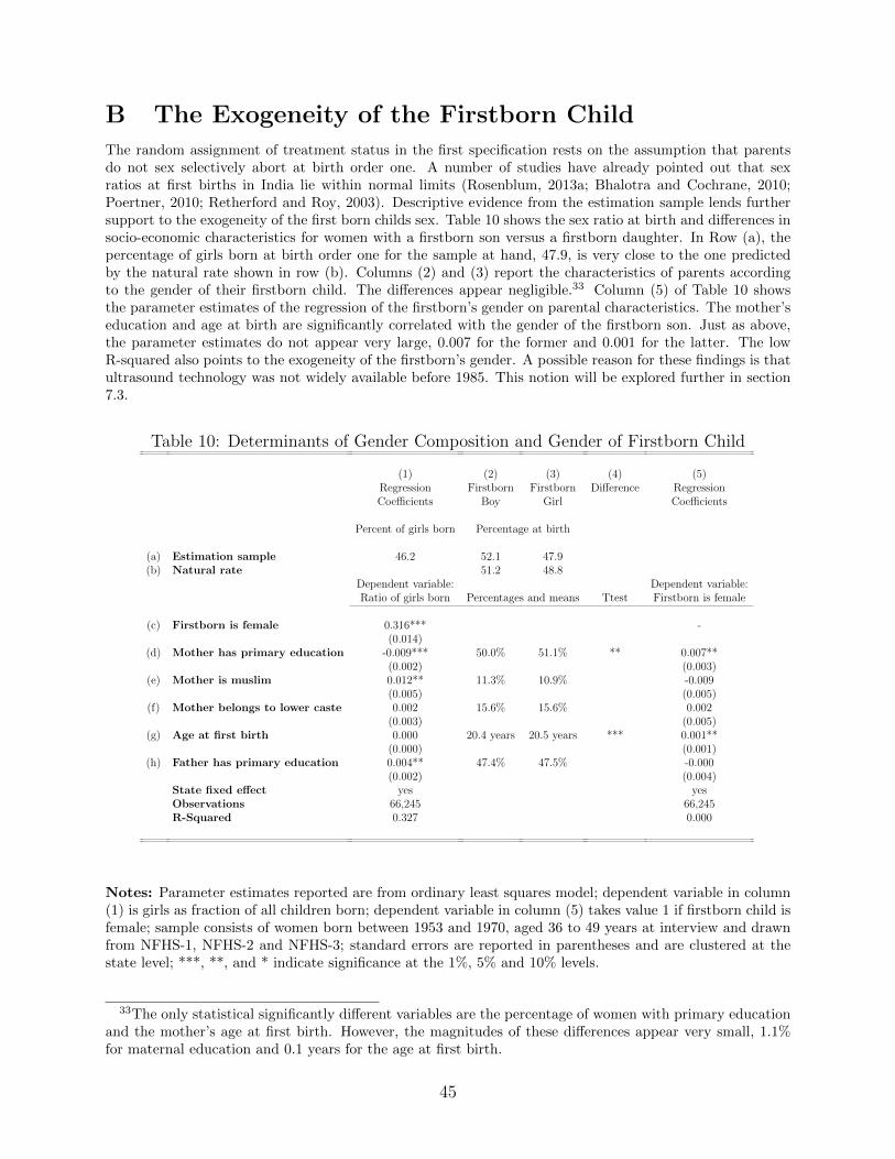
B The Exogeneity of the Firstborn Child

The random assignment of treatment status in the first specification rests on the assumption that parentsdo not sex selectively abort at birth order one. A number of studies have already pointed out that sexratios at first births in India lie within normal limits (Rosenblum, 2013a; Bhalotra and Cochrane, 2010;Poertner, 2010; Retherford and Roy, 2003). Descriptive evidence from the estimation sample lends furthersupport to the exogeneity of the first born childs sex. Table 10 shows the sex ratio at birth and differences insocio-economic characteristics for women with a firstborn son versus a firstborn daughter. In Row (a), thepercentage of girls born at birth order one for the sample at hand, 47.9, is very close to the one predictedby the natural rate shown in row (b). Columns (2) and (3) report the characteristics of parents accordingto the gender of their firstborn child. The differences appear negligible.33 Column (5) of Table 10 showsthe parameter estimates of the regression of the firstborn’s gender on parental characteristics. The mother’seducation and age at birth are significantly correlated with the gender of the firstborn son. Just as above,the parameter estimates do not appear very large, 0.007 for the former and 0.001 for the latter. The lowR-squared also points to the exogeneity of the firstborn’s gender. A possible reason for these findings is thatultrasound technology was not widely available before 1985. This notion will be explored further in section7.3.

Table 10: Determinants of Gender Composition and Gender of Firstborn Child

(1) (2) (3) (4) (5)Regression Firstborn Firstborn Difference RegressionCoefficients Boy Girl Coefficients

Percent of girls born Percentage at birth

(a) Estimation sample 46.2 52.1 47.9(b) Natural rate 51.2 48.8

Dependent variable: Dependent variable:Ratio of girls born Percentages and means Ttest Firstborn is female

(c) Firstborn is female 0.316*** -(0.014)

(d) Mother has primary education -0.009*** 50.0% 51.1% ** 0.007**(0.002) (0.003)

(e) Mother is muslim 0.012** 11.3% 10.9% -0.009(0.005) (0.005)

(f) Mother belongs to lower caste 0.002 15.6% 15.6% 0.002(0.003) (0.005)

(g) Age at first birth 0.000 20.4 years 20.5 years *** 0.001**(0.000) (0.001)

(h) Father has primary education 0.004** 47.4% 47.5% -0.000(0.002) (0.004)

State fixed effect yes yesObservations 66,245 66,245R-Squared 0.327 0.000

Notes: Parameter estimates reported are from ordinary least squares model; dependent variable in column(1) is girls as fraction of all children born; dependent variable in column (5) takes value 1 if firstborn child isfemale; sample consists of women born between 1953 and 1970, aged 36 to 49 years at interview and drawnfrom NFHS-1, NFHS-2 and NFHS-3; standard errors are reported in parentheses and are clustered at thestate level; ***, **, and * indicate significance at the 1%, 5% and 10% levels.

33The only statistical significantly different variables are the percentage of women with primary educationand the mother’s age at first birth. However, the magnitudes of these differences appear very small, 1.1%for maternal education and 0.1 years for the age at first birth.

45