Daughters, Dowries, Deliveries: The E↵ect of

Marital Payments on Fertility Choices in India

Marco Alfano⇤

Department of Economics

University College London

October 2013

Abstract

This study estimates the e↵ect of dowries on fertility in India. The future dowryassociated with the birth of each child introduces a gender-specific cost to itsparents. This leads families with more daughters to have higher fertility. Foridentification, the paper exploits a revision in anti-dowry law in combinationwith pre-treatment heterogeneity across the gender of the first child, maternalethnicity and birth cohort. The resulting decrease in expected dowries attenuatesthe correlation between daughters and their parents’ birth rates. The e↵ect isstrongest for lower birth orders and for more educated and autonomous women.

JEL Classifications: O15, J12, J13

Keywords: Dowry, Fertility, India, Son Preferences

⇤Department of Economics, University College London, Gower Street, WC1E 6BT, London; tel:+44 20 3549 5352; email: m.alfano@ucl.ac.uk. For helpful comments, I would like to thank WijiArulampalam, Konrad Burchardi, Thomas Cornelissen, Christian Dustmann, Luigi Minale, RobinNaylor, Anna Okatenko, Sarmistha Pal, Imran Rasul, Uta Schonberg, Jeremy Smith, Jan Stuhler andseminar participants at the Centre for Research of Analysis and Migration, Institute for InternationalEconomic Studies and National Institute for Social and Economic Research. I gratefully acknowledgefinancial support from the British Academy and the Norface Research Programme on Migration. Allerrors are my own.

1

1 Introduction

It is widely accepted that Indian fertility is key to world demography. Over the past 5

years, the number of children born in India has accounted for about one fifth of global

births (UN, 2013).1 Moreover, the country’s fertility rates are likely to translate into

future population growth; India is estimated to overtake China as the world’s most

populous country within the next 20 years.2 Concerns that these phenomena will lead

to a scarcity of resources and societal problems (UNDP, 2006) have sparked an increased

interest in the determinants of fertility choices. For each individual household, parents’

desire to achieve a determined gender composition of their children has been identified

as an important factor influencing reproductive decisions (Angrist and Evans, 1998;

for instance).

A growing body of evidence points to parents favouring male o↵spring (Dahl and

Moretti, 2008; among others). South East Asia in general and India in particular,

have been argued to exhibit especially strong preferences for sons, based on the belief

that sons are more valuable than daughters (Pande and Astone, 2007; Das Gupta

et al., 2003; Clark, 2000). The presence of significant gender gaps in a number of

human development indicators such as mortality (Bhargava, 2003; Arnold et al., 2002),

nutrition (Jayachandran and Kuziemko, 2011; Oster, 2009; Pande, 2003), abortions

(Bhalotra and Cochrane, 2010) and more recently child care (Barcellos et al., 2012)

further corroborates these findings. Indeed, various studies have argued that parents

adjust their reproductive behaviour in an e↵ort to achieve their ideal mix of sons

and daughters (Arokiasamy, 2002; Yount et al., 2000; Srinivasan, 1992). Empirically,

this behaviour results in a correlation between the gender composition of a couple’s

o↵spring and its fertility rates; ceteris paribus, the presence of daughters in the family

tends to increase fertility, whereas sons decrease birth rates. This correlation is often

been interpreted as ”son preference” in fertility behaviour. Yamaguchi (1989) and

Dreze and Murthi (1999) argue that this behaviour substantially increases fertility

rates. Jensen (2003) meanwhile points out that these patterns ultimately decrease

young girls’ welfare by concentrating daughters into larger families. Whilst it is well

documented that parents condition reproductive choices on the gender composition of

their o↵spring, our understanding of the underlying mechanisms behind this behaviour

1129 million births for India and 675 million births for the world2Figures come from the Population Reference Bureau: http://www.prb.org/. The 2025 and 2050

estimates for India are 1.444 billion and 1.747 billion individuals. For China 1.476 billion and 1.437billion individuals.

2

remains rudimentary. In particular, we are yet to identify the role pecuniary factors

play in determining these patterns.

The present study addresses this gap by investigating the extent to which the

correlation between the gender composition of a couple’s o↵spring and its fertility

choices is the result of gender specific economic costs of children. The focus is on one

custom that is particularly widespread in India: dowries, defined as marital transfers of

resources from the family of the bride to the groom or his family (see Anderson, 2007a;

for a review). The prospect of these marital payments introduces an expected future

cost that is conditional on the gender of each child: the birth of a girl will be associated

with a negative, and the birth of a boy with a positive, income shock at the time of

his or her marriage. Forward-looking parents are likely to take this into account when

making reproductive decisions. Indeed, qualitative evidence has suggested a strong

correlation between dowries and reproductive decisions (Diamond-Smith et al., 2008).

In contrast to other expenses related to children, where the gender specific component

can be hard to determine - take educational expenses for example - the focus on dowries

will allow us to better approximate the e↵ect of boy’s or a girl’s birth on the finances

of a family.

The theoretical framework views the total number of a couple’s o↵spring as the

result of a series of sequential yes/no decisions. After every birth, parents decide

whether or not to opt for a further child. Individuals are assumed to have children for

two reasons. First, to increase their utility net of costs; second, to influence the flow of

costs and returns associated with their children. The latter mechanism stipulates that

parents aim to o↵set the negative income shock associated with the birth of a daughter

with the revenue generated from dowries received at the time of a son’s marriage.

As a consequence, couples’, whose o↵spring are mainly female, are likely to continue

childbearing beyond their ideal family size. In contrast to fertility models rooted in the

standard constrained optimisation setting, where parents decide on the optimal number

of children at the outset of their reproductive years (see Becker and Lewis, 1973; for

instance), this way of viewing fertility allows parents to revise their reproductive choices

as the gender of each child is revealed birth by birth. The model has the following

implications: (i) there exists a negative correlation between the expected value of the

dowry and the probability of the woman experiencing a further birth; (ii) conditional

on the total number of children, there exists a positive correlation between the number

of daughters and the probability of the couple opting for a further birth; and (iii) the

3

correlation mentioned in point (ii) depends positively on the expected value of the

dowry.

To test the three aforementioned implications empirically, this study estimates a

reduced form sequential fertility model using information on completed birth histories

from three rounds of the National Family Health Survey (NFHS, 1994; 1999; 2007b). At

every birth order, the parameter estimates show a strong positive correlation between

the number of daughters in the family and the probability of the woman experiencing a

further birth. This lends empirical support to theoretical implication (ii). On average

the birth of a girl increases the conditional probability of a woman experiencing a

further birth by 7 percentage points. The correlation, further, appears to be the

strongest between the second and fourth birth.

To isolate the causal e↵ect of dowries on fertility choices, the present analysis ex-

ploits a substantial revision in India’s anti-dowry laws. The ine↵ective and widely

criticised Dowry Prohibition Act of 1961 was tightened in 1985 under the Dowry Pro-

hibition Rules. The changes encompassed more stringent monitoring of transfers asso-

ciated with marriage as well as substantial increases in penalties for o↵enders. Evidence

from the Survey of Status of Women and Fertility (SWAF, 2000) shows a marked de-

crease in the conditional probability of dowry payments in the years immediately after

the introduction of the policy, which, in turn, is likely to decrease parents’ expectation

that a dowry will be transferred upon their children’s marriage. This is borne out by

descriptive evidence from the SWAF, which suggests that mothers became less willing

to pay a dowry for children born after the implementation of the policy. With regard

to fertility decisions, the theoretical model predicts that this shift in expectations will

cause an increase in the probability of the couple opting for a further birth - see im-

plication (i) - as well as an attenuation of the positive correlation between the number

of daughters and birth rates - see implication (iii).

The policy change is evaluated in a di↵erence in di↵erences framework, which allows

for a change in the intercept as well as in the slope parameter. Because the Dowry

Prohibition Rules were introduced simultaneously in the whole of India in 1985, this

paper exploits the heterogeneity in dowry payments before that year to identify the

e↵ect of the policy on reproductive decisions. It argues that the impact of the policy on

an individual family was proportional to the average dowry paid and received by that

household in the pre-treatment period. In other words, the change in the law had an

especially strong e↵ect on couples paying particularly high dowries before 1985. The

4

specification defines treatment status along the lines of the gender of the firstborn child

and employs mothers, whose firstborn is female, as treated individuals. The woman’s

ethnicity is employed as a further way to distinguish the treatment and control group.

Evidence on dowry transfers between 1975 and 1984 from the International Crops

Research Institute for the Semi-Arid Tropics (ICRISAT, 1984) suggests that these two

groups paid significantly higher dowries than average. To strengthen the specification

further, the empirical model takes advantage of the fact that some women had come

to the end of their reproductive years by the time the changes in the policy had been

implemented.

The estimates suggest that the amendment of the law impacted upon fertility be-

haviour significantly. The policy change is estimated to have lead to an one-o↵ increase

the probability of a woman experiencing a further birth of 4 percentage points; this is

in line with prediction (i). The specification further points to an attenuation in the

previously observed correlation between the number of girls in the household and fer-

tility rate of 5 percentage points, this lends support to prediction (iii). For the treated,

the policy decreased the influence of the gender composition on fertility by 20 percent.

The e↵ect appears particularly strong for children of lower birth orders and for more

educated and autonomous women.

By analysing the link between dowries and fertility decisions, this study attempts

to shed light on as yet unanswered questions such as: why is son preference still

so widespread? What are its determinants? And how does it influence fertility de-

cisions? Insights into these issues can uncover some of the mechanisms underlying

fertility choices and are thus likely to be of interest to policy makers concerned with,

for instance, fertility rates or son preferring behaviour more generally. Moreover, the

present analysis aims to add to the growing knowledge base on dowries. Whilst the

determinants of marital payments (Botticini and Siow, 2003; for instance) as well as

their e↵ects on brides (Bloch and Rao, 2002) have received growing attention, little is

known on the ramifications of this practice on other household members.

The remainder of the paper is structured as follows: Section 2 introduces the data

and gives motivating descriptive evidence. Section 3 explains the practice of dowries

and the legal framework. Section 4 lays out a theoretical framework to help concep-

tualise the e↵ect changes in dowry policies can have on fertility choices. Section 5

analyses the influence of a couple’s gender composition on fertility; the e↵ect of the

policy change on this behaviour is explored in section 6. Section 7 shows the results

5

of the empirical analysis, the robustness of which is shown in section 8. Section 9

concludes.

2 Fertility and Gender Preferences in India

This study starts from the qualitative observation that, when asked about their ideal

number of children, women in India tend to report a preference for sons over daughters.3

2.1 The Data

The present analysis employs data drawn from three rounds of the National Family

Health Survey (NFHS) for India (NFHS-1, NFHS-2 and NFHS-3), a nationally rep-

resentative survey of Indian households. The NFHS is part of the Demographic and

Health Surveys series, which is conducted in about 70 low and middle income countries

around the world.4 The questionnaires collect extensive information on health, nutri-

tion, population and focus particular on women and children. The NFHS-1 (Interna-

tional Institute for Population Sciences and Macro International, 1994) was carried out

in 1992 and 1993 and interviewed 89,777 ever-married women aged 13 to 49; the NFHS-

2 (International Institute for Population Sciences and Macro International, 1999) was

conducted in 1998 and 1999 and interviewed 89,199 ever married women aged 15 to 49;

finally the NFHS-3 (International Institute for Population Sciences and Macro Inter-

national, 2007b) was implemented in 2005 and 2006 and interviewed 124,385 women

aged 15 to 49. Each round collected detailed information on women’s complete birth

histories including the number, gender and morality status of all births.

Individuals selected for the present purpose are women, who have experienced at

least one birth and who have come to the end of their reproductive years, i.e. aged 36

or above. Although biologically women can still conceive in their late 30s and early

40s, the percentage of women doing so in India is very low. The NFHS-3 final report

(NFHS, 2007a) indicates that fertility at ages 35 and above accounts for only 4 percent

of total fertility in urban and 7 percent in rural areas.5 Similarly, the omission of

childless women is unlikely to bias the results significantly, only 3.6 percent of women

3The estimates reported are for women aged 35 or above at the time of interview. The samepatterns, however, can be found in younger women.

4The data are publicly available at measuredhs.com5Restricting the sample to women aged 40 and above does not alter the results significantly.

6

aged 35 to 40 in India have never experienced a birth (NFHS-3, 2007a). The final

sample consists of 412,378 children of 99,533 mothers born between the years 1942 and

1970.

2.2 Descriptive Statistics

Women in the estimation sample show relatively low levels of education, around half of

the individuals have completed primary school. The majority are Hindu (85 percent)

with a minority of Muslim women (11 percent). Around 15 percent belong to a sched-

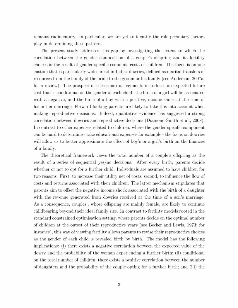
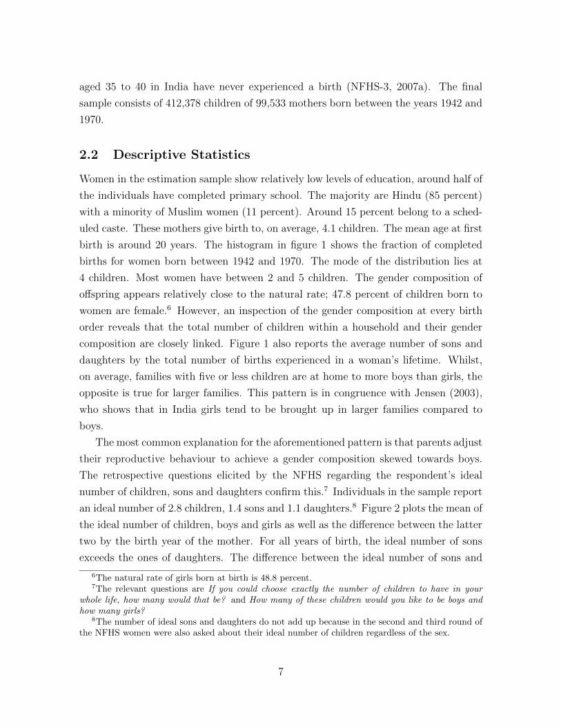
uled caste. These mothers give birth to, on average, 4.1 children. The mean age at first

birth is around 20 years. The histogram in figure 1 shows the fraction of completed

births for women born between 1942 and 1970. The mode of the distribution lies at

4 children. Most women have between 2 and 5 children. The gender composition of

o↵spring appears relatively close to the natural rate; 47.8 percent of children born to

women are female.6 However, an inspection of the gender composition at every birth

order reveals that the total number of children within a household and their gender

composition are closely linked. Figure 1 also reports the average number of sons and

daughters by the total number of births experienced in a woman’s lifetime. Whilst,

on average, families with five or less children are at home to more boys than girls, the

opposite is true for larger families. This pattern is in congruence with Jensen (2003),

who shows that in India girls tend to be brought up in larger families compared to

boys.

The most common explanation for the aforementioned pattern is that parents adjust

their reproductive behaviour to achieve a gender composition skewed towards boys.

The retrospective questions elicited by the NFHS regarding the respondent’s ideal

number of children, sons and daughters confirm this.7 Individuals in the sample report

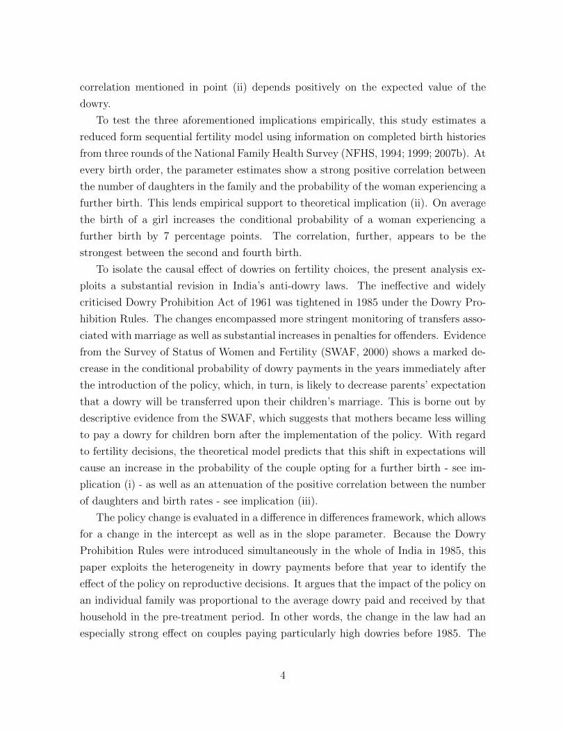
an ideal number of 2.8 children, 1.4 sons and 1.1 daughters.8 Figure 2 plots the mean of

the ideal number of children, boys and girls as well as the di↵erence between the latter

two by the birth year of the mother. For all years of birth, the ideal number of sons

exceeds the ones of daughters. The di↵erence between the ideal number of sons and

6The natural rate of girls born at birth is 48.8 percent.7The relevant questions are If you could choose exactly the number of children to have in your

whole life, how many would that be? and How many of these children would you like to be boys andhow many girls?

8The number of ideal sons and daughters do not add up because in the second and third round ofthe NFHS women were also asked about their ideal number of children regardless of the sex.

7

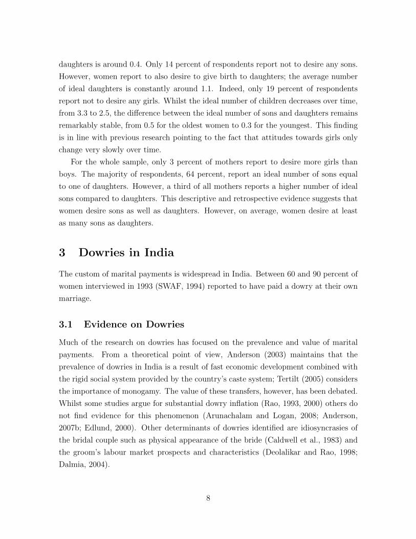
daughters is around 0.4. Only 14 percent of respondents report not to desire any sons.

However, women report to also desire to give birth to daughters; the average number

of ideal daughters is constantly around 1.1. Indeed, only 19 percent of respondents

report not to desire any girls. Whilst the ideal number of children decreases over time,

from 3.3 to 2.5, the di↵erence between the ideal number of sons and daughters remains

remarkably stable, from 0.5 for the oldest women to 0.3 for the youngest. This finding

is in line with previous research pointing to the fact that attitudes towards girls only

change very slowly over time.

For the whole sample, only 3 percent of mothers report to desire more girls than

boys. The majority of respondents, 64 percent, report an ideal number of sons equal

to one of daughters. However, a third of all mothers reports a higher number of ideal

sons compared to daughters. This descriptive and retrospective evidence suggests that

women desire sons as well as daughters. However, on average, women desire at least

as many sons as daughters.

3 Dowries in India

The custom of marital payments is widespread in India. Between 60 and 90 percent of

women interviewed in 1993 (SWAF, 1994) reported to have paid a dowry at their own

marriage.

3.1 Evidence on Dowries

Much of the research on dowries has focused on the prevalence and value of marital

payments. From a theoretical point of view, Anderson (2003) maintains that the

prevalence of dowries in India is a result of fast economic development combined with

the rigid social system provided by the country’s caste system; Tertilt (2005) considers

the importance of monogamy. The value of these transfers, however, has been debated.

Whilst some studies argue for substantial dowry inflation (Rao, 1993, 2000) others do

not find evidence for this phenomenon (Arunachalam and Logan, 2008; Anderson,

2007b; Edlund, 2000). Other determinants of dowries identified are idiosyncrasies of

the bridal couple such as physical appearance of the bride (Caldwell et al., 1983) and

the groom’s labour market prospects and characteristics (Deolalikar and Rao, 1998;

Dalmia, 2004).

8

A commonly used source of information on dowry transfers is the survey carried out

by the International Crops Research Institute for the Semi-Arid Tropics (ICRISAT) in

6 di↵erent villages in the Indian state of Andhra Pradesh between the years 1975 and

1984. This survey contains information on, inter alia, age, marital status, education

level, primary and secondary occupations, of all household members and inventory files

for animals, farm implements, farm buildings, and current physical stocks as well as on

financial assets and liabilities such as bank accounts, life insurance, loans and dowries.

Evidence from this source suggests that dowry payments are considerable. Summary

statistics of average dowries paid and received by households are reported in table 1.

The figures for the whole sample are reported in column (1). The majority of house-

holds report to have either paid or received a dowry, 81 percent. Rows (b) and (c)

report the dowries paid, (d) and (e) dowries received and (f) and (g) the net out pay-

ments per household. For the whole sample, households pay larger amount of dowries

than they receive, 1,584 Rupees versus 600 Rupees per annum. The 684 Rupees per

year net payments translate into around 70 Rupees per person residing in the house-

hold per year.9 Rows (h) to (i) report net dowry payments as the percentage of other

household transfers and indicate that marital payments constitute a sizeable part of the

family’s budget making up more than half of the household’s non-durable consumption

expenditures and 8 percent of the income of all household members combined.

3.2 Laws Regarding Dowries in India

In an attempt to curb the prevalence of dowries, the government of India passed the

Dowry Prohibition Act in 1961 prohibiting the giving and taking of dowry, defined

as ”any property or valuable security given or agreed to be given either directly or

indirectly a) by one party to a marriage to the other party to the marriage or b) by

the parents of either party to a marriage or by any other person to either part to the

marriage or to any other person at or before or any time after the marriage in connection

with the marriage of said parties” (Dowry Prohibition Act, 1961). According to the

Act the giving or taking of dowries is punishable with an imprisonment of no less than

6 months and with a fine of 5,000 Rupees or the amount of the dowry, whichever is

larger. Similarly, demanding a dowry is punishable with imprisonment of no less than

6 months and with a fine of up to 10,000 Rupees. Furthermore, the act stipulates that

if a dowry is received by a person other than the woman, whose marriage the dowry

9All numbers are given in 1984 Rupees. O�cial GDP per capita in 1980 was Rupees 1,630.

9

is associated with, it shall be transferred in full to the bride. The law also bans any

advertisement of dowries.

Despite this policy, the practice of dowries continued to flourish - see evidence in

section 3.1. One reason put forward for this is the Act’s lack of provisions for monitoring

marital transfers. In response to this, the government of India introduced the Dowry

Prohibition Rules (1985),10 which are the focus of this empirical analysis. The purpose

of this amendment was to make the Dowry Prohibition Act of 1961 more stringent

and e↵ective in a number of ways. First, the legislation establishes a set of rules in

accordance with which a list of presents has to be maintained. The list of presents

given to be bride is mainlined by the bride whereas the list containing presents to the

groom is kept with the groom. These lists must to be in writing and contain a brief

description of each present, the approximate value of the present, the name of the

person who has given the present and where the person giving the present is related

to the bride or bridegroom, a description of such relationship. These lists are required

to be signed by both parties. Second, the Dowry Prohibition Rules raise the minimum

punishment for taking or abetting the taking of dowry to 5 years of imprisonment and

to a fine of 15,000 Rupees. Third, the burden of proving that no funds were exchanged

now lies with the person who takes or abets the taking of dowry. Fourth, o↵ences to

the act are made non-bailable.

4 Fertility as a Sequential Stopping Decision

Much of the previous work on fertility choices is based to some extent on the Becker-

Lewis framework (Becker and Lewis, 1973), where parents choose the number as well as

the quality of children subject to the household’s budget in a constrained optimisation

setting. Nevertheless, there are two reasons why this approach does not allow parents

to condition their reproductive behaviour on the gender composition of their o↵spring.

First, parents decide on the total number of children irrespective of gender. Second,

parents are assumed to decide on their optimal number of children at the outset of their

reproductive years. However, the gender of the child may not be known or influenced

before each birth.11 Thus, parents aiming for a particular gender composition are likely

to revise their fertility choices as the gender of each child is revealed birth by birth.

10Amendment Act 63 of 1984 came into force on the 2.10.1985.11Sex selective abortions are not considered here. This is discussed in section 8.

10

One possibility of linking the inherent uncertainty regarding the gender of the child

to fertility decisions is to view the total number of births a woman experiences as the

result of a number of yes/no decisions. Instead of choosing the optimal number of

children before commencing their reproductive years, the couple treats the birth of

each child separately. In practice, after every birth, parents decide whether or not to

continue childbearing. The advantage of this framework is that it allows parents to

incorporate newly available information - such as, for instance, the gender of the last

child - at every birth order.

It is widely accepted that the gender composition of a couple’s o↵spring a↵ects

its fertility decisions for a variety of reasons. Schultz (1993), for instance, points out

that parents may prefer sons for both economic and non-economic reasons - because of

di↵erences in farm productivity, for example, or out of a desire to raise children with

culturally accepted characteristics. Although this study acknowledges the importance

of the latter category of determinants, it abstracts from the possibility that the gender

of each child a↵ects its parents’ utility for a number of reasons. In the first instance,

the descriptive evidence in section 2 and the parameter estimates based on equation 5

suggest that parents might be aiming to match the number of daughters with an equal

number of sons. This desire might stem from either a very specific set of preferences

regarding the gender of children or, more likely, from an e↵ort to balance the raising

costs resulting from the gender composition of children in the household. Furthermore,

the assumption of parental indi↵erence with regard to the gender of each child can be

viewed as an abstraction to achieve this study’s original purpose , i.e. to investigate

the extent to which the economic costs of children influence reproductive choices. The

framework presented below can, in principle, also accommodate the notion that parents

prefer sons to daughters. Doing so, however, would imply assumptions about the

functional form of the parents’ utility function, which this study intends to avoid.

4.1 Utility and Costs of Children

In the theoretical framework proposed here, parents weigh up the utility gains from

a further birth against the expected costs, which depend on the gender of the child.

The couple draws utility from the total number, n, as well as from the quality, q, of

children, irrespective of gender. The utility function is denoted as U(n, q) and the

marginal utility of children is assumed to be positive and decreasing.12 The economic

12The quality of children is taken as exogenous here.

11

costs of children consist of two components. The first is the net economic cost of every

child, which is independent of its gender. It is denoted by ⇡n and consists of all child

raising costs, such as, for instance, food or educational expenses, net of any returns

the parents receive from children - for example remittances or household production.

This cost component is linear in the number of children, n.

The second cost component of every child is the dowry paid or received at the time

of his or her marriage, which is contingent on the child’s gender. For every daughter

born, g, the family may have to pay a dowry at the time of her marriage. The expected

total of all dowry payments to be made by the parents is denoted as Dg(g). From the

parents’ perspective, the birth of a girl will thus lead to an expected negative income

shock with a value of

⇡n +D

0g(g)

where D

0g(g) is the partial derivative of Dg(g) with respect to the number of girls,

g. For every son born, b, by contrast, the parents may receive a dowry - paid by the

parents of the future bride. The expected total of all dowries paid to the sons in the

family is denoted by Db(b). Of this, the parents capture only a percentage, �. This

study assumes that the income generated by the incoming dowry associated with the

marriage of a son exceeds the net child raising costs. For the parents, the birth of a

boy is thus associated with an expected positive income shock with a value of

�D

0b(b)� ⇡n

where D

0b(b) is the partial derivative of Db(b) with respect to the number of boys,

b. This theoretical framework is a partial equilibrium model, which considers fertility

choices in isolation. It assumes that parents make reproductive decisions independently

of consumption choices. Parents do not, for instance, substitute consumption of other

goods in order to a↵ord the birth of an additional child and vice versa. Instead, the

couple is assumed to set aside an exogenously fixed amount from their income to pay for

fertility related costs, En. Total expenditures on children cannot exceed this amount.

12

4.2 The Fertility Decision

At every birth order, the couple takes the binary decision whether or not to have an

additional child. Two separate mechanisms can lead to the parents deciding in favour

of another birth. First, the couple will opt for a further birth in order to increase its

utility net of costs. In other words, the parents will have another child if the marginal

utility of another child exceeds its expected marginal costs. If pecuniary factors enter

the utility function linearly, the decision can be written as

MUn � ⇡n �1

2D

0g(g) +

1

2�D

0b(b) � 0 (1)

where MUn is the partial derivative of the utility function U(n, q) with respect to

n. The expected costs of the next birth are defined in section 4.1 and incorporate

the uncertainty surrounding next child’s gender.13 This mechanism is in the spirit of

the Becker-Lewis framework (1973) and can be thought of as parents trying to achieve

their ”ideal” family size.

Second, the couple will opt for a further birth in order to change the gender com-

position of its o↵spring in an e↵ort to keep the overall economic costs of children below

the threshold for child expenditures, En. Because the economic cost of each child

crucially depends on its gender, the total economic costs of all the couple’s children

depend on their number as well as on their gender composition. The costs associated

with the number of daughters in the household (Dg(g) + ⇡ng) decrease the parents’

budget, whereas the income streams associated with the number of sons (�Db(b)�⇡nb)are assumed to have the opposite e↵ect. As a consequence, only certain gender compo-

sitions will result in costs inferior to En and the couple will have to achieve a specific

gender composition along with a determined total size of o↵spring to keep total child

raising costs below that threshold.

Many aspects of fertility-related costs are incurred at di↵erent stages of a child’s

lifetime. Educational costs, for instance, commence with school enrolment. Similarly,

dowries only have to be transferred at the time of a child’s marriage. To incorporate the

time lag between reproductive decisions and their costs, the present analysis assumes

that the family will only stop childbearing once the total cost of all children falls below

the budget allocated for expenditure on children. Thus, parents will opt for a further

birth if the total costs of children exceed En

13The probability of the birth of a daughter is set equal to one half. Strictly speaking it is slightlylower than that, 48.8 percent.

13

Dg(g) + ⇡ng + ⇡nb� �Db(b)� En � 0 (2)

where the cost components are as defined in section 4.1. Because the rationale for

the mechanisms behind fertility choices outlined in equations 1 and 2 are distinct, this

study assumes that the satisfaction of one inequality is a su�cient condition for the

couple to have another child.

The parents’ expectations regarding future dowry transfers, Dg(g) and Db(b), are

defined as a function of the family’s characteristics, f , some of which have been high-

lighted in section 3. Also, both terms are increasing in the perceived probability that

a dowry will be transferred at the time of their child’s marriage, p. The inclusion of

this latter factor reflects the empirical observation that not all households in India pay

dowries (see section 3). In their simplest form, Dg(g) and Db(b) are the products of

the average dowry paid or received by a household with characteristics f, D(f), and the

perceived probability of a dowry being transferred:

D

0g(g) = D

0b(b) = pD(f)

This linear specification, however, can lead families with particular gender compo-

sitions to never stop childbearing. One way to exclude this eventuality is to assume

that the expected dowry to be paid for every daughter decreases with the number of

daughters already born. The dowry function hence becomes

Dg(f, g, p)

which is increasing at a decreasing rate with g and increasing in p. By contrast,

the expected dowry income from sons, �Db(b), remains independent of the gender

composition of the household.

4.3 Testeable Implications

Using the framework laid out in sections 4.1 and 4.2, the possibility of future dowry

payments a↵ects fertility choices twofold. First, at every birth order, future dowry

payments a↵ect the expected cost of the next child - see inequality 1. The birth of

a girl implies a negative and the birth of a boy a positive income shock. Under the

assumption that Dg(g) and Db(b) are of similar magnitude, the net impact of dowries

14

on the expected costs of the next birth is negative. The first empirical implication

of the model thus stipulates that (i) there exists a negative correlation between the

anticipated dowry payments and the probability of the couple opting for a further

birth.

Second, at every birth order the number of daughters alive determines the overall

cost of children; the larger the number of girls, the higher the likelihood that the

expenditure on children exceeds the threshold En, which increases the probability of

the woman experiencing a further birth - see inequality 2. Intuitively, the parents

attempt to o↵set the future dowry payments resulting from the birth of a girl with

the revenue generated by the marital transfers they receive at the time of their sons’

marriage. In this model, the couple will thus respond to the birth of a daughter by

increasing its fertility rates in an e↵ort to give birth to a son. The second implication of

the model thus states that (ii) there exists a positive correlation between the number of

daughters at every birth order and the probability of a subsequent birth. The strength

of this correlation crucially depends on the parents’ perceptions regarding future dowry

transfers. In terms of equation 2, high expected marital transfers translate into a

large di↵erence between dowry in- and out-flows for the household, Dg(g) � �Db(b).

Ceteris paribus, this increases the probability of inequality 2 holding, which, in turn,

increases fertility rates. The intuition behind the correlation between the number of

daughters and fertility can be thought of as follows. Larger expected dowries lead to

a starker di↵erence between dowry in- and out-flows of the household. For parents

with predominantly female o↵spring, this increase in expected transfers will decrease

the set of gender compositions that result in dowry expenses below En. This, in turn,

diminishes the probability of inequality 2 holding thus increasing birth rates. Hence,

the third empirical implication of the model is that (iii) the correlation between the

number of daughters in the household and the likelihood of another birth - mentioned

in point (ii) - depends positively on the anticipated value of dowries.

5 Empirical Framework

To empirically test implications (i), (ii) and (iii), this study estimates a reduced form

fertility equation, which may be considered as a sequential probit regression.14

14The functional form chosen here is the linear probability model.

15

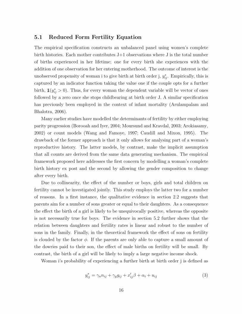
5.1 Reduced Form Fertility Equation

The empirical specification constructs an unbalanced panel using women’s complete

birth histories. Each mother contributes J+1 observations where J is the total number

of births experienced in her lifetime; one for every birth she experiences with the

addition of one observation for her entering motherhood. The outcome of interest is the

unobserved propensity of woman i to give birth at birth order j, y⇤ij. Empirically, this is

captured by an indicator function taking the value one if the couple opts for a further

birth, (y⇤ij > 0). Thus, for every woman the dependent variable will be vector of ones

followed by a zero once she stops childbearing at birth order J. A similar specification

has previously been employed in the context of infant mortality (Arulampalam and

Bhalotra, 2006).

Many earlier studies have modelled the determinants of fertility by either employing

parity progression (Borooah and Iyer, 2004; Moursund and Kravdal, 2003; Arokiasamy,

2002) or count models (Wang and Famoye, 1997; Caudill and Mixon, 1995). The

drawback of the former approach is that it only allows for analysing part of a woman’s

reproductive history. The latter models, by contrast, make the implicit assumption

that all counts are derived from the same data generating mechanism. The empirical

framework proposed here addresses the first concern by modelling a woman’s complete

birth history ex post and the second by allowing the gender composition to change

after every birth.

Due to collinearity, the e↵ect of the number or boys, girls and total children on

fertility cannot be investigated jointly. This study employs the latter two for a number

of reasons. In a first instance, the qualitative evidence in section 2.2 suggests that

parents aim for a number of sons greater or equal to their daughters. As a consequence

the e↵ect the birth of a girl is likely to be unequivocally positive, whereas the opposite

is not necessarily true for boys. The evidence in section 5.2 further shows that the

relation between daughters and fertility rates is linear and robust to the number of

sons in the family. Finally, in the theoretical framework the e↵ect of sons on fertility

is clouded by the factor �. If the parents are only able to capture a small amount of

the dowries paid to their son, the e↵ect of male births on fertility will be small. By

contrast, the birth of a girl will be likely to imply a large negative income shock.

Woman i’s probability of experiencing a further birth at birth order j is defined as

y

⇤ij = �nnij + �ggij + x

0ij� + ↵i + uij (3)

16

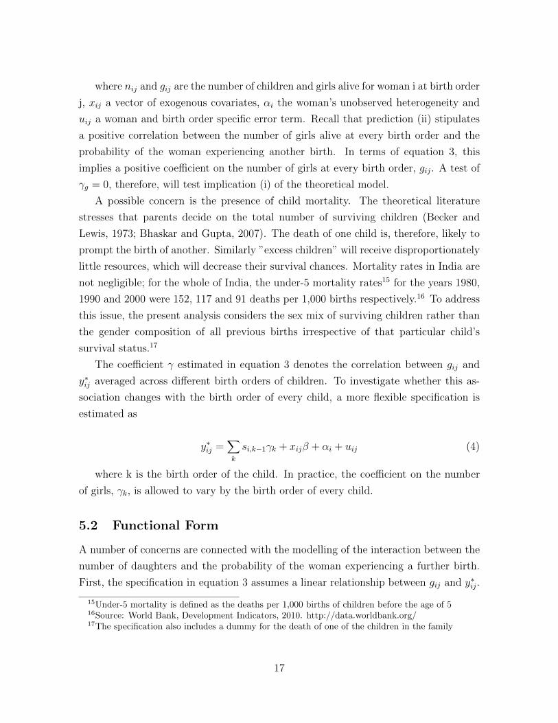
where nij and gij are the number of children and girls alive for woman i at birth order

j, xij a vector of exogenous covariates, ↵i the woman’s unobserved heterogeneity and

uij a woman and birth order specific error term. Recall that prediction (ii) stipulates

a positive correlation between the number of girls alive at every birth order and the

probability of the woman experiencing another birth. In terms of equation 3, this

implies a positive coe�cient on the number of girls at every birth order, gij. A test of

�g = 0, therefore, will test implication (i) of the theoretical model.

A possible concern is the presence of child mortality. The theoretical literature

stresses that parents decide on the total number of surviving children (Becker and

Lewis, 1973; Bhaskar and Gupta, 2007). The death of one child is, therefore, likely to

prompt the birth of another. Similarly ”excess children” will receive disproportionately

little resources, which will decrease their survival chances. Mortality rates in India are

not negligible; for the whole of India, the under-5 mortality rates15 for the years 1980,

1990 and 2000 were 152, 117 and 91 deaths per 1,000 births respectively.16 To address

this issue, the present analysis considers the sex mix of surviving children rather than

the gender composition of all previous births irrespective of that particular child’s

survival status.17

The coe�cient � estimated in equation 3 denotes the correlation between gij and

y

⇤ij averaged across di↵erent birth orders of children. To investigate whether this as-

sociation changes with the birth order of every child, a more flexible specification is

estimated as

y

⇤ij =

X

k

si,k�1�k + xij� + ↵i + uij (4)

where k is the birth order of the child. In practice, the coe�cient on the number

of girls, �k, is allowed to vary by the birth order of every child.

5.2 Functional Form

A number of concerns are connected with the modelling of the interaction between the

number of daughters and the probability of the woman experiencing a further birth.

First, the specification in equation 3 assumes a linear relationship between gij and y

⇤ij.

15Under-5 mortality is defined as the deaths per 1,000 births of children before the age of 516Source: World Bank, Development Indicators, 2010. http://data.worldbank.org/17The specification also includes a dummy for the death of one of the children in the family

17

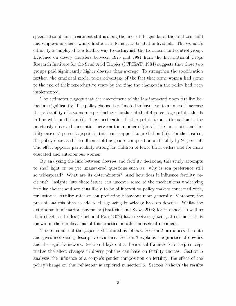
To investigate this linearity assumption, equation 3 is re-estimated using a dummy for

every girl born as

y

⇤ij =

X

k

Dk k + xij� + ↵i + uij (5)

where Dk is an indicator variable taking the value 1 if the number of surviving girls

equals to k. The parameter estimates of k along with a histogram for the fraction of the

number of girls alive in each family in the sample are shown in Figure 3. For values of

the explanatory variable between 1 and 6, the dashed line suggests a linear relationship

between the number of girls alive and the probability of the woman experiencing a

further birth.18

Second, the specification in equation 3 assumes that parents’ only criterion for

reproductive decisions is the number of girls alive. Parents may, however, take other

factors into account - take the ratio of sons to daughters, for example. As a consequence,

controlling for these alternative factors may alter the correlation between daughters

and fertility significantly. To address this concern, equation 5 is re-estimated with the

inclusion of variables accounting for the gender composition of the child’s siblings; a

dummy for more boys than girls in the family and one for the opposite case. The

parameter estimates for the number of daughters on fertility are reported in figure 3 as

the dotted line. They show that the inclusion of variables approximating the gender

composition of the household does not change the correlation between the number of

daughters and fertility significantly. The dotted line is very similar to the dashed line

for the model without these controls.

6 The E↵ect of Dowries on Fertility Decisions

The empirical modelling of the e↵ect of marital payments on fertility decisions - outlined

in implications (i) and (iii) - is complicated by the fact that there is little information

on these transfers. In addition, decisions on marital transfers are likely to be deter-

mined jointly with reproductive and other family-related decisions. Finally, current

dowry payments are only error prone measures of parents’ expectations regarding fu-

ture dowries. To isolate the causal e↵ect of anticipated dowries on fertility decisions,

this study exploits the major revision in anti dowry laws outlined in section 3.2.

18The percentage of women with more than 6 girls alive is around 1%.

18

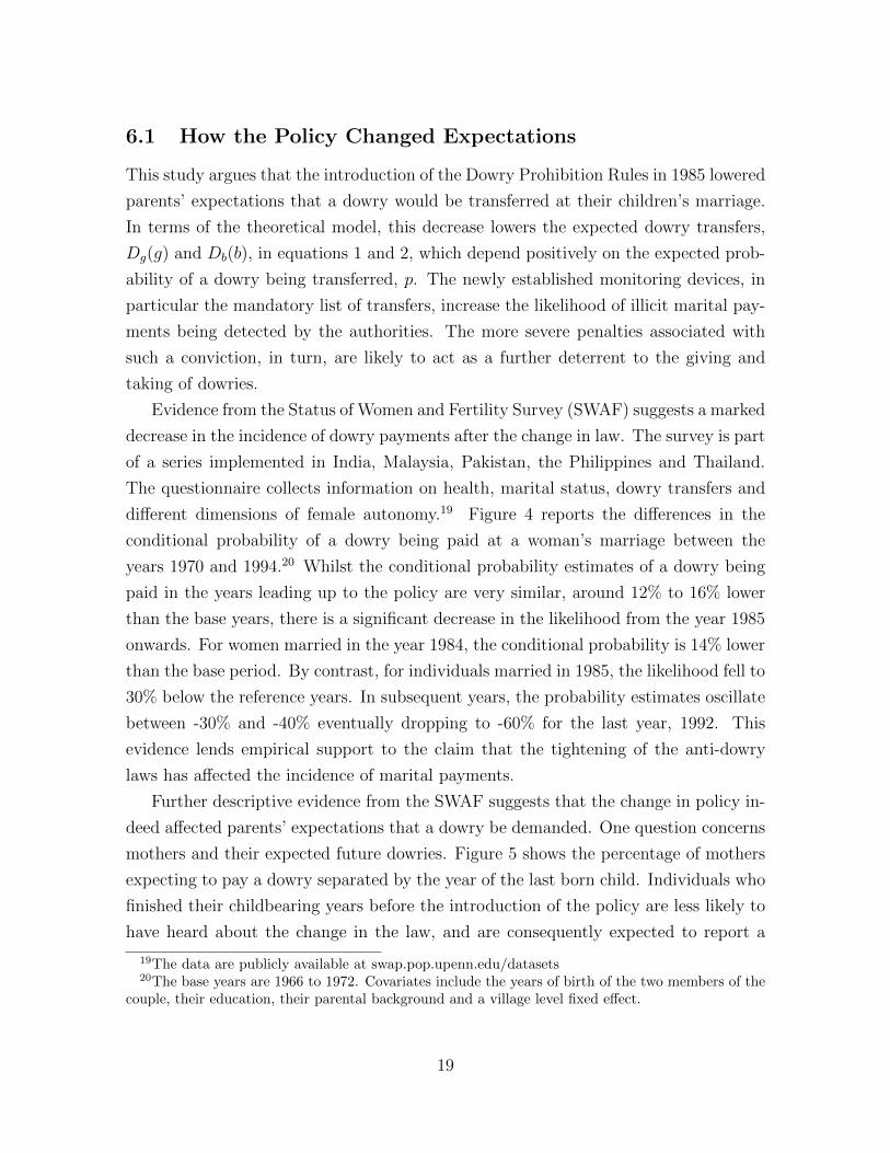
6.1 How the Policy Changed Expectations

This study argues that the introduction of the Dowry Prohibition Rules in 1985 lowered

parents’ expectations that a dowry would be transferred at their children’s marriage.

In terms of the theoretical model, this decrease lowers the expected dowry transfers,

Dg(g) and Db(b), in equations 1 and 2, which depend positively on the expected prob-

ability of a dowry being transferred, p. The newly established monitoring devices, in

particular the mandatory list of transfers, increase the likelihood of illicit marital pay-

ments being detected by the authorities. The more severe penalties associated with

such a conviction, in turn, are likely to act as a further deterrent to the giving and

taking of dowries.

Evidence from the Status of Women and Fertility Survey (SWAF) suggests a marked

decrease in the incidence of dowry payments after the change in law. The survey is part

of a series implemented in India, Malaysia, Pakistan, the Philippines and Thailand.

The questionnaire collects information on health, marital status, dowry transfers and

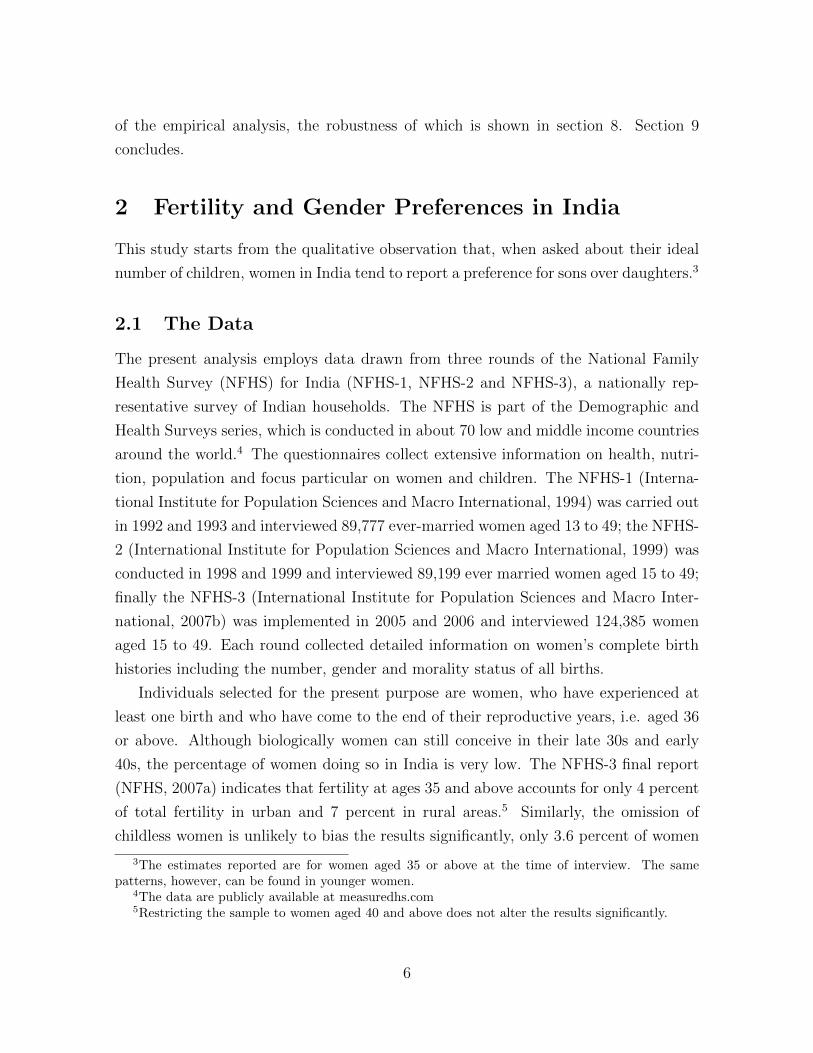
di↵erent dimensions of female autonomy.19 Figure 4 reports the di↵erences in the

conditional probability of a dowry being paid at a woman’s marriage between the

years 1970 and 1994.20 Whilst the conditional probability estimates of a dowry being

paid in the years leading up to the policy are very similar, around 12% to 16% lower

than the base years, there is a significant decrease in the likelihood from the year 1985

onwards. For women married in the year 1984, the conditional probability is 14% lower

than the base period. By contrast, for individuals married in 1985, the likelihood fell to

30% below the reference years. In subsequent years, the probability estimates oscillate

between -30% and -40% eventually dropping to -60% for the last year, 1992. This

evidence lends empirical support to the claim that the tightening of the anti-dowry

laws has a↵ected the incidence of marital payments.

Further descriptive evidence from the SWAF suggests that the change in policy in-

deed a↵ected parents’ expectations that a dowry be demanded. One question concerns

mothers and their expected future dowries. Figure 5 shows the percentage of mothers

expecting to pay a dowry separated by the year of the last born child. Individuals who

finished their childbearing years before the introduction of the policy are less likely to

have heard about the change in the law, and are consequently expected to report a

19The data are publicly available at swap.pop.upenn.edu/datasets20The base years are 1966 to 1972. Covariates include the years of birth of the two members of the

couple, their education, their parental background and a village level fixed e↵ect.

19

stronger willingness to pay dowries in the future. This is borne out by the descriptive

evidence shown here, where the percentage of women intending to pay a dowry in the

future increases steadily until the introduction of the policy. After the policy change,

by contrast, the fraction decreases.

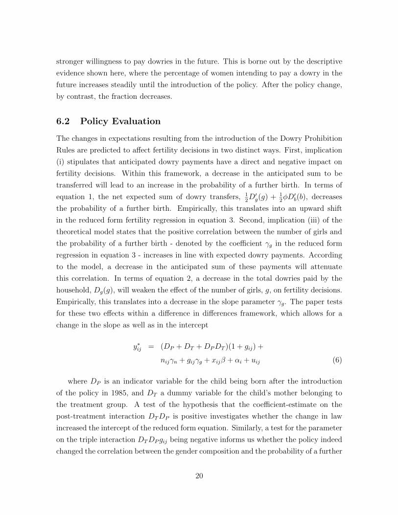
6.2 Policy Evaluation

The changes in expectations resulting from the introduction of the Dowry Prohibition

Rules are predicted to a↵ect fertility decisions in two distinct ways. First, implication

(i) stipulates that anticipated dowry payments have a direct and negative impact on

fertility decisions. Within this framework, a decrease in the anticipated sum to be

transferred will lead to an increase in the probability of a further birth. In terms of

equation 1, the net expected sum of dowry transfers, 12D

0g(g) +

12�D

0b(b), decreases

the probability of a further birth. Empirically, this translates into an upward shift

in the reduced form fertility regression in equation 3. Second, implication (iii) of the

theoretical model states that the positive correlation between the number of girls and

the probability of a further birth - denoted by the coe�cient �g in the reduced form

regression in equation 3 - increases in line with expected dowry payments. According

to the model, a decrease in the anticipated sum of these payments will attenuate

this correlation. In terms of equation 2, a decrease in the total dowries paid by the

household, Dg(g), will weaken the e↵ect of the number of girls, g, on fertility decisions.

Empirically, this translates into a decrease in the slope parameter �g. The paper tests

for these two e↵ects within a di↵erence in di↵erences framework, which allows for a

change in the slope as well as in the intercept

y

⇤ij = (DP +DT +DPDT )(1 + gij) +

nij�n + gij�g + xij� + ↵i + uij (6)

where DP is an indicator variable for the child being born after the introduction

of the policy in 1985, and DT a dummy variable for the child’s mother belonging to

the treatment group. A test of the hypothesis that the coe�cient-estimate on the

post-treatment interaction DTDP is positive investigates whether the change in law

increased the intercept of the reduced form equation. Similarly, a test for the parameter

on the triple interaction DTDP gij being negative informs us whether the policy indeed

changed the correlation between the gender composition and the probability of a further

20

birth denoted by the coe�cient �g.

Because the policy changes outlined in section 3.2 were introduced in the whole

country simultaneously, geographical variation cannot be employed to identify the e↵ect

of the policy on reproductive decisions. Instead, the analysis exploits the heterogeneity

of dowry payments before the implementation of the Dowry Prohibition Rules in order

to argue that the e↵ect of the policy varies according to the average amount of dowries

paid by households before its introduction. In particular, it maintains that the policy

change had a more pronounced impact on households paying particularly high dowries

prior to 1985; these individuals are the treatment group. By contrast, households

paying on average low dowries are unlikely to have been a↵ected by the change in

law; these individuals are the control group. The present analysis evaluates the Dowry

Prohibition Rules by comparing mothers with a firstborn son to women whose firstborn

child is female. To further strengthen the results, the specification exploits variation

by the mother’s caste as well as by her birth cohort.

6.2.1 Variation by Gender of Firstborn Child

Families with a firstborn daughter are more likely to have been a↵ected by the Dowry

Prohibition Rules than couples with a firstborn son for two reasons. First, the gender of

the firstborn child is likely to influence the total amount of dowry transfers paid by the

parents. There is a strong and positive correlation between the number of daughters in

the family and the total sum of a given household’s dowry expenditures. Families with

a firstborn daughter are more likely to have a higher number of girls because of the

gender of the child itself on the one hand, and by increasing fertility levels on the other

hand. Second, the gender of the firstborn is likely to determine the timing of dowry

payments. If the oldest child in the family is a girl, the negative income shock resulting

from her dowry payment is likely to occur before any positive income streams deriving

from, for instance, sons’ dowries or remittances. The fact that age at first marriage

is relatively low in India exacerbates this. The gender of the firstborn child has been

increasingly employed in past studies to approximate for parental fertility as well as

for the gender composition of children (Rosenblum, 2013; Jensen, 2003; for instance).

In terms of the theoretical framework, inequality 2 states that households with a

large number of daughters are more likely to have expenditures on children in excess of

En. The decrease in expected dowries is likely to bring some of these families below En

and thus have a stronger impact on fertility than on households with a predominantly

21

male o↵spring. The gender of the first child can be seen as an approximation of the

number of daughters alive at the introduction of the Dowry Prohibition Rules. Column

(1) in table 2 shows that in the sample at hand the gender of the firstborn child strongly

influences the gender composition of children born to women in India. The parameter

estimates indicate that the birth of a girl at birth order one increases the ratio of girls

at the end of the woman’s reproductive life by 32%.21

Descriptive evidence from the ICRISAT data on dowry transfers between 1975

and 1984 lends weight to the positive correlation between the women residing in the

household and the total amount of dowry payments by the household. Columns (2)

and (3) of Table 1 show that household in which a daughter married during the sample

period show a higher proportion of dowry transfers, 87 percent, compared to households

where such an event did not take occur, 74 percent. Furthermore, the marriage of a

daughter increases the net amount of dowries paid out by the household; 1,115 Rupees

per year compared to 721 Rupees, see row (f). When compared to the households’

consumption on non-durables in row (h), the di↵erence is stark, 72 versus 33 percent.

Note that these figures consider the overall gender composition of the household and

not just the gender composition of the o↵spring, and can thus only be seen as suggestive

evidence.

A possible concern with this empirical strategy is the exogeneity of the sex of the

firstborn child. The presence of sex selective abortions in India at birth order one is

debated. Whilst Jha et al. (2006) argue for the presence of this practice even at the first

birth, Retherford and Roy (2003) and more recently Poertner (2010) and Rosenblum

(2013) have shown that sex ratios at birth lie within normal limits. Descriptive evidence

from the three rounds of the NFHS appears to lend support to the exogeneity of

the sex of the first born child. Table 2 shows the sex ratio at birth and di↵erences

in socio-economic characteristics for women with a firstborn son versus a firstborn

daughter. In Row (a), the percentage of girls born at birth order one for the sample

at hand, 47.9, is very close to the one predicted by the natural rate shown in row (b).

Columns (2) and (3) report the characteristics of parents by the gender of their firstborn

child. The di↵erences appear negligible. The only statistical significantly di↵erent

variables are the percentage of women with primary education and the mother’s age

at first birth. However, the magnitudes of these di↵erences appear very small, 1.1%

for maternal education and 0.1 years for the age at first birth. Column (5) of Table 2

21The magnitude of the estimate is in line with what reported by Rosenblum (2013)

22

shows the parameter estimates of the regression of the firstborn’s gender on parental

characteristics. The mother’s education and age at birth are significantly correlated

with the gender of the firstborn son. Akin to above, the parameter estimates do not

appear very large, 0.007 for the former and 0.001 for the latter. The low R-squared

further points to the exogeneity of the firstborn’s gender. A possible reason for these

findings is that ultrasound technology was not widely available in the mid 1980s. This

notion will be explored further in section 8.

6.2.2 Variation by Ethnicity

There are two reasons why dowries weigh more heavily on the budget of low caste

compared to that of high caste families. On the one hand, individuals belonging to

lower castes tend to exhibit worse socio-economic outcomes. The government of India

explicitly recognises this and classifies scheduled castes, tribes and other castes as

historically disadvantaged groups of society, which are to be given special provisions.22

Academic work has also pointed to similar di↵erences (Deshpande, 2000; for instance).

On the other hand, lower caste status is seen as an unattractive feature in a bride

(see Anderson, 2003; for a theoretical model). As a consequence, parents of lower

castes are likely to have to pay higher dowries than higher caste members to attract

husbands of the same quality, ceteris paribus. In fact, the growing importance of

dowries for the budget of lower caste households has been documented. Whilst the

practice originated among members of the highest caste Brahmins, and Rao (1993) finds

a positive correlation between a household’s caste rank and dowries, more recent work

points out that lower caste members started paying disproportionately high dowries in

an e↵ort to copy the higher castes (Srinivas, 1997).

In terms of the theoretical framework, one can think of the low budget available

to lower castes as translating into higher dowry payments Dg(g) without necessarily

generating higher dowry revenues, �Db(b). Evidence from the ICRISAT confirms that

marital payments weigh more on the budget of lower caste than higher caste households.

Columns (4) and (5) of table 1 show that, lower caste households exhibit a higher

probability of paying dowries, 84 versus 80 percent. Furthermore, although the caste

of the household does not appear to influence the inflow of dowry payments, lower

caste households appear to show considerably higher out payments of dowries. This

22The a�rmative action of the ”Reservation Policy” in India is an example of policies aimed explic-itly at the lower castes.

23

translates into considerably larger net dowry payments for these households, 2,539

Rupees per year compared to 216 Rupees per year for higher caste households.

6.2.3 Variation by Birth Cohort of Mother

To further strengthen the two sets of results laid out in sections 6.2.1 and 6.2.2, this

study exploits the fact that some women had come to the end of their reproductive

years by the time the Dowry Prohibition Rules were introduced in 1985. Women born

between the years 1954 and 1970 were aged 15 to 31 at the implementation of the

policy change. These individuals are assumed to be strongly a↵ected by the policy.

By contrast, mothers born between 1942 and 1948 were aged 37 to 43 at the time of

the policy change and thus less likely to have been a↵ected by the change in the law.

Referring only to information from the latter group, the empirical analysis evaluates

a fictional policy in the year 1971, using the two methodologies outlined above to test

the hypothesis that the policy had a negligible e↵ect on fertility decisions.

7 Results

The empirical models laid out in sections 5 and 6.2 are estimated using completed

birth histories drawn from three rounds of the National Family Health Survey for

India. Section 2.1 describes the data employed in detail. The dependent variable is the

unobserved probability of the woman experiencing a further birth at every birth order.

The specifications control for the number of girls and children alive and sequentially

add a time trend, maternal and paternal characteristics as well as a mother-level fixed

e↵ect.

7.1 Gender Composition of Children and Fertility Choices

The estimates of the empirical framework outlined in equation 3 show a strong pos-

itive correlation between the number of daughters alive at every birth order and the

probability of a subsequent birth. This lends support to prediction (ii), i.e. the pos-

itive correlation between the number of daughters alive at every birth order and the

probability of a subsequent birth. A birth (and survival) of a girl is associated with a

5 to 7 percentage point increase in the probability of the woman experiencing a fur-

ther birth. This finding is in congruence with the large number of studies reported

24

in the introduction pointing out the strong influence of gender preferences on fertility

decisions in India and Southeast Asia.

The relative magnitudes of �n (the coe�cient on the number of children) and �g

(the coe�cient on the number of girls) shed further light on the way in which the

gender composition of a couple’s o↵spring influences its fertility decisions. For the

preferred specification in column (5), the magnitudes of the two parameter estimates

are of similar size, -0.101 for �n and 0.068 for �g. This suggests that the negative

influence of a further birth on subsequent fertility is almost completely outweighed by

the positive e↵ect of the delivery of a girl. A possible explanation for this fact is that

parents aim for a particular number of boys as pointed out by Yamaguchi (1989) and

Jensen (2003).

The very small parameter estimates on the square of the number of children alive

at every birth order (between 0.000 and 0.005) suggest that the correlation between

this covariate and y

⇤ij is close to linear. Finally and as expected, the mother’s age at

the birth of every child, shows a consistently negative correlation with the likelihood

of that woman experiencing a further birth.

Figure 6 shows the parameter estimates based on equation 4 in which the parameter

on the number of girls, �g, is allowed to vary with the birth of every child. The plot

suggests that the correlation between the number of girls alive and fertility decisions

varies considerably throughout a woman’s reproductive life. The correlation shows

an inversely U shaped pattern where the association between gij and y

⇤ij increases for

birth orders one to three from close to 0 to 0.09. After this birth order, the coe�cient

estimates begin to decrease reaching a very small estimate again for birth order eight.

A possible explanation for these results is that the gender composition of the o↵spring

matters most to parents as they approach their ideal family size, which lies between 2

and 4.

7.2 Dowries and Fertility Decisions

In line with predictions (i) and (iii), the decrease in expected dowry payments resulting

from the introduction of the Dowry Prohibition Rules is found to lead to a one-o↵

increase in fertility as well as to an attenuation in the previously observed correlation

between the gender composition of a couple’s o↵spring and its fertility choices.

25

7.2.1 Results based on the Gender of the Firstborn Child

Rows (a), (b) and (c) of table 4 report the coe�cients on the di↵erence in di↵erences

dummy variables. The estimates reported in row (a) suggest that fertility decreased

for the control group over time; the figures in row (b) that before the introduction of

the policy, families with a firstborn girl are more likely to give birth. The interaction

between the post and treatment dummies is positive and significant. The decrease in

expected dowries resulting from the policy change is thus estimated to have increased

the chances of a further birth by between 2 and 4 percentage points, which supports

prediction (i), i.e. the positive relation between the expected level of dowries to be

paid and the probability of the couple opting for a further birth.

The figures reported in row (d) of table 4 suggest that before the policy change

the control group exhibited a positive correlation between gij and y

⇤ij. The parameter

estimates for the number of girls alive range from 0.02 to 0.03. Rows (e) to (g) report

the coe�cients on the number of daughters alive (variable gij in equation 6) interacted

with the di↵erence in di↵erences indicator variables. The estimates in row (e) indicate

that, for the control group, the influence of the number of girls increased over time.

The positive coe�cients in row (f) point to this correlation in the pretreatment period

to have been stronger for couples with a firstborn daughter. The magnitude of the

di↵erence is estimated between 0.04 and 0.06. This finding lends support to the claim

that the gender of the first child adequately distinguishes treated from untreated indi-

viduals. Recall that treatment status depends on the amount of dowries paid before

the introduction of the policy. If a sub-sample pays particularly high dowries before the

change in the law, one would expect these individuals to exhibit a stronger correlation

between gij and y

⇤ij (see equation 3). The positive and significant coe�cient estimates

of row (f) show this to be the case for couples with a firstborn daugher.

The coe�cient estimates on the triple interaction between the number of girls alive,

gij, the post and the treatment dummies shown in row (g) report how the coe�cient �g

changed as a result of the introduction of the Dowry Prohibition Rules; this coe�cient

can be thought of as the di↵erence in the di↵erences in the slope parameter �g, i.e.

the correlation between the number of girls alive and fertility rates. The estimates

show that the correlation decreased by between 4 and 5 percentage points, which lends

support to prediction (iii), i.e. that the positive correlation between the gender com-

position and fertility choices is increasing in expected future dowries. The coe�cient

estimates in rows (d) to (g) for the preferred specification in column (5) can be used to

26

calculate that, for the control group, the coe�cient �g increased from 0.027 to 0.055.

For the treatment group, by contrast, it decreased from 0.085 to 0.068.

7.2.2 Results based on Ethnicity

Table 5 reports the di↵erence in di↵erences estimates employing the woman’s ethnicity

to distinguish treatment and control group. Rows (a) and (b) suggest that fertility

increased for the control group over time but do not show a substantial di↵erence

between treatment and control before the policy. The parameter estimates in row (c)

indicate that the policy increased the probability of a further birth by between 4 and

6 percentage points.

Row (d) confirms the positive correlation between gij and y

⇤ij for the control group

prior to the introduction of the Dowry Prohibition Rules. Row (e) suggests that this

correlation decreased over time. The coe�cient estimates in row (f) show that before

the policy was introduced, the correlation between the number of girls alive at every

birth order and the probability of a further birth was significantly larger for lower

caste members. The estimates for this di↵erence range from 0.01 to 0.27. As stated

in the previous section, these estimates support the claim that treated and untreated

individuals are adequately distinguished. The estimates in row (g) suggest that the

policy decrease the coe�cient �ij by between 1 and 2 percentage points, which - akin

to above - supports prediction (iii). Post estimation calculations further show that, for

the control group the coe�cient �ij decreased from 0.103 to 0.052. For the treatment

group the decrease was more pronounced, from 0.130 to 0.058.

7.2.3 Results based on older cohorts

Table 6 reports the estimates of equation 6 carried out for women born between 1942

and 1948 with a fictional policy in the year 1971. Row (a) shows that, for women with

a firstborn daughter, the fictional policy did not change the intercept. The estimates of

the five di↵erent specifications are small in size and not significantly di↵erent from zero.

Row (b) confirms the positive correlation between the number of daughters alive and

the probability of a further birth for the control group in the pre-treatment period. As

row (c) shows, however, the fictional policy did not a↵ect the slope parameter associated

with this variable. The triple interaction terms are small and not significantly di↵erent

from zero. The estimates using the woman’s ethnicity shown in rows (d) to (f) paint a

very similar picture. For this specification, however, the fictional policy of 1971 a↵ected

27

the intercept of the estimating equation by between 0.05 and 0.07. The slope of the

coe�cient �g, by contrast, remains unchanged by the placebo treatment.

7.3 Treatment Heterogeneity

Figure 7 reports the parameter estimates of an extended version of equation 6, which

allows for the impact of the policy to vary with the birth order of the child. The schedule

shows the changes in the slope parameter only and indicates that the strongest impact

of the policy occurs at birth orders 2 and 3. For the control group, the coe�cient �g

hardly changed at birth orders 2 and 3. For the treatment group, by contrast, the

parameter estimates dropped from 0.09 to 0.03 at birth order 2 and from 0.14 to 0.1

at birth order 3. Since the frequency of these birth orders is very high (see figure 6),

this behaviour has a strong impact on the overall sample.

Table 7 reports how the impact of the policy change varies by the characteristics

of the mother. Columns (1) to (4) show the impact of the Dowry Prohibition Rules

distinguishing by the mother’s region of residence. The parameter estimates suggest

that the largest change in behaviour occurred in the West and North of India. In

these two locations, the policy lead to an increase in the intercept of 0.057 and 0.042

respectively. The parameter �g further decreased by -0.053 in the West and -0.036 in

the North. By contrast, in the South of India women hardly reacted to the policy. This

last finding is in congruence with previous research highlighting the less widespread

custom of dowries in the South. Columns (5) and (6), moreover, suggest a clear posi-

tive correlation between the impact of the Dowry Prohibition Rules and the mother’s

education. Although the change in the intercept is similar for women with and without

completed primary education (0.042 and 0.04, respectively), the slope parameter for

the former group decreased by -0.06 whereas for the latter it was only attenuated by

-0.036. One possible explanation for this finding is that women with higher levels of ed-

ucation are likely to have higher levels of autonomy. The resulting improved agency is

likely to enable these individuals to respond more e↵ectively to the new circumstances

by a↵ecting decisions taken by the household as a whole.

In order to investigate the relative importance of female autonomy on the e�ciency

of the policy, this study employs two measurements previously argued to approximate

this concept. Abadian (1996) argues that women who marry at an early age and have a

large age di↵erence to their husband show low female autonomy. The results reported

in columns (7) to (10) suggest that more autonomous women responded more strongly

28

to the Dowry Prohibition Rules. Women whose age at marriage lies above the sample

average show larger intercept and slope changes, see columns (7) and (8). Similarly,

women with age di↵erences to their husbands that lie below the sample mean show the

same pattern.

8 Robustness Checks

8.1 Placebo Treatments

To address the concern that the post 1985 dummy is correlated with changes in fertility

behaviour unrelated to the influence of the Dowry Prohibition Rules a number of

falsification tests are carried out. Columns (1) to (4) of Table 8 specify two di↵erent

placebo treatments between the years 1976 and 1984 as well as between 1979 and 1984.

In addition to these variables, the specification retains the post 1985 dummies and their

interactions, which will test whether the post-treatment e↵ect is robust to di↵erent

reference time periods. Rows (a) and (b) show that, although the placebo treatment

changes the intercept of the reduced form fertility equation, the shift appears negligible

when compared results of the post 1985 dummies reported in rows (c) and (d); 0.016

and 0.021 versus 0.052 and 0.048 for the specification employing the gender of the

firstborn and 0.024 and 0.036 versus 0.070 and 0.073 for the specification employing

the mother’s caste. Furthermore, rows (f) and (g) show that the placebo treatment did

not change the slope parameter �g significantly. The parameter estimates are small in

size and not statistically significant. The estimates for the post 1985 dummy in rows

(h) and (i), by contrast, remain large, negative and significant; column (3) being the

exception.

8.2 Sex Selective Abortions

A further point of concern is the presence of sex selective abortions. This practice gives

parents the possibility of responding to changes in expected dowries by influencing the

gender of each child rather than by changing their fertility patterns. As mentioned

before, the extent of this practice is debated.23 Figure 8 plots the percentage of girls

born per birth year in the post period.24 The upper panel divides the sample by the

23See section 6.2.1.24Recall that the natural percentage of girls at birth is 48.8%.

29

gender of the firstborn child, the bottom panel by the woman’s ethnicity.25 In both

panels, it is hard to detect any systematic di↵erences in the sex ratio at birth between

treatment and control group. Furthermore, in the upper panel the only year in which

there is a statistical di↵erence between the treatment and control group is 1994; for the

bottom panel, only for the years 1989 and 1998. This suggests that neither the gender

of the first born or the mother’s caste introduce di↵erences in sex selective abortions.

8.3 Di↵erent Post Treatment Periods

Children in the estimation sample are born between the years 1970 and 2001. This

relatively long time window raises the concern that factors independent of the pol-

icy change influence the results. Columns (5) to (10) of table 8 report the di↵erence

in di↵erences estimates employing di↵erent time windows for the post treatment pe-

riod. The three time spans are 1985 to 1995, 1985 to 1990 and 1985 to 1986. The

parameter estimates show that the estimation is robust to di↵erent definitions of the

post-treatment window. In both specifications, the intercept shift remains positive and

significant. Similarly, the change in the slope continues to be negative, significant and

of similar magnitude.

These results can also be interpreted as evidence in favour of the claim that sex

selective abortions are unlikely to bias the results. As mentioned by Bhalotra and

Cochrane (2010) sex detection technology was scarce and expensive in the mid-1980s

in India. The fact that the results remain stable to the employment of children born

only in this decade suggests that parents adopted to the change in policy by adjusting

their fertility behaviour rather than by employing sex selective abortions.

8.4 Common Time Trends

The causal interpretation of the di↵erence in di↵erences estimates relies on the as-

sumption of orthogonality between the Dowry Prohibition Rules and the error term.

Figure 9 explores the fertility behaviour of women born between the years 1942 and

1953 to give suggestive evidence in favour of the aforementioned assumption. These

individuals were aged 32 to 43 at the implementation of the policy change and are thus

assumed to only have been marginally a↵ected by it. The negative slope of both curves

highlights the well-documented fertility decline in India. The upper panel of figure 9

25For the upper hand panel only children of birth order 2 or above are considered.

30

opposes women with a firstborn son to mothers, whose firstborn is female. Although

individuals in the latter group show higher fertility levels, the gender of the first child

does not appear to change the rate of change in fertility behaviour significantly. The

lower panel contrasts women from lower and higher castes. Akin to before, whilst the

former show consistently higher fertility levels, the slope of both schedules appears

similar.

9 Conclusion

The main results of this paper suggest that the widely documented correlation between

a couple’s gender composition and its fertility choices is, in part, a reflection of gen-

der di↵erences in the economic costs of children. Two ramifications of these findings

appear of particular interest. First, the relative importance of child raising costs for

parents’ reproductive behaviour raises the question whether economic factors also in-

fluence other aspects of raising children. Whilst researchers are devoting increasing

interest to inheritance rights or political representation of women, human development

aspects such as nutrition, weight, height and other health outcomes have remained

underexplored. Second, many previous explanations of the presence of son preferring

stopping rules in fertility behaviour argued for these being the result of deeply rooted

attitudes that somehow boys are more valuable than girls. The results put forward

here, by contrast, argue that a large part of this behaviour can explained by the rela-

tively simple economic intuition that sons are cheaper to raise than girls. Moreover, if

dowries a↵ect reproductive behaviour it stands to reason that other factors influencing

the net cost of children - may it be the cost or returns - can potentially influence the

same processes. This is an encouraging finding for practitioners because it can con-

stitute a new set of instruments to influence fertility decisions taken by households.

Furthermore, from a political perspective, dowries have been widely criticised for their

negative influence on brides. This analysis highlights a further negative unintended

consequence of this already widely criticised custom. As a consequence, any policy

counteracting dowries will have a spillover e↵ect on couple’s reproductive behaviour

thus further increasing the need to counteract this practice.

31

References

Abadian, S., “Women’s autonomy and its impact on fertility,” World Development,

1996, 24 (12), 1793 – 1809.

Anderson, S., “Why Dowry Payments Declined with Modernization in Europe but

Are Rising in India?,” The Journal of Political Economy, 2003, 111 (2), 269 – 310.

, “The Economics of Dowry and Brideprice,” Journal of Economic Perspectives,

2007, 21 (4), 151 – 174.

, “Why the marriage squeeze cannot cause dowry inflation,” Journal of Economic

Theory, 2007, 137 (1), 140 – 152.

Angrist, J. and W. N. Evans, “Children and their parents labor supply: Evidence

from exogenous variation in family size,” American Economic Review, 1998, 88 (3),

450 – 477.

Arnold, F., M. K. Choe, and T. K. Roy, “Son Preferences, the Family Building

Process and Child Mortality in India,” Population Studies, 2002, 52, 301 – 315.

Arokiasamy, P., “Gender Preference, Contraceptive Use and Fertility in India: Re-

gional and Development Influences,” International Journal of Population Geography,

2002, 8 (1), 49 – 67.

Arulampalam, W. and S. Bhalotra, “Sibling Death Clustering in India: State De-

pendence Versus Unobserved Heterogeneity,” Journal of the Royal Statistical Society,

2006, 169 (4), 829 – 848.

Arunachalam, R. and T. Logan, “Is there dowry inflation in India?,” NBER Work-

ing Paper No. 13905, 2008.

Barcellos, S. H., L. Carvalho, and A. Lleras-Muney, “Child Gender and Parental

Investment in India: Are Boys and Girls Treated Di↵erently?,” NBER Working

Paper Series, 2012, 17781.

Becker, G. and H. G. Lewis, “On the Interaction between the Quantity and Quality

of Children,” Journal of Political Economy, 1973, 81, 279S288.

32

Bhalotra, S. and T. Cochrane, “Where have all the young girls gone? Identification

of Sex Selection in India,” IZA Working Paper, 2010, 5381.

Bhargava, A., “Family Planning, Gender Di↵erences and Infant Mortality: Evidence

from Uttar Pradesh, India,” Journal of Econometrics, 2003, 112, 225 – 240.

Bhaskar, V. and B. Gupta, “India’s missing firls: biology, customs, and economic

development,” Oxford Review of Economic Policy, 2007, 23 (2), 221 – 238.

Bloch, F. and V. Rao, “Terror as a Bargaining Instrument: A Case Study of Dowry

Violence in Rural India,” American Economic Review, 2002, 92 (4), 1029 – 1043.

Borooah, V. and S. Iyer, “Religion and Fertility in India: The Role of Son Prefer-

ences and Daughter Aversion,” Cambridge Working Papers, 2004.

Botticini, M. and A. Siow, “Why Dowries?,” American Economic Review, 2003, 93

(4), 1385 – 1398.

Caldwell, J. C:, P. H. Reddy, and P. Caldwell, “The causes of marriage change

in South India,” Population studies, 1983, 37 (3), 343 – 361.

Caudill, S. B and F. G. Mixon, “Modeling Household Fertility Decisions: Esti-

mation and Testing Censored Regression Models for Count Data,” Empirical Eco-

nomics, 1995, 20, 183 – 196.

Clark, S., “Son Preference and Sex Composition of Children: Evidence from India,”

Demography, 2000, 37 (1), 95 – 108.

Dahl, G. B. and E. Moretti, “The Demand for Sons,” The Review of Economic

Studies, 2008, 75, 1085 – 1120.

Dalmia, Sonia, “A hedonic analysis of marriage transactions in India: estimating

determinants of dowries and demand for groom characteristics in marriage,” Research

in Economics, 2004, 58, 235 – 255.

Deolalikar, A. and V. Rao, The demand for dowries and bride characteristics in

marriage: Empirical estimates from rural South-Central India, Oxford University

Press, 1998.

33

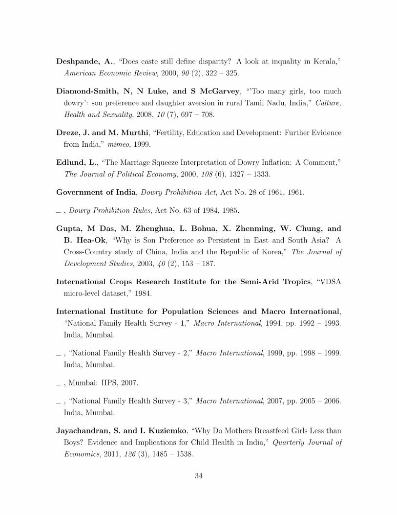
Deshpande, A., “Does caste still define disparity? A look at inquality in Kerala,”

American Economic Review, 2000, 90 (2), 322 – 325.

Diamond-Smith, N, N Luke, and S McGarvey, “’Too many girls, too much

dowry’: son preference and daughter aversion in rural Tamil Nadu, India,” Culture,

Health and Sexuality, 2008, 10 (7), 697 – 708.

Dreze, J. and M. Murthi, “Fertility, Education and Development: Further Evidence

from India,” mimeo, 1999.

Edlund, L., “The Marriage Squeeze Interpretation of Dowry Inflation: A Comment,”

The Journal of Political Economy, 2000, 108 (6), 1327 – 1333.

Government of India, Dowry Prohibition Act, Act No. 28 of 1961, 1961.

, Dowry Prohibition Rules, Act No. 63 of 1984, 1985.

Gupta, M Das, M. Zhenghua, L. Bohua, X. Zhenming, W. Chung, and

B. Hea-Ok, “Why is Son Preference so Persistent in East and South Asia? A

Cross-Country study of China, India and the Republic of Korea,” The Journal of

Development Studies, 2003, 40 (2), 153 – 187.

International Crops Research Institute for the Semi-Arid Tropics, “VDSA

micro-level dataset,” 1984.

International Institute for Population Sciences and Macro International,

“National Family Health Survey - 1,” Macro International, 1994, pp. 1992 – 1993.

India, Mumbai.

, “National Family Health Survey - 2,” Macro International, 1999, pp. 1998 – 1999.

India, Mumbai.

, Mumbai: IIPS, 2007.

, “National Family Health Survey - 3,” Macro International, 2007, pp. 2005 – 2006.

India, Mumbai.

Jayachandran, S. and I. Kuziemko, “Why Do Mothers Breastfeed Girls Less than

Boys? Evidence and Implications for Child Health in India,” Quarterly Journal of

Economics, 2011, 126 (3), 1485 – 1538.

34

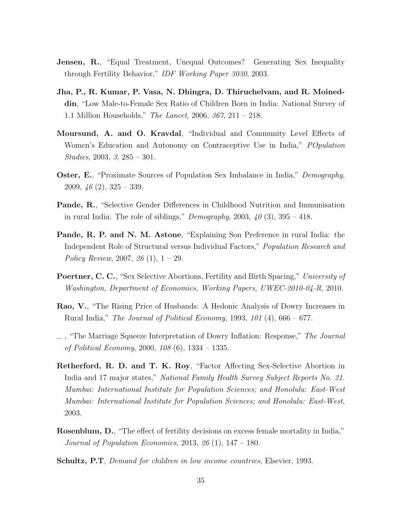
Jensen, R., “Equal Treatment, Unequal Outcomes? Generating Sex Inequality

through Fertility Behavior,” IDF Working Paper 3030, 2003.

Jha, P., R. Kumar, P. Vasa, N. Dhingra, D. Thiruchelvam, and R. Moined-

din, “Low Male-to-Female Sex Ratio of Children Born in India: National Survey of

1.1 Million Households,” The Lancet, 2006, 367, 211 – 218.

Moursund, A. and O. Kravdal, “Individual and Community Level E↵ects of

Women’s Education and Autonomy on Contraceptive Use in India,” POpulation

Studies, 2003, 3, 285 – 301.

Oster, E., “Proximate Sources of Population Sex Imbalance in India,” Demography,

2009, 46 (2), 325 – 339.

Pande, R., “Selective Gender Di↵erences in Childhood Nutrition and Immunisation

in rural India: The role of siblings,” Demography, 2003, 40 (3), 395 – 418.

Pande, R. P. and N. M. Astone, “Explaining Son Preference in rural India: the

Independent Role of Structural versus Individual Factors,” Population Research and

Policy Review, 2007, 26 (1), 1 – 29.

Poertner, C. C., “Sex Selective Abortions, Fertility and Birth Spacing,” University of

Washington, Department of Economics, Working Papers, UWEC-2010-04-R, 2010.

Rao, V., “The Rising Price of Husbands: A Hedonic Analysis of Dowry Increases in

Rural India,” The Journal of Political Economy, 1993, 101 (4), 666 – 677.

, “The Marriage Squeeze Interpretation of Dowry Inflation: Response,” The Journal

of Political Economy, 2000, 108 (6), 1334 – 1335.

Retherford, R. D. and T. K. Roy, “Factor A↵ecting Sex-Selective Abortion in

India and 17 major states,” National Family Health Survey Subject Reports No. 21.

Mumbai: International Institute for Population Sciences; and Honolulu: East-West

Mumbai: International Institute for Population Sciences; and Honolulu: East-West,

2003.

Rosenblum, D., “The e↵ect of fertility decisions on excess female mortality in India,”

Journal of Population Economics, 2013, 26 (1), 147 – 180.

Schultz, P.T, Demand for children in low income countries, Elsevier, 1993.

35

Smith, Herbert L., Sharon J. Ghuman, Sharon J. Lee, and Karen Oppen-

heim Mason, “Status of Women and Fertility,” Machine-readable data file, 2000.

Srinivas, M. N., Oxford University Press, India, 1997.

Srinivasan, T. N., “Sex preferences, stopping rules and fertility,” Yale University

Working Papers, New Haven, CT, 1992.

Tertilt, Michele, “Polygyny, Fertility, and Savings,” Journal of Political Economy,

2005, 113 (6), 1341 – 1371.

United Nations, Department of Economic and Social A↵airs, Population

Division, ESA/P/WP.227, 2013.

United Nations Development Programme, Palgrave Mamillan, 2006.

Wang, W. and F. Famoye, “Modeling Household Fertility Decisions with General-

ized Poisson Regression,” Population Economics, 1997, 10, 273 – 283.

Yamaguchi, K., “A Formal Theory for Male-Preferring Stopping Rules of Childbear-

ing: Sex Di↵erences in Birth Order and in the Number of Siblings,” Demography,

1989, 26, 451 – 65.

Yount, K. M., R. Laangsten, and K. Hill, “The E↵ect of Gender Preference on

Contraceptive Use in Fertility in Rural Egypt,” Studies in Family Planning, 2000,

31 (4), 290 – 300.

36

Figures

Figure 1: Mean Number of Births Per Woman

01

23

45

Num

ber o

f boy

s an

d gi

rls

0.0

5.1

.15

.2Fr

actio

n of

tota

l birt

hs

0 2 4 6 8 10Total Births

Fraction Sons bornGirls born

Notes: Sample consists of women born between 1942 and 1970, aged 36 to 49 years at interview anddrawn from NFHS-1, NFHS-2 and NFHS-3; own calculations.

Figure 2: Ideal Number of Children, Boys and Girls

01

23

4

1940 1950 1960 1970Mother's Year of Birth

Children BoysGirls Boys minus Girls

Notes: Sample consists of women born between 1942 and 1970, aged 36 to 49 years at interview anddrawn from NFHS-1, NFHS-2 and NFHS-3; own calculations.

37

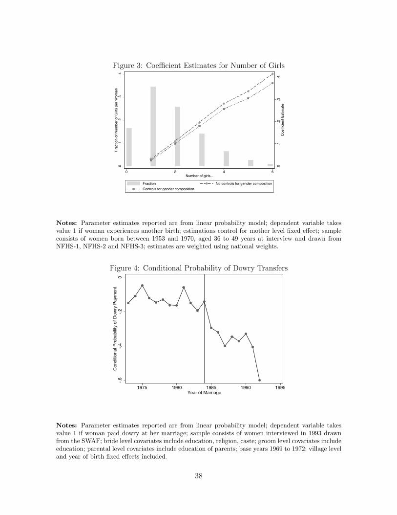
Figure 3: Coe�cient Estimates for Number of Girls

0.1

.2.3

.4C

oeffi

cien

t Est

imat

e

0.1

.2.3

.4Fr

actio

n of

Num

ber o

f Girl

s pe

r Wom

an

0 2 4 6Number of girls...

Fraction No controls for gender compositionControls for gender composition

Notes: Parameter estimates reported are from linear probability model; dependent variable takesvalue 1 if woman experiences another birth; estimations control for mother level fixed e↵ect; sampleconsists of women born between 1953 and 1970, aged 36 to 49 years at interview and drawn fromNFHS-1, NFHS-2 and NFHS-3; estimates are weighted using national weights.

Figure 4: Conditional Probability of Dowry Transfers

-.6-.4

-.20

Con

ditio

nal P

roba

bilit

y of

Dow

ry P

aym

ent

1975 1980 1985 1990 1995Year of Marriage

Notes: Parameter estimates reported are from linear probability model; dependent variable takesvalue 1 if woman paid dowry at her marriage; sample consists of women interviewed in 1993 drawnfrom the SWAF; bride level covariates include education, religion, caste; groom level covariates includeeducation; parental level covariates include education of parents; base years 1969 to 1972; village leveland year of birth fixed e↵ects included.

38

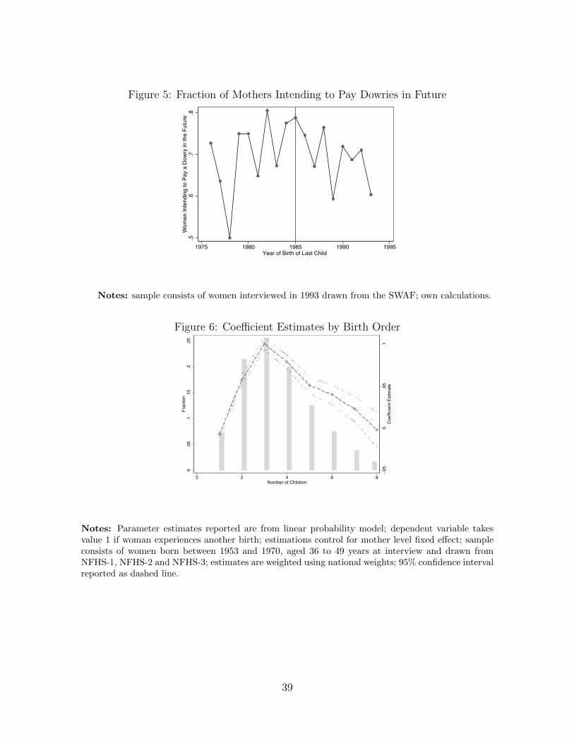
Figure 5: Fraction of Mothers Intending to Pay Dowries in Future

.5.6

.7.8

Wom

en In

tend

ing

to P

ay a

Dow

ry in

the

Futu

re

1975 1980 1985 1990 1995Year of Birth of Last Child

Notes: sample consists of women interviewed in 1993 drawn from the SWAF; own calculations.

Figure 6: Coe�cient Estimates by Birth Order

-.05

0.0

5.1

Coe

ffici

ent E

stim

ate

0.0

5.1

.15

.2.2

5Fr

actio

n

0 2 4 6 8Number of Children

Notes: Parameter estimates reported are from linear probability model; dependent variable takesvalue 1 if woman experiences another birth; estimations control for mother level fixed e↵ect; sampleconsists of women born between 1953 and 1970, aged 36 to 49 years at interview and drawn fromNFHS-1, NFHS-2 and NFHS-3; estimates are weighted using national weights; 95% confidence intervalreported as dashed line.

39

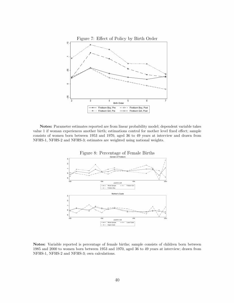
Figure 7: E↵ect of Policy by Birth Order

-.05

0.0

5.1

.15

2 3 4 5 6 7Birth Order

Firstborn Boy, Pre Firstborn Boy, PostFirstborn Girl, Pre Firstborn Girl, Post

Notes: Parameter estimates reported are from linear probability model; dependent variable takesvalue 1 if woman experiences another birth; estimations control for mother level fixed e↵ect; sampleconsists of women born between 1953 and 1970, aged 36 to 49 years at interview and drawn fromNFHS-1, NFHS-2 and NFHS-3; estimates are weighted using national weights.

Figure 8: Percentage of Female Births

.46

.48

.5.5

2.5

4

1985 1990 1995 2000yearbirth_kid2

Whole Sample Firstborn Girl

Firstborn Boy

Gender of Firstborn

.46

.48

.5.5

2.5

4

1985 1990 1995 2000yearbirth_kid2

Whole Sample Lower Caste

Higher Caste

Mother's Caste

Notes: Variable reported is percentage of female births; sample consists of children born between1985 and 2000 to women born between 1953 and 1970, aged 36 to 49 years at interview; drawn fromNFHS-1, NFHS-2 and NFHS-3; own calculations.

40

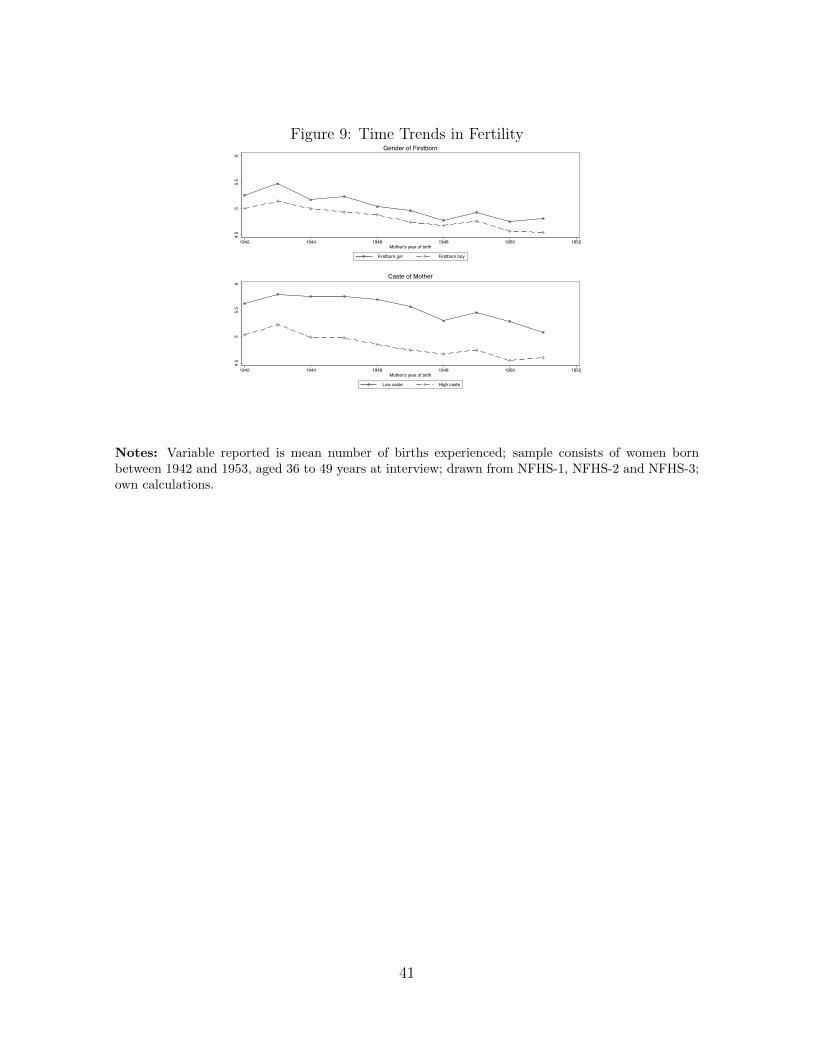
Figure 9: Time Trends in Fertility

4.5

55.

56

1942 1944 1946 1948 1950 1952Mother's year of birth

Firstborn girl Firstborn boy

Gender of Firstborn

4.5

55.

56

1942 1944 1946 1948 1950 1952Mother's year of birth

Low caste High caste

Caste of Mother

Notes: Variable reported is mean number of births experienced; sample consists of women bornbetween 1942 and 1953, aged 36 to 49 years at interview; drawn from NFHS-1, NFHS-2 and NFHS-3;own calculations.

41

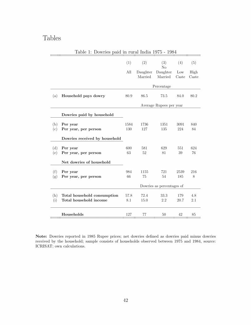
Tables

Table 1: Dowries paid in rural India 1975 - 1984

(1) (2) (3) (4) (5)No

All Daughter Daughter Low HighMarried Married Caste Caste

Percentage

(a) Household pays dowry 80.9 86.5 73.5 84.0 80.2

Average Rupees per year

Dowries paid by household

(b) Per year 1584 1736 1351 3091 840(c) Per year, per person 130 127 135 224 84

Dowries received by household

(d) Per year 600 581 629 551 624(e) Per year, per person 63 52 81 39 76

Net dowries of household

(f) Per year 984 1155 721 2539 216(g) Per year, per person 66 75 54 185 8

Dowries as percentages of

(h) Total household consumption 57.8 72.4 33.3 179 4.8(i) Total household income 8.1 15.0 2.2 20.7 2.1

Households 127 77 50 42 85

Note: Dowries reported in 1985 Rupee prices; net dowries defined as dowries paid minus dowriesreceived by the household; sample consists of households observed between 1975 and 1984, source:ICRISAT; own calculations.

42

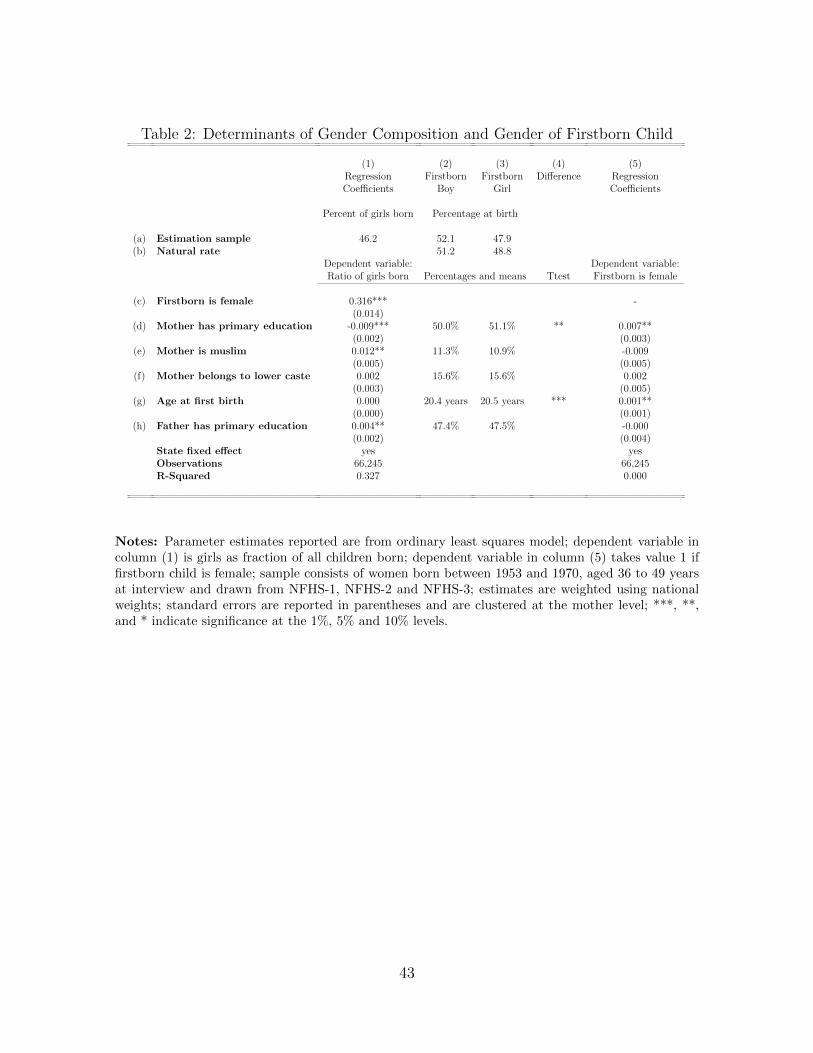
Table 2: Determinants of Gender Composition and Gender of Firstborn Child

(1) (2) (3) (4) (5)Regression Firstborn Firstborn Di↵erence RegressionCoe�cients Boy Girl Coe�cients

Percent of girls born Percentage at birth

(a) Estimation sample 46.2 52.1 47.9(b) Natural rate 51.2 48.8

Dependent variable: Dependent variable:Ratio of girls born Percentages and means Ttest Firstborn is female

(c) Firstborn is female 0.316*** -(0.014)

(d) Mother has primary education -0.009*** 50.0% 51.1% ** 0.007**(0.002) (0.003)

(e) Mother is muslim 0.012** 11.3% 10.9% -0.009(0.005) (0.005)

(f) Mother belongs to lower caste 0.002 15.6% 15.6% 0.002(0.003) (0.005)

(g) Age at first birth 0.000 20.4 years 20.5 years *** 0.001**(0.000) (0.001)

(h) Father has primary education 0.004** 47.4% 47.5% -0.000(0.002) (0.004)

State fixed e↵ect yes yesObservations 66,245 66,245R-Squared 0.327 0.000

Notes: Parameter estimates reported are from ordinary least squares model; dependent variable incolumn (1) is girls as fraction of all children born; dependent variable in column (5) takes value 1 iffirstborn child is female; sample consists of women born between 1953 and 1970, aged 36 to 49 yearsat interview and drawn from NFHS-1, NFHS-2 and NFHS-3; estimates are weighted using nationalweights; standard errors are reported in parentheses and are clustered at the mother level; ***, **,and * indicate significance at the 1%, 5% and 10% levels.

43

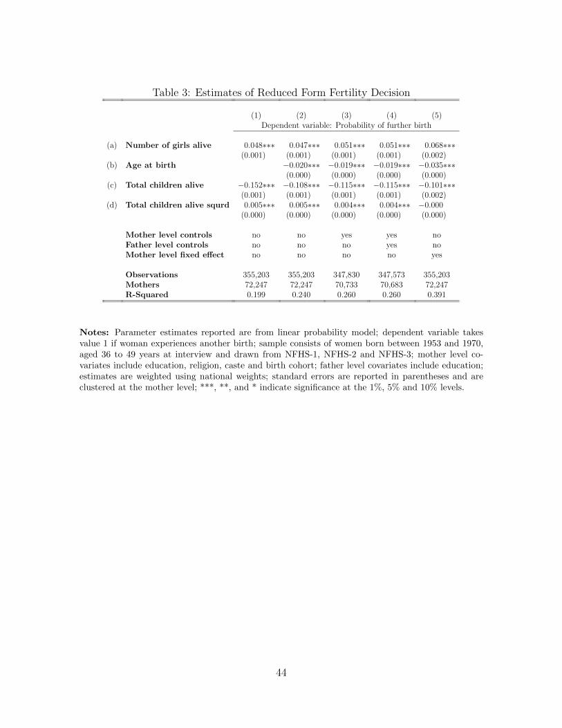
Table 3: Estimates of Reduced Form Fertility Decision

(1) (2) (3) (4) (5)Dependent variable: Probability of further birth

(a) Number of girls alive 0.048⇤⇤⇤ 0.047⇤⇤⇤ 0.051⇤⇤⇤ 0.051⇤⇤⇤ 0.068⇤⇤⇤(0.001) (0.001) (0.001) (0.001) (0.002)

(b) Age at birth �0.020⇤⇤⇤ �0.019⇤⇤⇤ �0.019⇤⇤⇤ �0.035⇤⇤⇤(0.000) (0.000) (0.000) (0.000)

(c) Total children alive �0.152⇤⇤⇤ �0.108⇤⇤⇤ �0.115⇤⇤⇤ �0.115⇤⇤⇤ �0.101⇤⇤⇤(0.001) (0.001) (0.001) (0.001) (0.002)

(d) Total children alive squrd 0.005⇤⇤⇤ 0.005⇤⇤⇤ 0.004⇤⇤⇤ 0.004⇤⇤⇤ �0.000(0.000) (0.000) (0.000) (0.000) (0.000)

Mother level controls no no yes yes noFather level controls no no no yes noMother level fixed e↵ect no no no no yes

Observations 355,203 355,203 347,830 347,573 355,203Mothers 72,247 72,247 70,733 70,683 72,247R-Squared 0.199 0.240 0.260 0.260 0.391

Notes: Parameter estimates reported are from linear probability model; dependent variable takesvalue 1 if woman experiences another birth; sample consists of women born between 1953 and 1970,aged 36 to 49 years at interview and drawn from NFHS-1, NFHS-2 and NFHS-3; mother level co-variates include education, religion, caste and birth cohort; father level covariates include education;estimates are weighted using national weights; standard errors are reported in parentheses and areclustered at the mother level; ***, **, and * indicate significance at the 1%, 5% and 10% levels.

44

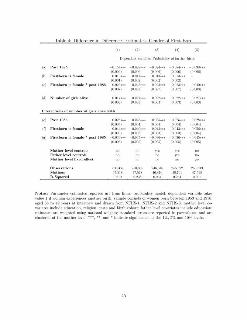
Table 4: Di↵erence in Di↵erences Estimates: Gender of First Born

(1) (2) (3) (4) (5)

Dependent variable: Probability of further birth

(a) Post 1985 �0.154⇤⇤⇤ �0.088⇤⇤⇤ �0.084⇤⇤⇤ �0.084⇤⇤⇤ �0.098⇤⇤⇤(0.006) (0.006) (0.006) (0.006) (0.006)

(b) Firstborn is female 0.010⇤⇤⇤ 0.011⇤⇤⇤ 0.013⇤⇤⇤ 0.013⇤⇤⇤ �(0.001) (0.002) (0.002) (0.002)

(c) Firstborn is female * post 1985 0.026⇤⇤⇤ 0.025⇤⇤⇤ 0.023⇤⇤⇤ 0.023⇤⇤⇤ 0.040⇤⇤⇤(0.007) (0.007) (0.007) (0.007) (0.008)

(d) Number of girls alive 0.017⇤⇤⇤ 0.021⇤⇤⇤ 0.022⇤⇤⇤ 0.022⇤⇤⇤ 0.027⇤⇤⇤(0.003) (0.003) (0.003) (0.003) (0.003)

Interactions of number of girls alive with

(e) Post 1985 0.028⇤⇤⇤ 0.025⇤⇤⇤ 0.025⇤⇤⇤ 0.025⇤⇤⇤ 0.028⇤⇤⇤(0.004) (0.004) (0.004) (0.004) (0.004)

(f) Firstborn is female 0.044⇤⇤⇤ 0.040⇤⇤⇤ 0.043⇤⇤⇤ 0.043⇤⇤⇤ 0.056⇤⇤⇤(0.003) (0.003) (0.003) (0.003) (0.004)

(g) Firstborn is female * post 1985 �0.039⇤⇤⇤ �0.037⇤⇤⇤ �0.036⇤⇤⇤ �0.036⇤⇤⇤ �0.045⇤⇤⇤(0.005) (0.005) (0.005) (0.005) (0.005)

Mother level controls no no yes yes noFather level controls no no no yes noMother level fixed e↵ect no no no no yes

Observations 250,339 250,339 246,346 246,092 250,339Mothers 47,518 47,518 46,810 46,761 47,518R-Squared 0.219 0.238 0.254 0.254 0.391

Notes: Parameter estimates reported are from linear probability model; dependent variable takesvalue 1 if woman experiences another birth; sample consists of women born between 1953 and 1970,aged 36 to 49 years at interview and drawn from NFHS-1, NFHS-2 and NFHS-3; mother level co-variates include education, religion, caste and birth cohort; father level covariates include education;estimates are weighted using national weights; standard errors are reported in parentheses and areclustered at the mother level; ***, **, and * indicate significance at the 1%, 5% and 10% levels.

45

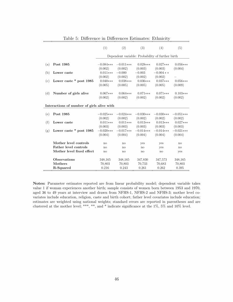
Table 5: Di↵erence in Di↵erences Estimates: Ethnicity

(1) (2) (3) (4) (5)

Dependent variable: Probability of further birth

(a) Post 1985 �0.084⇤⇤⇤ �0.011⇤⇤⇤ 0.028⇤⇤⇤ 0.027⇤⇤⇤ 0.056⇤⇤⇤(0.002) (0.002) (0.003) (0.003) (0.004)

(b) Lower caste 0.011⇤⇤⇤ �0.000 �0.003 �0.004 ⇤ ⇤(0.002) (0.002) (0.002) (0.002) �

(c) Lower caste * post 1985 0.040⇤⇤⇤ 0.038⇤⇤⇤ 0.036⇤⇤⇤ 0.037⇤⇤⇤ 0.056⇤⇤⇤(0.005) (0.005) (0.005) (0.005) (0.009)

(d) Number of girls alive 0.067⇤⇤⇤ 0.064⇤⇤⇤ 0.071⇤⇤⇤ 0.071⇤⇤⇤ 0.103⇤⇤⇤(0.002) (0.002) (0.002) (0.002) (0.002)

Interactions of number of girls alive with

(e) Post 1985 �0.025⇤⇤⇤ �0.024⇤⇤⇤ �0.030⇤⇤⇤ �0.030⇤⇤⇤ �0.051⇤⇤⇤(0.002) (0.002) (0.002) (0.002) (0.002)

(f) Lower caste 0.011⇤⇤⇤ 0.011⇤⇤⇤ 0.013⇤⇤⇤ 0.013⇤⇤⇤ 0.027⇤⇤⇤(0.003) (0.003) (0.003) (0.003) (0.003)

(g) Lower caste * post 1985 �0.020⇤⇤⇤ �0.017⇤⇤⇤ �0.014⇤⇤⇤ �0.014⇤⇤⇤ �0.021⇤⇤⇤(0.004) (0.004) (0.004) (0.004) (0.004)

Mother level controls no no yes yes noFather level controls no no no yes noMother level fixed e↵ect no no no no yes

Observations 348,165 348,165 347,830 347,573 348,165Mothers 70,803 70,803 70,733 70,683 70,803R-Squared 0.216 0.243 0.261 0.262 0.395

Notes: Parameter estimates reported are from linear probability model; dependent variable takesvalue 1 if woman experiences another birth; sample consists of women born between 1953 and 1970,aged 36 to 49 years at interview and drawn from NFHS-1, NFHS-2 and NFHS-3; mother level co-variates include education, religion, caste and birth cohort; father level covariates include education;estimates are weighted using national weights; standard errors are reported in parentheses and areclustered at the mother level; ***, **, and * indicate significance at the 1%, 5% and 10% level.

46

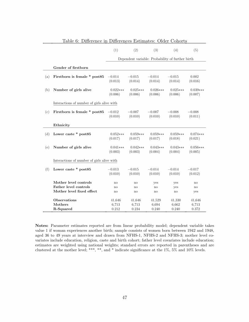
Table 6: Di↵erence in Di↵erences Estimates: Older Cohorts

(1) (2) (3) (4) (5)

Dependent variable: Probability of further birth

Gender of firstborn

(a) Firstborn is female * post85 �0.014 �0.015 �0.014 �0.015 0.002(0.013) (0.014) (0.014) (0.014) (0.016)

(b) Number of girls alive 0.022⇤⇤⇤ 0.025⇤⇤⇤ 0.026⇤⇤⇤ 0.025⇤⇤⇤ 0.039⇤⇤⇤(0.006) (0.006) (0.006) (0.006) (0.007)

Interactions of number of girls alive with

(c) Firstborn is female * post85 �0.012 �0.007 �0.007 �0.008 �0.008(0.010) (0.010) (0.010) (0.010) (0.011)

Ethnicity

(d) Lower caste * post85 0.052⇤⇤⇤ 0.059⇤⇤⇤ 0.059⇤⇤⇤ 0.059⇤⇤⇤ 0.074⇤⇤⇤(0.017) (0.017) (0.017) (0.018) (0.021)

(e) Number of girls alive 0.041⇤⇤⇤ 0.042⇤⇤⇤ 0.043⇤⇤⇤ 0.043⇤⇤⇤ 0.056⇤⇤⇤(0.003) (0.003) (0.004) (0.004) (0.005)

Interactions of number of girls alive with

(f) Lower caste * post85 �0.013 �0.015 �0.014 �0.014 �0.017(0.010) (0.010) (0.010) (0.010) (0.012)

Mother level controls no no yes yes noFather level controls no no no yes noMother level fixed e↵ect no no no no yes

Observations 41,646 41,646 41,529 41,330 41,646Mothers 6,713 6,713 6,694 6,662 6,713R-Squared 0.212 0.234 0.240 0.240 0.372

Notes: Parameter estimates reported are from linear probability model; dependent variable takesvalue 1 if woman experiences another birth; sample consists of women born between 1942 and 1948,aged 36 to 49 years at interview and drawn from NFHS-1, NFHS-2 and NFHS-3; mother level co-variates include education, religion, caste and birth cohort; father level covariates include education;estimates are weighted using national weights; standard errors are reported in parentheses and areclustered at the mother level; ***, **, and * indicate significance at the 1%, 5% and 10% levels.

47

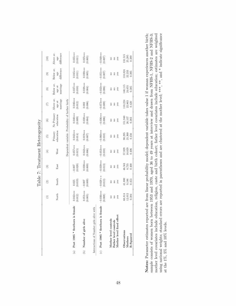
Tab

le7:

TreatmentHeterogeneity

(1)

(2)

(3)

(4)

(5)

(6)

(7)

(8)

(9)

(10)

Primary

NoPrimary

Aboveav.

Below

av.

Below

av.

Aboveav.

North

Sou

thEast

West

education

education

ageat

ageat

age

age

marriage

marriage

di↵erence

di↵erence

Dep

endentvariab

le:Probab

ilityof

further

birth

(a)

Post

1985*firstb

orn

isfemale

0.042⇤⇤⇤

0.025

�0.007

0.057⇤⇤⇤

0.042⇤⇤⇤

0.040⇤⇤⇤

0.046⇤⇤⇤

0.037⇤⇤⇤

0.045⇤⇤⇤

0.035⇤⇤⇤

(0.012)

(0.019)

(0.020)

(0.015)

(0.014)

(0.009)

(0.012)

(0.010)

(0.011)

(0.011)

(b)

Number

ofgirls

alive

0.051⇤⇤⇤

�0.007

0.030⇤⇤⇤

0.042⇤⇤⇤

0.019⇤⇤⇤

0.038⇤⇤⇤

0.002

0.038⇤⇤⇤

0.030⇤⇤⇤

0.025⇤⇤⇤

(0.005)

(0.009)

(0.009)

(0.006)

(0.007)

(0.004)

(0.006)

(0.004)

(0.005)

(0.005)

Interactionsof

Number

girlsalivewith

(c)

Post

1985*firstb

orn

isfemale

�0.036⇤⇤⇤

�0.029⇤⇤

�0.039⇤⇤⇤

�0.053⇤⇤⇤

�0.060⇤⇤⇤

�0.036⇤⇤⇤

�0.073⇤⇤⇤

�0.033⇤⇤⇤

�0.051⇤⇤⇤

�0.040⇤⇤⇤

(0.008)

(0.013)

(0.013)

(0.010)

(0.010)

(0.006)

(0.009)

(0.006)

(0.007)

(0.007)

Moth

erlevel

controls

no

no

no

no

no

no

no

no

no

no

Fath

erlevel

controls

no

no

no

no

no

no

no

no

no

no

Moth

erlevel

fixed

e↵ec

tyes

yes

yes

yes

yes

yes

yes

yes

yes

yes

Observations

68,814

41,880

46,561

57,929

98,295

151,940

110,224

140,115

118,824

131,515

Moth

ers

12,012

9,186

8,735

10,829

21,360

26,137

22,863

24,655

22,233

25,285

R-S

quared

0.384

0.453

0.400

0.406

0.456

0.383

0.420

0.385

0.395

0.389

Notes:Param

eter

estimates

reportedarefrom

linearprobab

ilitymod

el;dep

endentvariab

letakesvalue1ifwom

anexperiencesan

other

birth;

sample

consistsof

wom

enbornbetween1953

and1970,aged

36to

49yearsat

interview

anddrawnfrom

NFHS-1,NFHS-2

andNFHS-3;

mother

levelcovariates

includeeducation

,religion

,castean

dbirth

cohort;

father

levelcovariates

includeeducation

;estimates

areweigh

ted

usingnational

weigh

ts;stan

darderrors

arereportedin

parentheses

andareclustered

atthemother

level;***,

**,an

d*indicatesign

ificance

atthe1%

,5%

and10%

levels.

48

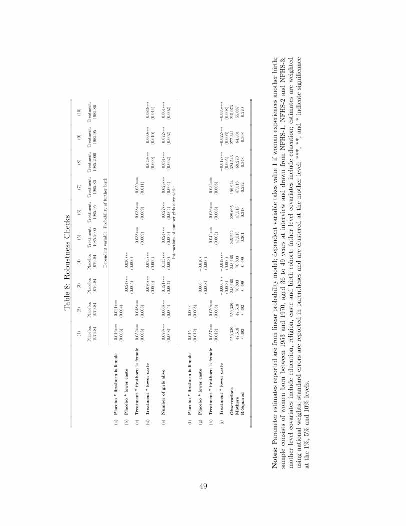
Tab

le8:

Rob

ustnessChecks

(1)

(2)

(3)

(4)

(5)

(6)

(7)

(8)

(9)

(10)

Placebo:

Placebo:

Placebo:

Placebo:

Treatment:

Treatment:

Treatment:

Treatment:

Treatment:

Treatment:

1976-84

1979-84

1976-84

1979-84

1985-2000

1985-95

1985-86

1985-2000

1985-95

1985-86

Dep

endentvariab

le:Probab

ilityof

further

birth

(a)

Place

bo*firstb

orn

isfemale

0.016⇤⇤⇤

0.021⇤⇤⇤

(0.003)

(0.004)

(b)

Place

bo*lower

caste

0.024⇤⇤⇤

0.036⇤⇤⇤

(0.005)

(0.006)

(c)

Treatm

ent*firstb

orn

isfemale

0.052⇤⇤⇤

0.048⇤⇤⇤

0.038⇤⇤⇤

0.038⇤⇤⇤

0.050⇤⇤⇤

(0.008)

(0.008)

(0.009)

(0.009)

(0.011)

(d)

Treatm

ent*lower

caste

0.070⇤⇤⇤

0.073⇤⇤⇤

0.049⇤⇤⇤

0.060⇤⇤⇤

0.083⇤⇤⇤

(0.009)

(0.009)

(0.009)

(0.010)

(0.014)

(e)

Number

ofgirls

alive

0.079⇤⇤⇤

0.066⇤⇤⇤

0.121⇤⇤⇤

0.133⇤⇤⇤

0.024⇤⇤⇤

0.022⇤⇤⇤

0.028⇤⇤⇤

0.091⇤⇤⇤

0.072⇤⇤⇤

0.061⇤⇤⇤

(0.008)

(0.005)

(0.004)

(0.003)

(0.003)

(0.004)

(0.004)

(0.002)

(0.002)

(0.002)

Interactionsof

number

girlsalivewith:

(f)

Place

bo*firstb

orn

isfemale

�0.015

�0.009

(0.012)

(0.008)

(g)

Place

bo*lower

caste

0.006

�0.010⇤

(0.008)

(0.006)

(h)

Treatm

ent*firstb

orn

isfemale

�0.057⇤⇤⇤

�0.050⇤⇤⇤

�0.042⇤⇤⇤

�0.036⇤⇤⇤

�0.032⇤⇤⇤

(0.012)

(0.008)

(0.005)

(0.006)

(0.008)

(i)

Treatm

ent*lower

caste

�0.006⇤⇤

�0.018⇤⇤⇤

�0.017⇤⇤⇤

�0.022⇤⇤⇤

�0.035⇤⇤⇤

(0.003)

(0.006)

(0.005)

(0.006)

(0.008)

Observations

250,339

250,339

348,165

348,165

245,222

228,695

198,924

324,543

277,341

215,073

Moth

ers

47,518

47,518

70,803

70,803

47,518

47,518

47,518

69,270

64,504

55,087

R-S

quared

0.392

0.392

0.399

0.399

0.361

0.318

0.272

0.348

0.308

0.270

Notes:Param

eter

estimates

reportedarefrom

linearprobab

ilitymod

el;dep

endentvariab

letakesvalue1ifwom

anexperiencesan

other

birth;

sample

consistsof

wom

enbornbetween1953

and1970,aged

36to

49yearsat

interview

anddrawnfrom

NFHS-1,NFHS-2

andNFHS-3;

mother

levelcovariates

includeeducation

,religion

,castean

dbirth

cohort;

father

levelcovariates

includeeducation

;estimates

areweigh

ted

usingnational

weigh

ts;stan

darderrors

arereportedin

parentheses

andareclustered

atthemother

level;***,

**,an

d*indicatesign

ificance

atthe1%

,5%

and10%

levels.

49