Dates of the Two Most Recent Surface Ruptures on the Southernmost

San Andreas Fault Recalculated by Precise Dating

of Lake Cahuilla Dry Periods

by Thomas K. Rockwell, Aron J. Meltzner,* and Erik C. Haaker

Abstract The past two southernmost San Andreas fault (SAF) ruptures occurredwhen ancient Lake Cahuilla was full, based on faulted lake sediment relationships andextensive liquefaction at sites near the shoreline. The times of the past two southernSAF ruptures have been reevaluated with new radiocarbon data on in situ stumps thatgrew between the past three Lake Cahuilla highstands, which, when taken in combi-nation with historical accounts and modeling of the time to fill and desiccate the lake,provide more precise and accurate ages for the past two SAF earthquakes. The 14Cdates on inner and outer rings combined with historical observations show that the dryperiod prior to the last lake ended after 1706 C.E., leaving a narrow window of lessthan 25 yrs to fill and begin desiccating the most recent lake, and that the penultimatelake began dropping from a highstand around 1640 C.E. or earlier. Our analysis showsthat the most recent earthquake occurred about 1726� 7 C.E., whereas the timing ofthe penultimate event is slightly older at 1577� 67 C.E. (both at 2σ). These newdates, when combined with previous age estimates of earlier southern SAF events,suggest more regular recurrence of surface-rupturing events, with an average intervalof about 180 yrs, but leave the open interval at nearly 300 yrs.

Introduction

Assessment of earthquake hazard from fast-moving faultsusing time-dependent forecast models is critically dependenton knowing the timing of the most recent large earthquake(Gomberg et al., 2005; Petersen et al., 2007; Field et al.,2015). This is particularly true for the southern San Andreasfault (SAF), where the published average recurrence intervalfor the past millennium is on the order of 116–221 yrs, with abest estimate of 180 yrs (Philibosian et al., 2011), whereas thelast large surface rupture has been estimated to have occurred330–340 yrs ago (Sieh, 1986; Sieh andWilliams, 1990; Fumalet al., 2002; Philibosian et al., 2011). All of these studies usedradiocarbon dating to resolve the timing of past earthquakes,but the radiocarbon calibration curve for the time period afterabout 1680 C.E. fluctuates about a horizontal axis, resulting inmultiple age intercepts and discrete, broad ranges for predictedearthquake ages. The historical record has been used to trimthese dates, but the historical observations are sparse, allowingfor substantial uncertainty in the timing of the most recentlarge southern SAF earthquake.

The southern SAF crosses the shoreline and lake depos-its of ancient Lake Cahuilla (Fig. 1), a freshwater lake that

covered much of the Salton trough, up to its sill elevation of13 m above sea level, at least six times in the past 1000–1200yrs (Waters, 1983; Gurrola and Rockwell, 1996; Philibosianet al., 2011). The two most recent southern SAF surface rup-tures are interpreted to have occurred during the two mostrecent highstands of Lake Cahuilla, based on the presence ofextensive liquefaction, plastic slumping, and soft-sedimentdeformation of lake deposits in association with upwardtermination of fault splays and accumulation of growth strata(Sieh, 1986; Sieh and Williams, 1990; Philibosian et al.,2011).

The timings of these past earthquakes are based, in part,on radiocarbon dates on detrital charcoal recovered from thelake sediments. Because wood in this region neither growsunder water nor burns in the water, most of the detrital char-coal is either derived from outside the lake basin or repre-sents wood growth below the lake shoreline during a dryperiod between lakes. Consequently, the published datesof large SAF earthquakes almost certainly are older thanthe actual dates of the events because they do not accountfor the inherited age of the wood, which includes the timebetween plant growth and death, the burning of the wood,and the transport and burial of the charcoal in the lakesediments.

*Also at Asian School of the Environment, Nanyang TechnologicalUniversity, 50 Nanyang Avenue, Singapore 639798, Singapore.

BSSA Early Edition / 1

Bulletin of the Seismological Society of America, Vol. XX, No. XX, pp. –, – 2018, doi: 10.1785/0120170392

To better date the past two southern SAF earthquakes,we apply a new approach to date the lake sediments that dis-play evidence of faulting. We dated the dry interval betweenthe past two lake highstands by collecting several dead mes-quite stumps that were inundated by the most recent lake(lake A), and we add dates from one stump (SB 3DIII-23;Orgil, 2001) from below the penultimate lake (lake B). Wealso add radiocarbon ages obtained on two particularlyyoung detrital charcoal samples associated with the fillingof lake B and inferred to be derived from wood that grewand burned during the preceding dry period, between lakesB and C. The first sample (C25b/P3; Gurrola and Rockwell,1996) was extracted from a shoreline peat-like organic layer,whereas the second (IFD-T2-C67; Rockwell et al., 2011)was embedded within the penultimate lake-filling sequenceat a site at −32 m elevation. These new data place tight con-straints on when there was no water at various elevationswithin the basin. Finally, we add radiocarbon ages fromyoung detrital charcoal samples embedded within the lakeB deposits at a site at the shoreline (Philibosian et al.,2011); these samples provide a maximum age on when lakeB began to recede. We then combine these data with model-ing of the time required to completely fill and desiccate a lakebased on reasonable rates of discharge from the ColoradoRiver and estimates of local and regional desiccation ratesthat we combine with the historical observations to more

precisely date the most recent two lakestands that together improve both theaccuracy and precision of the ages ofthe two most recent large southern SAFearthquakes.

Collection and Dating of In SituStumps

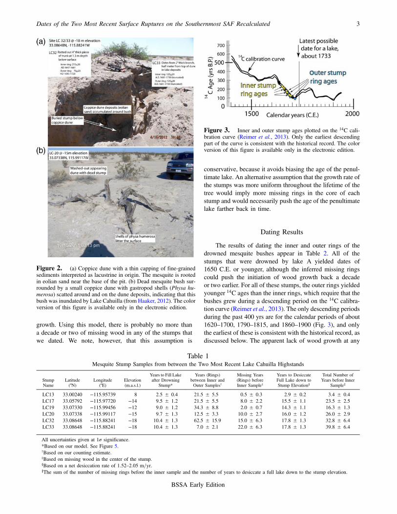
Stumps of dead mesquite (Prosopissp., probably P. glandulosa) that were in-undated by the most recent highstand ofLake Cahuilla are recognized in two ways.Some are now buried by lacustrine sedi-ments, and we exposed them in trenches orby hand digging around the remnant topsof the bushes to expose the entire buriedbush (Fig. 2a) (Haaker, 2012). More com-monly, stumps were found in areas of littleor no sedimentation from the last lake andexhibited coppice dunes around theirbases. The coppice dunes appear to havebeen washed by water and are coveredin gastropod shells (Physa humerosa;Fig. 2b).

In each case, we collected the entirestump by sawing it from its base, and wecut cross sections though it is in the lab.From the cross section with the most com-

plete set of rings, we sampled the innermost and outermost2–3 rings for radiocarbon dating. The wood samples werepretreated with the standard acid–base–acid rinses and datedat the Center for Accelerator Mass Spectrometry facility atUniversity of California Irvine. For our age model, we as-sumed the growth rings were annual, and we counted thenumber of rings between the samples to provide an estimateof the expected number of years between the paired dates,allowing for reasonable uncertainties (Table 1).

In most cases, the core of the stump had been eaten awayby termites, so the older part of the age range for thesestumps is missing. We attempt to account for this by estimat-ing the number of missing rings based on how much of thecore is gone (Table 1). For the missing core of each stump,we used the documented growth rate of P. glandulosa foryoung trees with ample water supply of 4 cm/decade (Ansleyet al., 2010). We assumed that the initial growth of the mes-quite likely initiated with the drawdown of Lake Cahuillaand that the mesquite taproot could keep up with the draw-down, initially maintaining rapid growth, although the mes-quite could have started growing at any time after recession,which we also account for in our model. We hypothesize thatthe reason that most of the mesquite samples we collectedhad the heartwood eaten by termites is that the initial woodgrowth was from the early period of rapid growth and waslikely softer than the outer rings, as is common in trees thatformed after the water table dropped sufficiently to slow

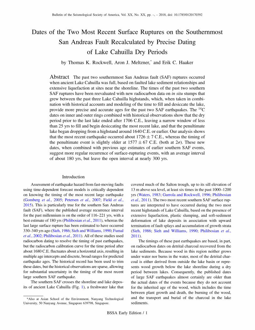
Figure 1. Map of the southern San Andreas fault (SAF) system showing paleoseis-mic sites (stars) on the SAF above, at, and below the shoreline of Lake Cahuilla that isshown at �13 m elevation. The color version of this figure is available only in the elec-tronic edition.

2 T. K. Rockwell, A. J. Meltzner, and E. C. Haaker

BSSA Early Edition

growth. Using this model, there is probably no more thana decade or two of missing wood in any of the stumps thatwe dated. We note, however, that this assumption is

conservative, because it avoids biasing the age of the penul-timate lake. An alternative assumption that the growth rate ofthe stumps was more uniform throughout the lifetime of thetree would imply more missing rings in the core of eachstump and would necessarily push the age of the penultimatelake farther back in time.

Dating Results

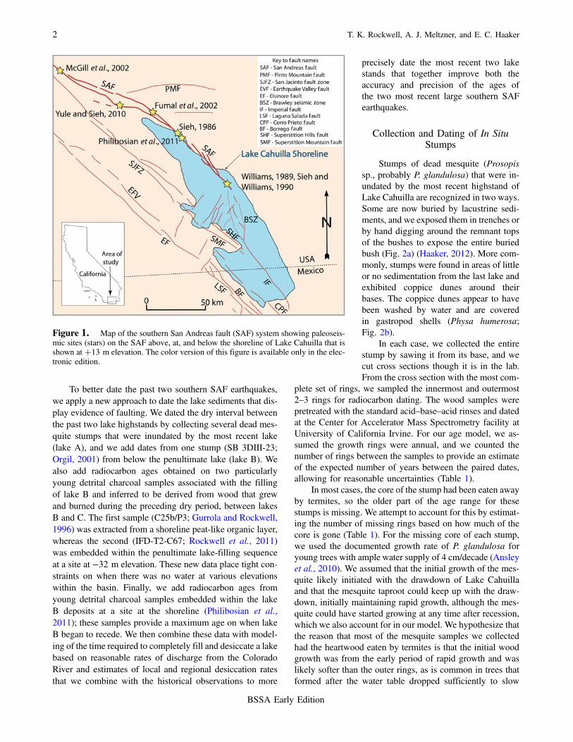
The results of dating the inner and outer rings of thedrowned mesquite bushes appear in Table 2. All of thestumps that were drowned by lake A yielded dates of1650 C.E. or younger, although the inferred missing ringscould push the initiation of wood growth back a decadeor two earlier. For all of these stumps, the outer rings yieldedyounger 14C ages than the inner rings, which require that thebushes grew during a descending period on the 14C calibra-tion curve (Reimer et al., 2013). The only descending periodsduring the past 400 yrs are for the calendar periods of about1620–1700, 1790–1815, and 1860–1900 (Fig. 3), and onlythe earliest of these is consistent with the historical record, asdiscussed below. The apparent lack of wood growth at any

Table 1Mesquite Stump Samples from between the Two Most Recent Lake Cahuilla Highstands

StumpName

Latitude(°N)

Longitude(°E)

Elevation(m.a.s.l.)

Years to Fill Lakeafter Drowning

Stump*

Years (Rings)between Inner andOuter Samples†

Missing Years(Rings) beforeInner Sample‡

Years to DesiccateFull Lake down toStump Elevation§

Total Number ofYears before Inner

Sample‖

LC13 33.00240 −115.95739 8 2.5 ± 0.4 21.5 ± 5.5 0.5 ± 0.3 2.9 ± 0.2 3.4 ± 0.4LC17 33.05792 −115.97720 −14 9.5 ± 1.2 21.5 ± 5.5 8.0 ± 2.2 15.5 ± 1.1 23.5 ± 2.5LC19 33.07330 −115.99456 −12 9.0 ± 1.2 34.3 ± 8.8 2.0 ± 0.7 14.3 ± 1.1 16.3 ± 1.3LC20 33.07338 −115.99117 −15 9.7 ± 1.3 12.5 ± 3.3 10.0 ± 2.7 16.0 ± 1.2 26.0 ± 2.9LC32 33.08648 −115.88241 −18 10.4 ± 1.3 62.5 ± 15.9 15.0 ± 6.3 17.8 ± 1.3 32.8 ± 6.4LC33 33.08648 −115.88241 −18 10.4 ± 1.3 7.0 ± 2.1 22.0 ± 6.3 17.8 ± 1.3 39.8 ± 6.4

All uncertainties given at 1σ significance.*Based on our model. See Figure 5.†Based on our counting estimate.‡Based on missing wood in the center of the stump.§Based on a net desiccation rate of 1:52–2:05 m=yr.‖The sum of the number of missing rings before the inner sample and the number of years to desiccate a full lake down to the stump elevation.

Figure 3. Inner and outer stump ages plotted on the 14C cali-bration curve (Reimer et al., 2013). Only the earliest descendingpart of the curve is consistent with the historical record. The colorversion of this figure is available only in the electronic edition.

Figure 2. (a) Coppice dune with a thin capping of fine-grainedsediments interpreted as lacustrine in origin. The mesquite is rootedin eolian sand near the base of the pit. (b) Dead mesquite bush sur-rounded by a small coppice dune with gastropod shells (Physa hu-merosa) scatted around and on the dune deposits, indicating that thisbush was inundated by Lake Cahuilla (from Haaker, 2012). The colorversion of this figure is available only in the electronic edition.

Dates of the Two Most Recent Surface Ruptures on the Southernmost SAF Recalculated 3

BSSA Early Edition

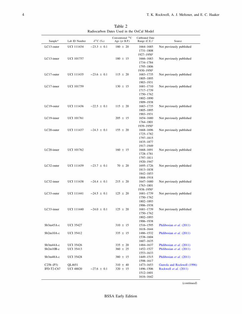
Table 2Radiocarbon Dates Used in the OxCal Model

Sample* Lab ID Number δ13C (‰)Conventional 14CAge (yr B.P.)

Calibrated DateRange (C.E.)† Source

LC13-outer UCI 111434 −23.3 ± 0.1 180 ± 20 1664–1685 Not previously published1731–18081927–1950‡

LC13-inner UCI 101757 180 ± 15 1666–1683 Not previously published1734–17841795–18061930–1950‡

LC17-outer UCI 111435 −23.6 ± 0.1 115 ± 20 1683–1735 Not previously published1805–18951903–1931

LC17-inner UCI 101759 130 ± 15 1681–1710 Not previously published1717–17391750–17621802–18901909–1938

LC19-outer UCI 111436 −22.5 ± 0.1 115 ± 20 1683–1735 Not previously published1805–18951903–1931

LC19-inner UCI 101761 205 ± 15 1654–1680 Not previously published1764–18011939–1950‡

LC20-outer UCI 111437 −24.3 ± 0.1 155 ± 20 1668–1696 Not previously published1725–17821797–18151835–18771917–1949

LC20-inner UCI 101762 160 ± 15 1668–1691 Not previously published1728–17811797–18111920–1947

LC32-outer UCI 111439 −23.7 ± 0.1 70 ± 20 1695–1726 Not previously published1813–18381842–18531868–1918

LC32-inner UCI 111438 −24.4 ± 0.1 215 ± 20 1647–1680 Not previously published1763–18011938–1950‡

LC33-outer UCI 111441 −24.5 ± 0.1 125 ± 20 1681–1739 Not previously published1750–17621802–18931906–1938

LC33-inner UCI 111440 −24.0 ± 0.1 125 ± 20 1681–1739 Not previously published1750–17621802–18931906–1938

Sb3m45A-c UCI 35427 310 ± 15 1516–1595 Philibosian et al. (2011)1618–1644

Sb2m10A-c UCI 35412 335 ± 15 1486–1532 Philibosian et al. (2011)1538–16041607–1635

Sb3m44A-c UCI 35426 335 ± 20 1484–1637 Philibosian et al. (2011)Sb2m10B-c UCI 35413 360 ± 25 1452–1527 Philibosian et al. (2011)

1553–1633Sb3m48A-c UCI 35428 380 ± 15 1449–1515 Philibosian et al. (2011)

1598–1617C25b (P3) QL4651 310 ± 40 1473–1653 Gurrola and Rockwell (1996)IFD-T2-C67 UCI 48820 −27.6 ± 0.1 320 ± 15 1496–1506 Rockwell et al. (2011)

1512–16011616–1642

(continued)

4 T. K. Rockwell, A. J. Meltzner, and E. C. Haaker

BSSA Early Edition

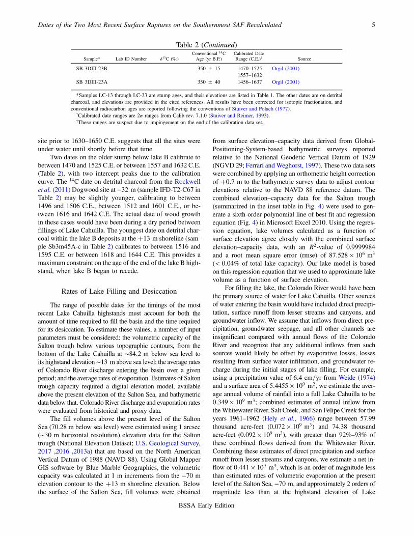
site prior to 1630–1650 C.E. suggests that all the sites wereunder water until shortly before that time.

Two dates on the older stump below lake B calibrate tobetween 1470 and 1525 C.E. or between 1557 and 1632 C.E.(Table 2), with two intercept peaks due to the calibrationcurve. The 14C date on detrital charcoal from the Rockwellet al. (2011) Dogwood site at −32 m (sample IFD-T2-C67 inTable 2) may be slightly younger, calibrating to between1496 and 1506 C.E., between 1512 and 1601 C.E., or be-tween 1616 and 1642 C.E. The actual date of wood growthin these cases would have been during a dry period betweenfillings of Lake Cahuilla. The youngest date on detrital char-coal within the lake B deposits at the�13 m shoreline (sam-ple Sb3m45A-c in Table 2) calibrates to between 1516 and1595 C.E. or between 1618 and 1644 C.E. This provides amaximum constraint on the age of the end of the lake B high-stand, when lake B began to recede.

Rates of Lake Filling and Desiccation

The range of possible dates for the timings of the mostrecent Lake Cahuilla highstands must account for both theamount of time required to fill the basin and the time requiredfor its desiccation. To estimate these values, a number of inputparameters must be considered: the volumetric capacity of theSalton trough below various topographic contours, from thebottom of the Lake Cahuilla at ∼84:2 m below sea level toits highstand elevation∼13 m above sea level; the average ratesof Colorado River discharge entering the basin over a givenperiod; and the average rates of evaporation. Estimates of Saltontrough capacity required a digital elevation model, availableabove the present elevation of the Salton Sea, and bathymetricdata below that. Colorado River discharge and evaporation rateswere evaluated from historical and proxy data.

The fill volumes above the present level of the SaltonSea (70.28 m below sea level) were estimated using 1 arcsec(∼30 m horizontal resolution) elevation data for the Saltontrough (National Elevation Dataset; U.S. Geological Survey,

2013,2016,2017 a) that are based on the North AmericanVertical Datum of 1988 (NAVD 88). Using Global MapperGIS software by Blue Marble Geographics, the volumetriccapacity was calculated at 1 m increments from the −70 melevation contour to the �13 m shoreline elevation. Belowthe surface of the Salton Sea, fill volumes were obtained

from surface elevation–capacity data derived from Global-Positioning-System-based bathymetric surveys reportedrelative to the National Geodetic Vertical Datum of 1929(NGVD 29; Ferrari andWeghorst, 1997). These two data setswere combined by applying an orthometric height correctionof �0:7 m to the bathymetric survey data to adjust contourelevations relative to the NAVD 88 reference datum. Thecombined elevation–capacity data for the Salton trough(summarized in the inset table in Fig. 4) were used to gen-erate a sixth-order polynomial line of best fit and regressionequation (Fig. 4) in Microsoft Excel 2010. Using the regres-sion equation, lake volumes calculated as a function ofsurface elevation agree closely with the combined surfaceelevation–capacity data, with an R2-value of 0.9999984and a root mean square error (rmse) of 87:528 × 106 m3

(< 0:04% of total lake capacity). Our lake model is basedon this regression equation that we used to approximate lakevolume as a function of surface elevation.

For filling the lake, the Colorado River would have beenthe primary source of water for Lake Cahuilla. Other sourcesof water entering the basin would have included direct precipi-tation, surface runoff from lesser streams and canyons, andgroundwater inflow. We assume that inflows from direct pre-cipitation, groundwater seepage, and all other channels areinsignificant compared with annual flows of the ColoradoRiver and recognize that any additional inflows from suchsources would likely be offset by evaporative losses, lossesresulting from surface water infiltration, and groundwater re-charge during the initial stages of lake filling. For example,using a precipitation value of 6:4 cm=yr from Weide (1974)and a surface area of 5:4455 × 109 m2, we estimate the aver-age annual volume of rainfall into a full Lake Cahuilla to be0:349 × 109 m3; combined estimates of annual inflow fromtheWhitewater River, Salt Creek, and San Felipe Creek for theyears 1961–1962 (Hely et al., 1966) range between 57.99thousand acre-feet (0:072 × 109 m3) and 74.38 thousandacre-feet (0:092 × 109 m3), with greater than 92%–93% ofthese combined flows derived from the Whitewater River.Combining these estimates of direct precipitation and surfacerunoff from lesser streams and canyons, we estimate a net in-flow of 0:441 × 109 m3, which is an order of magnitude lessthan estimated rates of volumetric evaporation at the presentlevel of the Salton Sea, −70 m, and approximately 2 orders ofmagnitude less than at the highstand elevation of Lake

Table 2 (Continued)

Sample* Lab ID Number δ13C (‰)Conventional 14CAge (yr B.P.)

Calibrated DateRange (C.E.)† Source

SB 3DIII-23B 350 ± 15 1470–1525 Orgil (2001)1557–1632

SB 3DIII-23A 350 ± 40 1456–1637 Orgil (2001)

*Samples LC-13 through LC-33 are stump ages, and their elevations are listed in Table 1. The other dates are on detritalcharcoal, and elevations are provided in the cited references. All results have been corrected for isotopic fractionation, andconventional radiocarbon ages are reported following the conventions of Stuiver and Polach (1977).

†Calibrated date ranges are 2σ ranges from Calib rev. 7.1.0 (Stuiver and Reimer, 1993).‡These ranges are suspect due to impingement on the end of the calibration data set.

Dates of the Two Most Recent Surface Ruptures on the Southernmost SAF Recalculated 5

BSSA Early Edition

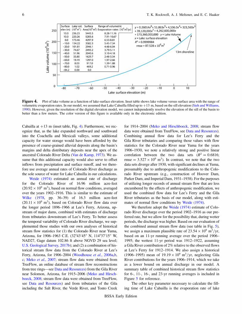
Cahuilla at �13 m (inset table, Fig. 4). Furthermore, we rec-ognize that, as the lake expanded northward and southwardinto the Coachella and Mexicali valleys, some additionalcapacity for water storage would have been afforded by thepresence of coarse-grained alluvial deposits along the basin’smargins and delta distributary deposits near the apex of theancestral Colorado River Delta (Van de Kamp, 1973). We as-sume that this additional capacity would also serve to offsetinflows from precipitation and surface runoff, and we there-fore use average annual rates of Colorado River discharge asthe sole source of water for Lake Cahuilla in our calculations.

Weide (1974) estimated an annual rate of dischargefor the Colorado River of 16.96 million acre-feet(20:92 × 109 m3), based on normal flow conditions, averagedover the years 1902–1916. This is similar to the estimate ofWilke (1978, pp. 36–39) of 16.3 million acre-feet(20:11 × 109 m3), based on Colorado River flow data overthe longer period 1896–1966 at Lee’s Ferry, Arizona, up-stream of major dams, combined with estimates of dischargefrom tributaries downstream of Lee’s Ferry. To better assessthe temporal variability of Colorado River discharge, we sup-plemented those studies with our own analyses of historicalstream flow statistics for (1) the Colorado River near Yuma,Arizona, for 1906–1963 C.E. (32°43′45″ N, 114°37′15″ W,NAD27, Gage datum 102.86 ft above NGVD 29 sea level;U.S. Geological Survey, 2017b); and (2) a combination of his-torical stream flow data from the Colorado River at Lee’sFerry, Arizona, for 1906–2004 (Woodhouse et al., 2006a,b,c; Meko et al., 2007; stream flow data were obtained fromTreeFlow, an online database of stream flow reconstructionsfrom tree rings—see Data and Resources) from the Gila Rivernear Solomon, Arizona, for 1915–2006 (Meko and Hirsch-boeck, 2008; stream flow data were obtained from TreeFlow,see Data and Resources) and from tributaries of the Gilaincluding the Salt River, the Verde River, and Tonto Creek

for 1914–2004 (Meko and Hirschboeck, 2008; stream flowdata were obtained from TreeFlow, see Data and Resources).Combining annual flow data for Lee’s Ferry and theGila River tributaries and comparing those values with flowstatistics for the Colorado River near Yuma for the years1906–1930, we note a relatively strong and positive linearcorrelation between the two data sets (R2 � 0:6816;rmse � 3:527 × 109 m3). In contrast, we note that the twodata sets diverge after 1930, with significant declines at Yuma,presumably due to anthropogenic modifications to the Colo-rado River upstream (e.g., construction of Hoover Dam,Parker Dam, and Imperial Dam, 1931–1938). For the purposesof utilizing longer records of annual stream flow that are lessencumbered by the effects of anthropogenic modification, weused the combined flow data for Lee’s Ferry and the GilaRiver tributaries as the basis of our model, along with esti-mates of normal flow conditions by Weide (1974).

We therefore adopt the Weide (1974) estimate of Colo-rado River discharge over the period 1902–1916 as our pre-ferred rate, but we allow for the possibility that, during wetterperiods, the discharge was higher. Based on our evaluation ofthe combined annual stream flow data (see table in Fig. 5),we assign a maximum plausible rate of 23:54 × 109 m3=yr,based on an 11-yr running average over the period 1906–1995; the wettest 11-yr period was 1912–1922, assuminga Gila River contribution of 2% relative to the observed flowsat Lee’s Ferry for 1912–1914. We also assign a historical(1906–1995) mean of 19:19 × 109 m3=yr, neglecting GilaRiver contributions for the years 1906–1914, which we takeas a lower bound on annual discharge in our model. Asummary table of combined historical stream flow statisticsfor 6-, 11-, 16-, and 23-yr running averages is included inFigure 5 for reference.

The other key parameter necessary to calculate the fill-ing time of Lake Cahuilla is the evaporation rate of lake

Figure 4. Plot of lake volume as a function of lake-surface elevation. Inset table shows lake volume versus surface area with the range ofvolumetric evaporation rates. In our model, we assumed that Lake Cahuilla filled up to�13 m, based on the sill elevation (Sieh andWilliams,1990). However, given the resolution of the digital elevation model, we cannot independently resolve the elevation of the sill of the basin tobetter than a few meters. The color version of this figure is available only in the electronic edition.

6 T. K. Rockwell, A. J. Meltzner, and E. C. Haaker

BSSA Early Edition

water. Evaporation rates for the desiccation of Lake Cahuillahave been variously estimated at 1:52–1:55 m=yr (Sieh andWilliams, 1990) to 1:8 m=yr (Wilke, 1978, p. 38). A fasterevaporation rate was directly measured from a water surfacein a tank in Calexico from 1904 to 1906 with an averageannual rate of 2:05 m=yr (Blake, 1915, p. 21), although overthose 3 yrs alone the evaporation ranged from 1.6 to2:6 m=yr. An even faster evaporation rate of ∼2:08 m=yris estimated for the Salton Sea on the U.S. Weather Bureau’sEvaporation Maps for the United States (Kohler et al., 1959,plate 2; Meyers and Nordenson, 1962, plate 3; Hely andPeck, 1964, plate 2). However, as Hely et al. (1966,pp. C18–C19) note, the evaporation rates shown on theEvaporation Maps for the United States should be approx-imately correct for evaporation from small bodies of freshwater; the larger effective diameter of the Salton Sea (andLake Cahuilla) would increase the humidity of the air mov-ing across the water surface, thereby decreasing the evapo-ration rate from that predicted by Kohler et al. (1959),Meyers and Nordenson (1962), and Hely and Peck (1964).In light of the aforementioned estimates, we adopt 1.52, 1.80,and 2:05 m=yr as plausible evaporation rates in our model.

Hydrologic Modeling and Time Requiredto Fill Lake Cahuilla

Using the input parameters described above, we devel-oped a hydrologic model for estimating the time required topartially fill Lake Cahuilla to the elevations of our dated

stump samples and to completely fill it to the �13 m shore-line. The sixth-order polynomial regression equation gener-ated from the 1 m elevation–capacity data for the Saltontrough Qnet � f�Heq� was used to convert lake volumes(Qnet) to equivalent lake-surface elevations (Heq). Completecapture of annual Colorado River discharge (Qin) was as-sumed constant for each year and added to the net volumeof lake water (Qnet) from the previous year; this yieldedthe initial volume of lake water (Qinitial) for each year, priorto evaporation. Starting with an empty basin (Qnet � 0,Heq � −84:2 m), water entering the basin each year (Qin)would result in an initial lake volume (Qinitial), causing thesurface elevation of the lake (Heq) to rise to an initial surfaceelevation (Hinitial); values of Qinitial were converted to valuesof Hinitial (Qinitial → Hinitial) by linear interpolation of theregression equation calculated at 0.1 m increments of equiv-alent surface elevation. After the value of Hinitial was deter-mined, evaporation would lower the surface of the lakelinearly by an amount equal to the average annual evapora-tion rate (ΔHevap), assumed to be constant for each year,resulting in the final surface elevation of the lake at theend of each model year. To repeat the calculation for the fol-lowing year, values ofHeq were converted back to equivalentlake volumes using the regression equation Qnet � f�Heq�.This process was repeated for subsequent years until Heq forthe final year equaled or exceeded the 13 m shoreline eleva-tion. To approximate the amount of time (t) required to fillthe lake completely (Heq � �13 m) and partially fill it to theelevations of our stump samples (Heq � stump elevation),

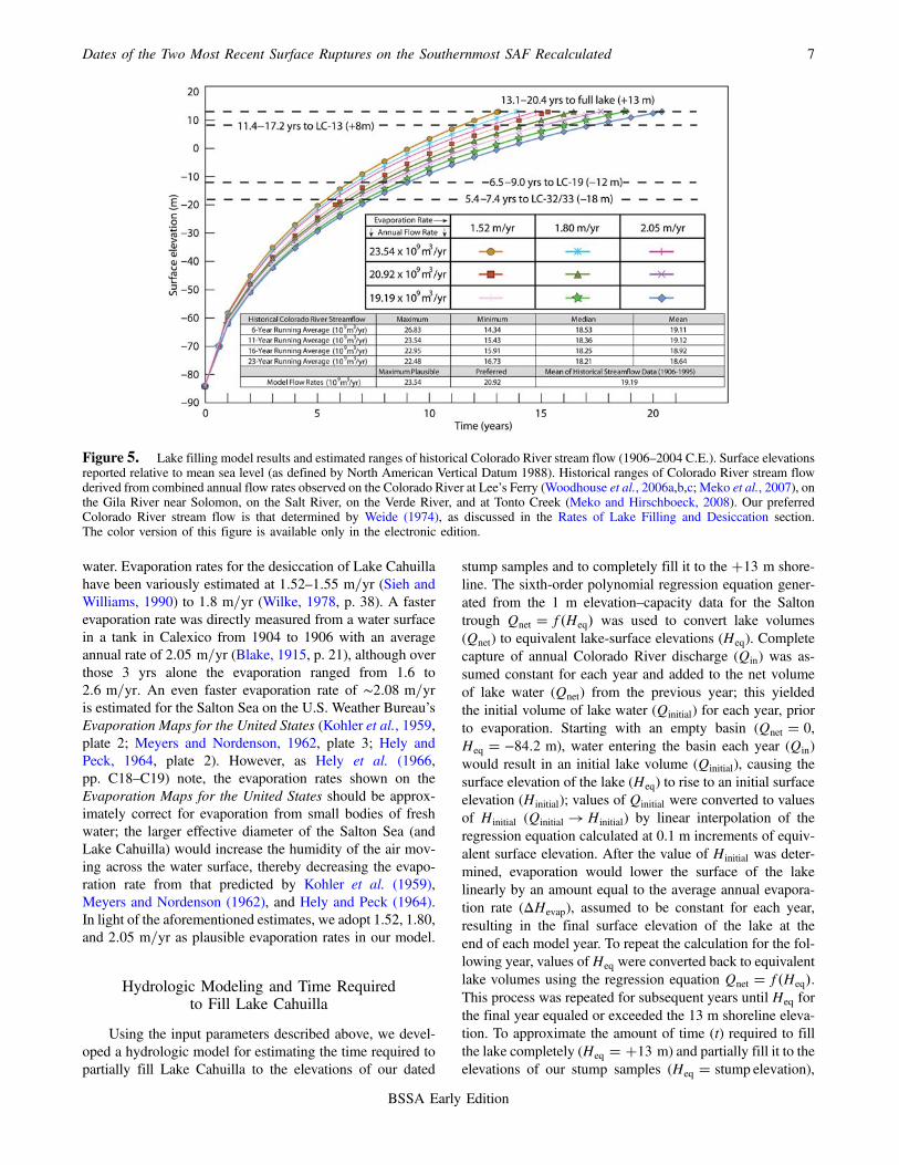
Figure 5. Lake filling model results and estimated ranges of historical Colorado River stream flow (1906–2004 C.E.). Surface elevationsreported relative to mean sea level (as defined by North American Vertical Datum 1988). Historical ranges of Colorado River stream flowderived from combined annual flow rates observed on the Colorado River at Lee’s Ferry (Woodhouse et al., 2006a,b,c; Meko et al., 2007), onthe Gila River near Solomon, on the Salt River, on the Verde River, and at Tonto Creek (Meko and Hirschboeck, 2008). Our preferredColorado River stream flow is that determined by Weide (1974), as discussed in the Rates of Lake Filling and Desiccation section.The color version of this figure is available only in the electronic edition.

Dates of the Two Most Recent Surface Ruptures on the Southernmost SAF Recalculated 7

BSSA Early Edition

we used linear interpolation to approximate the value of t as afunction of Heq between model years bracketing the desiredvalue of Heq. A total of nine simulations were run usingannual Colorado River discharge rates of 23:54 × 109,20:92 × 109, and 19:19 × 109 m3 in combination with an-nual evaporation rates of 1.52, 1.80, and 2:05 m=yr. The re-sults of our hydrologic modeling are summarized in Figure 5.

The results of the model suggest it would have takenbetween 13.1 and 20.4 yrs to completely fill Lake Cahuilla,and using our “preferred” discharge rate (20:92 × 109 m3),we provide a best estimate of 15.3–17.7 yrs. It would takeonly 5.4–7.4 yrs to fill the basin to the elevation of our lowestdated stump (LC-32/33) at approximately −18 m. If the pre-vious lake had not fully desiccated, less time would havebeen required.

Historical Constraints

Several early Spanish explorers made expeditions to themouth of the Colorado River, starting with Francisco deUlloa in 1539 (Bancroft, 1884, pp. 78–81; Wagner, 1929,pp. 19–20 and 307) and Hernando de Alarcón in 1540 (Ban-croft, 1884, pp. 90–93; Hammond and Rey, 1940, pp. 124–155). This continued 65 yrs later with Don Juan de Oñate andFather Francisco de Escobar in 1605 (Bolton, 1916, pp. 268–280; Bolton, 1919a) and then 95 yrs after that with a seriesof expeditions by Father Eusebio Francisco Kino between1700 and 1706 (Venegas, 1759, Vol. 1, pp. 300–311; Bolton,1919b, Vol. 1, pp. 246–256, 312–320, 340–345, and Vol. 2,pp. 205–214). Finally, Father Juan de Ugarte reached themouth of the Colorado River in 1721 (Venegas, 1759, Vol.2, pp. 46–62), as did Father Ferdinand Konščak (FernandoConsag) in 1746 (Venegas, 1759, Vol. 2, pp. 308–353). Detailsare in Appendix A, and locations mentioned here in the His-torical Constraints section are shown in Figure A1. None ofthese explorers reached the Salton trough, but in 1540, 1605,and 1700–1706, their accounts indicate that the ColoradoRiver was flowing to the Gulf of California at those times.

Another European explorer, Jacobo Sedelmayer (JocoboSedelmair), made a number of overland expeditions to theGila and Colorado Rivers between 1744 and 1750 (Venegas,1759, Vol. 2, pp. 181–211; Bancroft, 1884, pp. 536–543;Dunne, 1955). It appears that the only time during whichSedelmair followed the Colorado for any significant distancedownstream of its confluence with the Gila River was in1750, when he reached a point west of the sand dunes ofthe Gran Desierto de Altar that he subsequently crossed(Dunne, 1955, pp. 69–72). Sedelmair’s journey along theColorado River almost to the Gulf of California suggeststhe river was, once again, flowing southward to the Gulf.However, an unusual story related to Sedelmair in 1748suggests that the Colorado River flowed, at least partiallyor intermittently, into the Salton trough. Sedelmair recountsa story told to him by Yuma Indians, while he was stationedjust east of the confluence of the Colorado and Gila Rivers:“Here they informed me that if one crossed the Colorado and

traveled northwest for two days one would touch once againthe banks of the same river” (Dunne, 1955, p. 60). Later,Bancroft (1884, pp. 541–543) discusses a letter written in1751 to the king of Spain, in which Captain FernandoSanchez Salvador “advances the theory that the Colorado be-fore reaching the gulf throws off a branch to the westward,which flows into the Pacific between Monterey and PointConcepcion.” Although the details of a river reaching thePacific are clearly impossible, the theory was likely based onthe reports of the natives, and it suggests that, at least in whatwas then recent memory, the Colorado River had flowed, inpart, into the Salton trough. And although Kino had visitedwith the same tribes at the same location in 1700, 1701, andagain in 1702, no stories emerged during any of Kino’s visitsof a westward distributary of the Colorado River.

A series of expeditions between 1771 and 1776unequivocally demonstrate the absence of a lake in theSalton trough at that time. In 1771, although Father Fran-cisco Garcés was confused about his location at the time, hefollowed the Colorado River from its confluence with theGila southward to the head of tidewater, near Heintzelman’sPoint (Bolton, 1917, pp. 322–325). From there, Garcés trav-eled northwestward, reaching a point about three leagues eastof present-day Yuha Well; at that point, he was forced to turnaround because he was out of water and had lost hope offinding water farther along (Bolton, 1917, pp. 325–328; Bol-ton, 1930, Vol. 1, pp. 45–47 and opposite p. 120, and Vol. 2,pp. 337–338).

Starting in 1774, Juan Bautista de Anza, Father Fran-cisco Garcés, Father Pedro Font, and Juan Díaz continuedto explore the region, searching for a land route to the westcoast. On 10–11 March and 7–8 May 1774 (Bolton, 1930,Vol. 2, pp. 81–85, 113–114, 194–197, 228, 280–281, 296,338–341) and again on 13–18 December 1775 and 7–8May 1776 (Bolton, 1930, Vol. 3, pp. 56–62, 172–174, 195,229–230, 295–296, and Vol. 4, pp. 129–140, 478–481),Anza and his party camped at a site they named San Sebas-tián, on San Felipe Creek near its confluence with CarrizoWash, at an elevation of −40 to −35 m, near 33.099° N,115.925° W. On 8 May 1774, both Anza and Díaz wrote intheir diaries about looking for watering holes to the east orsoutheast of San Sebastián (Bolton, 1930, Vol. 2, pp. 114,228, 296); exactly 2 yrs later, on 8 May 1776, Anza and Fontdescribed searching once again for a watering hole in thatvicinity (Bolton, 1930, Vol. 3, pp. 173–174, 296, and Vol.4, pp. 479–481), and this time they made it to Kane Spring,at 33.110° N, 115.836° W and −43 m. Despite their efforts,Font stated definitively on 8 May 1776 that the water at KaneSpring was “all the water we found” until they reached somewells at Pozo Salobre del Carrizal, where Font found “thewater as red as if it had vermilion [and] very salty” (Bolton,1930, Vol. 4, p. 481; see also, Vol. 3, p. 174). Bolton placesthe Pozo Salobre del Carrizal site on the old Paredones River,south of Cocopah in Baja California; Cocopah (EstaciónCucapah) is present-day Ejido Tamaulipas, at 32.550° N,115.232° W, and in the early twentieth century the Paredones

8 T. K. Rockwell, A. J. Meltzner, and E. C. Haaker

BSSA Early Edition

River was 5–10 km south of that point (Bolton, 1930, Vol. 1,opposite p. 120; see also Cory, 1915, p. 1219). No mention isever made in any of the diaries of finding a body of water ofany size in the center of the Salton trough, indicating that themost recent lake (lake A) must have desiccated completely ornearly completely by 1774. Furthermore, in his diary on 10March 1774, Díaz described the diet of the natives who livednear the San Sebastián site, and it included mesquite beans(Bolton, 1930, Vol. 2, p. 280); if mature mesquite trees weregrowing at −35 m in 1774, the lake must have desiccated tobelow that elevation many years before then.

We use the historical accounts to place constraints onwhen the Colorado River was flowing to the Gulf, in whichcase we interpret that the lake was not in a filling phase. Wealso use Anza’s traverse of the region as a hard constraint asto when the lake was mostly or completely dry, which limitshow recently a complete filling could have occurred.

Climate Proxy Data

The stump ages (Table 2) require that the most recentLake Cahuilla (lake A) must have filled around or after thebeginning of the eighteenth century, and if we account for thetime required to desiccate the lake from �13 m to −84:2 m,then historical accounts limit the filling of the most recentLake Cahuilla to the early eighteenth century or earlier. Weare therefore particularly interested in rainfall on the Colo-rado River catchment area in the early eighteenth century.Climate proxy records from the lower and upper ColoradoRiver basin reveal decadal variations in rainfall. Precipitationon the lower Colorado River basin averaged 30:0 cm=yr over1902–1916; the period 1707–1717 was drier, with precipita-tion averaging 26:3 cm=yr, whereas 1718–1727 was wetter,with precipitation averaging 33:8 cm=yr (Salzer and Kipf-mueller, 2005a,b). For the upper Colorado River, annualflows at Lee’s Ferry were reconstructed from tree rings(Woodhouse et al., 2006a,b,c; Meko et al., 2007; stream flowdata were obtained from TreeFlow,see Data and Resources).The period 1902–1916 saw an average annual flow at Lee’sFerry of 19:4 × 109 m3=yr, whereas 1707–1717 was drier,with an average flow of 17:5 × 109 m3=yr, and 1718–1727was wetter, with an average flow of 20:9 × 109 m3=yr. Thesepaleoclimate reconstructions consistently show that theColorado River catchment area was ∼10% drier in 1707–1717, and ∼10% wetter in 1718–1727, relative to the1902–1916 baseline. This implies that, depending on the ex-act timing of the most recent filling of Lake Cahuilla, it mayhave been possible to trim a year or so off the time required tofill the lake, but at other times it might have required an extrayear. In any case, if the most recent lake did not begin fillinguntil after Kino’s final visit in 1706, the full lake highstand isnot likely to have occurred until after 1721 C.E. or perhaps ayear or two earlier if there was already some water in thebasin in 1706; if the most recent lake did not begin fillinguntil 1718 C.E., the full lake highstand is not likely to haveoccurred until after 1731 C.E. or perhaps a year or two earlier

if there was already some water in the basin. Although itseems reasonable to infer that an avulsion of the ColoradoRiver would be more likely during the wet period from1718 to 1727 than during the dry period from 1707 to 1717,we do not impose this as a prior constraint in our model.

As stated previously, desiccation rates for evaporation ofLake Cahuilla are estimated at 1:52–2:05 m=yr (Blake,1915, p. 21; Wilke, 1978, p. 38; Sieh and Williams, 1990),implying that between 47 and 64 yrs is required for full des-iccation from �13 to −84:2 m. If the Cahuilla basin hadcompletely desiccated by 1774, then the lake would havehad to start drying up between 1710 and 1727. However,if some saline water was still resident in the basin in1774, then the date of avulsion of the Colorado River backinto the Gulf of California (and the onset of desiccation)could be advanced by several years. Alternatively, if thefaster, historically documented evaporation rate from LakeMead is applied (2:18 m=yr; Hely et al., 1966, p. C18), thena slightly later date of 1731 is allowable for the end of lake Aat�13 m. In any case, the historical constraints provided byKino’s and Anza’s visits, along with the limits on the fillingand desiccation rates, provide strong bounds on the timing offilling and desiccation of lake A and therefore on the timingof the most recent large SAF earthquake.

Chronological Modeling and Final Ages

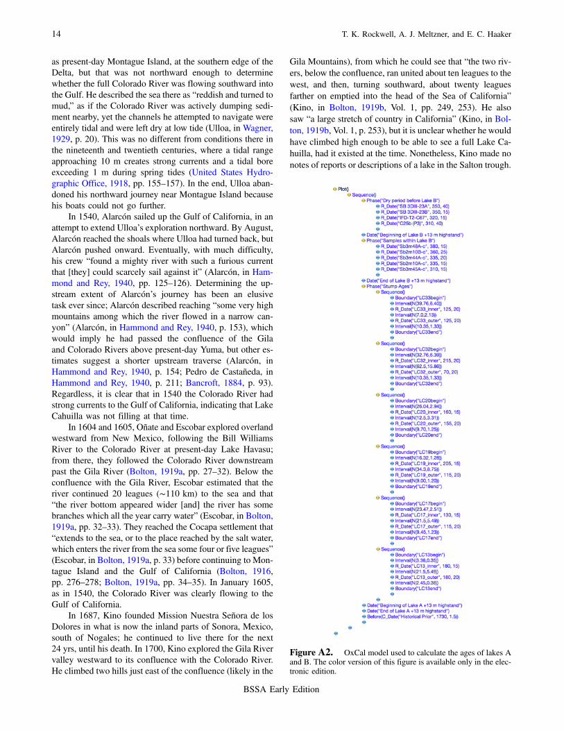
We constructed an OxCal model (Bronk Ramsey, 2008;Fig. 6 and Fig. A2) that incorporates four sets of constraints.Working backward in time, we impose a historical prior of1730� 3 C.E. (2σ) that represents the last date at whichLake Cahuilla could have been full (at �13 m elevation)if it had mostly or completely desiccated by the time ofAnza’s visit in 1774. The second set of constraints comesfrom the dated mesquite (Prosopis sp.) stumps that weregrowing in the footprint of Lake Cahuilla but which, we in-fer, were drowned by the last filling of the lake; these date thedry period between lakes A and B. The third set of con-straints consists of five samples from the lake B shorelinedeposits that provide a maximum limit on the age of the endof the lake B highstand. The oldest set consists of four addi-tional radiocarbon dates that date the dry period prior to lakeB (Fig. 6).

For each of the stumps that were killed by the filling oflake A, we ran radiocarbon dates on both the outermost andthe innermost preserved growth rings (Fig. 3), and wevisually counted the number of rings separating the outer-most and innermost preserved rings (Table 1). Because thecentral core of some of the stumps was missing, presumablyeaten by termites, we also crudely estimated (with appropri-ately large uncertainties) the number of years of growth thatwere missing from the center of the stump, based on thegrowth rate of mesquite (Ansley et al., 2010; Table 1). Toovercome the complication that the various stumps grew atdifferent elevations and therefore could have begun growingat different times, we estimated the number of years that it

Dates of the Two Most Recent Surface Ruptures on the Southernmost SAF Recalculated 9

BSSA Early Edition

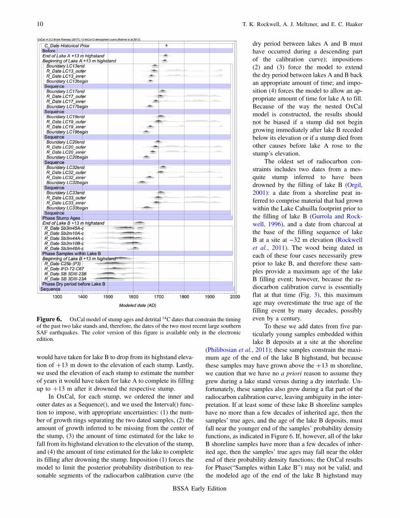
would have taken for lake B to drop from its highstand eleva-tion of �13 m down to the elevation of each stump. Lastly,we used the elevation of each stump to estimate the numberof years it would have taken for lake A to complete its fillingup to �13 m after it drowned the respective stump.

In OxCal, for each stump, we ordered the inner andouter dates as a Sequence(), and we used the Interval() func-tion to impose, with appropriate uncertainties: (1) the num-ber of growth rings separating the two dated samples, (2) theamount of growth inferred to be missing from the center ofthe stump, (3) the amount of time estimated for the lake tofall from its highstand elevation to the elevation of the stump,and (4) the amount of time estimated for the lake to completeits filling after drowning the stump. Imposition (1) forces themodel to limit the posterior probability distribution to rea-sonable segments of the radiocarbon calibration curve (the

dry period between lakes A and B musthave occurred during a descending partof the calibration curve); impositions(2) and (3) force the model to extendthe dry period between lakes A and B backan appropriate amount of time; and impo-sition (4) forces the model to allow an ap-propriate amount of time for lake A to fill.Because of the way the nested OxCalmodel is constructed, the results shouldnot be biased if a stump did not begingrowing immediately after lake B recededbelow its elevation or if a stump died fromother causes before lake A rose to thestump’s elevation.

The oldest set of radiocarbon con-straints includes two dates from a mes-quite stump inferred to have beendrowned by the filling of lake B (Orgil,2001): a date from a shoreline peat in-ferred to comprise material that had grownwithin the Lake Cahuilla footprint prior tothe filling of lake B (Gurrola and Rock-well, 1996), and a date from charcoal atthe base of the filling sequence of lakeB at a site at −32 m elevation (Rockwellet al., 2011). The wood being dated ineach of these four cases necessarily grewprior to lake B, and therefore these sam-ples provide a maximum age of the lakeB filling event; however, because the ra-diocarbon calibration curve is essentiallyflat at that time (Fig. 3), this maximumage may overestimate the true age of thefilling event by many decades, possiblyeven by a century.

To these we add dates from five par-ticularly young samples embedded withinlake B deposits at a site at the shoreline

(Philibosian et al., 2011); these samples constrain the maxi-mum age of the end of the lake B highstand, but becausethese samples may have grown above the �13 m shoreline,we caution that we have no a priori reason to assume theygrew during a lake stand versus during a dry interlude. Un-fortunately, these samples also grew during a flat part of theradiocarbon calibration curve, leaving ambiguity in the inter-pretation. If at least some of these lake B shoreline sampleshave no more than a few decades of inherited age, then thesamples’ true ages, and the age of the lake B deposits, mustfall near the younger end of the samples’ probability densityfunctions, as indicated in Figure 6. If, however, all of the lakeB shoreline samples have more than a few decades of inher-ited age, then the samples’ true ages may fall near the olderend of their probability density functions; the OxCal resultsfor Phase(“Samples within Lake B”) may not be valid, andthe modeled age of the end of the lake B highstand may

Figure 6. OxCal model of stump ages and detrital 14C dates that constrain the timingof the past two lake stands and, therefore, the dates of the two most recent large southernSAF earthquakes. The color version of this figure is available only in the electronicedition.

10 T. K. Rockwell, A. J. Meltzner, and E. C. Haaker

BSSA Early Edition

underestimate the true age by many decades, possibly evenby a century. In spite of the aforementioned complications,we can robustly conclude that the lake B highstand began noearlier than 1550� 40 C.E. (2σ) and ended no later than1624� 20 C.E. (2σ). The actual timing of lake B couldbe anywhere in that interval, and the duration of the lakeB highstand is not tightly constrained by these data (Fig. 7).

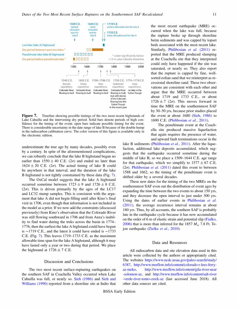
The OxCal model suggests that the lake A highstandoccurred sometime between 1723� 9 and 1726� 8 C.E.(2σ). This is driven primarily by the ages of the LC17and LC32 stump samples. This is consistent with the argu-ment that lake A did not begin filling until after Kino’s finalvisit in 1706, even though that information is not included inthe model as a prior. If we now add the constraints (discussedpreviously) from Kino’s observation that the Colorado Riverwas still flowing southward in 1706 and from Anza’s inabil-ity to find water during the treks across the basin in 1774–1776, then the earliest the lake A highstand could have begunis ∼1719 C.E., and the latest it could have ended is ∼1733C.E. (Fig. 7). This leaves 1719–1733 C.E. as the maximumallowable time span for the lake A highstand, although it mayhave lasted only a year or two during that period. We placethe highstand at 1726� 7 C.E.

Discussion and Conclusions

The two most recent surface-rupturing earthquakes onthe southern SAF in Coachella Valley occurred when LakeCahuilla was full, or nearly so. Sieh (1986) and Sieh andWilliams (1990) reported from a shoreline site at Indio that

the most recent earthquake (MRE) oc-curred when the lake was full, becausethe rupture broke up through shorelineberm sediments and was capped by topsetbeds associated with the most recent lake.Similarly, Philibosian et al. (2011) re-ported that the MRE produced slumpingat the Coachella site that they interpretedcould only have happened if the site wassaturated, or nearly so. They also reportthat the rupture is capped by fine, well-sorted eolian sand that we reinterpret as re-cessional shoreline sand. These two obser-vations are consistent with each other andargue that the MRE occurred betweenabout 1719 and 1733 C.E., or about1726� 7 (2σ). This moves forward intime the MRE on the southernmost SAFby 30–50 yrs, because prior studies placedthe event at about 1680 (Sieh, 1986) to1690 C.E. (Philibosian et al., 2011).

The penultimate event at the Coach-ella site produced massive liquefactionthat again requires the presence of water,and upward fault terminations occur in the

lake B sediments (Philibosian et al., 2011). After the lique-faction, additional lake deposits accumulated, which sug-gests that the earthquake occurred sometime during themiddle of lake B, so we place a 1509–1644 C.E. age rangefor that earthquake, which we simplify to 1577� 67 C.E.(2σ). Philibosian et al. (2011) dated this event to between1588 and 1662, so the timing of the penultimate event isshifted older by a several decades.

These new dates for the timing of the two MREs on thesouthernmost SAF even out the distribution of event ages byexpanding the time between the two events to about 150 yrs,and they decrease the open interval to just under 300 yrs.Using the dates of earlier events in Philibosian et al.(2011), the average recurrence interval remains at about180 yrs. Thus, by all accounts, the southern SAF is probablylate in the earthquake cycle because it has now accumulatedon the order of 6 m of elastic strain and potential slip (Fialko,2006) that is more than inferred for the 1857 Mw 7.8 Ft. Te-jon earthquake (Zielke et al., 2010).

Data and Resources

All radiocarbon data and site elevation data used in thisarticle were collected by the authors or appropriately cited.The websites https://www.ncdc.noaa.gov/paleo‑search/study/6387, http://www.treeflow.info/content/colorado-r-lees-ferry-az-meko, http://www.treeflow.info/content/gila-river-near-solomon-az, and http://www.treeflow.info/content/salt-river-verde-river-tonto-creek-az (last accessed June 2018). Allother data sources are cited.

Figure 7. Timeline showing possible timings of the two most recent highstands ofLake Cahuilla and the intervening dry period. Solid bars denote periods of high con-fidence for the timing of the event; open bars indicate possible timing for the event.There is considerable uncertainty in the date range of lake B because of the double humpin the radiocarbon calibration curve. The color version of this figure is available only inthe electronic edition.

Dates of the Two Most Recent Surface Ruptures on the Southernmost SAF Recalculated 11

BSSA Early Edition

Acknowledgments

The authors thank the reviewers (Neta Wechsler and anonymous) forimproving the presentation of this article. This work was supported by theSouthern California Earthquake Center (SCEC) Grant Numbers 12170 and14049. This research was also supported by the National Research Founda-tion Singapore and the Singapore Ministry of Education under the ResearchCentres of Excellence initiative. This is SCEC Contribution Number 7970and Earth Observatory of Singapore Contribution Number 179.

References

Ansley, R. J., M. Mirik, and M. J. Castellano (2010). Structural biomasspartitioning in regrowth and undisturbed mesquite (Prosopis glandu-losa): Implications for bioenergy uses, GCB Bioenergy 2, 26–36, doi:10.1111/j.1757-1707.2010.01036.x.

Bancroft, H. H. (1884). History of the North Mexican States, Vol. 1,A.L. Bancroft & Company, San Francisco, California, 1531–1800.

Blake, W. P. (1915). Sketch of the region at the head of the Gulf ofCalifornia, in The Imperial Valley and the Salton Sink, H. T. Cory(Editor), John J. Newbegin, San Francisco, California, 1–35.

Bolton, H. E. (1916). Spanish Exploration in the Southwest, CharlesScribner’s Sons, New York, New York, 1542–1706.

Bolton, H. E. (1917). The early explorations of Father Garcés on the Pacificslope, in The Pacific Ocean in History, H. M. Stephens and H. E. Bol-ton (Editors), Macmillan Company, New York, New York, 317–330.

Bolton, H. E. (1919a). Father Escobar’s relation of the Oñate expedition toCalifornia, Catholic Hist. Rev. 5, 19–41.

Bolton, H. E. (1919b). Kino’s Historical Memoir of Pimería Alta, 2 Vols.,Arthur H. Clark Company, Cleveland, Ohio.

Bolton, H. E. (1930). Anza’s California Expeditions, 5 Vols., University ofCalifornia Press, Berkeley, California.

Bronk Ramsey, C. (2008). Deposition models for chronological records,Quaternary Sci. Rev. 27, 42–60, doi: 10.1016/j.quascirev.2007.01.019.

Cory, H. T. (1915). The Imperial Valley and the Salton Sink, John J. New-begin, San Francisco, California.

Dunne, P. M. (1955). Jacobo Sedelmayr: Missionary, Frontiersman, Ex-plorer in Arizona and Sonora, Arizona Pioneers’ Historical Society,Tucson, Arizona.

Ferrari, R. L., and P. Weghorst (1997). Salton Sea 1995 Hydrographic GPSSurvey, U.S. Department of the Interior, Bureau of Reclamation, 24 pp.

Fialko, Y. (2006). Interseismic strain accumulation and the earthquakepotential on the southern San Andreas fault system, Nature 441,968–971.

Field, E. H., G. P. Biasi, P. Bird, T. E. Dawson, K. R. Felzer, D. D. Jackson,K. M. Johnson, T. H. Jordan, C. Madden, A. J. Michael, et al. (2015).Long-term time-dependent probabilities for the third Uniform Califor-nia Earthquake Rupture Forecast (UCERF3), Bull. Seismol. Soc. Am.105, 511–543, doi: 10.1785/0120140093.

Fumal, T. E., M. J. Rymer, and G. G. Seitz (2002). Timing of large earth-quakes since A.D. 800 on the Mission Creek strand of the San Andreasfault zone at Thousand Palms Oasis, near Palm Springs, California,Bull. Seismol. Soc. Am. 92, 2841–2860, doi: 10.1785/0120000609.

Gomberg, J., M. E. Belardinelli, M. Cocco, and P. Reasenberg (2005). Time-dependent earthquake probabilities, J. Geophys. Res. 110, no. B05S04,doi: 10.1029/2004JB003405.

Gurrola, L. D., and T. K. Rockwell (1996). Timing and slip for prehistoricearthquakes on the Superstition Mountain fault, Imperial Valley,southern California, J. Geophys. Res. 101, 5977–5985, doi:10.1029/95JB03061.

Haaker, E. C. (2012). Moving towards a more complete Late Holocenechronology of ancient Lake Cahuilla, B.S. Thesis, San Diego StateUniversity, San Diego, California, 19 pp.

Hammond, G. P., and A. Rey (1940). Narratives of the Coronado Expedi-tion, 1540–1542, University of New Mexico Press, Albuquerque,New Mexico, 413 pp.

Hely, A. G., and E. L. Peck (1964). Precipitation, runoff, and water loss inthe Lower Colorado River–Salton Sea area, U.S. Geol. Surv. Profess.Pap. 486-B, available at https://pubs.usgs.gov/pp/0486b/ (last accessedJune 2018).

Hely, A. G., G. H. Hughes, and B. Irelan (1966). Hydrologic regimen ofSalton Sea, California, U.S. Geol. Surv. Profess. Pap. 486-C, availableat https://pubs.usgs.gov/pp/0486c/ (last accessed June 2018).

Kohler, M. A., T. J. Nordenson, and D. R. Baker (1959). Evaporation mapsfor the United States, U.S. Weather Bur. Tech. Pap. 37.

Meko, D. M., and K. K. Hirschboeck (2008). The current drought in context:A tree-ring based evaluation of water supply variability for the Salt–Verde River basin, Final Report, available at http://www.treeflow.info/sites/default/files/SRP‑II‑Final‑Final‑Report‑08‑08‑08.pdf (last ac-cessed June 2018).

Meko, D. M., C. A. Woodhouse, C. A. Baisan, T. Knight, J. J. Lukas, M. K.Hughes, andM.W. Salzer (2007). Medieval drought in the upper Colo-rado River basin, Geophys. Res. Lett. 34, L10705, doi: 10.1029/2007GL029988.

Meyers, J. S., and T. J. Nordenson (1962). Evaporation from the 17 WesternStates, U.S. Geol. Surv. Profess. Pap. 272-D, available at https://pubs.usgs.gov/pp/0272d/ (last accessed June 2018).

Orgil, A. (2001). Three-dimensional paleoseismic investigation on the southbreak of the Coyote Creek fault, southern California, M.S. Thesis, SanDiego State University, San Diego, California, 85 pp.

Petersen, M. D., T. Cao, K. W. Campbell, and A. D. Frankel (2007).Time-independent and time-dependent seismic hazard assessmentfor the State of California: Uniform California Earthquake RuptureForecast Model 1.0. Seismol. Res. Lett. 78, 99–109, doi: 10.1785/gssrl.78.1.99.

Philibosian, B., T. Fumal, and R. Weldon (2011). San Andreas fault earth-quake chronology and Lake Cahuilla history at Coachella, California,Bull. Seismol. Soc. Am. 101, 13–38, doi: 10.1785/0120100050.

Reimer, P. J., E. Bard, A. Bayliss, J. W. Beck, P. G. Blackwell, C. BronkRamsey, C. E. Buck, H. Cheng, R. L. Edwards, M. Friedrich, et al.(2013). IntCal13 and Marine13 radiocarbon age calibration curves0-50,000 years cal BP, Radiocarbon 55, 1869–1887, doi: 10.2458/azu_js_rc.55.16947.

Rockwell, T. K., A. Meltzner, and R. Tsang (2011). A long record of earth-quakes with timing and displacements for the Imperial fault: A test ofearthquake recurrence models, Final Technical Report, U.S. Geologi-cal Survey, 28 pp.

Salzer, M. W., and K. F. Kipfmueller (2005a). Reconstructed temperatureand precipitation on a millennial timescale from tree-rings in thesouthern Colorado Plateau, U.S.A, Clim. Change 70, 465–487, doi:10.1007/s10584-005-5922-3 (last accessed June 2018).

Salzer, M. W., and K. F. Kipfmueller (2005b). Southern Colorado PlateauTemperature and Precipitation Reconstructions, IGBP PAGES/WorldData Center for Paleoclimatology, Data Contribution Series Number2005-066, NOAA/NCDC Paleoclimatology Program, Boulder,Colorado, available at ftp://ftp.ncdc.noaa.gov/pub/data/paleo/treering/reconstructions/northamerica/usa/colorado‑plateau2005.txt.

Sedelmair, J. (1750). Entrada a la nacion de los yumas gentiles por el mes deOctubre y Noviembre del año de 1749, in Documentos para la Historiade México, F. García Figueroa (Editor) (1856), quarta série (4th series),tomo I, Vol. 1, Vicente García Torres, Mexico City, 18–25 (in Spanish).

Sieh, K. E. (1986). Slip rate across the San Andreas and prehistoric earth-quakes at Indio, California, Eos Trans. AGU 67, 1200.

Sieh, K. E., and P. L. Williams (1990). Behavior of the southernmostSan Andreas fault during the past 300 years, J. Geophys. Res. 95,6629–6645, doi: 10.1029/JB095iB05p06629.

Stuiver, M., and H. A. Polach (1977). Discussion: Reporting of 14C data,Radiocarbon 19, 355–363, doi: 10.1017/S0033822200003672.

Stuiver, M., and P. J. Reimer (1993). Extended 14C data base and revisedCALIB 3.0 14C age calibration program, Radiocarbon 35, 215–230, doi: 10.1017/S0033822200013904.

United States Hydrographic Office (1918). Mexico and Central AmericanPilot (Pacific Coast) from the United States to Colombia including

12 T. K. Rockwell, A. J. Meltzner, and E. C. Haaker

BSSA Early Edition

the Gulfs of California and Panama, Fifth Ed., Government PrintingOffice, Washington, D.C.

U.S. Geological Survey (2013). USGS NED 1 arc-second n34w116 1 x 1degree ArcGrid, available at https://www.sciencebase.gov/catalog/item/581d26e1e4b08da350d5cd86 (last accessed June 2018).

U.S. Geological Survey (2016). USGS NED 1 arc-second n34w117 1 x 1degree ArcGrid (last accessed June 2018).

U.S. Geological Survey (2017a). USGS NED 1 arc-second n33w116 1 x 1degree ArcGrid, available at https://www.sciencebase.gov/catalog/item/581d25eee4b08da350d5b3ea (last accessed June 2018).

U.S. Geological Survey (2017b). USGS surface-water annual statistics forthe nation: USGS 09521000 Colorado River at Yuma, AZ, availableat https://waterdata.usgs.gov/nwis/annual?search_site_no=09521000&format=sites_selection_links (last accessed June 2018).

Van de Kamp, P. C. (1973). Holocene continental sedimentation in the SaltonBasin, California: A reconnaissance, Geol. Soc. Am. Bull. 84, 827–848,doi: 10.1130/0016-7606(1973)84<827:HCSITS>2.0.CO;2.

Venegas, M. (1757). Noticia de la California, y de su Conquista Temporal, yEspiritual hasta el Tiempo Presente, 3 Vols., La Imprenta de la Viudade Manuel Fernández, y del Supremo Consejo de la Inquisicion,Madrid (in Spanish).

Venegas, M. (1759). A Natural and Civil History of California, 2 Vols.,James Rivington and James Fletcher, London, United Kingdom.

Wagner, H. R. (1929). Spanish Voyages to the Northwest Coast of Americain the Sixteenth Century, California Historical Society, San Francisco,California, 571 pp.

Waters, M. R. (1983). Late Holocene lacustrine chronology and archaeologyof ancient Lake Cahuilla, California, Quaternary Res. 19, 373–387,doi: 10.1016/0033-5894(83)90042-X.

Weide, D. L. (1974). Regional environmental history of the Yuha Desertregion, in Background to Prehistory of the Yuha Desert Region, M.L. Weide, J. P. Barker, H. W. Lawton, D. L. Weide, and P. J. Wilke(Editors), Report for U.S. Department of Interior, Bureau of LandManagement, California Desert Planning Program, 4–15, doi:10.6067/XCV8X34WNH.

Wilke, P. J. (1978). Late prehistoric human ecology at Lake Cahuilla, Coach-ella Valley, California, Contributions of the University of CaliforniaArchaeological Research Facility, Department of Anthropology, Uni-versity of California Berkeley, No. 38, 168 pp., available at https://escholarship.org/uc/item/8367m039 (last accessed June 2018).

Woodhouse, C. A., S. T. Gray, and D. M. Meko (2006a). Updated stream-flow reconstructions for the Upper Colorado River basin, WaterResour. Res. 42, no. W05415, doi: 10.1029/2005WR004455.

Woodhouse, C. A., S.T. Gray, and D. M. Meko (2006b). Updated Stream-flow Reconstructions for the Upper Colorado River Basin, IGBPPAGES/World Data Center for Paleoclimatology, Data ContributionSeries Number 2006-050, NOAA/NCDC Paleoclimatology Program,Boulder, Colorado, available at https://www.ncdc.noaa.gov/paleo‑search/study/6352 (last accessed June 2018).

Woodhouse, C. A., S. T. Gray, and D. M. Meko (2006c). Colorado R. at LeesFerry, AZ, available at http://www.treeflow.info/content/colorado‑r‑lees‑ferry‑az (last accessed June 2018).

Zielke, O., J. R. Arrowsmith, L. Grant Ludwig, and S. O. Akciz (2010). Slip inthe 1857 and earlier large earthquakes along the Carrizo Plain, SanAndreas fault, Science 327, 1119–1122, doi: 10.1126/science.1182781.

Appendix A

Summary of Observations of the Colorado RiverDelta up to 1750 C.E. and the OxCal Model Used

in Our Analysis

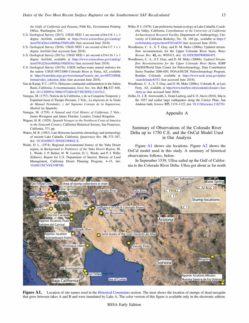
Figure A1 shows site locations. Figure A2 shows theOxCal model used in this study. A summary of historicalobservations follows, below.

In September 1539, Ulloa sailed up the Gulf of Califor-nia to the Colorado River Delta. Ulloa got about as far north

Figure A1. Location of site names used in the Historical Constraints section. The inset shows the location of stumps of dead mesquitethat grew between lakes A and B and were inundated by Lake A. The color version of this figure is available only in the electronic edition.

Dates of the Two Most Recent Surface Ruptures on the Southernmost SAF Recalculated 13

BSSA Early Edition

as present-day Montague Island, at the southern edge of theDelta, but that was not northward enough to determinewhether the full Colorado River was flowing southward intothe Gulf. He described the sea there as “reddish and turned tomud,” as if the Colorado River was actively dumping sedi-ment nearby, yet the channels he attempted to navigate wereentirely tidal and were left dry at low tide (Ulloa, in Wagner,1929, p. 20). This was no different from conditions there inthe nineteenth and twentieth centuries, where a tidal rangeapproaching 10 m creates strong currents and a tidal boreexceeding 1 m during spring tides (United States Hydro-graphic Office, 1918, pp. 155–157). In the end, Ulloa aban-doned his northward journey near Montague Island becausehis boats could not go further.

In 1540, Alarcón sailed up the Gulf of California, in anattempt to extend Ulloa’s exploration northward. By August,Alarcón reached the shoals where Ulloa had turned back, butAlarcón pushed onward. Eventually, with much difficulty,his crew “found a mighty river with such a furious currentthat [they] could scarcely sail against it” (Alarcón, in Ham-mond and Rey, 1940, pp. 125–126). Determining the up-stream extent of Alarcón’s journey has been an elusivetask ever since; Alarcón described reaching “some very highmountains among which the river flowed in a narrow can-yon” (Alarcón, in Hammond and Rey, 1940, p. 153), whichwould imply he had passed the confluence of the Gilaand Colorado Rivers above present-day Yuma, but other es-timates suggest a shorter upstream traverse (Alarcón, inHammond and Rey, 1940, p. 154; Pedro de Castañeda, inHammond and Rey, 1940, p. 211; Bancroft, 1884, p. 93).Regardless, it is clear that in 1540 the Colorado River hadstrong currents to the Gulf of California, indicating that LakeCahuilla was not filling at that time.

In 1604 and 1605, Oñate and Escobar explored overlandwestward from New Mexico, following the Bill WilliamsRiver to the Colorado River at present-day Lake Havasu;from there, they followed the Colorado River downstreampast the Gila River (Bolton, 1919a, pp. 27–32). Below theconfluence with the Gila River, Escobar estimated that theriver continued 20 leagues (∼110 km) to the sea and that“the river bottom appeared wider [and] the river has somebranches which all the year carry water” (Escobar, in Bolton,1919a, pp. 32–33). They reached the Cocapa settlement that“extends to the sea, or to the place reached by the salt water,which enters the river from the sea some four or five leagues”(Escobar, in Bolton, 1919a, p. 33) before continuing to Mon-tague Island and the Gulf of California (Bolton, 1916,pp. 276–278; Bolton, 1919a, pp. 34–35). In January 1605,as in 1540, the Colorado River was clearly flowing to theGulf of California.

In 1687, Kino founded Mission Nuestra Señora de losDolores in what is now the inland parts of Sonora, Mexico,south of Nogales; he continued to live there for the next24 yrs, until his death. In 1700, Kino explored the Gila Rivervalley westward to its confluence with the Colorado River.He climbed two hills just east of the confluence (likely in the

Gila Mountains), from which he could see that “the two riv-ers, below the confluence, ran united about ten leagues to thewest, and then, turning southward, about twenty leaguesfarther on emptied into the head of the Sea of California”(Kino, in Bolton, 1919b, Vol. 1, pp. 249, 253). He alsosaw “a large stretch of country in California” (Kino, in Bol-ton, 1919b, Vol. 1, p. 253), but it is unclear whether he wouldhave climbed high enough to be able to see a full Lake Ca-huilla, had it existed at the time. Nonetheless, Kino made nonotes of reports or descriptions of a lake in the Salton trough.

Figure A2. OxCal model used to calculate the ages of lakes Aand B. The color version of this figure is available only in the elec-tronic edition.

14 T. K. Rockwell, A. J. Meltzner, and E. C. Haaker

BSSA Early Edition

In 1701, Kino returned to the confluence of the Gila andColorado Rivers and continued onward, following the rivermore than 18 leagues (∼100 km) toward the Gulf of Califor-nia. There, Kino crossed the river on a raft, and he describedthe river as “very large volumed” and “about two hundredvaras [∼170 m] wide,” noting that people “did not touchthe bottom except at the two banks” (Kino, in Bolton,1919b, Vol. 1, p. 316). The next year, Kino returned tothe Colorado River near where it “empties into the headof the Sea of California.” There, he again described the riveras “very large volumed and very wide” and difficult to cross(Kino, in Bolton, 1919b, Vol. 1, pp. 341–344).

In 1706, Fray Manuel de Oyuela traveled with Kino andclimbed the highest of the Pinacate Peaks. From there,Oyuela could see as far as the Gulf of California, and he de-scribed “the very large volumed Rio Colorado which entersinto the sea” at the head of the Gulf (Oyuela, in Bolton,1919b, Vol. 2, p. 212). During all of Kino’s visits to the Colo-rado Delta, from 1700 to 1706, it is clear that the ColoradoRiver was flowing to the Gulf of California.

One driving question of Kino’s expeditions was deter-mining whether California was a peninsula or an island.At one point in 1702, Kino acknowledges in his diary thatthere were reports of a body of water northwest of the Colo-rado Delta, but he summarily dismisses those reports as de-scribing the Pacific Ocean: “if some hostile and obstinatepersons should maintain that some Quiquima Indians saythat farther west the sea still extends to the northwest, theseQuiquima speak of the other sea, on the opposite coast, andnot of this our Sea of California…” (Kino, in Bolton, 1919b,Vol. 1, p. 354). Thus, it is possible that some water may havebeen present in the Salton trough between 1700 and 1706,but the Colorado River was clearly flowing into the Gulfat that time.

In 1721, Ugarte sailed up the Gulf of California to themouth of the Colorado River but, like Ulloa 182 yrs earlier,was unable to pass through the shoals, where there werestrong, tidally driven currents (Venegas, 1759, Vol. 2,pp. 56–58). Ugarte proceeded to Montague Island, wherehe observed that the river “ejected into the sea grass, leaves,weeds, trunks of trees, burnt logs, the timbers of cottages andthe like” (Venegas, 1759, Vol. 2, p. 59). While this would beconsistent with a full-flowing Colorado River emptying intothe Gulf, Ugarte also noted that “on the two preceding nightsthe weather had been very tempestuous with thunders andlightnings and violent rains, which had occasioned thetwo inundations they had observed in the river” (Venegas,1759, Vol. 2, p. 59). Our assessment, therefore, is that theevidence is inconclusive as to whether the full ColoradoRiver was flowing to the Gulf in 1721.

In 1746, Consag sailed up the Gulf of California to themouth of the Colorado River, where he described similarchallenges with the tides as the previous explorers; hereached Montague Island but was unable to travel much fur-ther upstream due to strong tidal currents (Consag, in Ven-egas, 1759, Vol. 2, pp. 342–349). Meanwhile, Consag’s crew

explored limited distances overland by foot: they spent a dayand a half looking for drinking water near a place they calledSan Buenaventura (∼10 km north of present-day San Felipe,Baja California; see map of Consag, in original Spanish textof Venegas, 1757, Vol. 3, after p. 194), and they briefly ex-plored the land near Montague Island (Consag, in Venegas,1759, Vol. 2, pp. 346, 348). Again, the evidence is inconclu-sive as to whether the full Colorado River was flowing to theGulf of California in 1746. Furthermore, it appears Consagdid not reach a place where he could have seen a lake in theSalton trough, had it existed at the time.

Father Sedelmair explored the region of the Gila andColorado Rivers on several expeditions between 1744 and1750. In 1744, he explored both rivers upstream of their con-fluence but did not explore downstream (Venegas, 1759, Vol.2, pp. 181–185; Bancroft, 1884, pp. 536–537; Sedelmair, inDunne, 1955, pp. 15–53). Sedelmair returned to the region inOctober and November 1748, although he oddly reported thedates of that trip as being in October and November 1749;regardless, he explored only a short distance downstream ofthe confluence of the Colorado and Gila Rivers (Sedelmair,1750; Venegas, 1759, Vol. 2, pp. 209–210; Bancroft, 1884,p. 540; Dunne, 1955, pp. 55–66). Finally, in 1750, Sedelmairwent farther downstream, to a point west of the sand dunes ofthe Gran Desierto de Altar, apparently almost reaching theGulf of California (Bancroft, 1884, pp. 540–541; Dunne,1955, pp. 67–75).

Appendix B

Online Access to Historical Accounts

Some historical accounts consulted in this study areavailable online:

Sedelmair (1750):https://books.google.com/books?id=HJgEAAAAQAAJhttp://cdigital.dgb.uanl.mx/la/1080023894_C/1080023

894_T1/1080023894_MA.PDFhttp://cdigital.dgb.uanl.mx/la/1080023894_C/1080023

894_T1/1080023894_03.pdf

Venegas (1757):Volume 1: https://archive.org/details/cihm_18688Volume 2: https://archive.org/details/cihm_18689Volume 3: https://archive.org/details/cihm_18690All: https://catalog.hathitrust.org/Record/100258713

Venegas (1759):Volume 1: https://archive.org/details/naturalcivilhist01veneVolume 2: https://archive.org/details/naturalcivilhist02veneAll: https://catalog.hathitrust.org/Record/100268375

Bancroft (1884):https://archive.org/details/thenorthmexivol115bancmisshttps://archive.org/details/worksofhuberthow15bancrich

Dates of the Two Most Recent Surface Ruptures on the Southernmost SAF Recalculated 15

BSSA Early Edition

https://archive.org/details/historynorthmex02nemogooghttps://archive.org/details/historynorthmex03nemogooghttps://archive.org/details/annalsofspanishn01oakhrich

Blake (1915):https://archive.org/details/imperialvalleya00blakgoog

Cory (1915):https://archive.org/details/imperialvalleya00blakgoog

Bolton (1916):https://archive.org/details/spanishexplorati00bolthttps://archive.org/details/spanishexplorat03boltgoog

Bolton (1917):https://archive.org/details/pacificoceaninhi00panaialahttps://archive.org/details/pacificoceaninhi00panauoft

Bolton (1919a):http://www.jstor.org/stable/25011616https://archive.org/details/fatherescobarsre00boltrich

Bolton (1919b):Volume 1: https://archive.org/details/kinoshistoricalm00

kinoVolume 2: https://archive.org/details/kinoshistoricalm02

kinouoft

Bolton (1930):Volume 1: https://archive.org/details/anzascaliforniae01

boltVolume 2: https://archive.org/details/anzascaliforniae02

boltVolume 3: https://archive.org/details/anzascaliforniae03

boltVolume 4: https://archive.org/details/anzascaliforniae04

bolt

Volume 5: https://archive.org/details/anzascaliforniae05bolt

Dunne (1955):https://catalog.hathitrust.org/Record/001652279

United States Hydrographic Office (1918):https://archive.org/details/mexicoandcentra00offigoog

Kohler et al. (1959):https://catalog.hathitrust.org/Record/101740906http://www.nws.noaa.gov/oh/hdsc/Technical_papers/TP

37.pdf

All websites were last accessed on June 2018.

Department of Geological SciencesSan Diego State UniversitySan Diego, California 92182trockwell@mail.sdsu.edu

(T.K.R.)

Earth Observatory of SingaporeNanyang Technological University50 Nanyang AvenueSingapore 639798Singaporemeltzner@ntu.edu.sg

(A.J.M.)

G3SoilWorks, Inc.350 Fischer Avenue FrontCosta Mesa, California 92626ehaaker@g3soilworks.com

(E.C.H.)

Manuscript received 28 December 2017;Published Online 17 July 2018

16 T. K. Rockwell, A. J. Meltzner, and E. C. Haaker

BSSA Early Edition