Embed Size (px)
Citation preview

Decomposing MWR - An Update
Date: 20th April 2010Produced by: Dr. Stefan J. Illmer,
Head of Investment Reporting
Produced by: Dr. Stefan J. Illmer, Investment ReportingDate: 20th April 2010 Slide 2
IntroductionCalculation of MWRContribution to MWRMWR-AttributionProfit and Loss AttributionHypothetical ExampleSimple Example for an IRR ImplementationComments and QuestionsReferences
Agenda

Produced by: Dr. Stefan J. Illmer, Investment ReportingDate: 20th April 2010 Slide 3
Introduction
Produced by: Dr. Stefan J. Illmer, Investment ReportingDate: 20th April 2010 Slide 4
Money-weighted rate of return (MWR) measures the return of a portfolio in a way that the return is sensitive to changes in the money invested:
MWR measures the return from a client’s perspective where he does have control over the (external) cash flows.MWR does not allow a comparison across peer groups.MWR does allow a comparison against a benchmark (adjusted for cash flows).MWR is best measured by the internal rate of return (IRR).calculating, decomposing and reporting MWRs is not commonpractice.MWRs are not generally covered by the GIPS Standards - just for private equity and closed end real estate funds.
Initial comments on MWR
Produced by: Dr. Stefan J. Illmer, Investment ReportingDate: 20th April 2010 Slide 5
The MWR allows a decomposition of the portfolio return reflecting the client’s main investment decision:
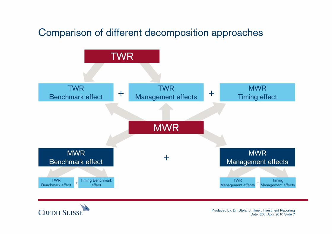
TWR Benchmark effect => reflects the return contribution based on the client’s decision to invest his initial capital into a specific benchmark strategy (corresponds to the TWR benchmark return).TWR Management effect => reflects the return contribution based on deviating from the benchmark strategy by asset allocation andstock picking (corresponds to the TWR attribution effects).MWR Timing effect => reflects the return contribution of changing the initial invested capital into the benchmark strategy and into the asset allocation of the portfolio (corresponds to the differencebetween MWR and TWR).
Decomposition of MWR versus TWR
Produced by: Dr. Stefan J. Illmer, Investment ReportingDate: 20th April 2010 Slide 6
The MWR allows also a decomposition of the portfolio return without explicitly separating the timing effect:
MWR Benchmark effect => reflects the return contribution based on the client’s decision to invest his capital into a specific benchmark strategy (including the effect of changing the initialinvested capital).MWR Management effect => reflects the return contribution based on deviating from the benchmark strategy by asset allocation and stock picking (including the effect of changing the initial invested capital).
Decomposition of MWR - another perspective
Produced by: Dr. Stefan J. Illmer, Investment ReportingDate: 20th April 2010 Slide 7
Comparison of different decomposition approaches
TWRBenchmark effect
TWRManagement effects
MWRTiming effect
MWRBenchmark effect
MWRManagement effects
TWR
MWR
+ +
+
TWRBenchmark effect
TWRManagement effects
TWRManagement effects
TimingManagement effects
Timing Benchmark effect
+ +
Produced by: Dr. Stefan J. Illmer, Investment ReportingDate: 20th April 2010 Slide 8
Calculation of MWR
Produced by: Dr. Stefan J. Illmer, Investment ReportingDate: 20th April 2010 Slide 9
Calculation of the MWR for the portfolio.Calculation of the MWR for the benchmark=> by simulating the portfolio's cash in- and outflows also for the
benchmark.Calculation of the excess MWR.
First step towards MWR-Attribution
Produced by: Dr. Stefan J. Illmer, Investment ReportingDate: 20th April 2010 Slide 10
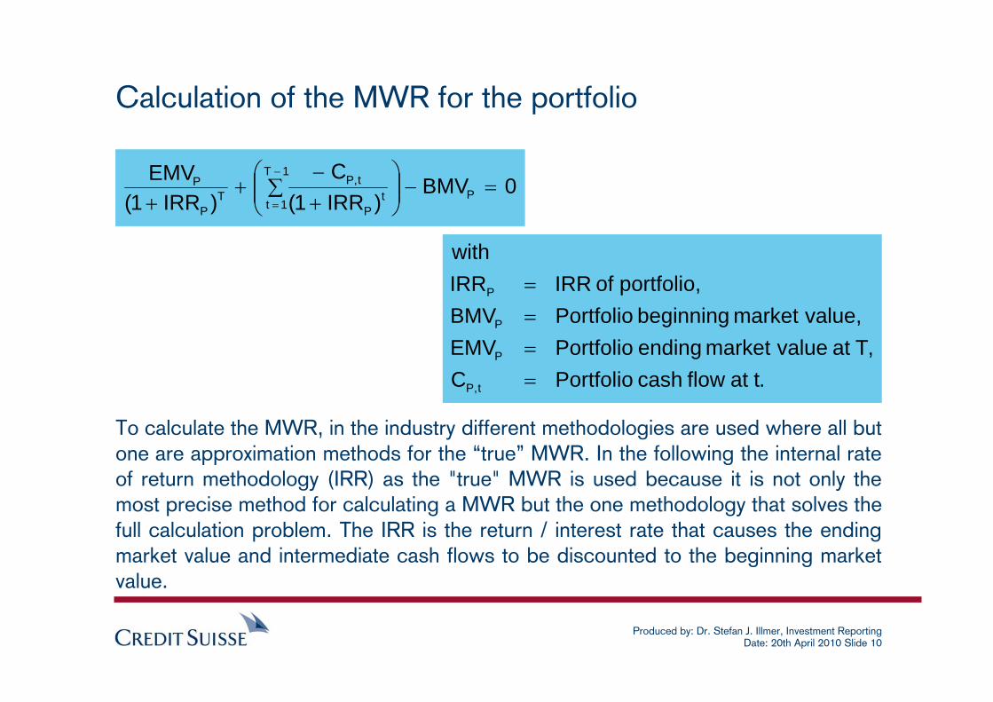
Calculation of the MWR for the portfolio
0BMV)IRR1(
C)IRR1(
EMVP
1T
1tt
P
t,PT
P
P =−⎟⎟⎠
⎞⎜⎜⎝
⎛∑
+−
++
−
=
.t atflow cash PortfolioC,T at value market ending PortfolioEMV
value, market beginning PortfolioBMVportfolio, of IRRIRR
with
t,P
P
P
P
====
To calculate the MWR, in the industry different methodologies are used where all but one are approximation methods for the “true” MWR. In the following the internal rate of return methodology (IRR) as the "true" MWR is used because it is not only the most precise method for calculating a MWR but the one methodology that solves the full calculation problem. The IRR is the return / interest rate that causes the ending market value and intermediate cash flows to be discounted to the beginning market value.
Produced by: Dr. Stefan J. Illmer, Investment ReportingDate: 20th April 2010 Slide 11
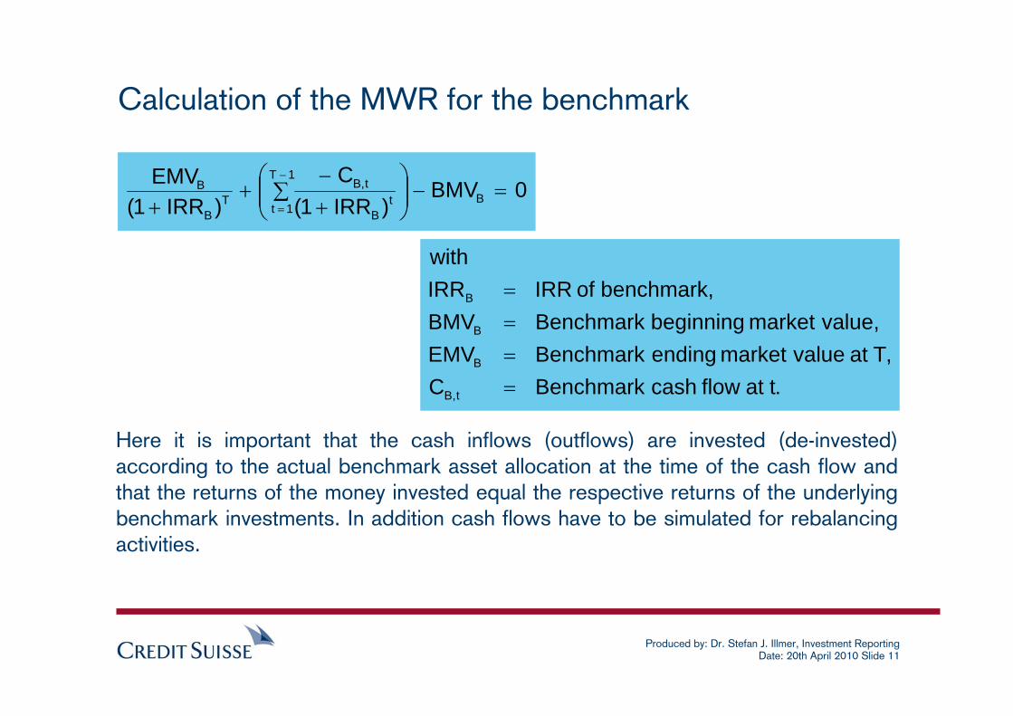
Calculation of the MWR for the benchmark
0BMV)IRR1(
C)IRR1(
EMVB
1T
1tt
B
t,BT
B
B =−⎟⎟⎠
⎞⎜⎜⎝
⎛∑
+−
++
−
=
.t atflow cash BenchmarkC,T at value market ending BenchmarkEMV
value, market beginning BenchmarkBMVbenchmark, of IRRIRR
with
t,B
B
B
B
====
Here it is important that the cash inflows (outflows) are invested (de-invested) according to the actual benchmark asset allocation at the time of the cash flow and that the returns of the money invested equal the respective returns of the underlying benchmark investments. In addition cash flows have to be simulated for rebalancing activities.
Produced by: Dr. Stefan J. Illmer, Investment ReportingDate: 20th April 2010 Slide 12
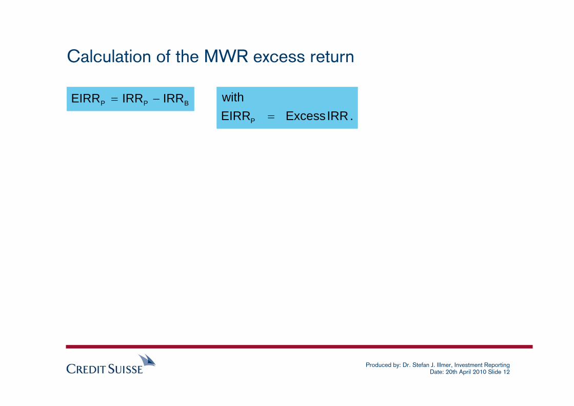
Calculation of the MWR excess return
BPP IRRIRREIRR −=.IRR ExcessEIRR
with
P =
Produced by: Dr. Stefan J. Illmer, Investment ReportingDate: 20th April 2010 Slide 13
Contribution to MWR
Produced by: Dr. Stefan J. Illmer, Investment ReportingDate: 20th April 2010 Slide 14
Calculation of the profit and loss of the different asset classes.Calculation of the average invested capital for the different asset classes.Calculation of the asset class contribution to the MWR for the portfolio.Calculation of the asset class contribution to the MWR for the benchmark.Calculation of the asset class contribution to the excess MWR.
Second step towards MWR-Attribution
Produced by: Dr. Stefan J. Illmer, Investment ReportingDate: 20th April 2010 Slide 15
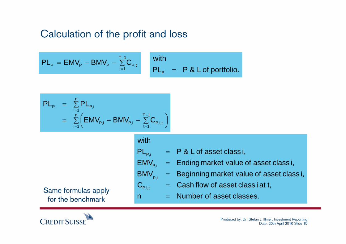
Calculation of the profit and loss
∑−−=−
=
1T
1tt,PPPP CBMVEMVPL
portfolio. of L&PPLwith
P =
∑ ⎟⎠⎞⎜
⎝⎛ ∑−−=
∑=
=
−
=
=n
1i
1T
1tt,i,Pi,Pi,P
n
1ii,PP
CBMVEMV
PLPL
classes. asset of Numbern t, at i class asset offlow CashC
i, class asset of value market BeginningBMVi, class asset of value market EndingEMV
i, class asset of L&PPLwith
t,i,P
i,P
i,P
i,P
=====
Same formulas apply for the benchmark
Produced by: Dr. Stefan J. Illmer, Investment ReportingDate: 20th April 2010 Slide 16
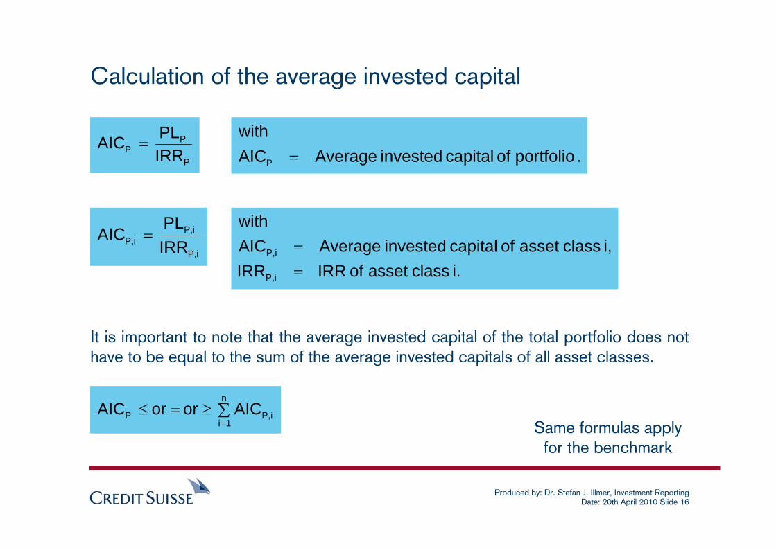
Calculation of the average invested capital
P
PP IRR
PLAIC =.portfolio of capital invested AverageAIC
with
P =
i,P
i,Pi,P IRR
PLAIC =
i. class asset of IRRIRRi, class asset of capital invested AverageAIC
with
i,P
i,P
==
∑≥=≤=
n
1ii,PP AICororAIC
It is important to note that the average invested capital of the total portfolio does not have to be equal to the sum of the average invested capitals of all asset classes.
Same formulas apply for the benchmark
Produced by: Dr. Stefan J. Illmer, Investment ReportingDate: 20th April 2010 Slide 17
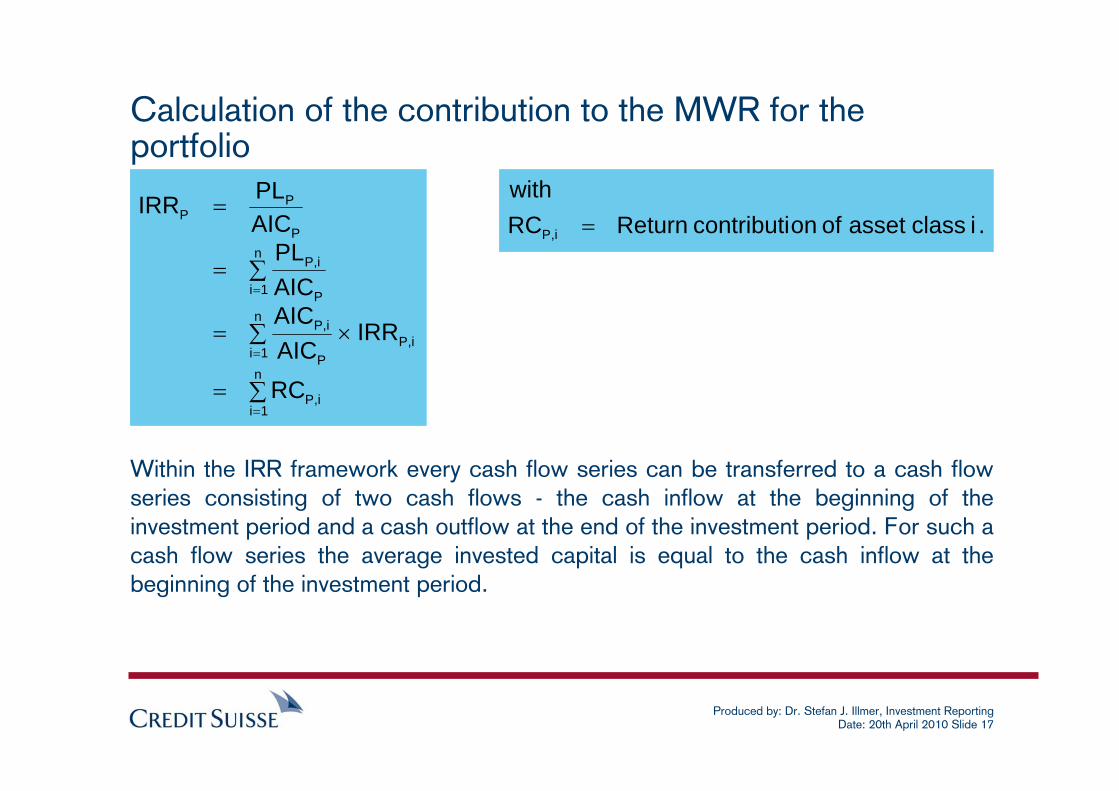
Calculation of the contribution to the MWR for the portfolio
∑=
∑ ×=
∑=
=
=
=
=
n
1ii,P
n
1ii,P
P
i,P
n
1i P
i,P
P
PP
RC
IRRAICAICAICPL
AICPLIRR
.i class asset of oncontributi ReturnRCwith
i,P =
Within the IRR framework every cash flow series can be transferred to a cash flow series consisting of two cash flows - the cash inflow at the beginning of the investment period and a cash outflow at the end of the investment period. For such a cash flow series the average invested capital is equal to the cash inflow at the beginning of the investment period.
Produced by: Dr. Stefan J. Illmer, Investment ReportingDate: 20th April 2010 Slide 18
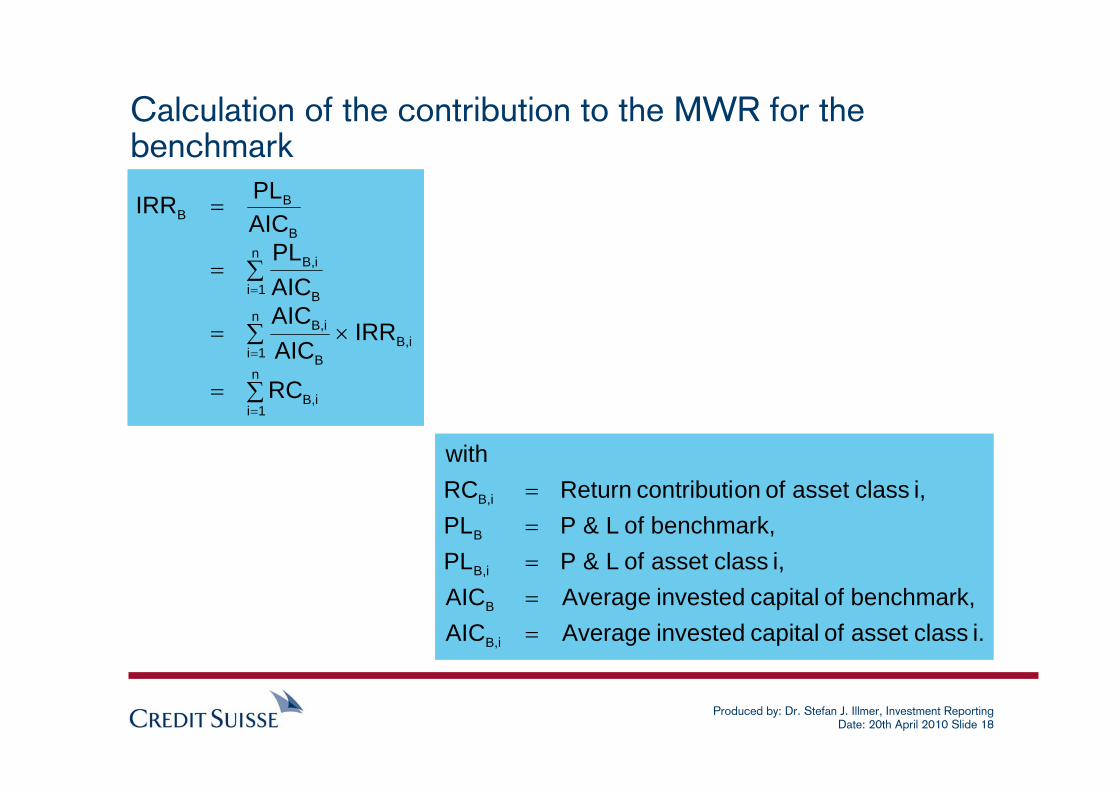
Calculation of the contribution to the MWR for the benchmark
∑=
∑ ×=
∑=
=
=
=
=
n
1ii,B
n
1ii,B
B
i,B
n
1i B
i,B
B
BB
RC
IRRAICAICAICPL
AICPLIRR
i. class asset of capital invested AverageAICbenchmark, of capital invested AverageAIC
i, class asset of L&PPLbenchmark, of L&PPL
i, class asset of oncontributi ReturnRCwith
iB,
B
i,B
B
i,B
=====
Produced by: Dr. Stefan J. Illmer, Investment ReportingDate: 20th April 2010 Slide 19
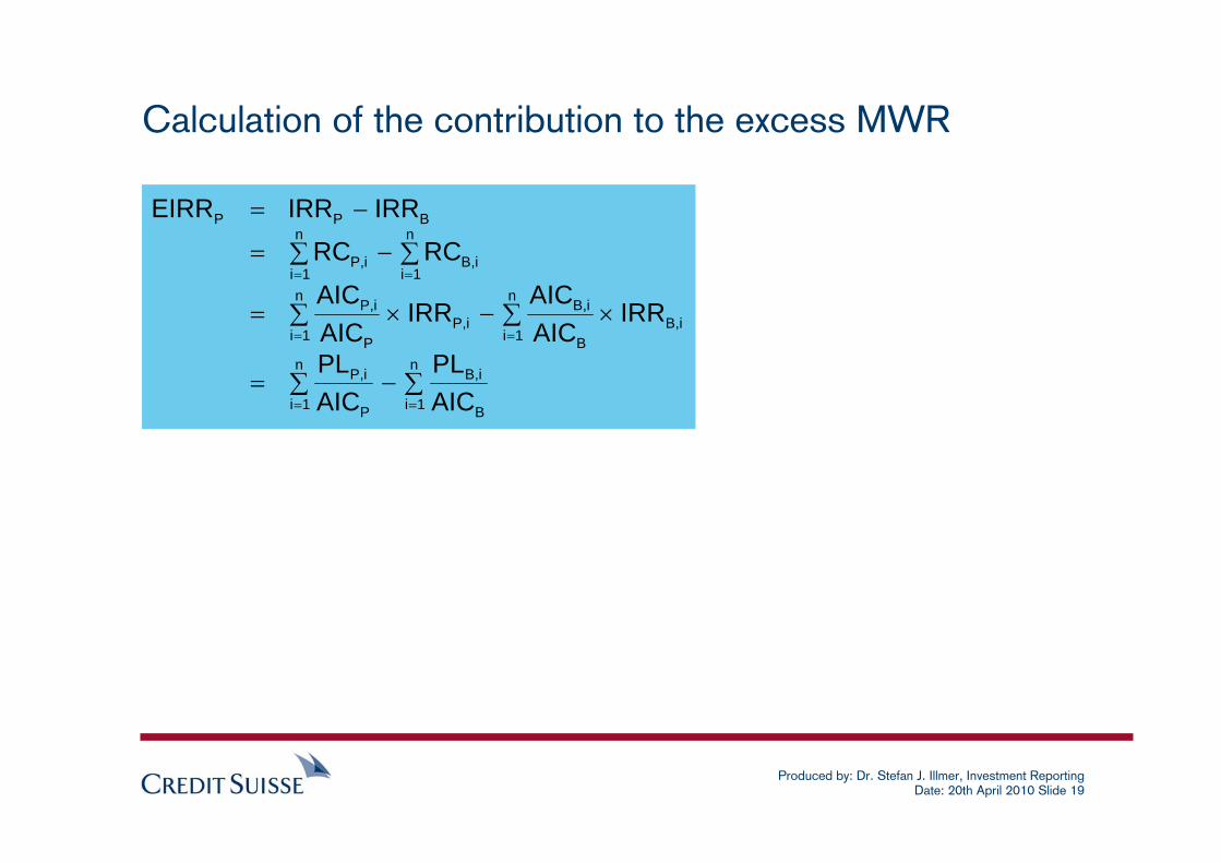
Calculation of the contribution to the excess MWR
∑−∑=
∑ ×−∑ ×=
∑−∑=
−=
==
==
==
n
1i B
i,Bn
1i P
i,P
n
1ii,B
B
i,Bn
1ii,P
P
i,P
n
1ii,B
n
1ii,P
BPP
AICPL
AICPL
IRRAICAIC
IRRAICAIC
RCRCIRRIRREIRR
Produced by: Dr. Stefan J. Illmer, Investment ReportingDate: 20th April 2010 Slide 20
MWR-Attribution
Produced by: Dr. Stefan J. Illmer, Investment ReportingDate: 20th April 2010 Slide 21
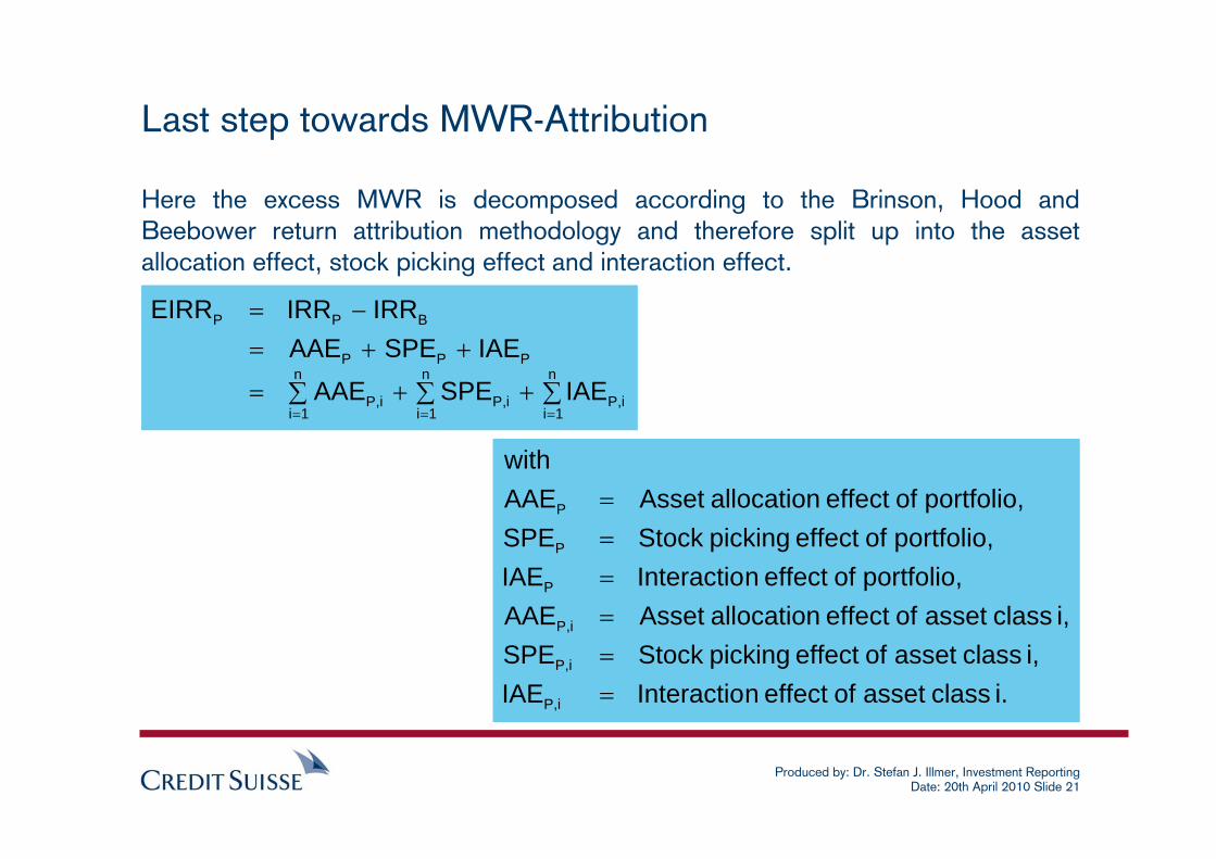
Here the excess MWR is decomposed according to the Brinson, Hood and Beebower return attribution methodology and therefore split up into the asset allocation effect, stock picking effect and interaction effect.
Last step towards MWR-Attribution
∑ ∑ ∑++=
++=−=
= = =
n
1i
n
1i
n
1ii,Pi,Pi,P
PPP
BPP
IAESPEAAEIAESPEAAE
IRRIRREIRR
i. class asset of effect nInteractioIAEi, class asset of effect picking StockSPE
i, class asset of effect allocation AssetAAEportfolio, of effect nInteractioIAE
portfolio, of effect picking StockSPEportfolio, of effect allocation AssetAAE
with
i,P
i,P
i,P
P
P
P
======
Produced by: Dr. Stefan J. Illmer, Investment ReportingDate: 20th April 2010 Slide 22
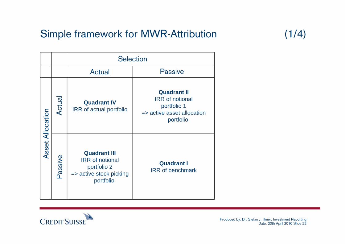
Simple framework for MWR-Attribution (1/4)
Quadrant IIRR of benchmark
Quadrant IIIIRR of notional
portfolio 2=> active stock picking
portfolio
Quadrant IIIRR of notional
portfolio 1=> active asset allocation
portfolio
Quadrant IVIRR of actual portfolio
Ass
et A
lloca
tion
SelectionA
ctua
lP
assi
ve
Actual Passive
Produced by: Dr. Stefan J. Illmer, Investment ReportingDate: 20th April 2010 Slide 23
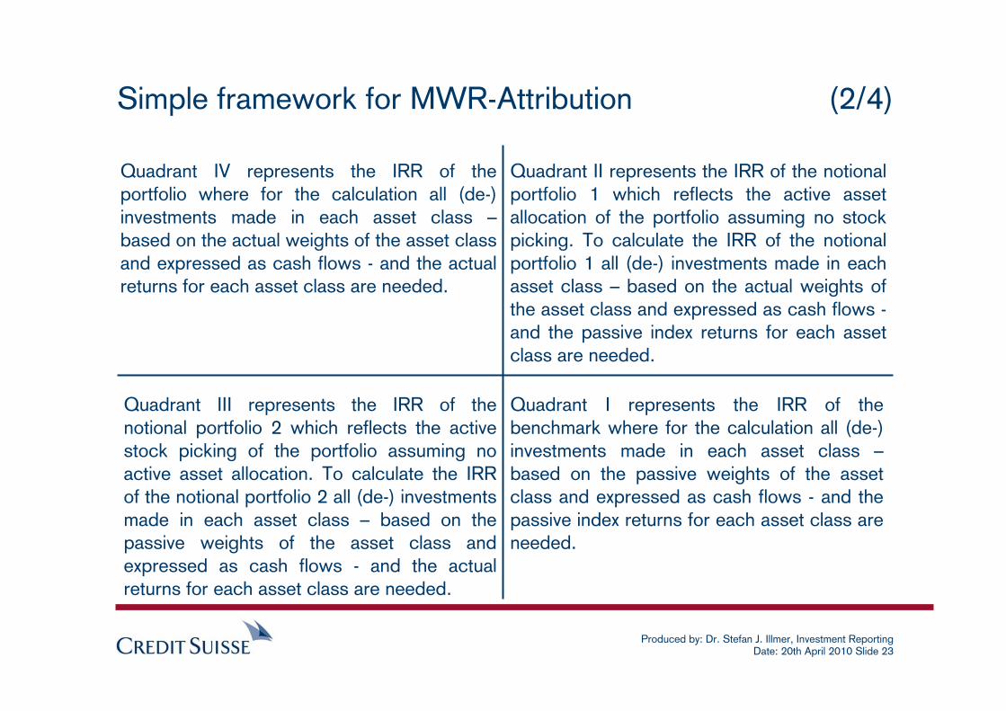
Quadrant I represents the IRR of the benchmark where for the calculation all (de-) investments made in each asset class –based on the passive weights of the asset class and expressed as cash flows - and the passive index returns for each asset class are needed.
Simple framework for MWR-Attribution (2/4)
Quadrant II represents the IRR of the notional portfolio 1 which reflects the active asset allocation of the portfolio assuming no stock picking. To calculate the IRR of the notional portfolio 1 all (de-) investments made in each asset class – based on the actual weights of the asset class and expressed as cash flows -and the passive index returns for each asset class are needed.
Quadrant III represents the IRR of the notional portfolio 2 which reflects the active stock picking of the portfolio assuming no active asset allocation. To calculate the IRR of the notional portfolio 2 all (de-) investments made in each asset class – based on the passive weights of the asset class and expressed as cash flows - and the actual returns for each asset class are needed.
Quadrant IV represents the IRR of the portfolio where for the calculation all (de-) investments made in each asset class –based on the actual weights of the asset class and expressed as cash flows - and the actual returns for each asset class are needed.
Produced by: Dr. Stefan J. Illmer, Investment ReportingDate: 20th April 2010 Slide 24
Simple framework for MWR-Attribution (3/4)
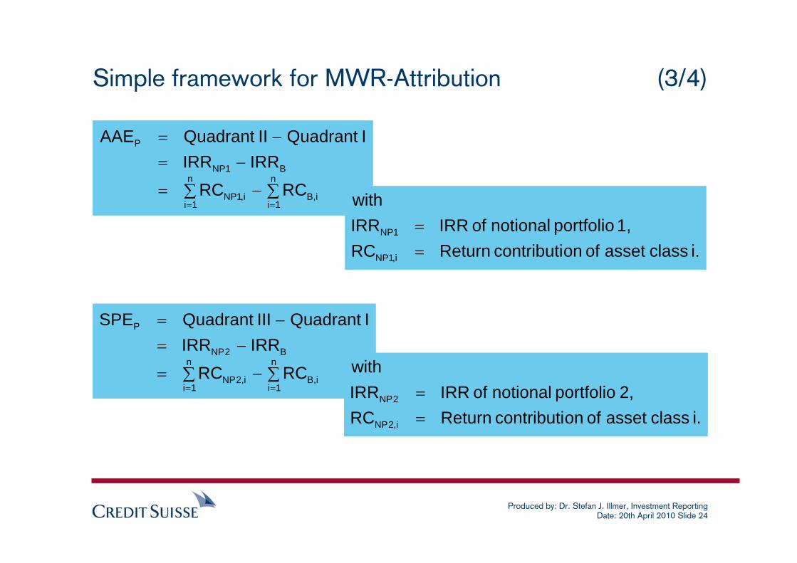
∑ ∑−=
−=−=
= =
n
1i
n
1ii,Bi,1NP
B1NP
P
RCRCIRRIRR
I QuadrantII QuadrantAAE
i. class asset of oncontributi ReturnRC1, portfolio notional of IRRIRR
with
i,1NP
1NP
==
∑ ∑−=
−=−=
= =
n
1i
n
1ii,Bi,2NP
B2NP
P
RCRCIRRIRR
I QuadrantIII QuadrantSPE
i. class asset of oncontributi ReturnRC2, portfolio notional of IRRIRR
with
i,2NP
2NP
==
Produced by: Dr. Stefan J. Illmer, Investment ReportingDate: 20th April 2010 Slide 25
Simple framework for MWR-Attribution (4/4)
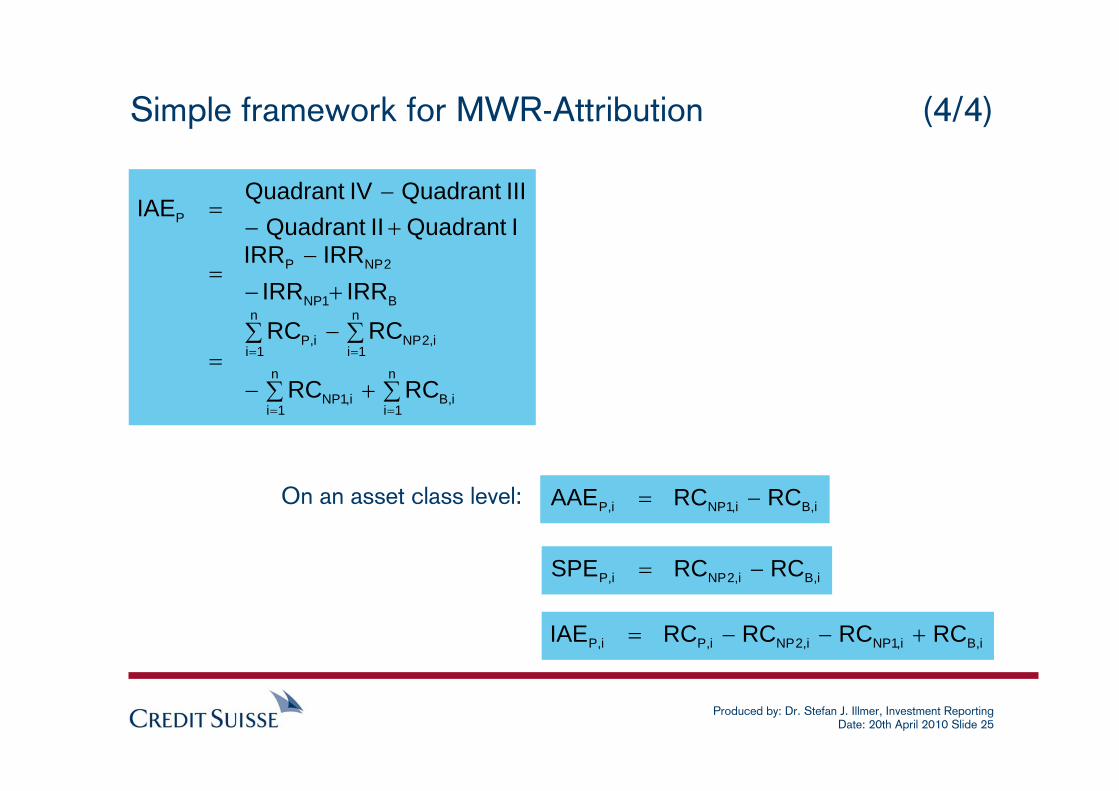
∑+∑−
∑ ∑−=
+−
−=
+−−
=
==
= =
n
1ii,B
n
1ii,1NP
n
1i
n
1ii,2NPi,P
B1NP
2NPP
P
RCRC
RCRCIRRIRR
IRRIRRI Quadrant II QuadrantIII QuadrantIV Quadrant
IAE
i,Bi,1NPi,P RCRCAAE −=
i,Bi,2NPi,P RCRCSPE −=
i,Bi,1NPi,2NPi,Pi,P RCRCRCRCIAE +−−=
On an asset class level:
Produced by: Dr. Stefan J. Illmer, Investment ReportingDate: 20th April 2010 Slide 26
Profit and Loss Attribution
Produced by: Dr. Stefan J. Illmer, Investment ReportingDate: 20th April 2010 Slide 27
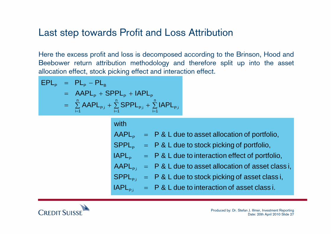
Here the excess profit and loss is decomposed according to the Brinson, Hood and Beebower return attribution methodology and therefore split up into the asset allocation effect, stock picking effect and interaction effect.
Last step towards Profit and Loss Attribution
∑ ∑ ∑++=
++=−=
= = =
n
1i
n
1i
n
1ii,Pi,Pi,P
PPP
BPP
IAPLSPPLAAPLIAPLSPPLAAPL
PLPLEPL
i. class asset of ninteractio to due L&PIAPLi, class asset of picking stock to due L&PSPPL
i, class asset of allocation asset to due L&PAAPLportfolio, of effect ninteractio to due L&PIAPL
portfolio, of picking stock to due L&PSPPLportfolio, of allocation asset to due L&PAAPL
with
i,P
i,P
i,P
P
P
P
======
Produced by: Dr. Stefan J. Illmer, Investment ReportingDate: 20th April 2010 Slide 28
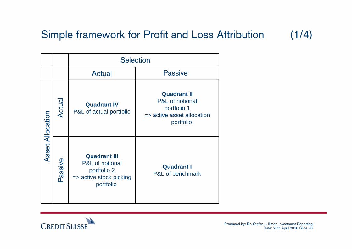
Simple framework for Profit and Loss Attribution (1/4)
Quadrant IP&L of benchmark
Quadrant IIIP&L of notional
portfolio 2=> active stock picking
portfolio
Quadrant IIP&L of notional
portfolio 1=> active asset allocation
portfolio
Quadrant IVP&L of actual portfolio
Ass
et A
lloca
tion
SelectionA
ctua
lP
assi
ve
Actual Passive
Produced by: Dr. Stefan J. Illmer, Investment ReportingDate: 20th April 2010 Slide 29
Quadrant I represents the P&L of the benchmark where for the calculation all (de-) investments made in each asset class –based on the passive weights of the asset class and expressed as cash flows - and the passive index returns for each asset class are needed.
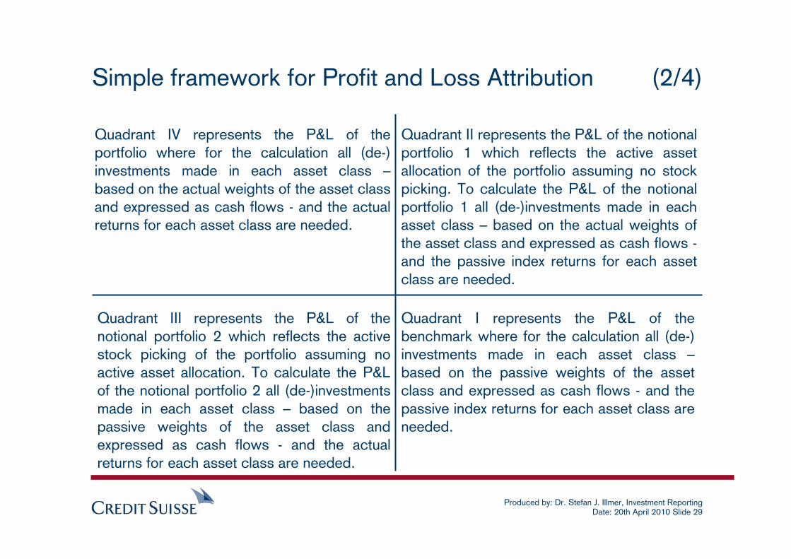
Simple framework for Profit and Loss Attribution (2/4)
Quadrant II represents the P&L of the notional portfolio 1 which reflects the active asset allocation of the portfolio assuming no stock picking. To calculate the P&L of the notional portfolio 1 all (de-)investments made in each asset class – based on the actual weights of the asset class and expressed as cash flows -and the passive index returns for each asset class are needed.
Quadrant III represents the P&L of the notional portfolio 2 which reflects the active stock picking of the portfolio assuming no active asset allocation. To calculate the P&L of the notional portfolio 2 all (de-)investments made in each asset class – based on the passive weights of the asset class and expressed as cash flows - and the actual returns for each asset class are needed.
Quadrant IV represents the P&L of the portfolio where for the calculation all (de-) investments made in each asset class –based on the actual weights of the asset class and expressed as cash flows - and the actual returns for each asset class are needed.
Produced by: Dr. Stefan J. Illmer, Investment ReportingDate: 20th April 2010 Slide 30
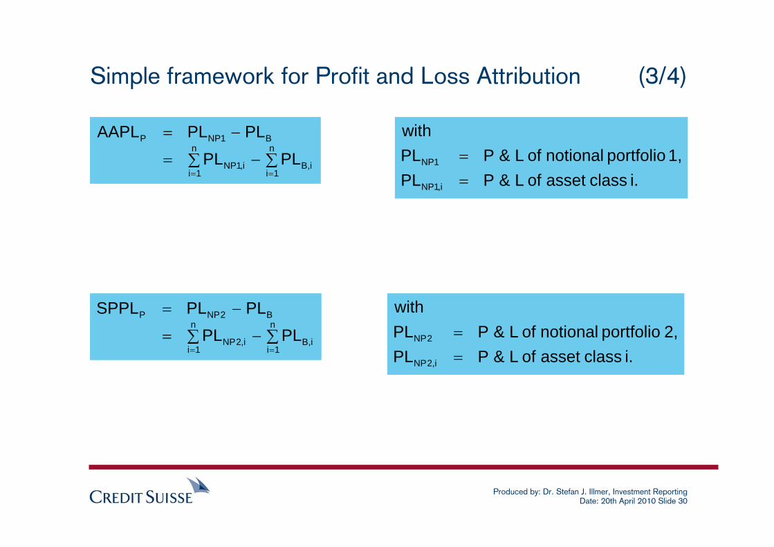
Simple framework for Profit and Loss Attribution (3/4)
∑ ∑−=
−=
= =
n
1i
n
1ii,Bi,1NP
B1NPP
PLPLPLPLAAPL
i. class asset of L&PPL1, portfolio notional of L&PPL
with
i,1NP
1NP
==
∑ ∑−=
−=
= =
n
1i
n
1ii,Bi,2NP
B2NPP
PLPLPLPLSPPL
i. class asset of L&PPL2, portfolio notional of L&PPL
with
i,2NP
2NP
==
Produced by: Dr. Stefan J. Illmer, Investment ReportingDate: 20th April 2010 Slide 31
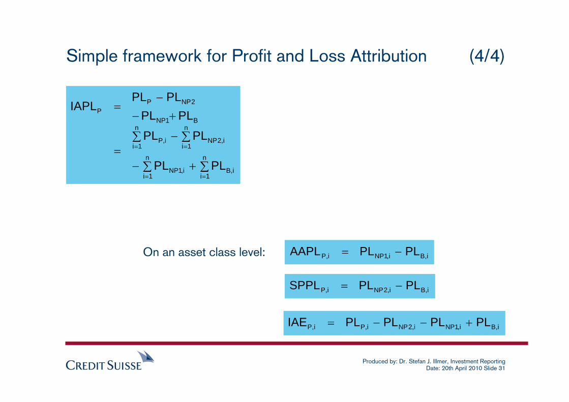
Simple framework for Profit and Loss Attribution (4/4)
On an asset class level:
∑+∑−
∑ ∑−=
+−−
=
==
= =
n
1ii,B
n
1ii,1NP
n
1i
n
1ii,2NPi,P
B1NP
2NPPP
PLPL
PLPLPLPL
PLPLIAPL
i,Bi,1NPi,P PLPLAAPL −=
i,Bi,2NPi,P PLPLSPPL −=
i,Bi,1NPi,2NPi,Pi,P PLPLPLPLIAE +−−=

Produced by: Dr. Stefan J. Illmer, Investment ReportingDate: 20th April 2010 Slide 32
Hypothetical Example
Produced by: Dr. Stefan J. Illmer, Investment ReportingDate: 20th April 2010 Slide 33
Sample multi-asset class portfolio is investing in two asset classes A and B.Relevant benchmark is also investing in these two asset classes A and B.The portfolio as well the benchmark are rebalanced on a yearly basis at the beginning of the calendar year.A two year period from 31.12.2006 until 31.12.2008 is considered.At the beginning of 2007 EUR 150 are invested in the portfolio.At the beginning of 2008 additional EUR 100 are invested into the portfolio according to the then current active asset allocation and stock pickings.
Assumptions

Produced by: Dr. Stefan J. Illmer, Investment ReportingDate: 20th April 2010 Slide 34
Return calculations (1/2)
Period 1 Period 2
Dates 31.12.2006 31.12.2007 31.12.2008
Cash flow at beginning of period
Cash flow at beginning of period
Market value at the end of period
Asset A -75.0 47.6 36.7
Asset B -75.0 -147.6 240.8
Portfolio -150.0 -100.0 277.5
Actual weights at beginning of period
Actual weights at beginning of period
Weights at the end of period
Asset A 50.0% 15.0% 13.2%
Asset B 50.0% 85.0% 86.8%
Portfolio 100.0% 100.0% 100.0%
Actual return Actual return Cummulative return
Asset A 15.0% -5.0% 17.9%
Asset B -5.0% 10.0% 12.4%
Portfolio 5.0% 7.8% 13.8%
Actual Portfolio (IRR)
Period 1 Period 2
Dates 31.12.2006 31.12.2007 31.12.2008
Cash flow at beginning of period
Cash flow at beginning of period
Market value at the end of period
Asset A -45.0 -39.5 83.0
Asset B -105.0 -60.6 167.2
Portfolio -150.0 -100.0 250.2
Passive weights at beginning of period
Passive weights at beginning of period
Weights at the end of period
Asset A 30.0% 30.0% 33.2%
Asset B 70.0% 70.0% 66.8%
Portfolio 100.0% 100.0% 100.0%
Passive return Passive return Cummulative return
Asset A -20.0% 10.0% -2.2%
Asset B 10.0% -5.0% 1.3%
Portfolio 1.0% -0.5% 0.1%
Benchmark (IRR)
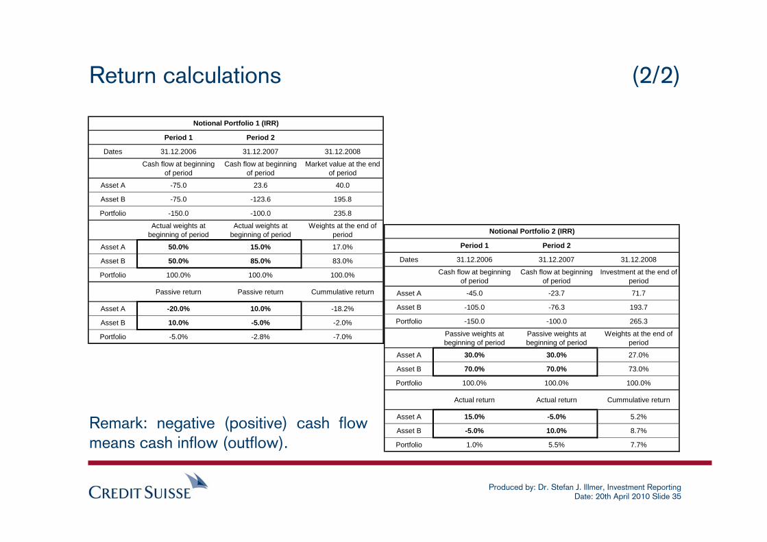
Remark: negative (positive) cash flow means cash inflow (outflow).
Produced by: Dr. Stefan J. Illmer, Investment ReportingDate: 20th April 2010 Slide 35
Period 1 Period 2
Dates 31.12.2006 31.12.2007 31.12.2008
Cash flow at beginning of period
Cash flow at beginning of period
Market value at the end of period
Asset A -75.0 23.6 40.0
Asset B -75.0 -123.6 195.8
Portfolio -150.0 -100.0 235.8
Actual weights at beginning of period
Actual weights at beginning of period
Weights at the end of period
Asset A 50.0% 15.0% 17.0%
Asset B 50.0% 85.0% 83.0%
Portfolio 100.0% 100.0% 100.0%
Passive return Passive return Cummulative return
Asset A -20.0% 10.0% -18.2%
Asset B 10.0% -5.0% -2.0%
Portfolio -5.0% -2.8% -7.0%
Notional Portfolio 1 (IRR)
Period 1 Period 2
Dates 31.12.2006 31.12.2007 31.12.2008
Cash flow at beginning of period
Cash flow at beginning of period
Investment at the end of period
Asset A -45.0 -23.7 71.7
Asset B -105.0 -76.3 193.7
Portfolio -150.0 -100.0 265.3
Passive weights at beginning of period
Passive weights at beginning of period
Weights at the end of period
Asset A 30.0% 30.0% 27.0%
Asset B 70.0% 70.0% 73.0%
Portfolio 100.0% 100.0% 100.0%
Actual return Actual return Cummulative return
Asset A 15.0% -5.0% 5.2%
Asset B -5.0% 10.0% 8.7%
Portfolio 1.0% 5.5% 7.7%
Notional Portfolio 2 (IRR)
Return calculations (2/2)
Remark: negative (positive) cash flow means cash inflow (outflow).
Produced by: Dr. Stefan J. Illmer, Investment ReportingDate: 20th April 2010 Slide 36
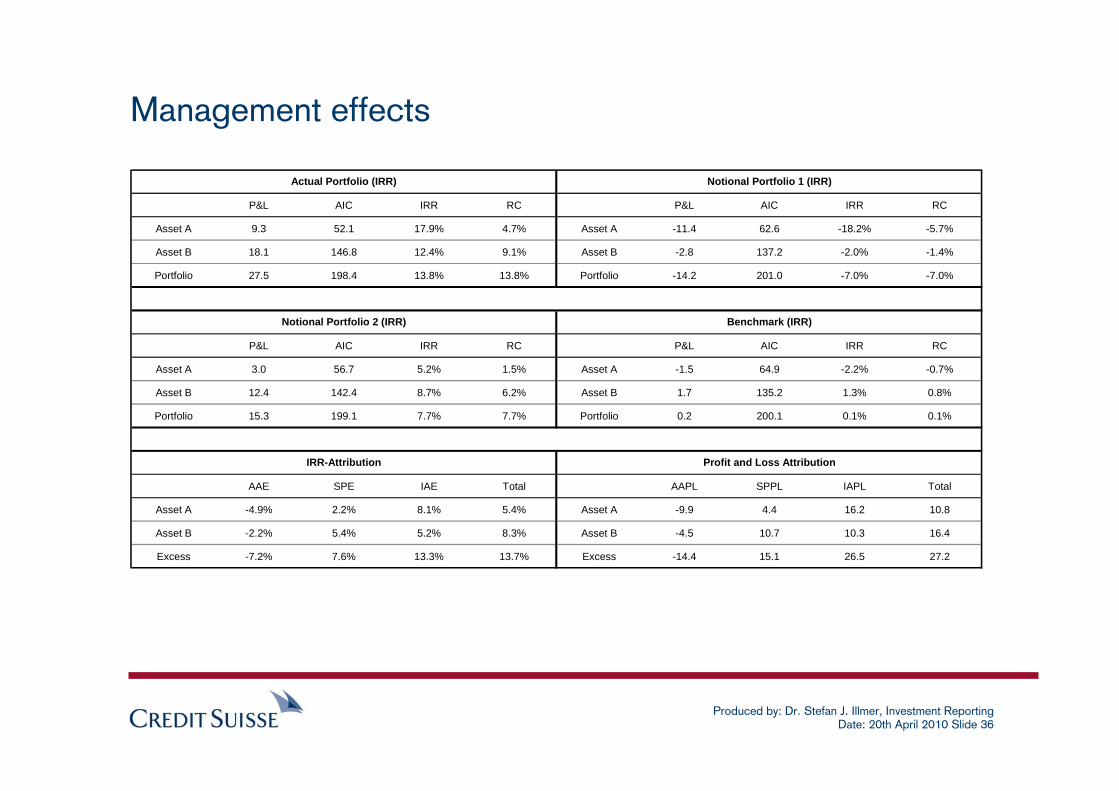
Management effects
P&L AIC IRR RC P&L AIC IRR RC
Asset A 9.3 52.1 17.9% 4.7% Asset A -11.4 62.6 -18.2% -5.7%
Asset B 18.1 146.8 12.4% 9.1% Asset B -2.8 137.2 -2.0% -1.4%
Portfolio 27.5 198.4 13.8% 13.8% Portfolio -14.2 201.0 -7.0% -7.0%
P&L AIC IRR RC P&L AIC IRR RC
Asset A 3.0 56.7 5.2% 1.5% Asset A -1.5 64.9 -2.2% -0.7%
Asset B 12.4 142.4 8.7% 6.2% Asset B 1.7 135.2 1.3% 0.8%
Portfolio 15.3 199.1 7.7% 7.7% Portfolio 0.2 200.1 0.1% 0.1%
AAE SPE IAE Total AAPL SPPL IAPL Total
Asset A -4.9% 2.2% 8.1% 5.4% Asset A -9.9 4.4 16.2 10.8
Asset B -2.2% 5.4% 5.2% 8.3% Asset B -4.5 10.7 10.3 16.4
Excess -7.2% 7.6% 13.3% 13.7% Excess -14.4 15.1 26.5 27.2
IRR-Attribution Profit and Loss Attribution
Actual Portfolio (IRR) Notional Portfolio 1 (IRR)
Notional Portfolio 2 (IRR) Benchmark (IRR)
Produced by: Dr. Stefan J. Illmer, Investment ReportingDate: 20th April 2010 Slide 37
Simple Example for an IRR Implementation
Produced by: Dr. Stefan J. Illmer, Investment ReportingDate: 20th April 2010 Slide 38
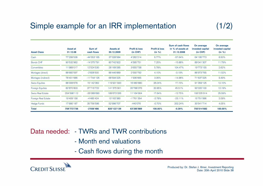
Simple example for an IRR implementation (1/2)
Asset ClassAsset at31.12.08
Sum ofcash flows
Assets at 30.12.2009
Profit & loss(in CHF)
Profit & loss(in %)
Sum of cash flows in % of assets at
31.12.2008
On average invested capital
(in CHF)
On average invested capital
(in %)
Cash 77'299'536 -44'553'165 37'028'584 4'282'214 6.77% -57.64% 64'195'773 8.50%
Bonds CHF 90'532'962 -14'375'791 80'742'922 4'585'751 7.25% -15.88% 89'041'307 11.79%
Convertibles 11'989'017 12'524'530 28'169'285 3'655'738 5.78% 104.47% 19'773'155 2.62%
Mortages (direct) 88'682'597 -2'828'500 88'446'889 2'592'792 4.10% -3.19% 86'973'765 11.52%
Mortages (indirect) 78'401'686 -11'744'126 68'594'225 1'936'665 3.06% -14.98% 71'637'225 9.49%
Swiss Equities 88'308'678 15'142'362 119'931'920 16'480'880 26.04% 17.15% 91'359'125 12.10%
Foreign Equities 82'870'803 37'716'722 141'375'901 20'788'376 32.85% 45.51% 92'020'100 12.19%
Swiss Real Estate 204'598'112 -26'089'690 189'673'326 11'164'904 17.64% -12.75% 193'225'914 25.59%
Foreign Real Estate 19'409'158 -4'485'424 13'162'380 -1'761'354 -2.78% -23.11% 15'751'996 2.09%
Hedge Funds 17'680'187 35'756'596 52'996'707 -440'076 -0.70% 202.24% 30'541'714 4.05%
Total 759'772'736 -2'936'486 820'122'139 63'285'889 100.00% -0.39% 755'014'682 100.00%
Data needed: - TWRs and TWR contributions- Month end valuations- Cash flows during the month
Produced by: Dr. Stefan J. Illmer, Investment ReportingDate: 20th April 2010 Slide 39
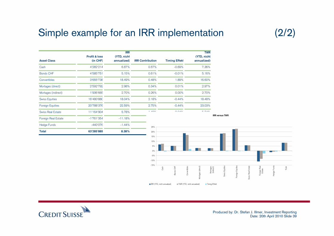
Asset ClassProfit & loss
(in CHF)
IRR(YTD, nicht
annualized) IRR Contribution Timing Effekt
TWR(YTD, nicht
annualized)
Cash 4'282'214 6.67% 0.57% -0.69% 7.36%
Bonds CHF 4'585'751 5.15% 0.61% -0.01% 5.16%
Convertibles 3'655'738 18.49% 0.48% 1.89% 16.60%
Mortages (direct) 2'592'792 2.98% 0.34% 0.01% 2.97%
Mortages (indirect) 1'936'665 2.70% 0.26% 0.00% 2.70%
Swiss Equities 16'480'880 18.04% 2.18% -0.44% 18.48%
Foreign Equities 20'788'376 22.59% 2.75% -0.44% 23.03%
Swiss Real Estate 11'164'904 5.78% 1.48% 0.04% 5.74%
Foreign Real Estate -1'761'354 -11.18% -0.23% -2.71% -8.47%
Hedge Funds -440'076 -1.44% -0.06% -0.68% -0.76%
Total 63'285'889 8.38% 8.38% 0.00% 8.38%
IRR versus TWR
-15%
-10%
-5%
0%
5%
10%
15%
20%
25%
Cas
h
Bon
ds C
HF
Con
vert
ible
s
Mor
tage
s (d
irect
)
Mor
tage
s(in
dire
ct)
Sw
iss
Equ
ities
Fore
ign
Equ
ities
Sw
iss
Rea
l Est
ate
Fore
ign
Rea
lE
stat
e
Hed
ge F
unds
Tota
l
IRR (YTD, nicht annualized) TWR (YTD, nicht annualized) Timing Effekt
Simple example for an IRR implementation (2/2)

Produced by: Dr. Stefan J. Illmer, Investment ReportingDate: 20th April 2010 Slide 40
Comments and Questions
Produced by: Dr. Stefan J. Illmer, Investment ReportingDate: 20th April 2010 Slide 41
References
Produced by: Dr. Stefan J. Illmer, Investment ReportingDate: 20th April 2010 Slide 42
References
“Determinants of Portfolio Performance”; in: Financial Analysts Journal; July 1986; by G. Brinson, R. Hood & G. Beebower
“Investment Performance Measurement”; by Bruce J. Feibel
“Decomposing the Money-Weighted Rate of Return”; in: Journal of Performance Measurement; Summer 2003; page 42-50; by Stefan J. Illmer and Wolfgang Marty
“Decomposing the Money-Weighted Rate of Return”; at the Performance Attribution Risk Management 11th Annual; 5th of November 2003; by Stefan J. Illmer
“Decomposing the Money-Weighted Rate of Return - an Update”; in: Journal of Performance Measurement; Fall 2009; page 22-29; by Stefan J. Illmer