1

Advanced Workshop on Structural Biology:

“Using Synchrotron Radiation to Visualise Biological Molecules” 15-19 December 2014

Diffraction Data Processing

with iMOSFLM, POINTLESS and SCALAMichele Cianci, EMBL, Hamburg

Authors

Harry Powell Geoff Batty Luke Kontogiannis Owen Johnson

CCP4, MRC

and BBSRC

for support Phil Evans Andrew Leslie

2

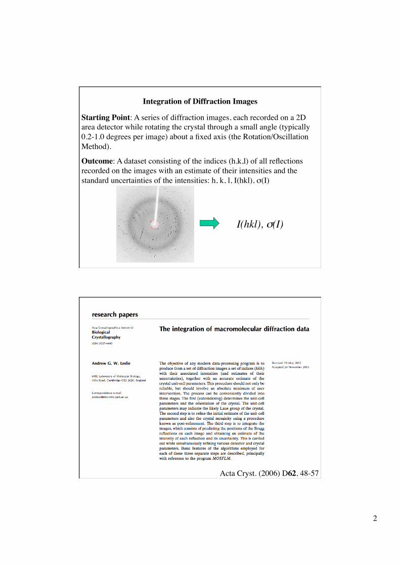
Starting Point: A series of diffraction images, each recorded on a 2D area detector while rotating the crystal through a small angle (typically 0.2-1.0 degrees per image) about a fixed axis (the Rotation/Oscillation Method).

Outcome: A dataset consisting of the indices (h,k,l) of all reflections recorded on the images with an estimate of their intensities and the standard uncertainties of the intensities: h, k, l, I(hkl), σ(I)

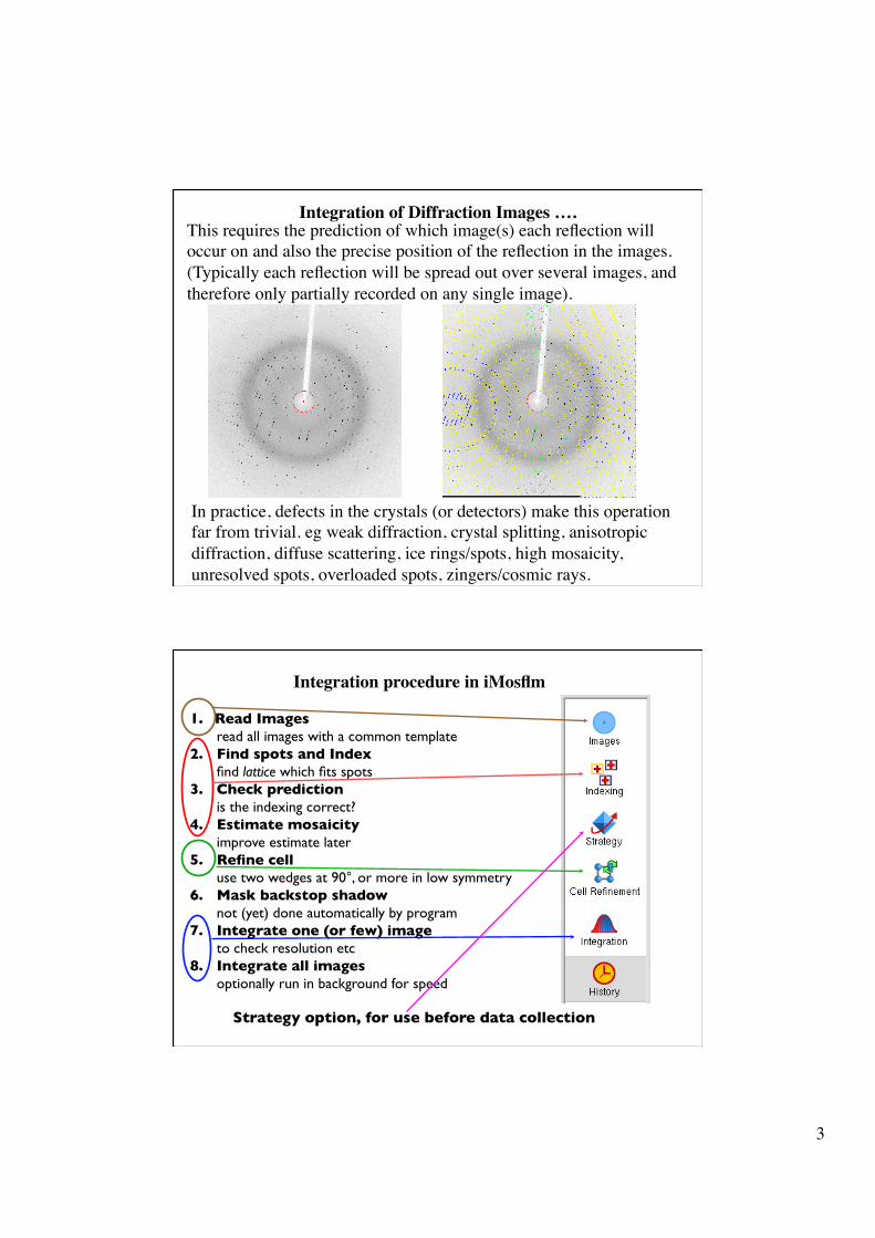
Integration of Diffraction Images

I(hkl), σ(I)

Acta Cryst. (2006) D62, 48-57

3

This requires the prediction of which image(s) each reflection will occur on and also the precise position of the reflection in the images. (Typically each reflection will be spread out over several images, and therefore only partially recorded on any single image).

In practice, defects in the crystals (or detectors) make this operation far from trivial. eg weak diffraction, crystal splitting, anisotropic diffraction, diffuse scattering, ice rings/spots, high mosaicity, unresolved spots, overloaded spots, zingers/cosmic rays.

Integration of Diffraction Images ….

Integration procedure in iMosflm

1.   Read Imagesread all images with a common template

2. Find spots and Indexfind lattice which fits spots

3. Check predictionis the indexing correct?

4. Estimate mosaicityimprove estimate later

5. Refine celluse two wedges at 90°, or more in low symmetry

6. Mask backstop shadownot (yet) done automatically by program

7. Integrate one (or few) imageto check resolution etc

8. Integrate all imagesoptionally run in background for speed

Strategy option, for use before data collection

4

AutoindexingObjective: To determine the unit cell, probable Laue group symmetry and orientation. (Note that intensities are required to find the true symmetry).

The spot positions in a diffraction image are a distorted projection of the reciprocal lattice. Using the Ewald sphere construction, the observed reflections (Xd, Yd, Φ) can be mapped back into reciprocal space giving a set of scattering vectors si.

r = sqrt( Xd2 + Yd

2 + D2)

D/r - 1

s = Xd/r

Yd/r

D is crystal to detector distance. Uncertainty in Φ leads to errors in s

Lattice: a Triclinic; m monoclinic; o orthorhombic; t tetragonal; h hexagonal; c cubic P primitive; C C-face centred; I body-centred; F face-centred; R rhombohedral

A “penalty” is associated with each solution, which reflects how well the determined cell obeys the constraints for that lattice type.

The solution with the highest symmetry from the group of solutions with low penalties (highlighted in blue) is usually chosen as the correct solution, but in cases of pseudosymmetry (eg monoclinic with β ~ 90o) the rms error in spot positions (σ(x,y)) is also important.

Auto-indexing procedures generate a list of possible solutions

5

An example of pseudo-symmetry

Based on the penalties, the lattice would be assigned as cubic, but the rms error in spot positions is 0.34mm for the cubic solution, but only 0.18mm for the (correct) orthorhombic solution.

Autoindexing….Refining the cell parameters

The cell obtained from the autoindexing is refined to get the best fit to the observed spot positions.

During this refinement, the cell parameters are forced to obey the restrictions imposed by the symmetry of the chosen solution

(eg α=β=γ=90 for an orthorhombic solution, a=b for trigonal, tetragonal, hexagonal).

The direct beam coordinates and optionally the detector distance are refined at the same time.

The rms error in spot positions after refinement can sometimes be used to distinguish between the real symmetry and higher pseudo-symmetry.

6

Autoindexing….Criteria for success

•  Having a sufficient number of spots (preferably a few hundred although 50 may be enough).

•  Correct wavelength, direct beam position, detector distance.

•  Only a single lattice present (2 lattices OK if one is weaker).

•  Reasonable mosaic spread (no overlap of adjacent lunes).

•  Resolved spots.

Absence of a clear separation between solutions with low penalties and solutions with high penalties can indicate errors in direct beam position, wavelength, distance etc (or a triclinic solution).

Results from a single image can be misleading for low symmetries.

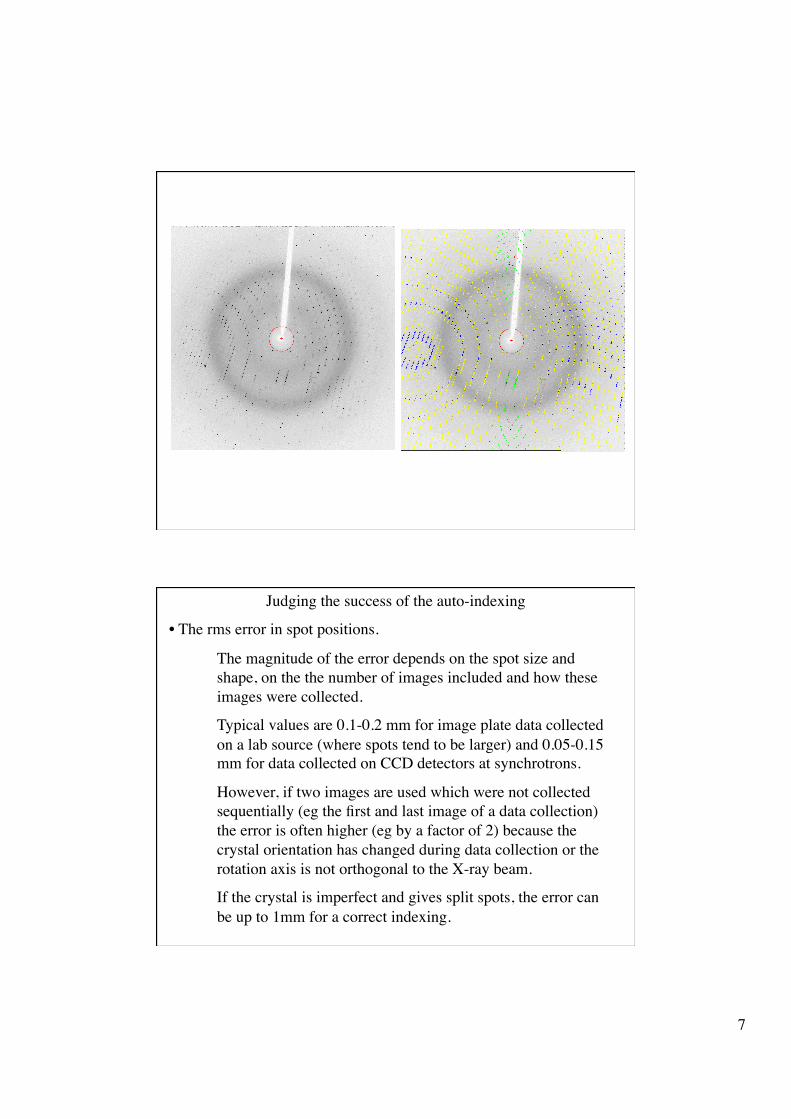
Judging the success of the auto-indexing

•  Does the predicted pattern match the image ?

Unless mosaic spread has been estimated, not all spots will be predicted. If two non-sequential images were used the prediction may be very slightly off.

Beware of under-predicting (if there is a systematic variation in the intensity of adjacent spots, eg every 2nd spot is weak).

Beware of over-predicting if a cell edge has been doubled (rare).

7

Judging the success of the auto-indexing

•  The rms error in spot positions.

The magnitude of the error depends on the spot size and shape, on the the number of images included and how these images were collected.

Typical values are 0.1-0.2 mm for image plate data collected on a lab source (where spots tend to be larger) and 0.05-0.15 mm for data collected on CCD detectors at synchrotrons.

However, if two images are used which were not collected sequentially (eg the first and last image of a data collection) the error is often higher (eg by a factor of 2) because the crystal orientation has changed during data collection or the rotation axis is not orthogonal to the X-ray beam.

If the crystal is imperfect and gives split spots, the error can be up to 1mm for a correct indexing.

8

Mosaicity Estimation

Predict pattern with increasing values for the mosaic spread (eg 0.0, 0.05, 0.1, 0.15 degrees). In each case, measure the total intensity of all predicted reflections. The mosaicity can be estimated from the plot of total intensity vs mosaic spread.

Parameter Refinement

Generally, once an orientation matrix and cell parameters have been derived from the autoindexing procedures described, these parameters are refined further using different algorithms.

Parameters to be refined:

1) Crystal parameters: Cell dimensions, orientation, mosaic spread.

2) Detector parameters: Detector position, orientation and (if appropriate) distortion

parameters.

3) Beam parameters: Orientation, beam divergence.

9

Two types of refinement

1) Using spot coordinates and a positional residual:

Ω1 = Σi ωix(Xicalc- Xi

obs)2 + ωiy(Yicalc- Yi

obs)2

2) Using spot position in Φ and an angular residual:

Ω2 = Σi ωi[(Ricalc- Ri

obs)/di* ]2

where Ricalc,Ri

obs are the calculated and observed distances of the reciprocal lattice point di

* from the centre of the Ewald sphere (Post refinement).

The positional residual gives no information about small errors in the crystal orientation around the spindle axis, or about the mosaic spread.The angular residual gives no information on the detector parameters (because it does not depend on spot positions).

Refinement based on spot coordinates

The refined parameters are:

i) The crystal to detector distance.

ii) The position of the centre of the diffraction pattern.

iii) A relative scale factor applied to the Y coordinates, YSCALE (allows for errors in cell parameters, or different pixel sizes in X and Y) .

iv) Small rotations of the detector about a horizontal axis and a vertical axis (TILT and TWIST).

v) Rotation of the detector about the X-ray beam direction.

vi) Radial (ROFF) and tangential offsets (TOFF) for images plates with spiral readout.

10

Why refine parameters that should not change ?

Parameters such as the detector distance and YSCALE would not be expected to change during an experiment (although small changes in distance can arise if the crystal is not centred on the rotation axis).

However, refining these parameters can compensate for errors in the cell parameters, and, in cases of significant radiation damage, for genuine variation in the cell during data collection.

During integration, the main objective is to get the best possible prediction of the spot positions.

A smoothly changing decrease in the refined detector distance can be an indicator of an increase in cell size due to radiation damage.

For weak images, parameters like the detector twist and tilt are not well defined, and if they show a lot of variation should be fixed at the mean value.

Determining accurate cell parameters using Post Refinement

Post-refinement uses the distribution of the intensity of partially recorded reflections over adjacent images, together with a model for the “rocking curve”, to determine the exact phi value at which a reciprocal lattice point lies exactly on the Ewald sphere. Note that at least two images are required.

11

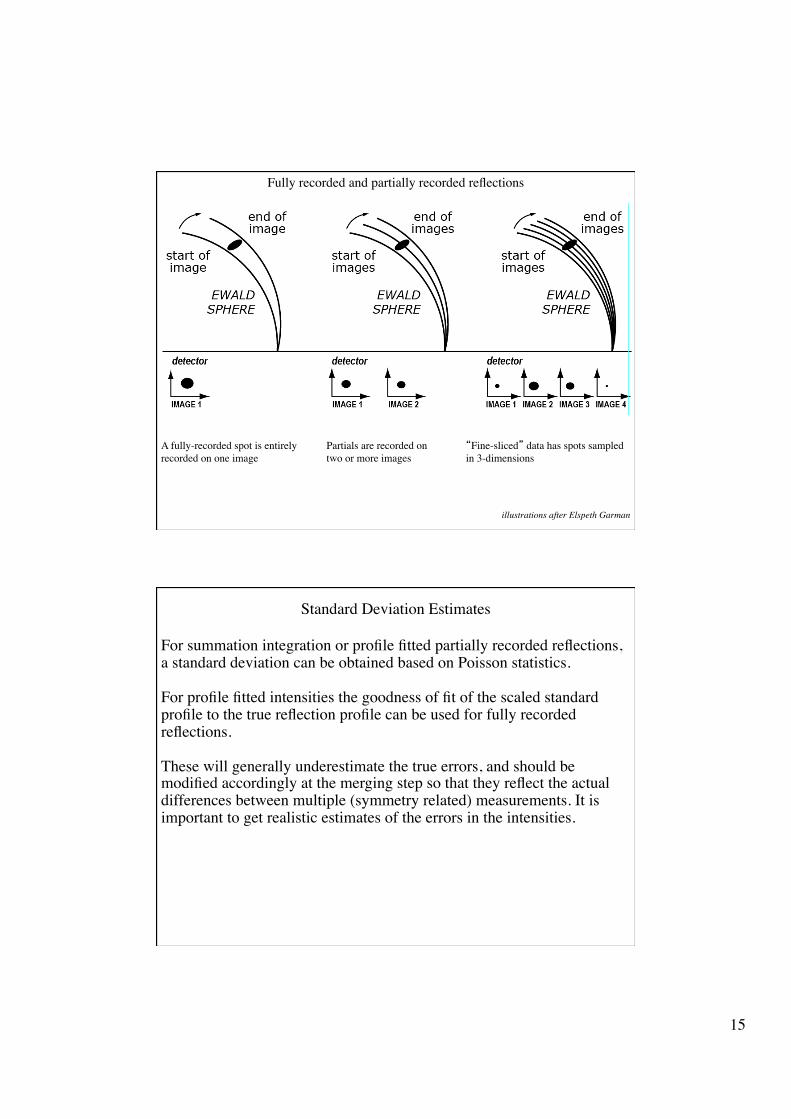
A fully-recorded spot is entirely recorded on one image

Partials are recorded on two or more images

“Fine-sliced” data has spots sampled in 3-dimensions

illustrations after Elspeth Garman

Fully recorded and partially recorded reflections

The radius of a reciprocal lattice point (ε) is modelled by:

Consider a partially recorded reflection spread over two images, with a recorded intensity I1 on the first and I2 on the second. To determine the “observed” position, Pʹ′ from the fraction of the total intensity that is observed on the first image , F = I1/(I1+I2), requires a model for the “rocking curve”, eg:

Knowing F and ε, ΔR, the distance of Pʹ′ from the sphere, can be calculated, giving Robs. (The plus or minus sign depends on whether the rlp is entering or exiting the sphere).

Post Refinement

Refine cell, orientation and mosaicity to minimise the angular residual (δ):

12

Post Refinement Provides Very Accurate Cell Parameters

Using a few degrees of data in two segments widely separated in phi will typically give cell parameters that are accurate to a few parts in 10,000 (for resolutions higher than ~2.8Å). Two segments are essential for orthorhombic or lower symmetry, three or four are recommended for triclinic.

The crystal orientation is determined to better than 0.01 degrees (for crystals with typical mosaicity, less accurately for high mosaicity).

Ideally, the cell should be refined by post refinement prior to integration of the images, and fixed during the integration.

Integration of the Images

Step 1: Predict the position in the digitised image of each Bragg reflection.

Step 2: Estimate its intensity (need to subtract the X-ray background) and an error estimate of the intensity.

1)  Predicting reflection positions

Accuracy in prediction is crucial. Ideally, cell parameters should be known to better than 0.1%. Errors in prediction will introduce systematic errors in profile fitting.

Typically the detector parameters, crystal orientation and mosaic spread will be refined for every image during the integration. The cell parameters are not normally refined.

13

2) Determining the X-ray backgroundThe background can only be measured in a region around the spot either in two dimensions (X, Y, the detector co-ordinates) for coarse phi-slices or in 3 dimensions (X, Y and phi) for fine phi slices.

Requires definition of a peak/background mask. A plane is fitted to pixels in the background region (rejecting any outliers), and the equation of this background plane is used to calculate the background for pixels in the peak region.

Errors in the mask definition will give systematic errors in intensities.

Summation integration and Profile FittingSummation integration:Sum the pixel values of all pixels in the peak area of the mask, and then subtract the sum of the background values calculated from the background plane for the same pixels.

Profile fitting:Assume that the shape or profile (in 2 or 3 dimensions) of the spots is known. Then determine the scale factor which, when applied to the known spot profile, gives the best fit to be observed spot profile. This scale factor is then proportional to the profile fitted intensity for the reflection. Minimise: R = Σ ωi (Xi - KPi)2

Xi is the background subtracted intensity at pixel iPi is the value of the standard profile at the corresponding pixelωi is a weight, derived from the expected variance of XiK is the scale factor to be determined

14

Determining the "Standard" ProfileThe profiles are determined empirically (as the average of many spots). The spot shape varies according to position on the detector, and this must be allowed for (different programs do this in different ways).

Need to take precautions to avoid introducing systematic errors due to broadening profiles during averaging.For each reflection integrated, a new profile is calculated as a weighted mean of the “standard” profiles for the adjacent regions.Profile fitting is used for both fully recorded and partially recorded reflections. Although this is strictly not valid, in practice it works well.

The advantages of profile fitting

Profile fitting provides a more reliable estimate of the spot intensity for weak reflections than summation integration. It can be shown that the effect of profile fitting is to effectively “down-weight” the peripheral peak pixels (where the signal to noise is lowest) relative to the central pixels (where the signal to noise is highest).(See AGW Leslie, Acta Cryst D55, 1696-1702,1999)

15

A fully-recorded spot is entirely recorded on one image

Partials are recorded on two or more images

“Fine-sliced” data has spots sampled in 3-dimensions

illustrations after Elspeth Garman

Fully recorded and partially recorded reflections

Standard Deviation Estimates

For summation integration or profile fitted partially recorded reflections, a standard deviation can be obtained based on Poisson statistics.

For profile fitted intensities the goodness of fit of the scaled standard profile to the true reflection profile can be used for fully recorded reflections.

These will generally underestimate the true errors, and should be modified accordingly at the merging step so that they reflect the actual differences between multiple (symmetry related) measurements. It is important to get realistic estimates of the errors in the intensities.

16

Scaling slides from Phil Evans

Acta Cryst. (2006) D62, 72 -82

Protocol for space group determination (program POINTLESS by Phil Evans)

Pointless reads the MTZ file output by MOSFLM (ie before any scaling or averaging). It can be run on a (very) incomplete dataset.

1.  From the unit cell dimensions, find the highest compatible lattice symmetry (within a tolerance). This may be higher than the symmtery used when integrating the data. The input symmetry is ignored.

2. Score each symmetry element (rotation) belonging to lattice symmetry using all pairs of observations related by that element.

3. Score combinations of symmetry elements for all possible sub-groups (Laue groups) of lattice symmetry group.

4. Score possible space groups from axial systematic absences.

Scoring functions for rotational symmetry based on correlation coefficient, since this relatively independent of the unknown scales. Rmeas values are also calculated

17

Only the orthorhombic symmetry operators are present

Correlation coefficient on E2 Rfactor (multiplicity weighted)

Nelmt Lklhd Z-cc CC N Rmeas Symmetry & operator (in Lattice Cell)

1 0.808 5.94 0.89 9313 0.115 identity 2 0.828 6.05 0.91 14088 0.141 *** 2-fold l ( 0 0 1) {-h,-k,+l} 3 0.000 0.06 0.01 16864 0.527 2-fold ( 1-1 0) {-k,-h,-l} 4 0.871 6.33 0.95 10418 0.100 *** 2-fold ( 2-1 0) {+h,-h-k,-l} 5 0.000 0.53 0.08 12639 0.559 2-fold h ( 1 0 0) {+h+k,-k,-l} 6 0.000 0.06 0.01 16015 0.562 2-fold ( 1 1 0) {+k,+h,-l} 7 0.870 6.32 0.95 2187 0.087 *** 2-fold k ( 0 1 0) {-h,+h+k,-l} 8 0.000 0.55 0.08 7552 0.540 2-fold (-1 2 0) {-h-k,+k,-l} 9 0.000 -0.12 -0.02 11978 0.598 3-fold l ( 0 0 1) {-h-k,+h,+l} {+k,-h-k,+l} 10 0.000 -0.06 -0.01 17036 0.582 6-fold l ( 0 0 1) {-k,+h+k,+l} {+h+k,-h,+l}

Z-score(CC)“Likelihood”

Example: a C222 cell that is pseudo hexagonal

Score each symmetry operator in P622

A clear preference for Laue group Cmmm

Net Z(CC) Likelihood

Correlation coefficient & R-factor

Cell deviation

Net Z(CC) scores are Z+(symmetry in group) - Z-(symmetry not in group)

Likelihood allows for the possibility of pseudo-symmetry

Laue Group Lklhd NetZc Zc+ Zc- CC CC- Rmeas R- Delta ReindexOperator > 1 C m m m *** 0.991 6.00 6.12 0.12 0.93 0.02 0.12 0.56 0.1 [1/2h1/2k,3/2h+1/2k,l] > 2 C 1 2/m 1 0.367 5.00 6.13 1.13 0.95 0.17 0.10 0.48 0.1 [3/2h+1/2k,-1/2h+1/2k,l] > 3 C 1 2/m 1 0.365 4.55 6.04 1.49 0.95 0.22 0.09 0.46 0.1 [1/2h-1/2k,3/2h+1/2k,l] > 4 P 1 2/m 1 0.250 4.88 5.99 1.11 0.91 0.17 0.14 0.49 0.0 [1/2h+1/2k,l,1/2h-1/2k] 5 P -1 0.031 4.27 5.94 1.67 0.89 0.25 0.12 0.44 0.0 [-1/2h+1/2k,-1/2h-1/2k,l] 6 C 1 2/m 1 0.000 2.45 4.18 1.73 0.08 0.26 0.54 0.44 0.1 [3/2h-1/2k,1/2h+1/2k,l] 7 C 1 2/m 1 0.000 1.62 3.40 1.79 0.08 0.27 0.56 0.43 0.1 [-1/2h-1/2k,3/2h-1/2k,l] 8 C 1 2/m 1 0.000 0.60 2.55 1.95 0.01 0.29 0.56 0.42 0.0 [-k,h,l] 9 C 1 2/m 1 0.000 0.57 2.52 1.96 0.01 0.29 0.53 0.43 0.0 [h,k,l] 10 P -3 0.000 0.75 2.68 1.93 -0.02 0.29 0.60 0.42 0.1 [1/2h-1/2k,1/2h+1/2k,l] 11 C m m m 0.000 2.60 3.80 1.20 0.44 0.18 0.38 0.47 0.1 [-1/2h-1/2k,3/2h-1/2k,l] =12 C m m m 0.000 0.94 2.59 1.65 0.26 0.25 0.42 0.46 0.0 [h,k,l] 13 P 6/m 0.000 0.83 2.54 1.70 0.24 0.26 0.45 0.44 0.1 [1/2h-1/2k,1/2h+1/2k,l] 14 P -3 m 1 0.000 0.72 2.46 1.74 0.24 0.26 0.45 0.44 0.1 [1/2h-1/2k,1/2h+1/2k,l] 15 P -3 1 m 0.000 -0.57 1.79 2.36 0.10 0.35 0.52 0.39 0.1 [1/2h-1/2k,1/2h+1/2k,l] 16 P 6/m m m 0.000 2.09 2.09 0.00 0.25 0.00 0.44 0.00 0.1 [1/2h-1/2k,1/2h+1/2k,l]

Reindexing

18

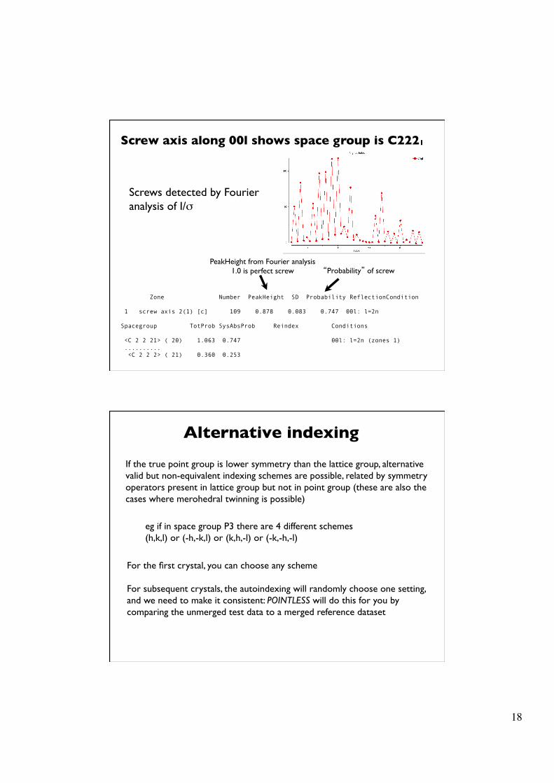
Zone Number PeakHeight SD Probability ReflectionCondition 1 screw axis 2(1) [c] 109 0.878 0.083 0.747 00l: l=2n Spacegroup TotProb SysAbsProb Reindex Conditions <C 2 2 21> ( 20) 1.063 0.747 00l: l=2n (zones 1) .......... <C 2 2 2> ( 21) 0.360 0.253

Screw axis along 00l shows space group is C2221

PeakHeight from Fourier analysis1.0 is perfect screw “Probability” of screw

Screws detected by Fourier analysis of I/σ

Alternative indexing

If the true point group is lower symmetry than the lattice group, alternative valid but non-equivalent indexing schemes are possible, related by symmetry operators present in lattice group but not in point group (these are also the cases where merohedral twinning is possible)

eg if in space group P3 there are 4 different schemes ���(h,k,l) or (-h,-k,l) or (k,h,-l) or (-k,-h,-l)

For the first crystal, you can choose any scheme

For subsequent crystals, the autoindexing will randomly choose one setting, and we need to make it consistent: POINTLESS will do this for you by comparing the unmerged test data to a merged reference dataset

19

Data Processing: ScalingThe scaling and merging step is important because

•  it attempts to put all observations on a common scale•  it provides the main diagnostics of data quality and whether the data collection is satisfactory

Because of this diagnostic role, it is important that data are scaled as soon as possible after collection, or during collection, preferably while the crystal is still on the camera.

Why are reflections on different scales?

Various physical factors lead to observed intensities being on different scales. Scaling models should if possible parameterise the experiment so different experiments may require different models

Understanding the effect of these factors allows a sensible design of correction and an understanding of what can go wrong

1) Factors related to incident beam and the rotation camera2) Factors related to the crystal and the diffracted beam3) Factors related to the detector

20

1) Factors related to incident Xray beam•  Incident beam intensity: variable on synchrotrons and not normally measured. Assumed to be constant during a single image, or at least varying smoothly and slowly (relative to exposure time). If this is not true, the data will be poor.

•  Illuminated volume: changes with φ if beam smaller than crystal.

•  Absorption in primary beam by crystal: indistinguishable from illuminated volume changes.

•  Variations in rotation speed and shutter synchronisation: These errors are disastrous, difficult to detect, and impossible to correct for: we assume that the crystal rotation rate is constant and that adjacent images exactly abut in φ. Shutter synchronisation errors lead to partial bias which may be positive, unlike the usual negative bias.

2) Factors related to crystal and diffracted beam

•  Absorption in secondary beam - serious at long wavelength (including CuKα), worth correcting for SAD/MAD data, especially sulphur SAD.

•  Radiation damage - serious on high brilliance sources. Not correctable unless small as the structure is changing. Extrapolation to zero (quarter) dose successful in some cases (Kay Diederich).

The relative B-factor is largely a correction for radiation damage

21

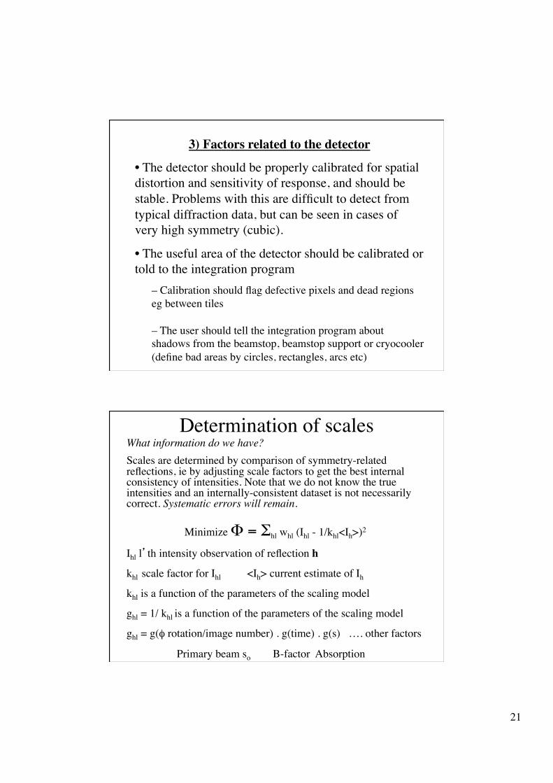
3) Factors related to the detector

• The detector should be properly calibrated for spatial distortion and sensitivity of response, and should be stable. Problems with this are difficult to detect from typical diffraction data, but can be seen in cases of very high symmetry (cubic).

• The useful area of the detector should be calibrated or told to the integration program

– Calibration should flag defective pixels and dead regions eg between tiles

– The user should tell the integration program about shadows from the beamstop, beamstop support or cryocooler (define bad areas by circles, rectangles, arcs etc)

Determination of scalesWhat information do we have?Scales are determined by comparison of symmetry-related reflections, ie by adjusting scale factors to get the best internal consistency of intensities. Note that we do not know the true intensities and an internally-consistent dataset is not necessarily correct. Systematic errors will remain.

Minimize Φ = Σhl whl (Ihl - 1/khl<Ih>)2

Ihl l’th intensity observation of reflection h

khl scale factor for Ihl <Ih> current estimate of Ih

khl is a function of the parameters of the scaling model

ghl = 1/ khl is a function of the parameters of the scaling model

ghl = g(φ rotation/image number) . g(time) . g(s) …. other factors

Primary beam so B-factor Absorption

22

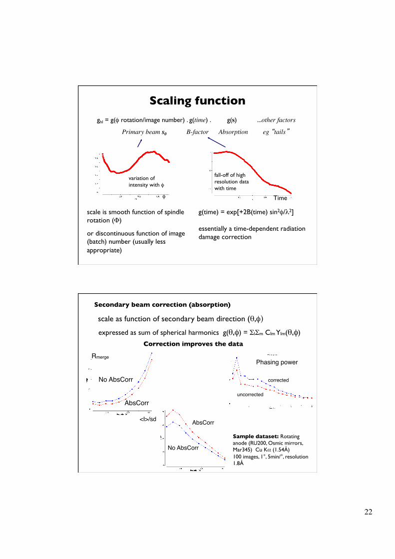
ghl = g(φ rotation/image number) . g(time) . g(s) ...other factors

Primary beam s0 B-factor Absorption eg “tails”

Scaling function

scale is smooth function of spindle rotation (Φ)

or discontinuous function of image (batch) number (usually less appropriate)

g(time) = exp[+2B(time) sin2φ/λ2]

essentially a time-dependent radiation damage correction

Time

fall-off of high resolution data with time

variation of intensity with φ

φ

Sample dataset: Rotating anode (RU200, Osmic mirrors, Mar345) Cu Kα (1.54Å)100 images, 1°, 5min/°, resolution 1.8Å

Rmerge

No AbsCorr

AbsCorr

No AbsCorr

AbsCorr<I>/sd

Correction improves the data

corrected

uncorrected

Phasing power

expressed as sum of spherical harmonics g(θ,φ) = ΣlΣm Clm Ylm(θ,φ)

Secondary beam correction (absorption)

scale as function of secondary beam direction (θ,φ)

23

What to look at ?How well do equivalent observations agree with each other ?

1. R-factors

(a) Rmerge (Rsym) = Σ | Ihl - <Ih> | / Σ | <Ih> |

This is the traditional measure of agreement, but it increases with higher multiplicity even though the merged data is

better.

(b) Rmeas = Rr.i.m.= Σ √(n/n-1) | Ihl - <Ih> | / Σ | <Ih> |

The multiplicity-weight R-factor allows for the improvement in data with higher multiplicity. This is particularly useful when comparing different possible point-groups.

Diederichs & Karplus, Nature Structural Biology, 4, 269-275 (1997)Weiss & Hilgenfeld, J.Appl.Cryst. 30, 203-205 (1997)

2. Intensities and standard deviations: what is the real resolution ?

(a) Corrected σ’(Ihl)2 = SDfac2 [σ2 + SdB <Ih> + (SdAdd <Ih>)2]

The corrected σ’(I) is compared with the intensities: the most useful statistic is < <I>/ σ (<I>) > (labelled Mn(I)/sd in table) as a function of resolution

This statistic shows the improvement of the estimate of <I> with multiple measurements. It is the best indicator of the true resolution limit

< <I>/ σ(<I>) > greater than ~ 2 (or so)

Maybe lower for anisotropic data, 1.5 to 1.0

(b) Correlation between half datasets (random halves)

ResolutionCor

rela

tion

coef

ficie

nt

Correlation of <I> indicating a resolution limit

24

Are some parts of the data bad ?

Analysis of Rmerge against batch number gives a very clear indication of problems local to some regions of the data. Perhaps something has gone wrong with the integration step, or there are some bad images

Here the beginning of the dataset is wrong due to problems in integration

Do the parameters (k, B etc) make physical sense ?

These scale factors follow a reasonable absorption curve

These B-factors are not sensibleAs well as being highly variable, they are also positive: Bfactors should be negative (ie sharpening later observations)

25

Partial biasThis measures the systematic difference between fulls and summed partials (if there are any fully recorded observations).

Fractional Bias = Σ (<Ifull> - Ipartial) / Σ <I>

Typically, its value is negative, ie the summed partials are bigger than the fulls, due to truncation of diffuse scattering tails on fulls (a partially-recorded observation is recorded over at least twice the angular range of a full)

Negative bias may be corrected (very approximately) by the TAILS correction

A positive bias generally indicates some serious problem with the data collection (shutter mistiming, rotation speed variation)

OutliersDetection of outliers is easiest if the multiplicity is high

Removal of spots behind the backstop shadow does not work well at present: usually it rejects all the good ones, so tell Mosflm where the backstop shadow is

Scala also has facilities for omitting regions of the detector (rectangles and arcs of circles)

Inspect the ROGUES file to see what is being rejected (at least occasionally)

The ROGUES file contains all rejected reflections (flag "*", "@" for I+- rejects, "#" for Emax rejects) TotFrc = total fraction, fulls (f) or partials (p) Flag I+ or I- for Bijvoet classes DelI/sd = (Ihl - Mn(I)others)/sqrt[sd(Ihl)**2 + sd(Mn(I))**2] h k l h k l Batch I sigI E TotFrc Flag Scale LP DelI/sd d(A) Xdet Ydet Phi (measured) (unique) -2 -2 0 2 2 0 1220 24941 2756 1.03 0.95p I- 2.434 0.031 -1.1 30.40 1263.7 1103.2 210.8 -4 2 0 2 2 0 1146 9400 2101 0.63 0.99p *I+ 3.017 0.032 -6.7 30.40 1266.4 1123.3 151.3 4 -2 0 2 2 0 1148 27521 2972 1.08 1.09p I- 2.882 0.032 0.0 30.40 1058.8 1130.0 153.2 2 -4 0 2 2 0 1075 29967 2865 1.13 0.92p I+ 2.706 0.032 1.1 30.40 1060.9 1106.6 94.4 Weighted mean 27407

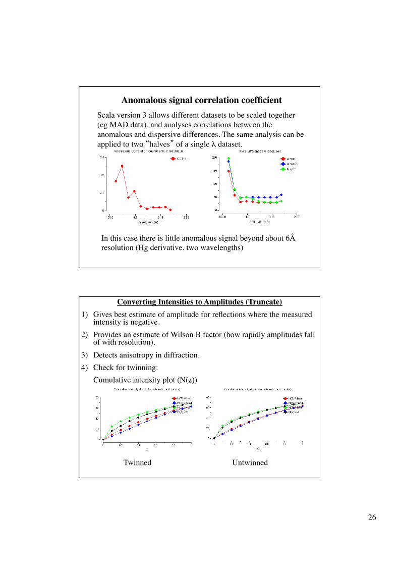
26

Anomalous signal correlation coefficientScala version 3 allows different datasets to be scaled together (eg MAD data), and analyses correlations between the anomalous and dispersive differences. The same analysis can be applied to two “halves” of a single λ dataset.

In this case there is little anomalous signal beyond about 6Å resolution (Hg derivative, two wavelengths)

Converting Intensities to Amplitudes (Truncate)1)  Gives best estimate of amplitude for reflections where the measured

intensity is negative.2)  Provides an estimate of Wilson B factor (how rapidly amplitudes fall

of with resolution).3)  Detects anisotropy in diffraction.4)  Check for twinning:

Cumulative intensity plot (N(z))

Twinned Untwinned