DATA MINING 2Advanced ClusteringRiccardo Guidotti

a.a. 2020/2021

K-Means Extensions

Bisecting K-Means

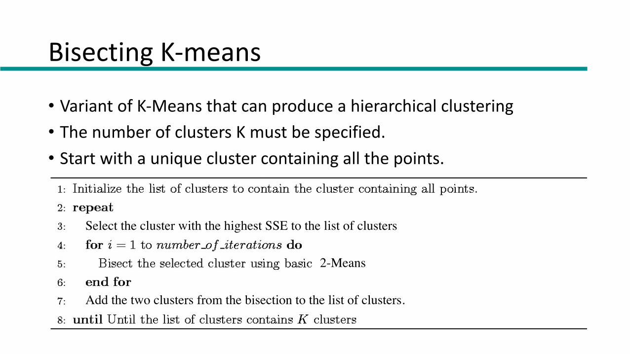
Bisecting K-means

• Variant of K-Means that can produce a hierarchical clustering• The number of clusters K must be specified.• Start with a unique cluster containing all the points.

2-Means

Select the cluster with the highest SSE to the list of clusters

Add the two clusters from the bisection to the list of clusters.

Bisecting K-means Limitations

• The algorithm can be also exhaustive and terminating at a singleton clusters if K is not specified.• Terminating at singleton clusters • Is time consuming• Singleton clusters are meaningless (i.e., over-splitting)• Intermediate clusters are more likely to correspond to real classes

• Bisecting K-Means do not uses any criterion for stopping bisections before singleton clusters are reached.

K-Means Extensions

X-Means

Bayesian Information Criterion (BIC)

• A strategy to stop the Bisecting algorithm when meaningful clusters are reached to avoid over-splitting.• The BIC can be adopted as splitting

criterion of a cluster in order to decide whether a cluster should split or no.• BIC measures the improvement of the

cluster structure between a cluster and its two children clusters.• If the BIC of the parent is less than BIC of

the children than we accept the bisection.

Two resultingclusters:BIC(K=2)=2245

1C Parent cluster:BIC(K=1)=1980

1C 2C

C

X-Means

For k in a given range [r1,rmax]: 1. Improve Params: run K-Means with with the current k.2. Improve Structure: recursively split each cluster in two (Bisecting 2-

Means) and use local BIC to decide to keep the split. Stop if the current structure does not respect local BIC or the number of clusters is higher than rmax.

3. Store the actual configuration with a global BIC calculated on the whole configuration

4. If k > rmax stop and return the best model w.r.t. the global BIC.

X-Means1. K-means with k=3

2. Split each centroid in 2 children moved a distance proportional to the region size in opposite direction (random)

3. Run 2-means in each region locally 4. Compare BIC of parent

and children4. Only centroids with higher BIC survives

BIC Formula in X-Means

• The BIC score of a data collection is defined as (Kass and Wasserman, 1995):

• is the log-likelihood of the dataset D

• pj is a function of the number of independent parameters: centroids coordinates, variance estimation.

• R is the number of points of a cluster, M is the number of dimensions

• Approximate the probability that the clustering in Mj is describing the real clusters in the data

BIC(Mj)= l

jD⎛⎝⎜

⎞⎠⎟−pj

2logR

( )jl D

BIC Formula in X-Means

• Adjusted Log-likelihood of the model.• The likelihood that the data is “explained by” the clusters according to the

spherical-Gaussian assumption of K-Means

• Focusing on the set Dn of points which belong to centroid n

• It estimates how closely to the centroid are the points of the cluster.

BIC(Mj)= l

jD⎛⎝⎜

⎞⎠⎟−pj

2logR

K-Means Origins

Expectation Maximization

Model-based Clustering (probabilistic)

• In order to understand our data, we will assume that there is a generative process (a model) that creates/describes the data, and we will try to find the model that best fits the data.• Models of different complexity can be defined, but we will assume that our

model is a distribution from which data points are sampled• Example: the data is the height of all people in Greece

• In most cases, a single distribution is not good enough to describe all data points: different parts of the data follow a different distribution• Example: the data is the height of all people in Greece and China• We need a mixture model• Different distributions correspond to different clusters in the data.

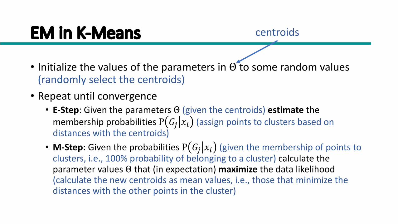
Expectation Maximization Algorithm

• Initialize the values of the parameters in Θ to some random values• Repeat until convergence• E-Step: Given the parameters Θ estimate the membership probabilities P 𝐺! 𝑥"• M-Step: Given the probabilities P 𝐺! 𝑥" , calculate the parameter values Θ that

(in expectation) maximize the data likelihood

• Examples• E-Step: Assignment of points to clusters

• K-Means: hard assignment, EM: soft assignment• M-Step: Parameters estimation

• K-Means: Computation of centroids, EM: Computation of the new model parameters

EM in K-Means

• Initialize the values of the parameters in Θ to some random values (randomly select the centroids) • Repeat until convergence• E-Step: Given the parameters Θ (given the centroids) estimate the

membership probabilities P 𝐺! 𝑥" (assign points to clusters based on distances with the centroids)• M-Step: Given the probabilities P 𝐺! 𝑥" (given the membership of points to

clusters, i.e., 100% probability of belonging to a cluster) calculate the parameter values Θ that (in expectation) maximize the data likelihood (calculate the new centroids as mean values, i.e., those that minimize the distances with the other points in the cluster)

centroids

Expectation Maximization Algorithm

K-Means Brother

Mixture Gaussian Model

Gaussian Distribution

• Example: the data is the height of all people in Greece• Experience has shown that this data follows a

Gaussian (Normal) distribution

Mixture Gaussian Model

• What is a model?• A Gaussian distribution is defined by the mean 𝜇 and the standard deviation 𝜎• We define our model as the pair of parameters 𝜃 = (𝜇, 𝜎)

• More generally, a model is defined as a vector of parameters 𝜃

• We want to find the normal distribution 𝑁(𝜇, 𝜎) that best fits our data• Find the best values for 𝜇 and 𝜎• But what does “best fit” mean?

Maximum Likelihood Estimation (MLE)• Suppose that we have a vector 𝑋 = {𝑥!, … , 𝑥"} of values• We want to fit a Gaussian model 𝑁(𝜇, 𝜎) to the data • Probability of observing a point 𝑥#

• Probability of observing all points (we assume independence)

• We want to find the parameters 𝜃 = (𝜇, 𝜎) that maximizes the probability 𝑃 𝑋 𝜃

Maximum Likelihood Estimation (MLE)

• The probability 𝑃 𝑋 𝜃 as a function of 𝜃 is the Likelihood function

• It is usually easier to work with the Log-Likelihood function

• Thus, the Maximum Likelihood Estimation for the Gaussian Model consists in finding the parameters 𝜇, 𝜎 that maximize 𝐿𝐿(𝜃)

Maximum Likelihood Estimation (MLE)

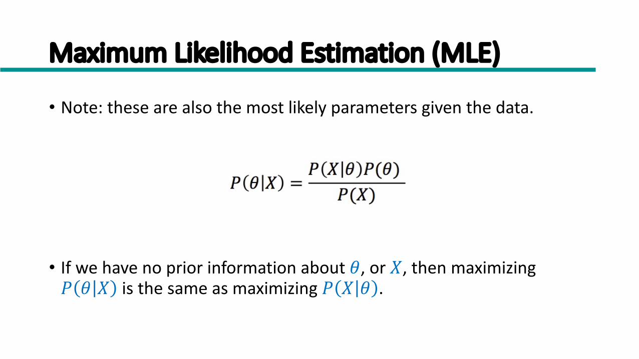
• Note: these are also the most likely parameters given the data.

• If we have no prior information about 𝜃, or 𝑋, then maximizing 𝑃 𝜃 𝑋 is the same as maximizing 𝑃 𝑋 𝜃 .

Mixture of Gaussians

• Suppose that you have the heights of people from Greece and China and the distribution looks like the figure below (dramatization)

Mixture of Gaussians

• In this case the data is the result of the mixture of two Gaussians • One for Greek people, and one for Chinese people• Identifying for each value which Gaussian is most likely to have generated it

will give us a clustering.

Mixture Model

• A value 𝑥# is generated according to the following process:• First select the nationality• With probability 𝜋#select Greek, with

probability 𝜋$ select China (𝜋# + 𝜋$ = 1)

• Given the nationality, generate the point from the corresponding Gaussian• 𝑃 𝑥" 𝜃# ~𝑁(𝜇# , 𝜎#) if Greece• 𝑃 𝑥" 𝜃$ ~𝑁(𝜇$ , 𝜎$) if China

Mixture Model

• Our model has the following parameters

• For value 𝑥!, we have:

• For all values 𝑋 = {𝑥%, … , 𝑥&}

• We want to estimate the parameters that maximize the Likelihood

Assign a point to a cluster. In K-Means they are the membership: hard assignment.

Describe a cluster. In K-Means they are the centroids.

Mixture Model

• Once we have the parameters 𝜃 = (𝜋$ , 𝜋% , 𝜇$ , 𝜎$ , 𝜇% , 𝜎%), we can estimate the membership probabilities 𝑃(𝐺|𝑥#) and 𝑃(𝐶|𝑥#) for each point 𝑥#:

• This is the probability that point 𝑥# belongs to the Greek or the Chinese population (cluster)

Mixture of Gaussians as EM

• Initialize the values of the parameters in 𝜃 to some random values• Repeat until convergence• E-Step: Given the parameters Θ estimate the membership probabilities P 𝐺 𝑥" and P 𝐶 𝑥" .• M-Step: Calculate the parameter values Θ that (in expectation) maximize the

data likelihood.

DBSCAN Evolution

OPTICS

When DBSCAN Works Well

Original Points Clusters

• Resistant to Noise

• Can handle clusters of different shapes and sizes

When DBSCAN Does NOT Work Well

Original Points

(MinPts=4, Eps=9.75).

(MinPts=4, Eps=9.92)

• Varying densities

• High-dimensional data

OPTICS

• OPTICS: Ordering Points To Identify the Clustering Structure• Produces a special order of the dataset wrt its density-based

clustering structure. • This cluster-ordering contains info equivalent to the density-based

clusterings corresponding to a broad range of parameter settings.• Good for both automatic and interactive cluster analysis, including

finding intrinsic clustering structure.• Can be represented graphically or using visualization techniques.

OPTICS: Extension from DBSCAN

• OPTICS requires two parameters: • ε, which describes the maximum distance

(radius) to consider,• MinPts, describing the number of points

required to form a cluster• Core point. A point p is a core point if at least

MinPts points are found within its ε-neighborhood.

• Core Distance. It is the minimum value of radius required to classify a given point as a core point. If the given point is not a Core point, then it’s Core Distance is undefined.

OPTICS: Extension from DBSCAN

• Reachability Distance. The reachability distance between a point p and q is the maximum of the Core Distance of p and the Distance between p and q.

• The Reachability Distance is not defined if qis not a Core point. Below is the example of the Reachability Distance.

• In other words, if q is within the core distance of p then use the core distance, otherwise the real distance.

OPTICS Pseudo-Code

• For each point p in the dataset• Initialize the reachability distance of p as undefined

• For each unprocessed point p in the dataset• Get the neighbors N of p• Mark p as processed and output to the ordered list• If p is a core point

• Initialize a priority queue Q to get the closest point to p in terms of reachability• Call the function update(N, p, Q)• For each point q in Q

• Get the neighbors N’ of q• Mark q as processed and output to the ordered list

• If q is a core point Call the function update(N’, q, Q)

OPTICS Pseudo-Code

• Function update(N, p Q)• Calculate the core distance for p• For each neighbor q in N (update the reachability)• If q is not processed• new_rd = reachability distance between p and q

• If q is not in Q• Q.insert(q, new_rd)

• Else• If new_rd < q.rd• Q.move_up(q, new_rd)

OPTICS Output

• OPTICS outputs the points in a particular ordering, annotated with their smallest reachability distance.• A reachability-plot (a special kind of dendrogram), the hierarchical

structure of the clusters can be obtained easily. • x-axis: the ordering of the points as processed by OPTICS • y-axis: the reachability distance • Points belonging to a cluster have a low reachability distance to their

nearest neighbor, the clusters show up as valleys in the reachability plot. The deeper the valley, the denser the cluster.

OPTICS Output

OPTICS Output

• Clusters are extracted 1. by selecting a range on the x-axis after visual inspection, 2. by selecting a threshold on the y-axis3. by different algorithms that try to detect the valleys by steepness, knee

detection, or local maxima. Clustering obtained this way usually are hierarchical, and cannot be achieved by a single DBSCAN run.

https://scikit-learn.org/stable/auto_examples/cluster/plot_optics.html#sphx-glr-auto-examples-cluster-plot-optics-py

e

e

Reachability-distance

Cluster-orderof the objects

undefined

e‘

OPTICS: The Radius Parameter

• Both core-distance and reachability-distance are undefined if no sufficiently dense cluster (w.r.t. ε) is available. • Given a sufficiently large ε, this never happens, but then every ε-

neighborhood query returns the entire database. • Hence, the ε parameter is required to cut off the density of clusters that

are no longer interesting, and to speed up the algorithm.• The parameter ε is, strictly speaking, not necessary. • It can simply be set to the maximum possible value. • When a spatial index is available, however, it does play a practical role with

regards to complexity. • OPTICS abstracts from DBSCAN by removing this parameter, at least to the

extent of only having to give the maximum value.

References

• Advanced Clustering. Chapter 9.2.2. Introduction to Data Mining.

• Pelleg, Dan, and Andrew W. Moore. "X-means: Extending k-means with efficient estimation of the number of clusters." 2000.

• Mihael Ankerst; Markus M. Breunig; Hans-Peter Kriegel; Jörg Sander (1999). OPTICS: OrderingPoints To Identify the Clustering Structure.