Data  Lab  —  Page  1  

 DATA  LAB    PURPOSE.    In  this  lab,  students  analyze  and  interpret  quantitative  features  of  their  brightness  graph  to  determine  the  size  of  the  planet  and  the  nature  of  its  orbit.  In  doing  so,  students  apply  statistical  &  mathematical  skills  as  well  as  their  understanding  of  light,  gravity,  and  the  model  from  the  Modeling  Lab.    Students  will:  

Inspect  the  graph  (sometimes  called  a  “light  curve”)  that  they  generated  in  the  Image  Lab,  and  consider  how  confidently  they  can  conclude  that  they’ve  detected  a  transiting  planet,  given  noisy  data.  

Compare  and  contrast  their  data  with  additional  data  for  the  same  star  and  consider  whether  this  data  makes  them  more  or  less  confident.  

Use  a  Transit  Modeling  Tool  that  allows  students  to  test  different  transit  models  (deep  or  shallow;  long  or  short  duration;  long  or  short  ingress  and  egress)  against  their  real-­‐world  data.  

Use  statistical  analysis  tools  to  find  the  best  fit  of  the  Model  Transit  Graph  to  their  data.  Students  will  determine  the  simplified  model  that  is  best  supported  by  the  data  they  collected,  including  quantitative  estimates  for  their  baseline  and  transit  dip  brightness  values,  and  a  measurement  of  the  uncertainty  of  those  values.  

 

For  the  culmination  of  this  Lab  students  will:  

Interpret  the  light  curve  and  its  quantitative  parameters  to  determine  important  features  of  the  planet:  its  size,  orbital  tilt,  and  distance  from  its  star.  

• They’ll  derive  the  planet’s  size  relative  to  its  star  from  the  fractional  dip  in  the  star’s  brightness.  

• They’ll  use  the  shape  of  their  light  curve  data  to  draw  conclusions  about  the  orientation  of  the  planet’s  orbit  with  respect  to  Earth’s  viewpoint  (edge-­‐on  or  tilted).  

• They’ll  estimate  the  relative  distance  of  the  planet  from  its  star  based  on  the  duration  of  their  measured  transit.  

• They  will  summarize  what  they’ve  learned  by  submitting  a  Press  Conference  Briefing  to  their  Journal  

   EDUCATIONAL  OBJECTIVES.    Like  the  Image  Lab,  this  Data  Lab  also  highlights  specific  science  practices  that  are  important  throughout  the  sciences.    In  particular,  this  Lab  gives  students  practice  in  interpreting  data  in  light  of  a  model  that  explains  and  makes  predictions  for  what  

    Activity  5  Data  Lab  —  Page  2  

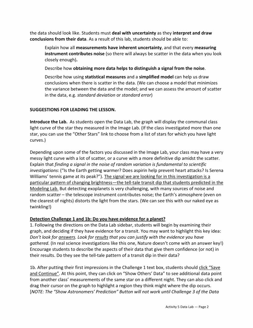
the  data  should  look  like.  Students  must  deal  with  uncertainty  as  they  interpret  and  draw  conclusions  from  their  data.  As  a  result  of  this  lab,  students  should  be  able  to:  

Explain  how  all  measurements  have  inherent  uncertainty,  and  that  every  measuring  instrument  contributes  noise  (so  there  will  always  be  scatter  in  the  data  when  you  look  closely  enough).  

Describe  how  obtaining  more  data  helps  to  distinguish  a  signal  from  the  noise.    

Describe  how  using  statistical  measures  and  a  simplified  model  can  help  us  draw  conclusions  when  there  is  scatter  in  the  data.  (We  can  choose  a  model  that  minimizes  the  variance  between  the  data  and  the  model;  and  we  can  assess  the  amount  of  scatter  in  the  data,  e.g.  standard  deviation  or  standard  error)  

 SUGGESTIONS  FOR  LEADING  THE  LESSON.    Introduce  the  Lab.    As  students  open  the  Data  Lab,  the  graph  will  display  the  communal  class  light  curve  of  the  star  they  measured  in  the  Image  Lab.  (If  the  class  investigated  more  than  one  star,  you  can  use  the  “Other  Stars”  link  to  choose  from  a  list  of  stars  for  which  you  have  light  curves.)    Depending  upon  some  of  the  factors  you  discussed  in  the  Image  Lab,  your  class  may  have  a  very  messy  light  curve  with  a  lot  of  scatter,  or  a  curve  with  a  more  definitive  dip  amidst  the  scatter.  Explain  that  finding  a  signal  in  the  noise  of  random  variation  is  fundamental  to  scientific  investigations:  (“Is  the  Earth  getting  warmer?  Does  aspirin  help  prevent  heart  attacks?  Is  Serena  Williams’  tennis  game  at  its  peak?”).  The  signal  we  are  looking  for  in  this  investigation  is  a  particular  pattern  of  changing  brightness—the  tell-­‐tale  transit  dip  that  students  predicted  in  the  Modeling  Lab.  But  detecting  exoplanets  is  very  challenging,  with  many  sources  of  noise  and  random  scatter  –  the  telescope  instrument  contributes  noise;  the  Earth’s  atmosphere  (even  on  the  clearest  of  nights)  distorts  the  light  from  the  stars.  (We  can  see  this  with  our  naked  eye  as  twinkling!)      Detection  Challenge  1  and  1b:  Do  you  have  evidence  for  a  planet?    1.  Following  the  directions  on  the  Data  Lab  sidebar,  students  will  begin  by  examining  their  graph,  and  deciding  if  they  have  evidence  for  a  transit.  You  may  want  to  highlight  this  key  idea:  Don’t  look  for  answers.  Look  for  results  that  you  can  justify  with  the  evidence  you  have  gathered.  (In  real  science  investigations  like  this  one,  Nature  doesn’t  come  with  an  answer  key!)  Encourage  students  to  describe  the  aspects  of  their  data  that  give  them  confidence  (or  not)  in  their  results.  Do  they  see  the  tell-­‐tale  pattern  of  a  transit  dip  in  their  data?    1b.  After  putting  their  first  impressions  in  the  Challenge  1  text  box,  students  should  click  “Save  and  Continue”.  At  this  point,  they  can  click  on  “Show  Others’  Data”  to  see  additional  data  point  from  another  class’  measurements  of  the  same  star  on  a  different  night.  They  can  also  click  and  drag  their  cursor  on  the  graph  to  highlight  a  region  they  think  might  where  the  dip  occurs.  [NOTE:  The  “Show  Astronomers’  Prediction”  Button  will  not  work  until  Challenge  3  of  the  Data  

    Activity  5  Data  Lab  —  Page  3  

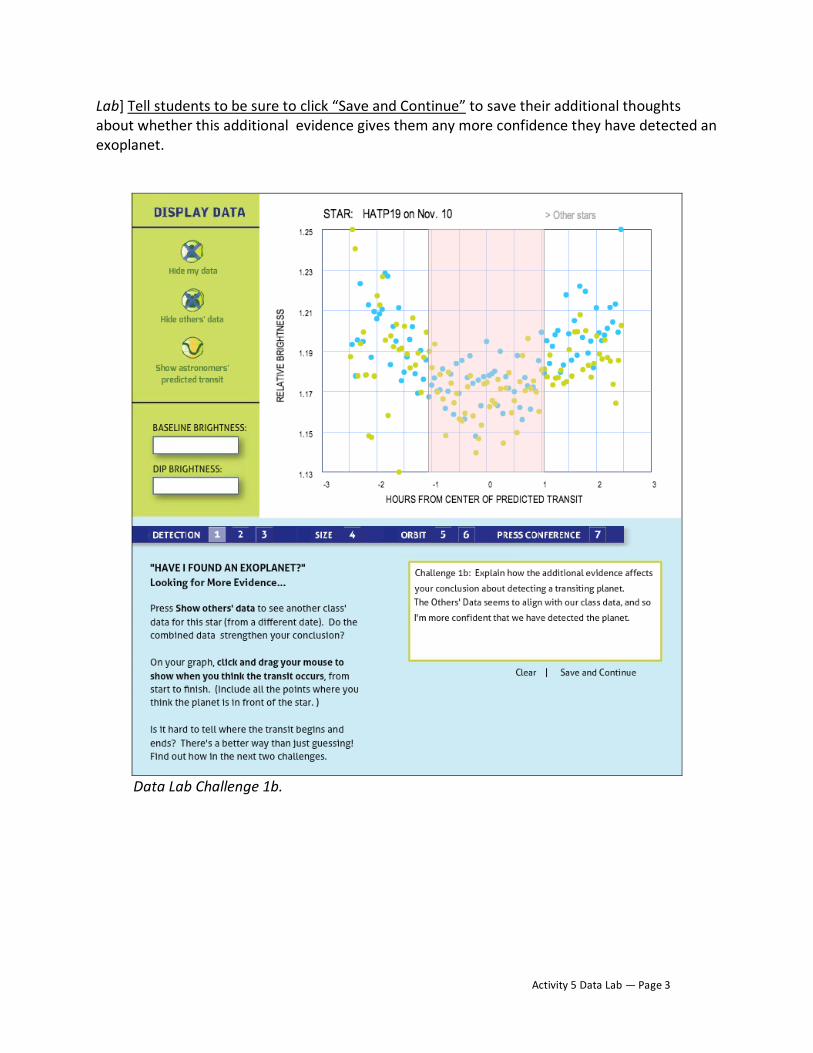
Lab]  Tell  students  to  be  sure  to  click  “Save  and  Continue”  to  save  their  additional  thoughts  about  whether  this  additional    evidence  gives  them  any  more  confidence  they  have  detected  an  exoplanet.      

    Data  Lab  Challenge  1b.

    Activity  5  Data  Lab  —  Page  4  

Detection  Challenge  2:  How  do  I  fit  a  transit  model  to  the  data?    

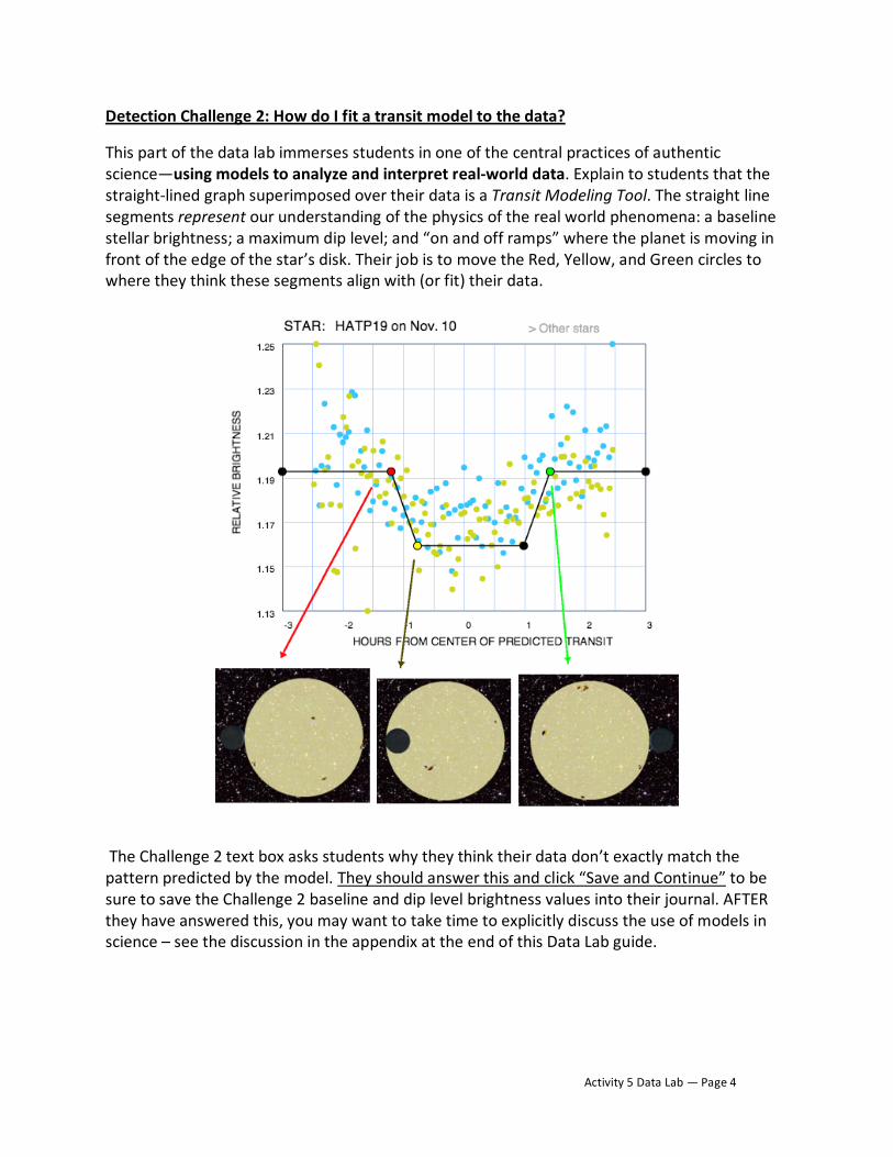
This  part  of  the  data  lab  immerses  students  in  one  of  the  central  practices  of  authentic  science—using  models  to  analyze  and  interpret  real-­‐world  data.  Explain  to  students  that  the  straight-­‐lined  graph  superimposed  over  their  data  is  a  Transit  Modeling  Tool.  The  straight  line  segments  represent  our  understanding  of  the  physics  of  the  real  world  phenomena:  a  baseline  stellar  brightness;  a  maximum  dip  level;  and  “on  and  off  ramps”  where  the  planet  is  moving  in  front  of  the  edge  of  the  star’s  disk.  Their  job  is  to  move  the  Red,  Yellow,  and  Green  circles  to  where  they  think  these  segments  align  with  (or  fit)  their  data.  

 

 The  Challenge  2  text  box  asks  students  why  they  think  their  data  don’t  exactly  match  the  pattern  predicted  by  the  model.  They  should  answer  this  and  click  “Save  and  Continue”  to  be  sure  to  save  the  Challenge  2  baseline  and  dip  level  brightness  values  into  their  journal.  AFTER  they  have  answered  this,  you  may  want  to  take  time  to  explicitly  discuss  the  use  of  models  in  science  –  see  the  discussion  in  the  appendix  at  the  end  of  this  Data  Lab  guide.  

 

 

    Activity  5  Data  Lab  —  Page  5  

Detection  Challenge  3:  Which  transit  model  best  fits  my  data?    

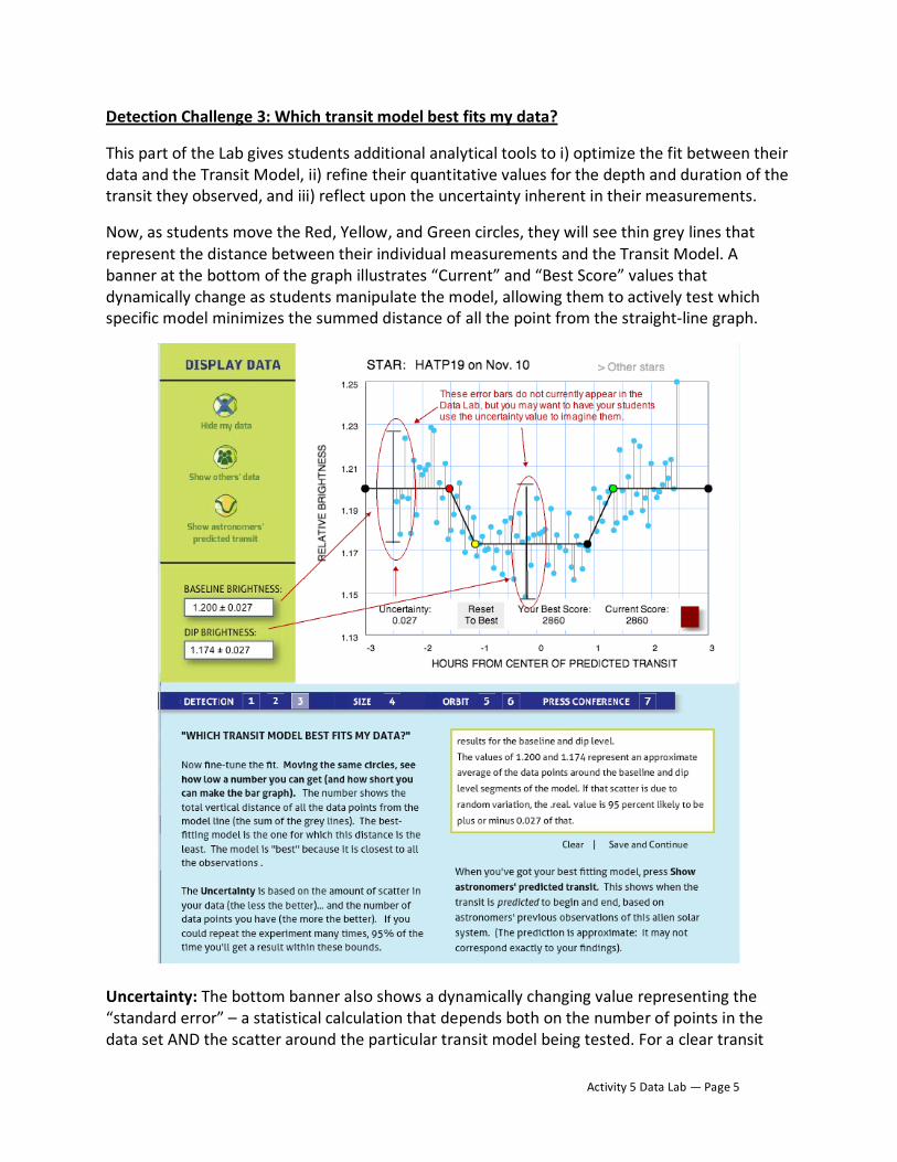
This  part  of  the  Lab  gives  students  additional  analytical  tools  to  i)  optimize  the  fit  between  their  data  and  the  Transit  Model,  ii)  refine  their  quantitative  values  for  the  depth  and  duration  of  the  transit  they  observed,  and  iii)  reflect  upon  the  uncertainty  inherent  in  their  measurements.  

Now,  as  students  move  the  Red,  Yellow,  and  Green  circles,  they  will  see  thin  grey  lines  that  represent  the  distance  between  their  individual  measurements  and  the  Transit  Model.  A  banner  at  the  bottom  of  the  graph  illustrates  “Current”  and  “Best  Score”  values  that  dynamically  change  as  students  manipulate  the  model,  allowing  them  to  actively  test  which  specific  model  minimizes  the  summed  distance  of  all  the  point  from  the  straight-­‐line  graph.  

   Uncertainty:  The  bottom  banner  also  shows  a  dynamically  changing  value  representing  the  “standard  error”  –  a  statistical  calculation  that  depends  both  on  the  number  of  points  in  the  data  set  AND  the  scatter  around  the  particular  transit  model  being  tested.  For  a  clear  transit  

    Activity  5  Data  Lab  —  Page  6  

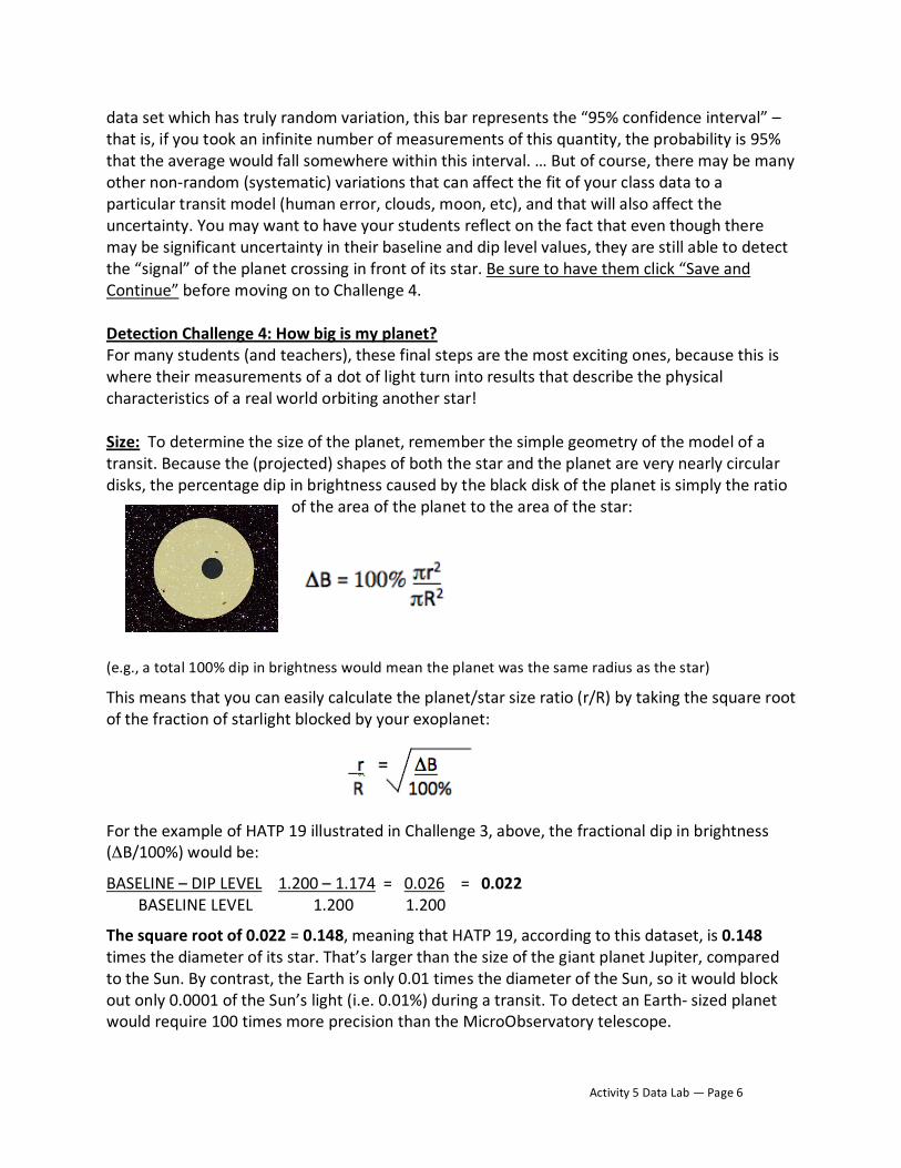
data  set  which  has  truly  random  variation,  this  bar  represents  the  “95%  confidence  interval”  –  that  is,  if  you  took  an  infinite  number  of  measurements  of  this  quantity,  the  probability  is  95%  that  the  average  would  fall  somewhere  within  this  interval.  …  But  of  course,  there  may  be  many  other  non-­‐random  (systematic)  variations  that  can  affect  the  fit  of  your  class  data  to  a  particular  transit  model  (human  error,  clouds,  moon,  etc),  and  that  will  also  affect  the  uncertainty.  You  may  want  to  have  your  students  reflect  on  the  fact  that  even  though  there  may  be  significant  uncertainty  in  their  baseline  and  dip  level  values,  they  are  still  able  to  detect  the  “signal”  of  the  planet  crossing  in  front  of  its  star.  Be  sure  to  have  them  click  “Save  and  Continue”  before  moving  on  to  Challenge  4.    Detection  Challenge  4:  How  big  is  my  planet?    For  many  students  (and  teachers),  these  final  steps  are  the  most  exciting  ones,  because  this  is  where  their  measurements  of  a  dot  of  light  turn  into  results  that  describe  the  physical  characteristics  of  a  real  world  orbiting  another  star!    Size:    To  determine  the  size  of  the  planet,  remember  the  simple  geometry  of  the  model  of  a  transit.  Because  the  (projected)  shapes  of  both  the  star  and  the  planet  are  very  nearly  circular  disks,  the  percentage  dip  in  brightness  caused  by  the  black  disk  of  the  planet  is  simply  the  ratio  

of  the  area  of  the  planet  to  the  area  of  the  star:                                    

 (e.g.,  a  total  100%  dip  in  brightness  would  mean  the  planet  was  the  same  radius  as  the  star) This  means  that  you  can  easily  calculate  the  planet/star  size  ratio  (r/R)  by  taking  the  square  root  of  the  fraction  of  starlight  blocked  by  your  exoplanet:    

         

For  the  example  of  HATP  19  illustrated  in  Challenge  3,  above,  the  fractional  dip  in  brightness  (ΔB/100%)  would  be:    

BASELINE  –  DIP  LEVEL        1.200  –  1.174    =      0.026        =      0.022                    BASELINE  LEVEL                          1.200                          1.200  

The  square  root  of  0.022  =  0.148,  meaning  that  HATP  19,  according  to  this  dataset,  is  0.148  times  the  diameter  of  its  star.  That’s  larger  than  the  size  of  the  giant  planet  Jupiter,  compared  to  the  Sun.  By  contrast,  the  Earth  is  only  0.01  times  the  diameter  of  the  Sun,  so  it  would  block  out  only  0.0001  of  the  Sun’s  light  (i.e.  0.01%)  during  a  transit.  To  detect  an  Earth-­‐  sized  planet  would  require  100  times  more  precision  than  the  MicroObservatory  telescope.    

    Activity  5  Data  Lab  —  Page  7  

 

To  enter  the  correct  value  in  the  SIZE  textbox,  students  should  use  their  values  for  “baseline”  and  “dip”  brightness  and  follow  these  4  steps:  

1.    BASELINE  BRIGHTNESS  LEVEL  FROM  CHALLENGE  3            ______  

2.    DIP  LEVEL  BRIGHTNESS    LEVEL  FROM  CHALLENGE  3        ______  

3.    PERCENTAGE  DIP,    ΔB/100%  =  (1.  –  2.)/1.  :      _______  

4.    SIZE  RATIO  OF  PLANET/STAR,    r/R  =  sqrt(3.):        _______  

Enter  the  result  from  Step  4  into  the  textbox  in  Challenge  4,  and  click  “Save  and  Continue”  to  save  this  value  into  the  Journal.      Detection  Challenge  5:  Is  the  planet’s  orbit  tilted?    In  order  to  even  see  a  transit,  the  orbit  must  be  fairly  “Edge-­‐On”  with  respect  to  our  view  from  Earth.  Transits  for  most  of  the  stars  have  a  flat  “trough”,  indicating  that  the  planet’s  orbit  is  nearly  90  degrees  edge-­‐on,  and  the  planet  transits  across  the  middle  of  the  main  face  of  the  star.  But  for  the  star  TrES3,  for  example,  the  planet’s  orbit  is  tilted  8%  from  an  edge-­‐on  view  (it  has  an  “inclination”  of  82  degrees),  so  the  transiting  disk  of  the  planet  just  grazes  the  star.  The  transit  graph  looks  more  like  a  “V”:  As  soon  as  there  is  a  dip,  the  brightness  returns  to  the  baseline  level.  The  precision  of  students’  data  should  typically  allow  them  to  identify  whether  their  observations  indicate  a  more  edge-­‐on,  or  more  tilted,  orbital  plane.  Have  students  click  on  the  graph  image  that  represents  their  choice,  and  then  click  “Save  and  Continue”.  

 Detection  Challenge  6:  How  close  is  the  planet  to  its  star?    For  this  final  important  planetary  characteristic,  you’ll  use  Kepler’s  3rd  Law,  the  mathematical  relationship  that  describes  how  the  closer  a  planet  is  to  its  star,  the  faster  it  moves—and  so  the  shorter  its  transit  time.      Typically,  Kepler’s  law  is  expressed  as  a  relationship  between  the  period  (T)  of  the  planet  (it’s  year,  or  Time  for  one  orbit),  and  the  “semi-­‐major  axis”  of  its  elliptical  orbit,  which  for  a  circular  orbit,  is  simply  R,  the  distance  between  the  star  and  planet.  Kepler  discovered  that  R3  =  T2,  where  R  is  expressed  in  Astronomical  Units  (AU,  the  average  Earth-­‐Sun  distance),  and  T  in  units  of  “Earth”  years.        In  this  calculation,  you  and  your  students  will  assume  a  circular  orbit,  and  also  assume  that  the  target  star  is  Sun-­‐like  (the  same  mass  and  diameter),  so  that  you  can  directly  compare  the  orbital  speed  and  distance  of  your  exoplanet  with  that  of  the  Earth.  (Of  course  your  result  will  then  only  be  approximate  if  the  target  star  is  not  the  same  mass  or  diameter  of  the  Sun.)  

    Activity  5  Data  Lab  —  Page  8  

 Using  Transit  Duration  and  Orbital  Speed  to  Determine  Planetary  Distance  R  While  your  class  typically  will  not  know  the  period  (T)  of  their  planet  (they  would  have  to  observe  at  least  2  transits  in  a  row  to  determine  this),  they  DO  have  the  transit  duration,  which,  as  a  measure  of  the  planet’s  orbital  speed,  is  proportional  to  the  square  root  of  its  orbital  distance  from  its  star  (longer  duration  transits  mean  larger  orbital  distances).    Challenge  6  Textbox:  Your  students  can  “read  off”  the  orbital  distance  of  their  planet  from  the  graphical  chart  on  the  page.  For  more  math-­‐based  courses,  you  might  choose  to  have  students  calculate  their  planet’s  orbital  speed  and  then  substitute  that  into  Kepler’s  Law  to  calculate  the  orbital  distance.  If  the  exoplanet  transits  the  star  in,  say,  3  hours,  then  its  approximate  speed  (v)  is  simply  the  diameter  of  a  Sun-­‐like  star  (1.4  million  km)  divided  by  the  transit  duration  (3  hrs)  =  467,000  km/hr.    By  comparing  this  orbital  speed  with  the  Earth’s  orbital  speed  (about  100,000  km/hr)    Here’s  how  to  use  orbital  speed,  v,  in  Kepler’s  equation  rather  than  the  period,  T:    It  should  be  straightforward  to  see  that  the  period  (T)  times  the  orbital  speed  (v)  equals  the  orbital  circumference  2πR,  so  that  T  =  2πR/v.    Substituting  this  in  to  Kepler’s  equation  R3  =  T2,  we  have:                                              R3  =  4π2R2                                          v2  Now,  you  can  see  that  the  distance  R  is  proportional  to  1/v2  So….  if  your  exoplanet’s  orbital  speed  is  4.7  times  that  of  the  Earth  (as  above),  then  its  distance  from  its  star  is  1/(4.7)2  or  0.045  AU!    The  importance  of  this  distance  is  that  it  bears  on  whether  the  planet  might  be  habitable.  The  planets  detected  in  this  project  are  all  very  close  to  their  stars.  Liquid  water  would  not  exist  on  these  planets,  and  neither  would  life.  

 Detection  Challenge  7:  Publish  your  results  and  prepare  a  press  conference  briefing!!    Don’t  forget  to  reflect  on  what  is  amazing  about  this  Lab:    Your  class  was  able  to  detect  a  planet  and  tell  something  about  it,  just  from  measuring  the  starlight!    This  last  page  of  the  DataLab  provides  an  opportunity  for  students  to  reflect  upon  and  sum  up  their  finding  through  the  whole  investigation.  They  can  open  up  their  journal  to  refresh  their  memory  about  all  the  steps  they  went  through  as  the  prepare  the  text  for  this  last  step  of  the  Data  Lab.