Embed Size (px)
Citation preview

Free University of Bolzano–Database 2. Lecture IV, 2003/2004 – A.Artale (1)
Databases 2Lecture IV
Alessandro ArtaleFaculty of Computer Science – Free University of Bolzano
Room: 221
http://www.inf.unibz.it/ �artale/
2003/2004 – First Semester

Free University of Bolzano–Database 2. Lecture IV, 2003/2004 – A.Artale (2)
Summary of Lecture IV
� Query Compilation and Optimization
� Algorithms for Implementing Query Operators
– One-Pass Algorithms
– One-And-A-Half Passes Algorithms
� Nested-Loop Join
– Two-Pass Algorithms
� Sort-Based Algorithms
� Index-Based Algorithms.

Free University of Bolzano–Database 2. Lecture IV, 2003/2004 – A.Artale (3)
Query Compilation Overview
SQL query
Parsing
Query Rewriting
Plan Generation
Execute Plan
query parse tree
logical query plan tree
physical query plan tree

Free University of Bolzano–Database 2. Lecture IV, 2003/2004 – A.Artale (4)
Query Optimization
� Crucial for query optimization are both the query rewriting and the plan
generation phases.
� To select the best query plan decision involve:
1. Choose the best algorithm for implementing each of the operations of the
logical query plan;
2. Choose the logical query plan that leads to the most efficient algorithm
for answering the query.
� Each of these choices depend on:
1. The size of the relations involved;
2. Existence of indexes on the relations;
3. Layout of data on disk.

Free University of Bolzano–Database 2. Lecture IV, 2003/2004 – A.Artale (5)
Cost of Physical-Query-Plan Operators
� Physical-Query-Plan Operators implement both relational algebra opera-
tors, and generic operations like the scan of a relation – to bring into main
memory all the tuples of a relation – or the sort of a relation.
� The Cost associated to the execution of each operator is based on the number
of disk I/O – as specified by the I/O Model of Computation.
� For estimating the cost of an operator the following parameters are used:
1. M: The number of main memory buffers (assumed equal in size to a disk
block) available during the execution of an operator;
2. Parameters that measure size and distribution of data in relations:
(a) B(R): number of blocks holding the relation
�
– if a relation is
clustered, i.e., stored in fully dedicated blocks, then B(R) measures the
cost of scanning the relation;
(b) T(R): number of tuples in
�
;
(c) V(R,A): number of distinct values for the attribute
�
of the relation
�
.
Free University of Bolzano–Database 2. Lecture IV, 2003/2004 – A.Artale (6)
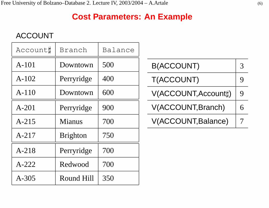
Cost Parameters: An Example
ACCOUNT
Account
�
Branch Balance
A-101 Downtown 500
A-102 Perryridge 400
A-110 Downtown 600
A-201 Perryridge 900
A-215 Mianus 700
A-217 Brighton 750
A-218 Perryridge 700
A-222 Redwood 700
A-305 Round Hill 350
B(ACCOUNT) 3
T(ACCOUNT) 9
V(ACCOUNT,Account
�
) 9
V(ACCOUNT,Branch) 6
V(ACCOUNT,Balance) 7

Free University of Bolzano–Database 2. Lecture IV, 2003/2004 – A.Artale (7)
Summary
� Query Compilation and Optimization
� Algorithms for Implementing Operators
– One-Pass Algorithms
– One-And-A-Half Passes Algorithms
� Nested-Loop Join
– Two-Pass Algorithms
� Sort-Based Algorithms
� Index-Based Algorithms.

Free University of Bolzano–Database 2. Lecture IV, 2003/2004 – A.Artale (8)
Classification of Operators
Operators can be classified into three classes:
1. Tuple-at-a-time, unary operators. Operators that do not require whole
relation in main memory – selection, projection.
2. Full-relation, unary operators. Operators that require whole relation in
main memory – ���
�
.
3. Full-relation, binary operators. At least one of the involved relations
should reside in main memory – all the remaining operators belong to this
class.
Free University of Bolzano–Database 2. Lecture IV, 2003/2004 – A.Artale (9)
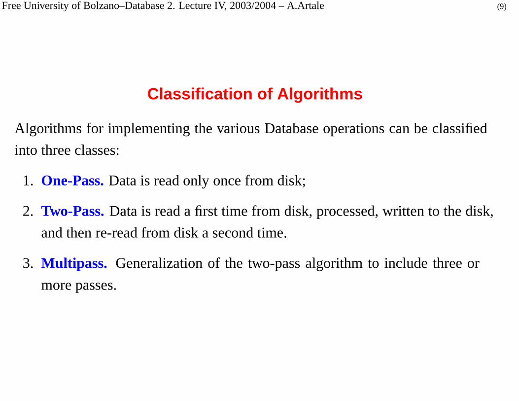
Classification of Algorithms
Algorithms for implementing the various Database operations can be classified
into three classes:
1. One-Pass. Data is read only once from disk;
2. Two-Pass. Data is read a first time from disk, processed, written to the disk,
and then re-read from disk a second time.
3. Multipass. Generalization of the two-pass algorithm to include three or
more passes.

Free University of Bolzano–Database 2. Lecture IV, 2003/2004 – A.Artale (10)
Summary
� Query Compilation and Optimization
� Algorithms for Implementing Operators
– One-Pass Algorithms
– One-And-A-Half Passes Algorithms
� Nested-Loop Join
– Two-Pass Algorithms
� Sort-Based Algorithms
� Index-Based Algorithms.

Free University of Bolzano–Database 2. Lecture IV, 2003/2004 – A.Artale (11)
One-Pass Algorithms for Tuple-at-Time Operators
Algorithm for Selection, �� � � �
, and Projection, �� � � �
.
1. Read the blocks of
�
one at a time into a memory buffer;
2. Perform the desired operation on the current tuples;
3. Move the selected/projected tuples on the output buffer.
Cost Analysis
� The algorithm requires that
� � �.
� The disk I/O cost is B(R).
� Note: The cost can be reduced in the case of a Selection with a condition on
an attribute that has an index (see slide 56)

Free University of Bolzano–Database 2. Lecture IV, 2003/2004 – A.Artale (12)
One-Pass Algorithms for Full-Relation, Unary Operators– Duplicate Elimination –
Algorithm for Duplicate Elimination
� � � �
.
� Read each block of
�
one at a time, and for every tuple:
1. If is the first time the tuple is seen: Copy the tuple to the output;
2. Otherwise: Do not output the tuple.
� One copy of every tuple already seen has to be kept in main memory – this is
why we have a Full-Relation algorithm – to make the above decision.

Free University of Bolzano–Database 2. Lecture IV, 2003/2004 – A.Artale (13)
One-Pass Algorithms for Full-Relation, Unary Operators– Duplicate Elimination (cont.) –
� Problem.
If we have � tuples, deciding whether a new tuple is among them takes a
time proportional to �. The full operation takes time proportional to � �
.
� Solution.
Using appropriate structures to memorize the already seen tuples: A
Balanced Binary Tree requires
��� � � to locate a tuple, then the full process
takes time proportional to � �� � �.
Cost Analysis
� The algorithm requires that� � � � � � � � �
.
� The disk I/O cost is B(R).

Free University of Bolzano–Database 2. Lecture IV, 2003/2004 – A.Artale (14)
One-Pass Algorithms for Full-Relation, Binary Operators– Cartesian Product –
Computing
� � �
– assuming that
�
is smaller in size.
� Read the whole
�
into main memory (no special structure is needed);
� Read into another buffer one block of
�
at a time;
� For each tuple
� � �
concatenate
�
with each tuple of
�
;
� Output each concatenated tuple.
Cost Analysis
� Number of memory buffers required:
� � � � � � � �� ��
� �� � � � �
.
� The disk I/O cost is B(R) + B(S);
� Considerable amount of CPU time to concatenate tuples.

Free University of Bolzano–Database 2. Lecture IV, 2003/2004 – A.Artale (15)
Cartesian Product Algorithm: An Example
STUDENT
StudID
�
Name Course
123 John CS
142 Marc CS
154 Mary Maths
221 Judi Physics�
ACCOUNT
Acc
�
Branch Balance
A-101 Downtown 500
A-102 Perryridge 400
A-110 Downtown 600
A-201 Perryridge 900
A-215 Mianus 700
A-217 Brighton 750
A-218 Perryridge 700
A-222 Redwood 700
A-305 Round Hill 350

Free University of Bolzano–Database 2. Lecture IV, 2003/2004 – A.Artale (16)
Cartesian Product Algorithm: An Example (Cont.)
� Cycle 1: The first block of ACCOUNT is brought in Main Memory.
MAIN MEMORY OUTPUT
STUDENT
123 John CS
142 Marc CS
154 Mary Maths
221 Judi Physics
ACCOUNT (
� � �
Block)
A-101 Downtown 500
A-102 Perryridge 400
A-110 Downtown 600
STUDENT � ACCOUNT(Cycle 1)
StudID
�
Name Course Acc�
Branch Balance
123 John CS A-101 Downtown 500
123 John CS A-102 Perryridge 400
123 John CS A-110 Downtown 600
142 Marc CS A-101 Downtown 500
142 Marc CS A-102 Perryridge 400
142 Marc CS A-110 Downtown 600
154 Mary Maths A-101 Downtown 500
154 Mary Maths A-102 Perryridge 400
154 Mary Maths A-110 Downtown 600
221 Judi Physics A-101 Downtown 500
221 Judi Physics A-102 Perryridge 400
221 Judi Physics A-110 Downtown 600

Free University of Bolzano–Database 2. Lecture IV, 2003/2004 – A.Artale (17)
Cartesian Product Algorithm: An Example (Cont.)
� Cycle 2: The second block of ACCOUNT is brought in Main Memory.
MAIN MEMORY OUTPUT
STUDENT
123 John CS
142 Marc CS
154 Mary Maths
221 Judi Physics
ACCOUNT (
� � �
Block)
A-201 Perryridge 900
A-215 Mianus 700
A-217 Brighton 750
STUDENT � ACCOUNT(Cycle 2)
StudID
�
Name Course Acc�
Branch Balance
123 John CS A-201 Perryridge 900
123 John CS A-215 Mianus 700
123 John CS A-217 Brighton 750
142 Marc CS A-201 Perryridge 900
142 Marc CS A-215 Mianus 700
142 Marc CS A-217 Brighton 750
154 Mary Maths A-201 Perryridge 900
154 Mary Maths A-215 Mianus 700
154 Mary Maths A-217 Brighton 750
221 Judi Physics A-201 Perryridge 900
221 Judi Physics A-215 Mianus 700
221 Judi Physics A-217 Brighton 750

Free University of Bolzano–Database 2. Lecture IV, 2003/2004 – A.Artale (18)
Cartesian Product Algorithm: An Example (Cont.)
� Cycle 3: The third block of ACCOUNT is brought in Main Memory.
MAIN MEMORY OUTPUT
STUDENT
123 John CS
142 Marc CS
154 Mary Maths
221 Judi Physics
ACCOUNT (
� � �
Block)
A-218 Perryridge 700
A-222 Redwood 700
A-305 Round Hill 350
STUDENT � ACCOUNT(Cycle 3)
StudID
�
Name Course Acc�
Branch Balance
123 John CS A-218 Perryridge 700
123 John CS A-222 Redwood 700
123 John CS A-305 Round Hill 350
142 Marc CS A-218 Perryridge 700
142 Marc CS A-222 Redwood 700
142 Marc CS A-305 Round Hill 350
154 Mary Maths A-218 Perryridge 700
154 Mary Maths A-222 Redwood 700
154 Mary Maths A-305 Round Hill 350
221 Judi Physics A-218 Perryridge 700
221 Judi Physics A-222 Redwood 700
221 Judi Physics A-305 Round Hill 350

Free University of Bolzano–Database 2. Lecture IV, 2003/2004 – A.Artale (19)
One-Pass Algorithms for Full-Relation, Binary Operators– Natural Join –
Computing
� � ��
� � � � � ��
� �
–
��
��
�
are set of attributes.
� Read the whole
�
into a main memory search structure (Balanced Binary
Trees), with
�
as a search key;
� Read into another buffer one block of
�
at a time;
� For each tuple
� � �
search all the tuples in
�that agree with
�
on the value
of
�
, using the search structure;
� Join such tuples (concatenation with only one repetition of the
�
attributes),
and then output them.
Cost Analysis
� Number of memory buffers required:
� � � � � � � �� ��
� �� � � � �
.
� The disk I/O cost is� �� � � � �� �
;
� Considerable amount of CPU time to concatenate tuples.

Free University of Bolzano–Database 2. Lecture IV, 2003/2004 – A.Artale (20)
Natural Join Algorithm: An Example
Assume that three tuples fit in one block.
BRANCH
BName SortCode Phone
Downtown 156432 01636754
Perryridge 452341 01436754
Mianus 335699 01994545
Brighton 657841 01227676
Redwood 521775 01336546
Round Hill 903215 01764008
�
ACCOUNT
Acc
�
BName Balance
A-101 Downtown 500
A-102 Perryridge 400
A-110 Downtown 600
A-201 Perryridge 900
A-215 Mianus 700
A-217 Brighton 750
A-218 Perryridge 700
A-222 Redwood 700
A-305 Round Hill 350

Free University of Bolzano–Database 2. Lecture IV, 2003/2004 – A.Artale (21)
Natural Join Algorithm: An Example (Cont.)
� Cycle 1: The first block of ACCOUNT is brought in Main Memory.
MAIN MEMORY OUTPUTBRANCH
Downtown 156432 01636754
Perryridge 452341 01438300
Mianus 335699 01994545
Brighton 657841 01227676
Redwood 521775 01336546
Round Hill 903215 01764008
ACCOUNT (
� � �
Block)
A-101 Downtown 500
A-102 Perryridge 400
A-110 Downtown 600
BRANCH
�
ACCOUNT(Cycle 1)
BName SortCode Phone Acc
�
Balance
Downtown 156432 01636754 A-101 500
Downtown 156432 01636754 A-110 600
Perryridge 452341 01438300 A-102 400

Free University of Bolzano–Database 2. Lecture IV, 2003/2004 – A.Artale (22)
Natural Join Algorithm: An Example (Cont.)
� Cycle 2: The second block of ACCOUNT is brought in Main Memory.
MAIN MEMORY OUTPUTBRANCH
Downtown 156432 01636754
Perryridge 452341 01438300
Mianus 335699 01994545
Brighton 657841 01227676
Redwood 521775 01336546
Round Hill 903215 01764008
ACCOUNT (
� � �
Block)
A-201 Perryridge 900
A-215 Mianus 700
A-217 Brighton 750
BRANCH
�
ACCOUNT(Cycle 2)
BName SortCode Phone Acc
�
Balance
Perryridge 452341 01438300 A-201 900
Mianus 335699 01994545 A-215 700
Brighton 657841 01227676 A-217 750

Free University of Bolzano–Database 2. Lecture IV, 2003/2004 – A.Artale (23)
Natural Join Algorithm: An Example (Cont.)
� Cycle 3: The third block of ACCOUNT is brought in Main Memory.
MAIN MEMORY OUTPUTBRANCH
Downtown 156432 01636754
Perryridge 452341 01438300
Mianus 335699 01994545
Brighton 657841 01227676
Redwood 521775 01336546
Round Hill 903215 01764008
ACCOUNT (
� � �
Block)
A-218 Perryridge 700
A-222 Redwood 700
A-305 Round Hill 350
BRANCH
�
ACCOUNT(Cycle 3)
BName SortCode Phone Acc
�
Balance
Perryridge 452341 01438300 A-218 700
Redwood 521775 01336546 A-222 700
Round Hill 903215 01764008 A-305 350

Free University of Bolzano–Database 2. Lecture IV, 2003/2004 – A.Artale (24)
Summary
� Query Compilation and Optimization
� Algorithms for Implementing Operators
– One-Pass Algorithms
– One-And-A-Half Passes Algorithms
� Nested-Loop Join
– Two-Pass Algorithms
� Sort-Based Algorithms
� Index-Based Algorithms.

Free University of Bolzano–Database 2. Lecture IV, 2003/2004 – A.Artale (25)
Nested-Loop Join
� Algorithms with “One-And-A-Half”-passes: Used when relations don’t fit
in main memory (which is the common situation in real Databases).
� One of the arguments is read only once, while the other is read more times.

Free University of Bolzano–Database 2. Lecture IV, 2003/2004 – A.Artale (26)
Nested-Loop Join (cont.)
Computing
� � �
using a tuple-based nested-loop join algorithm, with�
smaller
in size – a naive way to implement join.
TUPLE-BASED-NESTED-LOOP-JOIN(
��
�
)
FOR each tuple � of
�
DO
FOR each tuple � of
�
DO
IF � and � join THEN
output the resulting tuple;
Cost Analysis
� If we buffer each relation one block at a time:
Number of Disk I/O:
� �� � � � �� � � � �� �
.
� Example. Let
� � � �� ��
� � ��
� � � �� � � ��
� � � �� ��
� � �
, then:
ONE-PASS JOIN costs� � � � � � � � �
� ��
� � �
disk I/O;
TUPLE-BASED NESTED-LOOP JOIN costs
� � � � � � � � � � � � � ��
��
� � ��
� � �
disk I/O.

Free University of Bolzano–Database 2. Lecture IV, 2003/2004 – A.Artale (27)
Block-Based Nested-Loop Join
Optimize the TUPLE-BASED NESTED-LOOP JOIN algorithm.
Use as much main memory as we can to store
�
, i.e., if�
are the available
memory buffers we reserve
��� �
buffers to
�
and
�
to�
.
BLOCK-BASED-NESTED-LOOP-JOIN(
��
�
)
FOR each chunk of
�� �
blocks of�
DO
read them to a main-memory search structure
with the common attributes as search key;
FOR each tuple � of�
DO
search the current tuples of
�
that join with �;
output the resulting joining tuples;
Free University of Bolzano–Database 2. Lecture IV, 2003/2004 – A.Artale (28)
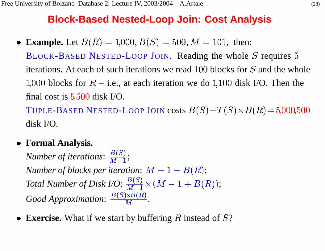
Block-Based Nested-Loop Join: Cost Analysis
� Example. Let
� � � �� ��
� � ��
� � � �� � � ��
� � � � �
, then:
BLOCK-BASED NESTED-LOOP JOIN. Reading the whole�
requires
�
iterations. At each of such iterations we read
� � �
blocks for�
and the whole
��
� � �
blocks for
�
– i.e., at each iteration we do
��
� � �disk I/O. Then the
final cost is
��
� � �
disk I/O.
TUPLE-BASED NESTED-LOOP JOIN costs
� � � � � � � � � � � � � �� ��
� � ��
� � �
disk I/O.
� Formal Analysis.
Number of iterations:
� �� ���� � ;
Number of blocks per iteration:�� � � � � � �
;
Total Number of Disk I/O:� �� �
�� � � � ��� � � � � � � �
;
Good Approximation:� �� �� � � �
� .
� Exercise. What if we start by buffering
�
instead of
�
?

Free University of Bolzano–Database 2. Lecture IV, 2003/2004 – A.Artale (29)
Summary
� Query Compilation and Optimization
� Algorithms for Implementing Operators
– One-Pass Algorithms
– One-And-A-Half Passes Algorithms
� Nested-Loop Join
– Two-Pass Algorithms
� Sort-Based Algorithms
� Index-Based Algorithms.

Free University of Bolzano–Database 2. Lecture IV, 2003/2004 – A.Artale (30)
Two-Pass Algorithms Based on Sorting
Two- or Multi-Pass Algorithms are used when full relations do not fit in main
memory – which is the norm for large databases.
� General Idea. Given a relation with
� � � � � �
then:
1. Read
�
blocks of
�
into main memory;
2. Sort these
�
blocks in main memory using efficient structures – for
Balanced Binary Trees sorting � elements costs � �� � �.
3. Write the sorted buffers into
�
disk blocks, called sorted sublist of
�
.
Go to step 1 if there are unconsidered blocks for R.
4. Use a Second Pass to “merge” the sorted sublists for computing the final
result.
� Steps 1,2,3 above form the common First Pass in a Two-Pass algorithm
based on sorting.

Free University of Bolzano–Database 2. Lecture IV, 2003/2004 – A.Artale (31)
Two-Pass Algorithms Based on Sorting– Natural Join –
Computing
� � ��
� � � � � ��
� �
with a sort-based algorithm:
1. “Sort”
�
and
�
by
�
if they are not already sorted;
2. “Merge” the sorted relations matching all tuples with common values of
�
:
(a) Read the current block of both
�
and
�
in main memory;
(b) Find the tuple with the least value � for
�
;
(c) If � does not appear at the front of the other relation then consider the
successive least �;
(d) Otherwise, identify ALL tuples from BOTH relations having sort key �.
Note. If necessary read subsequent blocks from
�
and/or
�
to find
ALL tuples with search key �. If more than the
�
available buffers are
necessary the algorithm doesn’t work anymore.
(e) Output the joining tuples;
(f) If either relation has no more unconsidered tuples in main memory, reload
the buffer for this relation, and go back to step 2b.

Free University of Bolzano–Database 2. Lecture IV, 2003/2004 – A.Artale (32)
Sort-Based Natural Join: Example
Suppose that three tuples fit on a block, and the sorted relations (w.r.t. BName)
are:
BRANCH
BName SortCode Phone
Brighton 657841 01227676
Downtown 156432 01636754
Mianus 335699 01994545
Perryridge 452341 01436754
Redwood 521775 01336546
Round Hill 903215 01764008
�
ACCOUNT
Acc
�
BName Balance
A-217 Brighton 750
A-101 Downtown 500
A-110 Downtown 600
A-215 Mianus 700
A-102 Perryridge 400
A-201 Perryridge 900
A-218 Perryridge 700
A-222 Redwood 700
A-305 Round Hill 350

Free University of Bolzano–Database 2. Lecture IV, 2003/2004 – A.Artale (33)
Sort-Based Natural Join: Example (Cont.)
� Cycle 1: The first block of both BRANCH and ACCOUNT are brought in
Main Memory. MAIN MEMORY
BRANCH
BName SortCode Phone
Brighton 657841 01227676
Downtown 156432 01636754
Mianus 335699 01994545
�
ACCOUNT
Acc
�
BName Balance
A-217 Brighton 750
A-101 Downtown 500
A-110 Downtown 600
OUTPUT
BRANCH
�
ACCOUNT(Cycle 1)
BName SortCode Phone Acc
�
Balance
Brighton 657841 01227676 A-217 750
Downtown 156432 01636754 A-101 500
Downtown 156432 01636754 A-110 600

Free University of Bolzano–Database 2. Lecture IV, 2003/2004 – A.Artale (34)
Sort-Based Natural Join: Example (Cont.)
� Cycle 2: The second block of ACCOUNT is brought in Main Memory.
MAIN MEMORY
BRANCH
BName SortCode Phone
Brighton 657841 01227676
Downtown 156432 01636754
Mianus 335699 01994545�
ACCOUNT
Acc
�
BName Balance
A-215 Mianus 700
A-102 Perryridge 400
A-201 Perryridge 900
OUTPUT
BRANCH
�
ACCOUNT(Cycle 2)
Mianus 335699 01994545 A-215 700

Free University of Bolzano–Database 2. Lecture IV, 2003/2004 – A.Artale (35)
Sort-Based Natural Join: Example (Cont.)
� Cycle 3: The second block of BRANCH and the third of ACCOUNT are
brought in Main Memory.
MAIN MEMORY
BRANCH
BName SortCode Phone
Perryridge 452341 01436754
Redwood 521775 01336546
Round Hill 903215 01764008
�
ACCOUNT
Acc�
BName Balance
A-215 Mianus 700
A-102 Perryridge 400
A-201 Perryridge 900
A-218 Perryridge 700
A-222 Redwood 700
A-305 Round Hill 350

Free University of Bolzano–Database 2. Lecture IV, 2003/2004 – A.Artale (36)
Sort-Based Natural Join: Example (Cont.)
OUTPUT(Cycle 3)
BRANCH
�
ACCOUNT(Cycle 3)
Perryridge 452341 01438300 A-102 400
Perryridge 452341 01438300 A-201 900
Perryridge 452341 01438300 A-218 700
Redwood 521775 01336546 A-222 700
Round Hill 903215 01764008 A-305 350

Free University of Bolzano–Database 2. Lecture IV, 2003/2004 – A.Artale (37)
Sort-Based Natural Join: Cost Analysis
� Number of Disk I/O:
� � � � � � � � � � � � �
.
1. Sorting with a two-phase merge sort algorithm costs�
disk I/O per block.
Then the sorting phase requires
� � � � � � � � � � � � �
disk I/O.
2. The merge-join phase requires reading each block of the involved
relations one time. Thus, this phase costs� � � � � � � � � � �
disk I/O.
3. Total Cost:
� � � � � � � � � � � � �disk I/O.
� Number of memory buffer required:
� � max
� � � � ��
� � � � �
.
– Needed to perform the sort.

Free University of Bolzano–Database 2. Lecture IV, 2003/2004 – A.Artale (38)
Sort-Based Join: Cost Analysis (cont.)
� Example. Let
� � � �� � � � ��
� � � �� � � ��
� � � � �
, and for no � do the
tuples of
�
and
�
that agree on � occupy more than
� � �
blocks, then the cost
of different techniques are:
Sort-Based Join:
� � � � � � � � � � � � �� ��
� � �
disk I/O.
Block-Based Nested-Loop Join:
� �� ��� � � � �� � � � � � � �
� ��
� � �
disk I/O.
Tuple-Based Nested-Loop Join:
� � � � � � � � � � � � � �� ��
� � ��
� � �
disk I/O.
� Note. The cost of BLOCK-BASED NESTED-LOOP JOIN grows following a
quadratic function – proportional to� � � � � � � � �
– while SORT-BASED
JOIN grows linearly – proportional to
� � � � � � � � �
. Then SORT-BASED
JOIN is a better performing algorithm as far as the size of the relations grows.
– Indeed, try with:� � � �
� � ��
� � ��
� � � �� ��
� � ��
� � � � �
.

Free University of Bolzano–Database 2. Lecture IV, 2003/2004 – A.Artale (39)
Two-Pass Algorithms Based on Sort-Merge
� Algorithms still based on sorting.
� Instead of completing the sorting, they combine the second phase of the
sorting with the operation implementation itself.
Free University of Bolzano–Database 2. Lecture IV, 2003/2004 – A.Artale (40)
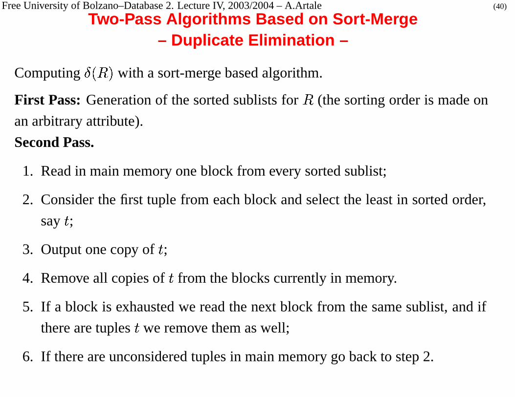
Two-Pass Algorithms Based on Sort-Merge– Duplicate Elimination –
Computing
� � � �
with a sort-merge based algorithm.
First Pass: Generation of the sorted sublists for
�
(the sorting order is made on
an arbitrary attribute).
Second Pass.
1. Read in main memory one block from every sorted sublist;
2. Consider the first tuple from each block and select the least in sorted order,
say
�
;
3. Output one copy of
�
;
4. Remove all copies of
�
from the blocks currently in memory.
5. If a block is exhausted we read the next block from the same sublist, and if
there are tuples
�
we remove them as well;
6. If there are unconsidered tuples in main memory go back to step 2.
Free University of Bolzano–Database 2. Lecture IV, 2003/2004 – A.Artale (41)
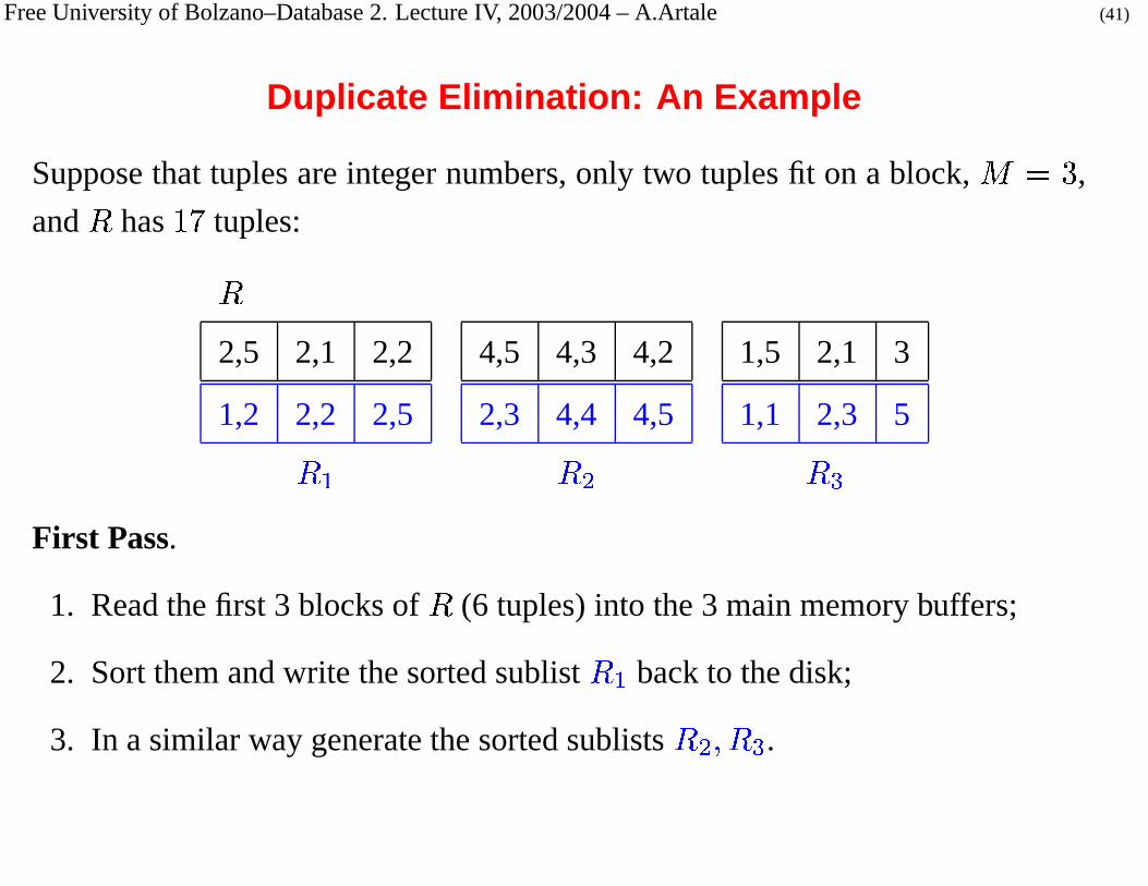
Duplicate Elimination: An Example
Suppose that tuples are integer numbers, only two tuples fit on a block,
� � �
,
and
�
has
� �
tuples:
�
2,5 2,1 2,2 4,5 4,3 4,2 1,5 2,1 3
1,2 2,2 2,5 2,3 4,4 4,5 1,1 2,3 5
� � � � ���
First Pass.
1. Read the first 3 blocks of
�
(6 tuples) into the 3 main memory buffers;
2. Sort them and write the sorted sublist
� � back to the disk;
3. In a similar way generate the sorted sublists
� � �
��� .

Free University of Bolzano–Database 2. Lecture IV, 2003/2004 – A.Artale (42)
Duplicate Elimination: An Example (cont.)
Second Pass – Cycle 1.
1. Read in main memory the first block from every sorted sublist:
Sublists Main Memory Waiting on Disk
� � ��
� ��
� ��
�
� � ��
� ��
� ��
�
��� ��
� ��
� �
2. The least tuple of the three blocks in main memory is
�
.
3. We copy
�
to the output:
Output Buffer
1
Free University of Bolzano–Database 2. Lecture IV, 2003/2004 – A.Artale (43)
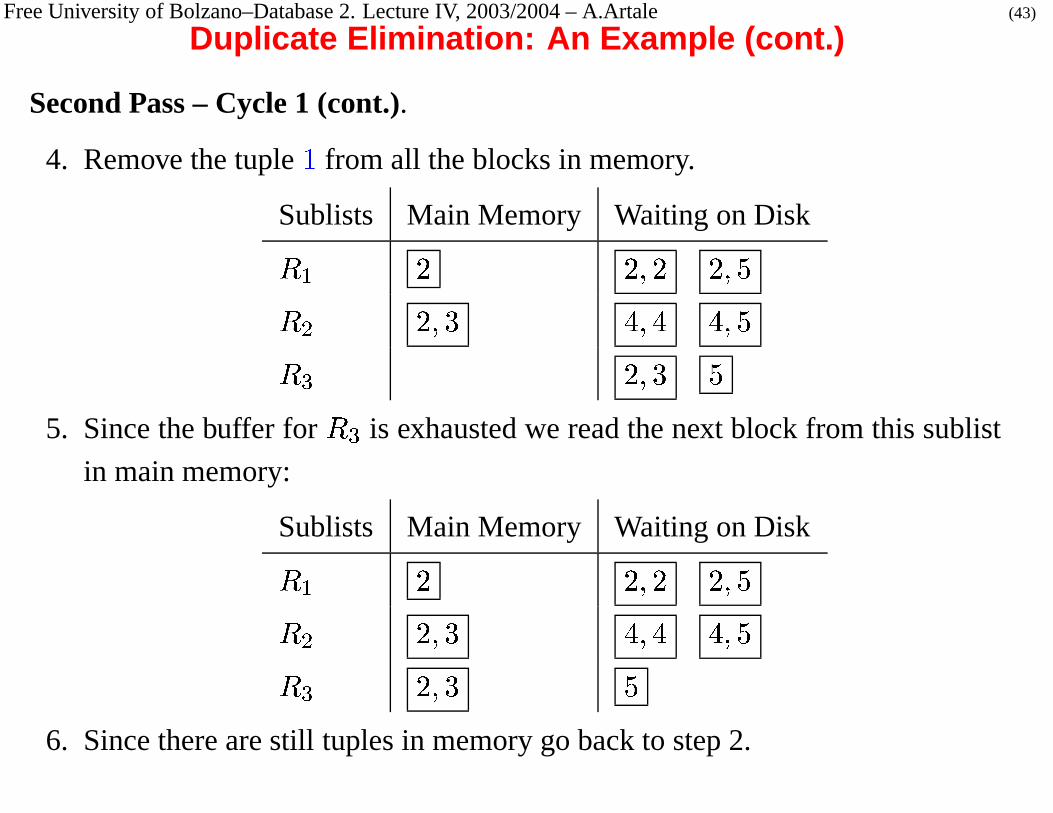
Duplicate Elimination: An Example (cont.)
Second Pass – Cycle 1 (cont.).
4. Remove the tuple
�
from all the blocks in memory.
Sublists Main Memory Waiting on Disk
� � � ��
� ��
�
� � ��
� ��
� ��
�
�� ��
� �
5. Since the buffer for
�� is exhausted we read the next block from this sublist
in main memory:
Sublists Main Memory Waiting on Disk
� � � ��
� ��
�
� � ��
� ��
� ��
�
��� ��
� �
6. Since there are still tuples in memory go back to step 2.

Free University of Bolzano–Database 2. Lecture IV, 2003/2004 – A.Artale (44)
Duplicate Elimination: An Example (cont.)
Second Pass – Cycle 2.
2. The least tuple of the three blocks in main memory is now�
.
3. We copy
�
to the output:
Output Buffer
1 2
4. Remove the tuple
�
from all the blocks in memory:
Sublists Main Memory Waiting on Disk
� � ��
� ��
�
� � � ��
� ��
�
��� � �

Free University of Bolzano–Database 2. Lecture IV, 2003/2004 – A.Artale (45)
Duplicate Elimination: An Example (cont.)
Second Pass – Cycle 2 (cont.).
5. Since the buffer for
� � is exhausted we read the next block from this sublist,
and since there are tuples
�
we remove them as well;
Sublists Main Memory Waiting on Disk
� � �
� � � ��
� ��
�
��� � �
6. Since there are still tuples in memory go back to step 2.
Free University of Bolzano–Database 2. Lecture IV, 2003/2004 – A.Artale (46)
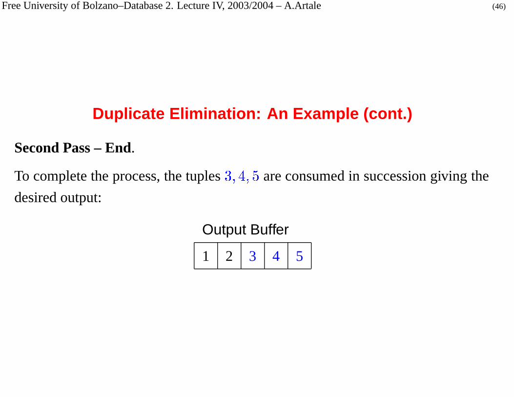
Duplicate Elimination: An Example (cont.)
Second Pass – End.
To complete the process, the tuples
��
��
�
are consumed in succession giving the
desired output:
Output Buffer
1 2 3 4 5

Free University of Bolzano–Database 2. Lecture IV, 2003/2004 – A.Artale (47)
Duplicate Elimination: Cost Analysis
� Number of Disk I/O:
� � � � � �
.
1.
� � � �
to read each block of
�
when creating the sorted sublists;
2.
� � � �
to write each sublist back to disk;
3.
� � � �
to read each block from the sublist in the second pass.
� Number of memory buffer required:
� � � � � �.
1. Assuming
�
buffers are available. Then, each sorted sublist can be at
most
�
blocks long;
2. For the second pass one block for EACH sublist should be in main
memory. Then, the number of sublists is at most
�
;
3. Given
�
available buffers, we can process at most
�
sublists, each at
most
�
blocks long:� � � � � � �
.
� Exercise. Try the example with M = 2 and verify that the algorithm goes in
Memory Overflow.

Free University of Bolzano–Database 2. Lecture IV, 2003/2004 – A.Artale (48)
Sort-Merge Natural Join
Computing
� � ��
� � � � � ��
� �
with a sort-merge based algorithm.
First Pass: Create sorted sublists for both
�
and
�
of size
�
using�
as sort key.
Second Pass.
1. Bring the first block of EACH sublist into main memory;
2. Find the tuple with the least value � for
�
;
3. If � does not appear in the blocks of the other relation then consider the
successive least �;
4. Otherwise, identify ALL the tuples from BOTH relations having sort key
�—perhaps bringing new blocks in main memory;
5. Output the joining tuples;
6. If the buffer for one of the sublists is exhausted reload the buffer for this
sublist.
7. If there are unconsidered tuples in main memory go back to step 2.

Free University of Bolzano–Database 2. Lecture IV, 2003/2004 – A.Artale (49)
Sort-Merge Natural Join: An Example
� Assume that the joining attribute is of type integer, only two tuples fit on
a block,
� � �
, and
�
and
�
both have
� �
tuples—in the following we
represent only the joining attribute.
� First Pass: generate the sorted sublists:
�
2,5 2,1 2,2 4,5 4,3 4,2 1,5 2,1 3
1,2 2,2 2,3 4,4 5,5 1,1 2,2 3,4 5
� � � �
�
2,1 2,1 1,2 2,3 3,3 3,2 6,5 4,4 4
1,1 1,2 2,2 2,3 3,3 2,3 4,4 4,5 6� � � �

Free University of Bolzano–Database 2. Lecture IV, 2003/2004 – A.Artale (50)
Sort-Merge Natural Join: An Example (Cont.)
Second Pass – Cycle 1. Note: We show the situation in main memory for each
value of the joining attribute.
� Since after Steps 1-3, 1 is the least common value for the joining attribute we
read in main memory ALL the blocks for this joining attribute (as specified
in Step 4):
Sublists Main Memory Waiting on Disk
� � ��
� ��
� ��
� ��
� ��
�
� � ��
� ��
� ��
� �
� � ��
� ��
� ��
� ��
� ��
�
� � ��
� ��
� ��
� �
Note. For the Sublist
� � two blocks are read in main memory respecting the
Step 4 of the algorithm.
� (Step 5) The Natural Join between the tuples having joining attribute = 1 is
computed and moved to the output.

Free University of Bolzano–Database 2. Lecture IV, 2003/2004 – A.Artale (51)
Sort-Merge Natural Join: An Example (Cont.)
� (Step 6) The buffer for
� � is exhausted: we read its successive block.
Sublists Main Memory Waiting on Disk
� � ��
� ��
� ��
� ��
� ��
�
� � ��
� ��
� �
� � ��
� ��
� ��
� ��
�
� � ��
� ��
� ��
� �

Free University of Bolzano–Database 2. Lecture IV, 2003/2004 – A.Artale (52)
Sort-Merge Natural Join: An Example (Cont.)
Second Pass – Cycle 2.
� (Steps 2-4) Read in main memory ALL the blocks for the joining attribute 2:
Sublists Main Memory Waiting on Disk
� � ��
� ��
� ��
� ��
� ��
�
� � ��
� ��
� �
� � ��
� ��
� ��
� ��
�
� � ��
� ��
� ��
� �
Since there are only
�
buffers available (
� � �
) while this step requires
�
buffers the algorithm fails with a memory overflow error.

Free University of Bolzano–Database 2. Lecture IV, 2003/2004 – A.Artale (53)
Sort-Merge Natural Join: Cost Analysis
� Number of Disk I/O:
� � � � � � � � � � � � �
.
1. Creating the sorted sublist costs
�
disk I/O per each block of data;
2. The merge-join phase requires reading each block of the involved
relations one more time. Thus the merge-join phase costs
� � � � � � � � � � �
disk I/O.
3. Total Cost:
� � � � � � � � � � � � �
disk I/O.
� Number of memory buffer required:� � � � � � � � � � �
.
1. This is obtained similarly to the case of sort-based duplicate elimination
noting that now
� � � � � � � � �
blocks need to be processed:� � � � � � � � � � � �.

Free University of Bolzano–Database 2. Lecture IV, 2003/2004 – A.Artale (54)
Sort-Merge Natural Join: Cost Analysis. Example
� Example. Let
� � � �� ��
� � ��
� � � �� � � ��
� � � � �, and for no � do the
tuples of
�
and
�
that agree on � occupy more than� � �
blocks. Then, the
cost of different techniques are:
Sort-Merge Join:
� � � � � � � � � � � � �� ��
� � �
disk I/O.
Sort-Based Join:
� � � � � � � � � � � � �� ��
� � �
disk I/O.
Block-Based Nested-Loop Join:� �� �
�� � � � �� � � � � � � �� ��
� � �
disk I/O.
Tuple-Based Nested-Loop Join:� � � � � � � � � � � � � �
� ��
� � ��
� � �
disk I/O.

Free University of Bolzano–Database 2. Lecture IV, 2003/2004 – A.Artale (55)
Summary
� Query Compilation and Optimization
� Algorithms for Implementing Operators
– One-Pass Algorithms
– One-And-A-Half Passes Algorithms
� Nested-Loop Join
– Two-Pass Algorithms
� Sort-Based Algorithms
� Index-Based Algorithms

Free University of Bolzano–Database 2. Lecture IV, 2003/2004 – A.Artale (56)
Index-Based Algorithms
� Index-Based Algorithms are useful for the Selection operator, but also the
other operators can take advantage.
� In the following we describe how Selection and Join operators can be
implemented taking into account the existence of indexes.

Free University of Bolzano–Database 2. Lecture IV, 2003/2004 – A.Artale (57)
Index-Based Selection
� The One-Pass algorithm scan ALL the tuples: It costs
� � � �
disk I/O.
� Suppose the query is �� � �� � �
, and there is an index on the attribute
�
.
� Algorithm: Search the index for the value � and get the pointers to
EXACTLY those tuples of
�
having value � for
�
.

Free University of Bolzano–Database 2. Lecture IV, 2003/2004 – A.Artale (58)
Index-Based Selection: Cost Analysis
� V(R,A): number of distinct values for the attribute
�
of the relation
�
.
� Number of Disk I/O
– If the index is a secondary index – tuples are spread on different blocks –
then �� � �� � �
requires about
� � � �
� � �
� ��
Disk I/O.
– If the index is a primary index – tuples with a given value are stored one
next to the other – then �� � �� � �
requires at least
� � � �
� � �
� ��
(if values are uniformly distributed).
� Note: If the index does not fit in main memory we need to consider the disk
I/O for index lookup.

Free University of Bolzano–Database 2. Lecture IV, 2003/2004 – A.Artale (59)
Index-Based Selection: An Example
The number
� � � �
� � �
� ��
is an estimate of the number of tuples with a fixed value
for the attribute
�
.
ACCOUNT
Account
�
Branch Balance
A-101 Downtown 500
A-102 Downtown 400
A-110 Downtown 600
A-201 Downtown 900
A-215 Downtown 400
A-217 Downtown 500
A-218 Downtown 900
A-222 Downtown 600
T(ACCOUNT) 8
V(ACCOUNT,Account
�
) 8
V(ACCOUNT,Branch) 1
V(ACCOUNT,Balance) 4� � � � � � �� � � �
� � � � � �� � ��
� � �� �� � � ��
1� � � � � � �� � � �
� � � � � �� � ��
� � � � � ��
8
� � � � � � �� � � �
� � � � � �� � ��
� � � � �� ��
2

Free University of Bolzano–Database 2. Lecture IV, 2003/2004 – A.Artale (60)
Selection: An Example
�� � �� � � � � � � � � �� � �� �� � � � �� ��� �� � � � �� � � � � � � � �� � � ��� �� �� �� �Suppose that
� � "! # $% &(' �� � ��
� � �
,
� � "! # $% &(' �� � � �
(i.e.,
� �
tuples per block),
) � ! # $% &('�
�+* ,- . /
-
0 ,1 ! �� � �
,
) � "! # $% &('�
243 % ' $1 ! * -
0 , 1 ! �� � � �
.
We estimate the cost of the query assuming that the following indexes exist:
1. A primary index for Branch-Name;
2. A secondary index for Customer-Name.
� Using the primary index we need to read
� �5 �6 � � 7 � �
� �5 �6 � � 7 � �� � �� � �- � � � � � � � � �
tuples,
and
� � 5 �6 � � 7 � �
� �5 �6 � � 7 � �� � �� � �- � � � � � �
89 989 � � �
blocks.
� Using the secondary index we need to read
� �5 �6 � � 7 � �
� �5 �6 � � 7 � ��� �� � � � �- � � � � � � � �
tuples. But since tuples are not stored in sequence, the number of blocks
needed is at most
� �
.
� ONE-PASS ALGORITHM takes
� � "! # $% &(' �� � � �
disk I/O.

Free University of Bolzano–Database 2. Lecture IV, 2003/2004 – A.Artale (61)
Selection: An Example (cont.)
� Intersecting pointers from both indexes in main memory:
� � � � � .
� One tuple in:
) � ! # $% &('�
� * , - . /
-
0 ,1 ! � � ) � "! # $% &('�
243 % ' $1 ! * -
0 ,1 ! �� � � � � � � � � ��
� � �
has both Branch-Name = Stretford and Customer-Name = John. Then,
� � � � � � �
, and we need to access just
�
block.
Summing up.
1. No Index:
� � �
disk I/O;
2. Primary Index:
� �
disk I/O;
3. Secondary Index:
� �
disk I/O;
4. Intersecting Pointers:
�
disk I/O;
5. Index with Concatenated Keys:
�
disk I/O.
What if there is a Disjunctive Selection?

Free University of Bolzano–Database 2. Lecture IV, 2003/2004 – A.Artale (62)
Index-Based Join
Computing
� � ��
� � � � � ��
� �
assuming that
�
has an index for
�
:
1. Read each block of
�
and for each tuple �, with �� its projection on the
�
attributes:
(a) Use the index on
�
with search key �� to find all the tuples of
�
that can
be joined with �;
(b) Output the joining tuples.
Note: This procedure is essentially a nested loop algorithm that just takes
advantage from the existence of an index to selectively search
�
.

Free University of Bolzano–Database 2. Lecture IV, 2003/2004 – A.Artale (63)
Index-Based Join: Cost Analysis
Cost Analysis
� Reading the full
�
costs
� � � �
disk I/O.
� For each tuple of
�
we must read about
� �� �� ��
�� � tuples of
�
, then we need to
distinguish two cases:
1.
�
has a secondary index for
�
then reading
�
costs
� � � � �� � �� �
� ���
� ��
� Total Number of disk I/O:
� � � � � � � � � �� � �� �
� ���
� ��
;
2.
�
has a primary index for�
then reading
�
costs
� � � � �� � �� �
� ���
� ��
� Total Number of disk I/O:
� � � � � � � � � �� � �� �
� ���
� ��
.
Free University of Bolzano–Database 2. Lecture IV, 2003/2004 – A.Artale (64)
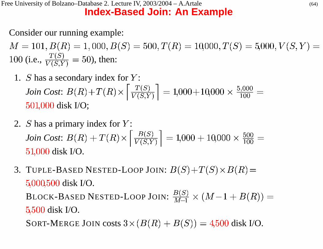
Index-Based Join: An Example
Consider our running example:� � � � ��
� � � �� ��
� � ��
� � � �� � � ��
� � � �� � ��
� � ��
� � � �� ��
� � ��
) � ��
� ��
� � �
(i.e.,
� �� �� ��
�� � � � �
), then:
1.
�
has a secondary index for
�
:
Join Cost:
� � � � � � � � � �� � �� �
� ���
� ��
� ��
� � � � � ��
� � � � 8�
9 9 9� 9 9 �
� � ��
� � �
disk I/O;
2.
�
has a primary index for
�
:
Join Cost:
� � � � � � � � � �� � �� �
� ���
� ��
� ��
� � � � � ��
� � � � 89 9� 9 9 �
� ��
� � �
disk I/O.
3. TUPLE-BASED NESTED-LOOP JOIN:
� � � � � � � � � � � � � ��
��
� � ��
� � �
disk I/O.
BLOCK-BASED NESTED-LOOP JOIN:
� �� ��� � � � �� � � � � � � �
�
��
� � �
disk I/O.
SORT-MERGE JOIN costs
� � � � � � � � � � � � �� ��
� � �
disk I/O.

Free University of Bolzano–Database 2. Lecture IV, 2003/2004 – A.Artale (65)
Index-Based Join: An Example (cont.)
A better situation if there is an index on the bigger relation:
�
�
has a primary index for
�
, and
� � �
� � �
� � � � �
(i.e.,
) � ��
� �� � � �
):
Join Cost =
� � � � � � � � � �� � � �
� ��
� ��
� � � � � ��
� � � � ��
9 9 9�9 9 �
� ��
� � �
disk I/O.
� If
�
is also a key, i.e.,
� � �
� ��
� � � �(i.e.,
) � ��
� �� � ��
� � �
):
Join Cost =
� � � � � � � � � � � � � � � � ��
� � � � ��
� � �
disk I/O.

Free University of Bolzano–Database 2. Lecture IV, 2003/2004 – A.Artale (66)
Summary of Join Algorithms Performances
� Sort-Based Join algorithms are in general the most efficient algorithms to
compute a Join;
� Block-Based Nested-Loop Join algorithms are used when there are many
tuples sharing a common attribute (sort-based join could stop because of a
memory overflow);
� Index-Based Join algorithms are comparable with sort-based join when the
biggest relation has a primary index on the joining attribute.

Free University of Bolzano–Database 2. Lecture IV, 2003/2004 – A.Artale (67)
Summary of Lecture IV
� Query Compilation and Optimization
� Algorithms for Implementing Operators
– One-Pass Algorithms
– One-And-A-Half Passes Algorithms
� Nested-Loop Join
– Two-Pass Algorithms
� Sort-Based Algorithms
� Index-Based Algorithms


![Extracting Multiple Viewpoint Models from Relational Databases · Extracting Multiple Viewpoint Models from Relational Databases Alessandro Berti1[0000 0003 1830 4013] and Wil van](https://img.pdfslide.us/doc/110x75/5fc501cddd902a49e30646ac/extracting-multiple-viewpoint-models-from-relational-extracting-multiple-viewpoint.jpg)