Database Management Systems, R. Ramakrishnan and J. Gehrke1 Evaluation of Relational Operations Chapter 12, Part A

Database Management Systems, R. Ramakrishnan and J. Gehrke 1

Evaluation of Relational Operations

Chapter 12, Part A


Relational Operations We will consider how to implement:

– Selection ( ) Selects a subset of rows from relation.– Projection ( ) Deletes unwanted columns from

relation.– Join ( ) Allows us to combine two relations.– Set-difference ( ) Tuples in reln. 1, but not in reln. 2.– Union ( ) Tuples in reln. 1 and in reln. 2.– Aggregation (SUM, MIN, etc.) and GROUP BY

Since each op returns a relation, ops can be composed! After we cover the operations, we will discuss how to optimize queries formed by composing them.


Schema for Examples

Similar to old schema; rname added for variations.

Reserves:– Each tuple is 40 bytes long, 100 tuples per page,

1000 pages. Sailors:

– Each tuple is 50 bytes long, 80 tuples per page, 500 pages.

Sailors (sid: integer, sname: string, rating: integer, age: real)Reserves (sid: integer, bid: integer, day: dates, rname: string)


Equality Joins With One Join Column

In algebra: R S. Common! Must be carefully optimized. R S is large; so, R S followed by a selection is inefficient.

Assume: M tuples in R, pR tuples per page, N tuples in S, pS tuples per page.– In our examples, R is Reserves and S is Sailors.

We will consider more complex join conditions later. Cost metric: # of I/Os. We will ignore output costs.

SELECT *FROM Reserves R1, Sailors S1WHERE R1.sid=S1.sid


Simple Nested Loops Join

For each tuple in the outer relation R, we scan the entire inner relation S. – Cost: M + pR * M * N = 1000 + 100*1000*500 I/Os.

Page-oriented Nested Loops join: For each page of R, get each page of S, and write out matching pairs of tuples <r, s>, where r is in R-page and S is in S-page.– Cost: M + M*N = 1000 + 1000*500– If smaller relation (S) is outer, cost = 500 + 500*1000

foreach tuple r in R doforeach tuple s in S do

if ri == sj then add <r, s> to result


Index Nested Loops Join

If there is an index on the join column of one relation (say S), can make it the inner and exploit the index.– Cost: M + ( (M*pR) * cost of finding matching S tuples)

For each R tuple, cost of probing S index is about 1.2 for hash index, 2-4 for B+ tree. Cost of then finding S tuples (assuming Alt. (2) or (3) for data entries) depends on clustering.– Clustered index: 1 I/O (typical), unclustered: upto 1 I/O

per matching S tuple.

foreach tuple r in R doforeach tuple s in S where ri == sj do

add <r, s> to result


Examples of Index Nested Loops

Hash-index (Alt. 2) on sid of Sailors (as inner):– Scan Reserves: 1000 page I/Os, 100*1000 tuples.– For each Reserves tuple: 1.2 I/Os to get data entry in

index, plus 1 I/O to get (the exactly one) matching Sailors tuple. Total: 220,000 I/Os.

Hash-index (Alt. 2) on sid of Reserves (as inner):– Scan Sailors: 500 page I/Os, 80*500 tuples.– For each Sailors tuple: 1.2 I/Os to find index page with

data entries, plus cost of retrieving matching Reserves tuples. Assuming uniform distribution, 2.5 reservations per sailor (100,000 / 40,000). Cost of retrieving them is 1 or 2.5 I/Os depending on whether the index is clustered.


Block Nested Loops Join Use one page as an input buffer for scanning the

inner S, one page as the output buffer, and use all remaining pages to hold ``block’’ of outer R.– For each matching tuple r in R-block, s in S-page, add

<r, s> to result. Then read next R-block, scan S, etc.

. . .

. . .

R & SHash table for block of R

(k < B-1 pages)

Input buffer for S Output buffer

. . .

Join Result


Examples of Block Nested Loops

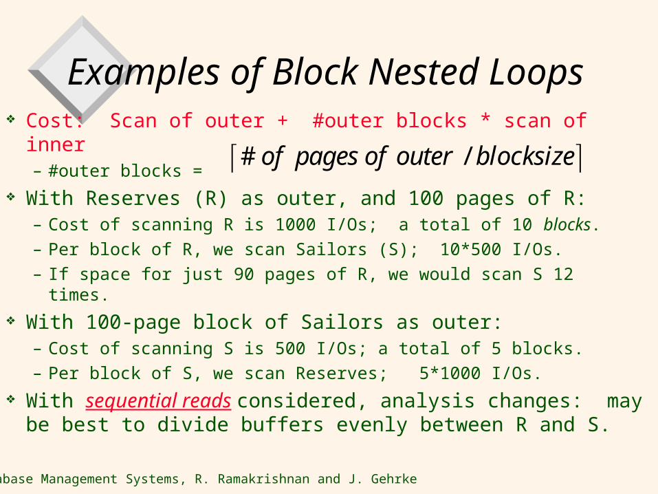
Cost: Scan of outer + #outer blocks * scan of inner– #outer blocks =

With Reserves (R) as outer, and 100 pages of R:– Cost of scanning R is 1000 I/Os; a total of 10 blocks.– Per block of R, we scan Sailors (S); 10*500 I/Os.– If space for just 90 pages of R, we would scan S 12 times.

With 100-page block of Sailors as outer:– Cost of scanning S is 500 I/Os; a total of 5 blocks.– Per block of S, we scan Reserves; 5*1000 I/Os.

With sequential reads considered, analysis changes: may be best to divide buffers evenly between R and S.

# /of pages of outer blocksize


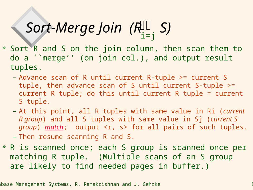
Sort-Merge Join (R S) Sort R and S on the join column, then scan them to do

a ``merge’’ (on join col.), and output result tuples.– Advance scan of R until current R-tuple >= current S tuple,

then advance scan of S until current S-tuple >= current R tuple; do this until current R tuple = current S tuple.

– At this point, all R tuples with same value in Ri (current R group) and all S tuples with same value in Sj (current S group) match; output <r, s> for all pairs of such tuples.

– Then resume scanning R and S. R is scanned once; each S group is scanned once per

matching R tuple. (Multiple scans of an S group are likely to find needed pages in buffer.)

i=j


Example of Sort-Merge Join

Cost: M log M + N log N + (M+N)– The cost of scanning, M+N, could be M*N (very unlikely!)

With 35, 100 or 300 buffer pages, both Reserves and Sailors can be sorted in 2 passes; total join cost: 7500.

sid sname rating age22 dustin 7 45.028 yuppy 9 35.031 lubber 8 55.544 guppy 5 35.058 rusty 10 35.0

sid bid day rname

28 103 12/4/96 guppy28 103 11/3/96 yuppy31 101 10/10/96 dustin31 102 10/12/96 lubber31 101 10/11/96 lubber58 103 11/12/96 dustin

(BNL cost: 2500 to 15000 I/Os)


Refinement of Sort-Merge Join

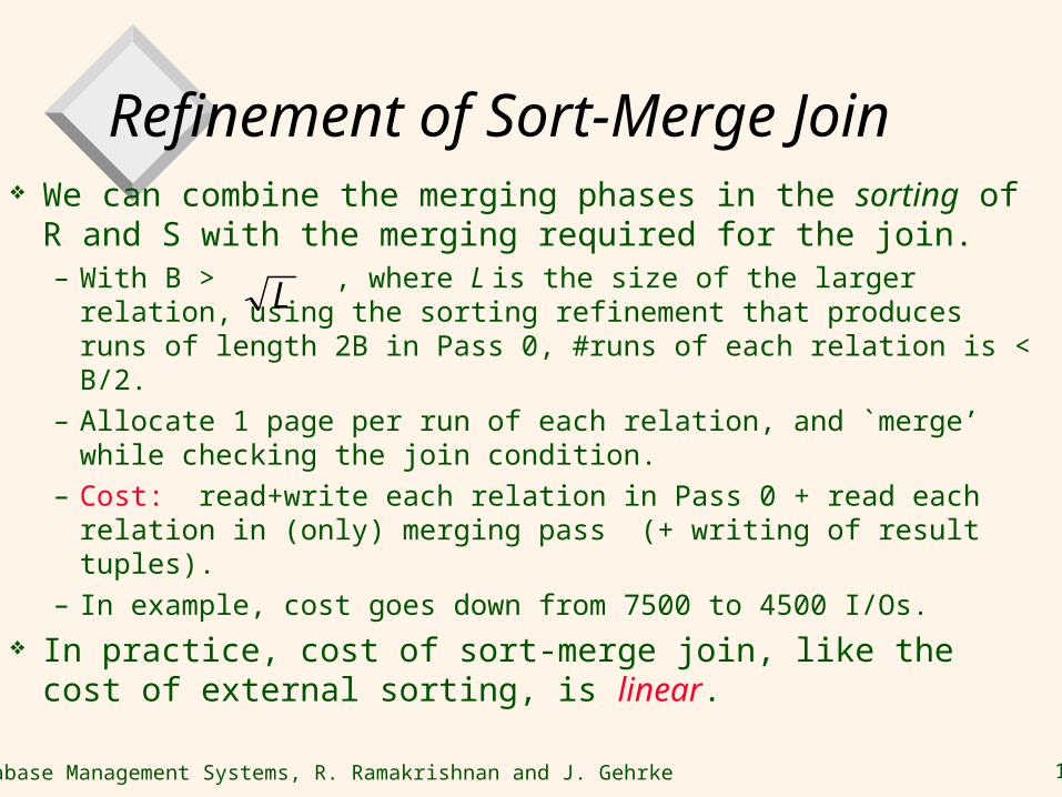
We can combine the merging phases in the sorting of R and S with the merging required for the join.– With B > , where L is the size of the larger relation,

using the sorting refinement that produces runs of length 2B in Pass 0, #runs of each relation is < B/2.

– Allocate 1 page per run of each relation, and `merge’ while checking the join condition.

– Cost: read+write each relation in Pass 0 + read each relation in (only) merging pass (+ writing of result tuples).

– In example, cost goes down from 7500 to 4500 I/Os. In practice, cost of sort-merge join, like the cost of

external sorting, is linear.

L


Hash-Join Partition both

relations using hash fn h: R tuples in partition i will only match S tuples in partition i.

Read in a partition of R, hash it using h2 (<> h!). Scan matching partition of S, search for matches.

Partitionsof R & S

Input bufferfor Si

Hash table for partitionRi (k < B-1 pages)

B main memory buffersDisk

Output buffer

Disk

Join Result

hashfnh2

h2

B main memory buffers DiskDisk

Original Relation OUTPUT

2INPUT

1

hashfunction

h B-1

Partitions

1

2

B-1

. . .


Observations on Hash-Join

#partitions k < B-1 (why?), and B-2 > size of largest partition to be held in memory. Assuming uniformly sized partitions, and maximizing k, we get:– k= B-1, and M/(B-1) < B-2, i.e., B must be >

If we build an in-memory hash table to speed up the matching of tuples, a little more memory is needed.

If the hash function does not partition uniformly, one or more R partitions may not fit in memory. Can apply hash-join technique recursively to do the join of this R-partition with corresponding S-partition.

M


Cost of Hash-Join

In partitioning phase, read+write both relns; 2(M+N). In matching phase, read both relns; M+N I/Os.

In our running example, this is a total of 4500 I/Os. Sort-Merge Join vs. Hash Join:

– Given a minimum amount of memory (what is this, for each?) both have a cost of 3(M+N) I/Os. Hash Join superior on this count if relation sizes differ greatly. Also, Hash Join shown to be highly parallelizable.

– Sort-Merge less sensitive to data skew; result is sorted.


General Join Conditions Equalities over several attributes (e.g., R.sid=S.sid

AND R.rname=S.sname):– For Index NL, build index on <sid, sname> (if S is inner);

or use existing indexes on sid or sname.– For Sort-Merge and Hash Join, sort/partition on

combination of the two join columns. Inequality conditions (e.g., R.rname < S.sname):

– For Index NL, need (clustered!) B+ tree index. Range probes on inner; # matches likely to be much higher than

for equality joins.

– Hash Join, Sort Merge Join not applicable.– Block NL quite likely to be the best join method here.

Documents

Database Management Systems, R. Ramakrishnan and J. Gehrke1 Evaluation of Relational Operations Chapter 12, Part A