Embed Size (px)
Citation preview

Database design with UML and SQL, 3rd
edition
Welcome to students in Dr. Klusener's class at Vreije Universitiet Amsterdam! And many
thanks to readers who have found this site useful. Yes, I'm still considering how to make
exercise answers available, and possibly how to produce an easily-printable version. Watch
for updates here!
Also available on tomjewett.com: web accessibility resources and consulting.
Introduction
This third edition of dbDesign is a general update, both to meet legal requirements for U.S.
“Section 508” accessibility and to bring the code into compliance with the latest World Wide
Web Consortium standards. In the process, I've tried to make the SQL examples as generic as
possible, although you will still have to consult the documentation for your own database
system. Graphics no longer require the SVG plugin; large-image and text-only views of each
graphic are provided for all readers; the menu is now arranged by topic areas; and the print
version (minus left-side navigation) is done automatically by a style sheet.
The second edition was largely motivated by the very helpful comments of Prof. Alvaro
Monge, as well as by my own observations in two semesters of using its predecessor in class.
Major changes included the clear separation of UML from its implementation in the
relational model, the introduction of relational algebra terminology as an aid to understanding
SQL, and an increased emphasis on natural-language understanding of the design.
The original site was the outgrowth of a previous book project, Practical Relational
Database Design, by Wayne Dick and Tom Jewett. The move online featured condensed
discussions, an integrated view of database concepts and skills, and use of the Unified
Modeling Language in the design process. I’m grateful for the positive response that the site
has received so far, both from my own students and from online readers worldwide.
In every edition of this site, I owe a huge debt of gratitude to Prof. Wayne Dick, lead author
of the earlier PRDD book and internationally-known accessibility expert. We’ve worked
together for so long that it’s hard to identify separate authorship of the material here—I hope
that this general acknowledgement will suffice. The students in my Fall 2002 class were
especially helpful in “test driving” each page and asking lots of questions! As always with
teaching materials, my students are the main source of inspiration and motivation to develop
the site.
Tom Jewett Department of Computer Engineering and Computer Science, Emeritus
California State University, Long Beach
www.cecs.csulb.edu/~jewett/
email: [email protected]
Copyright © 2002–2006, by Tom Jewett. Links to this site are welcome and encouraged.
Individual copies may be printed for non-commercial classroom or personal use; however,
this material may not be reposted to other web sites or newsgroups, or included in any printed
or electronic publication, whether modified or not, without specific permission from the
author.
Database design is a process of modeling an enterprise in the real world. In fact, a database
itself is a model of the real world that contains selected information needed by the enterprise.
Many models and languages—some formally and mathematically defined, some informal and
intuitive—are used by designers. Here are the ones that we present in this tutorial:
• The Unified Modeling Language (UML) was designed for software engineering of large
systems using object-oriented (OO) programming languages. UML is a very large language;
we will use only a small portion of it here, to model those portions of an enterprise that will
be represented in the database. It is our tool for communicating with the client in terms that
are used in the enterprise.
• The Entity-Relationship (ER) model is used in many database development systems. There
are many different graphic standards that can represent the ER model. Some of the most
modern of these look very similar to the UML class diagram, but may also include elements
of the relational model.
• The Relational Model (RM) is the formal model of a database that was developed for IBM
in the early 1970s by Dr. E.F. Codd. It is largely based on set theory, which makes it both
powerful and easy to implement in computers. All modern relational databases are based on
this model. We will use it to represent information that does not (and should not) appear in
the UML model but is needed for us to build functioning databases.
• Relational Algebra (RA) is a formal language used to symbolically manipulate objects of
the relational model.
• The table model is an informal set of terms for relational model objects. These are the
terms used most often by database developers.
• The Structured Query Language (SQL, pronounced “sequel” or “ess-que-ell”) is used to
build and manipulate relational databases. It is based on relational algebra, but provides
additional capabilities that are needed in commercial systems. It is a declarative, rather than a
procedural, programming language. There is a standard for this language, but products vary
in how closely they implement it.
Basic structures: classes and schemes
The UML class
A UML class (ER term: entity) is any “thing” in the enterprise that is to be represented in our
database. It could be a physical “thing” or simply a fact about the enterprise or an event that
happens in the real world.
Example: We’ll build a sales database—it could be for any kind of business. To sell anything,
we need customers, so a Customer will be our first class (entity) type.
• The first step in modeling a class is to describe it in natural language. This helps us to know
exactly what this class (“thing”) means in the enterprise. We can describe a customer like
this:
“A customer is any person who has done business with us or who we think might do business
with us in the future. We need to know this person’s name, phone number and address in
order to contact him or her.”
• Each class is uniquely defined by its set of attributes (UML and ER), also called properties
in some OO languages. Each attribute is one piece of information that characterizes each
member of this class in the database. Together, they provide the structure for our database
tables or code objects.
• In UML, we will only identify descriptive attributes—those which actually provide real-
world information (relevant to the enterprise) about the class that we are modeling. (These
are sometimes called natural attributes.) We will not add “ID numbers” or similar attributes
that we make up to use only inside the database.
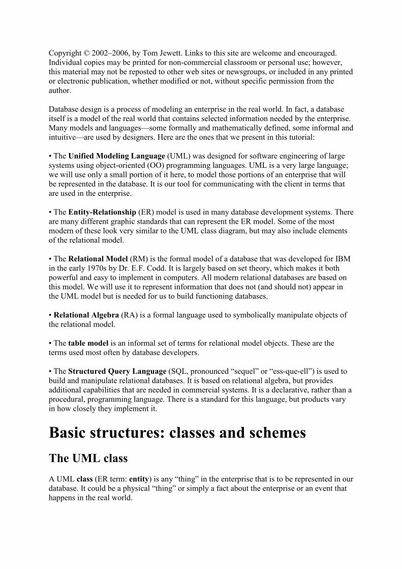
Class diagram
The class diagram shows the class name (always a singular noun) and its list of attributes.
Other views of this diagram: Large image - Data dictionary (text)
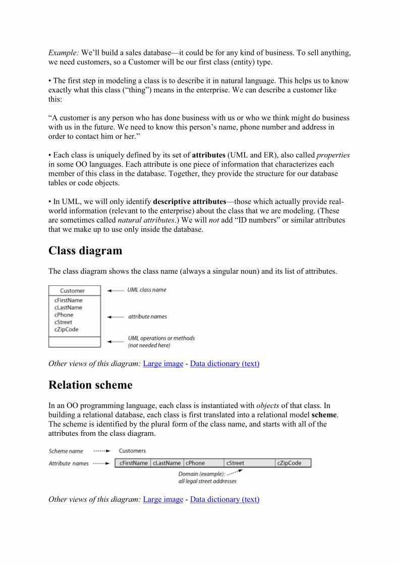
Relation scheme
In an OO programming language, each class is instantiated with objects of that class. In
building a relational database, each class is first translated into a relational model scheme.
The scheme is identified by the plural form of the class name, and starts with all of the
attributes from the class diagram.
Other views of this diagram: Large image - Data dictionary (text)
• In the relational model, a scheme is defined as a set of attributes, together with an
assignment rule that associates each attribute with a set of legal values that may be assigned
to it. These values are called the domain of the attribute. We’ve chosen to show the scheme
graphically, but we could also have written it in set notation:
Customers Scheme = {cFirstname, cLastname, cPhone, cStreet, cZipCode}.
• There is no convenient graphical way to represent domains; we’ll discuss this issue in a
later page. For the moment, our Customers relation scheme looks exactly like the Customer
class diagram, only drawn sideways. It won’t stay that way for long.
• It’s important to recognize that defining schemes or domains as sets of something
automatically tells us a lot more about them:
- They cannot contain duplicate elements. Our Customers scheme, for example, cannot have
two cPhone attributes (even if they are called cPhone1 and cPhone2).
- The elements in them are unordered. It doesn't matter if a customer's name is listed in order
“Last, First” or “First Last”—they mean the same thing.
- We can develop rules for what can be included in them and what is excluded from them.
For example, zip codes don’t belong in the domain (set) of phone numbers, and vice-versa.
- We can define subsets of them—for example, we can display only a selected set of
attributes from a scheme, or we can limit the domain of an attribute to a specific range of
values.
- They may be manipulated with the usual set operators. In a later page, we will show how
both the union and the intersection of schemes are used to join (combine) the information
from two or more tables based on different schemes.
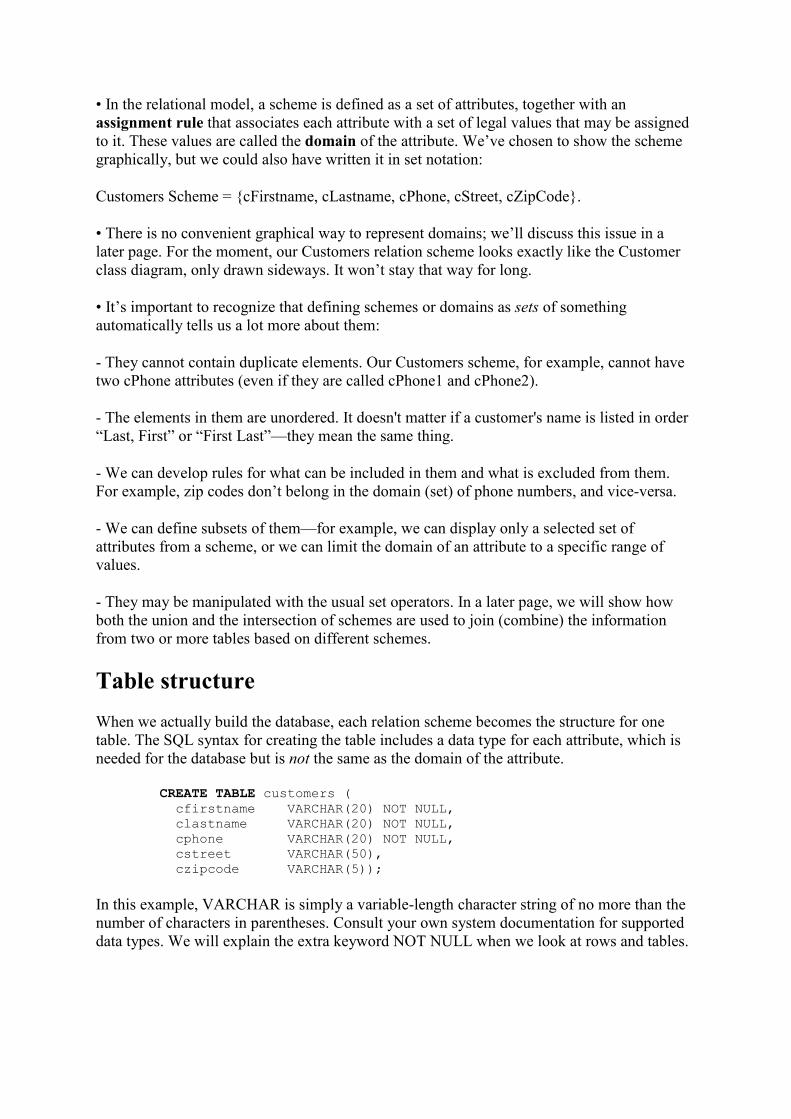
Table structure
When we actually build the database, each relation scheme becomes the structure for one
table. The SQL syntax for creating the table includes a data type for each attribute, which is
needed for the database but is not the same as the domain of the attribute.
CREATE TABLE customers (
cfirstname VARCHAR(20) NOT NULL,
clastname VARCHAR(20) NOT NULL,
cphone VARCHAR(20) NOT NULL,
cstreet VARCHAR(50),
czipcode VARCHAR(5));
In this example, VARCHAR is simply a variable-length character string of no more than the
number of characters in parentheses. Consult your own system documentation for supported
data types. We will explain the extra keyword NOT NULL when we look at rows and tables.

Exercise: designing classes
Design classes to represent the following “things” in the given enterprises. For each one,
describe the class in English, then draw the class diagram.
• A student at a university.
• A faculty member at a university.
• A work of art that is displayed in a gallery or museum.
• An automobile that is registered with the Motor Vehicle Department.
• A pizza that is on the menu at a restaurant.
The solution to this exercise will be discussed in class or posted online at a later date.
Basic structures: rows and tables
Representing data in rows
Each real-world individual of a class (for example, each customer who does business with
our enterprise) is represented by a row of information in a database table. The row is defined
in the relational model as a tuple that is constructed over a given scheme. Mathematically,
the tuple is a function that assigns a constant value from the attribute domain to each attribute
of the scheme. Notice that because the scheme is a set of attributes, we could show them in
any order without changing the meaning of the data in the row (tuple).
Other views of this diagram: Large image - Description (text)
In formal notation, we could show the assignments explicitly, where t represents a tuple:
tTJ = ‹cfirstname := 'Tom', clastname := 'Jewett', cphone := '714-555-1212', cstreet := '10200
Slater', czipcode := '92708'›
In practice, when we create a table row in SQL, we are actually making the assignment of
domain values to attributes, just as in the tuple definition.
INSERT INTO customers
(cfirstname, clastname, cphone, cstreet, czipcode)
VALUES ('Tom', 'Jewett', '714-555-1212', '10200 Slater',
'92708');

In SQL, you can omit the attribute names from the INSERT INTO statement, as long as you
keep the comma-delimited list of values in exactly the same order that was used to create the
table.
When we change the data in a table row using SQL, we are also following the tuple definition
of assigning domain values to attributes.
UPDATE customers
SET cphone = '714-555-2323'
WHERE cphone = '714-555-1212';
Tables
A database table is simply a collection of zero or more rows. This follows from the relational
model definition of a relation as a set of tuples over the same scheme. (The name “relational
model” comes from the relation being the central object in this model.)
Other views of this diagram: Large image - Description (text)
• Knowing that the relation (table) is a set of tuples (rows) tells us more about this structure,
as we saw with schemes and domains.
- Each tuple/row is unique; there are no duplicates
- Tuples/rows are unordered; we can display them in any way we like and the meaning
doesn’t change. (SQL gives us the capability to control the display order.)
- Tuples/rows may be included in a relation/table set if they are constructed on the scheme of
that relation; they are excluded otherwise. (It would make no sense to have an Order row in
the Customers table.)
- We can define subsets of the rows by specifying criteria for inclusion in the subset. (Again,
this is part of a SQL query.)
- We can find the union, intersection, or difference of the rows in two or more tables, as long
as they are constructed over the same scheme.
Insuring unique rows
Since each row in a table must be unique, no two rows can have exactly the same values for
every one of their attributes. Therefore, there must be some set of attributes (it might be the
set of all attributes) in each relation whose values, taken together, guarantee uniqueness of
each row. Any set of attributes that can do this is called a super key (SK). Super keys are a
property of the relation (table), filled in with any reasonable set of real-world data, even
though we show them in the relation scheme drawing for convenience.
The database designer picks one of the possible super key attribute sets to serve as the
primary key (PK) of the relation. (Notice that the PK is an SK, but not all SKs are PKs!) The
PK is sometimes also called a unique identifier for each row of the table. This is not an
arbitrary choice—we’ll discuss it in detail on a later page. For our customers table, we’ll pick
the customer’s first name, last name, and phone number. We are likely to have at least two
customers with the same first and last name, but it is very unlikely that they will both have
the same phone number.
In SQL, we specify the primary key with a constraint on the table that lists the PK attributes.
We also give the constraint a name that is easy for us to remember later (like “customers_pk”
here).
ALTER TABLE customers
ADD CONSTRAINT customers_pk
PRIMARY KEY (cfirstname, clastname, cphone);
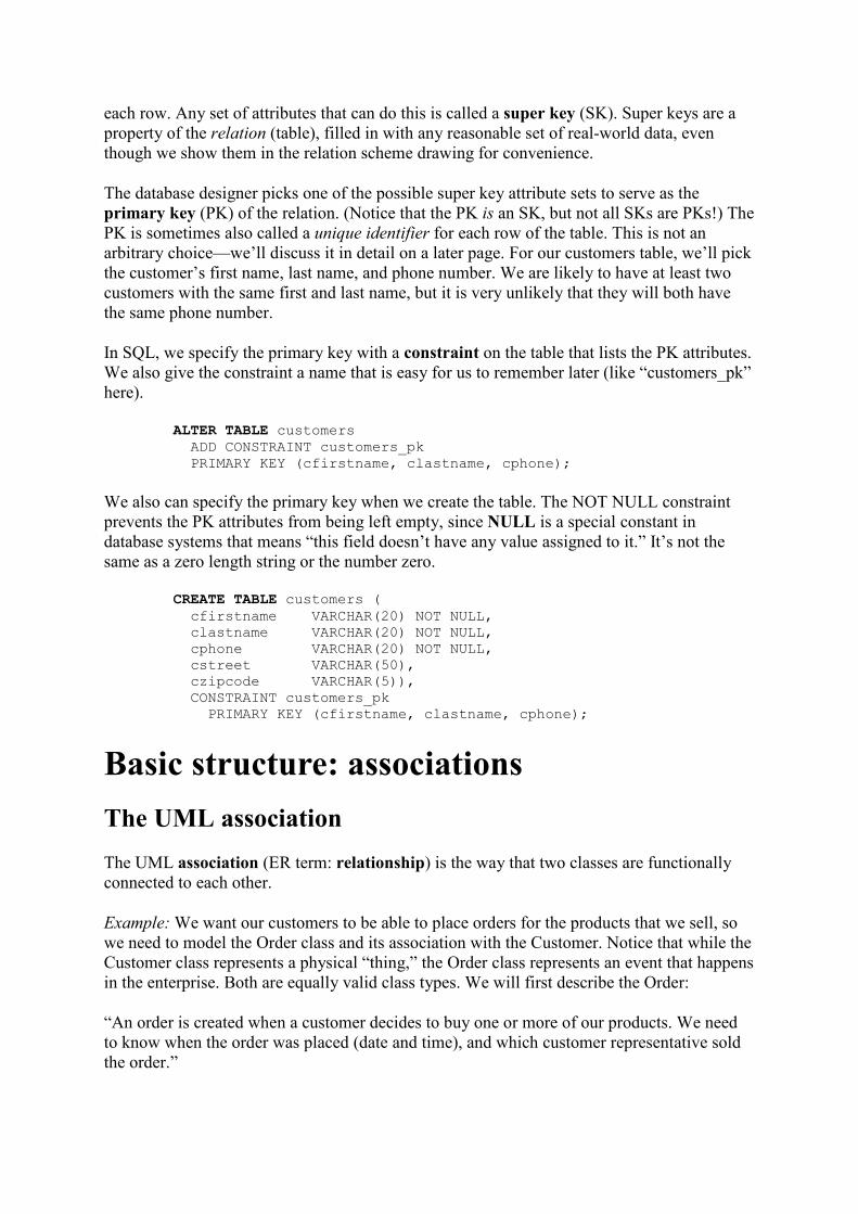
We also can specify the primary key when we create the table. The NOT NULL constraint
prevents the PK attributes from being left empty, since ,ULL is a special constant in
database systems that means “this field doesn’t have any value assigned to it.” It’s not the
same as a zero length string or the number zero.
CREATE TABLE customers (
cfirstname VARCHAR(20) NOT NULL,
clastname VARCHAR(20) NOT NULL,
cphone VARCHAR(20) NOT NULL,
cstreet VARCHAR(50),
czipcode VARCHAR(5)),
CONSTRAINT customers_pk
PRIMARY KEY (cfirstname, clastname, cphone);
Basic structure: associations
The UML association
The UML association (ER term: relationship) is the way that two classes are functionally
connected to each other.
Example: We want our customers to be able to place orders for the products that we sell, so
we need to model the Order class and its association with the Customer. Notice that while the
Customer class represents a physical “thing,” the Order class represents an event that happens
in the enterprise. Both are equally valid class types. We will first describe the Order:
“An order is created when a customer decides to buy one or more of our products. We need
to know when the order was placed (date and time), and which customer representative sold
the order.”

The association between the customer and the order will tell us which customer placed the
order. We will describe the association in natural language just as we described the classes,
but we will also include information about how few (at minimum) and how many (at
maximum) individuals of one class may be connected to a single individual of the other class.
This is called the multiplicity of the association (ER term: cardinality), and we describe it in
both directions.
“Each customer places zero or more orders.” (* in the diagram below means “many”, and any
quantity more than one is the same as “many” in a database.)
“Each order is placed by one and only one customer.” (Bad English—passive voice—but
makes sense!)
Class diagram
Other views of this diagram: Large image - Data dictionary (text)
• In the diagram, the association is simply shown by a line connecting the two class types. It
is named with a verb that describes the action; an arrow shows which way to read the verb.
Symbols at each end of the line represent the multiplicity of the association, as we described
it above.
• Looking at the maximum multiplicity at each end of the line (1 and * here), we call this a
one-to-many association.
• The UML representation of the Order class contains only its own descriptive attributes. The
UML association tells which customer placed an order. In the database, we will need a
different way to identify the customer; that will be part of the relation scheme (below).
Relation scheme diagram
The relation scheme for the new Orders table contains all of the attributes from the class
diagram, as before. But we also need to represent the association in the database; that is, we
need to record which customer placed each order. We do this by copying the PK attributes of
the Customer into the Orders scheme. The copied attributes are called a foreign key (FK),
which is simply an image of the linked relation’s primary key.

Other views of this diagram: Large image - Data dictionary (text)
• Since we can’t have an order without a customer, we call Customers the parent and Orders
the child scheme in this association. The “one” side of an association is always the parent,
and provides the PK attributes to be copied. The “many” side of an association is always the
child, into which the FK attributes are copied. Memorize it: one, parent, PK; many, child, FK.
• An FK might or might not become part of the PK of the child relation into which it is
copied. In this case, it does, since we need to know both who placed an order and when the
order was placed in order to identify it uniquely.
The child table
The Orders table is created in exactly the same way as the Customers, including all of the
attributes from the Orders scheme:
CREATE TABLE orders (
cfirstname VARCHAR(20),
clastname VARCHAR(20),
cphone VARCHAR(20),
orderdate DATE,
soldby VARCHAR(20));
• Notice that the FK attributes must be exactly the same data type and size as they were
defined in the PK table.
• The DATE data type includes the time in some database systems, but not in others (which
would need an additional ordertime attribute to permit more than one order per customer in a
single day). For simplicity, we have omitted the time from our illustrations.
• To insure that every row of the Orders table is unique, we need to know both who the
customer is and what day (and time) the order was placed. We specify all of these attributes
as the pk:
ALTER TABLE orders
ADD CONSTRAINT orders_pk
PRIMARY KEY (cfirstname, clastname, cphone, orderdate);
• In addition, we need to identify which attributes make up the FK, and where they are found
as a PK. The FK constraint will insure that every order contains a valid customer name and
phone number—this is called maintaining the referential integrity of the database.

ALTER TABLE orders
ADD CONSTRAINT orders_customers_fk
FOREIGN KEY (cfirstname, clastname, cphone)
REFERENCES customers (cfirstname, clastname, cphone);
• When you look at some typical data in the Orders table, you will see that some customers
have placed more than one order. For each of these, the same customer information is copied
in the FK columns—but the dates will be different. Of course, we hope to see many orders
that were placed on the same date—but the customers will be different. You will also see that
some customers haven’t placed any orders at all; their PK information is simply not found in
the orders table.
Orders
cfirstname clastname cphone orderdate soldby
Alvaro Monge 562-333-4141 2003-07-14 Patrick
Wayne Dick 562-777-3030 2003-07-14 Patrick
Alvaro Monge 562-333-4141 2003-07-18 Kathleen
Alvaro Monge 562-333-4141 2003-07-20 Kathleen
.ote: The date format shown in our examples ('yyyy-mm-dd') is used by many but not all
systems. Consult the reference for your own software to be sure.
Exercise: patients and blood samples
(Wayne Dick)
The one-to-many association is perhaps the most common one that you will encounter in
database modeling. As an example, we will look at the enterprise of a medical clinic.
We wish to track the level of various substances (for example, cholesterol or alcohol) in the
blood of patients. For each blood sample that is taken from the patient, one test will be
performed and the date of the sample, the substance tested, and the measured level of that
substance will be recorded in a database.
• Describe each class in English.
• Draw the class diagram.
• Describe each association in English (both directions).
• Draw the relation scheme.
The solution to this exercise will be discussed in class or posted online at a later date.
Exercise: cities and states
Part of a database that you are developing will contain information about cities and states in
the United States. Each city is located in only one state. (Texarkana, Texas is a different city
than Texarkana, Arkansas.)
• Describe each class in English.
• Draw the class diagram.
• Describe each association in English (both directions).
• Draw the relation scheme.
The solution to this exercise will be discussed in class or posted online at a later date.
Exercise: library books
You are building a very simplified beginning of the database for a library. The library, of
course, owns (physical) books that are stored on shelves and checked out by customers. Each
of these books is represented by a catalog entry (now in the computer, but think of an old-
fashioned card file as a model of this). Assume that there is only one “title” card for each
book in the catalog, but there can be many physical copies of that book on the shelves. Call
the title card class a “CatalogEntry” and the physical book class a “BookOnShelf.”
• You might think of the book’s publisher as a simple attribute of the catalog entry—but in
fact, the library will probably want to know more than just the publisher’s name (for
example, the phone number where they can contact a sales representative).
• Describe each class in English.
• Draw the class diagram.
• Describe each association in English (both directions).
• Draw the relation scheme.
The solution to this exercise will be discussed in class or online at a later date.
Discussion: more about keys
Let’s look again at the relation scheme diagram for Customers and Orders.
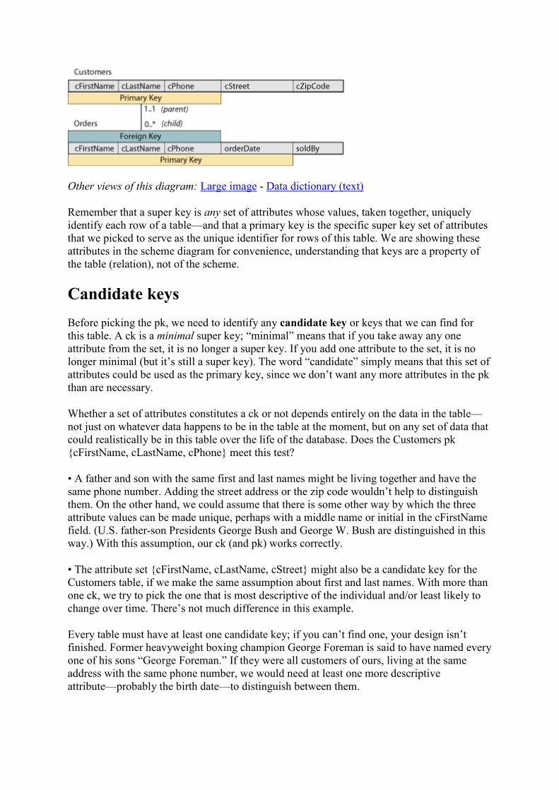
Other views of this diagram: Large image - Data dictionary (text)
Remember that a super key is any set of attributes whose values, taken together, uniquely
identify each row of a table—and that a primary key is the specific super key set of attributes
that we picked to serve as the unique identifier for rows of this table. We are showing these
attributes in the scheme diagram for convenience, understanding that keys are a property of
the table (relation), not of the scheme.
Candidate keys
Before picking the pk, we need to identify any candidate key or keys that we can find for
this table. A ck is a minimal super key; “minimal” means that if you take away any one
attribute from the set, it is no longer a super key. If you add one attribute to the set, it is no
longer minimal (but it’s still a super key). The word “candidate” simply means that this set of
attributes could be used as the primary key, since we don’t want any more attributes in the pk
than are necessary.
Whether a set of attributes constitutes a ck or not depends entirely on the data in the table—
not just on whatever data happens to be in the table at the moment, but on any set of data that
could realistically be in this table over the life of the database. Does the Customers pk
{cFirstName, cLastName, cPhone} meet this test?
• A father and son with the same first and last names might be living together and have the
same phone number. Adding the street address or the zip code wouldn’t help to distinguish
them. On the other hand, we could assume that there is some other way by which the three
attribute values can be made unique, perhaps with a middle name or initial in the cFirstName
field. (U.S. father-son Presidents George Bush and George W. Bush are distinguished in this
way.) With this assumption, our ck (and pk) works correctly.
• The attribute set {cFirstName, cLastName, cStreet} might also be a candidate key for the
Customers table, if we make the same assumption about first and last names. With more than
one ck, we try to pick the one that is most descriptive of the individual and/or least likely to
change over time. There’s not much difference in this example.
Every table must have at least one candidate key; if you can’t find one, your design isn’t
finished. Former heavyweight boxing champion George Foreman is said to have named every
one of his sons “George Foreman.” If they were all customers of ours, living at the same
address with the same phone number, we would need at least one more descriptive
attribute—probably the birth date—to distinguish between them.

PK size might matter
You’re probably thinking that it’s a real nuisance and waste of space to copy all three of the
Customer pk attributes to make the fk in Orders. If so, you’re right. Remember that we
purposely designed the Customers table without considering its association with Orders. Now
that it’s the parent in a one-to-many association, we have to ask if the pk is small enough to
be copied into the child table. In some tables, it will be— so we’re done. In this one, it isn’t—
so we’ll have to make up a pk that is small enough. There are two types of “made up”
primary keys:
• A surrogate PK is a single, small attribute (such as a number) that has no descriptive
value—it doesn’t tell us anything about the real-world individual. Most ID numbers are like
this. Surrogate keys are created for the convenience of the database designer (only). They are
a nuisance for database users, and should normally be hidden by the user interface of a
database system.
• A substitute PK is a single, small attribute (such as an abbreviation) that has at least some
descriptive value. Examples of substitute keys include the two-letter postal codes for the
states of the United States and the three-letter codes for worldwide airports. Substitute keys
are also created for the convenience of the database designer. They are frequently still a
nuisance for database users, although perhaps less so than surrogate PKs.
Do not automatically add “ID numbers” (surrogate keys) or substitute keys to a table until
you are sure that:
• There is at least one candidate key (before the surrogate is added),
• the table is a parent in at least one association, and
• there is no candidate key small enough for its values to be copied many times into the child
table.
These rules apply to surrogate and substitute keys that you (and your co-workers) add to your
own tables. However, you might find that a class type already has an attribute that appears to
be a surrogate or substitute key, but has been defined by someone else—usually a standards-
setting organization or a government agency. We call this attribute an external key. In the
external organization’s database, there is a candidate key for it, whether or not you have
access to it or include its value(s) in your own database. You may use it as a descriptive
attribute in both UML and the relation scheme diagram. Like other descriptive attributes, it
might or might not become part of a candidate key in your database. We will encounter many
of these (such as the zip code, UPC, and ISBN) in our examples.
• There is one special case of an external key that requires careful handling in your database
design: the United States social security number (SSN). Originally intended for use only to
identify social security participants, it has now become so over-used as an identifier that
access to it poses risks of serious damage to individuals, even including identity theft. Please
do not ever use the SSN in your database unless you are required to do so by law (for
example, to file tax information). Even then, do not use it as a primary key that would be
viewable to everyone who can access your database.
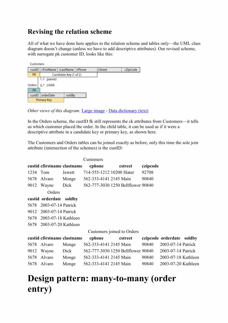
Revising the relation scheme
All of what we have done here applies to the relation scheme and tables only—the UML class
diagram doesn’t change (unless we have to add descriptive attributes). Our revised scheme,
with surrogate pk customer ID, looks like this:
Other views of this diagram: Large image - Data dictionary (text)
In the Orders scheme, the custID fk still represents the ck attributes from Customers—it tells
us which customer placed the order. In the child table, it can be used as if it were a
descriptive attribute in a candidate key or primary key, as shown here.
The Customers and Orders tables can be joined exactly as before, only this time the sole join
attribute (intersection of the schemes) is the custID:
Customers
custid cfirstname clastname cphone cstreet czipcode
1234 Tom Jewett 714-555-1212 10200 Slater 92708
5678 Alvaro Monge 562-333-4141 2145 Main 90840
9012 Wayne Dick 562-777-3030 1250 Bellflower 90840
Orders
custid orderdate soldby
5678 2003-07-14 Patrick
9012 2003-07-14 Patrick
5678 2003-07-18 Kathleen
5678 2003-07-20 Kathleen
Customers joined to Orders
custid cfirstname clastname cphone cstreet czipcode orderdate soldby
5678 Alvaro Monge 562-333-4141 2145 Main 90840 2003-07-14 Patrick
9012 Wayne Dick 562-777-3030 1250 Bellflower 90840 2003-07-14 Patrick
5678 Alvaro Monge 562-333-4141 2145 Main 90840 2003-07-18 Kathleen
5678 Alvaro Monge 562-333-4141 2145 Main 90840 2003-07-20 Kathleen
Design pattern: many-to-many (order
entry)

There are some modeling situations that you will find over and over again as you design real
databases. We refer to these as design patterns. If you understand the concepts behind each
one, you will in effect be adding new “tools” to your design toolbox that you can use in
building the model of an enterprise.
Our sales database represents one of these patterns. So far, we have customers and orders. To
finish the pattern, we need products to sell. We’ll first describe what the Product class means,
and how it is associated with the Order class:
“A product is a specific type of item that we have for sale. Each product has a descriptive
name; we distinguish similar products by the manufacturer's name and model number. For
each product, we need to know its unit list price and how many units of this product we have
in stock.”
• It is important to understand exactly what this class means: an example product might be
named “Blender, Commercial, 1.25 Qt.”, manufactured by Hamilton Beach, model number
908. This is a type of product, not an individual boxed blender that is sitting on our shelves.
The same manufacturer probably has different blender models (909, 918, 919), and there are
probably blenders that we stock that are made by other companies. Each would be a different
instance of this class.
“Each Order contains one or more Products.” (At least one because it doesn't make sense to
place an order for no products.)
“Each Product is contained in zero or more Orders.” (Zero because we might not have sold
any of this product yet.)
Since the maximum multiplicity in each direction is “many,” this is called a many-to-many
association between Orders and Products.
Each time an order is placed for a product, we need to know how many units of that product
are being ordered and what price we are actually selling the product for. (The sale price might
vary from the list price by customer discount, special sale, etc.) These attributes are a result
of the association between the Order and the Product. We show them in an association class
that is connected to the association by a dotted line. If there are no attributes that result from a
many-to-many association, there is no association class.
Class diagram
Other views of this diagram: Large image - Data dictionary (text)
There are two additional attributes shown in the class diagram that we haven’t talked about
yet. We need to know the subtotal for each order line (that is, the quantity times the unit sale
price) and the total dollar value of each order (the sum of the subtotals for each line in that
order). Since these values can be computed, they don’t need to be stored in the database, and
they are not included in the relation scheme. Their names in the class diagram are preceeded
by a “/” to show that they are derived attributes.
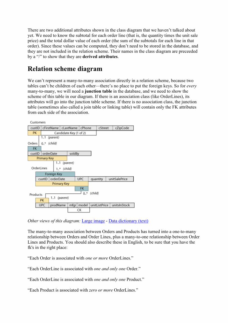
Relation scheme diagram
We can’t represent a many-to-many association directly in a relation scheme, because two
tables can’t be children of each other—there’s no place to put the foreign keys. So for every
many-to-many, we will need a junction table in the database, and we need to show the
scheme of this table in our diagram. If there is an association class (like OrderLines), its
attributes will go into the junction table scheme. If there is no association class, the junction
table (sometimes also called a join table or linking table) will contain only the FK attributes
from each side of the association.
Other views of this diagram: Large image - Data dictionary (text)
The many-to-many association between Orders and Products has turned into a one-to-many
relationship between Orders and Order Lines, plus a many-to-one relationship between Order
Lines and Products. You should also describe these in English, to be sure that you have the
fk's in the right place:
“Each Order is associated with one or more OrderLines.”
“Each OrderLine is associated with one and only one Order.”
“Each OrderLine is associated with one and only one Product.”
“Each Product is associated with zero or more OrderLines.”
With Orders now a parent of OrderLines, we might have decided that it needs a surrogate key
(order number) to be copied into the OrderLines. In fact, most sales systems do this, as you
know if you’ve ever tried to check on the status of something you’ve ordered from a
company. For this example, it seems to be just as easy to stick with the existing pk of Orders,
since it already has a surrogate key from Customers, and the order date doesn’t add much
size.
The UPC (Universal Product Code) is an external key. UPCs are defined for virtually all
grocery and manufactured products by a commercial organization called the Uniform Code
Council, Inc.® We will use it as the primary key of our Products table, which also has a
candidate key here: {mfgr, model}.
To uniquely identify each order line, we need to know both which order this line is contained
in, and which product is being ordered on this line. The two fk's, from Orders and Products,
together form the only candidate key of this relation and therefore the primary key. There is
no need to look for a smaller pk, since OrderLines has no children.
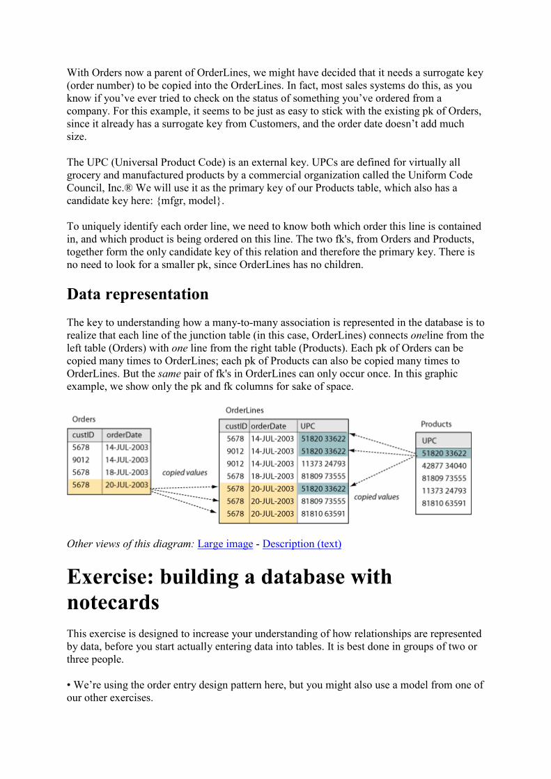
Data representation
The key to understanding how a many-to-many association is represented in the database is to
realize that each line of the junction table (in this case, OrderLines) connects oneline from the
left table (Orders) with one line from the right table (Products). Each pk of Orders can be
copied many times to OrderLines; each pk of Products can also be copied many times to
OrderLines. But the same pair of fk's in OrderLines can only occur once. In this graphic
example, we show only the pk and fk columns for sake of space.
Other views of this diagram: Large image - Description (text)
Exercise: building a database with
notecards
This exercise is designed to increase your understanding of how relationships are represented
by data, before you start actually entering data into tables. It is best done in groups of two or
three people.
• We’re using the order entry design pattern here, but you might also use a model from one of
our other exercises.

• Divide a stack of blank notecards into three groups. On one group, write data that represents
orders (one order per card). On the second group, write data that represents products (one
product per card). On the third group, write data that represents order lines (one order line per
card). Remember that you can’t make an order line without an order and a product (the
parents). You might also make a stack of Customer cards, and show how one customer can
place many orders.
• Use the format shown below. This is actually the UML notation for an object instance of a
class; however, we are adding the primary and foreign keys from the relation scheme (just as
you will do in the database). This may be a tedious bit of writing, but it will emphasize the
fact that object instances and database rows both are actually functions that assign domain
constants to attribute names.
• Use realistic data, but don’t just copy what we already have in the tables. Make enough
cards to show at least a few orders that include multiple order lines, and a few items that were
purchased on more than one order. Your cards should look like this:
Other views of this diagram: Large image - Description (text)
When you are finished, arrange the cards so that they show how order lines and products are
matched to the orders (or how orders and order lines are matched to products).
Design pattern: many-to-many with history
(the library loan)
Remember that the UML association class represents the attributes of a many-to-many
association, but can only be used if there is at most one pairing of any two individuals in the
relationship. This means, for example in order entry, that there can be only one order line for
each item ordered. This constraint is consistent with the enterprise being modeled.
• There are times when we need to allow the same two individuals in a many-to-many
association to be paired more than once. This frequently happens when we need to keep a
history of events over time.
Example: In a library, customers can borrow many books and each book can be borrowed by
many customers, so this seems to be a simple many-to-many association between customers
and books. But any one customer may borrow a book, return it, and then borrow the same
book again at a later time. The library records each book loan separately. There is no invoice
for each set of borrowed books and therefore no equivalent here of the Order in the order
entry example. (You have already seen other parts of the library model in exercises.)
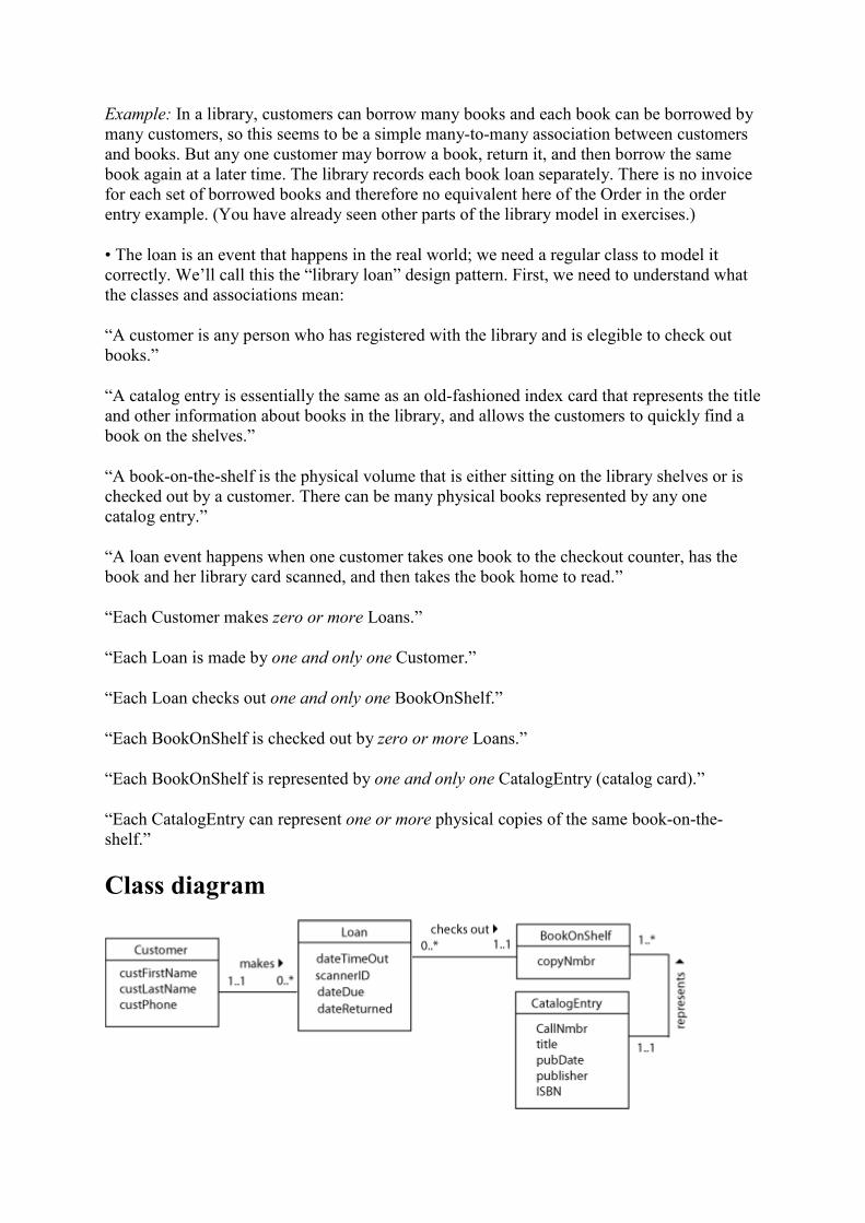
• The loan is an event that happens in the real world; we need a regular class to model it
correctly. We’ll call this the “library loan” design pattern. First, we need to understand what
the classes and associations mean:
“A customer is any person who has registered with the library and is elegible to check out
books.”
“A catalog entry is essentially the same as an old-fashioned index card that represents the title
and other information about books in the library, and allows the customers to quickly find a
book on the shelves.”
“A book-on-the-shelf is the physical volume that is either sitting on the library shelves or is
checked out by a customer. There can be many physical books represented by any one
catalog entry.”
“A loan event happens when one customer takes one book to the checkout counter, has the
book and her library card scanned, and then takes the book home to read.”
“Each Customer makes zero or more Loans.”
“Each Loan is made by one and only one Customer.”
“Each Loan checks out one and only one BookOnShelf.”
“Each BookOnShelf is checked out by zero or more Loans.”
“Each BookOnShelf is represented by one and only one CatalogEntry (catalog card).”
“Each CatalogEntry can represent one or more physical copies of the same book-on-the-
shelf.”
Class diagram

Other views of this diagram: Large image - Data dictionary (text)
Relation scheme diagram
As in the order entry example, the Customers table will need a surrogate key (added by us) to
save space when it is copied in the Loans. The CatalogEntries scheme already has two
external keys: the call number and the ISBN (International Standard Book Number). The first
of these is defined by the Library of Congress Classification system, and contains codes that
represent the subject, author, and year published. The second of these is defined by an ISO
(International Standards Organization) standard, number 2108. We’ll use the callNmbr as the
primary key, since it has more descriptive value than the ISBN and is smaller than the
descriptive CK {title, pubDate}.
Other views of this diagram: Large image - Data dictionary (text)
• As we would do in a junction table scheme, we’ll copy the primary key attributes from both
the Customers and the BooksOnShelf into the Loans scheme. This tells us which customer
borrowed which book, but it doesn't tell when it was borrowed; we have to know the
dateTimeOut in order to pair a customer with the same book more than once. We can call this
a discriminator attribute, since it allows us to discriminate between the multiple pairings of
customer and book. If you refer back to the UML class diagram, you’ll see that the loan,
which would have been a many-to-many association class between customers and books, has
become a “real” class because of the discriminator attribute.
• In most cases like this, we would use both FKs plus the discriminator attribute dateTimeOut
as PK of the Loans; here we need only the FK from the BooksOnShelf and the dateTimeOut
(since it is physically impossible to run the same book through the scanner more than once at
a time). Notice that there is actually another CK for loans: {dateTimeOut, scannerID}, since
it is also physically impossible for the same scanner to read two different books at exactly the
same time. We chose {callNmbr, copyNmbr, dateTimeOut} because it has just a bit more
descriptive value and because we don’t care about size here (since the Loan has no children).
Exercise: employee timecards
In many businesses, employees may work on a number of different projects. Each week, they
will submit a time card that lists each project on a separate line, along with the number of
hours that they have worked that week on that project.
• Describe each class in English.
• Draw the class diagram, including association classes if required.
• Describe each association in English (both directions).
• Draw the relation scheme.
The solution to this exercise will be discussed in class or posted online at a later date.
[
Design pattern: subkeys (the zip code)
(Wayne Dick and Tom Jewett)
One of the major goals of relational database design is to prevent unnecessary duplication of
data. In fact, this is one of the main reasons for using a relational database instead of a “flat
file” that stores all information in one table. Sometimes we will design a class that seems to
be correct, only to find out in the relation scheme or in the table itself that we have a problem.
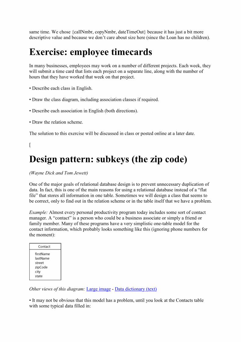
Example: Almost every personal productivity program today includes some sort of contact
manager. A “contact” is a person who could be a business associate or simply a friend or
family member. Many of these programs have a very simplistic one-table model for the
contact information, which probably looks something like this (ignoring phone numbers for
the moment):
Other views of this diagram: Large image - Data dictionary (text)
• It may not be obvious that this model has a problem, until you look at the Contacts table
with some typical data filled in:

Contacts
first,ame last,ame street zipCode city state
George Barnes 1254 Bellflower 90840 Long Beach CA
Susan Noble 1515 Palo Verde 90840 Long Beach CA
Erwin Star 17022 Brookhurst 92708 Fountain Valley CA
Alice Buck 3884 Atherton 90836 Long Beach CA
Frank Borders 10200 Slater 92708 Fountian Valley CA
Hanna Diedrich 1699 Studebaker 90840 Long Beach CA
• Notice the repeated information in the city and state attributes. This is not only redundant
data; it might also be inconsistent data. (Can you spot the “typo” above?)
Functional dependencies, subkeys, and lossless join
decomposition
To understand why we have a problem, we first have to understand the concept of a
functional dependency (FD), which is simply a more formal term for the super key property.
If X and Y are sets of attributes, then the notation X→Y is read “X functionally determines
Y” or “Y is functionally dependent on X.” This means that if I’m given a table filled with
data plus the value of the attributes in X, then I can uniquely determine the value of the
attributes in Y.
• A super key always functionally determines all of the other attributes in a relation (as well
as itself). This is a “good” FD. A “bad” FD happens when we have an attribute or set of
attributes that are a super key for some of the other attributes in the relation, but not a super
key for the entire relation. We call this set of attributes a subkey of the relation.
• In our example above, the zipCode is a subkey of the Contacts table. It is not a super key for
the entire table, but it functionally determines the city and state. (If you know the zip code,
you can always find the city and state, although you might need all nine digits instead of the
five we show here.) The opposite is not true, because many cities have more than one zip
code, like Long Beach in this example. We can show this in the relation scheme:
Other views of this diagram: Large image - Data dictionary (text)
• There is a very simple 3-step way to fix the problem with the relation scheme.
1. Remove all of the attributes that are dependent on the subkey. Put them into a new scheme.
In this example, the dependent attributes are the city and state.

2. Duplicate the subkey attribute set in the new scheme, where it becomes the primary key of
the new scheme. In this example, the sole subkey attribute is the zipCode.
3. Leave a copy of the subkey attribute set in the original scheme, where it is now a foreign
key. It is no longer a subkey, because you’ve gotten rid of the attributes that were
functionally dependent on it, and you’ve made it the primary key of its own table. The
revised model will have a many-to-one relationship between the original scheme and the new
one:
Other views of this diagram: Large image - Data dictionary (text)
• The new Contacts table will look like the old one, minus the city and state fields. The new
ZipLocations table, shown below, contains only one row per zip code. Joining this table to
the Contacts (on matching zipCode pk-fk pairs) will produce the same information that was
in the original table. What we have done is formally called lossless join decomposition of
the original table.
Zip locations
zipCode city state
90840 Long Beach CA
90836 Long Beach CA
92708 Fountain Valley CA
Subkeys and normalization
,ormalization means following a procedure or set of rules to insure that a database is well
designed. Most normalization rules are meant to eliminate redundant data (that is,
unnecessary duplicate data) in the database. Subkeys always result in redundant data, so we
need to eliminate them using the procedure outlined above.
• If there are no subkeys in any of the tables in your database, you have a well-designed
model according to what is usually called third normal form, or 3NF. Actually, 3NF permits
subkeys in some very exceptional circumstances that we won’t discuss here; the strict no-
subkey form is formally known as Boyce-Codd normal form, or BC,F.
• Some textbooks use the terms partial FDs and transitive FDs. Both of these are subkeys—
the first where the subkey is part of a primary key, the second where is isn’t. Both can be
eliminated by the procedure that we’ve shown here.

Correcting the UML class diagram
When we find a subkey in a relation scheme or table, we also know that the original UML
class was badly designed. The problem, always, is that we have actually placed two
conceptually different classes in a single class definition.
• In this example, a zipCode is not just an attribute of the Contact class. It is part of a
ZipLocation class, which we can describe as “a geographical location whose boundaries have
been uniquely identified by the U.S Postal Service for mail delivery.”
• The zipCode is an external key, created by the USPS for the convenience of its sorting
machinery (not the postal customers). The ZipLocation class has the additional attributes of
the city and state where it is located; in fact, it also has the attributes needed to precisely
describe its boundaries, although we certainly do not need to represent these in our database.
The geographical boundaries would form the “real” descriptive CK if they were included. As
always, we need to describe the association between ZipLocations and Contacts:
“Each Contact lives in one and only one ZipLocation”
“Each ZipLocation is home to zero or more Contacts”
• As with all one-to-many associations, the association itself identifies which Contact lives in
which ZipLocation. If we had started with this class diagram, we would have produced
exactly the same relation scheme that we developed with the normalization process above!
Other views of this diagram: Large image - Data dictionary (text)
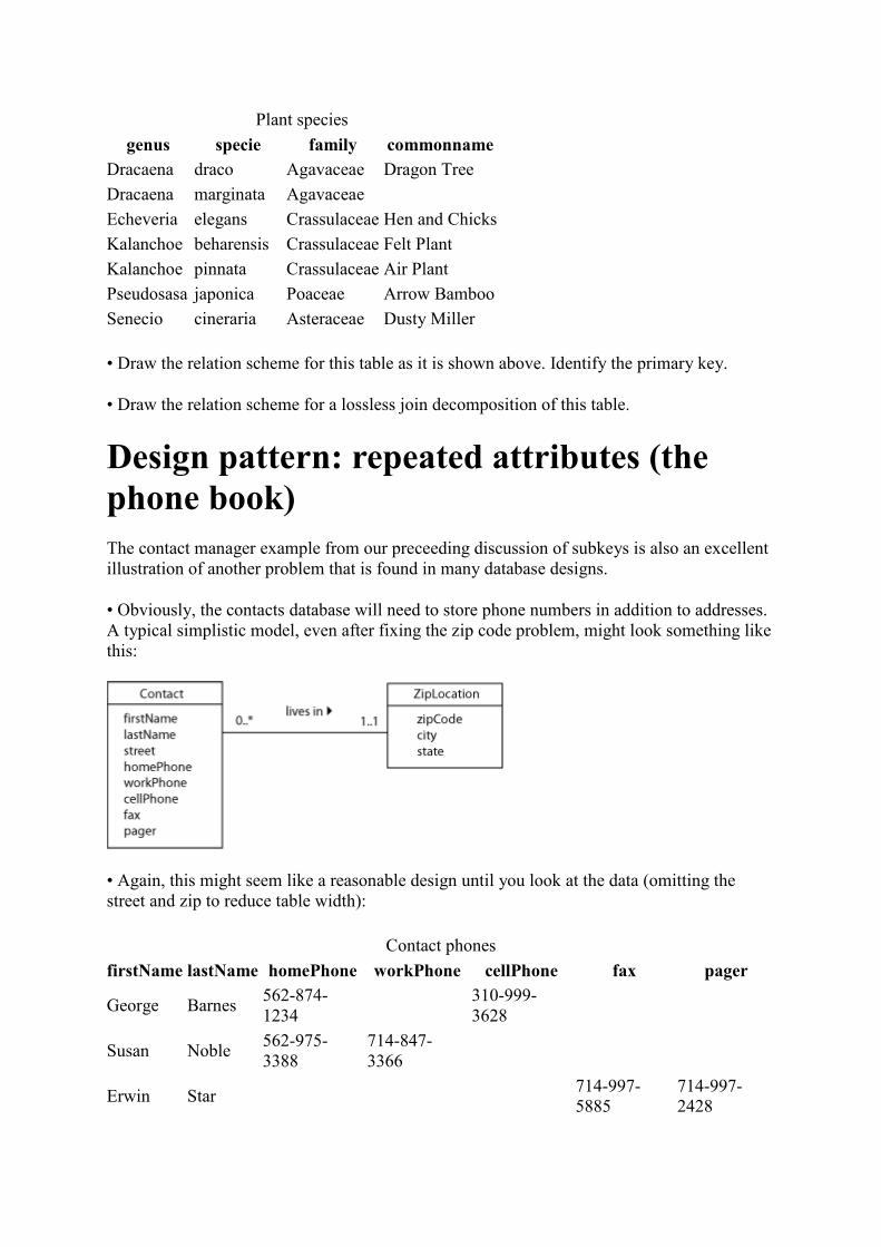
Exercise: plant species
You are working on a database for a company that grows and sells plants. One important
table contains a list of the plant species that they grow, which are identified botanically by
their genus and specie name, family, and common name. Even if you have never heard of
these terms, you can analyze the table by looking at the data given below:
Plant species
genus specie family commonname
Ardesia japonica Myrsinaceae Marlberry
Beaucarnea recurvata Agavaceae Ponytail
Centaurea cineraria Asteraceae Dusty Miller
Centaurea gymnocarpa Asteraceae Dusty Miller
Centaurea montana Asteraceae
Plant species
genus specie family commonname
Dracaena draco Agavaceae Dragon Tree
Dracaena marginata Agavaceae
Echeveria elegans Crassulaceae Hen and Chicks
Kalanchoe beharensis Crassulaceae Felt Plant
Kalanchoe pinnata Crassulaceae Air Plant
Pseudosasa japonica Poaceae Arrow Bamboo
Senecio cineraria Asteraceae Dusty Miller
• Draw the relation scheme for this table as it is shown above. Identify the primary key.
• Draw the relation scheme for a lossless join decomposition of this table.
Design pattern: repeated attributes (the
phone book)
The contact manager example from our preceeding discussion of subkeys is also an excellent
illustration of another problem that is found in many database designs.
• Obviously, the contacts database will need to store phone numbers in addition to addresses.
A typical simplistic model, even after fixing the zip code problem, might look something like
this:
• Again, this might seem like a reasonable design until you look at the data (omitting the
street and zip to reduce table width):
Contact phones
first,ame last,ame homePhone workPhone cellPhone fax pager
George Barnes 562-874-
1234
310-999-
3628
Susan Noble 562-975-
3388
714-847-
3366
Erwin Star
714-997-
5885
714-997-
2428
Contact phones
first,ame last,ame homePhone workPhone cellPhone fax pager
Alice Buck
562-577-
1200
562-561-
1921
Frank Borders 714-968-
8201
Hanna Diedrich
562-786-
7727
• There are at least two very large problems here:
- None of our contacts are going to have all of the phone numbers that we've provided for. In
fact, most contacts will have only one or two numbers—leaving most of these fields blank, or
NULL. Remember that ,ULL is a special constant value in database systems that means
“this field doesn’t have any value assigned to it.” It’s not the same as a zero length string or
the number zero. In general, we want to eliminate unnecessary NULL values that might occur
as a result of our design—and the NULL values in this table are definitely unnecessary.
- No matter how many phone number fields we provide (five of them here), sooner or later
someone will think of another kind of phone number that we need. With the model above, we
would have to actually change the table structure to add another field. Any information like
this that might change should be represented by data in a table rather than by the table
structure.
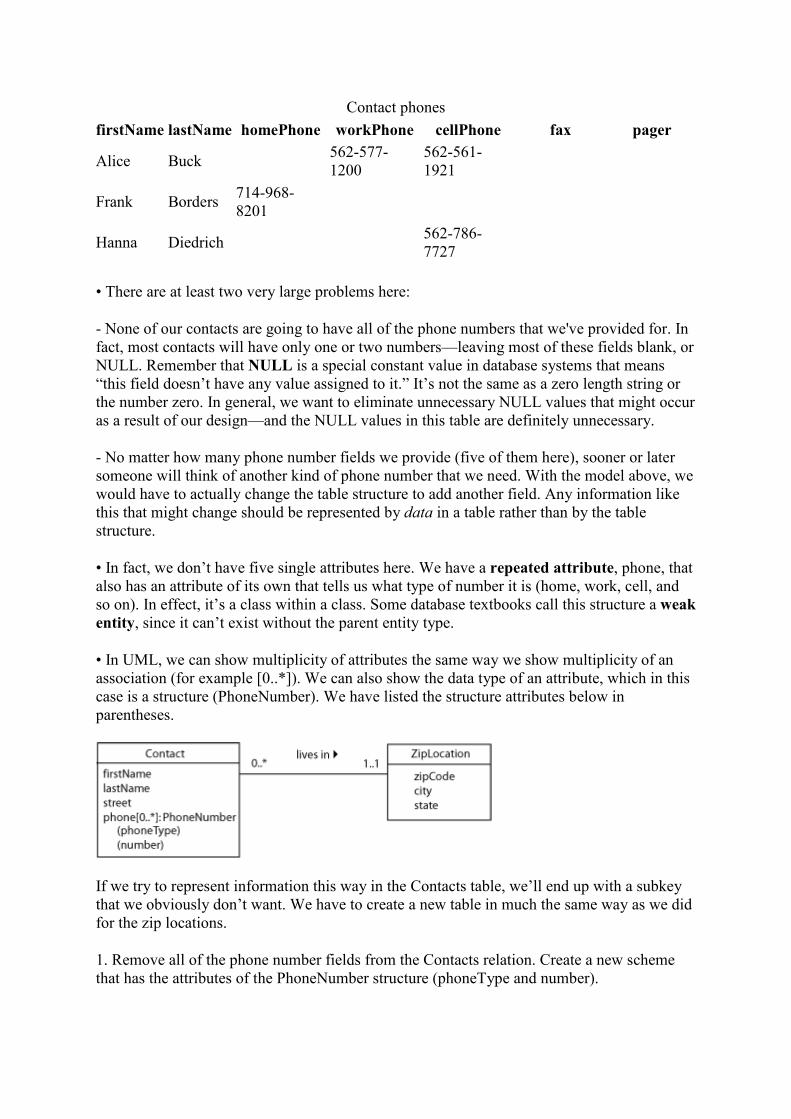
• In fact, we don’t have five single attributes here. We have a repeated attribute, phone, that
also has an attribute of its own that tells us what type of number it is (home, work, cell, and
so on). In effect, it’s a class within a class. Some database textbooks call this structure a weak
entity, since it can’t exist without the parent entity type.
• In UML, we can show multiplicity of attributes the same way we show multiplicity of an
association (for example [0..*]). We can also show the data type of an attribute, which in this
case is a structure (PhoneNumber). We have listed the structure attributes below in
parentheses.
If we try to represent information this way in the Contacts table, we’ll end up with a subkey
that we obviously don’t want. We have to create a new table in much the same way as we did
for the zip locations.
1. Remove all of the phone number fields from the Contacts relation. Create a new scheme
that has the attributes of the PhoneNumber structure (phoneType and number).
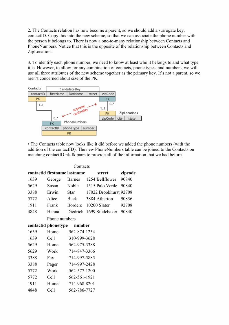
2. The Contacts relation has now become a parent, so we should add a surrogate key,
contactID. Copy this into the new scheme, so that we can associate the phone number with
the person it belongs to. There is now a one-to-many relationship between Contacts and
PhoneNumbers. Notice that this is the opposite of the relationship between Contacts and
ZipLocations.
3. To identify each phone number, we need to know at least who it belongs to and what type
it is. However, to allow for any combination of contacts, phone types, and numbers, we will
use all three attributes of the new scheme together as the primary key. It’s not a parent, so we
aren’t concerned about size of the PK.
• The Contacts table now looks like it did before we added the phone numbers (with the
addition of the contactID). The new PhoneNumbers table can be joined to the Contacts on
matching contactID pk-fk pairs to provide all of the information that we had before.
Contacts
contactid firstname lastname street zipcode
1639 George Barnes 1254 Bellflower 90840
5629 Susan Noble 1515 Palo Verde 90840
3388 Erwin Star 17022 Brookhurst 92708
5772 Alice Buck 3884 Atherton 90836
1911 Frank Borders 10200 Slater 92708
4848 Hanna Diedrich 1699 Studebaker 90840
Phone numbers
contactid phonetype number
1639 Home 562-874-1234
1639 Cell 310-999-3628
5629 Home 562-975-3388
5629 Work 714-847-3366
3388 Fax 714-997-5885
3388 Pager 714-997-2428
5772 Work 562-577-1200
5772 Cell 562-561-1921
1911 Home 714-968-8201
4848 Cell 562-786-7727
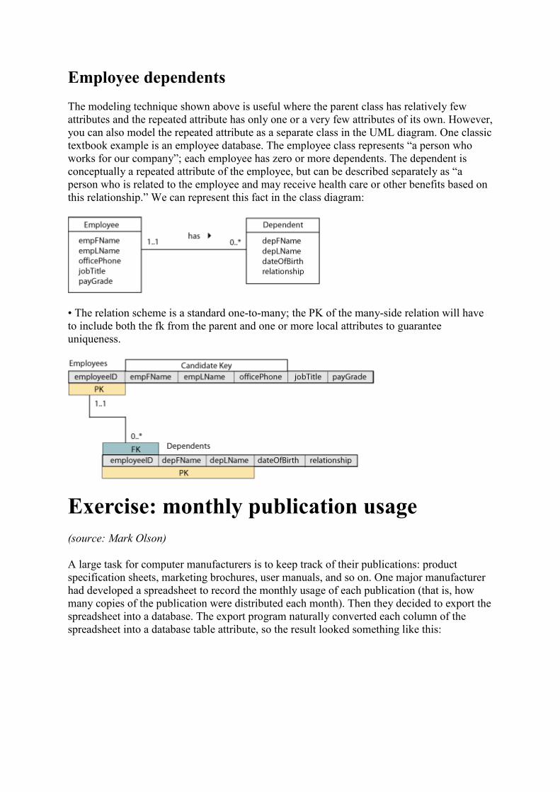
Employee dependents
The modeling technique shown above is useful where the parent class has relatively few
attributes and the repeated attribute has only one or a very few attributes of its own. However,
you can also model the repeated attribute as a separate class in the UML diagram. One classic
textbook example is an employee database. The employee class represents “a person who
works for our company”; each employee has zero or more dependents. The dependent is
conceptually a repeated attribute of the employee, but can be described separately as “a
person who is related to the employee and may receive health care or other benefits based on
this relationship.” We can represent this fact in the class diagram:
• The relation scheme is a standard one-to-many; the PK of the many-side relation will have
to include both the fk from the parent and one or more local attributes to guarantee
uniqueness.
Exercise: monthly publication usage
(source: Mark Olson)
A large task for computer manufacturers is to keep track of their publications: product
specification sheets, marketing brochures, user manuals, and so on. One major manufacturer
had developed a spreadsheet to record the monthly usage of each publication (that is, how
many copies of the publication were distributed each month). Then they decided to export the
spreadsheet into a database. The export program naturally converted each column of the
spreadsheet into a database table attribute, so the result looked something like this:

• Revise the class diagram to correct any problems that you find in this design. Then draw the
relation scheme for your corrected model.
Design pattern: multivalued attributes
(hobbies)
Attributes (like phone numbers) that are explicitly repeated in a class definition aren’t the
only design problem that we might have to correct. Suppose that we want to know what
hobbies each person on our contact list is interested in (perhaps to help us pick birthday or
holiday presents). We might add an attribute to hold these. More likely, someone else has
already built the database, and added this attribute without thinking about it.
• We’ve made this example obvious by using a plural name for the attribute, but this won’t
always be the case. We can only be sure that there’s a design problem when we see data in a
table that looks like this:
Contact hobbies
contactid firstname lastname hobbies
1639 George Barnes reading
5629 Susan Noble hiking, movies
3388 Erwin Star hockey, skiing
5772 Alice Buck
1911 Frank Borders photography, travel, art
4848 Hanna Diedrich gourmet cooking
• In this case, the hobby attribute wasn’t repeated in the scheme, but there are many distinct
values entered for it in the same column of the table. This is called a multivalued attribute.
The problem with doing it is that it is now difficult (but possible) to search the table for any
particular hobby that a person might have, and it is impossible to create a query that will

individually list the hobbies that are shown in the table. Unlike the phone book example,
NULL values are probably not part of the problem here, even if we don’t know the hobbies
for everyone in the database.
• In UML, we can again use the multiplicity notation to show that a contact may have more
than one hobby:
As you should expect by now, we can’t represent the multivalued attribute directly in the
Contacts relation scheme. Instead, we will remove the old hobbies attribute and create a new
scheme, very similar to the one that we created for the phone numbers.
• The relationship between Contacts and Hobbies is one-to-many, so we create the usual pk-
fk pair. The new scheme has only one descriptive attribute, the hobby name. To uniquely
identify each row of the table, we need to know both which contact this hobby belongs to and
which hobby it is—so both attributes form the pk of the scheme.
• With data entered, the new table looks similar to the PhoneNumbers. It can also be joined to
Contacts on matching pk-fk contactID pairs, re-creating the original data in a form that we
can now conveniently use for queries.
Hobbies
contactid hobby
1639 reading
5629 hiking
5629 movies
3388 hockey

Hobbies
contactid hobby
3388 skiing
1911 photography
1911 travel
1911 art
4848 gourmet cooking
Exercise: software list
Sometimes it takes more than just a glance at the class diagram to spot problems with a
design. Consider the following class type that might be used by a software vendor to list
software titles that are available.
• There is nothing obviously wrong with this design. However, the users of this database
might enter data that would cause problems, as shown in this table:
Software
TITLE VE,DOR PLATFORM VERSIO,
Wordy Macrosoft Win, Mac 9.4, 6.7
Visual B-- Macrosoft Win 6.0
Cherokee Open Source Linux, Solaris 10.4.5.2, 10.3.1.7
Inlook Hinkysoft Win, Linux, Palm OS 0.5
Corral Draw Corral Mac 22.1
• Revise the class diagram to correct any problems that you find in this design. Then draw the
relation scheme for your corrected model.
Discussion: more about domains
You learned earlier that a domain is the set of legal values that can be assigned to an attribute.
Each attribute in a database must have a well-defined domain; you can’t mix values from
different domains in the same attribute. (See below for some examples.) One goal of database
developers is to provide data integrity, part of which means insuring that the value entered
in each field of a table is consistent with its attribute domain. Sometimes we can devise a
validation rule to separate good from bad data; sometimes we can’t. Before you design the
data type and input format for an attribute, you have to understand the characteristics of its
domain.

• Some domains can only be described with a general statement of what they contain. These
are difficult or impossible to analyze precisely; the best we can do is to make them
VARCHAR strings that are long enough to hold any expected value. Examples include:
- Names of people. We typically show these broken into First (which might include a middle
name or initial) and Last (which is really the family name—some languages write this first).
Depending on your application, you might have to add attributes for a courtesy title (Mr.,
Ms., Dr., etc.), a suffix (Jr., III, etc.) or a nickname ('Tom' for 'Thomas' and so on).
- Names of businesses or organizations. These typically fit into a single character field, and
are not in the same domain as people’s names. Different domains require different attributes
(which sometimes can even mean different class/entity types).
- Street addresses. Even the format of these can vary widely: '3201 Main St., Apt. 3',
'Sohnmattstraße 14', and 'P.O. Box 8259' are all valid address strings.
• Some domains have at least some pattern in their permitted values. These might be
recognizable in code, for example with a regular expression, although it is still impossible to
insure that every value that passes a validity check is actually correct. Examples include:
- Email addresses. To be valid, an email address must contain a single @ sign that separates
the user name from the server and domain names. It cannot contain any spaces.
Unfortunately, that’s about all we can check.
- Web addresses (URLs). These form a different domain from email addresses or telephone
numbers, no matter how tempting it might be to permit any of them to be entered in the same
attribute field. Other than checking for spaces and other illegal characters, there’s again not
much way to be sure a URL is valid.
- North American telephone numbers. Many databases, and most wireless phones, require
numbers to be exactly ten digits—perhaps providing formatting such as (800)-555-1212.
Problem: you can't store extension numbers, access codes, or other data that has to be
transmitted along with the number itself. Solution: make this an unformatted character string
long enough to hold all the information that is needed.
• A very few domains conform to a precise pattern that can be analyzed or specified exactly.
Examples include:
- United States Social Security numbers. These are always of the form 999-99-9999, where 9
represents any digit.
- United States Zip codes, which are always of the form 99999 or 99999-9999. United States
state abbreviations are always of the form AA, where A is an upper-case letter; however, just
checking the format won’t insure a valid abbreviation. There is a much better way to model
this kind of domain, which we will explain separately.
- Definitely NOT international postal codes or phone numbers. Don’t ever over-specify a
domain or data entry field in any way that would prevent users from entering a valid real-life
domain value.

• Easy domains to handle are those which can be specified by a well-defined, built-in system
data type. These include integers, real numbers, and dates/times. You might have to range-
check these data types to insure that realistic values are entered. In most systems, a boolean
data type is also available; oddly, Oracle® doesn’t provide this. (Oracle developers typically
use a CHAR(1) data type, and assign it values of 'T' or 'F').
• Finally, there are many domains that may be specified by a well-defined, reasonably-sized
set of constant values. We’ll look at these in a separate page.
In general, your user interface should provide any necessary format or range checking. If
done well, this can help the user with data entry, increase data integrity, and prevent the user
from having to deal with cryptic and frustrating error messages from the database itself.
Design pattern: enumerated domains
Attribute domains that may be specified by a well-defined, reasonably-sized set of constant
values are called enumerated domains. You might know all of the values of the domain at
design time, or you might not. In either case, you should keep the entire list of values in a
separate table. Tables that are created for this purpose might be called enumeration tables,
dictionary tables, lookup tables, or domain-control tables or entities in some textbooks and
database software systems. Once in the database, they are no different from any other table;
PKs and FKs link them to other tables as always. There are a number of ways to design these
tables, from which the designer can choose the most appropriate for a particular attribute in a
particular class.
• Many students ask if this technique will create too many tables and query joins. The answer
is: “No.” Design the database as well as you can—if you have to “break the rules” later for
faster performance, you can always do so. In most designs, the drawbacks of any additional
table or tables are overwhelmed by their advantages:
- You can read the values from the table into a combo box, list box, or similar input control
on either a Web page or a GUI form. This allows the user to easily select only values that are
valid in this domain at this time.
- You can always update the table if new values are added to the domain, or if existing values
are changed. This is much easier than modifying your user-interface code or your table
structure.
1. In our earlier ZipLocations example, the state attribute clearly fits the definition of an
enumerated domain. In UML, we can simply use a data type specification to show this,
without adding a new class type.

• The relation scheme will show the table that contains the enumerated domain values. This
table might have a single attribute, or it might have two attributes: one for the true values and
one for a substitute key. Notice that the true values always form a candidate key of the table.
• For states, the second approach provides both the full name of the state and the U.S. Postal
Service abbreviation—a real benefit when it is time to design the user interface. Any time
that you can find an existing enumeration (external key), you should use it instead of making
up your own values. Besides the USPS state codes, examples include international airport
designators (like LAX, defined by the International Civil Aviation Organization) and web
top-level domains for countries (like CH or DE, called ccTLDs and defined by the Internet
Assigned Numbers Authority).
2. Multivalued attributes (for example, hobbies) might also have enumerated domains. We
can show this in the class diagram exactly as we did with a single-valued attribute:
• In the scheme, the relationship between Contacts and Hobbies has become many-to-many,
instead of one-to-many. This is shown in the scheme by linking an enumeration table to the
previous Hobbies table (which now functions like an association class).

Exercise: a pizza shop
.ote:This exercise might be started now and finished after you have covered subclasses, or
simply delayed until after that topic.
You are designing a database for a pizza shop that wants to get into Web-based sales. Your
client has given you the transcript of a typical phone order conversation:
Pizza shop associate (Lori): “Thank you for calling the Pizza Shop; this is Lori. How may I
help you?”
Caller (Rick): “What toppings do you put on your all-meat special?”
Lori: “Italian sausage, pepperoni, ground beef, salami, and bacon.”
Rick: “OK, I’d like a large one, but without the bacon.”
Lori: “Do you want regular crust, extra-thin, or whole wheat?”
Rick: “Regular is fine. And a medium wheat crust with just cheese.”
Lori: “We have mozzarella, parmesan, romano, smoked cheddar, and jalapeño jack.”
Rick: “Uhhh…just mozzarella and romano. What kind of sauce is on that?”
Lori: “Marinara, spicy southwestern, tandoori masala, or pesto—your choice.”
Rick: “Pesto sounds good.”
Lori: “You can add a large order of breadsticks for just 99 cents.”
Rick: “Sure, why not? And I'd like three small salads…” (muffled) “…make two of’em with
Italian dressing and one with ranch.”
Lori: “The dressing comes on the side; we’ll give you an extra one of each flavor. What
would you like to drink?”
Rick: “Keg’a beer, maybe?”
Lori: “Sorry, we just have soft drinks.”
Rick: (laughs) “Just kidding—how about two medium diet colas and a large iced tea.”
Lori: “That’s one large regular crust all-meat special, no bacon, one medium wheat crust with
pesto sauce, mozzarella and romano, one large order of breadsticks, three small salads, three
Italian dressing, two ranch, two medium diet colas and one large iced tea. Just a minute,
please…(cash register clicks several times)…your total with tax is 27 dollars and 39 cents. Is
this for pickup or delivery?”
Rick: “I’ll pick it up.”
Lori: “And your name?”
Rick: “Rick.”
Lori: “Thank you for your order, Rick. It’ll be ready in about 20 minutes.”
Rick: “See’ya then.”
• Develop a class diagram which will accommodate at least the information contained in this
conversation, then draw the relation scheme. Remember to describe each class, and the
associations between them, in English. Your system will have to let the sales associate (or
Web customer) select from the available current menu choices, and also let the sales associate
(or Web script) record the order.
Design pattern: subclasses
Top down design
As you are developing a class diagram, you might discover that one or more attributes of a
class are characteristics of only some individuals of that class, but not of others. This
probably indicates that you need to develop a subclass of the basic class type. We call the
process of designing subclasses from “top down” specialization; a class that represents a
subset of another class type can also be called a specialization of its parent class.
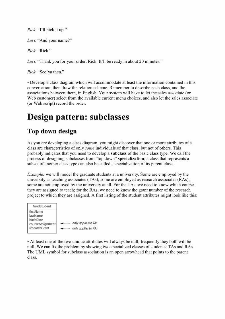
Example: we will model the graduate students at a university. Some are employed by the
university as teaching associates (TAs); some are employed as research associates (RAs);
some are not employed by the university at all. For the TAs, we need to know which course
they are assigned to teach; for the RAs, we need to know the grant number of the research
project to which they are assigned. A first listing of the student attributes might look like this:
• At least one of the two unique attributes will always be null; frequently they both will be
null. We can fix the problem by showing two specialized classes of students: TAs and RAs.
The UML symbol for subclass association is an open arrowhead that points to the parent
class.

• Unique attributes are now contained in the subclass types. Attributes that are common to all
students remain in the superclass (parent).
• The verbs to describe a subclass association are implied by the diagram. In this case, we
would say that each grad student may be either a TA, an RA, or neither; each TA or RA is a
grad student.
Specialization constraints
Rather than the usual cardinality/multiplicity symbols, the subclass association line is labeled
with specialization constraints. Constraints are described along two dimensions: incomplete
versus complete, and disjoint versus overlapping.
• In an incomplete specialization, also called a partial specialization, only some individuals
of the parent class are specialized (that is, have unique attributes). Other individuals of the
parent class have only the common attributes.
• In a complete specialization, all individuals of the parent class have one or more unique
attributes that are not common to the generalized (parent) class.
• In a disjoint specialization, also called an exclusive specialization, an individual of the
parent class may be a member of only one specialized subclass.
• In an overlapping specialization, an individual of of the parent class may be a member of
more than one of the specialized subclasses.
Relation scheme diagram
We create a table for each of the subclasses, linked to the parent class with a pk-fk pair as
always. Since the relationships are one-to-one, only the fk is needed to form the pk of the
subclass table. There is no way to enforce the specialization constraints in the table
structure—this has to be done by the data entry system. Notice that there is no attribute in the
parent table to tell us if a student is a TA, an RA, or neither—the union of two outer join
queries will produce a table with all of the information that we need.

Bottom up design
Sometimes, instead of finding unique attributes in a single class type, you might find two or
more classes that have many of the same attributes. This probably indicates that you need to
develop a superclass of the classes with common attributes. We call the process of designing
subclasses from “bottom up” generalization; a class or entity that represents a superset of
other class types can also be called a generalization of the child types. .ote: if you have two
or more class types with exactly the same set of attributes, you probably have only one class
type instead of many!
Example (thanks to Martin Malolepszy): A student of mine had a summer job with a brush-
clearing service. This is a fairly specialized business but an essential one in southern
California, where dried plant growth (brush) can present a severe fire hazard if it is not
cleared from around houses and other structures. In addition to his exhausting physical work,
Martin built a small database to help the owner manage this business.
• One important class type was the lot (or property) to be cleared. Some lots were in the city,
with a standard street-and-number address. Other lots were not on a city street, but were
described by the county surveyor's section and tract number. It seemed as if there were two
class types:
• Actually, a few of the lots were identified by both address schemes. A closer look at the city
and county lot classes also shows two common descriptive attributes (the owner and the lot
size). The common attributes should go in a generalization or superclass that is simply called
a “lot.” The relation scheme is identical in structure to the previous example.
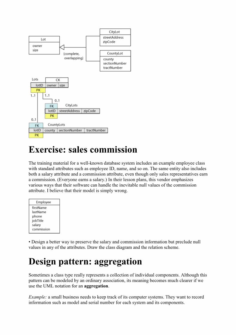
Exercise: sales commission
The training material for a well-known database system includes an example employee class
with standard attributes such as employee ID, name, and so on. The same entity also includes
both a salary attribute and a commission attribute, even though only sales representatives earn
a commission. (Everyone earns a salary.) In their lesson plans, this vendor emphasizes
various ways that their software can handle the inevitable null values of the commission
attribute. I believe that their model is simply wrong.
• Design a better way to preserve the salary and commission information but preclude null
values in any of the attributes. Draw the class diagram and the relation scheme.
Design pattern: aggregation
Sometimes a class type really represents a collection of individual components. Although this
pattern can be modeled by an ordinary association, its meaning becomes much clearer if we
use the UML notation for an aggregation.
Example: a small business needs to keep track of its computer systems. They want to record
information such as model and serial number for each system and its components.

• A very naïve way to do this would be to put all of the information into a single class type.
You should recognize that this class contains a set of repeated attributes with all of the
problems of the “phone book” pattern. You could fix it as we show here:
Incorrect model (with improvement)
• The improved model will accommodate the addition of more types of components (a
scanner, perhaps), a system with more than one monitor or printer, or a replacement
component on the shelf that don’t belong to any system right now. But UML allows us to
show the association in a more semantically correct way.
Better model (with UML aggregation)
• The system is an aggregation of components. In UML, aggregation is shown by an open
diamond on the end of the association line that points to the parent (aggregated) class. There
is an implied multiplicity on this end of 0..1, with multiplicity of the other end shown in the
diagram as usual. To describe this association, we would say that each system is composed of
one or more components and each component is part of zero or one system.
• Since the component can exist by itself in this model (without being part of a system), the
system name can’t be part of its PK. We'll use the only candidate key {type, mfgr, model,
SN} as PK, since this class is not a parent. The system name, just an FK here, will be filled in
if this component is installed as part of a system; it will be null otherwise.

In UML, there is a stronger form of aggregation that is called composition. The notation is
similar, using a filled-in diamond instead of an open one. In composition, component
instances cannot exist on their own without a parent; they are created with (or after) the
parent and they are deleted if the parent is deleted. The implied multiplicity on the “diamond”
end of the association is therefore 1..1.
Design pattern: recursive associations
A recursive association connects a single class type (serving in one role) to itself (serving in
another role).
Example: In most companies, each employee (except the CEO) is supervised by one
manager. Of course, not all employees are managers. This example is used in almost every
database textbook, since the association between employees and managers is relatively easy
to understand. Perhaps the best way to visualize it is to start with two class types:
Incorrect model
• The problem with this model is that each manager is also an employee. Building the second
(manager) table not only duplicates information from the employee table, it virtually
guarantees that there will be mistakes and conflicts in the data. We can fix the problem by
eliminating the redundant class and re-drawing the association line.
Correct model
• Normally, we wouldn’t show an fk in the class diagram; however, including the manager as
an attribute of the employee here (in addition to the association line) can help in
understanding the model. In the relation scheme, we can explicitly show the connection
between the surrogate pk (employeeID) and the managerID (which is an fk, even though it is
in the same scheme).
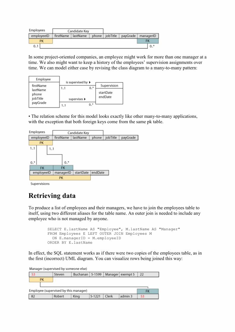
In some project-oriented companies, an employee might work for more than one manager at a
time. We also might want to keep a history of the employees’ supervision assignments over
time. We can model either case by revising the class diagram to a many-to-many pattern:
• The relation scheme for this model looks exactly like other many-to-many applications,
with the exception that both foreign keys come from the same pk table.
Retrieving data
To produce a list of employees and their managers, we have to join the employees table to
itself, using two different aliases for the table name. An outer join is needed to include any
employee who is not managed by anyone.
SELECT E.lastName AS "Employee", M.lastName AS "Manager"
FROM Employees E LEFT OUTER JOIN Employees M
ON E.managerID = M.employeeID
ORDER BY E.lastName
In effect, the SQL statement works as if there were two copies of the employees table, as in
the first (incorrect) UML diagram. You can visualize rows being joined this way:

The many-to-many structure is handled similarly in SQL. (Note the explicit ordering of the
joins specified by parentheses.):
SELECT E.lastName AS "Employee", M.lastName AS "Manager"
FROM Employees E LEFT OUTER JOIN
(Supervisions S INNER JOIN Employees M
ON S.managerID = M.employeeID)
ON E.employeeID = S.employeeID
ORDER BY E.lastName
Exercise: team games
You are modeling a sports league—it could be any team sport. Certainly one important class
is the team, which will have a name (unique within the league), a coach, a home field or
venue, and probably more attributes.
• Obviously, teams play games. In each game, there is a designated “home team” and “away
team” (even if the game is played at a neutral venue). Teams may play each other more than
once during a season, possibly even with the same home and away roles (for example, during
playoffs).
• Design a class diagram that shows the teams, the games that they play, and the score of each
game. Then draw the relation scheme for your model.
Appendix: traditional normalization
Normalization is usually thought of as a process of applying a set of rules to your database
design, mostly to achieve minimum redundancy in the data. Most textbooks present this as a
three-step process, with correspondingly labeled “normal forms,” which could be done in an
almost algorthmic sequence.
• In theory, you could start with a single relation scheme (sometimes called the universal
scheme, or U) that contains all of the attributes in the database—then apply these rules
recursively to develop a set of increasingly-normalized sub-relation schemes. When all of the
schemes are in third normal form, then the whole database is properly normalized. In
practice, you will more likely apply the rules gradually, refining each relation scheme as you
develop it from the UML class diagram or ER model diagram. The final table structures
should be the same no matter which method (or combination of methods) you’ve used.
• Since most developers will use traditional terms, you should know how the design patterns
that you have learned will lead to the same (normalized) results, as shown in the following
table:
Normal forms
,ormal form Traditional definition As presented here
First normal form
(1NF)
• All attributes must be
atomic, and
• No repeating groups
• Eliminate multi-valued attributes, and
• Eliminate repeated attributes

Normal forms
,ormal form Traditional definition As presented here
Second normal
form (2NF)
• First normal form, and
• No partial functional
dependencies
• Eliminate subkeys (where the subkey is part
of a composite primary key)
Third normal form
(3NF)
• Second normal form, and
• No transitive functional
dependencies
• Eliminate subkeys (where the subkey is not
part of the primary key)
• Some textbooks discuss “higher” normal forms, such as BCNF (Boyce-Codd), 4NF, 5NF,
and DKNF (domain-key). These topics are properly covered in a more advanced course or
tutorial.
Denormalization
One major premise of this tutorial is that you should learn to develop the “best” possible
design—which really focuses on the database structure itself. By doing this, you should be
able to avoid many of the problems, bugs, inconsistencies, and maintenance nightmares that
frequently plague actual systems in use today.
• However, your database will always be part of a larger system, which will include at least a
user interface and reporting structure, perhaps with a large amount of application code written
in a language such as Java or C++. Your database could also be the back-end of a Web site,
with both middle-tier business logic and front-end presentation code dependent on it. It is not
uncommon for developers to “break the rules” of database design in order to accommodate
other parts of a system.
• An example of denormalization, using our “phone book” problem, would be to store the
city and state attributes in the basic contacts table, rather than making a separate zip codes
table. At the cost of extra storage, this would save one join in a SELECT statement. Although
this would certainly not be needed in such a simple system, imagine a Web site that supports
thousands of “hits” per second, with much more complicated queries needed to produce the
output. With today’s terabyte disk systems, it might be worth using extra storage space to
keep Web viewers from waiting excessively while a page is being generated. On the other
hand, similarly-increasing processor power makes it less likely that this tradeoff will actually
have to be made in practice.
• The key to successful denormalization is to make sure that end users of the system never
have to manually duplicate or maintain the redundant data. Possible techniques for doing this
include using materialized views, writing triggers (code executed by the database itself—not
available on all systems), or writing application code that takes care of it at data-entry time.
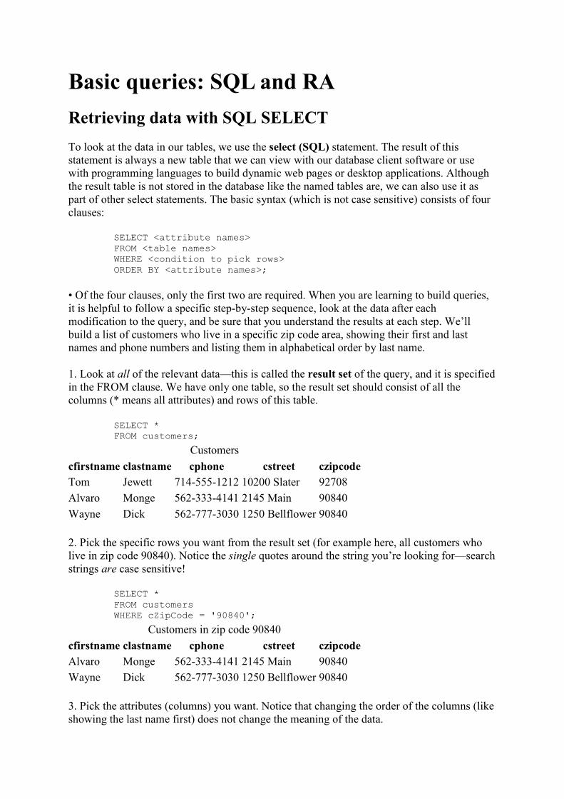
Basic queries: SQL and RA
Retrieving data with SQL SELECT
To look at the data in our tables, we use the select (SQL) statement. The result of this
statement is always a new table that we can view with our database client software or use
with programming languages to build dynamic web pages or desktop applications. Although
the result table is not stored in the database like the named tables are, we can also use it as
part of other select statements. The basic syntax (which is not case sensitive) consists of four
clauses:
SELECT <attribute names>
FROM <table names>
WHERE <condition to pick rows>
ORDER BY <attribute names>;
• Of the four clauses, only the first two are required. When you are learning to build queries,
it is helpful to follow a specific step-by-step sequence, look at the data after each
modification to the query, and be sure that you understand the results at each step. We’ll
build a list of customers who live in a specific zip code area, showing their first and last
names and phone numbers and listing them in alphabetical order by last name.
1. Look at all of the relevant data—this is called the result set of the query, and it is specified
in the FROM clause. We have only one table, so the result set should consist of all the
columns (* means all attributes) and rows of this table.
SELECT *
FROM customers;
Customers
cfirstname clastname cphone cstreet czipcode
Tom Jewett 714-555-1212 10200 Slater 92708
Alvaro Monge 562-333-4141 2145 Main 90840
Wayne Dick 562-777-3030 1250 Bellflower 90840
2. Pick the specific rows you want from the result set (for example here, all customers who
live in zip code 90840). Notice the single quotes around the string you’re looking for—search
strings are case sensitive!
SELECT *
FROM customers
WHERE cZipCode = '90840';
Customers in zip code 90840
cfirstname clastname cphone cstreet czipcode
Alvaro Monge 562-333-4141 2145 Main 90840
Wayne Dick 562-777-3030 1250 Bellflower 90840
3. Pick the attributes (columns) you want. Notice that changing the order of the columns (like
showing the last name first) does not change the meaning of the data.

SELECT cLastName, cFirstName, cPhone
FROM customers
WHERE cZipCode = '90840';
Columns from SELECT
cLast,ame cFirst,ame cPhone
Monge Alvaro 562-333-4141
Dick Wayne 562-777-3030
4. In SQL, you can also specify the order in which to list the results. Once again, the order in
which rows are listed does not change the meaning of the data in them.
SELECT cLastName, cFirstName, cPhone
FROM customers
WHERE cZipCode = '90840'
ORDER BY cLastName, cFirstName;
Rows in order
cLast,ame cFirst,ame cPhone
Dick Wayne 562-777-3030
Monge Alvaro 562-333-4141
Why SQL works: the RA select and project
Like all algebras, RA applies operators to operands to produce results. RA operands are
relations; results are new relations that can be used as operands in building more complex
expressions. We’ll introduce two of the RA operators following the example and sequence
above.
1. To represent a single relation in RA, we only need to use its name. We can also represent
relations and schemes symbolically with small and capital letters, for example relation r over
scheme R. In this case, r = customers and R = the Customers scheme.
2. The select (RA) operator (written σ) picks tuples, like the SQL WHERE clause picks rows.
It is a unary operator that takes a single relation or expression as its operand. It also takes a
predicate, θ, to specify which tuples are required. Its syntax is σθr, or in our example:
σcZipCode='90840'customers.
The scheme of the result of σθr is R—the same scheme we started with—since we haven’t
done anything to change the attribute list. The result of this operation includes all tuples of r
for which the predicate θ evaluates to true.
3. The project (RA) operator (written π) picks attributes, confusingly like the SQL SELECT
clause. It is also a unary operator that takes a single relation or expression as its operand.
Instead of a predicate, it takes a subscheme, X (of R), to specify which attributes are
required. Its syntax is πXr, or in our example:
πcLastName, cFirstName, cPhonecustomers.

The scheme of the result of πXr is X. The tuples resulting from this operation are tuples of
the original relation, r, cut down to the attributes contained in X.
• For X to be a subscheme of R, it must be a subset of the attributes in R, and preserve the
assignment rule from R (that is, each attribute of X must have the same domain as its
corresponding attribute in R).
• If X is a super key of r, then there will be the same number of tuples in the result as there
were to begin with in r. If X is not a super key of r, then any duplicate (non-distinct) tuples
are eliminated from the result.
Just as in the SQL statement, we can apply the project operator to the output of the select
operation to produce the results that we want: πXσθr or
πcLastName, cFirstName, cPhone σcZipCode='90840'customers.
Since RA considers relations strictly as sets of tuples, there is no way to specify the order of
tuples in a result relation.
Basic SQL statements: DDL and DML
In the first part of this tutorial, you’ve seen some of the SQL statements that you need to start
building a database. This page gives you a review of those and adds several more that you
haven’t seen yet.
• SQL statements are divided into two major categories: data definition language (DDL)
and data manipulation language (DML). Both of these categories contain far more
statements than we can present here, and each of the statements is far more complex than we
show in this introduction. If you want to master this material, we strongly recommend that
you find a SQL reference for your own database software as a supplement to these pages.
Data definition language
DDL statements are used to build and modify the structure of your tables and other objects in
the database. When you execute a DDL statement, it takes effect immediately.
• The create table statement does exactly that:
CREATE TABLE <table name> (
<attribute name 1> <data type 1>,
...
<attribute name n> <data type n>);
The data types that you will use most frequently are character strings, which might be called
VARCHAR or CHAR for variable or fixed length strings; numeric types such as NUMBER
or INTEGER, which will usually specify a precision; and DATE or related types. Data type
syntax is variable from system to system; the only way to be sure is to consult the
documentation for your own software.
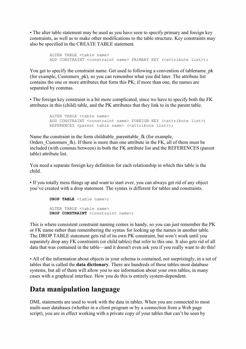
• The alter table statement may be used as you have seen to specify primary and foreign key
constraints, as well as to make other modifications to the table structure. Key constraints may
also be specified in the CREATE TABLE statement.
ALTER TABLE <table name>
ADD CONSTRAINT <constraint name> PRIMARY KEY (<attribute list>);
You get to specify the constraint name. Get used to following a convention of tablename_pk
(for example, Customers_pk), so you can remember what you did later. The attribute list
contains the one or more attributes that form this PK; if more than one, the names are
separated by commas.
• The foreign key constraint is a bit more complicated, since we have to specify both the FK
attributes in this (child) table, and the PK attributes that they link to in the parent table.
ALTER TABLE <table name>
ADD CONSTRAINT <constraint name> FOREIGN KEY (<attribute list>)
REFERENCES <parent table name> (<attribute list>);
Name the constraint in the form childtable_parenttable_fk (for example,
Orders_Customers_fk). If there is more than one attribute in the FK, all of them must be
included (with commas between) in both the FK attribute list and the REFERENCES (parent
table) attribute list.
You need a separate foreign key definition for each relationship in which this table is the
child.
• If you totally mess things up and want to start over, you can always get rid of any object
you’ve created with a drop statement. The syntax is different for tables and constraints.
DROP TABLE <table name>;
ALTER TABLE <table name> DROP CONSTRAINT <constraint name>;
This is where consistent constraint naming comes in handy, so you can just remember the PK
or FK name rather than remembering the syntax for looking up the names in another table.
The DROP TABLE statement gets rid of its own PK constraint, but won’t work until you
separately drop any FK constraints (or child tables) that refer to this one. It also gets rid of all
data that was contained in the table—and it doesn't even ask you if you really want to do this!
• All of the information about objects in your schema is contained, not surprisingly, in a set of
tables that is called the data dictionary. There are hundreds of these tables most database
systems, but all of them will allow you to see information about your own tables, in many
cases with a graphical interface. How you do this is entirely system-dependent.
Data manipulation language
DML statements are used to work with the data in tables. When you are connected to most
multi-user databases (whether in a client program or by a connection from a Web page
script), you are in effect working with a private copy of your tables that can’t be seen by
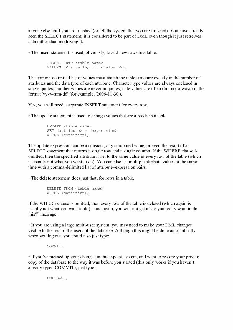
anyone else until you are finished (or tell the system that you are finished). You have already
seen the SELECT statement; it is considered to be part of DML even though it just retreives
data rather than modifying it.
• The insert statement is used, obviously, to add new rows to a table.
INSERT INTO <table name>
VALUES (<value 1>, ... <value n>);
The comma-delimited list of values must match the table structure exactly in the number of
attributes and the data type of each attribute. Character type values are always enclosed in
single quotes; number values are never in quotes; date values are often (but not always) in the
format 'yyyy-mm-dd' (for example, '2006-11-30').
Yes, you will need a separate INSERT statement for every row.
• The update statement is used to change values that are already in a table.
UPDATE <table name>
SET <attribute> = <expression>
WHERE <condition>;
The update expression can be a constant, any computed value, or even the result of a
SELECT statement that returns a single row and a single column. If the WHERE clause is
omitted, then the specified attribute is set to the same value in every row of the table (which
is usually not what you want to do). You can also set multiple attribute values at the same
time with a comma-delimited list of attribute=expression pairs.
• The delete statement does just that, for rows in a table.
DELETE FROM <table name>
WHERE <condition>;
If the WHERE clause is omitted, then every row of the table is deleted (which again is
usually not what you want to do)—and again, you will not get a “do you really want to do
this?” message.
• If you are using a large multi-user system, you may need to make your DML changes
visible to the rest of the users of the database. Although this might be done automatically
when you log out, you could also just type:
COMMIT;
• If you’ve messed up your changes in this type of system, and want to restore your private
copy of the database to the way it was before you started (this only works if you haven’t
already typed COMMIT), just type:
ROLLBACK;
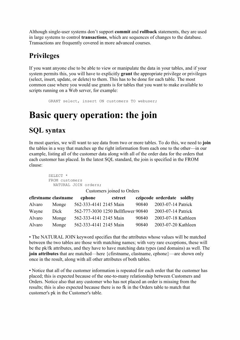
Although single-user systems don’t support commit and rollback statements, they are used
in large systems to control transactions, which are sequences of changes to the database.
Transactions are frequently covered in more advanced courses.
Privileges
If you want anyone else to be able to view or manipulate the data in your tables, and if your
system permits this, you will have to explicitly grant the appropriate privilege or privileges
(select, insert, update, or delete) to them. This has to be done for each table. The most
common case where you would use grants is for tables that you want to make available to
scripts running on a Web server, for example:
GRANT select, insert ON customers TO webuser;
Basic query operation: the join
SQL syntax
In most queries, we will want to see data from two or more tables. To do this, we need to join
the tables in a way that matches up the right information from each one to the other—in our
example, listing all of the customer data along with all of the order data for the orders that
each customer has placed. In the latest SQL standard, the join is specified in the FROM
clause:
SELECT *
FROM customers
NATURAL JOIN orders;
Customers joined to Orders
cfirstname clastname cphone cstreet czipcode orderdate soldby
Alvaro Monge 562-333-4141 2145 Main 90840 2003-07-14 Patrick
Wayne Dick 562-777-3030 1250 Bellflower 90840 2003-07-14 Patrick
Alvaro Monge 562-333-4141 2145 Main 90840 2003-07-18 Kathleen
Alvaro Monge 562-333-4141 2145 Main 90840 2003-07-20 Kathleen
• The NATURAL JOIN keyword specifies that the attributes whose values will be matched
between the two tables are those with matching names; with very rare exceptions, these will
be the pk/fk attributes, and they have to have matching data types (and domains) as well. The
join attributes that are matched—here {cfirstname, clastname, cphone}—are shown only
once in the result, along with all other attributes of both tables.
• Notice that all of the customer information is repeated for each order that the customer has
placed; this is expected because of the one-to-many relationship between Customers and
Orders. Notice also that any customer who has not placed an order is missing from the
results; this is also expected because there is no fk in the Orders table to match that
customer's pk in the Customer's table.
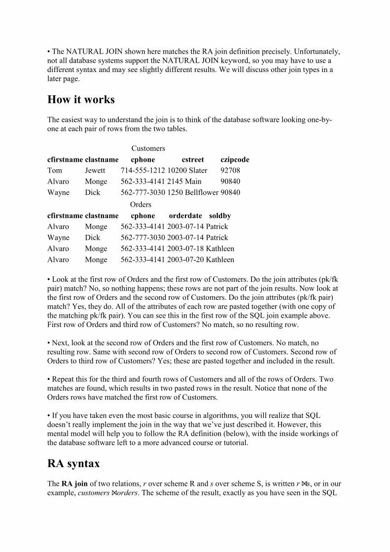
• The NATURAL JOIN shown here matches the RA join definition precisely. Unfortunately,
not all database systems support the NATURAL JOIN keyword, so you may have to use a
different syntax and may see slightly different results. We will discuss other join types in a
later page.
How it works
The easiest way to understand the join is to think of the database software looking one-by-
one at each pair of rows from the two tables.
Customers
cfirstname clastname cphone cstreet czipcode
Tom Jewett 714-555-1212 10200 Slater 92708
Alvaro Monge 562-333-4141 2145 Main 90840
Wayne Dick 562-777-3030 1250 Bellflower 90840
Orders
cfirstname clastname cphone orderdate soldby
Alvaro Monge 562-333-4141 2003-07-14 Patrick
Wayne Dick 562-777-3030 2003-07-14 Patrick
Alvaro Monge 562-333-4141 2003-07-18 Kathleen
Alvaro Monge 562-333-4141 2003-07-20 Kathleen
• Look at the first row of Orders and the first row of Customers. Do the join attributes (pk/fk
pair) match? No, so nothing happens; these rows are not part of the join results. Now look at
the first row of Orders and the second row of Customers. Do the join attributes (pk/fk pair)
match? Yes, they do. All of the attributes of each row are pasted together (with one copy of
the matching pk/fk pair). You can see this in the first row of the SQL join example above.
First row of Orders and third row of Customers? No match, so no resulting row.
• Next, look at the second row of Orders and the first row of Customers. No match, no
resulting row. Same with second row of Orders to second row of Customers. Second row of
Orders to third row of Customers? Yes; these are pasted together and included in the result.
• Repeat this for the third and fourth rows of Customers and all of the rows of Orders. Two
matches are found, which results in two pasted rows in the result. Notice that none of the
Orders rows have matched the first row of Customers.
• If you have taken even the most basic course in algorithms, you will realize that SQL
doesn’t really implement the join in the way that we’ve just described it. However, this
mental model will help you to follow the RA definition (below), with the inside workings of
the database software left to a more advanced course or tutorial.
RA syntax
The RA join of two relations, r over scheme R and s over scheme S, is written r s, or in our
example, customers orders. The scheme of the result, exactly as you have seen in the SQL
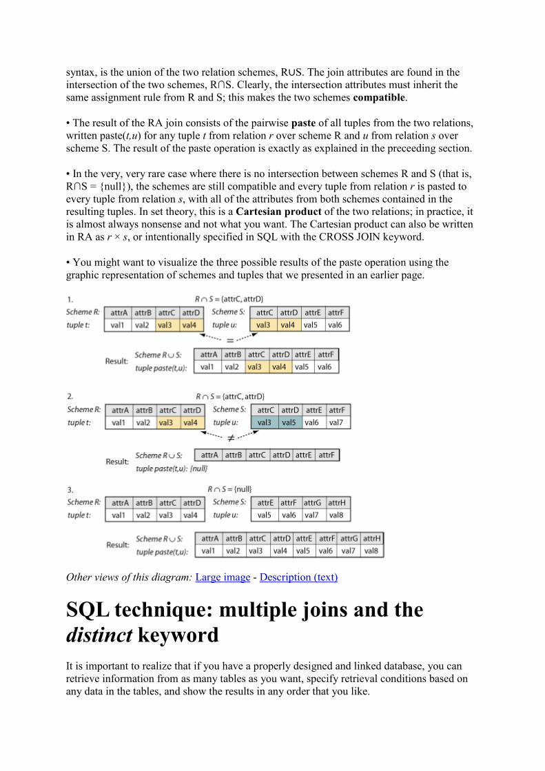
syntax, is the union of the two relation schemes, R∪S. The join attributes are found in the
intersection of the two schemes, R∩S. Clearly, the intersection attributes must inherit the
same assignment rule from R and S; this makes the two schemes compatible.
• The result of the RA join consists of the pairwise paste of all tuples from the two relations,
written paste(t,u) for any tuple t from relation r over scheme R and u from relation s over
scheme S. The result of the paste operation is exactly as explained in the preceeding section.
• In the very, very rare case where there is no intersection between schemes R and S (that is,
R∩S = {null}), the schemes are still compatible and every tuple from relation r is pasted to
every tuple from relation s, with all of the attributes from both schemes contained in the
resulting tuples. In set theory, this is a Cartesian product of the two relations; in practice, it
is almost always nonsense and not what you want. The Cartesian product can also be written
in RA as r × s, or intentionally specified in SQL with the CROSS JOIN keyword.
• You might want to visualize the three possible results of the paste operation using the
graphic representation of schemes and tuples that we presented in an earlier page.
Other views of this diagram: Large image - Description (text)
SQL technique: multiple joins and the
distinct keyword
It is important to realize that if you have a properly designed and linked database, you can
retrieve information from as many tables as you want, specify retrieval conditions based on
any data in the tables, and show the results in any order that you like.

Example: We’ll use the order entry model. We’d like a list of all the products that have been
purchased by a specific customer.
• Unless you can memorize the exact spelling of every attribute in the database, along with all
the PKs and FKs (I can’t), you should keep a copy of the relation scheme diagram handy
when you build the query. We’ll show it again here, circling the attributes that we need for
this query.
Other views of this diagram: Large image - Description (text)
• Our query is still a simple one that could be expressed in RA using only the select, project,
and join operators:
πcLastName, cFirstName, prodName σcFirstName='Alvaro' and cLastName='Monge'
(customers orders orderlines products)
• The information that we need is found in the Products table. You could think of this as
“output” from the query that will be part of the SELECT clause attribute list. The retrieval
condition, or “input” to the query, is based on the Customers table—these attributes will be
needed for the WHERE clause. You should include these attributes in the SELECT list, so
that you are sure that your query is showing the data that you want.
• We will also need to include the intervening tables in the FROM clause of the query, since
this is the only way to correctly associate the Customers data with the Products data. (You
can’t join Customers to Products, because they don’t have any common attributes.)
• Another way to think about this is to simply “follow the PK-FK pairs” from table to table
until you have completely linked all of the information you need. If you look carefully at the
relation scheme for this query, you will realize that we could have bypassed the Orders table
(since the custID is also part of the OrderLines scheme). If there were an orderID, or if we
needed data from the Orders table, it would have to be included, so we’ll keep it here for

illustration. In SQL, we’ll build the query using the same step-by-step procedure that you
have seen before.
1. Look at the result set (all of the linked data). We won’t show the result here because of
space limitations on the web page.
SELECT *
FROM customers
NATURAL JOIN orders
NATURAL JOIN orderlines
NATURAL JOIN products;
• Your database system might not support the NATURAL JOIN syntax that we show here.
We’ll discuss this issue further when we look at join types. The multiple natural joins in our
example work correctly because there are no non-pk/fk attributes in any of our tables that
have the same name. In larger, more complicated databases, this might not be true.
2. Pick the rows you want, and be sure that all of the information makes sense and is really
what you are looking for. (This one is still too wide for the page.)
SELECT *
FROM customers
NATURAL JOIN orders
NATURAL JOIN orderlines
NATURAL JOIN products
WHERE cFirstName = 'Alvaro' AND cLastName = 'Monge';
3. Now pick the columns that you want, and again check the results. Notice that we are
including the retreival condition attributes in the SELECT clause, to be sure that this really is
the right answer.
SELECT cFirstName, cLastName, prodName
FROM customers
NATURAL JOIN orders
NATURAL JOIN orderlines
NATURAL JOIN products
WHERE cFirstName = 'Alvaro' AND cLastName = 'Monge';
Products purchased
cFirst,ame cLast,ame prod,ame
Alvaro Monge Hammer, framing, 20 oz.
Alvaro Monge Hammer, framing, 20 oz.
Alvaro Monge Screwdriver, Phillips #2, 6 inch
Alvaro Monge Screwdriver, Phillips #2, 6 inch
Alvaro Monge Pliers, needle-nose, 4 inch
The distinct keyword
Oops! We only wanted a list of the individual product names that this customer has
purchased, but some of them are listed more than once. What went wrong?
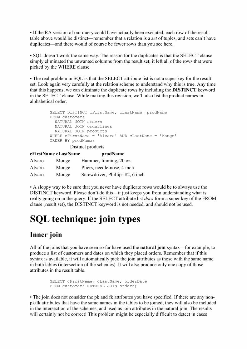
• If the RA version of our query could have actually been executed, each row of the result
table above would be distinct—remember that a relation is a set of tuples, and sets can’t have
duplicates—and there would of course be fewer rows than you see here.
• SQL doesn’t work the same way. The reason for the duplicates is that the SELECT clause
simply eliminated the unwanted columns from the result set; it left all of the rows that were
picked by the WHERE clause.
• The real problem in SQL is that the SELECT attribute list is not a super key for the result
set. Look again very carefully at the relation scheme to understand why this is true. Any time
that this happens, we can eliminate the duplicate rows by including the DISTI,CT keyword
in the SELECT clause. While making this revision, we’ll also list the product names in
alphabetical order.
SELECT DISTINCT cFirstName, cLastName, prodName
FROM customers
NATURAL JOIN orders
NATURAL JOIN orderlines
NATURAL JOIN products
WHERE cFirstName = 'Alvaro' AND cLastName = 'Monge'
ORDER BY prodName;
Distinct products
cFirst,ame cLast,ame prod,ame
Alvaro Monge Hammer, framing, 20 oz.
Alvaro Monge Pliers, needle-nose, 4 inch
Alvaro Monge Screwdriver, Phillips #2, 6 inch
• A sloppy way to be sure that you never have duplicate rows would be to always use the
DISTINCT keyword. Please don’t do this—it just keeps you from understanding what is
really going on in the query. If the SELECT attribute list does form a super key of the FROM
clause (result set), the DISTINCT keyword is not needed, and should not be used.
SQL technique: join types
Inner join
All of the joins that you have seen so far have used the natural join syntax—for example, to
produce a list of customers and dates on which they placed orders. Remember that if this
syntax is available, it will automatically pick the join attributes as those with the same name
in both tables (intersection of the schemes). It will also produce only one copy of those
attributes in the result table.
SELECT cFirstName, cLastName, orderDate
FROM customers NATURAL JOIN orders;
• The join does not consider the pk and fk attributes you have specified. If there are any non-
pk/fk attributes that have the same names in the tables to be joined, they will also be included
in the intersection of the schemes, and used as join attributes in the natural join. The results
will certainly not be correct! This problem might be especially difficult to detect in cases

where many natural joins are performed in the same query. Fortunately, you can always
specify the join attributes yourself, as we describe next.
• Another keyword that produces the same results (without the potential attribute name
problem) is the inner join. With this syntax, you may specify the join attributes in a USING
clause. (Multiple join attributes in the USING clause are separated by commas.) This also
produces only one copy of the join attributes in the result table. Like the NATURAL JOIN
syntax, the USING clause is not supported by all systems.
SELECT cFirstName, cLastName, orderDate
FROM customers INNER JOIN orders
USING (custID);
• The most widely-used (and most portable) syntax for the inner join substitutes an ON clause
for the USING clause. This requires you to explicitly specify not only the join attribute
names, but the join condition (normally equality). It also requires you to preface (qualify) the
join attribute names with their table name, since both columns will be included in the result
table. This is the only syntax that will let you use join attributes that have different names in
the tables to be joined. Unfortunately, it also allows you to join tables on attributes other than
the pk/fk pairs, which was a pre-1992 way to answer queries that can be written in better
ways today.
SELECT cFirstName, cLastName, orderDate
FROM customers INNER JOIN orders
ON customers.custID = orders.custID;
• You can save a bit of typing by specifying an alias for each table name (such as c and o in
this example), then using the alias instead of the full name when you refer to the attributes.
This is the only syntax that will let you join a table to itself, as we will see when we discuss
recursive relationships.
SELECT cFirstName, cLastName, orderDate
FROM customers c INNER JOIN orders o
ON c.custID = o.custID;
• All of the join statements above are specified as part of the 1992 SQL standard, which was
not widely supported for several years after that. In earlier systems, joins were done with the
1986 standard SQL syntax. Although you shouldn’t use this unless you absolutely have to,
you just might get stuck working on an older database. If so, you should recognize that the
join condition is placed confusingly in the WHERE clause, along with all of the tests to pick
the right rows:
SELECT cFirstName, cLastName, orderDate
FROM customers c, orders o
WHERE c.custID = o.custID;
Outer join
One important effect of all natural and inner joins is that any unmatched PK value simply
drops out of the result. In our example, this means that any customer who didn’t place an
order isn’t shown. Suppose that we want a list of all customers, along with order date(s) for

those who did place orders. To include the customers who did not place orders, we will use
an outer join, which may take either the USING or the ON clause syntax.
SELECT cFirstName, cLastName, orderDate
FROM customers c LEFT OUTER JOIN orders o
ON c.custID = o.custID;
All customers and order dates
cfirstname clastname orderdate
Tom Jewett
Alvaro Monge 2003-07-14
Alvaro Monge 2003-07-18
Alvaro Monge 2003-07-20
Wayne Dick 2003-07-14
• Notice that for customers who placed no orders, any attributes from the Orders table are
simply filled with NULL values.
• The word “left” refers to the order of the tables in the FROM clause (customers on the left,
orders on the right). The left table here is the one that might have unmatched join attributes—
the one from which we want all rows. We could have gotten exactly the same results if the
table names and outer join direction were reversed:
SELECT cFirstName, cLastName, orderDate
FROM orders o RIGHT OUTER JOIN customers c
ON o.custID = c.custID;
• An outer join makes sense only if one side of the relationship has a minimum cardinality of
zero (as Orders does in this example). Otherwise, the outer join will produce exactly the same
result as an inner join (for example, between Orders and OrderLines).
• The SQL standard also allows a FULL outer join, in which unmatched join attributes from
either side are paired with null values on the other side. You will probably not have to use
this with most well-designed databases.
Evaluation order
Multiple joins in a query are evaluated left-to-right in the order that you write them, unless
you use parentheses to force a different evaluation order. (Some database systems require
parentheses in any case.) The schemes of the joins are also cumulative in the order that they
are evaluated; in RA, this means that
r1 r2 r3 = (r1 r2) r3.
• It is especially important to remember this rule when outer joins are mixed with other joins
in a query. For example, if you write:
SELECT cFirstName, cLastName, orderDate, UPC, quantity
FROM customers LEFT OUTER JOIN orders USING (custID)
NATURAL JOIN orderlines;

you will lose the customers who haven’t placed orders. They will be retained if you force the
second join to be executed first:
SELECT cFirstName, cLastName, orderDate, UPC, quantity
FROM customers LEFT OUTER JOIN
(orders NATURAL JOIN orderlines)
USING (custID);
Other join types
For sake of completeness, you should also know that if you try to join two tables with no join
condition, the result will be that every row from one side is paired with every row from the
other side. Mathematically, this is a Cartesian product of the two tables, as you have seen
before. It is almost never what you want. In pre-1992 syntax, it is easy to do this accidently,
by forgetting to put the join condition in the WHERE clause:
SELECT cFirstName, cLastName, orderDate
FROM customers, orders;
• If your system is backward-compatible (most are), you might actually try this just to prove
to yourself that the result is pure nonsense. However, if you ever have an occasion to really
need a Cartesian product of two tables, use the new cross join syntax to prove that you really
mean it. Notice that this example still produces nonsense.
SELECT cFirstName, cLastName, orderDate
FROM customers CROSS JOIN orders;
• It is possible, but confusing, to specify a join condition other than equality of two attributes;
this is called a non-equi-join. If you see such a thing in older code, it probably represents a
WHERE clause or subquery in disguise.
• You may also hear the term self join, which is nothing but an inner or outer join between
two attributes in the same table. We’ll look at these when we discuss recursive relationships.
SQL technique: functions
Sometimes, the information that we need is not actually stored in the database, but has to be
computed in some way from the stored data. In our order entry example, there are two
derived attributes (/subtotal in OrderLines and /total in Orders) that are part of the class
diagram but not part of the relation scheme. We can compute these by using SQL functions in
the SELECT statement.
There are many, many functions in any implementation of SQL—far more than we can show
here. Unfortunately, many of the functions are defined quite differently in different database
packages, so you should always consult a reference manual for your specific software.
Computed columns
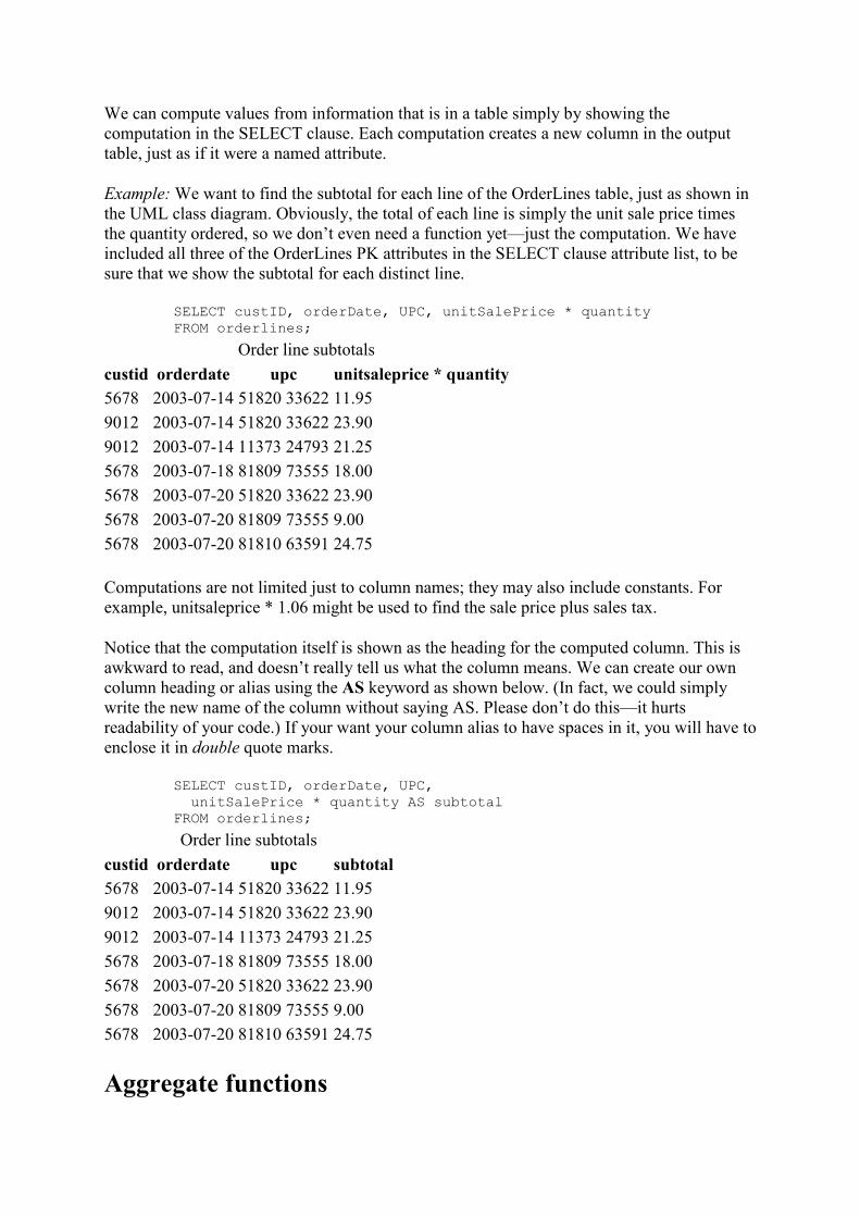
We can compute values from information that is in a table simply by showing the
computation in the SELECT clause. Each computation creates a new column in the output
table, just as if it were a named attribute.
Example: We want to find the subtotal for each line of the OrderLines table, just as shown in
the UML class diagram. Obviously, the total of each line is simply the unit sale price times
the quantity ordered, so we don’t even need a function yet—just the computation. We have
included all three of the OrderLines PK attributes in the SELECT clause attribute list, to be
sure that we show the subtotal for each distinct line.
SELECT custID, orderDate, UPC, unitSalePrice * quantity
FROM orderlines;
Order line subtotals
custid orderdate upc unitsaleprice * quantity
5678 2003-07-14 51820 33622 11.95
9012 2003-07-14 51820 33622 23.90
9012 2003-07-14 11373 24793 21.25
5678 2003-07-18 81809 73555 18.00
5678 2003-07-20 51820 33622 23.90
5678 2003-07-20 81809 73555 9.00
5678 2003-07-20 81810 63591 24.75
Computations are not limited just to column names; they may also include constants. For
example, unitsaleprice * 1.06 might be used to find the sale price plus sales tax.
Notice that the computation itself is shown as the heading for the computed column. This is
awkward to read, and doesn’t really tell us what the column means. We can create our own
column heading or alias using the AS keyword as shown below. (In fact, we could simply
write the new name of the column without saying AS. Please don’t do this—it hurts
readability of your code.) If your want your column alias to have spaces in it, you will have to
enclose it in double quote marks.
SELECT custID, orderDate, UPC,
unitSalePrice * quantity AS subtotal
FROM orderlines;
Order line subtotals
custid orderdate upc subtotal
5678 2003-07-14 51820 33622 11.95
9012 2003-07-14 51820 33622 23.90
9012 2003-07-14 11373 24793 21.25
5678 2003-07-18 81809 73555 18.00
5678 2003-07-20 51820 33622 23.90
5678 2003-07-20 81809 73555 9.00
5678 2003-07-20 81810 63591 24.75
Aggregate functions
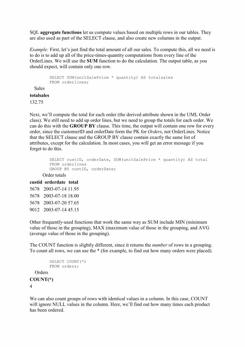
SQL aggregate functions let us compute values based on multiple rows in our tables. They
are also used as part of the SELECT clause, and also create new columns in the output.
Example: First, let’s just find the total amount of all our sales. To compute this, all we need is
to do is to add up all of the price-times-quantity computations from every line of the
OrderLines. We will use the SUM function to do the calculation. The output table, as you
should expect, will contain only one row.
SELECT SUM(unitSalePrice * quantity) AS totalsales
FROM orderlines;
Sales
totalsales
132.75
Next, we’ll compute the total for each order (the derived attribute shown in the UML Order
class). We still need to add up order lines, but we need to group the totals for each order. We
can do this with the GROUP BY clause. This time, the output will contain one row for every
order, since the customerID and orderDate form the PK for Orders, not OrderLines. Notice
that the SELECT clause and the GROUP BY clause contain exactly the same list of
attributes, except for the calculation. In most cases, you will get an error message if you
forget to do this.
SELECT custID, orderDate, SUM(unitSalePrice * quantity) AS total
FROM orderlines
GROUP BY custID, orderDate;
Order totals
custid orderdate total
5678 2003-07-14 11.95
5678 2003-07-18 18.00
5678 2003-07-20 57.65
9012 2003-07-14 45.15
Other frequently-used functions that work the same way as SUM include MIN (minimum
value of those in the grouping), MAX (maximum value of those in the grouping, and AVG
(average value of those in the grouping).
The COUNT function is slightly different, since it returns the number of rows in a grouping.
To count all rows, we can use the * (for example, to find out how many orders were placed).
SELECT COUNT(*)
FROM orders;
Orders
COU,T(*)
4
We can also count groups of rows with identical values in a column. In this case, COUNT
will ignore NULL values in the column. Here, we’ll find out how many times each product
has been ordered.
SELECT prodname AS "product name",
COUNT(prodname) AS "times ordered"
FROM products NATURAL JOIN orderlines
GROUP BY prodname;
Product orders
product name times ordered
Hammer, framing, 20 oz. 3
Pliers, needle-nose, 4 inch 1
Saw, crosscut, 10 tpi 1
Screwdriver, Phillips #2, 6 inch 2
A WHERE clause can be used as usual before the GROUP BY, to eliminate rows before the
group function is executed. However, if we want to select output rows based on the results of
the group function, the HAVI,G clause is used instead. For example, we could ask for only
those products that have been sold more than once:
SELECT prodname AS "product name",
COUNT(prodname) AS "times ordered"
FROM products NATURAL JOIN orderlines
GROUP BY prodname
HAVING COUNT(prodname) > 1;
Other functions
Most database systems offer a wide variety of functions that deal with formatting and other
miscellaneous tasks. These functions tend to be proprietary, differing widely from system to
system in both availability and syntax. Most are used in the SELECT clause, although some
might appear in a WHERE clause expression or an INSERT or UPDATE statement. Typical
functions include:
• Functions for rounding, truncating, converting, and formatting numeric data types.
• Functions for concatenating, altering case, and manipulating character data types.
• Functions for formatting dates and times, or retrieving the date and time from the operating
system.
• Functions for converting data types such as date or numeric to character string, and vice-
versa.
• Functions for supplying visible values to null attributes, allowing conditional output, and
other miscellaneous tasks.
SQL technique: subqueries
Sometimes you don’t have enough information available when you design a query to
determine which rows you want. In this case, you’ll have to find the required information
with a subquery.

Example: Find the name of customers who live in the same zip code area as Wayne Dick. We
might start writing this query as we would any of the ones that we have already done:
SELECT cFirstName, cLastName
FROM customers
WHERE cZipCode = ???
• Oops! We don’t know what zip code to put in the WHERE clause. No, we can’t look it up
manually and type it into the query—we have to find the answer based only on the
information that we have been given!
• Fortunately, we also know how to find the right zip code by writing another query:
SELECT cZipCode
FROM Customers
WHERE cFirstName = 'Wayne' AND cLastName = 'Dick';
Zip code
czipcode
90840
• Notice that this query returns a single column and a single row. We can use the result as the
condition value for cZipCode in our original query. In effect, the output of the second query
becomes input to the first one, which we can illustrate with their relation schemes:
• Syntactically, all we have to do is to enclose the subquery in parenthses, in the same place
where we would normally use a constant in the WHERE clause. We’ll include the zip code in
the SELECT line to verify that the answer is what we want:
SELECT cFirstName, cLastName, cZipCode
FROM customers
WHERE cZipCode =
(SELECT cZipCode
FROM customers
WHERE cFirstName = 'Wayne' AND cLastName = 'Dick');
Customers
cfirstname clastname czipcode
Alvaro Monge 90840
Wayne Dick 90840
A subquery that returns only one column and one row can be used any time that we need a
single value. Another example would be to find the product name and sale price of all
products whose unit sale price is greater than the average of all products. We can see that the
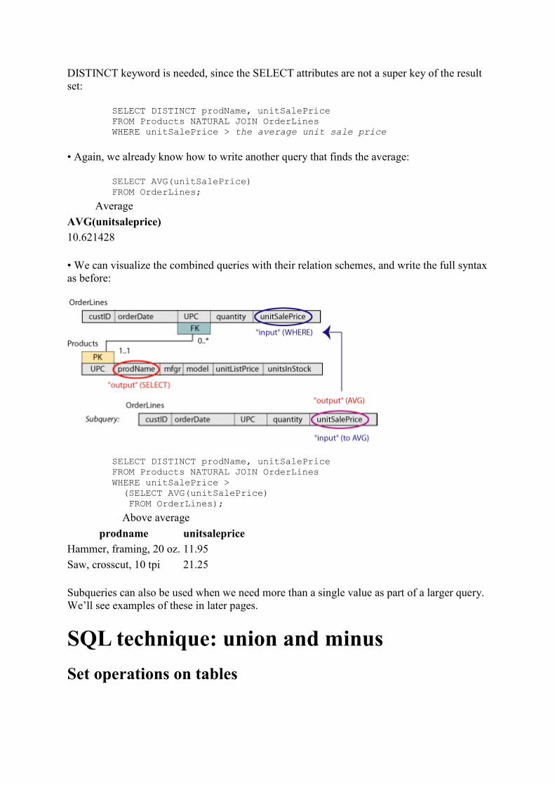
DISTINCT keyword is needed, since the SELECT attributes are not a super key of the result
set:
SELECT DISTINCT prodName, unitSalePrice
FROM Products NATURAL JOIN OrderLines
WHERE unitSalePrice > the average unit sale price
• Again, we already know how to write another query that finds the average:
SELECT AVG(unitSalePrice)
FROM OrderLines;
Average
AVG(unitsaleprice)
10.621428
• We can visualize the combined queries with their relation schemes, and write the full syntax
as before:
SELECT DISTINCT prodName, unitSalePrice
FROM Products NATURAL JOIN OrderLines
WHERE unitSalePrice >
(SELECT AVG(unitSalePrice)
FROM OrderLines);
Above average
prodname unitsaleprice
Hammer, framing, 20 oz. 11.95
Saw, crosscut, 10 tpi 21.25
Subqueries can also be used when we need more than a single value as part of a larger query.
We’ll see examples of these in later pages.
SQL technique: union and minus
Set operations on tables
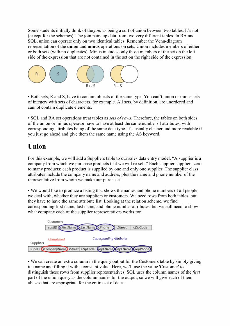
Some students initially think of the join as being a sort of union between two tables. It’s not
(except for the schemes). The join pairs up data from two very different tables. In RA and
SQL, union can operate only on two identical tables. Remember the Venn-diagram
representation of the union and minus operations on sets. Union includes members of either
or both sets (with no duplicates). Minus includes only those members of the set on the left
side of the expression that are not contained in the set on the right side of the expression.
• Both sets, R and S, have to contain objects of the same type. You can’t union or minus sets
of integers with sets of characters, for example. All sets, by definition, are unordered and
cannot contain duplicate elements.
• SQL and RA set operations treat tables as sets of rows. Therefore, the tables on both sides
of the union or minus operator have to have at least the same number of attributes, with
corresponding attributes being of the same data type. It’s usually cleaner and more readable if
you just go ahead and give them the same name using the AS keyword.
Union
For this example, we will add a Suppliers table to our sales data entry model. “A supplier is a
company from which we purchase products that we will re-sell.” Each supplier suppliers zero
to many products; each product is supplied by one and only one supplier. The supplier class
attributes include the company name and address, plus the name and phone number of the
representative from whom we make our purchases.
• We would like to produce a listing that shows the names and phone numbers of all people
we deal with, whether they are suppliers or customers. We need rows from both tables, but
they have to have the same attribute list. Looking at the relation scheme, we find
corresponding first name, last name, and phone number attributes, but we still need to show
what company each of the supplier representatives works for.
• We can create an extra column in the query output for the Customers table by simply giving
it a name and filling it with a constant value. Here, we’ll use the value 'Customer' to
distinguish these rows from supplier representatives. SQL uses the column names of the first
part of the union query as the column names for the output, so we will give each of them
aliases that are appropriate for the entire set of data.

• Build and test each component of the union query individually, then put them together. The
ORDER BY clause has to come at the end.
SELECT cLastName AS "Last Name", cFirstName AS "First Name",
cPhone as "Phone", 'Customer' AS "Company"
FROM customers
UNION
SELECT repLName, repFName, repPhone, sCompanyName
FROM suppliers
ORDER BY "Last Name";
Phone list
Last ,ame First ,ame Phone Company
Bradley Jerry 888-736-8000 Industrial Tool Supply
Dick Wayne 562-777-3030 Customer
Jewett Tom 714-555-1212 Customer
Monge Alvaro 562-333-4141 Customer
O'Brien Tom 949-567-2312 Bosch Machine Tools
Minus
Sometimes you have to think about both what you do want and what you don’t want in the
results of a query. If there is a WHERE clause predicate that completely partitions all rows of
interest (the result set) into those you want and those you don’t want, then you have a simple
query with a test for inequality.
• The multiplicity of an association can help you determine how to build the query. Since
each product has one and only one supplier, we can partition the Products table into those that
are supplied by a given company and those that are not.
SELECT prodName, sCompanyName
FROM Products NATURAL JOIN Suppliers
WHERE sCompanyName <> 'Industrial Tool Supply';
• Contrast this to finding customers who did not make purchases in 2002. Because of the
optional one-to-many association between Customers and Orders, there are actually four
possibilities:
1. A customer made purchases in 2002 (only).
2. A customer made purchases in other years, but not in 2002.
3. A customer made purchases both in other years and in 2002.
4. A customer made no purchases in any year.
• If you try to write this as a simple test for inequality,
SELECT DISTINCT cLastName, cFirstName, cStreet, cZipCode
FROM Customers NATURAL JOIN Orders
WHERE TO_CHAR(orderDate, 'YYYY') <> '2002';

you will correctly exclude group 1 and include group 2, but falsely include group 3 and
falsely exclude group 4. Please take time to re-read this statement and convince yourself why
it is true!
• We can show in set notation what we need to do:
{customers who did not make purchases in 2002} =
{all customers} − {those who did}
There are two ways to write this in SQL.
• The easiest syntax in this case is to compare only the customer IDs. We’ll use the NOT IN
set operator in the WHERE clause, along with a subquery to find the customer ID of those
who did made purchases in 2002.
SELECT cLastName, cFirstName, cStreet, cZipCode
FROM Customers
WHERE custID NOT IN
(SELECT custID
FROM Orders
WHERE TO_CHAR(orderDate, 'YYYY') = '2002');
• We can also use the MINUS operator to subtract rows we don’t want from all rows in
Customers. (Some versions of SQL use the keyword EXCEPT instead of MINUS.) Like the
UNION, this requires the schemes of the two tables to match exactly in number and type of
attributes.
SELECT cLastName, cFirstName, cStreet, cZipCode
FROM Customers
MINUS
SELECT cLastName, cFirstName, cStreet, cZipCode
FROM Customers NATURAL JOIN Orders
WHERE TO_CHAR(orderDate, 'YYYY') = '2002';
Other set operations
SQL has two additional set operators. UNION ALL works like UNION, except it keeps
duplicate rows in the result. INTERSECT operates just like you would expect from set
theory; again, the schemes of the two tables must match exactly.
SQL technique: views and indexes
A view is simply any SELECT query that has been given a name and saved in the database.
For this reason, a view is sometimes called a named query or a stored query. To create a
view, you use the SQL syntax:
CREATE OR REPLACE VIEW <view_name> AS
SELECT <any valid select query>;
• The view query itself is saved in the database, but it is not actually run until it is called with
another SELECT statement. For this reason, the view does not take up any disk space for data

storage, and it does not create any redundant copies of data that is already stored in the tables
that it references (which are sometimes called the base tables of the view).
• Although it is not required, many database developers identify views with names such as
v_Customers or Customers_view. This not only avoids name conflicts with base tables, it
helps in reading any query that uses a view.
• The keywords OR REPLACE in the syntax shown above are optional. Although you don’t
need to use them the first time that you create a view, including them will overwrite an older
version of the view with your latest one, without giving you an error message.
• The syntax to remove a view from your schema is exactly what you would expect:
DROP VIEW <view_name>;
Using views
A view name may be used in exactly the same way as a table name in any SELECT query.
Once stored, the view can be used again and again, rather than re-writing the same query
many times.
• The most basic use of a view would be to simply SELECT * from it, but it also might
represent a pre-written subquery or a simplified way to write part of a FROM clause.
• In many systems, views are stored in a pre-compiled form. This might save some execution
time for the query, but usually not enough for a human user to notice.
• One of the most important uses of views is in large multi-user systems, where they make it
easy to control access to data for different types of users. As a very simple example, suppose
that you have a table of employee information on the scheme Employees = {employeeID,
empFName, empLName, empPhone, jobTitle, payRate, managerID}. Obviously, you can’t
let everyone in the company look at all of this information, let alone make changes to it.
• Your database administrator (DBA) can define roles to represent different groups of users,
and then grant membership in one or more roles to any specific user account (schema). In
turn, you can grant table-level or view-level permissions to a role as well as to a specific user.
Suppose that the DBA has created the roles managers and payroll for people who occupy
those positions. In Oracle®, there is also a pre-defined role named public, which means every
user of the database.
• You could create separate views even on just the Employees table, and control access to
them like this:
CREATE VIEW phone_view AS
SELECT empFName, empLName, empPhone FROM Employees;
GRANT SELECT ON phone_view TO public;
CREATE VIEW job_view AS
SELECT employeeID, empFName, empLName, jobTitle, managerID FROM
Employees;
GRANT SELECT, UPDATE ON job_view TO managers;

CREATE VIEW pay_view AS
SELECT employeeID, empFName, empLName, payRate FROM Employees;
GRANT SELECT, UPDATE ON pay_view TO payroll;
• Only a very few trusted people would have SELECT, UPDATE, INSERT, and DELETE
privileges on the entire Employees base table; everyone else would now have exactly the
access that they need, but no more.
• When a view is the target of an UPDATE statement, the base table value is changed. You
can’t change a computed value in a view, or any value in a view that is based on a UNION
query. You may also use a view as the target of an INSERT or DELETE statement, subject to
any integrity constraints that have been placed on the base tables.
Materialized views
Sometimes, the execution speed of a query is so important that a developer is willing to trade
increased disk space use for faster response, by creating a materialized view. Unlike the
view discussed above, a materialized view does create and store the result table in advance,
filled with data. The scheme of this table is given by the SELECT clause of the view
definition.
• This technique is most useful when the query involves many joins of large tables, or any
other SQL feature that could contribute to long execution times. You might encounter this in
a Web project, where the site visitor simply can’t be kept waiting while the query runs.
• Since the view would be useless if it is out of date, it must be re-run, at the minimum, when
there is a change to any of the tables that it is based on. The SQL syntax to create a
materialized view includes many options for when it is first to be run, how often it is to be re-
run, and so on. This requires an advanced reference manual for your specific system, and is
beyond the scope of this tutorial.
Indexes
An index, as you would expect, is a data structure that the database uses to find records
within a table more quickly. Indexes are built on one or more columns of a table; each index
maintains a list of values within that field that are sorted in ascending or descending order.
Rather than sorting records on the field or fields during query execution, the system can
simply access the rows in order of the index.
Unique and non-unique indexes: When you create an index, you may allow the indexed
columns to contain duplicate values; the index will still list all of the rows with duplicates.
You may also specify that values in the indexed columns must be unique, just as they must be
with a primary key. In fact, when you create a primary key constraint on a table, Oracle and
most other systems will automatically create a unique index on the primary key columns, as
well as not allowing null values in those columns. One good reason for you to create a unique
index on non-primary key fields is to enforce the integrity of a candidate key, which
otherwise might end up having (nonsense) duplicate values in different rows.

Queries versus insertion/update: It might seem as if you should create an index on every
column or group of columns that will ever by used in an ORDER BY clause (for example:
lastName, firstName). However, each index will have to be updated every time that a row is
inserted or a value in that column is updated. Although index structures such as B or B+ trees
allow this to happen very quickly, there still might be circumstances where too many indexes
would detract from overall system performance. This and similar issues are often covered in
more advanced courses.
Syntax: As you would expect by now, the SQL to create an index is:
CREATE INDEX <indexname> ON <tablename> (<column>, <column>...);
To enforce unique values, add the UNIQUE keyword:
CREATE UNIQUE INDEX <indexname> ON <tablename> (<column>,
<column>...);
To specify sort order, add the keyword ASC or DESC after each column name, just as you
would do in an ORDER BY clause.
To remove an index, simply enter:
DROP INDEX <indexname>;
Glossary
[ Skip navigation ] Show: [ all keywords ] [ A–C ] [ D–H ] [ I–N ] [ O–R ] [ S–Z ]
Glossary
keyword definition page_link
aggregate function (SQL) Function that operates on a group of rows, for
example, SUM. functions.php
aggregation
(UML) An association in which one class represents an
assembly of components from one or more other class
types. Components may also exist without being part of
the assembly.
aggregate.php
alias (SQL) An alternate, short name for a table in the
FROM clause of a SELECT statement. jointypes.php
ALTER TABLE (SQL) Statement to change structure, constraints, or
other properties of a table. tables.php
AS (SQL) Keyword to specify a column alias in the
SELECT clause. functions.php
assignment rule (RM) The association of each attribute in a scheme with
its domain. class.php
association (UML) The way that two classes are functionally
connected to each other. association.php
association class (UML) A class that contains attributes which are the manymany.php
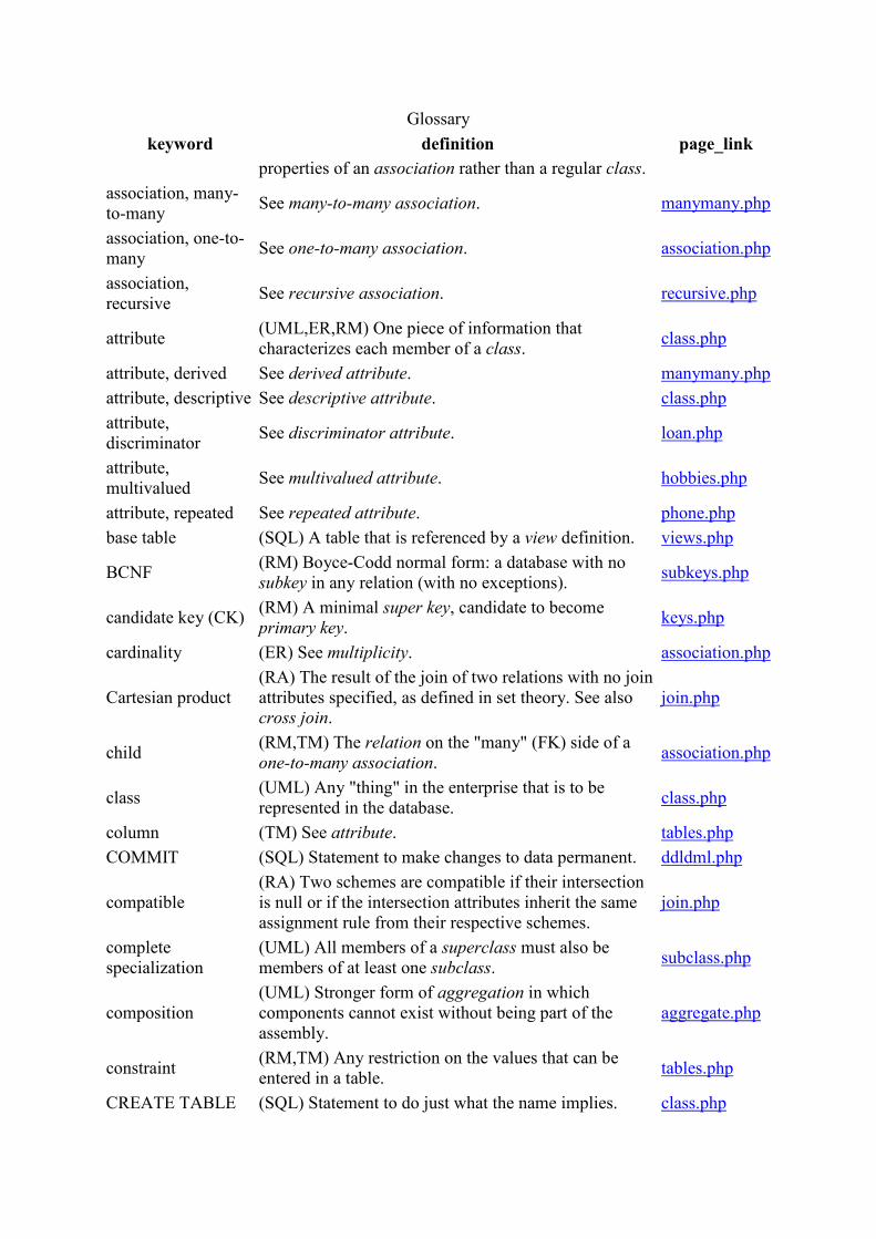
Glossary
keyword definition page_link
properties of an association rather than a regular class.
association, many-
to-many See many-to-many association. manymany.php
association, one-to-
many See one-to-many association. association.php
association,
recursive See recursive association. recursive.php
attribute (UML,ER,RM) One piece of information that
characterizes each member of a class. class.php
attribute, derived See derived attribute. manymany.php
attribute, descriptive See descriptive attribute. class.php
attribute,
discriminator See discriminator attribute. loan.php
attribute,
multivalued See multivalued attribute. hobbies.php
attribute, repeated See repeated attribute. phone.php
base table (SQL) A table that is referenced by a view definition. views.php
BCNF (RM) Boyce-Codd normal form: a database with no
subkey in any relation (with no exceptions). subkeys.php
candidate key (CK) (RM) A minimal super key, candidate to become
primary key. keys.php
cardinality (ER) See multiplicity. association.php
Cartesian product
(RA) The result of the join of two relations with no join
attributes specified, as defined in set theory. See also
cross join.
join.php
child (RM,TM) The relation on the "many" (FK) side of a
one-to-many association. association.php
class (UML) Any "thing" in the enterprise that is to be
represented in the database. class.php
column (TM) See attribute. tables.php
COMMIT (SQL) Statement to make changes to data permanent. ddldml.php
compatible
(RA) Two schemes are compatible if their intersection
is null or if the intersection attributes inherit the same
assignment rule from their respective schemes.
join.php
complete
specialization
(UML) All members of a superclass must also be
members of at least one subclass. subclass.php
composition
(UML) Stronger form of aggregation in which
components cannot exist without being part of the
assembly.
aggregate.php
constraint (RM,TM) Any restriction on the values that can be
entered in a table. tables.php
CREATE TABLE (SQL) Statement to do just what the name implies. class.php
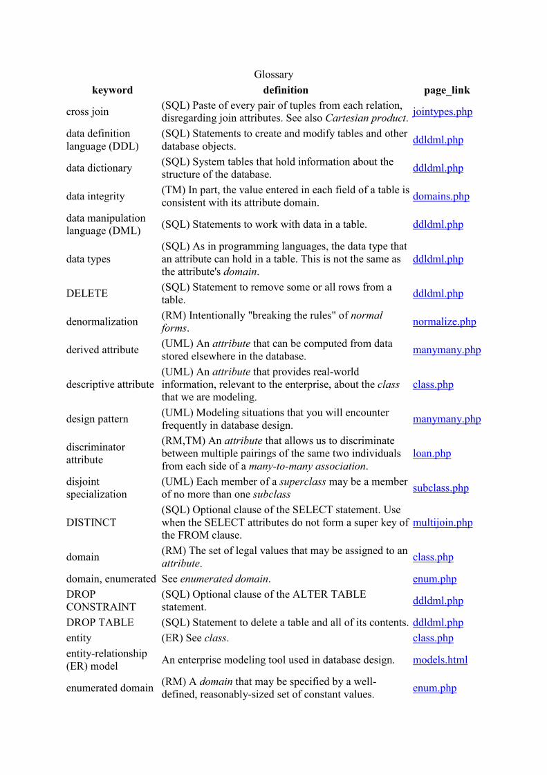
Glossary
keyword definition page_link
cross join (SQL) Paste of every pair of tuples from each relation,
disregarding join attributes. See also Cartesian product. jointypes.php
data definition
language (DDL)
(SQL) Statements to create and modify tables and other
database objects. ddldml.php
data dictionary (SQL) System tables that hold information about the
structure of the database. ddldml.php
data integrity (TM) In part, the value entered in each field of a table is
consistent with its attribute domain. domains.php
data manipulation
language (DML) (SQL) Statements to work with data in a table. ddldml.php
data types
(SQL) As in programming languages, the data type that
an attribute can hold in a table. This is not the same as
the attribute's domain.
ddldml.php
DELETE (SQL) Statement to remove some or all rows from a
table. ddldml.php
denormalization (RM) Intentionally "breaking the rules" of normal
forms. normalize.php
derived attribute (UML) An attribute that can be computed from data
stored elsewhere in the database. manymany.php
descriptive attribute
(UML) An attribute that provides real-world
information, relevant to the enterprise, about the class
that we are modeling.
class.php
design pattern (UML) Modeling situations that you will encounter
frequently in database design. manymany.php
discriminator
attribute
(RM,TM) An attribute that allows us to discriminate
between multiple pairings of the same two individuals
from each side of a many-to-many association.
loan.php
disjoint
specialization
(UML) Each member of a superclass may be a member
of no more than one subclass subclass.php
DISTINCT
(SQL) Optional clause of the SELECT statement. Use
when the SELECT attributes do not form a super key of
the FROM clause.
multijoin.php
domain (RM) The set of legal values that may be assigned to an
attribute. class.php
domain, enumerated See enumerated domain. enum.php
DROP
CONSTRAINT
(SQL) Optional clause of the ALTER TABLE
statement. ddldml.php
DROP TABLE (SQL) Statement to delete a table and all of its contents. ddldml.php
entity (ER) See class. class.php
entity-relationship
(ER) model An enterprise modeling tool used in database design. models.html
enumerated domain (RM) A domain that may be specified by a well-
defined, reasonably-sized set of constant values. enum.php
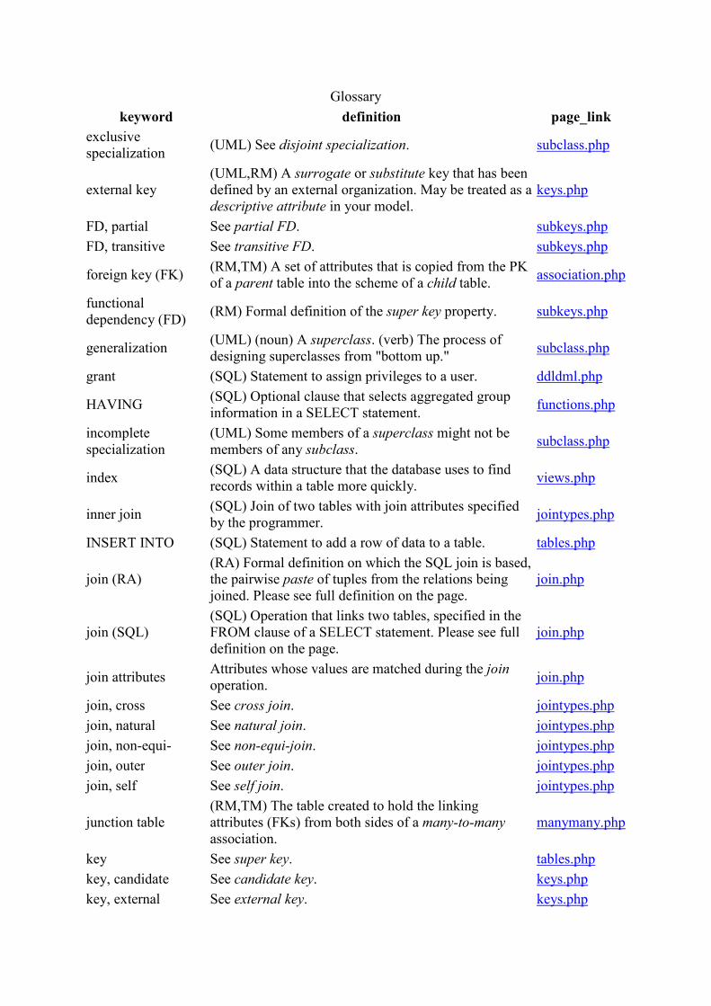
Glossary
keyword definition page_link
exclusive
specialization (UML) See disjoint specialization. subclass.php
external key
(UML,RM) A surrogate or substitute key that has been
defined by an external organization. May be treated as a
descriptive attribute in your model.
keys.php
FD, partial See partial FD. subkeys.php
FD, transitive See transitive FD. subkeys.php
foreign key (FK) (RM,TM) A set of attributes that is copied from the PK
of a parent table into the scheme of a child table. association.php
functional
dependency (FD) (RM) Formal definition of the super key property. subkeys.php
generalization (UML) (noun) A superclass. (verb) The process of
designing superclasses from "bottom up." subclass.php
grant (SQL) Statement to assign privileges to a user. ddldml.php
HAVING (SQL) Optional clause that selects aggregated group
information in a SELECT statement. functions.php
incomplete
specialization
(UML) Some members of a superclass might not be
members of any subclass. subclass.php
index (SQL) A data structure that the database uses to find
records within a table more quickly. views.php
inner join (SQL) Join of two tables with join attributes specified
by the programmer. jointypes.php
INSERT INTO (SQL) Statement to add a row of data to a table. tables.php
join (RA)
(RA) Formal definition on which the SQL join is based,
the pairwise paste of tuples from the relations being
joined. Please see full definition on the page.
join.php
join (SQL)
(SQL) Operation that links two tables, specified in the
FROM clause of a SELECT statement. Please see full
definition on the page.
join.php
join attributes Attributes whose values are matched during the join
operation. join.php
join, cross See cross join. jointypes.php
join, natural See natural join. jointypes.php
join, non-equi- See non-equi-join. jointypes.php
join, outer See outer join. jointypes.php
join, self See self join. jointypes.php
junction table
(RM,TM) The table created to hold the linking
attributes (FKs) from both sides of a many-to-many
association.
manymany.php
key See super key. tables.php
key, candidate See candidate key. keys.php
key, external See external key. keys.php

Glossary
keyword definition page_link
key, foreign See foreign key. association.php
key, primary See primary key. tables.php
key, sub See subkey. subkeys.php
key, substitute See substitute key. keys.php
key, super See super key. tables.php
key, surrogate See surrogate key. keys.php
lossless join
decomposition
Decomposition (breaking apart) of a relation scheme to
eliminate a subkey. The original scheme’s information
can be recreated with the join in a query.
subkeys.php
many-to-many
association
(UML) An association with maximum multiplicity of
*..* manymany.php
materialized view (SQL) A view that creates and stores a result table in
advance of being used. views.php
MINUS
(RA,SQL) Operation as defined in set theory, returning
the difference of the tuples/rows of two relations/tables
over the same scheme.
setops.php
multiplicity
(UML) The minimum and maximum number of
individuals of one class that may be associated with a
single member of another class.
association.php
multivalued attribute (UML) An attribute that contains more than one value
from its domain. This is a design error. hobbies.php
named query (SQL) A view. views.php
natural join (SQL) Join of two tables with the intersection of their
schemes used as join attributes. jointypes.php
non-equi-join (SQL) Join based on some condition other than equality
of the join attributes. jointypes.php
normal form, third See third normal form. subkeys.php
normal forms (RM) A progression of rules for well-structured
database design. normalize.php
normalization (RM) Following a set of rules to insure that a database
is well designed. See also normal forms. subkeys.php
NULL
(SQL) A special constant value, compatible with any
data type, that means "this field doesn't have any value
assigned to it."
phone.php
object (UML) The instantiation of a class in OO programming
languages. class.php
one-to-many
association
(UML) An association with maximum multiplicity of
1..* association.php
outer join (SQL) Join of two tables that retains unmatched join
attributes from one or both sides. jointypes.php
overlapping
specialization
(UML) Any member of a superclass may be a member
of more than one subclass. subclass.php
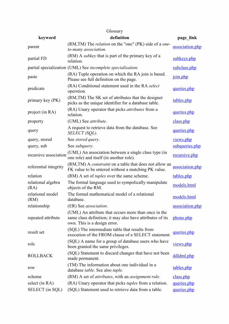
Glossary
keyword definition page_link
parent (RM,TM) The relation on the "one" (PK) side of a one-
to-many association. association.php
partial FD (RM) A subkey that is part of the primary key of a
relation. subkeys.php
partial specialization (UML) See incomplete specialization. subclass.php
paste (RA) Tuple operation on which the RA join is based.
Please see full definition on the page. join.php
predicate (RA) Conditional statement used in the RA select
operstion. queries.php
primary key (PK) (RM,TM) The SK set of attributes that the designer
picks as the unique identifier for a database table. tables.php
project (in RA) (RA) Unary operator that picks attributes from a
relation. queries.php
property (UML) See attribute. class.php
query A request to retrieve data from the database. See
SELECT (SQL). queries.php
query, stored See stored query. views.php
query, sub See subquery. subqueries.php
recursive association (UML) An association between a single class type (in
one role) and itself (in another role). recursive.php
referential integrity (RM,TM) A constraint on a table that does not allow an
FK value to be entered without a matching PK value. association.php
relation (RM) A set of tuples over the same scheme. tables.php
relational algebra
(RA)
The formal language used to sympolically manipulate
objects of the RM. models.html
relational model
(RM)
The formal mathematical model of a relational
database. models.html
relationship (ER) See association. association.php
repeated attribute
(UML) An attribute that occurs more than once in the
same class definition; it may also have attributes of its
own. This is a design error.
phone.php
result set (SQL) The intermediate table that results from
execution of the FROM clause of a SELECT statement. queries.php
role (SQL) A name for a group of database users who have
been granted the same privileges. views.php
ROLLBACK (SQL) Statement to discard changes that have not been
made permanent. ddldml.php
row (TM) The information about one individual in a
database table. See also tuple. tables.php
scheme (RM) A set of attributes, with an assignment rule. class.php
select (in RA) (RA) Unary operator that picks tuples from a relation. queries.php
SELECT (in SQL) (SQL) Statement used to retrieve data from a table. queries.php

Glossary
keyword definition page_link
self join (SQL) Join of one table to itself. jointypes.php
specialization (UML) (noun) A subclass. (verb) The process of
designing subclasses from "top down." subclass.php
specialization
constraints
(UML) Description of subclass membership
(incomplete versus complete, disjoint versus
overlapping).
subclass.php
specialization,
complete See complete specialization. subclass.php
specialization,
disjoint See disjoint specialization. subclass.php
specialization,
exclusive See disjoint specialization. subclass.php
specialization,
incomplete See incomplete specialization. subclass.php
specialization,
overlapping See overlapping specialization. subclass.php
specialization,
partial See incomplete specialization. subclass.php
stereotype (UML) A designator before a class name that specifies
the type of the class. enum.php
stored query (SQL) A view. views.php
structured query
language (SQL)
The language used to build and manipulate relational
databases. models.html
subclass
(UML) A class that inherits common attributes from a
parent class, but contains unique attributes of its own.
See also superclass and specialization.
subclass.php
subkey (RM) A set of attributes that is a super key for some,
but not all, of the attributes in a relation. subkeys.php
subquery (SQL) A query (SELECT statement) that is embedded
in another query. subqueries.php
subscheme (RA) A subset of the attributes in a scheme, preserving
the assignment rule. Used in the RA project operation. queries.php
substitute PK
(RM) An artificial, somewhat meaningful, primary key
made up by the database designer under certain limited
conditions. See also surrogate PK.
keys.php
SUM (SQL) Aggregate function to sum the values in a
column. functions.php
super key (SK) (RM,TM) Any set of attributes whose values, taken
together, uniquely identify each row of a table. tables.php
superclass
(UML) A class that contains attributes common to one
or more child classes. See also subclass and
generalization.
subclass.php
surrogate PK (RM) An artificial, meaningless, primary key made up keys.php

Glossary
keyword definition page_link
by the database designer under certain limited
conditions. See also substitute PK.
table (TM) A set of rows. See also relation. tables.php
table model (TM) An informal set of terms for RM objects. models.html
third normal form
(3NF)
(RM) A database with no subkey in any relation (with
rare exceptions). See also normal forms. subkeys.php
transitive FD (RM) A subkey that is not part of the primary key of a
relation. subkeys.php
tuple (RM) A function that assigns a constant value from the
attribute domain to each attribute in a relation scheme. tables.php
unified modeling
language (UML)
An enterprise modeling tool used in database design
and software engineering. models.html
UNION
(RA,SQL) Operation as defined in set theory, returning
the union of the tuples/rows of two relations/tables over
the same scheme.
setops.php
UPDATE (SQL) Statement to change existing data in a table. tables.php
validation rule (TM) An algorithm or procedure to separate good from
bad data. domains.php
view (SQL) Any SELECT query that has been given a name
and saved in the database. views.php
view, materialized See materialized view. views.php
weak entity (ER) An entity (UML class) type that can't exist
without its parent entity type. phone.php