Data Warehouses and DBMSs

C.J. Date, circa 1980 Do transactions on a DBMSs rather than file processing on file systems. “Using a DBMS instead of file systems unifies data resources,

centralizes control, promotes standards and consistency, eliminates redundancy, increases data value and usage, yadda, yadda”

Inmon, et all, circa 1990

“Buy a separate Data Warehouse for long-running queries and data mining” (separate from DBMS for transaction processing)”.

“Double your hardware! Double your software! Double your fun!

Data Querying, Analysis and Mining on a Data Warehouse

vs.Transaction Processing on Database

What happened?

It was a great marketing success!

Great Concurrency Control R&D failure!CC R&D people failed to integrate transactions and queries (OLTP

and OLAP, i.e., updates and reads) in one system with acceptable performance!

Marketing of Data Warehouses was so successful, nobody noticed the failure!

Most enterprises now have separate DW and DBMS.

Some still hope that DWs and DBs will be unified again.

The industry may demand it eventually. (e.g., Already, there’s work on updating DWs)

For now let’s just focus on DATA.

You run up against two curses immediately in data processing, querying and mining.

Curse of cardinality solutions don’t scale with respect to volume.Curse of dimensionality solutions don’t scale with respect to the number of

attribute dimensions

The curse of cardinality was a problem in horizontal world too! It was disguised as “the curse of the slow join”. In the “horizontal data world” we decompose relations to get good

design (e.g., 3rd normal form); We pay for it by requiring many slow joins to get the answers we

need.

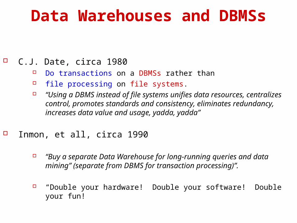
Let’s talk about techniques we use to address these curses.

Horizontal processing of vertically structured data (instead of the ubiquitous vertical processing of horizontal data (record orientation).

Parallelize the engine. Parallelize software engine on clusters of computers.

Parallelize greyware engine on clusters of people (i.e., browser enable all software for visualization)

Why do we need better techniques for data analysis, querying and mining?

Data volume expands by Parkinson’s Law: Data volume expands to fill available data storage

Disk-storage expands by Moore’s law: Available storage doubles every 9 months!

We’re awash with data! Network data: hi-speed, DWDM, All-opt (mgmt, flow classif’n,QoS,security)

10 terabytes by 2004 ~ 1013 B

US EROS Data Center (EDC) archives Earth Observing System (EOS) Remotely Sensed Imagery (RSI), satellite and aerial photo data

15 petabytes by 2007 ~ 1016 B

National Virtual Observatory (aggregated astronomical data) 10 exabytes by 2010 ~ 1019 B

Sensor data from sensors (including Micro & Nano -sensor networks) 10 zettabytes by 2015 ~ 1022 B

WWW (and other text collections) 10 yottabytes by 2020 ~ 1025 B

Genomic/Proteomic/Metabolomic data (microarrays, genechips, genome sequences) 10 gazillabytes by 2030 ~ 1028 B?).

Stock Market prediction data (prices + all the above? especially astronomy data?

10 supragazillabytes by 2040 ~ 1031 B?

Useful information must be teased out of these large volumes of data.

I had to make up these Name! Projected data sizes are overrunning our ability to name those sizes!

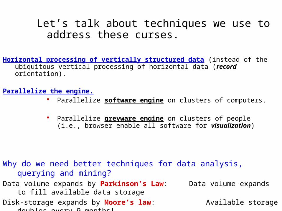
Producer want the color intensity pattern to yield association.One is ”hi_green & low_red hi_yield”. It is very intuitive.

A stronger association was found strictly by analyzing (mining)the data: “hi_NIR & low_redhi_yield”

Once found in historical data (through data mining), producers just query TIFF images mid-season for low_NIR & high_red grid cells, where they then apply additional nitrogen.

This concept can detect ag insurance fraud ( http://www.npr.org/templates/story/story.php?storyId=5013871), forest fires, wetlands drainage, etc.

A Precision Agriculture example

TIFF image Yield Map

and a synchronized yield map (crop yield taken at harvest); thus, 4 feature attributes (B,G,R,Y) and ~100,000 pixels

Yield prediction: dataset consists of an aerial photograph (RGB TIFF image taken during the growing season)

Grasshopper Infestation Prediction (again involving RSI data)

Grasshopper caused significant economic loss each year.

Early infestation prediction is key to damage control.

Pixel classification on remotely sensed imagery holds significant promise to achieve early detection. Pixel classification (signaturing) has many apps: pest detection, fire detection, wet-lands monitoring … (for signaturing we developed the SMILEY software/greyware system) http://midas.cs.ndsu.nodak.edu/~smiley

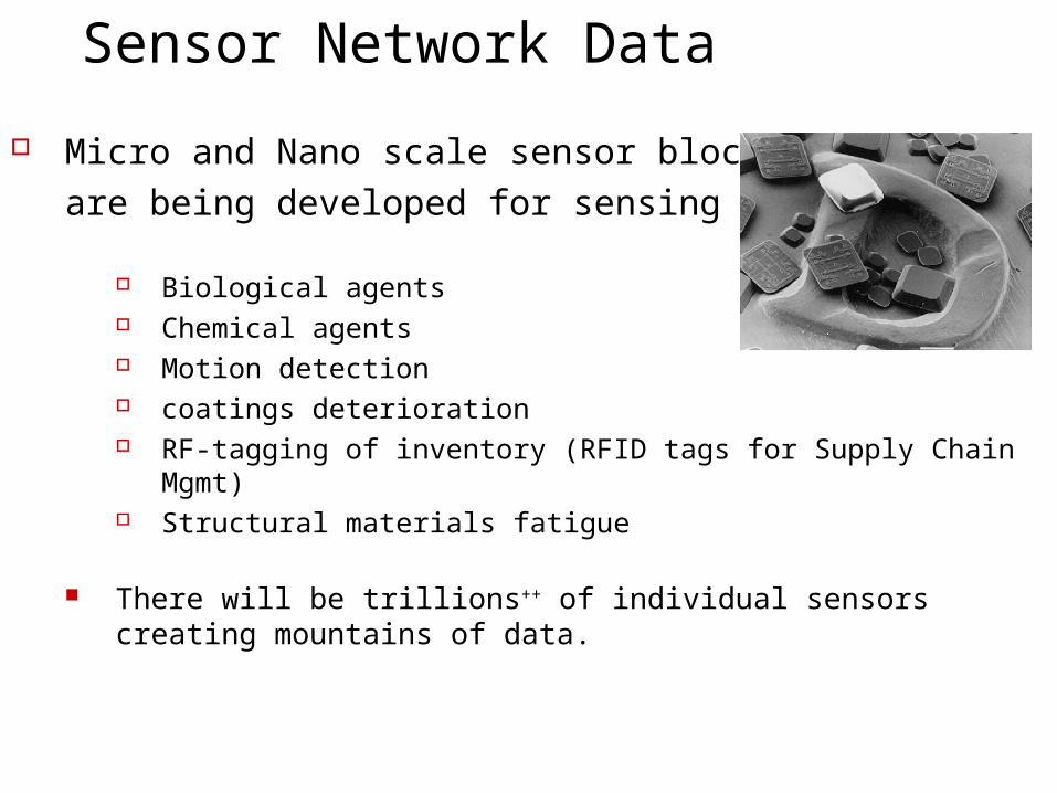
Sensor Network Data

Micro and Nano scale sensor blocksare being developed for sensing

Biological agents Chemical agents Motion detection coatings deterioration RF-tagging of inventory (RFID tags for Supply Chain Mgmt) Structural materials fatigue

There will be trillions++ of individual sensors creating mountains of data.

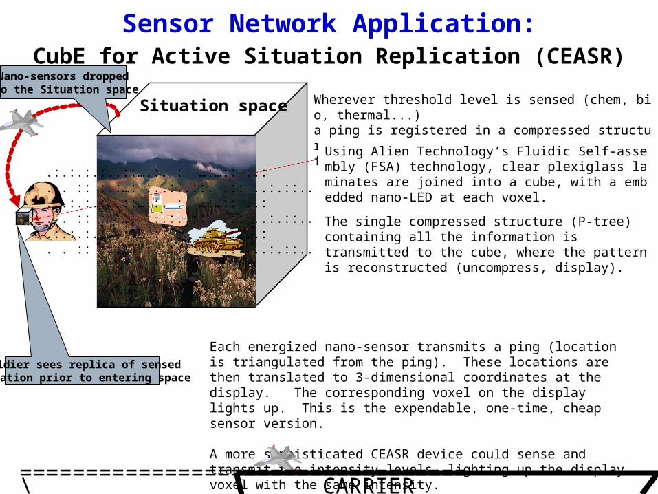
Sensor Network Application:

Each energized nano-sensor transmits a ping (location is triangulated from the ping). These locations are then translated to 3-dimensional coordinates at the display. The corresponding voxel on the display lights up. This is the expendable, one-time, cheap sensor version.

A more sophisticated CEASR device could sense and transmit the intensity levels, lighting up the display voxel with the same intensity.

Wherever threshold level is sensed (chem, bio, thermal...)a ping is registered in a compressed structure (P-tree – detailed definition coming up) for that location.

Situation space

Nano-sensors droppedinto the Situation space

Soldier sees replica of sensedsituation prior to entering space

.:.:.:.:..::….:. : …:…:: ..:

. . :: :.:…: :..:..::. .:: ..:.::..

.:.:.:.:..::….:. : …:…:: ..:

. . :: :.:…: :..:..::. .:: ..:.::..

.:.:.:.:..::….:. : …:…:: ..:

. . :: :.:…: :..:..::. .:: ..:.::..

Using Alien Technology’s Fluidic Self-assembly (FSA) technology, clear plexiglass laminates are joined into a cube, with a embedded nano-LED at each voxel.

==================================\ CARRIER /

CubE for Active Situation Replication (CEASR)

The single compressed structure (P-tree) containing all the information is transmitted to the cube, where the pattern is reconstructed (uncompress, display).

Anthropology Application

Digital Archive Network for Anthropology (DANA)(analyze, query and mine arthropological artifacts (shape, color, discovery location,…)

What is Data Mining

Querying is asking specific questions and expecting specific answers

Data Mining goes into MOUNTAINS of raw data for info gems.

Data Cleaning/Integration:missing data, outliers,noise, errors

Data Warehouse: cleaned, integrated, read-only, periodic, historical raw database

Data Mining

Pattern Evaluation and Assay

OLAPClassificationClusteringRule Mining

Task-relevant Data

SelectionFeature extraction, tuple selection

visualization

Loopbacks

Smart files

Data Mining versus Querying

On the Query end, much work is yet to be done (D. DeWitt, ACM SIGMOD Record’02).

On the Data Mining end, the surface has barely been scratched.But even those scratches had a great impact – One of the early scatchers became the

biggest corporation in the world last year. A Non-scratcher filed for bankruptcy

SQLSELECTFROMWHERE

Complex queries(nested, EXISTS..)

Standard querying

FUZZY query,Search engines,BLAST searches

OLAP (rollup, drilldown, slice/dice..

Searching and Aggregating Machine Learning Data Mining

Supervised Learning – classification regression

Unsupervised Learning - clustering

Walmart vs. KMart

There is a whole spectrum of techniques to get information from data:

Association Rule Mining

Data Prospecting

Fractals, …

Our Approach:Our Approach: Vertical,Vertical, compressed data structures, Predicate-trees or Peano-trees (Ptrees in either case)1 processed horizontally horizontally (DBMSs process horizontal data verticallyhorizontal data vertically)) Ptrees are data-mining-ready, compressed data structures, which attempt to address the

curses of scalability and curse of dimensionality.

1 Ptree Technology is patent pendingby North Dakota State University

6. Lf half of lf of rt? true1

00 0 0 1 1

4. Left half of rt half ? false0 00 0 0

2. Left half pure1? false 0

00 0

1. Whole is pure1? false 0

5. Rt half of right half? true1

00 0 0 1

R11 0 0 0 0 1 0 1 1

Horizontally AND basic Ptrees

Predicate tree technology: vertically project each attribute, Current practice: Structure data into horizontal records. Process vertically (scans)

Top-down construction of the 1-dimensional Ptree representation of R11, denoted, P11, is built by recording the truth of the universal predicate “pure 1” in a tree recursively on halves (1/21 subsets), until purity is achieved.

3. Right half pure1? false 0 00 0

7. Rt half of lf of rt? false0

00 0 0 1 10

0 1 0 1 1 1 1 1 0 0 0 10 1 1 1 1 1 1 1 0 0 0 00 1 0 1 1 0 1 0 1 0 0 10 1 0 1 1 1 1 0 1 1 1 11 0 1 0 1 0 0 0 1 1 0 00 1 0 0 1 0 0 0 1 1 0 11 1 1 0 0 0 0 0 1 1 0 01 1 1 0 0 0 0 0 1 1 0 0

R11 R12 R13 R21 R22 R23 R31 R32 R33 R41 R42 R43

R[A1] R[A2] R[A3] R[A4] 010 111 110 001011 111 110 000010 110 101 001010 111 101 111101 010 001 100010 010 001 101111 000 001 100111 000 001 100

But it is pure (pure0) so this branch ends

then vertically project each bit position of each attribute,then compress each bit slice into a basic Ptree. e.g., compression of R11 into P11 goes as follows:

P11 P12 P13 P21 P22 P23 P31 P32 P33 P41 P42 P43 0 0 0 0 1 10

0 1 0 0 1 01

0 0 00 0 0 1 01 10

0 1 0

0 1 0 1 0

0 0 01 0 01

0 1 0

0 0 0 1 0

0 0 10 1

0 0 10 1 01

0 0 00 1 01

0 0 0 0 1 0 010 01^ ^ ^ ^ ^ ^ ^ ^ ^

0 0 0 0 1 10̂

P11

P11

pure1? false=0

pure1? false=0

pure1? false=0pure1? true=1

And it’s pure so branch ends

pure1? false=0

R(A1 A2 A3 A4)2 7 6 16 7 6 02 7 5 12 7 5 75 2 1 42 2 1 57 0 1 47 0 1 4

Horizontally structuredrecords

Scanned vertically

010 111 110 001011 111 110 000010 110 101 001010 111 101 111101 010 001 100010 010 001 101111 000 001 100111 000 001 100

=

Base 10 Base 2

0 1 0 1 1 1 1 1 0 0 0 10 1 1 1 1 1 1 1 0 0 0 00 1 0 1 1 0 1 0 1 0 0 10 1 0 1 1 1 1 0 1 1 1 11 0 1 0 1 0 0 0 1 1 0 00 1 0 0 1 0 0 0 1 1 0 11 1 1 0 0 0 0 0 1 1 0 01 1 1 0 0 0 0 0 1 1 0 0

R11 R12 R13 R21 R22 R23 R31 R32 R33 R41 R42 R43

R[A1] R[A2] R[A3] R[A4] 010 111 110 001011 111 110 000010 110 101 001010 111 101 111101 010 001 100010 010 001 101111 000 001 100111 000 001 100

To count occurrences of 7,0,1,4 use pure111000001100: 0 P11^P12^P13^P’21^P’22^P’23^P’31^P’32^P33^P41^P’42^P’43 = 0 0

01 ^

7 0 1 4

P11 P12 P13 P21 P22 P23 P31 P32 P33 P41 P42 P43 0 0 0 0 1 10

0 1 0 0 1 01

0 0 00 0 0 1 01 10

0 1 0

0 1 0 1 0

0 0 01 0 01

0 1 0

0 0 0 1 0

0 0 10 1

0 0 10 1 01

0 0 00 1 01

0 0 0 0 1 0 010 01^ ^ ^ ^ ^ ^ ^ ^ ^

R(A1 A2 A3 A4)2 7 6 16 7 6 02 7 5 12 7 5 75 2 1 42 2 1 57 0 1 47 0 1 4

010 111 110 001011 111 110 000010 110 101 001010 111 101 111101 010 001 100010 010 001 101111 000 001 100111 000 001 100

=

This 0 makes entire left branch 0These 0s make this node 0 These 1s and these 0s make this 1

21-level has the only 1-bit so the 1-count = 1*21 = 2

R11 0 0 0 0 1 0 1 1

Top-down construction of basic P-trees is best for understanding, but bottom-up is much more efficient.

Bottom-up construction of 1-Dim, P11, is done using in-order tree traversal and the collapsing of pure siblings, as follow:

0 1 0 1 1 1 1 1 0 0 0 10 1 1 1 1 1 1 1 0 0 0 00 1 0 1 1 0 1 0 1 0 0 10 1 0 1 1 1 1 0 1 1 1 11 0 1 0 1 0 0 0 1 1 0 00 1 0 0 1 0 0 0 1 1 0 11 1 1 0 0 0 0 0 1 1 0 01 1 1 0 0 0 0 0 1 1 0 0

R11 R12 R13 R21 R22 R23 R31 R32 R33 R41 R42 R43

P11

0 0

0

0 0

0

1 0

0

0

0

1 1

1

0

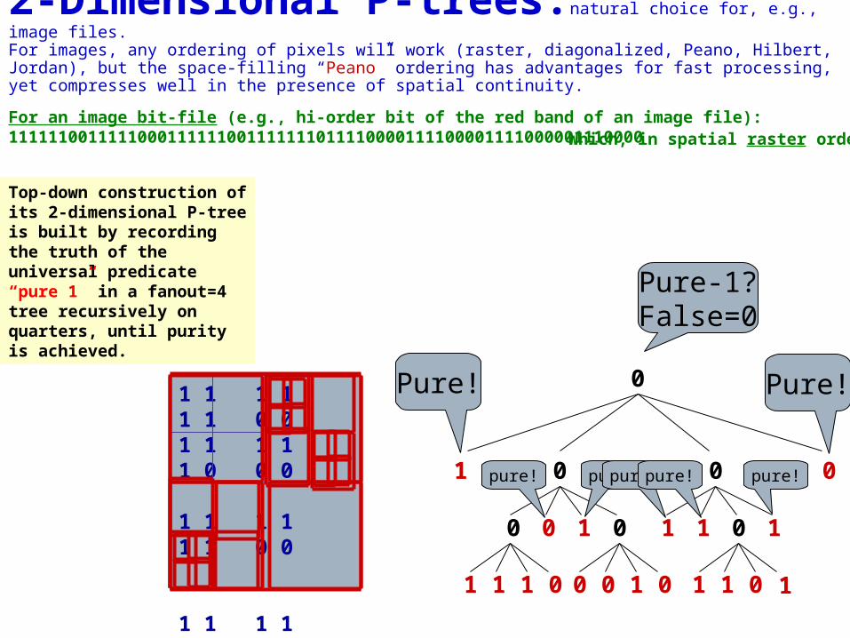
2-Dimensional P-trees:natural choice for, e.g., image files.For images, any ordering of pixels will work (raster, diagonalized, Peano, Hilbert, Jordan), but the space-filling “Peano” ordering has advantages for fast processing, yet compresses well in the presence of spatial continuity.

0

1 0 0 0

0 0 1 0 1 1 0 1

1 1 1 0 0 0 1 0 1 1 0 1

1 1 1 1 1 1 0 01 1 1 1 1 0 0 0 1 1 1 1 1 1 0 0 1 1 1 1 1 1 1 0 1 1 1 1 0 0 0 0 1 1 1 1 0 0 0 0 1 1 1 1 0 0 0 0 0 1 1 1 0 0 0 0

For an image bit-file (e.g., hi-order bit of the red band of an image file):1111110011111000111111001111111011110000111100001111000001110000 Which, in spatial raster order is:

Top-down construction of its 2-dimensional P-tree is built by recording the truth of the universal predicate “pure 1” in a fanout=4 tree recursively on quarters, until purity is achieved.

Pure-1?False=0

Pure!Pure!

pure!pure! pure!pure! pure!

1 1 1 1 1 1 0 01 1 1 1 1 0 0 0 1 1 1 1 1 1 0 0 1 1 1 1 1 1 1 0 1 1 1 1 0 0 0 0 1 1 1 1 0 0 0 0 1 1 1 1 0 0 0 0 0 1 1 1 0 0 0 0

1 1 11

1

1 1 11

1

1 1 11

1

1 1 11

1

1

1 1 10

0

0 0 0 0

0

From here on we will take 4 bit positions at a time, for efficiency.

1 1 1 1

1

0 0 0 1

0

0

1 1 1 1

1

1 1 1 1

1

1 1 0 1

0

1 1 1 1

1

0

0 0 0 0 0 0 0 0 0 0 0 0 0 0 0 0

0 0 0 0

0

Bottom-up construction of the 2-Dimensional P-tree is done using in-order traversal of a fanout=4, log4(64)=4-level tree and the collapsing pure siblings, as follow:

Start here

Node ID (NID) = 2.2.3 Tree levels (going down): 3, 2, 1, 0, with

purity-factors of 43 42 41 40 respectively

Fan-out = 2dimension = 22 = 4

1 1 1 1 1 1 0 01 1 1 1 1 0 0 0 1 1 1 1 1 1 0 0 1 1 1 1 1 1 1 0 1 1 1 1 1 1 1 1 1 1 1 1 1 1 1 1 1 1 1 1 1 1 1 1 0 1 1 1 1 1 1 1

7=111

( 7, 1 ) ( 111, 001 ) 10.10.11

1=001

Some aspects of 2-D P-trees:

0

1 0 0 1

0 0 1 0 0 0 0 1

1 1 1 0 0 0 1 0 1 1 0 1

0 level-3 (pure=43)

1 0 0 1 level-2 (pure=42)

0 0 1 0 1 1 0 1 level-1 (pure=41)

1 1 1 0 0 0 1 0 1 1 0 1 level-0 (pure=40)

0 1 2 3

2

3

2 . 2 . 3

ROOT-COUNT = level-sum * level-purity-factor. Root Count = 7 * 40 + 4 * 41 + 2 * 42 = 55

3-Dimensional Ptrees

12 (1100)022

0 (0000)131

2 (0010)130

15 (1111)121

15 (1111)120

0 (0000)031

2 (0010)030

15 (1111)021

15 (1111)020

12 (1100)113

12 (1100)112

2 (0010)103

12 (1100)102

12 (1100)013

1 (0001)012

4 (0100)003

15 (1111)002

15 (1111)111

15 (1111)110

15 (1111)101

15 (1111)100

15 (1111)011

15 (1111)010

15 (1111)001

15 (1111)000

IntensityZYX

3-Dimensional Ptrees

1

Situation space

How would a CEASR bio-agent detector work?

All other positions contain a 0-bit,i.e., the level of bio-agent detected by the nano-sensors in each of the other 63 cells (voxels) is below the danger threshold.

P

0 0

Start0

00 0001

0

We can save time by noting that all the remaining 56 cells (in 7 other octants) contain all 0s. Each of the next 7 octants will produce eight 0s at the leaf level (8 pure-0 siblings), each of which will collapse to a 0 at level-1. So, proceeding an octant at a time (rather than a cell at a time):

0 0 00 0000

And that position corresponds to the 1-bit position in this cutaway view

at a position, as shown in the situation space.

Suppose a biological agent is sensed by nano-sensors

0

ONE tiny, compressed P-tree can completely represent this “bio-situation” It is constructed (bottom up) as a fan-out=8, level=3 P-tree, as follows.

0 0 00 0000

0

0 0 00 0000

0

0 0 00 0000

0

0 0 00 0000

0

0 0 00 0000

0

0 0 00 0000

0

This entire situation can be transmitted to a personal display unit, as merely two bytes of data plus their two NIDs. For NID, use [level, global_level_offset] rather than [local_segment_offset,…local_segment_offset]. So assume every node not sent is all 0s, that in any 13-bit node segment sent (only need send “mixed” segments), the 1st segment is the level (in this case, need 2 bit only), the next 3 bits give the global_level_offset within that level (i.e., 0..7) and the final 8 bits are the node’s data, then the complete situation can be transmitted as these 13 bits: 01 000 0000 0001

If 2n3 cells (n=2 above) “situation” will take only log2(n) blue, 23n-3 green, 8 red bits

(e.g., even if there are 283=224 ~16,000,000 voxels, transmit merely 3+21+8=32 bits.)

We have now captured the data in the 1st octant (forward-upper-left). Moving to the next octant (forward-upper-right):

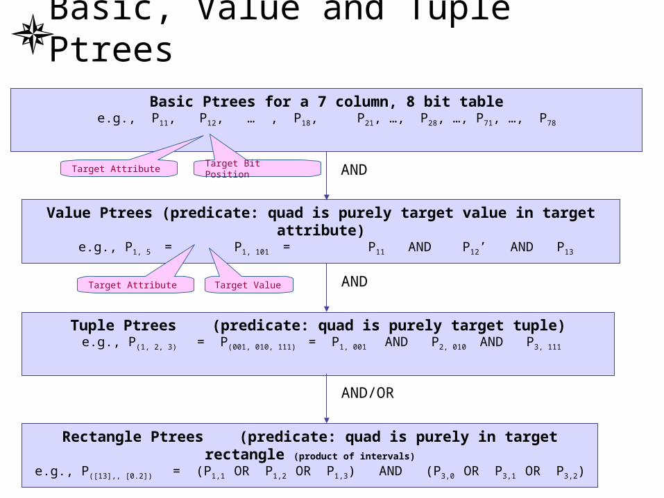
Basic, Value and Tuple Ptrees

Tuple Ptrees (predicate: quad is purely target tuple) e.g., P(1, 2, 3) = P(001, 010, 111) = P1, 001 AND P2, 010 AND P3, 111

AND

Value Ptrees (predicate: quad is purely target value in target attribute) e.g., P1, 5 = P1, 101 = P11 AND P12’ AND P13

AND

Target Attribute Target Value

Basic Ptrees for a 7 column, 8 bit tablee.g., P11, P12, … , P18, P21, …, P28, …, P71, …, P78

Target Attribute Target Bit Position

Rectangle Ptrees (predicate: quad is purely in target rectangle (product of intervals)

e.g., P([13],, [0.2]) = (P1,1 OR P1,2 OR P1,3) AND (P3,0 OR P3,1 OR P3,2)

AND/OR

Horizontal Processing of Vertical Structuresfor Record-based Workloads

For record-based workloads (where the result is a set of records), changing the horizontal record structure and then having to reconstruct it, may introduce too much post processing?

0 1 0 1 1 1 1 1 0 0 0 10 1 1 1 1 1 1 1 0 0 0 00 1 0 1 1 0 1 0 1 0 0 10 1 0 1 1 1 1 0 1 1 1 11 0 1 0 1 0 0 0 1 1 0 00 1 0 0 1 0 0 0 1 1 0 11 1 1 0 0 0 0 0 1 1 0 01 1 1 0 0 0 0 0 1 1 0 0

R11 R12 R13 R21 R22 R23 R31 R32 R33 R41 R42 R43

010 111 110 001011 111 110 000010 110 101 001010 111 101 111101 010 001 100010 010 001 101111 000 001 100111 000 001 100

R( A1 A2 A3 A4)

0 1 0 1 1 1 1 1 0 0 0 10 1 1 1 1 1 1 1 0 0 0 00 1 0 1 1 0 1 0 1 0 0 10 1 0 1 1 1 1 0 1 1 1 11 0 1 0 1 0 0 0 1 1 0 00 1 0 0 1 0 0 0 1 1 0 11 1 1 0 0 0 0 0 1 1 0 01 1 1 0 0 0 0 0 1 1 0 0

R11 R12 R13 R21 R22 R23 R31 R32 R33 R41 R42 R43

1

For data mining workloads, the result is often a bit (Yes/No, True/False) or another unstructured result, where there is no reconstructive post processing?

But even for some standard SQL queries, vertical data may be faster (evaluating when this is true would be an excellent research project)

For example, the SQL query,

SELECT Count * FROM purchases WHERE price $4,000.00 AND 1000 sales 500.

The answer is the root-count of the P-tree resulting from ANDing the price-interval-P-tree, Pprice[4000,) and the sales-interval-P-tree, Psales[500,1000] .

Architecture for the DataMIME™ System

(DataMIMEtm = data mining, NO NOISE) (PDMS = P-tree Data Mining System)

Internet

DII (Data Integration Interface)

Data Integration Language

DIL

YOUR DATA

Data Repositorylossless, compressed, distributed, vertically-

structured database

DMI (Data Mining Interface)

YOUR DATA MINING

Ptree (Predicates) Query Language

PQL

Raster Sorting: Attributes 1st Bit position 2nd

Generalized Raster and Peano Sorting: generalizes to any table with numeric attributes (not just images).

Peano Sorting: Bit position 1st Attributes 2nd

Decimal BinaryUnsorted relation

Generalize Peano Sorting

0

20

40

60

80

100

120

adult

spam

mus

hroo

m

func

tion

crop

Tim

e in

Sec

on

ds

Unsorted

Generalized Raster

Generalized Peano

KNN speed improvement(using 5 UCI Machine Learning Repository data sets)

Astronomy Application: (National Virtual Observatory data)

What Ptree dimension and what ordering should be used for astronomical data?, where all bodies are assumed on surface of celestial sphere (shares equatorial plane with earth and has no specified radius)

Hierarchical Triangle Mesh Tree (HTM-tree, seems to be the accepted standard)

Peano Triangle Mesh Tree (PTM-tree)

Peano Celestial Coordinate tree (RA=Recession Angle (longitudinal angle); dec=declination (latitude angle)

PTM is similar to HTM used in the Sloan Digital Sky Survey project. In both: Sphere is divided into triangles Triangle sides are always great circle segments. PTM differs from HTM in the way in which they are ordered?

The difference between HTM and PTM-trees is in the ordering.

1,2

1,3

1,0

1,1

1

1,3,3

1,3,2

1,3,0

1,3,1

1,2

1,1

1,0

1,3

1

1,1,2

1,1,01,1,1

1.1.3

Ordering of HTM Ordering of PTM-tree

Why use a different ordering?

PTM Triangulation of the Celestial Sphere

Traverse southern hemisphere in the revere direction (just the identical pattern pushed down instead of pulled up, arriving at the Southern neighbor of the start point.

RA

dec

The following ordering produces a sphere-surface filling curve with good continuity characteristics,For each level.

left turn

right

left

right

Equilateral triangle (90o sector) bounded by longitudinal and equatorial line segments

Traverse the next level of triangulation, alternating again with left-turn, right-turn, left-turn, right-turn..

Traverse southern hemisphere in the revere direction (just the identical pattern pushed down instead of pulled up, arriving at the Southern neighbor of the start point.

PTM-triangulation - Next Level

LRLR RLRL LRLR RLRL LRLR RLRL LRLR RLRL LRLR RLRL LRLR RLRL LRLR RLRL LRLR RLRL

South Plane

90o

0o

-90o0o 360o

Plane

Z ZZ Z

Z ZZ Z

Z ZZ Z

Z ZZ Z

Z ZZ Z

Z ZZ Z

Z ZZ Z

Z ZZ Z

Z ZZ Z

Z ZZ Z

Z ZZ Z

Z ZZ Z

Z ZZ Z

Z ZZ Z

Z ZZ Z

Z ZZ Z

Z ZZ Z

Z ZZ Z

Z ZZ Z

Z ZZ Z

Z ZZ Z

Z ZZ Z

Z ZZ Z

Z ZZ Z

Z ZZ Z

Z ZZ Z

Z ZZ Z

Z ZZ Z

Z ZZ Z

Z ZZ Z

Z ZZ Z

Z ZZ Z

Z ZZ Z

Z ZZ Z

Z ZZ Z

Z ZZ Z

Z ZZ Z

Z ZZ Z

Z ZZ Z

Z ZZ Z

Z ZZ Z

Z ZZ Z

Z ZZ Z

Z ZZ Z

Z ZZ Z

Z ZZ Z

Z ZZ Z

Z ZZ Z

Z ZZ Z

Z ZZ Z

Z ZZ Z

Z ZZ Z

Z ZZ Z

Z ZZ Z

Z ZZ Z

Z ZZ Z

Z ZZ Z

Z ZZ Z

Z ZZ Z

Z ZZ Z

Z ZZ Z

Z ZZ Z

Z ZZ Z

Z ZZ Z

Z ZZ Z

Z ZZ Z

Z ZZ Z

Z ZZ Z

Z ZZ Z

Z ZZ Z

Z ZZ Z

Z ZZ Z

Z ZZ Z

Z ZZ Z

Z ZZ Z

Z ZZ Z

Z ZZ Z

Z ZZ Z

Z ZZ Z

Z ZZ Z

Z ZZ Z

Z ZZ Z

Z ZZ Z

Z ZZ Z

Z ZZ Z

Z ZZ Z

Z ZZ Z

Z ZZ Z

Z ZZ Z

Z ZZ Z

Z ZZ Z

Z ZZ Z

Z ZZ Z

Z ZZ Z

Z ZZ Z

Z ZZ Z

Z ZZ Z

Z ZZ Z

Z ZZ Z

Z ZZ Z

Z ZZ Z

Z ZZ Z

Z ZZ Z

Z ZZ Z

Z ZZ Z

Z ZZ Z

Z ZZ Z

Z ZZ Z

Z ZZ Z

Z ZZ Z

Z ZZ Z

Z ZZ Z

Z ZZ Z

Z ZZ Z

Z ZZ Z

Z ZZ Z

Z ZZ Z

Z ZZ Z

Z ZZ Z

Z ZZ Z

Z ZZ Z

Z ZZ Z

Z ZZ Z

Z ZZ Z

Z ZZ Z

Z ZZ Z

Z ZZ Z

Z ZZ Z

Sphere Cylinder

Peano Celestial CoordinatesUnlike PTM-trees which initially partition the sphere into the 8 faces of an octahedron, in the PCCtree scheme:Sphere is tranformed to a cylinder, then into a rectangle, then standard Peano ordering is used on the Celestial Coordinates. Celestial Coordinates Recession Angle (RA) runs from 0 to 360o dand Declination Angle (dec) runs from -90o to 90o.

e0

e1

e2

e3

1 0 1 1

0 1 1 1

1 1 0 1

1 0 1 0

0

1 01

1 0 01

0 1 01

1 0 00

1 1 1 1

1 0 0 1

0 1 0 01 0 1 1

o1

o2

o3

o0

Gene-Experiment-Organism Cube (1 iff that gene from that organism expresses at a threshold level in that experiment.) many-to-many-to-many relationship

Organism Dimension Table

30001Musmusculus

mouse

12.10Saccharomyces

cerevisiae

yeast

1850Drosophilamelanogaster

fly

30001Homo sapienshuman

Genome Size (million bp)

VertSpeciesOrganism Gene Dimension Table

0011PolyA-Tail

.9.1.1.1StopCodonDensity

apopmitomeioapopFunction

RiboNuclRiboMytaSubCell-Location

Experiment Dimension Table (MIAME)

1asa42

1aca42

0hsb22

1hca23

NMHSAD

ED

STZ

CTY

STR

UNV

PI

LAB

g0 g1 g2 g3

e0

e1

e2

e3

17, 78 12, 60 Mi, 40 1, 48

10, 75 0 0 7, 40

0 14, 65 0 0

16, 76 0 9, 45 Pl, 43

Gene-Organism Dimension Table (chromosome,length)

PUBLIC (Ptree Unfied BioLogicalInformtiCs Data Cube andDimension Tables)

0 1 0 0

0 1 0 1

0 1 1 0

1 0 0 1

1 0 0

0 1 1

0 1 1

0 1

0 10

g0

g1

g2

g3

g0

g1

g2

g3

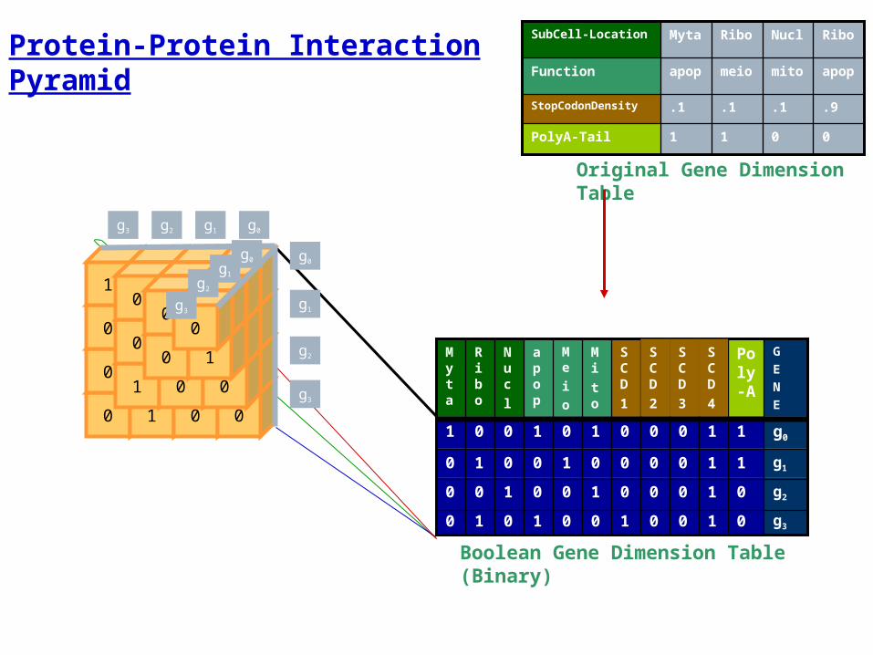
Protein-Protein Interaction Pyramid

Original Gene Dimension Table

0011PolyA-Tail

.9.1.1.1StopCodonDensity

apopmitomeioapopFunction

RiboNuclRiboMytaSubCell-Location

g0g1g2g3

g301001001010

g201000100100

g111000010010

g011000101001

GENE

Poly-A

SCD1

Mito

Meio

apop

Nucl

Ribo

Myta

SCD2

SCD3

SCD4

Boolean Gene Dimension Table (Binary)

Association of Computing Machinery KDD-Cup-02Association of Computing Machinery KDD-Cup-02

NDSU Team

Network Security Application(Network security through Vertical Structured data)

Network layers do their own partitioning Packets, frames, etc. (usually independent of any intrinsic data structuring – e.g., record structure)

Fragmentation/Reassembly, Segmentation/Reassembly

Data privacy is compromised when the horizontal (stream) message content is eavesdropped upon at the reassembled level (in network

A standard solution is to host-encrypt the horizontal structure so that any network reassembled message is meaningless.

Alt.: Vertically structure (decompose, partition) data (e.g., basic Ptrees). Send one Ptree per packet Send intra-message packets separately

Trick flow classifiers into thinking the multiple packets associated with a particular message are unrelated.

The message is only meaningful after destination demux-ing Note: the only basic Ptree that holds actual information is the high-order bit Ptree. Therefore

encrypt it! There is a whole passel of killer ideas associated with the concept of using vertical structuring data within

network transmission units Active networking? (AND basic Ptrees (or just certain levels of) at active net nodes?)

Network Security Application Cont.

Vertically structure (decompose, partition) data (e.g., basic Ptrees). Send one P-tree (vertical bit-slice per packet Send basic P-tree slices (for a given attribute) one at a

time starting with the low order bit slice. Encrypt it using some agreed upon algorithm (and

key) (requires key distribution) But then steganographically embed the crypto alg

identity and key structure for the next higher order bit into the ptree (as the carrier message).

Continue to do that for each higher order bit until you get to the highest order bit. Until it arrives and unless each crypto has been broken (in time to apply it to the next level) the message is un-decipherable.