Embed Size (px)
Citation preview

Data Visualization (CIS 468)
Data
Dr David Koop
D Koop CIS 468 Fall 2018
xkcd on Curve-Fitting
2
[xkcd]D Koop CIS 468 Fall 2018
Including JavaScript in HTMLbull Use the script tag bull Can either inline JavaScript or load it from an external file
- ltscript type=textjavascriptgt a = 5 b = 8 c = a b + b - a ltscriptgt ltscript type=textjavascript src=scriptjsgt
bull The order the javascript is executed is the order it is executed bull Example in the above scriptjs can access the variables a b and c
3D Koop CIS 468 Fall 2018
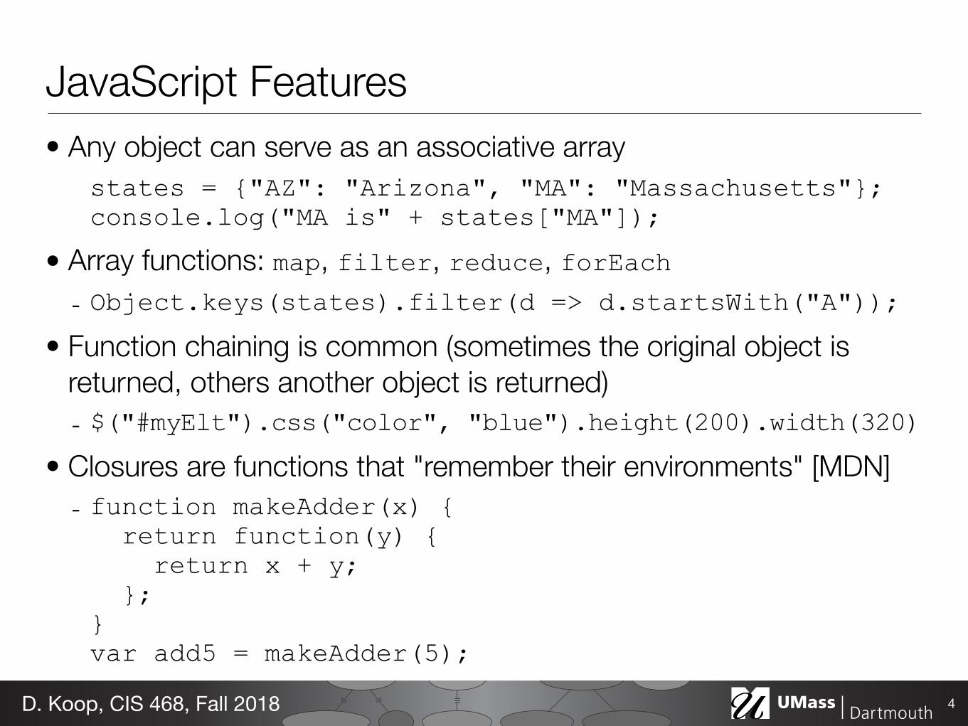
JavaScript Featuresbull Any object can serve as an associative array
states = AZ Arizona MA Massachusettsconsolelog(MA is + states[MA])
bull Array functions map filter reduce forEach - Objectkeys(states)filter(d =gt dstartsWith(A))
bull Function chaining is common (sometimes the original object is returned others another object is returned) - $(myElt)css(color blue)height(200)width(320)
bull Closures are functions that remember their environments [MDN] - function makeAdder(x) return function(y) return x + y var add5 = makeAdder(5)
4D Koop CIS 468 Fall 2018
Using Array Functionsbull var a = [2 4 7 11 22 84]
bull Named function - function isEven(d) return (d 2 == 0) afilter(isEven)
bull Anonymous function - afilter(function(d) return (d 2 == 0) )
bull Arrow function - afilter(d =gt (d 2 == 0))
5D Koop CIS 468 Fall 2018
Manipulating the DOM with JavaScriptbull Key global variables
bull window Global namespace bull document Current document bull documentgetElementById(hellip) Get an element via its id
bull HTML is parsed into an in-memory document (DOM) bull Can access and modify information stored in the DOM bull Can add information to the DOM
6D Koop CIS 468 Fall 2018
Example JavaScript and the DOMbull Start with no real content just divs ltdiv id=firstSectiongtltdivgt ltdiv id=secondSectiongtltdivgt ltdiv id=finalSectiongtltdivgt
bull Get existing elements - documentquerySelector - documentgetElementById
bull Programmatically add elements - documentcreateElement - documentcreateTextNode - ElementappendChild - ElementsetAttribute
bull Link
7D Koop CIS 468 Fall 2018
Creating SVG figures via JavaScriptbull SVG elements can be accessed and modified just like HTML
elements bull Create a new SVG programmatically and add it into a page
- var divElt = documentgetElementById(chart)var svg = documentcreateElementNS( httpwwww3org2000svg svg)divEltappendChild(svg)
bull You can assign attributes - svgsetAttribute(height 400) svgsetAttribute(width 600) svgCirclesetAttribute(r 50)
8D Koop CIS 468 Fall 2018
SVG Manipulation Examplebull Draw a horizontal bar chart
- var a = [6 2 6 10 7 18 0 17 20 6] bull Steps
9D Koop CIS 468 Fall 2018
SVG Manipulation Examplebull Draw a horizontal bar chart
- var a = [6 2 6 10 7 18 0 17 20 6] bull Steps
- Programmatically create SVG - Create individual rectangle for each item
10D Koop CIS 468 Fall 2018
Manipulating SVG via JavaScriptbull SVG can be navigated just like the DOM bull Example
function addEltToSVG(svg name attrs) var element = documentcreateElementNS( httpwwww3org2000svg name) if (attrs === undefined) attrs = for (var key in attrs) elementsetAttribute(key attrs[key]) svgappendChild(element) mysvg = documentgetElementById(mysvg) addEltToSVG(mysvg rect x 50 y 50 width 40height 40 fill blue)
11D Koop CIS 468 Fall 2018
SVG Manipulation Examplebull Possible Solution
- httpcodepeniodakooppenGrdBjE
12D Koop CIS 468 Fall 2018
Assignment 1bull httpwwwcisumassdedu
~dkoopcis468-2018faassignment1html
bull Due next Tuesday (Sept 25) bull HTML CSS SVG JavaScript bull Questions
13D Koop CIS 468 Fall 2018
ldquoComputer-based visualization systems provide visual representations of datasets designed to help people carry out tasks more effectivelyrdquo
mdash T Munzner
14D Koop CIS 468 Fall 2018
Databull What is this data
bull Semantics real-world meaning of the data bull Type structural or mathematical interpretation bull Both often require metadata
- Sometimes we can infer some of this information - Line between data and metadata isnrsquot always clear
15D Koop CIS 468 Fall 2018
Data
16D Koop CIS 468 Fall 2018
Data Terminologybull Items
- An item is an individual discrete entity - eg row in a table node in a network
bull Attributes - An attribute is some specific property that can be measured
observed or logged - aka variable (data) dimension - eg a column in a table
17D Koop CIS 468 Fall 2018
Semanticsbull The meaning of the databull Example 94023 90210 52790 02747
18D Koop CIS 468 Fall 2018
Semanticsbull The meaning of the databull Example 94023 90210 52790 02747
- Attendance at college football games
18D Koop CIS 468 Fall 2018
Semanticsbull The meaning of the databull Example 94023 90210 52790 02747
- Attendance at college football games- Salaries
18D Koop CIS 468 Fall 2018
Semanticsbull The meaning of the databull Example 94023 90210 52790 02747
- Attendance at college football games- Salaries- Zip codes
bull Cannot always infer based on what the data looks likebull Often require semantics to better understand databull Column names help with semanticsbull May also include rules about data a zip code is part of an address
that uniquely identifies a residencebull Useful for asking good questions about the data
18D Koop CIS 468 Fall 2018
Items amp Attributes
19
22
Fieldattribute
item
D Koop CIS 468 Fall 2018
Data Typesbull Nodes
- Synonym for item but in the context of networks (graphs) bull Links
- A link is a relation between two items - eg social network friends computer network links
20D Koop CIS 468 Fall 2018
Items amp Links
21
[Bostock 2011]D Koop CIS 468 Fall 2018
Item
Links
Data Typesbull Positions
- A position is a location in space (usually 2D or 3D) - May be subject to projections - eg cities on a map a sampled region in an CT scan
bull Grids - A grid specifies how data is sampled both geometrically and
topologically - eg how CT scan data is stored
22D Koop CIS 468 Fall 2018
Positions and Grids
23D Koop CIS 468 Fall 2018
Position Grid
Dataset Types
24
Tables
Attributes (columns)
Items (rows)
Cell containing value
Networks
Link
Node (item)
Trees
Fields (Continuous)
Attributes (columns)
Value in cell
Cell
Multidimensional Table
Value in cell
Grid of positions
Geometry (Spatial)
Position
Dataset Types
[Munzner (ill Maguire) 2014]D Koop CIS 468 Fall 2018
Tables
25
Fieldattribute
itemcell
D Koop CIS 468 Fall 2018
Attribute SemanticsKeys vs Values (Tables) or Independent vs Dependent (Fields)
Flat
Multidimensional
Tabl
es
Fiel
ds
Tablesbull Data organized by rows amp columns
- row ~ item (usually) - column ~ attribute - label ~ attribute name
bull Key identifies each item (row) - Usually unique - Allows join of data from 2+ tables - Compound key key split among
multiple columns eg (state year) for population
bull Multidimensional - Split compound key - eg a data cube with (state year)
26
[Munzner (ill Maguire) 2014]D Koop CIS 468 Fall 2018
Table Visualizations
27
0
0
0
0
0
0
00
5
5
5
5
5
5
55
10
10
10
10
10
10
1010
15
15
15
15
15
15
1515
20
20
20
20
20
20
2020
25
25
25
25
25
25
2525
30
30
30
30
30
30
3030
35
35
35
35
35
35
3535
40
40
40
40
40
40
4040
45
45
45
45
45
45
4545
economy (mpg)
economy (mpg)
economy (mpg)
economy (mpg)
economy (mpg)
economy (mpg)
economy (mpg)economy (mpg)
30
30
30
30
30
30
3030
35
35
35
35
35
35
3535
40
40
40
40
40
40
4040
45
45
45
45
45
45
4545
50
50
50
50
50
50
5050
55
55
55
55
55
55
5555
60
60
60
60
60
60
6060
65
65
65
65
65
65
6565
70
70
70
70
70
70
7070
75
75
75
75
75
75
7575
80
80
80
80
80
80
8080cylinders
cylinders
cylinders
cylinders
cylinders
cylinders
cylinderscylinders
100
100
100
100
100
100
100100
150
150
150
150
150
150
150150
200
200
200
200
200
200
200200
250
250
250
250
250
250
250250
300
300
300
300
300
300
300300
350
350
350
350
350
350
350350
400
400
400
400
400
400
400400
450
450
450
450
450
450
450450
displacement (cc)
displacement (cc)
displacement (cc)
displacement (cc)
displacement (cc)
displacement (cc)
displacement (cc)displacement (cc)
0
0
0
0
0
0
00
20
20
20
20
20
20
2020
40
40
40
40
40
40
4040
60
60
60
60
60
60
6060
80
80
80
80
80
80
8080
100
100
100
100
100
100
100100
120
120
120
120
120
120
120120
140
140
140
140
140
140
140140
160
160
160
160
160
160
160160
180
180
180
180
180
180
180180
200
200
200
200
200
200
200200
220
220
220
220
220
220
220220
power (hp)
power (hp)
power (hp)
power (hp)
power (hp)
power (hp)
power (hp)power (hp)
2000
2000
2000
2000
2000
2000
20002000
2500
2500
2500
2500
2500
2500
25002500
3000
3000
3000
3000
3000
3000
30003000
3500
3500
3500
3500
3500
3500
35003500
4000
4000
4000
4000
4000
4000
40004000
4500
4500
4500
4500
4500
4500
45004500
5000
5000
5000
5000
5000
5000
50005000
weight (lb)
weight (lb)
weight (lb)
weight (lb)
weight (lb)
weight (lb)
weight (lb)weight (lb)
8
8
8
8
8
8
88
10
10
10
10
10
10
1010
12
12
12
12
12
12
1212
14
14
14
14
14
14
1414
16
16
16
16
16
16
1616
18
18
18
18
18
18
1818
20
20
20
20
20
20
2020
22
22
22
22
22
22
2222
24
24
24
24
24
24
2424
0-60 mph (s)
0-60 mph (s)
0-60 mph (s)
0-60 mph (s)
0-60 mph (s)
0-60 mph (s)
0-60 mph (s)0-60 mph (s)
70
70
70
70
70
70
7070
71
71
71
71
71
71
7171
72
72
72
72
72
72
7272
73
73
73
73
73
73
7373
74
74
74
74
74
74
7474
75
75
75
75
75
75
7575
76
76
76
76
76
76
7676
77
77
77
77
77
77
7777
78
78
78
78
78
78
7878
79
79
79
79
79
79
7979
80
80
80
80
80
80
8080
81
81
81
81
81
81
8181
82
82
82
82
82
82
8282year
year
year
year
year
year
yearyear
[M Bostock 2011]D Koop CIS 468 Fall 2018
Networksbull Why networks instead of graphs bull Tables can represent networks
- Many-many relationships - Also can be stored as specific
graph databases or files
28D Koop CIS 468 Fall 2018
Networks
29
Danny Holten amp Jarke J van Wijk Force-Directed Edge Bundling for Graph Visualization
Figure 7 US airlines graph (235 nodes 2101 edges) (a) not bundled and bundled using (b) FDEB with inverse-linear model(c) GBEB and (d) FDEB with inverse-quadratic model
Figure 8 US migration graph (1715 nodes 9780 edges) (a) not bundled and bundled using (b) FDEB with inverse-linearmodel (c) GBEB and (d) FDEB with inverse-quadratic model The same migration flow is highlighted in each graph
Figure 9 A low amount of straightening provides an indication of the number of edges comprising a bundle by widening thebundle (a) s = 0 (b) s = 10 and (c) s = 40 If s is 0 color more clearly indicates the number of edges comprising a bundle
we generated use the rendering technique described in Sec-tion 41 To facilitate the comparison of migration flow inFigure 8 we use a similar rendering technique as the onethat Cui et al [CZQ08] used to generate Figure 8c
The airlines graph is comprised of 235 nodes and 2101edges It took 19 seconds to calculate the bundled airlinesgraphs (Figures 7b and 7d) using the calculation scheme pre-
sented in Section 33 The migration graph is comprised of1715 nodes and 9780 edges It took 80 seconds to calculatethe bundled migration graphs (Figures 8b and 8d) using thesame calculation scheme All measurements were performedon an Intel Core 2 Duo 266GHz PC running Windows XPwith 2GB of RAM and a GeForce 8800GT graphics cardOur prototype was implemented in Borland Delphi 7
c 2009 The Author(s)Journal compilation c 2009 The Eurographics Association and Blackwell Publishing Ltd
[Holten amp van Wijk 2009]D Koop CIS 468 Fall 2018
Networks
30
[Holten amp van Wijk 2009]D Koop CIS 468 Fall 2018
Danny Holten amp Jarke J van Wijk Force-Directed Edge Bundling for Graph Visualization
Figure 7 US airlines graph (235 nodes 2101 edges) (a) not bundled and bundled using (b) FDEB with inverse-linear model(c) GBEB and (d) FDEB with inverse-quadratic model
Figure 8 US migration graph (1715 nodes 9780 edges) (a) not bundled and bundled using (b) FDEB with inverse-linearmodel (c) GBEB and (d) FDEB with inverse-quadratic model The same migration flow is highlighted in each graph
Figure 9 A low amount of straightening provides an indication of the number of edges comprising a bundle by widening thebundle (a) s = 0 (b) s = 10 and (c) s = 40 If s is 0 color more clearly indicates the number of edges comprising a bundle
we generated use the rendering technique described in Sec-tion 41 To facilitate the comparison of migration flow inFigure 8 we use a similar rendering technique as the onethat Cui et al [CZQ08] used to generate Figure 8c
The airlines graph is comprised of 235 nodes and 2101edges It took 19 seconds to calculate the bundled airlinesgraphs (Figures 7b and 7d) using the calculation scheme pre-
sented in Section 33 The migration graph is comprised of1715 nodes and 9780 edges It took 80 seconds to calculatethe bundled migration graphs (Figures 8b and 8d) using thesame calculation scheme All measurements were performedon an Intel Core 2 Duo 266GHz PC running Windows XPwith 2GB of RAM and a GeForce 8800GT graphics cardOur prototype was implemented in Borland Delphi 7
c 2009 The Author(s)Journal compilation c 2009 The Eurographics Association and Blackwell Publishing Ltd
Fields
31D Koop CIS 468 Fall 2018
Scalar Fields Vector Fields Tensor Fields
Each point in space has an associated
Vector Fields
s0
2
400 01 02
10 11 12
20 21 22
3
5
2
4v0
v1
v2
3
5
Fields
31D Koop CIS 468 Fall 2018
Scalar Fields Vector Fields Tensor Fields(Order-1 Tensor Fields)(Order-0 Tensor Fields) (Order-2+)
Each point in space has an associated
Scalar
Vector Fields
Vector Tensor
Fieldsbull Difference between continuous and discrete values bull Examples temperature pressure density bull Grids necessary to sample continuous data
bull Interpolation ldquohow to show values between the sampled points in ways that do not misleadrdquo
32D Koop CIS 468 Fall 2018
Grids (Meshes)bull Meshes combine positional information (geometry) with
topological information (connectivity)
bull Mesh type can differ substantial depending in the way mesh cells are formed
From Weiskopf Machiraju Moumlllercopy WeiskopfMachirajuMoumlller
Data Structures
bull Grid typesndash Grids differ substantially in the cells (basic
building blocks) they are constructed from and in the way the topological information is given
scattered uniform rectilinear structured unstructured[Weiskopf Machiraju Moumlller]
Spatial Data Example MRI
33
[via Levine 2014]D Koop CIS 468 Fall 2018
Scivis and Infovisbull Two subfields of visualization bull Scivis deals with data where the spatial position is given with data
- Usually continuous data - Often displaying physical phenonema - Techniques like isosurfacing volume rendering vector field vis
bull In Infovis the data has no set spatial representation designer chooses how to visually represent data
bull Also compare background colors of visualizations )
34D Koop CIS 468 Fall 2018
SciVis
35
[Google Image Search for scientific visualization 2017]D Koop CIS 468 Fall 2018
InfoVis
36
[Google Image Search for information visualization 2017]D Koop CIS 468 Fall 2018
Sets amp Lists
37
[Daniels httpexperimentsundercurrentcom]D Koop CIS 468 Fall 2018
Attribute Types
38
Attributes
Attribute Types
Ordering Direction
Categorical Ordered
Ordinal Quantitative
Sequential Diverging Cyclic
[Munzner (ill Maguire) 2014]D Koop CIS 468 Fall 2018
Categorial Ordinal and Quantitative
39
231 = Quantitative2 = Nominal3 = Ordinal
quantitative ordinal categorical
D Koop CIS 468 Fall 2018
Categorial Ordinal and Quantitative
40
241 = Quantitative2 = Nominal3 = Ordinal
quantitative ordinal categorical
D Koop CIS 468 Fall 2018
Ordering Direction
41
Attributes
Attribute Types
Ordering Direction
Categorical Ordered
Ordinal Quantitative
Sequential Diverging Cyclic
[Munzner (ill Maguire) 2014]D Koop CIS 468 Fall 2018
Sequential and Diverging Databull Sequential homogenous range
from a minimum to a maximum - Examples Land elevations ocean
depths bull Diverging can be deconstructed
into two sequences pointing in opposite directions - Has a zero point (not necessary 0) - Example Map of both land
elevation and ocean depth
42
[Rogowitz amp Treinish 1998]D Koop CIS 468 Fall 2018
Cyclic Data
43
lar structure of spirals allows for an easy detection of cyclesand for the comparison of periodic data sets Furthermorethe continuity of the data is expressed by using a spiral in-stead of a circle
31 Mathematical description and types of spirals
A spiral is easy to describe and understand in polar coor-dinates ie in the form The distinctive feature ofa spiral is that f is a monotone function In this work we as-sume a spiral is described by
Several simple functions f lead to well-known types ofspirals bull Archimedeslsquo spiral has the form It has the spe-
cial property that a ray emanating from the origincrosses two consecutive arcs of the spiral in a constantdistance
bull The Hyperbolic spiral has the form It is theinverse of Archimedeslsquo spiral with respect to the origin
bull More generally spirals of the form are calledArchimedean spirals
bull The logarithmic spiral has the form It has thespecial property that all arcs cut a ray emanating fromthe origin under the same angleFor the visualization of time-dependent data Archimedeslsquo
spiral seems to be the most appropriate In most applicationsdata from different periods are equally important Thisshould be reflected visually in that the distance to other peri-ods is always the same
32 Mapping data to the spiral
In general markers bars and line elements can be usedto visualize time-series data similar to standard point barand line graphs on Spiral Graphs For instance quantitativediscrete data can be presented as bars on the spiral or bymarks with a corresponding distance to the spiral Howeversince the x and y coordinate are needed to achieve the generalform of the spiral their use is limited for the display of datavalues One might consider to map data values to small ab-solute changes in the radius ie
Yet we have found this way of visualizing to be ineffec-tive We conclude that the general shape of the spiral shouldbe untouched and other attributes should be used such asbull colourbull texture including line styles and patterns
Figure 1Two visualizations of sunshine intensity using about the same screen real estate and thesame color coding scheme In the spiral visualization it is much easier to compare days to spotcloudy time periods or to see events like sunrise and sunset
r f ϕ( )=
r f ϕ( ) dfdϕ------ 0 ϕ R+isingt=
r aϕ=
2πar a ϕfrasl=
r aϕk=
r aekϕ=
r aϕ bv ϕ( ) b πamax v ϕ( )( )---------------------------lt+=
[Sunlight intensity Weber et al 2001]D Koop CIS 468 Fall 2018

xkcd on Curve-Fitting
2
[xkcd]D Koop CIS 468 Fall 2018
Including JavaScript in HTMLbull Use the script tag bull Can either inline JavaScript or load it from an external file
- ltscript type=textjavascriptgt a = 5 b = 8 c = a b + b - a ltscriptgt ltscript type=textjavascript src=scriptjsgt
bull The order the javascript is executed is the order it is executed bull Example in the above scriptjs can access the variables a b and c
3D Koop CIS 468 Fall 2018
JavaScript Featuresbull Any object can serve as an associative array
states = AZ Arizona MA Massachusettsconsolelog(MA is + states[MA])
bull Array functions map filter reduce forEach - Objectkeys(states)filter(d =gt dstartsWith(A))
bull Function chaining is common (sometimes the original object is returned others another object is returned) - $(myElt)css(color blue)height(200)width(320)
bull Closures are functions that remember their environments [MDN] - function makeAdder(x) return function(y) return x + y var add5 = makeAdder(5)
4D Koop CIS 468 Fall 2018
Using Array Functionsbull var a = [2 4 7 11 22 84]
bull Named function - function isEven(d) return (d 2 == 0) afilter(isEven)
bull Anonymous function - afilter(function(d) return (d 2 == 0) )
bull Arrow function - afilter(d =gt (d 2 == 0))
5D Koop CIS 468 Fall 2018
Manipulating the DOM with JavaScriptbull Key global variables
bull window Global namespace bull document Current document bull documentgetElementById(hellip) Get an element via its id
bull HTML is parsed into an in-memory document (DOM) bull Can access and modify information stored in the DOM bull Can add information to the DOM
6D Koop CIS 468 Fall 2018
Example JavaScript and the DOMbull Start with no real content just divs ltdiv id=firstSectiongtltdivgt ltdiv id=secondSectiongtltdivgt ltdiv id=finalSectiongtltdivgt
bull Get existing elements - documentquerySelector - documentgetElementById
bull Programmatically add elements - documentcreateElement - documentcreateTextNode - ElementappendChild - ElementsetAttribute
bull Link
7D Koop CIS 468 Fall 2018
Creating SVG figures via JavaScriptbull SVG elements can be accessed and modified just like HTML
elements bull Create a new SVG programmatically and add it into a page
- var divElt = documentgetElementById(chart)var svg = documentcreateElementNS( httpwwww3org2000svg svg)divEltappendChild(svg)
bull You can assign attributes - svgsetAttribute(height 400) svgsetAttribute(width 600) svgCirclesetAttribute(r 50)
8D Koop CIS 468 Fall 2018
SVG Manipulation Examplebull Draw a horizontal bar chart
- var a = [6 2 6 10 7 18 0 17 20 6] bull Steps
9D Koop CIS 468 Fall 2018
SVG Manipulation Examplebull Draw a horizontal bar chart
- var a = [6 2 6 10 7 18 0 17 20 6] bull Steps
- Programmatically create SVG - Create individual rectangle for each item
10D Koop CIS 468 Fall 2018
Manipulating SVG via JavaScriptbull SVG can be navigated just like the DOM bull Example
function addEltToSVG(svg name attrs) var element = documentcreateElementNS( httpwwww3org2000svg name) if (attrs === undefined) attrs = for (var key in attrs) elementsetAttribute(key attrs[key]) svgappendChild(element) mysvg = documentgetElementById(mysvg) addEltToSVG(mysvg rect x 50 y 50 width 40height 40 fill blue)
11D Koop CIS 468 Fall 2018
SVG Manipulation Examplebull Possible Solution
- httpcodepeniodakooppenGrdBjE
12D Koop CIS 468 Fall 2018
Assignment 1bull httpwwwcisumassdedu
~dkoopcis468-2018faassignment1html
bull Due next Tuesday (Sept 25) bull HTML CSS SVG JavaScript bull Questions
13D Koop CIS 468 Fall 2018
ldquoComputer-based visualization systems provide visual representations of datasets designed to help people carry out tasks more effectivelyrdquo
mdash T Munzner
14D Koop CIS 468 Fall 2018
Databull What is this data
bull Semantics real-world meaning of the data bull Type structural or mathematical interpretation bull Both often require metadata
- Sometimes we can infer some of this information - Line between data and metadata isnrsquot always clear
15D Koop CIS 468 Fall 2018
Data
16D Koop CIS 468 Fall 2018
Data Terminologybull Items
- An item is an individual discrete entity - eg row in a table node in a network
bull Attributes - An attribute is some specific property that can be measured
observed or logged - aka variable (data) dimension - eg a column in a table
17D Koop CIS 468 Fall 2018
Semanticsbull The meaning of the databull Example 94023 90210 52790 02747
18D Koop CIS 468 Fall 2018
Semanticsbull The meaning of the databull Example 94023 90210 52790 02747
- Attendance at college football games
18D Koop CIS 468 Fall 2018
Semanticsbull The meaning of the databull Example 94023 90210 52790 02747
- Attendance at college football games- Salaries
18D Koop CIS 468 Fall 2018
Semanticsbull The meaning of the databull Example 94023 90210 52790 02747
- Attendance at college football games- Salaries- Zip codes
bull Cannot always infer based on what the data looks likebull Often require semantics to better understand databull Column names help with semanticsbull May also include rules about data a zip code is part of an address
that uniquely identifies a residencebull Useful for asking good questions about the data
18D Koop CIS 468 Fall 2018
Items amp Attributes
19
22
Fieldattribute
item
D Koop CIS 468 Fall 2018
Data Typesbull Nodes
- Synonym for item but in the context of networks (graphs) bull Links
- A link is a relation between two items - eg social network friends computer network links
20D Koop CIS 468 Fall 2018
Items amp Links
21
[Bostock 2011]D Koop CIS 468 Fall 2018
Item
Links
Data Typesbull Positions
- A position is a location in space (usually 2D or 3D) - May be subject to projections - eg cities on a map a sampled region in an CT scan
bull Grids - A grid specifies how data is sampled both geometrically and
topologically - eg how CT scan data is stored
22D Koop CIS 468 Fall 2018
Positions and Grids
23D Koop CIS 468 Fall 2018
Position Grid
Dataset Types
24
Tables
Attributes (columns)
Items (rows)
Cell containing value
Networks
Link
Node (item)
Trees
Fields (Continuous)
Attributes (columns)
Value in cell
Cell
Multidimensional Table
Value in cell
Grid of positions
Geometry (Spatial)
Position
Dataset Types
[Munzner (ill Maguire) 2014]D Koop CIS 468 Fall 2018
Tables
25
Fieldattribute
itemcell
D Koop CIS 468 Fall 2018
Attribute SemanticsKeys vs Values (Tables) or Independent vs Dependent (Fields)
Flat
Multidimensional
Tabl
es
Fiel
ds
Tablesbull Data organized by rows amp columns
- row ~ item (usually) - column ~ attribute - label ~ attribute name
bull Key identifies each item (row) - Usually unique - Allows join of data from 2+ tables - Compound key key split among
multiple columns eg (state year) for population
bull Multidimensional - Split compound key - eg a data cube with (state year)
26
[Munzner (ill Maguire) 2014]D Koop CIS 468 Fall 2018
Table Visualizations
27
0
0
0
0
0
0
00
5
5
5
5
5
5
55
10
10
10
10
10
10
1010
15
15
15
15
15
15
1515
20
20
20
20
20
20
2020
25
25
25
25
25
25
2525
30
30
30
30
30
30
3030
35
35
35
35
35
35
3535
40
40
40
40
40
40
4040
45
45
45
45
45
45
4545
economy (mpg)
economy (mpg)
economy (mpg)
economy (mpg)
economy (mpg)
economy (mpg)
economy (mpg)economy (mpg)
30
30
30
30
30
30
3030
35
35
35
35
35
35
3535
40
40
40
40
40
40
4040
45
45
45
45
45
45
4545
50
50
50
50
50
50
5050
55
55
55
55
55
55
5555
60
60
60
60
60
60
6060
65
65
65
65
65
65
6565
70
70
70
70
70
70
7070
75
75
75
75
75
75
7575
80
80
80
80
80
80
8080cylinders
cylinders
cylinders
cylinders
cylinders
cylinders
cylinderscylinders
100
100
100
100
100
100
100100
150
150
150
150
150
150
150150
200
200
200
200
200
200
200200
250
250
250
250
250
250
250250
300
300
300
300
300
300
300300
350
350
350
350
350
350
350350
400
400
400
400
400
400
400400
450
450
450
450
450
450
450450
displacement (cc)
displacement (cc)
displacement (cc)
displacement (cc)
displacement (cc)
displacement (cc)
displacement (cc)displacement (cc)
0
0
0
0
0
0
00
20
20
20
20
20
20
2020
40
40
40
40
40
40
4040
60
60
60
60
60
60
6060
80
80
80
80
80
80
8080
100
100
100
100
100
100
100100
120
120
120
120
120
120
120120
140
140
140
140
140
140
140140
160
160
160
160
160
160
160160
180
180
180
180
180
180
180180
200
200
200
200
200
200
200200
220
220
220
220
220
220
220220
power (hp)
power (hp)
power (hp)
power (hp)
power (hp)
power (hp)
power (hp)power (hp)
2000
2000
2000
2000
2000
2000
20002000
2500
2500
2500
2500
2500
2500
25002500
3000
3000
3000
3000
3000
3000
30003000
3500
3500
3500
3500
3500
3500
35003500
4000
4000
4000
4000
4000
4000
40004000
4500
4500
4500
4500
4500
4500
45004500
5000
5000
5000
5000
5000
5000
50005000
weight (lb)
weight (lb)
weight (lb)
weight (lb)
weight (lb)
weight (lb)
weight (lb)weight (lb)
8
8
8
8
8
8
88
10
10
10
10
10
10
1010
12
12
12
12
12
12
1212
14
14
14
14
14
14
1414
16
16
16
16
16
16
1616
18
18
18
18
18
18
1818
20
20
20
20
20
20
2020
22
22
22
22
22
22
2222
24
24
24
24
24
24
2424
0-60 mph (s)
0-60 mph (s)
0-60 mph (s)
0-60 mph (s)
0-60 mph (s)
0-60 mph (s)
0-60 mph (s)0-60 mph (s)
70
70
70
70
70
70
7070
71
71
71
71
71
71
7171
72
72
72
72
72
72
7272
73
73
73
73
73
73
7373
74
74
74
74
74
74
7474
75
75
75
75
75
75
7575
76
76
76
76
76
76
7676
77
77
77
77
77
77
7777
78
78
78
78
78
78
7878
79
79
79
79
79
79
7979
80
80
80
80
80
80
8080
81
81
81
81
81
81
8181
82
82
82
82
82
82
8282year
year
year
year
year
year
yearyear
[M Bostock 2011]D Koop CIS 468 Fall 2018
Networksbull Why networks instead of graphs bull Tables can represent networks
- Many-many relationships - Also can be stored as specific
graph databases or files
28D Koop CIS 468 Fall 2018
Networks
29
Danny Holten amp Jarke J van Wijk Force-Directed Edge Bundling for Graph Visualization
Figure 7 US airlines graph (235 nodes 2101 edges) (a) not bundled and bundled using (b) FDEB with inverse-linear model(c) GBEB and (d) FDEB with inverse-quadratic model
Figure 8 US migration graph (1715 nodes 9780 edges) (a) not bundled and bundled using (b) FDEB with inverse-linearmodel (c) GBEB and (d) FDEB with inverse-quadratic model The same migration flow is highlighted in each graph
Figure 9 A low amount of straightening provides an indication of the number of edges comprising a bundle by widening thebundle (a) s = 0 (b) s = 10 and (c) s = 40 If s is 0 color more clearly indicates the number of edges comprising a bundle
we generated use the rendering technique described in Sec-tion 41 To facilitate the comparison of migration flow inFigure 8 we use a similar rendering technique as the onethat Cui et al [CZQ08] used to generate Figure 8c
The airlines graph is comprised of 235 nodes and 2101edges It took 19 seconds to calculate the bundled airlinesgraphs (Figures 7b and 7d) using the calculation scheme pre-
sented in Section 33 The migration graph is comprised of1715 nodes and 9780 edges It took 80 seconds to calculatethe bundled migration graphs (Figures 8b and 8d) using thesame calculation scheme All measurements were performedon an Intel Core 2 Duo 266GHz PC running Windows XPwith 2GB of RAM and a GeForce 8800GT graphics cardOur prototype was implemented in Borland Delphi 7
c 2009 The Author(s)Journal compilation c 2009 The Eurographics Association and Blackwell Publishing Ltd
[Holten amp van Wijk 2009]D Koop CIS 468 Fall 2018
Networks
30
[Holten amp van Wijk 2009]D Koop CIS 468 Fall 2018
Danny Holten amp Jarke J van Wijk Force-Directed Edge Bundling for Graph Visualization
Figure 7 US airlines graph (235 nodes 2101 edges) (a) not bundled and bundled using (b) FDEB with inverse-linear model(c) GBEB and (d) FDEB with inverse-quadratic model
Figure 8 US migration graph (1715 nodes 9780 edges) (a) not bundled and bundled using (b) FDEB with inverse-linearmodel (c) GBEB and (d) FDEB with inverse-quadratic model The same migration flow is highlighted in each graph
Figure 9 A low amount of straightening provides an indication of the number of edges comprising a bundle by widening thebundle (a) s = 0 (b) s = 10 and (c) s = 40 If s is 0 color more clearly indicates the number of edges comprising a bundle
we generated use the rendering technique described in Sec-tion 41 To facilitate the comparison of migration flow inFigure 8 we use a similar rendering technique as the onethat Cui et al [CZQ08] used to generate Figure 8c
The airlines graph is comprised of 235 nodes and 2101edges It took 19 seconds to calculate the bundled airlinesgraphs (Figures 7b and 7d) using the calculation scheme pre-
sented in Section 33 The migration graph is comprised of1715 nodes and 9780 edges It took 80 seconds to calculatethe bundled migration graphs (Figures 8b and 8d) using thesame calculation scheme All measurements were performedon an Intel Core 2 Duo 266GHz PC running Windows XPwith 2GB of RAM and a GeForce 8800GT graphics cardOur prototype was implemented in Borland Delphi 7
c 2009 The Author(s)Journal compilation c 2009 The Eurographics Association and Blackwell Publishing Ltd
Fields
31D Koop CIS 468 Fall 2018
Scalar Fields Vector Fields Tensor Fields
Each point in space has an associated
Vector Fields
s0
2
400 01 02
10 11 12
20 21 22
3
5
2
4v0
v1
v2
3
5
Fields
31D Koop CIS 468 Fall 2018
Scalar Fields Vector Fields Tensor Fields(Order-1 Tensor Fields)(Order-0 Tensor Fields) (Order-2+)
Each point in space has an associated
Scalar
Vector Fields
Vector Tensor
Fieldsbull Difference between continuous and discrete values bull Examples temperature pressure density bull Grids necessary to sample continuous data
bull Interpolation ldquohow to show values between the sampled points in ways that do not misleadrdquo
32D Koop CIS 468 Fall 2018
Grids (Meshes)bull Meshes combine positional information (geometry) with
topological information (connectivity)
bull Mesh type can differ substantial depending in the way mesh cells are formed
From Weiskopf Machiraju Moumlllercopy WeiskopfMachirajuMoumlller
Data Structures
bull Grid typesndash Grids differ substantially in the cells (basic
building blocks) they are constructed from and in the way the topological information is given
scattered uniform rectilinear structured unstructured[Weiskopf Machiraju Moumlller]
Spatial Data Example MRI
33
[via Levine 2014]D Koop CIS 468 Fall 2018
Scivis and Infovisbull Two subfields of visualization bull Scivis deals with data where the spatial position is given with data
- Usually continuous data - Often displaying physical phenonema - Techniques like isosurfacing volume rendering vector field vis
bull In Infovis the data has no set spatial representation designer chooses how to visually represent data
bull Also compare background colors of visualizations )
34D Koop CIS 468 Fall 2018
SciVis
35
[Google Image Search for scientific visualization 2017]D Koop CIS 468 Fall 2018
InfoVis
36
[Google Image Search for information visualization 2017]D Koop CIS 468 Fall 2018
Sets amp Lists
37
[Daniels httpexperimentsundercurrentcom]D Koop CIS 468 Fall 2018
Attribute Types
38
Attributes
Attribute Types
Ordering Direction
Categorical Ordered
Ordinal Quantitative
Sequential Diverging Cyclic
[Munzner (ill Maguire) 2014]D Koop CIS 468 Fall 2018
Categorial Ordinal and Quantitative
39
231 = Quantitative2 = Nominal3 = Ordinal
quantitative ordinal categorical
D Koop CIS 468 Fall 2018
Categorial Ordinal and Quantitative
40
241 = Quantitative2 = Nominal3 = Ordinal
quantitative ordinal categorical
D Koop CIS 468 Fall 2018
Ordering Direction
41
Attributes
Attribute Types
Ordering Direction
Categorical Ordered
Ordinal Quantitative
Sequential Diverging Cyclic
[Munzner (ill Maguire) 2014]D Koop CIS 468 Fall 2018
Sequential and Diverging Databull Sequential homogenous range
from a minimum to a maximum - Examples Land elevations ocean
depths bull Diverging can be deconstructed
into two sequences pointing in opposite directions - Has a zero point (not necessary 0) - Example Map of both land
elevation and ocean depth
42
[Rogowitz amp Treinish 1998]D Koop CIS 468 Fall 2018
Cyclic Data
43
lar structure of spirals allows for an easy detection of cyclesand for the comparison of periodic data sets Furthermorethe continuity of the data is expressed by using a spiral in-stead of a circle
31 Mathematical description and types of spirals
A spiral is easy to describe and understand in polar coor-dinates ie in the form The distinctive feature ofa spiral is that f is a monotone function In this work we as-sume a spiral is described by
Several simple functions f lead to well-known types ofspirals bull Archimedeslsquo spiral has the form It has the spe-
cial property that a ray emanating from the origincrosses two consecutive arcs of the spiral in a constantdistance
bull The Hyperbolic spiral has the form It is theinverse of Archimedeslsquo spiral with respect to the origin
bull More generally spirals of the form are calledArchimedean spirals
bull The logarithmic spiral has the form It has thespecial property that all arcs cut a ray emanating fromthe origin under the same angleFor the visualization of time-dependent data Archimedeslsquo
spiral seems to be the most appropriate In most applicationsdata from different periods are equally important Thisshould be reflected visually in that the distance to other peri-ods is always the same
32 Mapping data to the spiral
In general markers bars and line elements can be usedto visualize time-series data similar to standard point barand line graphs on Spiral Graphs For instance quantitativediscrete data can be presented as bars on the spiral or bymarks with a corresponding distance to the spiral Howeversince the x and y coordinate are needed to achieve the generalform of the spiral their use is limited for the display of datavalues One might consider to map data values to small ab-solute changes in the radius ie
Yet we have found this way of visualizing to be ineffec-tive We conclude that the general shape of the spiral shouldbe untouched and other attributes should be used such asbull colourbull texture including line styles and patterns
Figure 1Two visualizations of sunshine intensity using about the same screen real estate and thesame color coding scheme In the spiral visualization it is much easier to compare days to spotcloudy time periods or to see events like sunrise and sunset
r f ϕ( )=
r f ϕ( ) dfdϕ------ 0 ϕ R+isingt=
r aϕ=
2πar a ϕfrasl=
r aϕk=
r aekϕ=
r aϕ bv ϕ( ) b πamax v ϕ( )( )---------------------------lt+=
[Sunlight intensity Weber et al 2001]D Koop CIS 468 Fall 2018
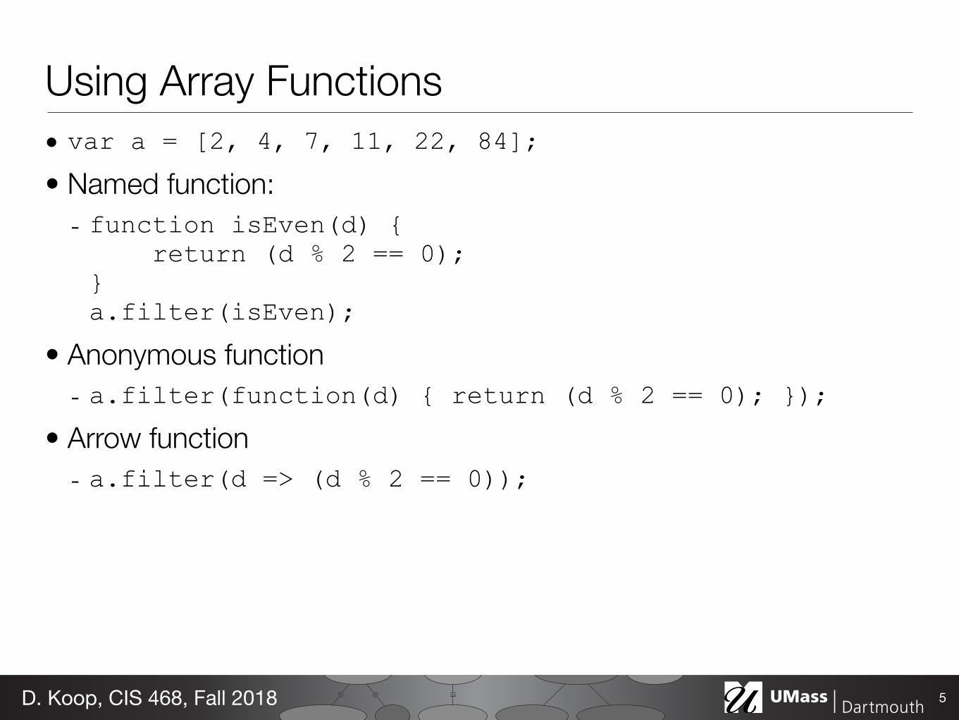

SVG Manipulation Examplebull Draw a horizontal bar chart
- var a = [6 2 6 10 7 18 0 17 20 6] bull Steps
- Programmatically create SVG - Create individual rectangle for each item
10D Koop CIS 468 Fall 2018
Manipulating SVG via JavaScriptbull SVG can be navigated just like the DOM bull Example
function addEltToSVG(svg name attrs) var element = documentcreateElementNS( httpwwww3org2000svg name) if (attrs === undefined) attrs = for (var key in attrs) elementsetAttribute(key attrs[key]) svgappendChild(element) mysvg = documentgetElementById(mysvg) addEltToSVG(mysvg rect x 50 y 50 width 40height 40 fill blue)
11D Koop CIS 468 Fall 2018
SVG Manipulation Examplebull Possible Solution
- httpcodepeniodakooppenGrdBjE
12D Koop CIS 468 Fall 2018
Assignment 1bull httpwwwcisumassdedu
~dkoopcis468-2018faassignment1html
bull Due next Tuesday (Sept 25) bull HTML CSS SVG JavaScript bull Questions
13D Koop CIS 468 Fall 2018
ldquoComputer-based visualization systems provide visual representations of datasets designed to help people carry out tasks more effectivelyrdquo
mdash T Munzner
14D Koop CIS 468 Fall 2018
Databull What is this data
bull Semantics real-world meaning of the data bull Type structural or mathematical interpretation bull Both often require metadata
- Sometimes we can infer some of this information - Line between data and metadata isnrsquot always clear
15D Koop CIS 468 Fall 2018
Data
16D Koop CIS 468 Fall 2018
Data Terminologybull Items
- An item is an individual discrete entity - eg row in a table node in a network
bull Attributes - An attribute is some specific property that can be measured
observed or logged - aka variable (data) dimension - eg a column in a table
17D Koop CIS 468 Fall 2018
Semanticsbull The meaning of the databull Example 94023 90210 52790 02747
18D Koop CIS 468 Fall 2018
Semanticsbull The meaning of the databull Example 94023 90210 52790 02747
- Attendance at college football games
18D Koop CIS 468 Fall 2018
Semanticsbull The meaning of the databull Example 94023 90210 52790 02747
- Attendance at college football games- Salaries
18D Koop CIS 468 Fall 2018
Semanticsbull The meaning of the databull Example 94023 90210 52790 02747
- Attendance at college football games- Salaries- Zip codes
bull Cannot always infer based on what the data looks likebull Often require semantics to better understand databull Column names help with semanticsbull May also include rules about data a zip code is part of an address
that uniquely identifies a residencebull Useful for asking good questions about the data
18D Koop CIS 468 Fall 2018
Items amp Attributes
19
22
Fieldattribute
item
D Koop CIS 468 Fall 2018
Data Typesbull Nodes
- Synonym for item but in the context of networks (graphs) bull Links
- A link is a relation between two items - eg social network friends computer network links
20D Koop CIS 468 Fall 2018
Items amp Links
21
[Bostock 2011]D Koop CIS 468 Fall 2018
Item
Links
Data Typesbull Positions
- A position is a location in space (usually 2D or 3D) - May be subject to projections - eg cities on a map a sampled region in an CT scan
bull Grids - A grid specifies how data is sampled both geometrically and
topologically - eg how CT scan data is stored
22D Koop CIS 468 Fall 2018
Positions and Grids
23D Koop CIS 468 Fall 2018
Position Grid
Dataset Types
24
Tables
Attributes (columns)
Items (rows)
Cell containing value
Networks
Link
Node (item)
Trees
Fields (Continuous)
Attributes (columns)
Value in cell
Cell
Multidimensional Table
Value in cell
Grid of positions
Geometry (Spatial)
Position
Dataset Types
[Munzner (ill Maguire) 2014]D Koop CIS 468 Fall 2018
Tables
25
Fieldattribute
itemcell
D Koop CIS 468 Fall 2018
Attribute SemanticsKeys vs Values (Tables) or Independent vs Dependent (Fields)
Flat
Multidimensional
Tabl
es
Fiel
ds
Tablesbull Data organized by rows amp columns
- row ~ item (usually) - column ~ attribute - label ~ attribute name
bull Key identifies each item (row) - Usually unique - Allows join of data from 2+ tables - Compound key key split among
multiple columns eg (state year) for population
bull Multidimensional - Split compound key - eg a data cube with (state year)
26
[Munzner (ill Maguire) 2014]D Koop CIS 468 Fall 2018
Table Visualizations
27
0
0
0
0
0
0
00
5
5
5
5
5
5
55
10
10
10
10
10
10
1010
15
15
15
15
15
15
1515
20
20
20
20
20
20
2020
25
25
25
25
25
25
2525
30
30
30
30
30
30
3030
35
35
35
35
35
35
3535
40
40
40
40
40
40
4040
45
45
45
45
45
45
4545
economy (mpg)
economy (mpg)
economy (mpg)
economy (mpg)
economy (mpg)
economy (mpg)
economy (mpg)economy (mpg)
30
30
30
30
30
30
3030
35
35
35
35
35
35
3535
40
40
40
40
40
40
4040
45
45
45
45
45
45
4545
50
50
50
50
50
50
5050
55
55
55
55
55
55
5555
60
60
60
60
60
60
6060
65
65
65
65
65
65
6565
70
70
70
70
70
70
7070
75
75
75
75
75
75
7575
80
80
80
80
80
80
8080cylinders
cylinders
cylinders
cylinders
cylinders
cylinders
cylinderscylinders
100
100
100
100
100
100
100100
150
150
150
150
150
150
150150
200
200
200
200
200
200
200200
250
250
250
250
250
250
250250
300
300
300
300
300
300
300300
350
350
350
350
350
350
350350
400
400
400
400
400
400
400400
450
450
450
450
450
450
450450
displacement (cc)
displacement (cc)
displacement (cc)
displacement (cc)
displacement (cc)
displacement (cc)
displacement (cc)displacement (cc)
0
0
0
0
0
0
00
20
20
20
20
20
20
2020
40
40
40
40
40
40
4040
60
60
60
60
60
60
6060
80
80
80
80
80
80
8080
100
100
100
100
100
100
100100
120
120
120
120
120
120
120120
140
140
140
140
140
140
140140
160
160
160
160
160
160
160160
180
180
180
180
180
180
180180
200
200
200
200
200
200
200200
220
220
220
220
220
220
220220
power (hp)
power (hp)
power (hp)
power (hp)
power (hp)
power (hp)
power (hp)power (hp)
2000
2000
2000
2000
2000
2000
20002000
2500
2500
2500
2500
2500
2500
25002500
3000
3000
3000
3000
3000
3000
30003000
3500
3500
3500
3500
3500
3500
35003500
4000
4000
4000
4000
4000
4000
40004000
4500
4500
4500
4500
4500
4500
45004500
5000
5000
5000
5000
5000
5000
50005000
weight (lb)
weight (lb)
weight (lb)
weight (lb)
weight (lb)
weight (lb)
weight (lb)weight (lb)
8
8
8
8
8
8
88
10
10
10
10
10
10
1010
12
12
12
12
12
12
1212
14
14
14
14
14
14
1414
16
16
16
16
16
16
1616
18
18
18
18
18
18
1818
20
20
20
20
20
20
2020
22
22
22
22
22
22
2222
24
24
24
24
24
24
2424
0-60 mph (s)
0-60 mph (s)
0-60 mph (s)
0-60 mph (s)
0-60 mph (s)
0-60 mph (s)
0-60 mph (s)0-60 mph (s)
70
70
70
70
70
70
7070
71
71
71
71
71
71
7171
72
72
72
72
72
72
7272
73
73
73
73
73
73
7373
74
74
74
74
74
74
7474
75
75
75
75
75
75
7575
76
76
76
76
76
76
7676
77
77
77
77
77
77
7777
78
78
78
78
78
78
7878
79
79
79
79
79
79
7979
80
80
80
80
80
80
8080
81
81
81
81
81
81
8181
82
82
82
82
82
82
8282year
year
year
year
year
year
yearyear
[M Bostock 2011]D Koop CIS 468 Fall 2018
Networksbull Why networks instead of graphs bull Tables can represent networks
- Many-many relationships - Also can be stored as specific
graph databases or files
28D Koop CIS 468 Fall 2018
Networks
29
Danny Holten amp Jarke J van Wijk Force-Directed Edge Bundling for Graph Visualization
Figure 7 US airlines graph (235 nodes 2101 edges) (a) not bundled and bundled using (b) FDEB with inverse-linear model(c) GBEB and (d) FDEB with inverse-quadratic model
Figure 8 US migration graph (1715 nodes 9780 edges) (a) not bundled and bundled using (b) FDEB with inverse-linearmodel (c) GBEB and (d) FDEB with inverse-quadratic model The same migration flow is highlighted in each graph
Figure 9 A low amount of straightening provides an indication of the number of edges comprising a bundle by widening thebundle (a) s = 0 (b) s = 10 and (c) s = 40 If s is 0 color more clearly indicates the number of edges comprising a bundle
we generated use the rendering technique described in Sec-tion 41 To facilitate the comparison of migration flow inFigure 8 we use a similar rendering technique as the onethat Cui et al [CZQ08] used to generate Figure 8c
The airlines graph is comprised of 235 nodes and 2101edges It took 19 seconds to calculate the bundled airlinesgraphs (Figures 7b and 7d) using the calculation scheme pre-
sented in Section 33 The migration graph is comprised of1715 nodes and 9780 edges It took 80 seconds to calculatethe bundled migration graphs (Figures 8b and 8d) using thesame calculation scheme All measurements were performedon an Intel Core 2 Duo 266GHz PC running Windows XPwith 2GB of RAM and a GeForce 8800GT graphics cardOur prototype was implemented in Borland Delphi 7
c 2009 The Author(s)Journal compilation c 2009 The Eurographics Association and Blackwell Publishing Ltd
[Holten amp van Wijk 2009]D Koop CIS 468 Fall 2018
Networks
30
[Holten amp van Wijk 2009]D Koop CIS 468 Fall 2018
Danny Holten amp Jarke J van Wijk Force-Directed Edge Bundling for Graph Visualization
Figure 7 US airlines graph (235 nodes 2101 edges) (a) not bundled and bundled using (b) FDEB with inverse-linear model(c) GBEB and (d) FDEB with inverse-quadratic model
Figure 8 US migration graph (1715 nodes 9780 edges) (a) not bundled and bundled using (b) FDEB with inverse-linearmodel (c) GBEB and (d) FDEB with inverse-quadratic model The same migration flow is highlighted in each graph
Figure 9 A low amount of straightening provides an indication of the number of edges comprising a bundle by widening thebundle (a) s = 0 (b) s = 10 and (c) s = 40 If s is 0 color more clearly indicates the number of edges comprising a bundle
we generated use the rendering technique described in Sec-tion 41 To facilitate the comparison of migration flow inFigure 8 we use a similar rendering technique as the onethat Cui et al [CZQ08] used to generate Figure 8c
The airlines graph is comprised of 235 nodes and 2101edges It took 19 seconds to calculate the bundled airlinesgraphs (Figures 7b and 7d) using the calculation scheme pre-
sented in Section 33 The migration graph is comprised of1715 nodes and 9780 edges It took 80 seconds to calculatethe bundled migration graphs (Figures 8b and 8d) using thesame calculation scheme All measurements were performedon an Intel Core 2 Duo 266GHz PC running Windows XPwith 2GB of RAM and a GeForce 8800GT graphics cardOur prototype was implemented in Borland Delphi 7
c 2009 The Author(s)Journal compilation c 2009 The Eurographics Association and Blackwell Publishing Ltd
Fields
31D Koop CIS 468 Fall 2018
Scalar Fields Vector Fields Tensor Fields
Each point in space has an associated
Vector Fields
s0
2
400 01 02
10 11 12
20 21 22
3
5
2
4v0
v1
v2
3
5
Fields
31D Koop CIS 468 Fall 2018
Scalar Fields Vector Fields Tensor Fields(Order-1 Tensor Fields)(Order-0 Tensor Fields) (Order-2+)
Each point in space has an associated
Scalar
Vector Fields
Vector Tensor
Fieldsbull Difference between continuous and discrete values bull Examples temperature pressure density bull Grids necessary to sample continuous data
bull Interpolation ldquohow to show values between the sampled points in ways that do not misleadrdquo
32D Koop CIS 468 Fall 2018
Grids (Meshes)bull Meshes combine positional information (geometry) with
topological information (connectivity)
bull Mesh type can differ substantial depending in the way mesh cells are formed
From Weiskopf Machiraju Moumlllercopy WeiskopfMachirajuMoumlller
Data Structures
bull Grid typesndash Grids differ substantially in the cells (basic
building blocks) they are constructed from and in the way the topological information is given
scattered uniform rectilinear structured unstructured[Weiskopf Machiraju Moumlller]
Spatial Data Example MRI
33
[via Levine 2014]D Koop CIS 468 Fall 2018
Scivis and Infovisbull Two subfields of visualization bull Scivis deals with data where the spatial position is given with data
- Usually continuous data - Often displaying physical phenonema - Techniques like isosurfacing volume rendering vector field vis
bull In Infovis the data has no set spatial representation designer chooses how to visually represent data
bull Also compare background colors of visualizations )
34D Koop CIS 468 Fall 2018
SciVis
35
[Google Image Search for scientific visualization 2017]D Koop CIS 468 Fall 2018
InfoVis
36
[Google Image Search for information visualization 2017]D Koop CIS 468 Fall 2018
Sets amp Lists
37
[Daniels httpexperimentsundercurrentcom]D Koop CIS 468 Fall 2018
Attribute Types
38
Attributes
Attribute Types
Ordering Direction
Categorical Ordered
Ordinal Quantitative
Sequential Diverging Cyclic
[Munzner (ill Maguire) 2014]D Koop CIS 468 Fall 2018
Categorial Ordinal and Quantitative
39
231 = Quantitative2 = Nominal3 = Ordinal
quantitative ordinal categorical
D Koop CIS 468 Fall 2018
Categorial Ordinal and Quantitative
40
241 = Quantitative2 = Nominal3 = Ordinal
quantitative ordinal categorical
D Koop CIS 468 Fall 2018
Ordering Direction
41
Attributes
Attribute Types
Ordering Direction
Categorical Ordered
Ordinal Quantitative
Sequential Diverging Cyclic
[Munzner (ill Maguire) 2014]D Koop CIS 468 Fall 2018
Sequential and Diverging Databull Sequential homogenous range
from a minimum to a maximum - Examples Land elevations ocean
depths bull Diverging can be deconstructed
into two sequences pointing in opposite directions - Has a zero point (not necessary 0) - Example Map of both land
elevation and ocean depth
42
[Rogowitz amp Treinish 1998]D Koop CIS 468 Fall 2018
Cyclic Data
43
lar structure of spirals allows for an easy detection of cyclesand for the comparison of periodic data sets Furthermorethe continuity of the data is expressed by using a spiral in-stead of a circle
31 Mathematical description and types of spirals
A spiral is easy to describe and understand in polar coor-dinates ie in the form The distinctive feature ofa spiral is that f is a monotone function In this work we as-sume a spiral is described by
Several simple functions f lead to well-known types ofspirals bull Archimedeslsquo spiral has the form It has the spe-
cial property that a ray emanating from the origincrosses two consecutive arcs of the spiral in a constantdistance
bull The Hyperbolic spiral has the form It is theinverse of Archimedeslsquo spiral with respect to the origin
bull More generally spirals of the form are calledArchimedean spirals
bull The logarithmic spiral has the form It has thespecial property that all arcs cut a ray emanating fromthe origin under the same angleFor the visualization of time-dependent data Archimedeslsquo
spiral seems to be the most appropriate In most applicationsdata from different periods are equally important Thisshould be reflected visually in that the distance to other peri-ods is always the same
32 Mapping data to the spiral
In general markers bars and line elements can be usedto visualize time-series data similar to standard point barand line graphs on Spiral Graphs For instance quantitativediscrete data can be presented as bars on the spiral or bymarks with a corresponding distance to the spiral Howeversince the x and y coordinate are needed to achieve the generalform of the spiral their use is limited for the display of datavalues One might consider to map data values to small ab-solute changes in the radius ie
Yet we have found this way of visualizing to be ineffec-tive We conclude that the general shape of the spiral shouldbe untouched and other attributes should be used such asbull colourbull texture including line styles and patterns
Figure 1Two visualizations of sunshine intensity using about the same screen real estate and thesame color coding scheme In the spiral visualization it is much easier to compare days to spotcloudy time periods or to see events like sunrise and sunset
r f ϕ( )=
r f ϕ( ) dfdϕ------ 0 ϕ R+isingt=
r aϕ=
2πar a ϕfrasl=
r aϕk=
r aekϕ=
r aϕ bv ϕ( ) b πamax v ϕ( )( )---------------------------lt+=
[Sunlight intensity Weber et al 2001]D Koop CIS 468 Fall 2018
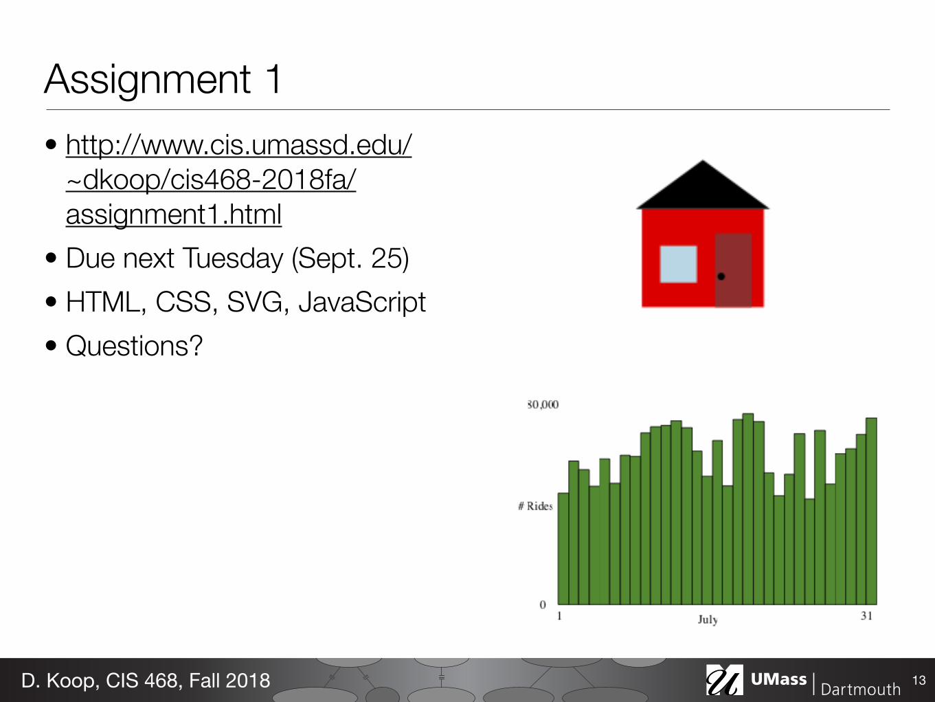
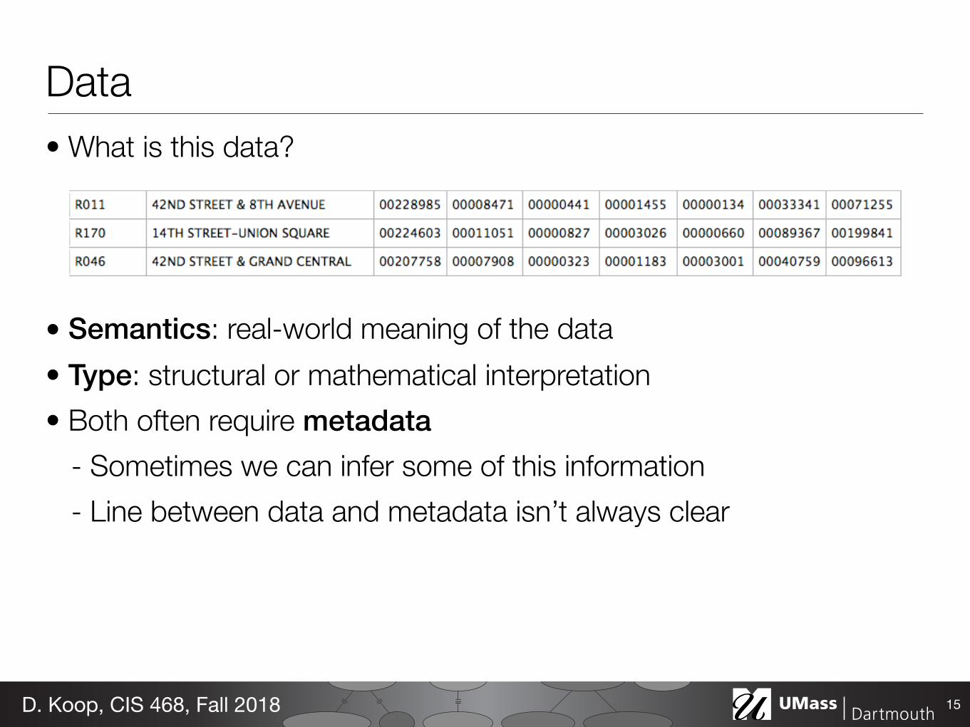

Semanticsbull The meaning of the databull Example 94023 90210 52790 02747
18D Koop CIS 468 Fall 2018
Semanticsbull The meaning of the databull Example 94023 90210 52790 02747
- Attendance at college football games
18D Koop CIS 468 Fall 2018
Semanticsbull The meaning of the databull Example 94023 90210 52790 02747
- Attendance at college football games- Salaries
18D Koop CIS 468 Fall 2018
Semanticsbull The meaning of the databull Example 94023 90210 52790 02747
- Attendance at college football games- Salaries- Zip codes
bull Cannot always infer based on what the data looks likebull Often require semantics to better understand databull Column names help with semanticsbull May also include rules about data a zip code is part of an address
that uniquely identifies a residencebull Useful for asking good questions about the data
18D Koop CIS 468 Fall 2018
Items amp Attributes
19
22
Fieldattribute
item
D Koop CIS 468 Fall 2018
Data Typesbull Nodes
- Synonym for item but in the context of networks (graphs) bull Links
- A link is a relation between two items - eg social network friends computer network links
20D Koop CIS 468 Fall 2018
Items amp Links
21
[Bostock 2011]D Koop CIS 468 Fall 2018
Item
Links
Data Typesbull Positions
- A position is a location in space (usually 2D or 3D) - May be subject to projections - eg cities on a map a sampled region in an CT scan
bull Grids - A grid specifies how data is sampled both geometrically and
topologically - eg how CT scan data is stored
22D Koop CIS 468 Fall 2018
Positions and Grids
23D Koop CIS 468 Fall 2018
Position Grid
Dataset Types
24
Tables
Attributes (columns)
Items (rows)
Cell containing value
Networks
Link
Node (item)
Trees
Fields (Continuous)
Attributes (columns)
Value in cell
Cell
Multidimensional Table
Value in cell
Grid of positions
Geometry (Spatial)
Position
Dataset Types
[Munzner (ill Maguire) 2014]D Koop CIS 468 Fall 2018
Tables
25
Fieldattribute
itemcell
D Koop CIS 468 Fall 2018
Attribute SemanticsKeys vs Values (Tables) or Independent vs Dependent (Fields)
Flat
Multidimensional
Tabl
es
Fiel
ds
Tablesbull Data organized by rows amp columns
- row ~ item (usually) - column ~ attribute - label ~ attribute name
bull Key identifies each item (row) - Usually unique - Allows join of data from 2+ tables - Compound key key split among
multiple columns eg (state year) for population
bull Multidimensional - Split compound key - eg a data cube with (state year)
26
[Munzner (ill Maguire) 2014]D Koop CIS 468 Fall 2018
Table Visualizations
27
0
0
0
0
0
0
00
5
5
5
5
5
5
55
10
10
10
10
10
10
1010
15
15
15
15
15
15
1515
20
20
20
20
20
20
2020
25
25
25
25
25
25
2525
30
30
30
30
30
30
3030
35
35
35
35
35
35
3535
40
40
40
40
40
40
4040
45
45
45
45
45
45
4545
economy (mpg)
economy (mpg)
economy (mpg)
economy (mpg)
economy (mpg)
economy (mpg)
economy (mpg)economy (mpg)
30
30
30
30
30
30
3030
35
35
35
35
35
35
3535
40
40
40
40
40
40
4040
45
45
45
45
45
45
4545
50
50
50
50
50
50
5050
55
55
55
55
55
55
5555
60
60
60
60
60
60
6060
65
65
65
65
65
65
6565
70
70
70
70
70
70
7070
75
75
75
75
75
75
7575
80
80
80
80
80
80
8080cylinders
cylinders
cylinders
cylinders
cylinders
cylinders
cylinderscylinders
100
100
100
100
100
100
100100
150
150
150
150
150
150
150150
200
200
200
200
200
200
200200
250
250
250
250
250
250
250250
300
300
300
300
300
300
300300
350
350
350
350
350
350
350350
400
400
400
400
400
400
400400
450
450
450
450
450
450
450450
displacement (cc)
displacement (cc)
displacement (cc)
displacement (cc)
displacement (cc)
displacement (cc)
displacement (cc)displacement (cc)
0
0
0
0
0
0
00
20
20
20
20
20
20
2020
40
40
40
40
40
40
4040
60
60
60
60
60
60
6060
80
80
80
80
80
80
8080
100
100
100
100
100
100
100100
120
120
120
120
120
120
120120
140
140
140
140
140
140
140140
160
160
160
160
160
160
160160
180
180
180
180
180
180
180180
200
200
200
200
200
200
200200
220
220
220
220
220
220
220220
power (hp)
power (hp)
power (hp)
power (hp)
power (hp)
power (hp)
power (hp)power (hp)
2000
2000
2000
2000
2000
2000
20002000
2500
2500
2500
2500
2500
2500
25002500
3000
3000
3000
3000
3000
3000
30003000
3500
3500
3500
3500
3500
3500
35003500
4000
4000
4000
4000
4000
4000
40004000
4500
4500
4500
4500
4500
4500
45004500
5000
5000
5000
5000
5000
5000
50005000
weight (lb)
weight (lb)
weight (lb)
weight (lb)
weight (lb)
weight (lb)
weight (lb)weight (lb)
8
8
8
8
8
8
88
10
10
10
10
10
10
1010
12
12
12
12
12
12
1212
14
14
14
14
14
14
1414
16
16
16
16
16
16
1616
18
18
18
18
18
18
1818
20
20
20
20
20
20
2020
22
22
22
22
22
22
2222
24
24
24
24
24
24
2424
0-60 mph (s)
0-60 mph (s)
0-60 mph (s)
0-60 mph (s)
0-60 mph (s)
0-60 mph (s)
0-60 mph (s)0-60 mph (s)
70
70
70
70
70
70
7070
71
71
71
71
71
71
7171
72
72
72
72
72
72
7272
73
73
73
73
73
73
7373
74
74
74
74
74
74
7474
75
75
75
75
75
75
7575
76
76
76
76
76
76
7676
77
77
77
77
77
77
7777
78
78
78
78
78
78
7878
79
79
79
79
79
79
7979
80
80
80
80
80
80
8080
81
81
81
81
81
81
8181
82
82
82
82
82
82
8282year
year
year
year
year
year
yearyear
[M Bostock 2011]D Koop CIS 468 Fall 2018
Networksbull Why networks instead of graphs bull Tables can represent networks
- Many-many relationships - Also can be stored as specific
graph databases or files
28D Koop CIS 468 Fall 2018
Networks
29
Danny Holten amp Jarke J van Wijk Force-Directed Edge Bundling for Graph Visualization
Figure 7 US airlines graph (235 nodes 2101 edges) (a) not bundled and bundled using (b) FDEB with inverse-linear model(c) GBEB and (d) FDEB with inverse-quadratic model
Figure 8 US migration graph (1715 nodes 9780 edges) (a) not bundled and bundled using (b) FDEB with inverse-linearmodel (c) GBEB and (d) FDEB with inverse-quadratic model The same migration flow is highlighted in each graph
Figure 9 A low amount of straightening provides an indication of the number of edges comprising a bundle by widening thebundle (a) s = 0 (b) s = 10 and (c) s = 40 If s is 0 color more clearly indicates the number of edges comprising a bundle
we generated use the rendering technique described in Sec-tion 41 To facilitate the comparison of migration flow inFigure 8 we use a similar rendering technique as the onethat Cui et al [CZQ08] used to generate Figure 8c
The airlines graph is comprised of 235 nodes and 2101edges It took 19 seconds to calculate the bundled airlinesgraphs (Figures 7b and 7d) using the calculation scheme pre-
sented in Section 33 The migration graph is comprised of1715 nodes and 9780 edges It took 80 seconds to calculatethe bundled migration graphs (Figures 8b and 8d) using thesame calculation scheme All measurements were performedon an Intel Core 2 Duo 266GHz PC running Windows XPwith 2GB of RAM and a GeForce 8800GT graphics cardOur prototype was implemented in Borland Delphi 7
c 2009 The Author(s)Journal compilation c 2009 The Eurographics Association and Blackwell Publishing Ltd
[Holten amp van Wijk 2009]D Koop CIS 468 Fall 2018
Networks
30
[Holten amp van Wijk 2009]D Koop CIS 468 Fall 2018
Danny Holten amp Jarke J van Wijk Force-Directed Edge Bundling for Graph Visualization
Figure 7 US airlines graph (235 nodes 2101 edges) (a) not bundled and bundled using (b) FDEB with inverse-linear model(c) GBEB and (d) FDEB with inverse-quadratic model
Figure 8 US migration graph (1715 nodes 9780 edges) (a) not bundled and bundled using (b) FDEB with inverse-linearmodel (c) GBEB and (d) FDEB with inverse-quadratic model The same migration flow is highlighted in each graph
Figure 9 A low amount of straightening provides an indication of the number of edges comprising a bundle by widening thebundle (a) s = 0 (b) s = 10 and (c) s = 40 If s is 0 color more clearly indicates the number of edges comprising a bundle
we generated use the rendering technique described in Sec-tion 41 To facilitate the comparison of migration flow inFigure 8 we use a similar rendering technique as the onethat Cui et al [CZQ08] used to generate Figure 8c
The airlines graph is comprised of 235 nodes and 2101edges It took 19 seconds to calculate the bundled airlinesgraphs (Figures 7b and 7d) using the calculation scheme pre-
sented in Section 33 The migration graph is comprised of1715 nodes and 9780 edges It took 80 seconds to calculatethe bundled migration graphs (Figures 8b and 8d) using thesame calculation scheme All measurements were performedon an Intel Core 2 Duo 266GHz PC running Windows XPwith 2GB of RAM and a GeForce 8800GT graphics cardOur prototype was implemented in Borland Delphi 7
c 2009 The Author(s)Journal compilation c 2009 The Eurographics Association and Blackwell Publishing Ltd
Fields
31D Koop CIS 468 Fall 2018
Scalar Fields Vector Fields Tensor Fields
Each point in space has an associated
Vector Fields
s0
2
400 01 02
10 11 12
20 21 22
3
5
2
4v0
v1
v2
3
5
Fields
31D Koop CIS 468 Fall 2018
Scalar Fields Vector Fields Tensor Fields(Order-1 Tensor Fields)(Order-0 Tensor Fields) (Order-2+)
Each point in space has an associated
Scalar
Vector Fields
Vector Tensor
Fieldsbull Difference between continuous and discrete values bull Examples temperature pressure density bull Grids necessary to sample continuous data
bull Interpolation ldquohow to show values between the sampled points in ways that do not misleadrdquo
32D Koop CIS 468 Fall 2018
Grids (Meshes)bull Meshes combine positional information (geometry) with
topological information (connectivity)
bull Mesh type can differ substantial depending in the way mesh cells are formed
From Weiskopf Machiraju Moumlllercopy WeiskopfMachirajuMoumlller
Data Structures
bull Grid typesndash Grids differ substantially in the cells (basic
building blocks) they are constructed from and in the way the topological information is given
scattered uniform rectilinear structured unstructured[Weiskopf Machiraju Moumlller]
Spatial Data Example MRI
33
[via Levine 2014]D Koop CIS 468 Fall 2018
Scivis and Infovisbull Two subfields of visualization bull Scivis deals with data where the spatial position is given with data
- Usually continuous data - Often displaying physical phenonema - Techniques like isosurfacing volume rendering vector field vis
bull In Infovis the data has no set spatial representation designer chooses how to visually represent data
bull Also compare background colors of visualizations )
34D Koop CIS 468 Fall 2018
SciVis
35
[Google Image Search for scientific visualization 2017]D Koop CIS 468 Fall 2018
InfoVis
36
[Google Image Search for information visualization 2017]D Koop CIS 468 Fall 2018
Sets amp Lists
37
[Daniels httpexperimentsundercurrentcom]D Koop CIS 468 Fall 2018
Attribute Types
38
Attributes
Attribute Types
Ordering Direction
Categorical Ordered
Ordinal Quantitative
Sequential Diverging Cyclic
[Munzner (ill Maguire) 2014]D Koop CIS 468 Fall 2018
Categorial Ordinal and Quantitative
39
231 = Quantitative2 = Nominal3 = Ordinal
quantitative ordinal categorical
D Koop CIS 468 Fall 2018
Categorial Ordinal and Quantitative
40
241 = Quantitative2 = Nominal3 = Ordinal
quantitative ordinal categorical
D Koop CIS 468 Fall 2018
Ordering Direction
41
Attributes
Attribute Types
Ordering Direction
Categorical Ordered
Ordinal Quantitative
Sequential Diverging Cyclic
[Munzner (ill Maguire) 2014]D Koop CIS 468 Fall 2018
Sequential and Diverging Databull Sequential homogenous range
from a minimum to a maximum - Examples Land elevations ocean
depths bull Diverging can be deconstructed
into two sequences pointing in opposite directions - Has a zero point (not necessary 0) - Example Map of both land
elevation and ocean depth
42
[Rogowitz amp Treinish 1998]D Koop CIS 468 Fall 2018
Cyclic Data
43
lar structure of spirals allows for an easy detection of cyclesand for the comparison of periodic data sets Furthermorethe continuity of the data is expressed by using a spiral in-stead of a circle
31 Mathematical description and types of spirals
A spiral is easy to describe and understand in polar coor-dinates ie in the form The distinctive feature ofa spiral is that f is a monotone function In this work we as-sume a spiral is described by
Several simple functions f lead to well-known types ofspirals bull Archimedeslsquo spiral has the form It has the spe-
cial property that a ray emanating from the origincrosses two consecutive arcs of the spiral in a constantdistance
bull The Hyperbolic spiral has the form It is theinverse of Archimedeslsquo spiral with respect to the origin
bull More generally spirals of the form are calledArchimedean spirals
bull The logarithmic spiral has the form It has thespecial property that all arcs cut a ray emanating fromthe origin under the same angleFor the visualization of time-dependent data Archimedeslsquo
spiral seems to be the most appropriate In most applicationsdata from different periods are equally important Thisshould be reflected visually in that the distance to other peri-ods is always the same
32 Mapping data to the spiral
In general markers bars and line elements can be usedto visualize time-series data similar to standard point barand line graphs on Spiral Graphs For instance quantitativediscrete data can be presented as bars on the spiral or bymarks with a corresponding distance to the spiral Howeversince the x and y coordinate are needed to achieve the generalform of the spiral their use is limited for the display of datavalues One might consider to map data values to small ab-solute changes in the radius ie
Yet we have found this way of visualizing to be ineffec-tive We conclude that the general shape of the spiral shouldbe untouched and other attributes should be used such asbull colourbull texture including line styles and patterns
Figure 1Two visualizations of sunshine intensity using about the same screen real estate and thesame color coding scheme In the spiral visualization it is much easier to compare days to spotcloudy time periods or to see events like sunrise and sunset
r f ϕ( )=
r f ϕ( ) dfdϕ------ 0 ϕ R+isingt=
r aϕ=
2πar a ϕfrasl=
r aϕk=
r aekϕ=
r aϕ bv ϕ( ) b πamax v ϕ( )( )---------------------------lt+=
[Sunlight intensity Weber et al 2001]D Koop CIS 468 Fall 2018
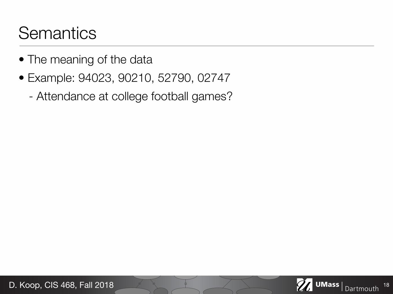
Semanticsbull The meaning of the databull Example 94023 90210 52790 02747
- Attendance at college football games
18D Koop CIS 468 Fall 2018
Semanticsbull The meaning of the databull Example 94023 90210 52790 02747
- Attendance at college football games- Salaries
18D Koop CIS 468 Fall 2018
Semanticsbull The meaning of the databull Example 94023 90210 52790 02747
- Attendance at college football games- Salaries- Zip codes
bull Cannot always infer based on what the data looks likebull Often require semantics to better understand databull Column names help with semanticsbull May also include rules about data a zip code is part of an address
that uniquely identifies a residencebull Useful for asking good questions about the data
18D Koop CIS 468 Fall 2018
Items amp Attributes
19
22
Fieldattribute
item
D Koop CIS 468 Fall 2018
Data Typesbull Nodes
- Synonym for item but in the context of networks (graphs) bull Links
- A link is a relation between two items - eg social network friends computer network links
20D Koop CIS 468 Fall 2018
Items amp Links
21
[Bostock 2011]D Koop CIS 468 Fall 2018
Item
Links
Data Typesbull Positions
- A position is a location in space (usually 2D or 3D) - May be subject to projections - eg cities on a map a sampled region in an CT scan
bull Grids - A grid specifies how data is sampled both geometrically and
topologically - eg how CT scan data is stored
22D Koop CIS 468 Fall 2018
Positions and Grids
23D Koop CIS 468 Fall 2018
Position Grid
Dataset Types
24
Tables
Attributes (columns)
Items (rows)
Cell containing value
Networks
Link
Node (item)
Trees
Fields (Continuous)
Attributes (columns)
Value in cell
Cell
Multidimensional Table
Value in cell
Grid of positions
Geometry (Spatial)
Position
Dataset Types
[Munzner (ill Maguire) 2014]D Koop CIS 468 Fall 2018
Tables
25
Fieldattribute
itemcell
D Koop CIS 468 Fall 2018
Attribute SemanticsKeys vs Values (Tables) or Independent vs Dependent (Fields)
Flat
Multidimensional
Tabl
es
Fiel
ds
Tablesbull Data organized by rows amp columns
- row ~ item (usually) - column ~ attribute - label ~ attribute name
bull Key identifies each item (row) - Usually unique - Allows join of data from 2+ tables - Compound key key split among
multiple columns eg (state year) for population
bull Multidimensional - Split compound key - eg a data cube with (state year)
26
[Munzner (ill Maguire) 2014]D Koop CIS 468 Fall 2018
Table Visualizations
27
0
0
0
0
0
0
00
5
5
5
5
5
5
55
10
10
10
10
10
10
1010
15
15
15
15
15
15
1515
20
20
20
20
20
20
2020
25
25
25
25
25
25
2525
30
30
30
30
30
30
3030
35
35
35
35
35
35
3535
40
40
40
40
40
40
4040
45
45
45
45
45
45
4545
economy (mpg)
economy (mpg)
economy (mpg)
economy (mpg)
economy (mpg)
economy (mpg)
economy (mpg)economy (mpg)
30
30
30
30
30
30
3030
35
35
35
35
35
35
3535
40
40
40
40
40
40
4040
45
45
45
45
45
45
4545
50
50
50
50
50
50
5050
55
55
55
55
55
55
5555
60
60
60
60
60
60
6060
65
65
65
65
65
65
6565
70
70
70
70
70
70
7070
75
75
75
75
75
75
7575
80
80
80
80
80
80
8080cylinders
cylinders
cylinders
cylinders
cylinders
cylinders
cylinderscylinders
100
100
100
100
100
100
100100
150
150
150
150
150
150
150150
200
200
200
200
200
200
200200
250
250
250
250
250
250
250250
300
300
300
300
300
300
300300
350
350
350
350
350
350
350350
400
400
400
400
400
400
400400
450
450
450
450
450
450
450450
displacement (cc)
displacement (cc)
displacement (cc)
displacement (cc)
displacement (cc)
displacement (cc)
displacement (cc)displacement (cc)
0
0
0
0
0
0
00
20
20
20
20
20
20
2020
40
40
40
40
40
40
4040
60
60
60
60
60
60
6060
80
80
80
80
80
80
8080
100
100
100
100
100
100
100100
120
120
120
120
120
120
120120
140
140
140
140
140
140
140140
160
160
160
160
160
160
160160
180
180
180
180
180
180
180180
200
200
200
200
200
200
200200
220
220
220
220
220
220
220220
power (hp)
power (hp)
power (hp)
power (hp)
power (hp)
power (hp)
power (hp)power (hp)
2000
2000
2000
2000
2000
2000
20002000
2500
2500
2500
2500
2500
2500
25002500
3000
3000
3000
3000
3000
3000
30003000
3500
3500
3500
3500
3500
3500
35003500
4000
4000
4000
4000
4000
4000
40004000
4500
4500
4500
4500
4500
4500
45004500
5000
5000
5000
5000
5000
5000
50005000
weight (lb)
weight (lb)
weight (lb)
weight (lb)
weight (lb)
weight (lb)
weight (lb)weight (lb)
8
8
8
8
8
8
88
10
10
10
10
10
10
1010
12
12
12
12
12
12
1212
14
14
14
14
14
14
1414
16
16
16
16
16
16
1616
18
18
18
18
18
18
1818
20
20
20
20
20
20
2020
22
22
22
22
22
22
2222
24
24
24
24
24
24
2424
0-60 mph (s)
0-60 mph (s)
0-60 mph (s)
0-60 mph (s)
0-60 mph (s)
0-60 mph (s)
0-60 mph (s)0-60 mph (s)
70
70
70
70
70
70
7070
71
71
71
71
71
71
7171
72
72
72
72
72
72
7272
73
73
73
73
73
73
7373
74
74
74
74
74
74
7474
75
75
75
75
75
75
7575
76
76
76
76
76
76
7676
77
77
77
77
77
77
7777
78
78
78
78
78
78
7878
79
79
79
79
79
79
7979
80
80
80
80
80
80
8080
81
81
81
81
81
81
8181
82
82
82
82
82
82
8282year
year
year
year
year
year
yearyear
[M Bostock 2011]D Koop CIS 468 Fall 2018
Networksbull Why networks instead of graphs bull Tables can represent networks
- Many-many relationships - Also can be stored as specific
graph databases or files
28D Koop CIS 468 Fall 2018
Networks
29
Danny Holten amp Jarke J van Wijk Force-Directed Edge Bundling for Graph Visualization
Figure 7 US airlines graph (235 nodes 2101 edges) (a) not bundled and bundled using (b) FDEB with inverse-linear model(c) GBEB and (d) FDEB with inverse-quadratic model
Figure 8 US migration graph (1715 nodes 9780 edges) (a) not bundled and bundled using (b) FDEB with inverse-linearmodel (c) GBEB and (d) FDEB with inverse-quadratic model The same migration flow is highlighted in each graph
Figure 9 A low amount of straightening provides an indication of the number of edges comprising a bundle by widening thebundle (a) s = 0 (b) s = 10 and (c) s = 40 If s is 0 color more clearly indicates the number of edges comprising a bundle
we generated use the rendering technique described in Sec-tion 41 To facilitate the comparison of migration flow inFigure 8 we use a similar rendering technique as the onethat Cui et al [CZQ08] used to generate Figure 8c
The airlines graph is comprised of 235 nodes and 2101edges It took 19 seconds to calculate the bundled airlinesgraphs (Figures 7b and 7d) using the calculation scheme pre-
sented in Section 33 The migration graph is comprised of1715 nodes and 9780 edges It took 80 seconds to calculatethe bundled migration graphs (Figures 8b and 8d) using thesame calculation scheme All measurements were performedon an Intel Core 2 Duo 266GHz PC running Windows XPwith 2GB of RAM and a GeForce 8800GT graphics cardOur prototype was implemented in Borland Delphi 7
c 2009 The Author(s)Journal compilation c 2009 The Eurographics Association and Blackwell Publishing Ltd
[Holten amp van Wijk 2009]D Koop CIS 468 Fall 2018
Networks
30
[Holten amp van Wijk 2009]D Koop CIS 468 Fall 2018
Danny Holten amp Jarke J van Wijk Force-Directed Edge Bundling for Graph Visualization
Figure 7 US airlines graph (235 nodes 2101 edges) (a) not bundled and bundled using (b) FDEB with inverse-linear model(c) GBEB and (d) FDEB with inverse-quadratic model
Figure 8 US migration graph (1715 nodes 9780 edges) (a) not bundled and bundled using (b) FDEB with inverse-linearmodel (c) GBEB and (d) FDEB with inverse-quadratic model The same migration flow is highlighted in each graph
Figure 9 A low amount of straightening provides an indication of the number of edges comprising a bundle by widening thebundle (a) s = 0 (b) s = 10 and (c) s = 40 If s is 0 color more clearly indicates the number of edges comprising a bundle
we generated use the rendering technique described in Sec-tion 41 To facilitate the comparison of migration flow inFigure 8 we use a similar rendering technique as the onethat Cui et al [CZQ08] used to generate Figure 8c
The airlines graph is comprised of 235 nodes and 2101edges It took 19 seconds to calculate the bundled airlinesgraphs (Figures 7b and 7d) using the calculation scheme pre-
sented in Section 33 The migration graph is comprised of1715 nodes and 9780 edges It took 80 seconds to calculatethe bundled migration graphs (Figures 8b and 8d) using thesame calculation scheme All measurements were performedon an Intel Core 2 Duo 266GHz PC running Windows XPwith 2GB of RAM and a GeForce 8800GT graphics cardOur prototype was implemented in Borland Delphi 7
c 2009 The Author(s)Journal compilation c 2009 The Eurographics Association and Blackwell Publishing Ltd
Fields
31D Koop CIS 468 Fall 2018
Scalar Fields Vector Fields Tensor Fields
Each point in space has an associated
Vector Fields
s0
2
400 01 02
10 11 12
20 21 22
3
5
2
4v0
v1
v2
3
5
Fields
31D Koop CIS 468 Fall 2018
Scalar Fields Vector Fields Tensor Fields(Order-1 Tensor Fields)(Order-0 Tensor Fields) (Order-2+)
Each point in space has an associated
Scalar
Vector Fields
Vector Tensor
Fieldsbull Difference between continuous and discrete values bull Examples temperature pressure density bull Grids necessary to sample continuous data
bull Interpolation ldquohow to show values between the sampled points in ways that do not misleadrdquo
32D Koop CIS 468 Fall 2018
Grids (Meshes)bull Meshes combine positional information (geometry) with
topological information (connectivity)
bull Mesh type can differ substantial depending in the way mesh cells are formed
From Weiskopf Machiraju Moumlllercopy WeiskopfMachirajuMoumlller
Data Structures
bull Grid typesndash Grids differ substantially in the cells (basic
building blocks) they are constructed from and in the way the topological information is given
scattered uniform rectilinear structured unstructured[Weiskopf Machiraju Moumlller]
Spatial Data Example MRI
33
[via Levine 2014]D Koop CIS 468 Fall 2018
Scivis and Infovisbull Two subfields of visualization bull Scivis deals with data where the spatial position is given with data
- Usually continuous data - Often displaying physical phenonema - Techniques like isosurfacing volume rendering vector field vis
bull In Infovis the data has no set spatial representation designer chooses how to visually represent data
bull Also compare background colors of visualizations )
34D Koop CIS 468 Fall 2018
SciVis
35
[Google Image Search for scientific visualization 2017]D Koop CIS 468 Fall 2018
InfoVis
36
[Google Image Search for information visualization 2017]D Koop CIS 468 Fall 2018
Sets amp Lists
37
[Daniels httpexperimentsundercurrentcom]D Koop CIS 468 Fall 2018
Attribute Types
38
Attributes
Attribute Types
Ordering Direction
Categorical Ordered
Ordinal Quantitative
Sequential Diverging Cyclic
[Munzner (ill Maguire) 2014]D Koop CIS 468 Fall 2018
Categorial Ordinal and Quantitative
39
231 = Quantitative2 = Nominal3 = Ordinal
quantitative ordinal categorical
D Koop CIS 468 Fall 2018
Categorial Ordinal and Quantitative
40
241 = Quantitative2 = Nominal3 = Ordinal
quantitative ordinal categorical
D Koop CIS 468 Fall 2018
Ordering Direction
41
Attributes
Attribute Types
Ordering Direction
Categorical Ordered
Ordinal Quantitative
Sequential Diverging Cyclic
[Munzner (ill Maguire) 2014]D Koop CIS 468 Fall 2018
Sequential and Diverging Databull Sequential homogenous range
from a minimum to a maximum - Examples Land elevations ocean
depths bull Diverging can be deconstructed
into two sequences pointing in opposite directions - Has a zero point (not necessary 0) - Example Map of both land
elevation and ocean depth
42
[Rogowitz amp Treinish 1998]D Koop CIS 468 Fall 2018
Cyclic Data
43
lar structure of spirals allows for an easy detection of cyclesand for the comparison of periodic data sets Furthermorethe continuity of the data is expressed by using a spiral in-stead of a circle
31 Mathematical description and types of spirals
A spiral is easy to describe and understand in polar coor-dinates ie in the form The distinctive feature ofa spiral is that f is a monotone function In this work we as-sume a spiral is described by
Several simple functions f lead to well-known types ofspirals bull Archimedeslsquo spiral has the form It has the spe-
cial property that a ray emanating from the origincrosses two consecutive arcs of the spiral in a constantdistance
bull The Hyperbolic spiral has the form It is theinverse of Archimedeslsquo spiral with respect to the origin
bull More generally spirals of the form are calledArchimedean spirals
bull The logarithmic spiral has the form It has thespecial property that all arcs cut a ray emanating fromthe origin under the same angleFor the visualization of time-dependent data Archimedeslsquo
spiral seems to be the most appropriate In most applicationsdata from different periods are equally important Thisshould be reflected visually in that the distance to other peri-ods is always the same
32 Mapping data to the spiral
In general markers bars and line elements can be usedto visualize time-series data similar to standard point barand line graphs on Spiral Graphs For instance quantitativediscrete data can be presented as bars on the spiral or bymarks with a corresponding distance to the spiral Howeversince the x and y coordinate are needed to achieve the generalform of the spiral their use is limited for the display of datavalues One might consider to map data values to small ab-solute changes in the radius ie
Yet we have found this way of visualizing to be ineffec-tive We conclude that the general shape of the spiral shouldbe untouched and other attributes should be used such asbull colourbull texture including line styles and patterns
Figure 1Two visualizations of sunshine intensity using about the same screen real estate and thesame color coding scheme In the spiral visualization it is much easier to compare days to spotcloudy time periods or to see events like sunrise and sunset
r f ϕ( )=
r f ϕ( ) dfdϕ------ 0 ϕ R+isingt=
r aϕ=
2πar a ϕfrasl=
r aϕk=
r aekϕ=
r aϕ bv ϕ( ) b πamax v ϕ( )( )---------------------------lt+=
[Sunlight intensity Weber et al 2001]D Koop CIS 468 Fall 2018
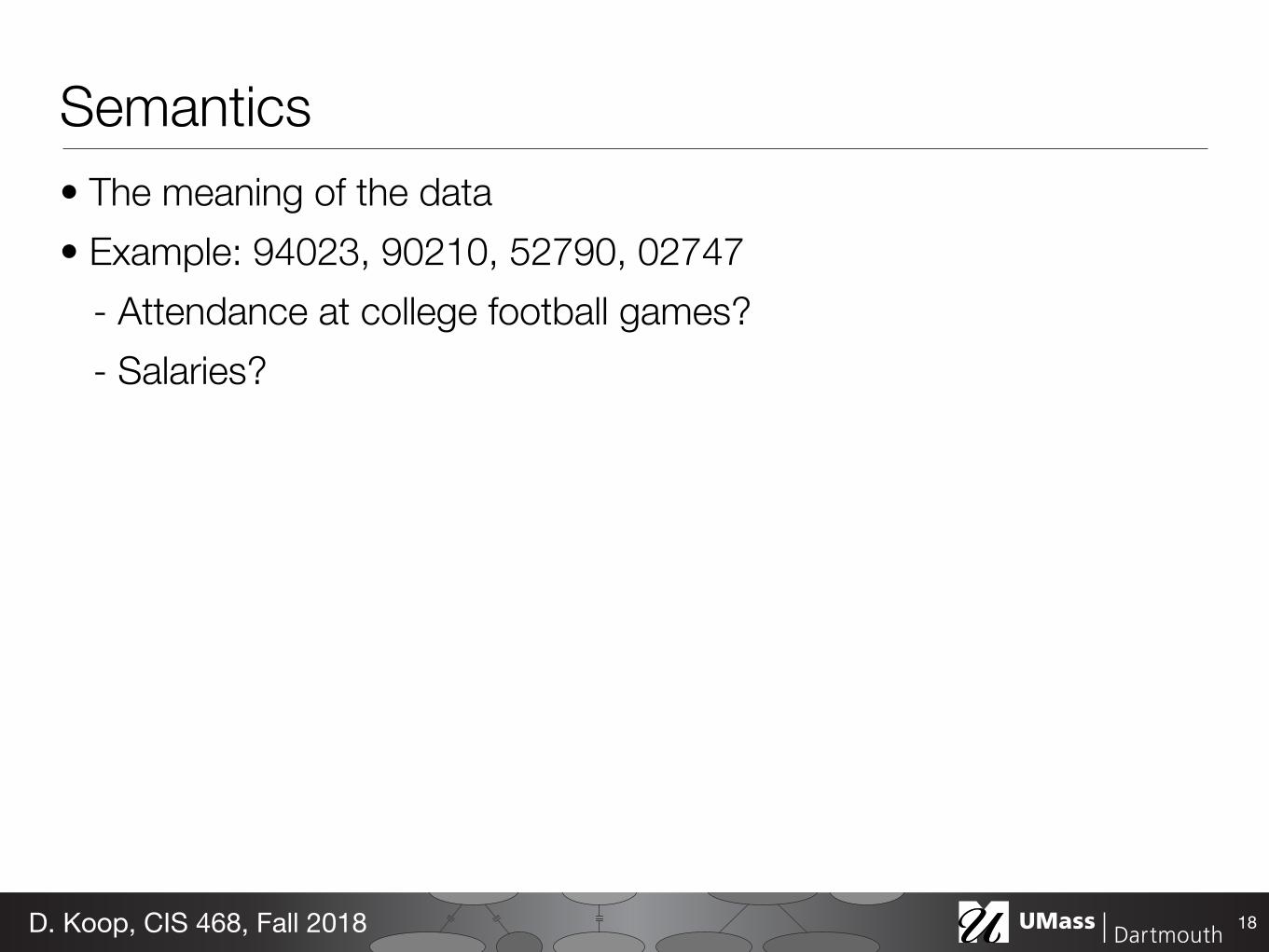
Semanticsbull The meaning of the databull Example 94023 90210 52790 02747
- Attendance at college football games- Salaries- Zip codes
bull Cannot always infer based on what the data looks likebull Often require semantics to better understand databull Column names help with semanticsbull May also include rules about data a zip code is part of an address
that uniquely identifies a residencebull Useful for asking good questions about the data
18D Koop CIS 468 Fall 2018
Items amp Attributes
19
22
Fieldattribute
item
D Koop CIS 468 Fall 2018
Data Typesbull Nodes
- Synonym for item but in the context of networks (graphs) bull Links
- A link is a relation between two items - eg social network friends computer network links
20D Koop CIS 468 Fall 2018
Items amp Links
21
[Bostock 2011]D Koop CIS 468 Fall 2018
Item
Links
Data Typesbull Positions
- A position is a location in space (usually 2D or 3D) - May be subject to projections - eg cities on a map a sampled region in an CT scan
bull Grids - A grid specifies how data is sampled both geometrically and
topologically - eg how CT scan data is stored
22D Koop CIS 468 Fall 2018
Positions and Grids
23D Koop CIS 468 Fall 2018
Position Grid
Dataset Types
24
Tables
Attributes (columns)
Items (rows)
Cell containing value
Networks
Link
Node (item)
Trees
Fields (Continuous)
Attributes (columns)
Value in cell
Cell
Multidimensional Table
Value in cell
Grid of positions
Geometry (Spatial)
Position
Dataset Types
[Munzner (ill Maguire) 2014]D Koop CIS 468 Fall 2018
Tables
25
Fieldattribute
itemcell
D Koop CIS 468 Fall 2018
Attribute SemanticsKeys vs Values (Tables) or Independent vs Dependent (Fields)
Flat
Multidimensional
Tabl
es
Fiel
ds
Tablesbull Data organized by rows amp columns
- row ~ item (usually) - column ~ attribute - label ~ attribute name
bull Key identifies each item (row) - Usually unique - Allows join of data from 2+ tables - Compound key key split among
multiple columns eg (state year) for population
bull Multidimensional - Split compound key - eg a data cube with (state year)
26
[Munzner (ill Maguire) 2014]D Koop CIS 468 Fall 2018
Table Visualizations
27
0
0
0
0
0
0
00
5
5
5
5
5
5
55
10
10
10
10
10
10
1010
15
15
15
15
15
15
1515
20
20
20
20
20
20
2020
25
25
25
25
25
25
2525
30
30
30
30
30
30
3030
35
35
35
35
35
35
3535
40
40
40
40
40
40
4040
45
45
45
45
45
45
4545
economy (mpg)
economy (mpg)
economy (mpg)
economy (mpg)
economy (mpg)
economy (mpg)
economy (mpg)economy (mpg)
30
30
30
30
30
30
3030
35
35
35
35
35
35
3535
40
40
40
40
40
40
4040
45
45
45
45
45
45
4545
50
50
50
50
50
50
5050
55
55
55
55
55
55
5555
60
60
60
60
60
60
6060
65
65
65
65
65
65
6565
70
70
70
70
70
70
7070
75
75
75
75
75
75
7575
80
80
80
80
80
80
8080cylinders
cylinders
cylinders
cylinders
cylinders
cylinders
cylinderscylinders
100
100
100
100
100
100
100100
150
150
150
150
150
150
150150
200
200
200
200
200
200
200200
250
250
250
250
250
250
250250
300
300
300
300
300
300
300300
350
350
350
350
350
350
350350
400
400
400
400
400
400
400400
450
450
450
450
450
450
450450
displacement (cc)
displacement (cc)
displacement (cc)
displacement (cc)
displacement (cc)
displacement (cc)
displacement (cc)displacement (cc)
0
0
0
0
0
0
00
20
20
20
20
20
20
2020
40
40
40
40
40
40
4040
60
60
60
60
60
60
6060
80
80
80
80
80
80
8080
100
100
100
100
100
100
100100
120
120
120
120
120
120
120120
140
140
140
140
140
140
140140
160
160
160
160
160
160
160160
180
180
180
180
180
180
180180
200
200
200
200
200
200
200200
220
220
220
220
220
220
220220
power (hp)
power (hp)
power (hp)
power (hp)
power (hp)
power (hp)
power (hp)power (hp)
2000
2000
2000
2000
2000
2000
20002000
2500
2500
2500
2500
2500
2500
25002500
3000
3000
3000
3000
3000
3000
30003000
3500
3500
3500
3500
3500
3500
35003500
4000
4000
4000
4000
4000
4000
40004000
4500
4500
4500
4500
4500
4500
45004500
5000
5000
5000
5000
5000
5000
50005000
weight (lb)
weight (lb)
weight (lb)
weight (lb)
weight (lb)
weight (lb)
weight (lb)weight (lb)
8
8
8
8
8
8
88
10
10
10
10
10
10
1010
12
12
12
12
12
12
1212
14
14
14
14
14
14
1414
16
16
16
16
16
16
1616
18
18
18
18
18
18
1818
20
20
20
20
20
20
2020
22
22
22
22
22
22
2222
24
24
24
24
24
24
2424
0-60 mph (s)
0-60 mph (s)
0-60 mph (s)
0-60 mph (s)
0-60 mph (s)
0-60 mph (s)
0-60 mph (s)0-60 mph (s)
70
70
70
70
70
70
7070
71
71
71
71
71
71
7171
72
72
72
72
72
72
7272
73
73
73
73
73
73
7373
74
74
74
74
74
74
7474
75
75
75
75
75
75
7575
76
76
76
76
76
76
7676
77
77
77
77
77
77
7777
78
78
78
78
78
78
7878
79
79
79
79
79
79
7979
80
80
80
80
80
80
8080
81
81
81
81
81
81
8181
82
82
82
82
82
82
8282year
year
year
year
year
year
yearyear
[M Bostock 2011]D Koop CIS 468 Fall 2018
Networksbull Why networks instead of graphs bull Tables can represent networks
- Many-many relationships - Also can be stored as specific
graph databases or files
28D Koop CIS 468 Fall 2018
Networks
29
Danny Holten amp Jarke J van Wijk Force-Directed Edge Bundling for Graph Visualization
Figure 7 US airlines graph (235 nodes 2101 edges) (a) not bundled and bundled using (b) FDEB with inverse-linear model(c) GBEB and (d) FDEB with inverse-quadratic model
Figure 8 US migration graph (1715 nodes 9780 edges) (a) not bundled and bundled using (b) FDEB with inverse-linearmodel (c) GBEB and (d) FDEB with inverse-quadratic model The same migration flow is highlighted in each graph
Figure 9 A low amount of straightening provides an indication of the number of edges comprising a bundle by widening thebundle (a) s = 0 (b) s = 10 and (c) s = 40 If s is 0 color more clearly indicates the number of edges comprising a bundle
we generated use the rendering technique described in Sec-tion 41 To facilitate the comparison of migration flow inFigure 8 we use a similar rendering technique as the onethat Cui et al [CZQ08] used to generate Figure 8c
The airlines graph is comprised of 235 nodes and 2101edges It took 19 seconds to calculate the bundled airlinesgraphs (Figures 7b and 7d) using the calculation scheme pre-
sented in Section 33 The migration graph is comprised of1715 nodes and 9780 edges It took 80 seconds to calculatethe bundled migration graphs (Figures 8b and 8d) using thesame calculation scheme All measurements were performedon an Intel Core 2 Duo 266GHz PC running Windows XPwith 2GB of RAM and a GeForce 8800GT graphics cardOur prototype was implemented in Borland Delphi 7
c 2009 The Author(s)Journal compilation c 2009 The Eurographics Association and Blackwell Publishing Ltd
[Holten amp van Wijk 2009]D Koop CIS 468 Fall 2018
Networks
30
[Holten amp van Wijk 2009]D Koop CIS 468 Fall 2018
Danny Holten amp Jarke J van Wijk Force-Directed Edge Bundling for Graph Visualization
Figure 7 US airlines graph (235 nodes 2101 edges) (a) not bundled and bundled using (b) FDEB with inverse-linear model(c) GBEB and (d) FDEB with inverse-quadratic model
Figure 8 US migration graph (1715 nodes 9780 edges) (a) not bundled and bundled using (b) FDEB with inverse-linearmodel (c) GBEB and (d) FDEB with inverse-quadratic model The same migration flow is highlighted in each graph
Figure 9 A low amount of straightening provides an indication of the number of edges comprising a bundle by widening thebundle (a) s = 0 (b) s = 10 and (c) s = 40 If s is 0 color more clearly indicates the number of edges comprising a bundle
we generated use the rendering technique described in Sec-tion 41 To facilitate the comparison of migration flow inFigure 8 we use a similar rendering technique as the onethat Cui et al [CZQ08] used to generate Figure 8c
The airlines graph is comprised of 235 nodes and 2101edges It took 19 seconds to calculate the bundled airlinesgraphs (Figures 7b and 7d) using the calculation scheme pre-
sented in Section 33 The migration graph is comprised of1715 nodes and 9780 edges It took 80 seconds to calculatethe bundled migration graphs (Figures 8b and 8d) using thesame calculation scheme All measurements were performedon an Intel Core 2 Duo 266GHz PC running Windows XPwith 2GB of RAM and a GeForce 8800GT graphics cardOur prototype was implemented in Borland Delphi 7
c 2009 The Author(s)Journal compilation c 2009 The Eurographics Association and Blackwell Publishing Ltd
Fields
31D Koop CIS 468 Fall 2018
Scalar Fields Vector Fields Tensor Fields
Each point in space has an associated
Vector Fields
s0
2
400 01 02
10 11 12
20 21 22
3
5
2
4v0
v1
v2
3
5
Fields
31D Koop CIS 468 Fall 2018
Scalar Fields Vector Fields Tensor Fields(Order-1 Tensor Fields)(Order-0 Tensor Fields) (Order-2+)
Each point in space has an associated
Scalar
Vector Fields
Vector Tensor
Fieldsbull Difference between continuous and discrete values bull Examples temperature pressure density bull Grids necessary to sample continuous data
bull Interpolation ldquohow to show values between the sampled points in ways that do not misleadrdquo
32D Koop CIS 468 Fall 2018
Grids (Meshes)bull Meshes combine positional information (geometry) with
topological information (connectivity)
bull Mesh type can differ substantial depending in the way mesh cells are formed
From Weiskopf Machiraju Moumlllercopy WeiskopfMachirajuMoumlller
Data Structures
bull Grid typesndash Grids differ substantially in the cells (basic
building blocks) they are constructed from and in the way the topological information is given
scattered uniform rectilinear structured unstructured[Weiskopf Machiraju Moumlller]
Spatial Data Example MRI
33
[via Levine 2014]D Koop CIS 468 Fall 2018
Scivis and Infovisbull Two subfields of visualization bull Scivis deals with data where the spatial position is given with data
- Usually continuous data - Often displaying physical phenonema - Techniques like isosurfacing volume rendering vector field vis
bull In Infovis the data has no set spatial representation designer chooses how to visually represent data
bull Also compare background colors of visualizations )
34D Koop CIS 468 Fall 2018
SciVis
35
[Google Image Search for scientific visualization 2017]D Koop CIS 468 Fall 2018
InfoVis
36
[Google Image Search for information visualization 2017]D Koop CIS 468 Fall 2018
Sets amp Lists
37
[Daniels httpexperimentsundercurrentcom]D Koop CIS 468 Fall 2018
Attribute Types
38
Attributes
Attribute Types
Ordering Direction
Categorical Ordered
Ordinal Quantitative
Sequential Diverging Cyclic
[Munzner (ill Maguire) 2014]D Koop CIS 468 Fall 2018
Categorial Ordinal and Quantitative
39
231 = Quantitative2 = Nominal3 = Ordinal
quantitative ordinal categorical
D Koop CIS 468 Fall 2018
Categorial Ordinal and Quantitative
40
241 = Quantitative2 = Nominal3 = Ordinal
quantitative ordinal categorical
D Koop CIS 468 Fall 2018
Ordering Direction
41
Attributes
Attribute Types
Ordering Direction
Categorical Ordered
Ordinal Quantitative
Sequential Diverging Cyclic
[Munzner (ill Maguire) 2014]D Koop CIS 468 Fall 2018
Sequential and Diverging Databull Sequential homogenous range
from a minimum to a maximum - Examples Land elevations ocean
depths bull Diverging can be deconstructed
into two sequences pointing in opposite directions - Has a zero point (not necessary 0) - Example Map of both land
elevation and ocean depth
42
[Rogowitz amp Treinish 1998]D Koop CIS 468 Fall 2018
Cyclic Data
43
lar structure of spirals allows for an easy detection of cyclesand for the comparison of periodic data sets Furthermorethe continuity of the data is expressed by using a spiral in-stead of a circle
31 Mathematical description and types of spirals
A spiral is easy to describe and understand in polar coor-dinates ie in the form The distinctive feature ofa spiral is that f is a monotone function In this work we as-sume a spiral is described by
Several simple functions f lead to well-known types ofspirals bull Archimedeslsquo spiral has the form It has the spe-
cial property that a ray emanating from the origincrosses two consecutive arcs of the spiral in a constantdistance
bull The Hyperbolic spiral has the form It is theinverse of Archimedeslsquo spiral with respect to the origin
bull More generally spirals of the form are calledArchimedean spirals
bull The logarithmic spiral has the form It has thespecial property that all arcs cut a ray emanating fromthe origin under the same angleFor the visualization of time-dependent data Archimedeslsquo
spiral seems to be the most appropriate In most applicationsdata from different periods are equally important Thisshould be reflected visually in that the distance to other peri-ods is always the same
32 Mapping data to the spiral
In general markers bars and line elements can be usedto visualize time-series data similar to standard point barand line graphs on Spiral Graphs For instance quantitativediscrete data can be presented as bars on the spiral or bymarks with a corresponding distance to the spiral Howeversince the x and y coordinate are needed to achieve the generalform of the spiral their use is limited for the display of datavalues One might consider to map data values to small ab-solute changes in the radius ie
Yet we have found this way of visualizing to be ineffec-tive We conclude that the general shape of the spiral shouldbe untouched and other attributes should be used such asbull colourbull texture including line styles and patterns
Figure 1Two visualizations of sunshine intensity using about the same screen real estate and thesame color coding scheme In the spiral visualization it is much easier to compare days to spotcloudy time periods or to see events like sunrise and sunset
r f ϕ( )=
r f ϕ( ) dfdϕ------ 0 ϕ R+isingt=
r aϕ=
2πar a ϕfrasl=
r aϕk=
r aekϕ=
r aϕ bv ϕ( ) b πamax v ϕ( )( )---------------------------lt+=
[Sunlight intensity Weber et al 2001]D Koop CIS 468 Fall 2018
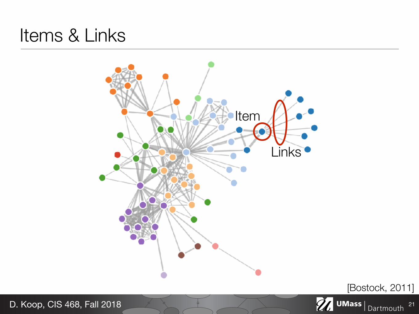
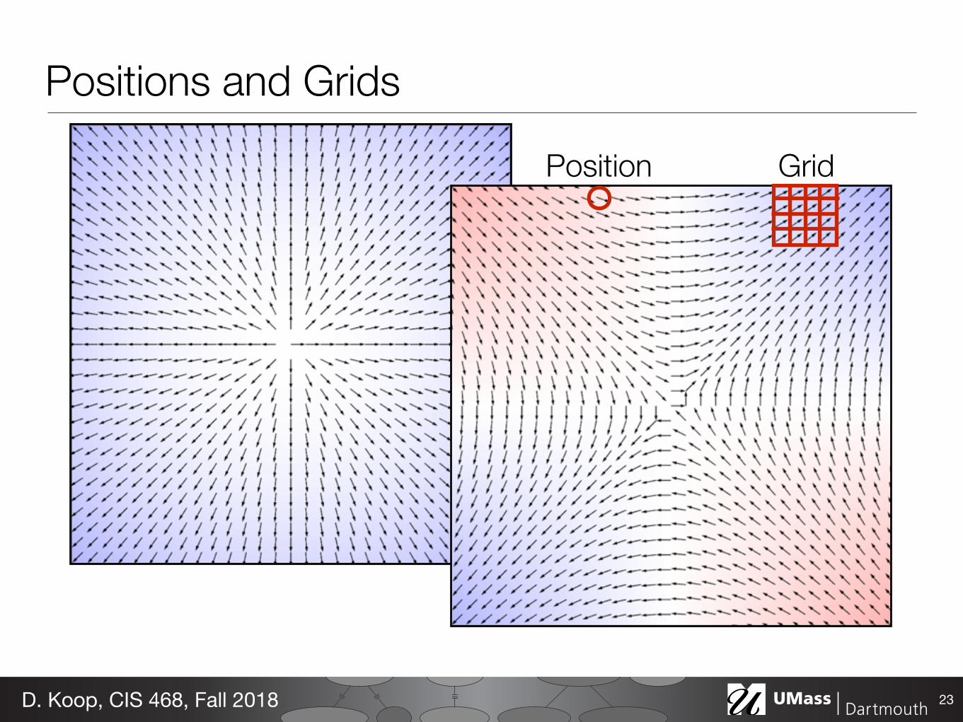
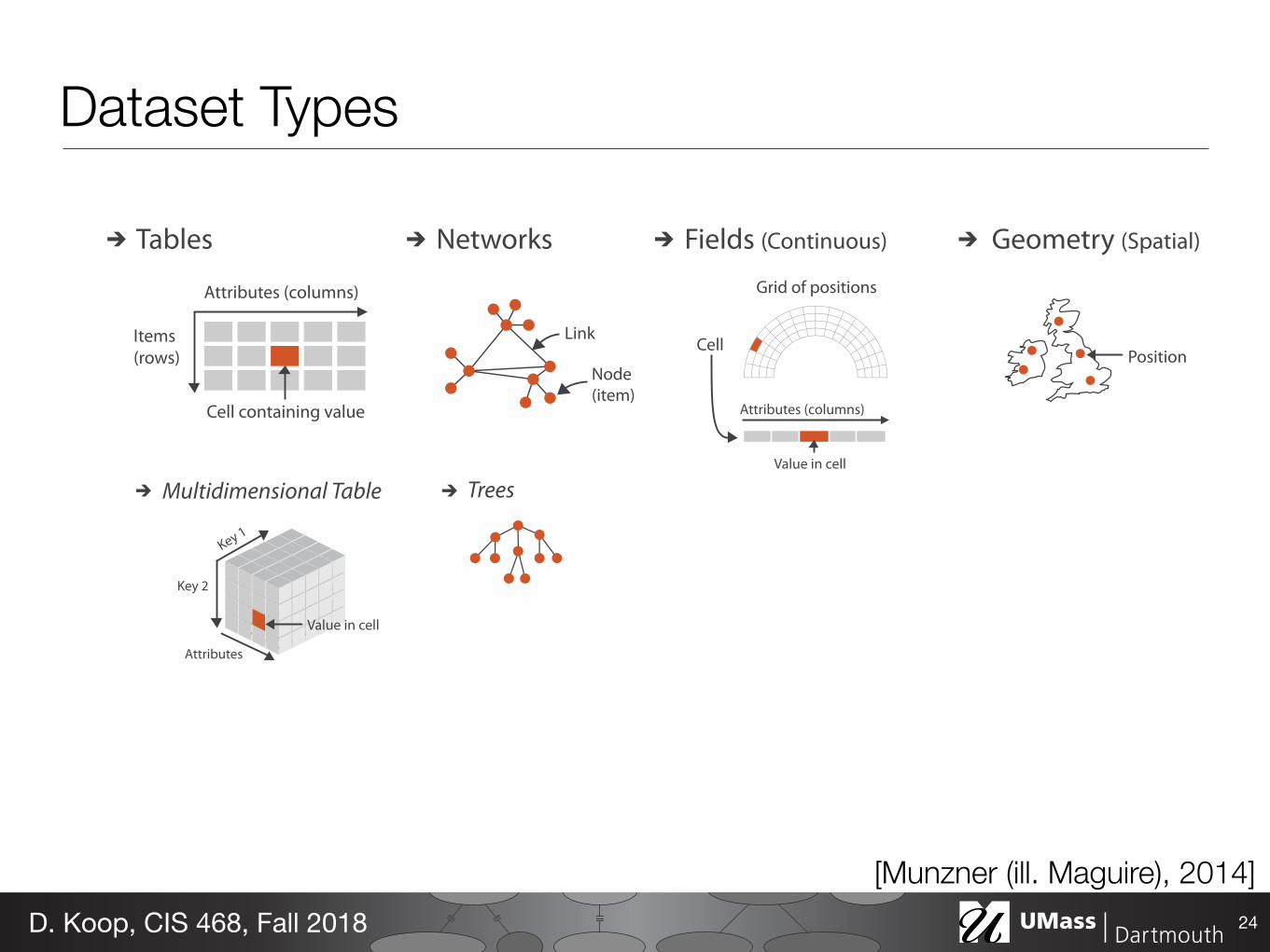
Dataset Types
24
Tables
Attributes (columns)
Items (rows)
Cell containing value
Networks
Link
Node (item)
Trees
Fields (Continuous)
Attributes (columns)
Value in cell
Cell
Multidimensional Table
Value in cell
Grid of positions
Geometry (Spatial)
Position
Dataset Types
[Munzner (ill Maguire) 2014]D Koop CIS 468 Fall 2018
Tables
25
Fieldattribute
itemcell
D Koop CIS 468 Fall 2018
Attribute SemanticsKeys vs Values (Tables) or Independent vs Dependent (Fields)
Flat
Multidimensional
Tabl
es
Fiel
ds
Tablesbull Data organized by rows amp columns
- row ~ item (usually) - column ~ attribute - label ~ attribute name
bull Key identifies each item (row) - Usually unique - Allows join of data from 2+ tables - Compound key key split among
multiple columns eg (state year) for population
bull Multidimensional - Split compound key - eg a data cube with (state year)
26
[Munzner (ill Maguire) 2014]D Koop CIS 468 Fall 2018
Table Visualizations
27
0
0
0
0
0
0
00
5
5
5
5
5
5
55
10
10
10
10
10
10
1010
15
15
15
15
15
15
1515
20
20
20
20
20
20
2020
25
25
25
25
25
25
2525
30
30
30
30
30
30
3030
35
35
35
35
35
35
3535
40
40
40
40
40
40
4040
45
45
45
45
45
45
4545
economy (mpg)
economy (mpg)
economy (mpg)
economy (mpg)
economy (mpg)
economy (mpg)
economy (mpg)economy (mpg)
30
30
30
30
30
30
3030
35
35
35
35
35
35
3535
40
40
40
40
40
40
4040
45
45
45
45
45
45
4545
50
50
50
50
50
50
5050
55
55
55
55
55
55
5555
60
60
60
60
60
60
6060
65
65
65
65
65
65
6565
70
70
70
70
70
70
7070
75
75
75
75
75
75
7575
80
80
80
80
80
80
8080cylinders
cylinders
cylinders
cylinders
cylinders
cylinders
cylinderscylinders
100
100
100
100
100
100
100100
150
150
150
150
150
150
150150
200
200
200
200
200
200
200200
250
250
250
250
250
250
250250
300
300
300
300
300
300
300300
350
350
350
350
350
350
350350
400
400
400
400
400
400
400400
450
450
450
450
450
450
450450
displacement (cc)
displacement (cc)
displacement (cc)
displacement (cc)
displacement (cc)
displacement (cc)
displacement (cc)displacement (cc)
0
0
0
0
0
0
00
20
20
20
20
20
20
2020
40
40
40
40
40
40
4040
60
60
60
60
60
60
6060
80
80
80
80
80
80
8080
100
100
100
100
100
100
100100
120
120
120
120
120
120
120120
140
140
140
140
140
140
140140
160
160
160
160
160
160
160160
180
180
180
180
180
180
180180
200
200
200
200
200
200
200200
220
220
220
220
220
220
220220
power (hp)
power (hp)
power (hp)
power (hp)
power (hp)
power (hp)
power (hp)power (hp)
2000
2000
2000
2000
2000
2000
20002000
2500
2500
2500
2500
2500
2500
25002500
3000
3000
3000
3000
3000
3000
30003000
3500
3500
3500
3500
3500
3500
35003500
4000
4000
4000
4000
4000
4000
40004000
4500
4500
4500
4500
4500
4500
45004500
5000
5000
5000
5000
5000
5000
50005000
weight (lb)
weight (lb)
weight (lb)
weight (lb)
weight (lb)
weight (lb)
weight (lb)weight (lb)
8
8
8
8
8
8
88
10
10
10
10
10
10
1010
12
12
12
12
12
12
1212
14
14
14
14
14
14
1414
16
16
16
16
16
16
1616
18
18
18
18
18
18
1818
20
20
20
20
20
20
2020
22
22
22
22
22
22
2222
24
24
24
24
24
24
2424
0-60 mph (s)
0-60 mph (s)
0-60 mph (s)
0-60 mph (s)
0-60 mph (s)
0-60 mph (s)
0-60 mph (s)0-60 mph (s)
70
70
70
70
70
70
7070
71
71
71
71
71
71
7171
72
72
72
72
72
72
7272
73
73
73
73
73
73
7373
74
74
74
74
74
74
7474
75
75
75
75
75
75
7575
76
76
76
76
76
76
7676
77
77
77
77
77
77
7777
78
78
78
78
78
78
7878
79
79
79
79
79
79
7979
80
80
80
80
80
80
8080
81
81
81
81
81
81
8181
82
82
82
82
82
82
8282year
year
year
year
year
year
yearyear
[M Bostock 2011]D Koop CIS 468 Fall 2018
Networksbull Why networks instead of graphs bull Tables can represent networks
- Many-many relationships - Also can be stored as specific
graph databases or files
28D Koop CIS 468 Fall 2018
Networks
29
Danny Holten amp Jarke J van Wijk Force-Directed Edge Bundling for Graph Visualization
Figure 7 US airlines graph (235 nodes 2101 edges) (a) not bundled and bundled using (b) FDEB with inverse-linear model(c) GBEB and (d) FDEB with inverse-quadratic model
Figure 8 US migration graph (1715 nodes 9780 edges) (a) not bundled and bundled using (b) FDEB with inverse-linearmodel (c) GBEB and (d) FDEB with inverse-quadratic model The same migration flow is highlighted in each graph
Figure 9 A low amount of straightening provides an indication of the number of edges comprising a bundle by widening thebundle (a) s = 0 (b) s = 10 and (c) s = 40 If s is 0 color more clearly indicates the number of edges comprising a bundle
we generated use the rendering technique described in Sec-tion 41 To facilitate the comparison of migration flow inFigure 8 we use a similar rendering technique as the onethat Cui et al [CZQ08] used to generate Figure 8c
The airlines graph is comprised of 235 nodes and 2101edges It took 19 seconds to calculate the bundled airlinesgraphs (Figures 7b and 7d) using the calculation scheme pre-
sented in Section 33 The migration graph is comprised of1715 nodes and 9780 edges It took 80 seconds to calculatethe bundled migration graphs (Figures 8b and 8d) using thesame calculation scheme All measurements were performedon an Intel Core 2 Duo 266GHz PC running Windows XPwith 2GB of RAM and a GeForce 8800GT graphics cardOur prototype was implemented in Borland Delphi 7
c 2009 The Author(s)Journal compilation c 2009 The Eurographics Association and Blackwell Publishing Ltd
[Holten amp van Wijk 2009]D Koop CIS 468 Fall 2018
Networks
30
[Holten amp van Wijk 2009]D Koop CIS 468 Fall 2018
Danny Holten amp Jarke J van Wijk Force-Directed Edge Bundling for Graph Visualization
Figure 7 US airlines graph (235 nodes 2101 edges) (a) not bundled and bundled using (b) FDEB with inverse-linear model(c) GBEB and (d) FDEB with inverse-quadratic model
Figure 8 US migration graph (1715 nodes 9780 edges) (a) not bundled and bundled using (b) FDEB with inverse-linearmodel (c) GBEB and (d) FDEB with inverse-quadratic model The same migration flow is highlighted in each graph
Figure 9 A low amount of straightening provides an indication of the number of edges comprising a bundle by widening thebundle (a) s = 0 (b) s = 10 and (c) s = 40 If s is 0 color more clearly indicates the number of edges comprising a bundle
we generated use the rendering technique described in Sec-tion 41 To facilitate the comparison of migration flow inFigure 8 we use a similar rendering technique as the onethat Cui et al [CZQ08] used to generate Figure 8c
The airlines graph is comprised of 235 nodes and 2101edges It took 19 seconds to calculate the bundled airlinesgraphs (Figures 7b and 7d) using the calculation scheme pre-
sented in Section 33 The migration graph is comprised of1715 nodes and 9780 edges It took 80 seconds to calculatethe bundled migration graphs (Figures 8b and 8d) using thesame calculation scheme All measurements were performedon an Intel Core 2 Duo 266GHz PC running Windows XPwith 2GB of RAM and a GeForce 8800GT graphics cardOur prototype was implemented in Borland Delphi 7
c 2009 The Author(s)Journal compilation c 2009 The Eurographics Association and Blackwell Publishing Ltd
Fields
31D Koop CIS 468 Fall 2018
Scalar Fields Vector Fields Tensor Fields
Each point in space has an associated
Vector Fields
s0
2
400 01 02
10 11 12
20 21 22
3
5
2
4v0
v1
v2
3
5
Fields
31D Koop CIS 468 Fall 2018
Scalar Fields Vector Fields Tensor Fields(Order-1 Tensor Fields)(Order-0 Tensor Fields) (Order-2+)
Each point in space has an associated
Scalar
Vector Fields
Vector Tensor
Fieldsbull Difference between continuous and discrete values bull Examples temperature pressure density bull Grids necessary to sample continuous data
bull Interpolation ldquohow to show values between the sampled points in ways that do not misleadrdquo
32D Koop CIS 468 Fall 2018
Grids (Meshes)bull Meshes combine positional information (geometry) with
topological information (connectivity)
bull Mesh type can differ substantial depending in the way mesh cells are formed
From Weiskopf Machiraju Moumlllercopy WeiskopfMachirajuMoumlller
Data Structures
bull Grid typesndash Grids differ substantially in the cells (basic
building blocks) they are constructed from and in the way the topological information is given
scattered uniform rectilinear structured unstructured[Weiskopf Machiraju Moumlller]
Spatial Data Example MRI
33
[via Levine 2014]D Koop CIS 468 Fall 2018
Scivis and Infovisbull Two subfields of visualization bull Scivis deals with data where the spatial position is given with data
- Usually continuous data - Often displaying physical phenonema - Techniques like isosurfacing volume rendering vector field vis
bull In Infovis the data has no set spatial representation designer chooses how to visually represent data
bull Also compare background colors of visualizations )
34D Koop CIS 468 Fall 2018
SciVis
35
[Google Image Search for scientific visualization 2017]D Koop CIS 468 Fall 2018
InfoVis
36
[Google Image Search for information visualization 2017]D Koop CIS 468 Fall 2018
Sets amp Lists
37
[Daniels httpexperimentsundercurrentcom]D Koop CIS 468 Fall 2018
Attribute Types
38
Attributes
Attribute Types
Ordering Direction
Categorical Ordered
Ordinal Quantitative
Sequential Diverging Cyclic
[Munzner (ill Maguire) 2014]D Koop CIS 468 Fall 2018
Categorial Ordinal and Quantitative
39
231 = Quantitative2 = Nominal3 = Ordinal
quantitative ordinal categorical
D Koop CIS 468 Fall 2018
Categorial Ordinal and Quantitative
40
241 = Quantitative2 = Nominal3 = Ordinal
quantitative ordinal categorical
D Koop CIS 468 Fall 2018
Ordering Direction
41
Attributes
Attribute Types
Ordering Direction
Categorical Ordered
Ordinal Quantitative
Sequential Diverging Cyclic
[Munzner (ill Maguire) 2014]D Koop CIS 468 Fall 2018
Sequential and Diverging Databull Sequential homogenous range
from a minimum to a maximum - Examples Land elevations ocean
depths bull Diverging can be deconstructed
into two sequences pointing in opposite directions - Has a zero point (not necessary 0) - Example Map of both land
elevation and ocean depth
42
[Rogowitz amp Treinish 1998]D Koop CIS 468 Fall 2018
Cyclic Data
43
lar structure of spirals allows for an easy detection of cyclesand for the comparison of periodic data sets Furthermorethe continuity of the data is expressed by using a spiral in-stead of a circle
31 Mathematical description and types of spirals
A spiral is easy to describe and understand in polar coor-dinates ie in the form The distinctive feature ofa spiral is that f is a monotone function In this work we as-sume a spiral is described by
Several simple functions f lead to well-known types ofspirals bull Archimedeslsquo spiral has the form It has the spe-
cial property that a ray emanating from the origincrosses two consecutive arcs of the spiral in a constantdistance
bull The Hyperbolic spiral has the form It is theinverse of Archimedeslsquo spiral with respect to the origin
bull More generally spirals of the form are calledArchimedean spirals
bull The logarithmic spiral has the form It has thespecial property that all arcs cut a ray emanating fromthe origin under the same angleFor the visualization of time-dependent data Archimedeslsquo
spiral seems to be the most appropriate In most applicationsdata from different periods are equally important Thisshould be reflected visually in that the distance to other peri-ods is always the same
32 Mapping data to the spiral
In general markers bars and line elements can be usedto visualize time-series data similar to standard point barand line graphs on Spiral Graphs For instance quantitativediscrete data can be presented as bars on the spiral or bymarks with a corresponding distance to the spiral Howeversince the x and y coordinate are needed to achieve the generalform of the spiral their use is limited for the display of datavalues One might consider to map data values to small ab-solute changes in the radius ie
Yet we have found this way of visualizing to be ineffec-tive We conclude that the general shape of the spiral shouldbe untouched and other attributes should be used such asbull colourbull texture including line styles and patterns
Figure 1Two visualizations of sunshine intensity using about the same screen real estate and thesame color coding scheme In the spiral visualization it is much easier to compare days to spotcloudy time periods or to see events like sunrise and sunset
r f ϕ( )=
r f ϕ( ) dfdϕ------ 0 ϕ R+isingt=
r aϕ=
2πar a ϕfrasl=
r aϕk=
r aekϕ=
r aϕ bv ϕ( ) b πamax v ϕ( )( )---------------------------lt+=
[Sunlight intensity Weber et al 2001]D Koop CIS 468 Fall 2018
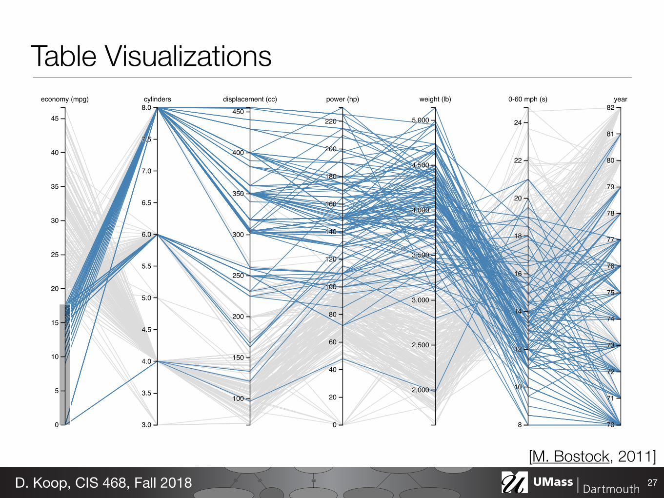
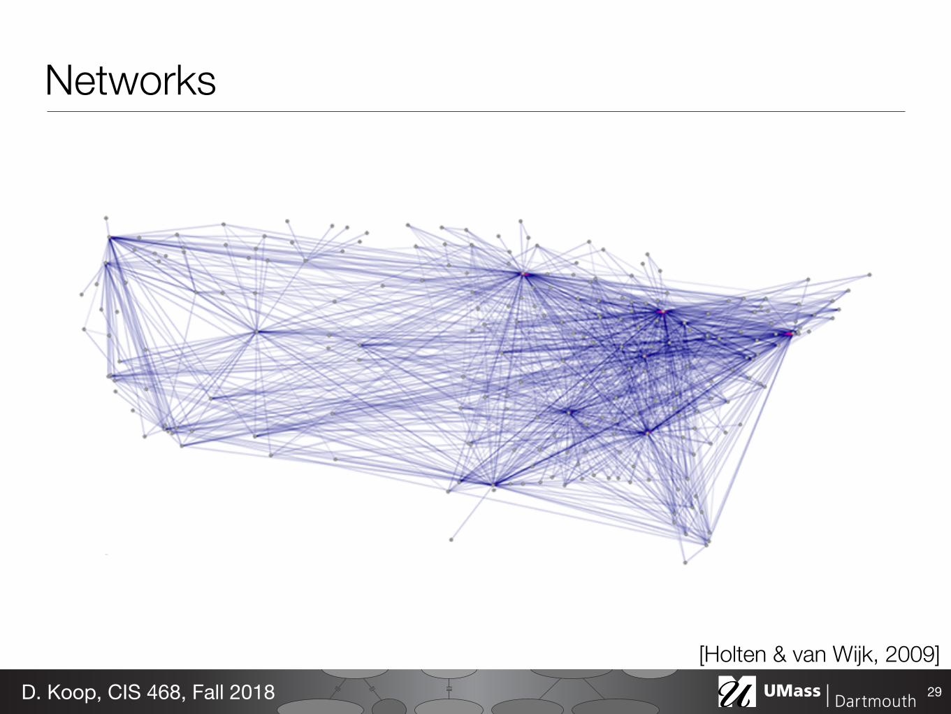
Networks
30
[Holten amp van Wijk 2009]D Koop CIS 468 Fall 2018
Danny Holten amp Jarke J van Wijk Force-Directed Edge Bundling for Graph Visualization
Figure 7 US airlines graph (235 nodes 2101 edges) (a) not bundled and bundled using (b) FDEB with inverse-linear model(c) GBEB and (d) FDEB with inverse-quadratic model
Figure 8 US migration graph (1715 nodes 9780 edges) (a) not bundled and bundled using (b) FDEB with inverse-linearmodel (c) GBEB and (d) FDEB with inverse-quadratic model The same migration flow is highlighted in each graph
Figure 9 A low amount of straightening provides an indication of the number of edges comprising a bundle by widening thebundle (a) s = 0 (b) s = 10 and (c) s = 40 If s is 0 color more clearly indicates the number of edges comprising a bundle
we generated use the rendering technique described in Sec-tion 41 To facilitate the comparison of migration flow inFigure 8 we use a similar rendering technique as the onethat Cui et al [CZQ08] used to generate Figure 8c
The airlines graph is comprised of 235 nodes and 2101edges It took 19 seconds to calculate the bundled airlinesgraphs (Figures 7b and 7d) using the calculation scheme pre-
sented in Section 33 The migration graph is comprised of1715 nodes and 9780 edges It took 80 seconds to calculatethe bundled migration graphs (Figures 8b and 8d) using thesame calculation scheme All measurements were performedon an Intel Core 2 Duo 266GHz PC running Windows XPwith 2GB of RAM and a GeForce 8800GT graphics cardOur prototype was implemented in Borland Delphi 7
c 2009 The Author(s)Journal compilation c 2009 The Eurographics Association and Blackwell Publishing Ltd
Fields
31D Koop CIS 468 Fall 2018
Scalar Fields Vector Fields Tensor Fields
Each point in space has an associated
Vector Fields
s0
2
400 01 02
10 11 12
20 21 22
3
5
2
4v0
v1
v2
3
5
Fields
31D Koop CIS 468 Fall 2018
Scalar Fields Vector Fields Tensor Fields(Order-1 Tensor Fields)(Order-0 Tensor Fields) (Order-2+)
Each point in space has an associated
Scalar
Vector Fields
Vector Tensor
Fieldsbull Difference between continuous and discrete values bull Examples temperature pressure density bull Grids necessary to sample continuous data
bull Interpolation ldquohow to show values between the sampled points in ways that do not misleadrdquo
32D Koop CIS 468 Fall 2018
Grids (Meshes)bull Meshes combine positional information (geometry) with
topological information (connectivity)
bull Mesh type can differ substantial depending in the way mesh cells are formed
From Weiskopf Machiraju Moumlllercopy WeiskopfMachirajuMoumlller
Data Structures
bull Grid typesndash Grids differ substantially in the cells (basic
building blocks) they are constructed from and in the way the topological information is given
scattered uniform rectilinear structured unstructured[Weiskopf Machiraju Moumlller]
Spatial Data Example MRI
33
[via Levine 2014]D Koop CIS 468 Fall 2018
Scivis and Infovisbull Two subfields of visualization bull Scivis deals with data where the spatial position is given with data
- Usually continuous data - Often displaying physical phenonema - Techniques like isosurfacing volume rendering vector field vis
bull In Infovis the data has no set spatial representation designer chooses how to visually represent data
bull Also compare background colors of visualizations )
34D Koop CIS 468 Fall 2018
SciVis
35
[Google Image Search for scientific visualization 2017]D Koop CIS 468 Fall 2018
InfoVis
36
[Google Image Search for information visualization 2017]D Koop CIS 468 Fall 2018
Sets amp Lists
37
[Daniels httpexperimentsundercurrentcom]D Koop CIS 468 Fall 2018
Attribute Types
38
Attributes
Attribute Types
Ordering Direction
Categorical Ordered
Ordinal Quantitative
Sequential Diverging Cyclic
[Munzner (ill Maguire) 2014]D Koop CIS 468 Fall 2018
Categorial Ordinal and Quantitative
39
231 = Quantitative2 = Nominal3 = Ordinal
quantitative ordinal categorical
D Koop CIS 468 Fall 2018
Categorial Ordinal and Quantitative
40
241 = Quantitative2 = Nominal3 = Ordinal
quantitative ordinal categorical
D Koop CIS 468 Fall 2018
Ordering Direction
41
Attributes
Attribute Types
Ordering Direction
Categorical Ordered
Ordinal Quantitative
Sequential Diverging Cyclic
[Munzner (ill Maguire) 2014]D Koop CIS 468 Fall 2018
Sequential and Diverging Databull Sequential homogenous range
from a minimum to a maximum - Examples Land elevations ocean
depths bull Diverging can be deconstructed
into two sequences pointing in opposite directions - Has a zero point (not necessary 0) - Example Map of both land
elevation and ocean depth
42
[Rogowitz amp Treinish 1998]D Koop CIS 468 Fall 2018
Cyclic Data
43
lar structure of spirals allows for an easy detection of cyclesand for the comparison of periodic data sets Furthermorethe continuity of the data is expressed by using a spiral in-stead of a circle
31 Mathematical description and types of spirals
A spiral is easy to describe and understand in polar coor-dinates ie in the form The distinctive feature ofa spiral is that f is a monotone function In this work we as-sume a spiral is described by
Several simple functions f lead to well-known types ofspirals bull Archimedeslsquo spiral has the form It has the spe-
cial property that a ray emanating from the origincrosses two consecutive arcs of the spiral in a constantdistance
bull The Hyperbolic spiral has the form It is theinverse of Archimedeslsquo spiral with respect to the origin
bull More generally spirals of the form are calledArchimedean spirals
bull The logarithmic spiral has the form It has thespecial property that all arcs cut a ray emanating fromthe origin under the same angleFor the visualization of time-dependent data Archimedeslsquo
spiral seems to be the most appropriate In most applicationsdata from different periods are equally important Thisshould be reflected visually in that the distance to other peri-ods is always the same
32 Mapping data to the spiral
In general markers bars and line elements can be usedto visualize time-series data similar to standard point barand line graphs on Spiral Graphs For instance quantitativediscrete data can be presented as bars on the spiral or bymarks with a corresponding distance to the spiral Howeversince the x and y coordinate are needed to achieve the generalform of the spiral their use is limited for the display of datavalues One might consider to map data values to small ab-solute changes in the radius ie
Yet we have found this way of visualizing to be ineffec-tive We conclude that the general shape of the spiral shouldbe untouched and other attributes should be used such asbull colourbull texture including line styles and patterns
Figure 1Two visualizations of sunshine intensity using about the same screen real estate and thesame color coding scheme In the spiral visualization it is much easier to compare days to spotcloudy time periods or to see events like sunrise and sunset
r f ϕ( )=
r f ϕ( ) dfdϕ------ 0 ϕ R+isingt=
r aϕ=
2πar a ϕfrasl=
r aϕk=
r aekϕ=
r aϕ bv ϕ( ) b πamax v ϕ( )( )---------------------------lt+=
[Sunlight intensity Weber et al 2001]D Koop CIS 468 Fall 2018
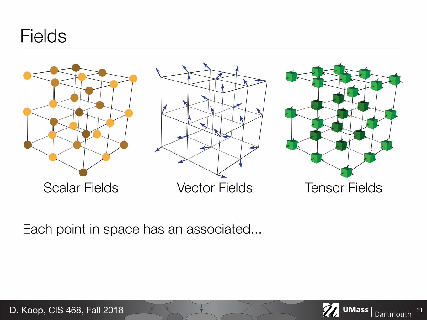
Fields
31D Koop CIS 468 Fall 2018
Scalar Fields Vector Fields Tensor Fields
Each point in space has an associated
Vector Fields
s0
2
400 01 02
10 11 12
20 21 22
3
5
2
4v0
v1
v2
3
5
Fields
31D Koop CIS 468 Fall 2018
Scalar Fields Vector Fields Tensor Fields(Order-1 Tensor Fields)(Order-0 Tensor Fields) (Order-2+)
Each point in space has an associated
Scalar
Vector Fields
Vector Tensor
Fieldsbull Difference between continuous and discrete values bull Examples temperature pressure density bull Grids necessary to sample continuous data
bull Interpolation ldquohow to show values between the sampled points in ways that do not misleadrdquo
32D Koop CIS 468 Fall 2018
Grids (Meshes)bull Meshes combine positional information (geometry) with
topological information (connectivity)
bull Mesh type can differ substantial depending in the way mesh cells are formed
From Weiskopf Machiraju Moumlllercopy WeiskopfMachirajuMoumlller
Data Structures
bull Grid typesndash Grids differ substantially in the cells (basic
building blocks) they are constructed from and in the way the topological information is given
scattered uniform rectilinear structured unstructured[Weiskopf Machiraju Moumlller]
Spatial Data Example MRI
33
[via Levine 2014]D Koop CIS 468 Fall 2018
Scivis and Infovisbull Two subfields of visualization bull Scivis deals with data where the spatial position is given with data
- Usually continuous data - Often displaying physical phenonema - Techniques like isosurfacing volume rendering vector field vis
bull In Infovis the data has no set spatial representation designer chooses how to visually represent data
bull Also compare background colors of visualizations )
34D Koop CIS 468 Fall 2018
SciVis
35
[Google Image Search for scientific visualization 2017]D Koop CIS 468 Fall 2018
InfoVis
36
[Google Image Search for information visualization 2017]D Koop CIS 468 Fall 2018
Sets amp Lists
37
[Daniels httpexperimentsundercurrentcom]D Koop CIS 468 Fall 2018
Attribute Types
38
Attributes
Attribute Types
Ordering Direction
Categorical Ordered
Ordinal Quantitative
Sequential Diverging Cyclic
[Munzner (ill Maguire) 2014]D Koop CIS 468 Fall 2018
Categorial Ordinal and Quantitative
39
231 = Quantitative2 = Nominal3 = Ordinal
quantitative ordinal categorical
D Koop CIS 468 Fall 2018
Categorial Ordinal and Quantitative
40
241 = Quantitative2 = Nominal3 = Ordinal
quantitative ordinal categorical
D Koop CIS 468 Fall 2018
Ordering Direction
41
Attributes
Attribute Types
Ordering Direction
Categorical Ordered
Ordinal Quantitative
Sequential Diverging Cyclic
[Munzner (ill Maguire) 2014]D Koop CIS 468 Fall 2018
Sequential and Diverging Databull Sequential homogenous range
from a minimum to a maximum - Examples Land elevations ocean
depths bull Diverging can be deconstructed
into two sequences pointing in opposite directions - Has a zero point (not necessary 0) - Example Map of both land
elevation and ocean depth
42
[Rogowitz amp Treinish 1998]D Koop CIS 468 Fall 2018
Cyclic Data
43
lar structure of spirals allows for an easy detection of cyclesand for the comparison of periodic data sets Furthermorethe continuity of the data is expressed by using a spiral in-stead of a circle
31 Mathematical description and types of spirals
A spiral is easy to describe and understand in polar coor-dinates ie in the form The distinctive feature ofa spiral is that f is a monotone function In this work we as-sume a spiral is described by
Several simple functions f lead to well-known types ofspirals bull Archimedeslsquo spiral has the form It has the spe-
cial property that a ray emanating from the origincrosses two consecutive arcs of the spiral in a constantdistance
bull The Hyperbolic spiral has the form It is theinverse of Archimedeslsquo spiral with respect to the origin
bull More generally spirals of the form are calledArchimedean spirals
bull The logarithmic spiral has the form It has thespecial property that all arcs cut a ray emanating fromthe origin under the same angleFor the visualization of time-dependent data Archimedeslsquo
spiral seems to be the most appropriate In most applicationsdata from different periods are equally important Thisshould be reflected visually in that the distance to other peri-ods is always the same
32 Mapping data to the spiral
In general markers bars and line elements can be usedto visualize time-series data similar to standard point barand line graphs on Spiral Graphs For instance quantitativediscrete data can be presented as bars on the spiral or bymarks with a corresponding distance to the spiral Howeversince the x and y coordinate are needed to achieve the generalform of the spiral their use is limited for the display of datavalues One might consider to map data values to small ab-solute changes in the radius ie
Yet we have found this way of visualizing to be ineffec-tive We conclude that the general shape of the spiral shouldbe untouched and other attributes should be used such asbull colourbull texture including line styles and patterns
Figure 1Two visualizations of sunshine intensity using about the same screen real estate and thesame color coding scheme In the spiral visualization it is much easier to compare days to spotcloudy time periods or to see events like sunrise and sunset
r f ϕ( )=
r f ϕ( ) dfdϕ------ 0 ϕ R+isingt=
r aϕ=
2πar a ϕfrasl=
r aϕk=
r aekϕ=
r aϕ bv ϕ( ) b πamax v ϕ( )( )---------------------------lt+=
[Sunlight intensity Weber et al 2001]D Koop CIS 468 Fall 2018
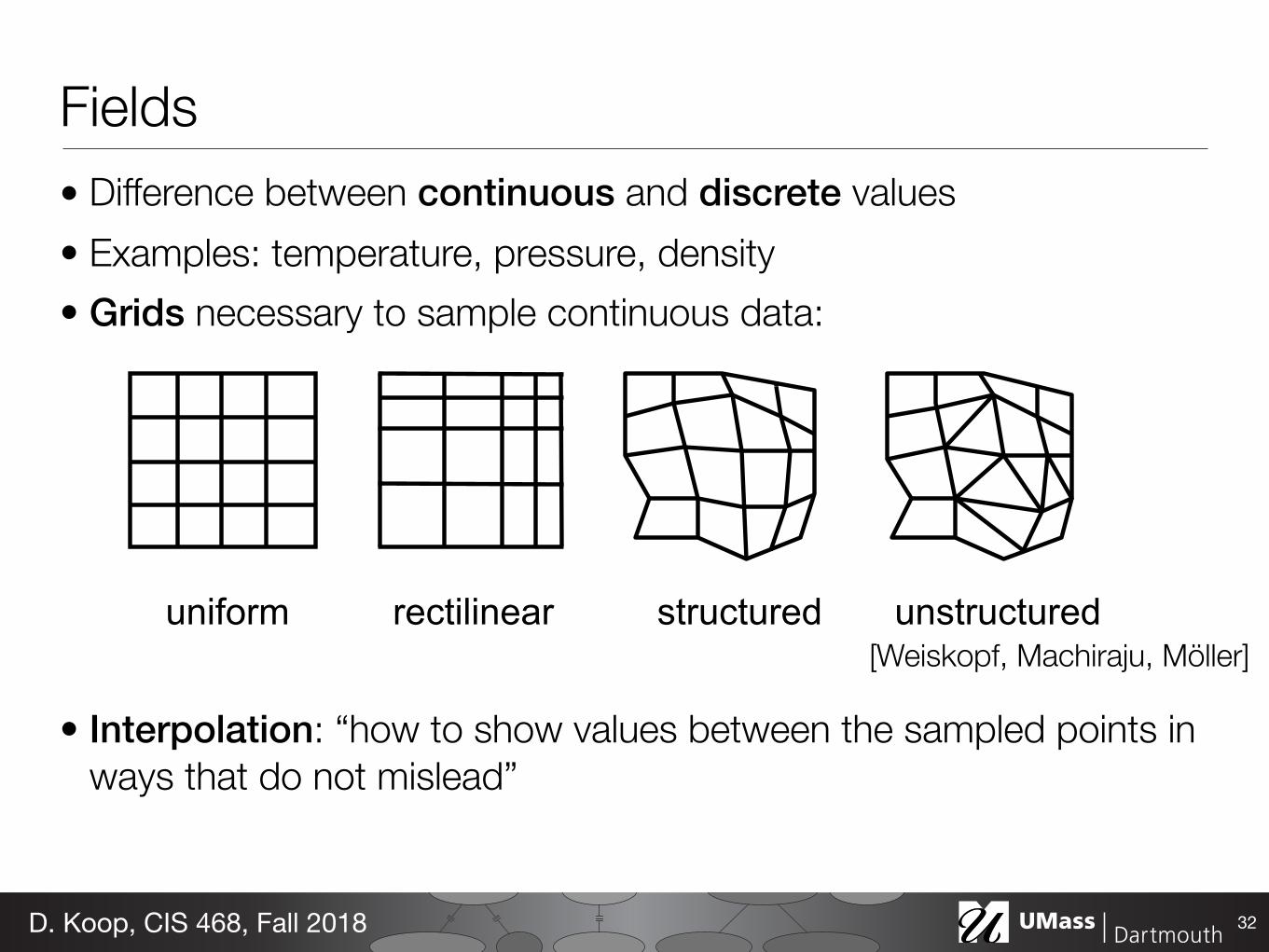
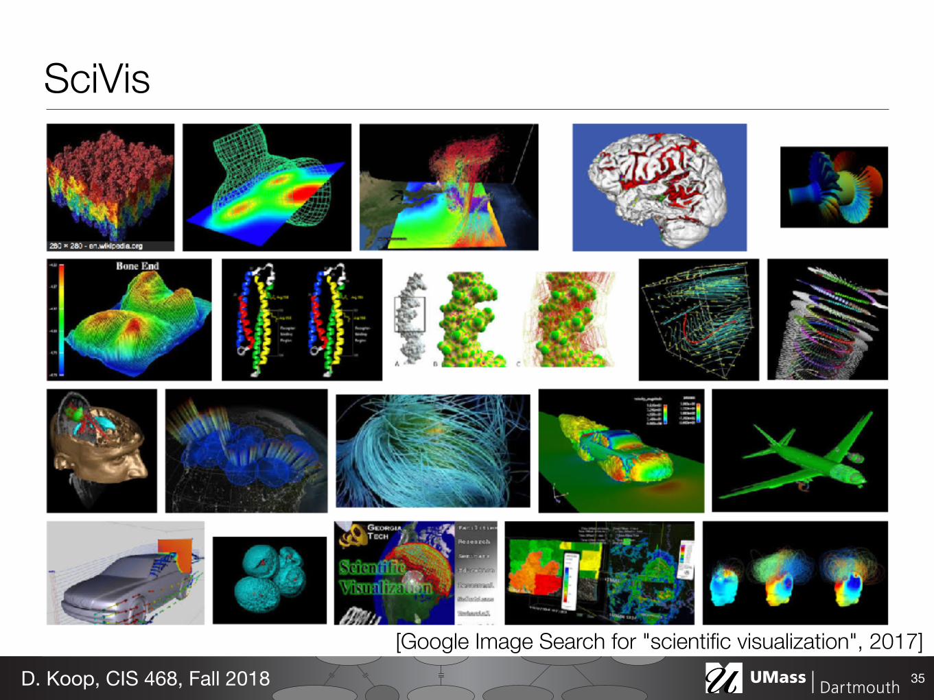
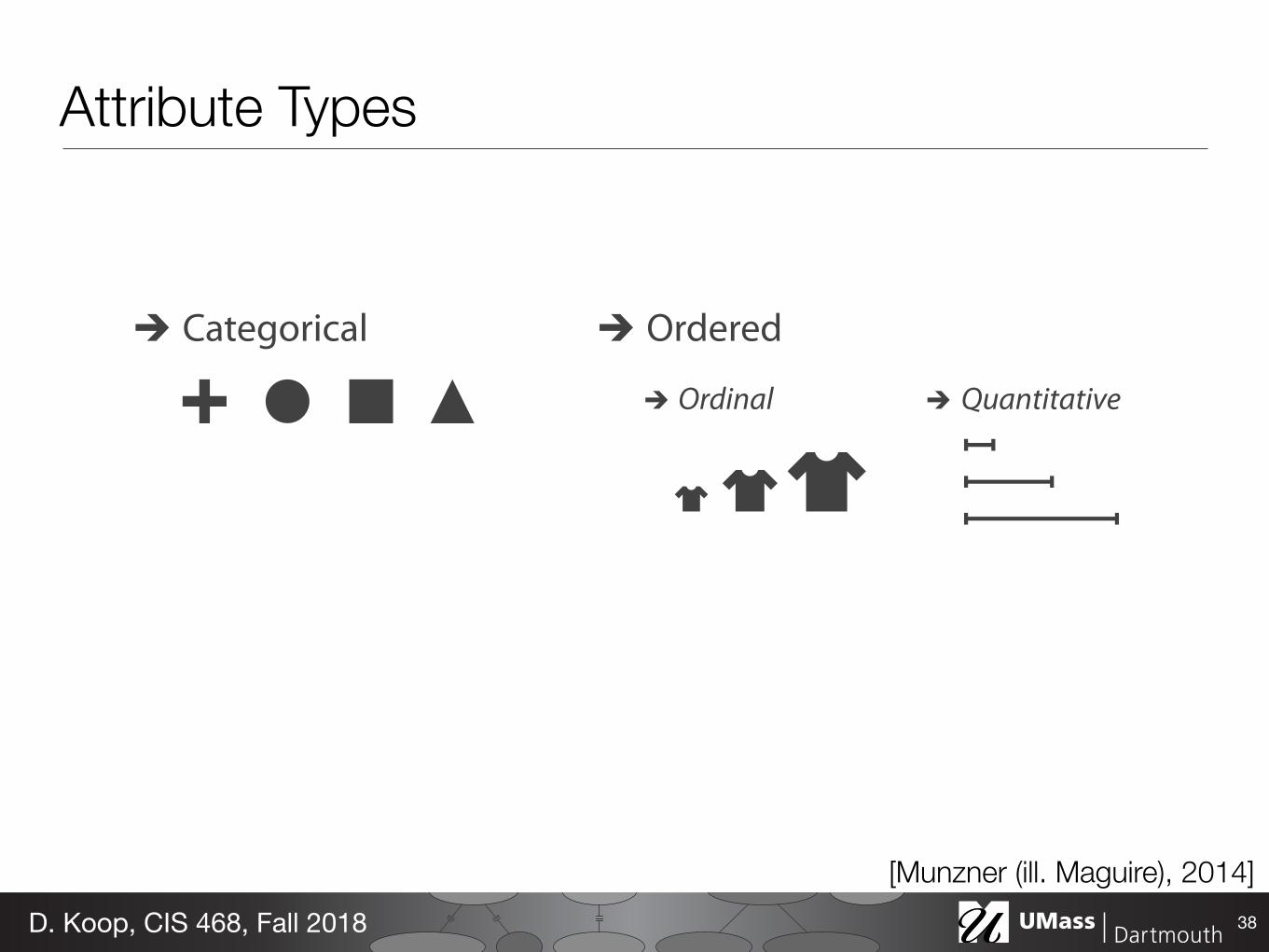
Attribute Types
38
Attributes
Attribute Types
Ordering Direction
Categorical Ordered
Ordinal Quantitative
Sequential Diverging Cyclic
[Munzner (ill Maguire) 2014]D Koop CIS 468 Fall 2018
Categorial Ordinal and Quantitative
39
231 = Quantitative2 = Nominal3 = Ordinal
quantitative ordinal categorical
D Koop CIS 468 Fall 2018
Categorial Ordinal and Quantitative
40
241 = Quantitative2 = Nominal3 = Ordinal
quantitative ordinal categorical
D Koop CIS 468 Fall 2018
Ordering Direction
41
Attributes
Attribute Types
Ordering Direction
Categorical Ordered
Ordinal Quantitative
Sequential Diverging Cyclic
[Munzner (ill Maguire) 2014]D Koop CIS 468 Fall 2018
Sequential and Diverging Databull Sequential homogenous range
from a minimum to a maximum - Examples Land elevations ocean
depths bull Diverging can be deconstructed
into two sequences pointing in opposite directions - Has a zero point (not necessary 0) - Example Map of both land
elevation and ocean depth
42
[Rogowitz amp Treinish 1998]D Koop CIS 468 Fall 2018
Cyclic Data
43
lar structure of spirals allows for an easy detection of cyclesand for the comparison of periodic data sets Furthermorethe continuity of the data is expressed by using a spiral in-stead of a circle
31 Mathematical description and types of spirals
A spiral is easy to describe and understand in polar coor-dinates ie in the form The distinctive feature ofa spiral is that f is a monotone function In this work we as-sume a spiral is described by
Several simple functions f lead to well-known types ofspirals bull Archimedeslsquo spiral has the form It has the spe-
cial property that a ray emanating from the origincrosses two consecutive arcs of the spiral in a constantdistance
bull The Hyperbolic spiral has the form It is theinverse of Archimedeslsquo spiral with respect to the origin
bull More generally spirals of the form are calledArchimedean spirals
bull The logarithmic spiral has the form It has thespecial property that all arcs cut a ray emanating fromthe origin under the same angleFor the visualization of time-dependent data Archimedeslsquo
spiral seems to be the most appropriate In most applicationsdata from different periods are equally important Thisshould be reflected visually in that the distance to other peri-ods is always the same
32 Mapping data to the spiral
In general markers bars and line elements can be usedto visualize time-series data similar to standard point barand line graphs on Spiral Graphs For instance quantitativediscrete data can be presented as bars on the spiral or bymarks with a corresponding distance to the spiral Howeversince the x and y coordinate are needed to achieve the generalform of the spiral their use is limited for the display of datavalues One might consider to map data values to small ab-solute changes in the radius ie
Yet we have found this way of visualizing to be ineffec-tive We conclude that the general shape of the spiral shouldbe untouched and other attributes should be used such asbull colourbull texture including line styles and patterns
Figure 1Two visualizations of sunshine intensity using about the same screen real estate and thesame color coding scheme In the spiral visualization it is much easier to compare days to spotcloudy time periods or to see events like sunrise and sunset
r f ϕ( )=
r f ϕ( ) dfdϕ------ 0 ϕ R+isingt=
r aϕ=
2πar a ϕfrasl=
r aϕk=
r aekϕ=
r aϕ bv ϕ( ) b πamax v ϕ( )( )---------------------------lt+=
[Sunlight intensity Weber et al 2001]D Koop CIS 468 Fall 2018

Categorial Ordinal and Quantitative
40
241 = Quantitative2 = Nominal3 = Ordinal
quantitative ordinal categorical
D Koop CIS 468 Fall 2018
Ordering Direction
41
Attributes
Attribute Types
Ordering Direction
Categorical Ordered
Ordinal Quantitative
Sequential Diverging Cyclic
[Munzner (ill Maguire) 2014]D Koop CIS 468 Fall 2018
Sequential and Diverging Databull Sequential homogenous range
from a minimum to a maximum - Examples Land elevations ocean
depths bull Diverging can be deconstructed
into two sequences pointing in opposite directions - Has a zero point (not necessary 0) - Example Map of both land
elevation and ocean depth
42
[Rogowitz amp Treinish 1998]D Koop CIS 468 Fall 2018
Cyclic Data
43
lar structure of spirals allows for an easy detection of cyclesand for the comparison of periodic data sets Furthermorethe continuity of the data is expressed by using a spiral in-stead of a circle
31 Mathematical description and types of spirals
A spiral is easy to describe and understand in polar coor-dinates ie in the form The distinctive feature ofa spiral is that f is a monotone function In this work we as-sume a spiral is described by
Several simple functions f lead to well-known types ofspirals bull Archimedeslsquo spiral has the form It has the spe-
cial property that a ray emanating from the origincrosses two consecutive arcs of the spiral in a constantdistance
bull The Hyperbolic spiral has the form It is theinverse of Archimedeslsquo spiral with respect to the origin
bull More generally spirals of the form are calledArchimedean spirals
bull The logarithmic spiral has the form It has thespecial property that all arcs cut a ray emanating fromthe origin under the same angleFor the visualization of time-dependent data Archimedeslsquo
spiral seems to be the most appropriate In most applicationsdata from different periods are equally important Thisshould be reflected visually in that the distance to other peri-ods is always the same
32 Mapping data to the spiral
In general markers bars and line elements can be usedto visualize time-series data similar to standard point barand line graphs on Spiral Graphs For instance quantitativediscrete data can be presented as bars on the spiral or bymarks with a corresponding distance to the spiral Howeversince the x and y coordinate are needed to achieve the generalform of the spiral their use is limited for the display of datavalues One might consider to map data values to small ab-solute changes in the radius ie
Yet we have found this way of visualizing to be ineffec-tive We conclude that the general shape of the spiral shouldbe untouched and other attributes should be used such asbull colourbull texture including line styles and patterns
Figure 1Two visualizations of sunshine intensity using about the same screen real estate and thesame color coding scheme In the spiral visualization it is much easier to compare days to spotcloudy time periods or to see events like sunrise and sunset
r f ϕ( )=
r f ϕ( ) dfdϕ------ 0 ϕ R+isingt=
r aϕ=
2πar a ϕfrasl=
r aϕk=
r aekϕ=
r aϕ bv ϕ( ) b πamax v ϕ( )( )---------------------------lt+=
[Sunlight intensity Weber et al 2001]D Koop CIS 468 Fall 2018

Ordering Direction
41
Attributes
Attribute Types
Ordering Direction
Categorical Ordered
Ordinal Quantitative
Sequential Diverging Cyclic
[Munzner (ill Maguire) 2014]D Koop CIS 468 Fall 2018
Sequential and Diverging Databull Sequential homogenous range
from a minimum to a maximum - Examples Land elevations ocean
depths bull Diverging can be deconstructed
into two sequences pointing in opposite directions - Has a zero point (not necessary 0) - Example Map of both land
elevation and ocean depth
42
[Rogowitz amp Treinish 1998]D Koop CIS 468 Fall 2018
Cyclic Data
43
lar structure of spirals allows for an easy detection of cyclesand for the comparison of periodic data sets Furthermorethe continuity of the data is expressed by using a spiral in-stead of a circle
31 Mathematical description and types of spirals
A spiral is easy to describe and understand in polar coor-dinates ie in the form The distinctive feature ofa spiral is that f is a monotone function In this work we as-sume a spiral is described by
Several simple functions f lead to well-known types ofspirals bull Archimedeslsquo spiral has the form It has the spe-
cial property that a ray emanating from the origincrosses two consecutive arcs of the spiral in a constantdistance
bull The Hyperbolic spiral has the form It is theinverse of Archimedeslsquo spiral with respect to the origin
bull More generally spirals of the form are calledArchimedean spirals
bull The logarithmic spiral has the form It has thespecial property that all arcs cut a ray emanating fromthe origin under the same angleFor the visualization of time-dependent data Archimedeslsquo
spiral seems to be the most appropriate In most applicationsdata from different periods are equally important Thisshould be reflected visually in that the distance to other peri-ods is always the same
32 Mapping data to the spiral
In general markers bars and line elements can be usedto visualize time-series data similar to standard point barand line graphs on Spiral Graphs For instance quantitativediscrete data can be presented as bars on the spiral or bymarks with a corresponding distance to the spiral Howeversince the x and y coordinate are needed to achieve the generalform of the spiral their use is limited for the display of datavalues One might consider to map data values to small ab-solute changes in the radius ie
Yet we have found this way of visualizing to be ineffec-tive We conclude that the general shape of the spiral shouldbe untouched and other attributes should be used such asbull colourbull texture including line styles and patterns
Figure 1Two visualizations of sunshine intensity using about the same screen real estate and thesame color coding scheme In the spiral visualization it is much easier to compare days to spotcloudy time periods or to see events like sunrise and sunset
r f ϕ( )=
r f ϕ( ) dfdϕ------ 0 ϕ R+isingt=
r aϕ=
2πar a ϕfrasl=
r aϕk=
r aekϕ=
r aϕ bv ϕ( ) b πamax v ϕ( )( )---------------------------lt+=
[Sunlight intensity Weber et al 2001]D Koop CIS 468 Fall 2018
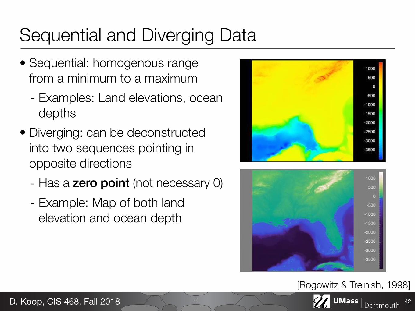


![Data Visualization (CIS 468)dkoop/cis468-2018fa/lectures/lecture17.pdf · representations that may significantly advance the state of the art. REFERENCES [1] C. Ahlberg and B. Shneiderman](https://img.pdfslide.us/doc/110x75/5f6113dd74fa097c854f5656/data-visualization-cis-468-dkoopcis468-2018falectureslecture17pdf-representations.jpg)