Data Validation Overview

Hilary R. HafnerSonoma Technology, Inc.

Petaluma, CA

Presented at2009 National Ambient Air Monitoring Conference

Breakout Session: Data ValidationNashville, TN

November 2-5, 2009

STI-3726

2

Outline

•

Importance of Data Validation•

Data Validation Levels

•

General Approach to Data Validation•

Examples

•

Resources

Data validation is defined as the process of determining the quality of observations

and identifying their validity

3

Why Should You Validate Your Data?

•

It is the monitoring agency’s responsibility to prevent, identify, correct, and define the consequences of monitoring difficulties that might affect the precision and accuracy, and/or the validity, of the measurements.

•

Serious errors in data analysis and modeling (and subsequent policy development) can result from erroneous data values.

•

Accurate information helps you respond to community concerns.

4

Objectives and Benefit

•

The objectives

of the data validation process are to–

produce a database with values that are of a known quality

–

evaluate the internal, spatial, temporal, and physical consistency of the data

–

identify errors, biases, and outliers•

The benefit

for the data analyst who performs

data validation is enhanced familiarity with the unique features of the data set.

5

Data Validation Levels Types of Checks

•

Level I–

Routine checks during the initial data processing and generation of data, including proper data file identification; review of unusual events, field data sheets, and result reports; and instrument performance checks

•

Level II–

Internal consistency tests to identify values in the data that appear atypical when compared to values from the entire data set

–

Comparisons of current data with historical data to verify consistency over time

–

Parallel consistency tests with data sets from the same population (e.g., region, period of time, air mass) to identify systematic bias

6

Level 1: Field and Laboratory Checks

•

Verify computer file entries against data sheets.•

Flag samples when significant deviations from measurement assumptions have occurred.

•

Eliminate values for measurements that are known to be invalid because of instrument malfunctions.

•

Replace data from a backup data acquisition system in the event of primary system failure.

•

Adjust measurement values for quantifiable calibration or interference bias.

7

Level II: Internal Consistency Checks•

Inspect time series to see if concentrations vary by time of day, day of week, and season as expected.

•

Compare pollutant concentrations for expected relationships.

•

Identify and flag unusual values including–

Values that normally follow a qualitatively predictable spatial or temporal pattern

–

Values that normally track the values of other variables in a time series

–

Extreme values, outliers

“The first assumption upon finding a measurement that is inconsistent with physical expectations is that the unusual value is due to a measurement error.

If, upon tracing the path of the measurement, nothing unusual is

found, the value can be assumed to be a valid result of an environmental cause.”

Judy Chow, Desert Research Institute

8

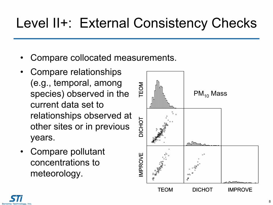
Level II+: External Consistency Checks

•

Compare collocated measurements.•

Compare relationships (e.g., temporal, among species) observed in the current data set to relationships observed at other sites or in previous years.

•

Compare pollutant concentrations to meteorology. IM

PR

OV

ED

ICH

OT

TEO

M

TEOM DICHOT IMPROVE

IMP

RO

VE

DIC

HO

TTE

OM

TEOM DICHOT IMPROVE

PM10

Mass

9

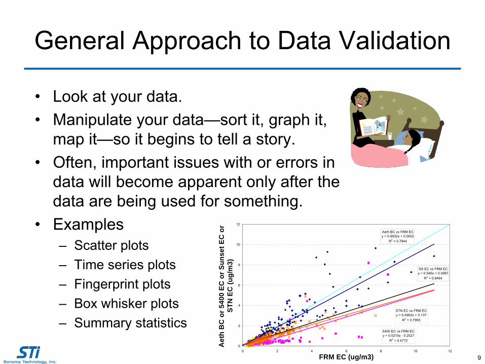
General Approach to Data Validation

•

Look at your data.•

Manipulate your data—sort it, graph it,

map it—so it begins to tell a story.•

Often, important issues with or errors in data will become apparent only after the data are being used for something.

•

Examples–

Scatter plots–

Time series plots–

Fingerprint plots–

Box whisker plots–

Summary statistics

Aeth BC vs FRM ECy = 0.9002x + 0.0652

R2 = 0.7944

5400 EC vs FRM ECy = 0.5215x - 0.2527

R2 = 0.4772

SS EC vs FRM ECy = 0.546x + 0.0987

R2 = 0.8464

STN EC vs FRM ECy = 0.4902x + 0.137

R2 = 0.7993

0

2

4

6

8

10

12

0 2 4 6 8 10 12

FRM EC (ug/m3)

Aet

h B

C o

r 540

0 EC

or S

unse

t EC

or

STN

EC

(ug/

m3)

10

Considerations in Evaluating Your Data

•

Levels of other pollutants•

Time of day/year

•

Observations at other sites•

Audits and inter-laboratory comparisons

•

Instrument performance history•

Calibration drift

•

Site characteristics•

Meteorology

•

Exceptional events

11

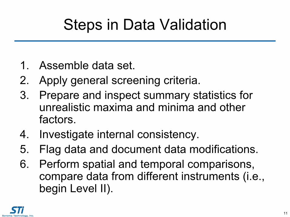
Steps in Data Validation

1.

Assemble data set.2.

Apply general screening criteria.

3.

Prepare and inspect summary statistics for unrealistic maxima and minima and other factors.

4.

Investigate internal consistency.5.

Flag data and document data modifications.

6.

Perform spatial and temporal comparisons, compare data from different instruments (i.e., begin Level II).

12

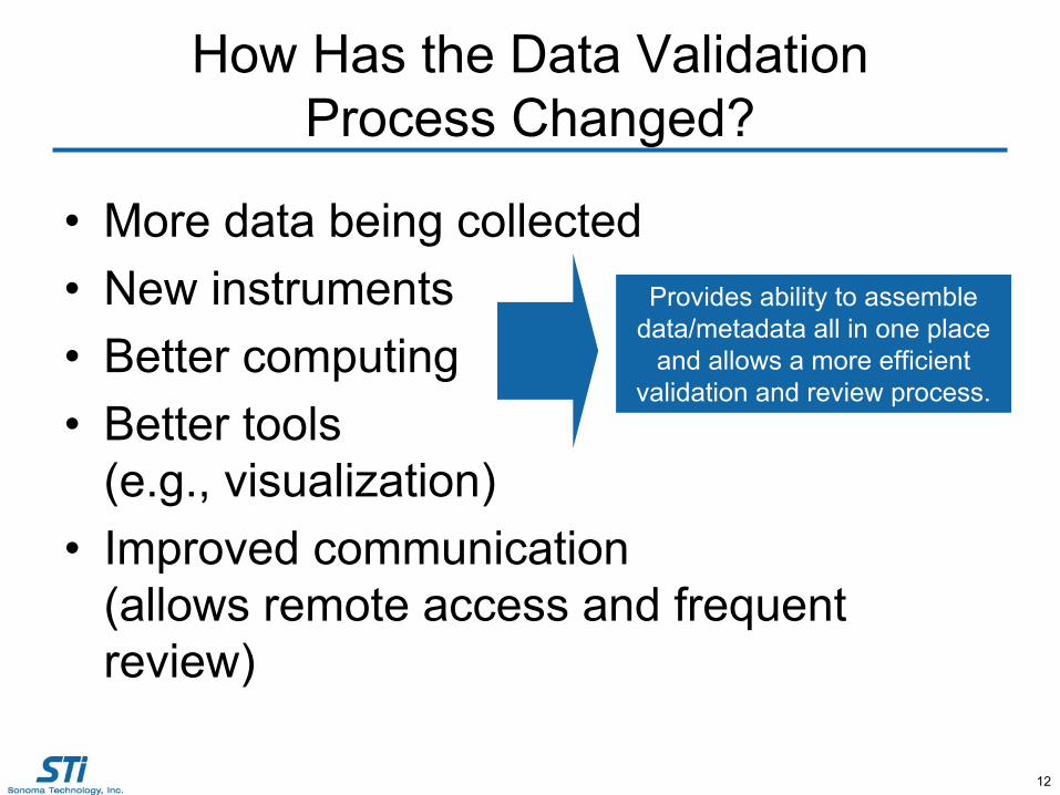
How Has the Data Validation Process Changed?

•

More data being collected•

New instruments

•

Better computing•

Better tools (e.g., visualization)

•

Improved communication (allows remote access and frequent

review)

Provides ability to assemble data/metadata all in one place

and allows a more efficient validation and review process.

13

Automated Quality Assurance Checks

RawData

AmbientAir Quality

DataSelf checks

Instrumentchecks

Site checksNetwork (off-site)

checks

AIRNow

BAAQMDWeb Server Source: Mark Stoelting

14

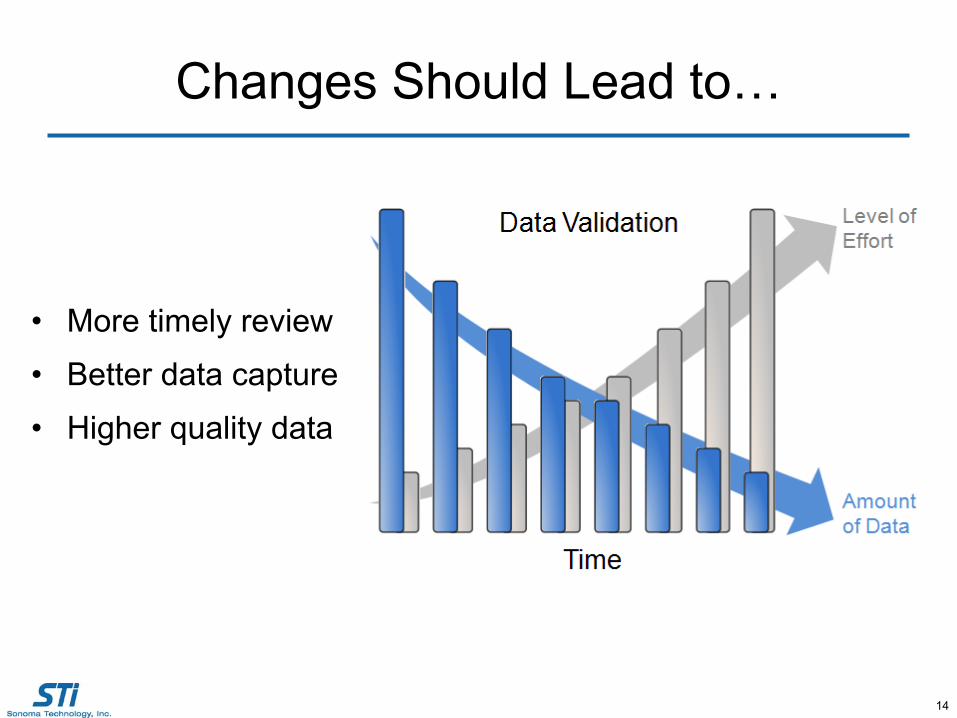
Changes Should Lead to…

•

More timely review

•

Better data capture

•

Higher quality data

15

Importance of Supplemental Data Examples

•

Sample collection specifications –

sampler type, sampling media, inlet type, etc.

•

Sampling location description –

nearby sources, topography, distance to roadways, etc.

•

Audit, blank collection, and collocated sampler descriptions (accuracy and precision)

•

Sample analysis and instrument calibration descriptions

•

Replication and duplication of sample results•

Sample schedule

16

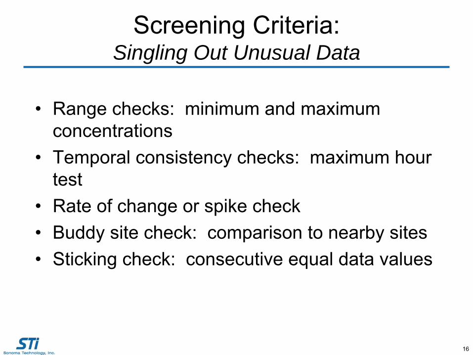
Screening Criteria: Singling Out Unusual Data

•

Range checks: minimum and maximum concentrations

•

Temporal consistency checks: maximum hour test

•

Rate of change or spike check•

Buddy site check: comparison to nearby sites

•

Sticking check: consecutive equal data values

17

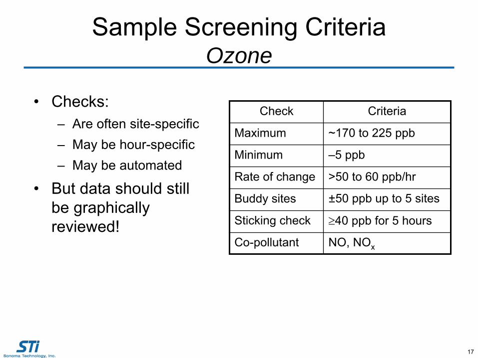
Sample Screening Criteria Ozone

•

Checks:–

Are often site-specific–

May be hour-specific–

May be automated

•

But data should still be graphically reviewed!

Check Criteria

Maximum ~170 to 225 ppb

Minimum –5 ppb

Rate of change >50 to 60 ppb/hr

Buddy sites ±50 ppb up to 5 sites

Sticking check 40 ppb for 5 hours

Co-pollutant NO, NOx

18

AIRNow-Tech

Example –

Ozone Screening

Max Suspect: Still used in spatial mapping

Max Severe: Not used in maps

Note hour-specificscreening

19

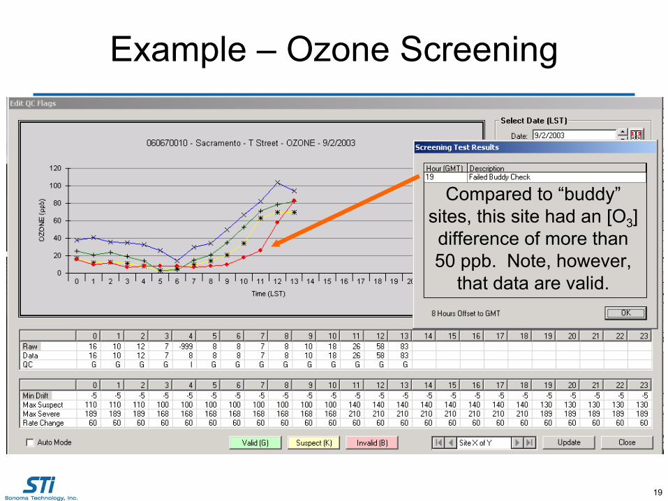
Example –

Ozone Screening

Compared to “buddy”

sites, this site had an [O3

] difference of more than 50 ppb. Note, however,

that data are valid.

21

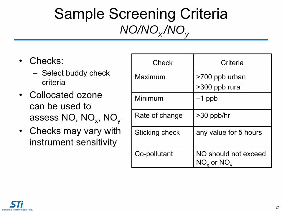
Sample Screening Criteria NO/NOx

•

Checks:–

Select buddy check criteria

•

Collocated ozone can be used to assess NO, NOx

, NOy

•

Checks may vary with instrument sensitivity

Check Criteria

Maximum >700 ppb urban>300 ppb rural

Minimum –1 ppb

Rate of change >30 ppb/hr

Sticking check any value for 5 hours

Co-pollutant NO should not exceed NOx

or NOy

/NOy

22

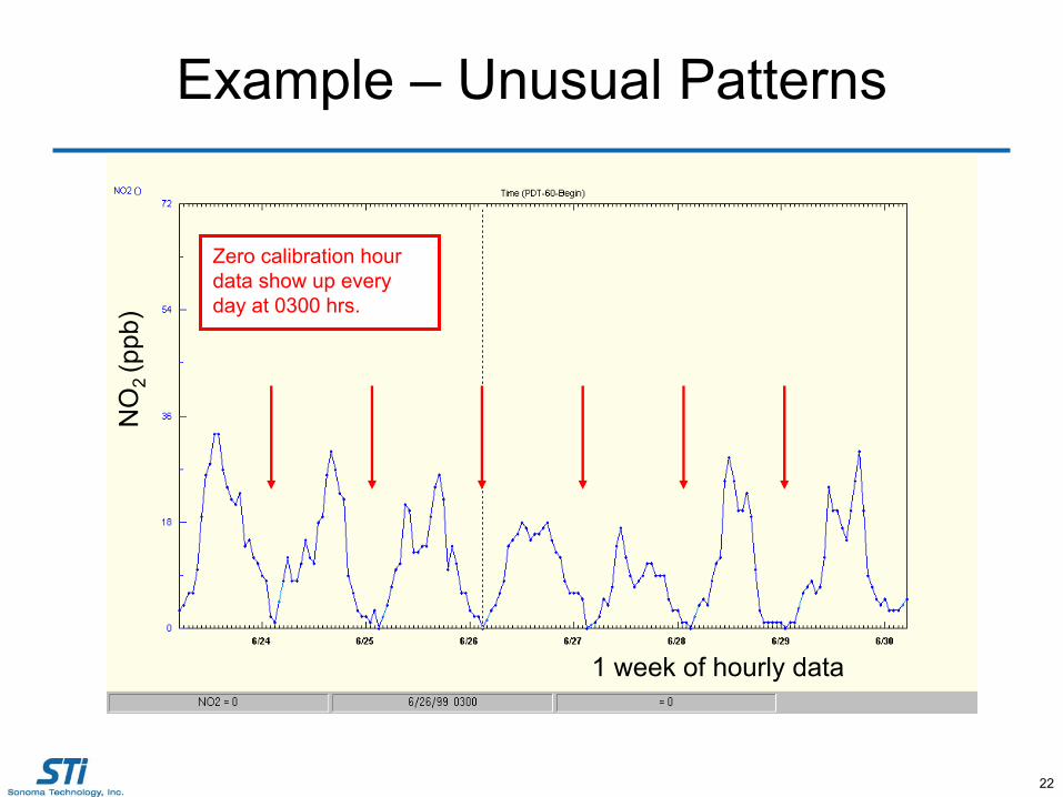
Example –

Unusual Patterns

Zero calibration hour data show up every day at 0300 hrs.

NO

2 (p

pb)

1 week of hourly data

23

Likely real “blip”

in NOand NOx

Example –

Ozone, NOx

, NO

24

Sample Screening Criteria Carbon Monoxide

•

Checks:–

Select buddy check criteria

•

Checks may vary with instrument sensitivity

Check Criteria

Maximum >15 ppm

Minimum –1 ppm

Rate of change >10 ppm/hr

Sticking check > 0 ppm for 5 hours

Co-pollutant NO, acetylene

26

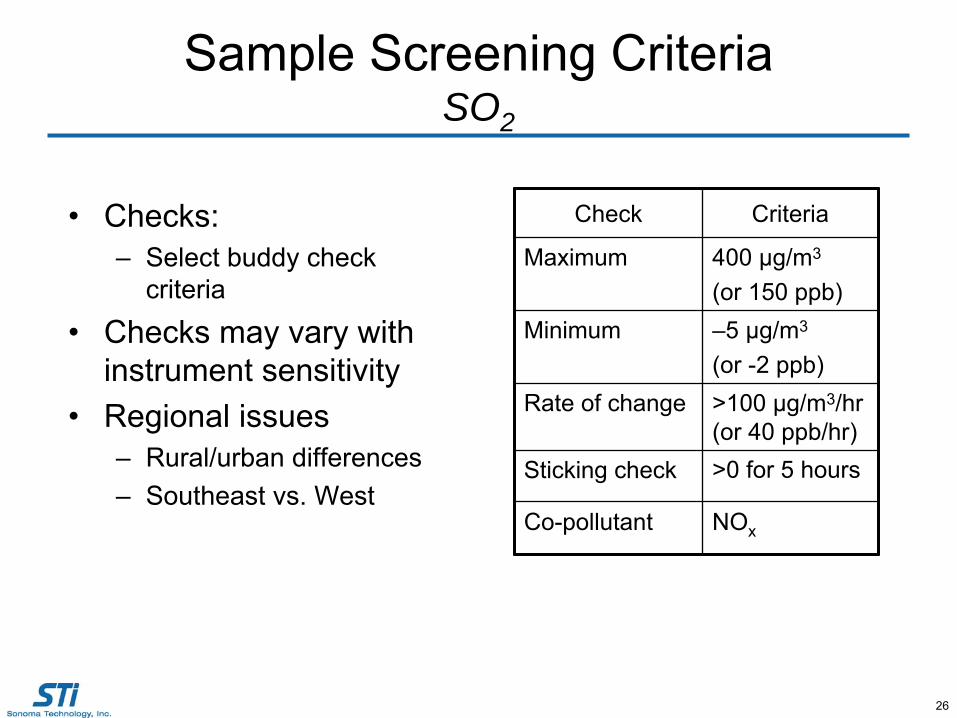
Sample Screening Criteria SO2

•

Checks:–

Select buddy check criteria

•

Checks may vary with instrument sensitivity

•

Regional issues–

Rural/urban differences–

Southeast vs. West

Check Criteria

Maximum 400 μg/m3

(or 150 ppb)Minimum –5 μg/m3

(or -2 ppb)Rate of change >100 μg/m3/hr

(or 40 ppb/hr)Sticking check >0 for 5 hours

Co-pollutant NOx

28

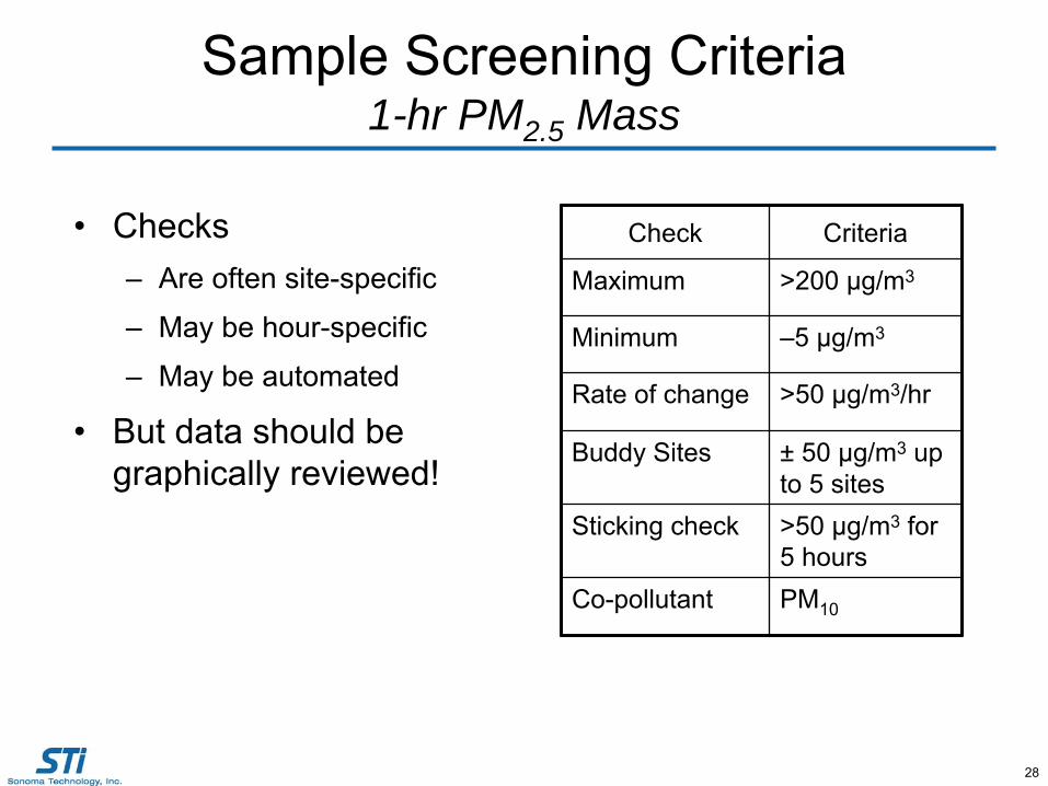
Sample Screening Criteria 1-hr PM2.5 Mass

•

Checks–

Are often site-specific

–

May be hour-specific

–

May be automated

•

But data should be graphically reviewed!

Check Criteria

Maximum >200 μg/m3

Minimum –5 μg/m3

Rate of change >50 μg/m3/hr

Buddy Sites ±

50 μg/m3

up to 5 sites

Sticking check >50 μg/m3

for 5 hours

Co-pollutant PM10

30

Example –

Wildfire Events

31

Los Angeles continuous PM2.5

mass concentrations on10/24/03 to 10/27/03 (raw data –

USEPA AIRNow)

High concentrations in the eastern part of the basin.

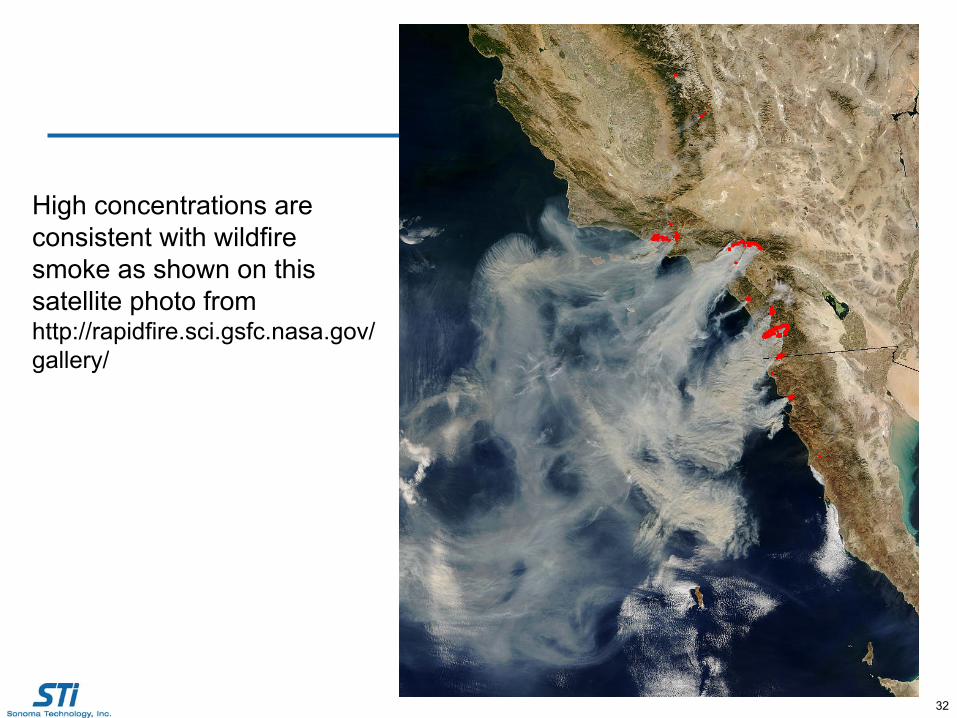
32

High concentrations are consistent with wildfire smoke as shown on this satellite photo from http://rapidfire.sci.gsfc.nasa.gov/

gallery/

33

Example –

Unusually Low ConcentrationsP

M2.

5m

ass

(μg/

m3 )

Possible interferencefrom moisture on the TEOM

Hourly PM2.5

Concentrations

34

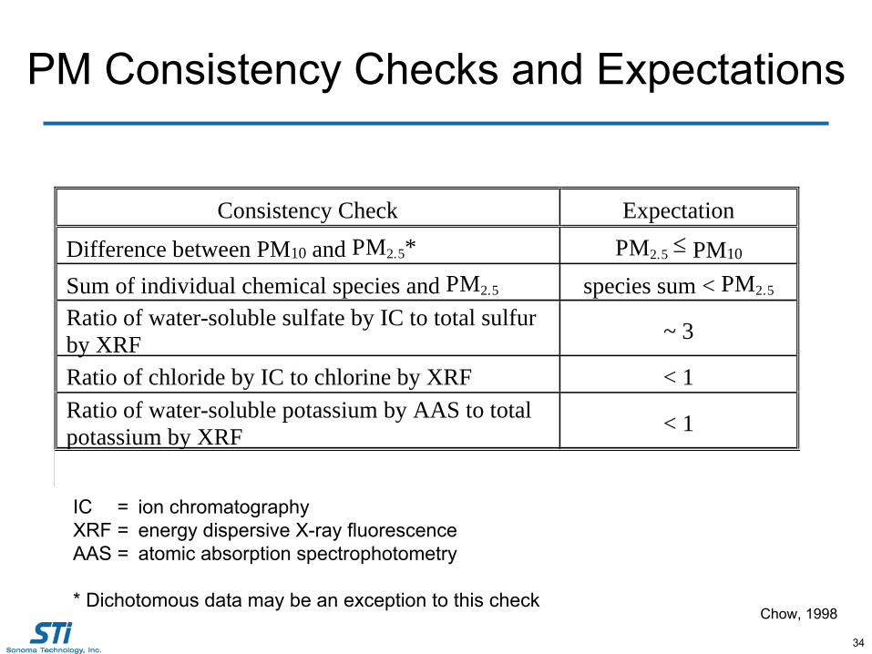
Consistency Check Expectation

Difference between PM10 and PM2.5* PM2.5 PM10

Sum of individual chemical species and PM2.5 species sum < PM2.5

Ratio of water-soluble sulfate by IC to total sulfurby XRF ~ 3

Ratio of chloride by IC to chlorine by XRF < 1Ratio of water-soluble potassium by AAS to totalpotassium by XRF < 1

babs compared to elemental carbon good correlation

PM Consistency Checks and Expectations

IC

=

ion chromatographyXRF

=

energy dispersive X-ray fluorescenceAAS

=

atomic absorption spectrophotometry

* Dichotomous data may be an exception to this checkChow, 1998

35

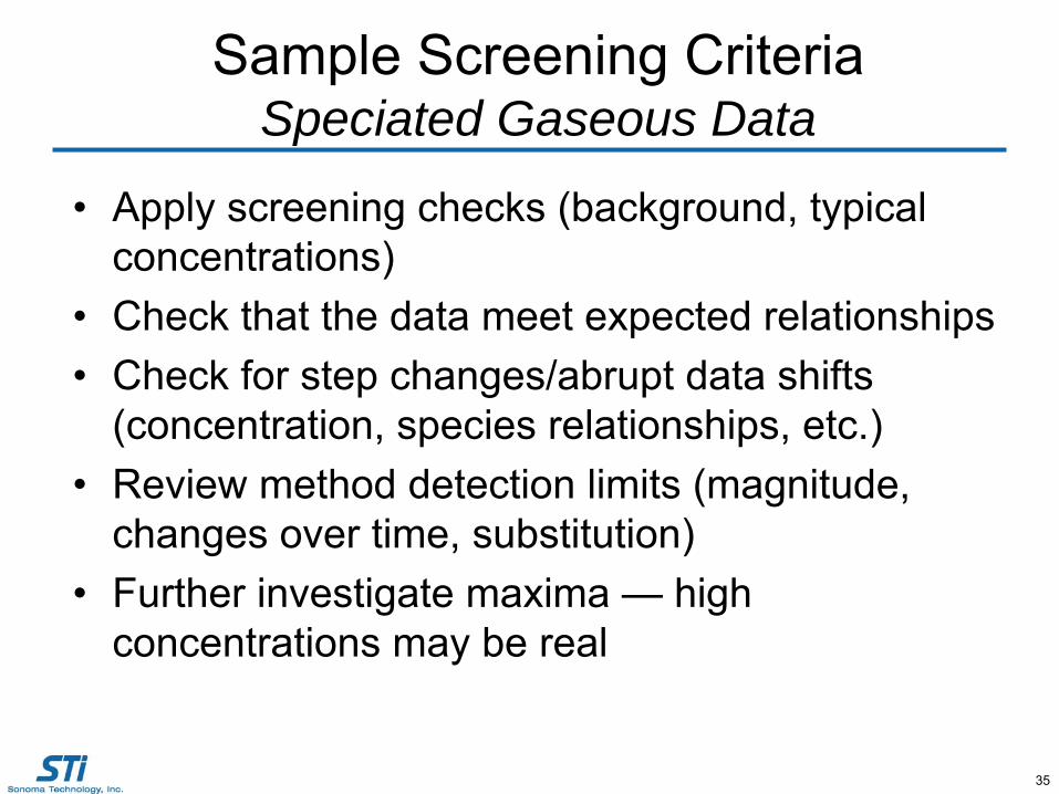
Sample Screening Criteria Speciated Gaseous Data

•

Apply screening checks (background, typical concentrations)

•

Check that the data meet expected relationships •

Check for step changes/abrupt data shifts (concentration, species relationships, etc.)

•

Review method detection limits (magnitude, changes over time, substitution)

•

Further investigate maxima —

high concentrations may be real

36

Concentrations (ppb) of carbon tetrachloride (CCl4), dichlorodifluoromethane (CCl2F2), and methyl chloride (CH3Cl) from 2003 and 2004.

0

0.2

0.4

0.6

0.8

1

3/10

/200

3

4/9/

2003

5/9/

2003

6/8/

2003

7/8/

2003

8/7/

2003

9/6/

2003

10/6

/200

3

11/5

/200

3

12/5

/200

3

1/4/

2004

2/3/

2004

3/4/

2004

Date

Con

cent

ratio

n (p

pb)

CCl2F2 CCl4 CH3Cl

CH3

Cl Background = 0.6 ppb

CCl2

F2

Background = 0.55 ppb

CCl4

Background = 0.09 ppb

Screening Data Using Remote Background Concentrations

•

Time series plot of concentrations of long-lived species compared to background concentrations measured at remote sites in the Northern Hemisphere.

•

Significant dips in concentrations are circled.

•

Concentrations more than 20% below the background level were identified as suspect for further review.

37

Concentration Spikes

Characterizing spikes requires significant work•

Identifying the spikes is straightforward using visual plots of the data (e.g., maps or time series).

•

Spikes caused by analytical or sampling error may indicate anomalous concentrations of other species.

•

Real spikes in ambient concentrations are likely due to nearby point sources.

•

A combination of maps, the Toxic Release Inventory, and local knowledge is likely required (but may not be sufficient) to explain spikes in ambient concentrations.

•

Fugitive emission/upsets data are needed (and may be difficult to obtain).

38

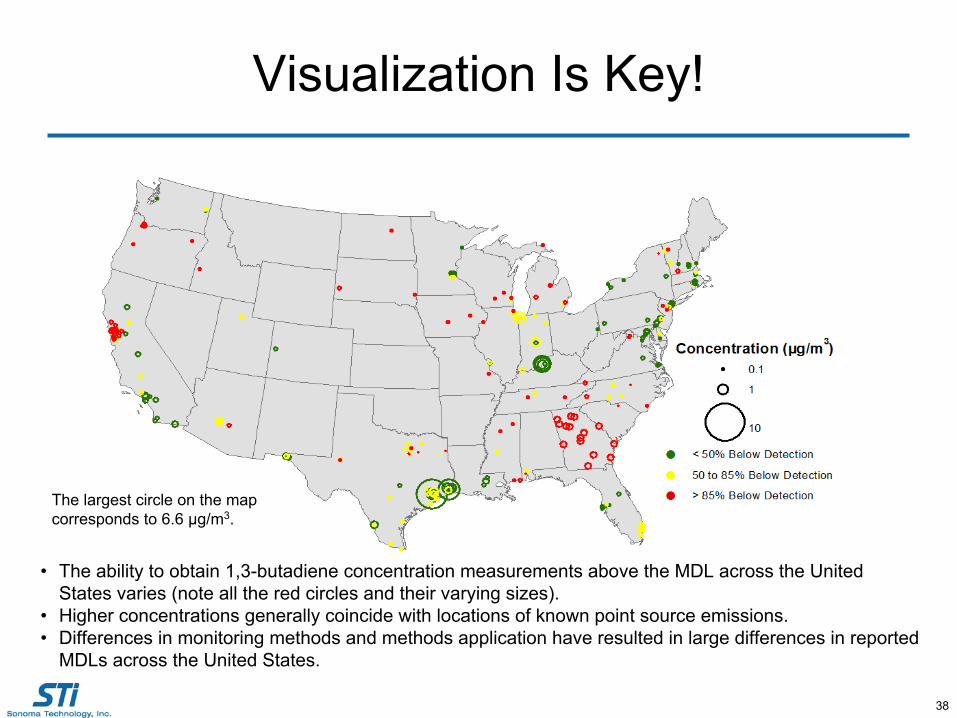
Visualization Is Key!

The largest circle on the map corresponds to 6.6 µg/m3.

•

The ability to obtain 1,3-butadiene concentration measurements above the MDL across the United States varies (note all the red circles and their varying sizes).

•

Higher concentrations generally coincide with locations of known

point source emissions.•

Differences in monitoring methods and methods application have resulted in large differences in reported MDLs across the United States.

39

Data Validation Summary

For pollutant data validation•

Understand formation, emissions, and transport

•

Establish and apply screening criteria to identify potentially suspect data

•

Investigate suspect data•

Invalidate data only if there is sufficient evidence

•

Document invalid data (so others can learn)

Data validation is very important!

40

Resources

•

Operator knowledge•

Previous documentation for the site and past data validation results

•

EPA guidance documents (available on AMTIC website)

•

Workbooks (e.g., Air Toxics, PAMS, and PM2.5

Data Analysis Workbooks)

•

Websites (e.g., IMPROVE, EPA Supersite)•

Journal articles and conference presentations (e.g., Atmospheric Environment, Environmental Science and Technology, Air and Waste Management Association)

•

Academia

41

Some Key Internet Sites•

Ambient Monitoring Technology Information Center: http://www.epa.gov/ttn/amtic/

•

IMPROVE QA/QC: http://vista.cira.colostate.edu/improve/Data/

QA_QC/qa_qc_Branch.htm•

EPA Quality Assurance: http://www.epa.gov/oar/oaqps/qa/index.html#back

•

EPA Supersite Overview: http://www.epa.gov/ttn/amtic/supersites.html

•

Air Toxics Data Analysis Workbook:http://www.epa.gov/ttnamti1/toxdat.html