Embed Size (px)
Citation preview
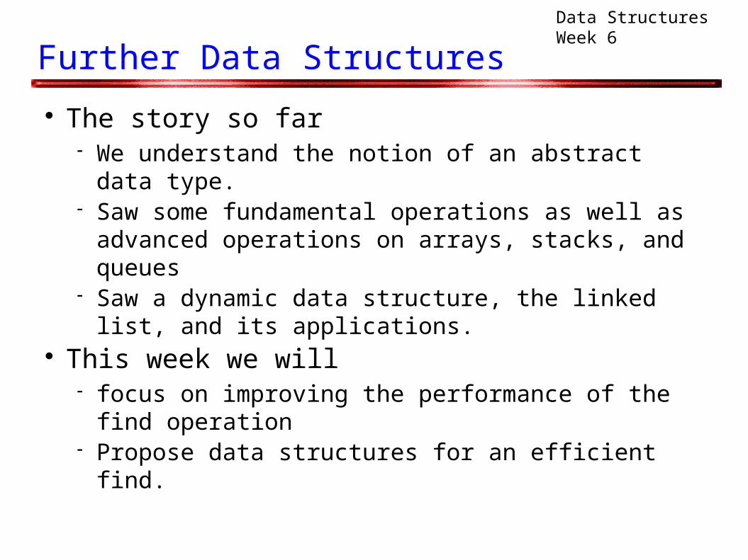
Data Structures Week 6
Further Data Structures
The story so far We understand the notion of an abstract data type. Saw some fundamental operations as well as advanced
operations on arrays, stacks, and queues Saw a dynamic data structure, the linked list, and its
applications. This week we will
focus on improving the performance of the find operation
Propose data structures for an efficient find.
Data Structures Week 6
Motivation
Consider a high-level programming language such
as C/C++. They need a compiler to translate the program into
assembly language and machine instructions. In that process, there are several processes and
several checks. One of them is to check for variable names, types,
etc. Ensure also that no duplicate names appear within
the same scope.
Data Structures Week 6
Motivation
Let us consider this duplicate variable names
problem. As we encounter a new variable declaration,
verify that in the same scope there are no other
declarations with the same name. If this is not a duplicate, need to store this name to
check future declarations. Once a scope is complete, can delete names from this
scope.
Data Structures Week 6
Motivation
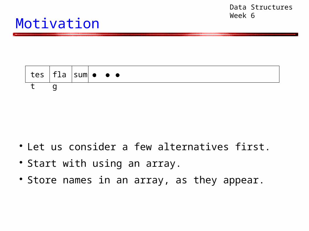
Let us consider a few alternatives first. Start with using an array. Store names in an array, as they appear.
test flag sum
Data Structures Week 6
Using an Array
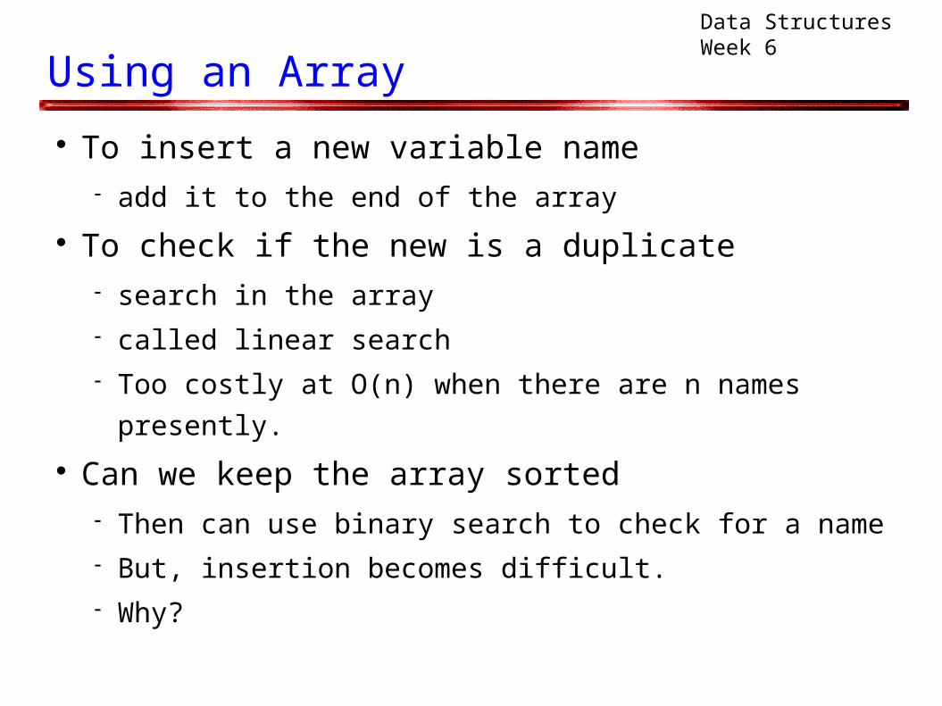
To insert a new variable name add it to the end of the array
To check if the new is a duplicate search in the array called linear search Too costly at O(n) when there are n names presently.
Can we keep the array sorted Then can use binary search to check for a name But, insertion becomes difficult. Why?
Data Structures Week 6
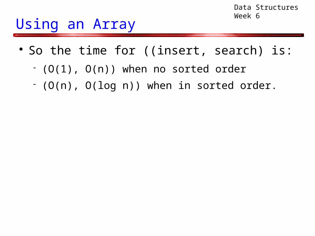
Using an Array
So the time for ((insert, search) is: (O(1), O(n)) when no sorted order (O(n), O(log n)) when in sorted order.
Data Structures Week 6
Using a Linked List
A linked list removes the drawback that the size
cannot grow dynamically. How would we use a linked list?
Data Structures Week 6
Using a Linked List
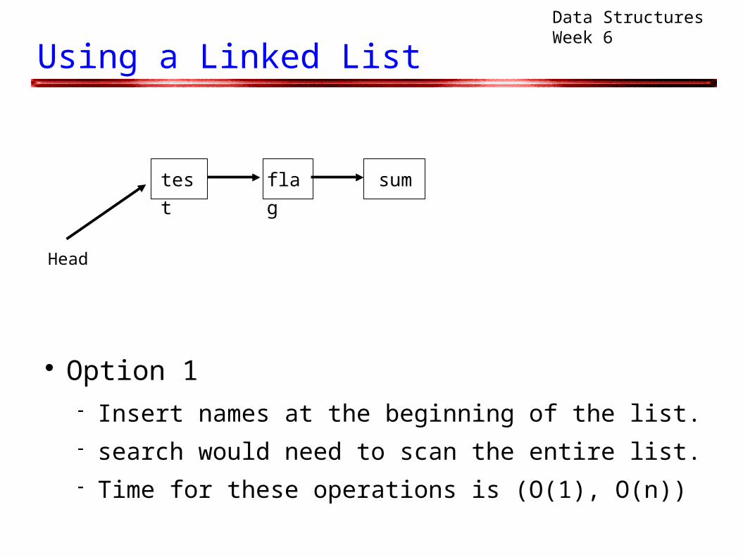
Option 1 Insert names at the beginning of the list. search would need to scan the entire list. Time for these operations is (O(1), O(n))
test flag sum
Head
Data Structures Week 6
Using a Linked List
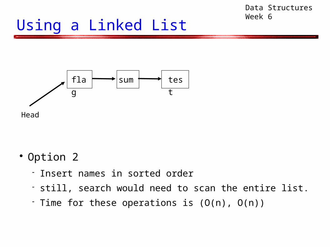
Option 2 Insert names in sorted order still, search would need to scan the entire list. Time for these operations is (O(n), O(n))
flag sum test
Head
Data Structures Week 6
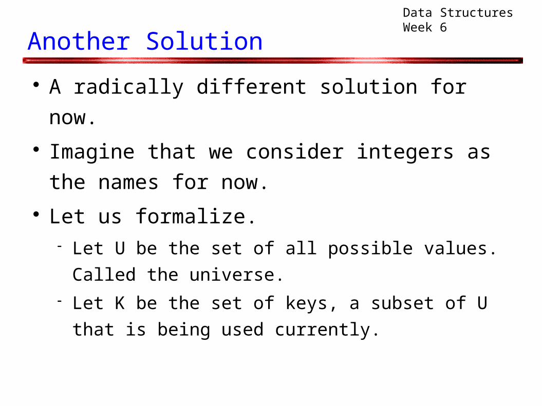
Another Solution
A radically different solution for now. Imagine that we consider integers as the names for
now. Let us formalize.
Let U be the set of all possible values. Called the
universe. Let K be the set of keys, a subset of U that is being
used currently.
Data Structures Week 6
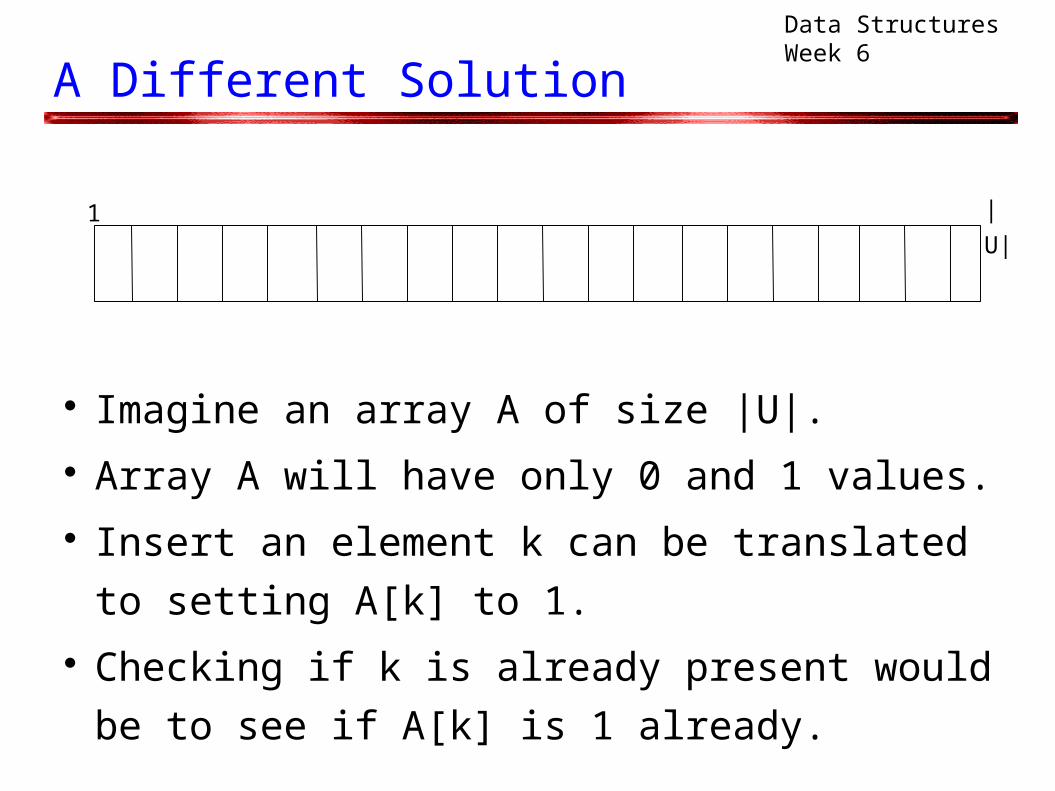
A Different Solution
Imagine an array A of size |U|. Array A will have only 0 and 1 values. Insert an element k can be translated to setting
A[k] to 1. Checking if k is already present would be to see if
A[k] is 1 already.
1 |U|
Data Structures Week 6
A Different Solution
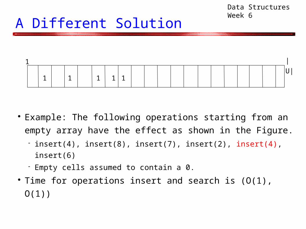
Example: The following operations starting from an
empty array have the effect as shown in the Figure. insert(4), insert(8), insert(7), insert(2), insert(4), insert(6) Empty cells assumed to contain a 0.
Time for operations insert and search is (O(1), O(1))
1 |U|
1 111 1
Data Structures Week 6
A Different Solution
has very good operation efficiency (++) But, can be very wasteful on space (---)
Imagine using such a solution for our original problem. Number of valid variable names > 268. Why? Number of variables in a typical program is about 100. So, we use only 100 cells of the array of size > 268.
Are there solutions so that insert, search time are
both small?
Data Structures Week 6
A New Data Structure
The drawback of the previous solution is that a lot
of space is reserved a-priori irrespective of usage. Our new solution will use a space only proportional
to the usage. Still will be based on arrays. Called a hash table. Details follow.

Data Structures Week 6
Hash Table
Consider an array T of size |T|. T is called a hash table
Consider a function h that maps elements in U to
the set {0, 1, ..., |T|-1}. h is called the hash function.
Can use the function h to map elements to indices. Details follow.
Data Structures Week 6
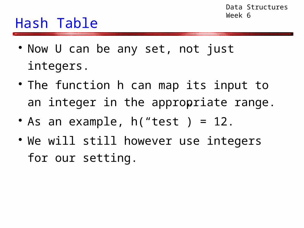
Hash Table
Now U can be any set, not just integers. The function h can map its input to an integer in
the appropriate range. As an example, h(“test”) = 12. We will still however use integers for our setting.
Data Structures Week 6
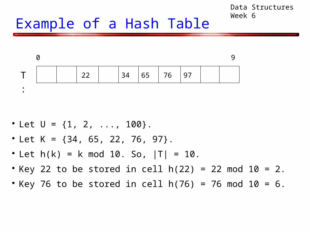
Example of a Hash Table
Let U = {1, 2, ..., 100}. Let K = {34, 65, 22, 76, 97}. Let h(k) = k mod 10. So, |T| = 10. Key 22 to be stored in cell h(22) = 22 mod 10 = 2. Key 76 to be stored in cell h(76) = 76 mod 10 = 6.
0 9
34 6522 76 97T :
Data Structures Week 6
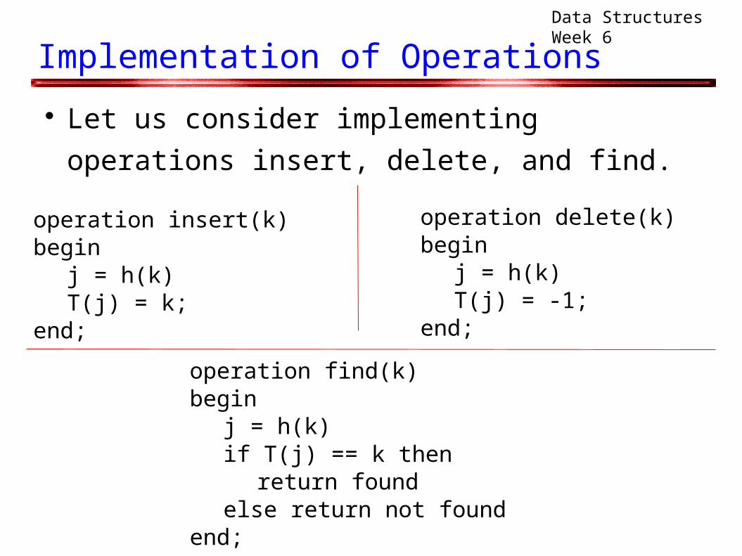
Implementation of Operations
Let us consider implementing operations insert,
delete, and find.
operation insert(k)begin
j = h(k)T(j) = k;
end;
operation delete(k)begin
j = h(k)T(j) = -1;
end;
operation find(k)begin
j = h(k)if T(j) == k then
return foundelse return not found
end;
Data Structures Week 6
Operations
Let us consider the runtime of these operations. All operations run in O(1) time.
Provided, certain conditions hold. What are these conditions?
Note the similarity to the array based solution
(Solution 3) Instead of accessing cell k, we now access cell h(k). But, instead of using a space of |U|, we use a space of
|T|.
Data Structures Week 6
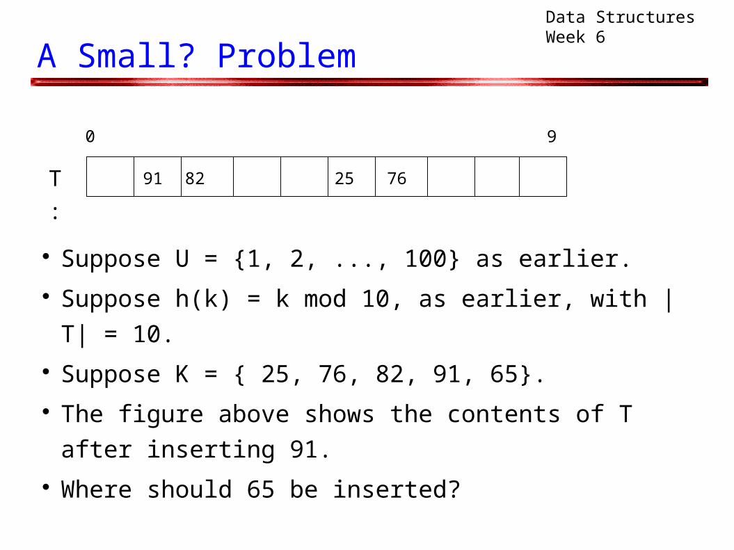
A Small? Problem
Suppose U = {1, 2, ..., 100} as earlier. Suppose h(k) = k mod 10, as earlier, with |T| = 10. Suppose K = { 25, 76, 82, 91, 65}. The figure above shows the contents of T after
inserting 91. Where should 65 be inserted?
0 9
2582 76T : 91
Data Structures Week 6
A Small? Problem
Notice that 65 is different from 25. So should store
both. But, each cell of the array T can store only one
element of U. How do we resolve this?
Data Structures Week 6
A Collision
The situation is termed as a collision. Can it be avoided?
Not completely. Notice that h maps elements of U to a range of size |T|. If |U| > |T|, cannot avoid collisions.
Can they be minimized? Certainly. Choosing h() carefully can minimize collisions. Some guidelines to choose h() are given next.
Data Structures Week 6
How to Choose the Hash Function?
TO DO
Data Structures Week 6
Collision Resolution
Despite careful efforts, it is very likely that
collisions exist. We should have a way to handle them properly. Such techniques are called collision resolution
techniques. We shall study some of those techniques.
Data Structures Week 6
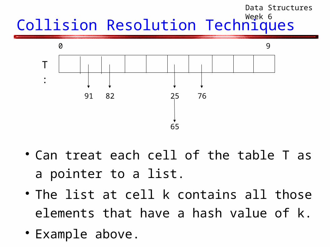
Collision Resolution Techniques
Can treat each cell of the table T as a pointer to a
list. The list at cell k contains all those elements that
have a hash value of k. Example above.
0 9
2582 76
T :
91
65
Data Structures Week 6
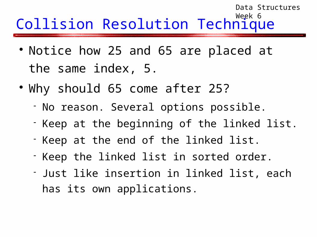
Collision Resolution Technique
Notice how 25 and 65 are placed at the same
index, 5. Why should 65 come after 25?
No reason. Several options possible. Keep at the beginning of the linked list. Keep at the end of the linked list. Keep the linked list in sorted order. Just like insertion in linked list, each has its own
applications.
Data Structures Week 6
Collision Resolution
The above technique is called chaining. Names comes from the fact that elements with the
same hash value are chained together in a linked
list. Let us see how operations should now be
implemented. Assuming that insert is at the front of the list.
Data Structures Week 6
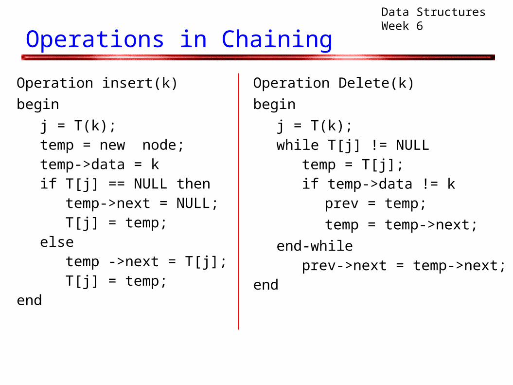
Operations in Chaining
Operation insert(k)
begin
j = T(k);temp = new node;temp->data = kif T[j] == NULL then
temp->next = NULL;T[j] = temp;
elsetemp ->next = T[j]; T[j] = temp;
end
Operation Delete(k)
begin
j = T(k);while T[j] != NULL
temp = T[j];if temp->data != k
prev = temp;
temp = temp->next;
end-whileprev->next = temp->next;
end
Data Structures Week 6
Operations in Chaining
Operation Find can be similarly implemented.
Data Structures Week 6
Analysis of the Operations
How to analyze the advantage of the solution? Consider a hash table using chaining to resolve
collisions. What is the runtime of insert and search?
Data Structures Week 6
Analysis of Operations
If we have a very bad hash function, h, then all
values may map to the same index. The list at that index will have all |K| = n elements. Now, find takes O(n) time, while insert can still be
done in O(1). What have we achieved?
Data Structures Week 6
Analysis of Operations
The above approach is too pessimistic. Need better analysis to analyze an average
scenario. Average scenario? Depends on the setting. In our setting, can imagine that
K can be a random subset of U. Still, very difficult to do average case analysis. Too many assumptions, too many unknowns.
Data Structures Week 6
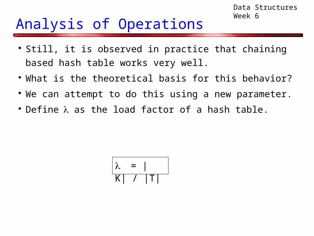
Analysis of Operations
Still, it is observed in practice that chaining based
hash table works very well. What is the theoretical basis for this behavior? We can attempt to do this using a new parameter. Define as the load factor of a hash table.
= |K| / |T|
Data Structures Week 6
Analysis Using How does help in our analysis? Assume the following
The hash function has the property that it hashes each
element of U to an element of T with equal probability. In other words, h is a uniform hash function. Does such a function exist?
Data Structures Week 6
Analysis Using With the above assumption on h
The expected number of elements in K that hash to a
given cell j = |K|/|T| = Can show the above using elementary random
variables. The above observation motivates the definition of .
Now, how do the runtime of insert and search
depend on .
Data Structures Week 6
Analysis Using For insert, since we insert at the beginning of the
list, it is always O(1). For search
Each chain is about elements long. If the element being searched for, say k, is not present,
the entire list will be searched for. This is called as an unsuccessful search.
If the element being searched for is present, We can stop the search once the element is found. Typically, this happens at the middle of the list. So need to search at least /2 elements. This is called as a successful search.
Data Structures Week 6
Other Approaches to Resolve Collisions
Problems with the chaining approach: use of pointers. Can become difficult to program and
verify. Cannot predict the state of the hash table easily. Can
keep on adding whereas a rehashing may be better. Slightly more space than |T|.
Some of these problems can be addressed.
Data Structures Week 6
Open Addressing
The technique is called open addressing. No additional space is used apart from the table T. So how to address a collision?
Try alternative cells in the table. Details follow.
Data Structures Week 6
Open Addressing
Recall that the hash function h maps elements in U
to indices in the table T. How can we have an alternative cell/index for a
key k? Idea: Use more hash functions.
Consider hash functions h1, h
2, ... all mapping U to
indices in T such that hi(k) = (h
i-1(k) + f(i)) mod |T|.
– f() is a function on N->N.
Data Structures Week 6
Open Addressing
Depending on the function f() several variations are
possible. We'll consider three choices.
Data Structures Week 6
Linear Probing
Consider the case when f(i) = 1.
When h0(k) = h(k) itself, we now have that
h1(k) = h0(k) + 1
h2(k) = h1(k) + 1
...
Suggesting that the next slots that are tried in
succession starting from the slot j = h(k) are j+1 j+2 .
Data Structures Week 6
Linear Probing
Notice that eventually all slots may be tried. When all slots are tried, this indicates that the table
T is full. Also, while the table is not full, an empty cell can
always be found.
Data Structures Week 6
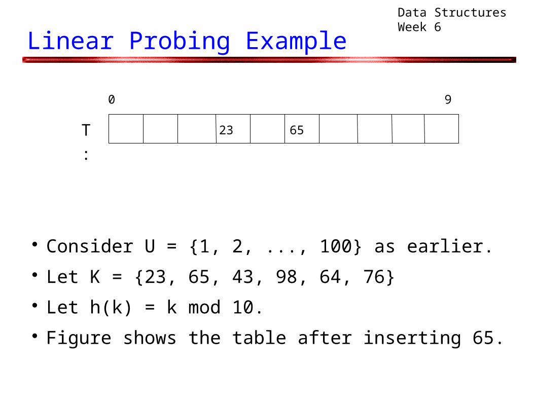
Linear Probing Example
Consider U = {1, 2, ..., 100} as earlier. Let K = {23, 65, 43, 98, 64, 76} Let h(k) = k mod 10. Figure shows the table after inserting 65.
0 9
6523T :
Data Structures Week 6
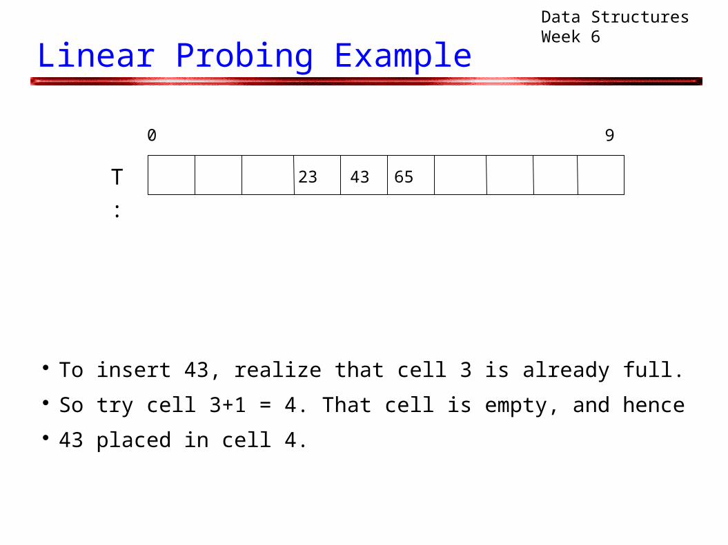
Linear Probing Example
To insert 43, realize that cell 3 is already full. So try cell 3+1 = 4. That cell is empty, and hence 43 placed in cell 4.
0 9
6523T : 43
Data Structures Week 6
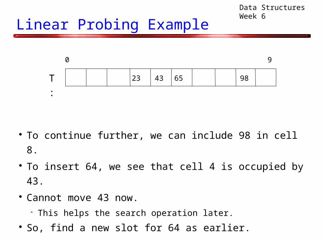
Linear Probing Example
To continue further, we can include 98 in cell 8. To insert 64, we see that cell 4 is occupied by 43. Cannot move 43 now.
This helps the search operation later.
So, find a new slot for 64 as earlier.
0 9
6523T : 43 98
Data Structures Week 6
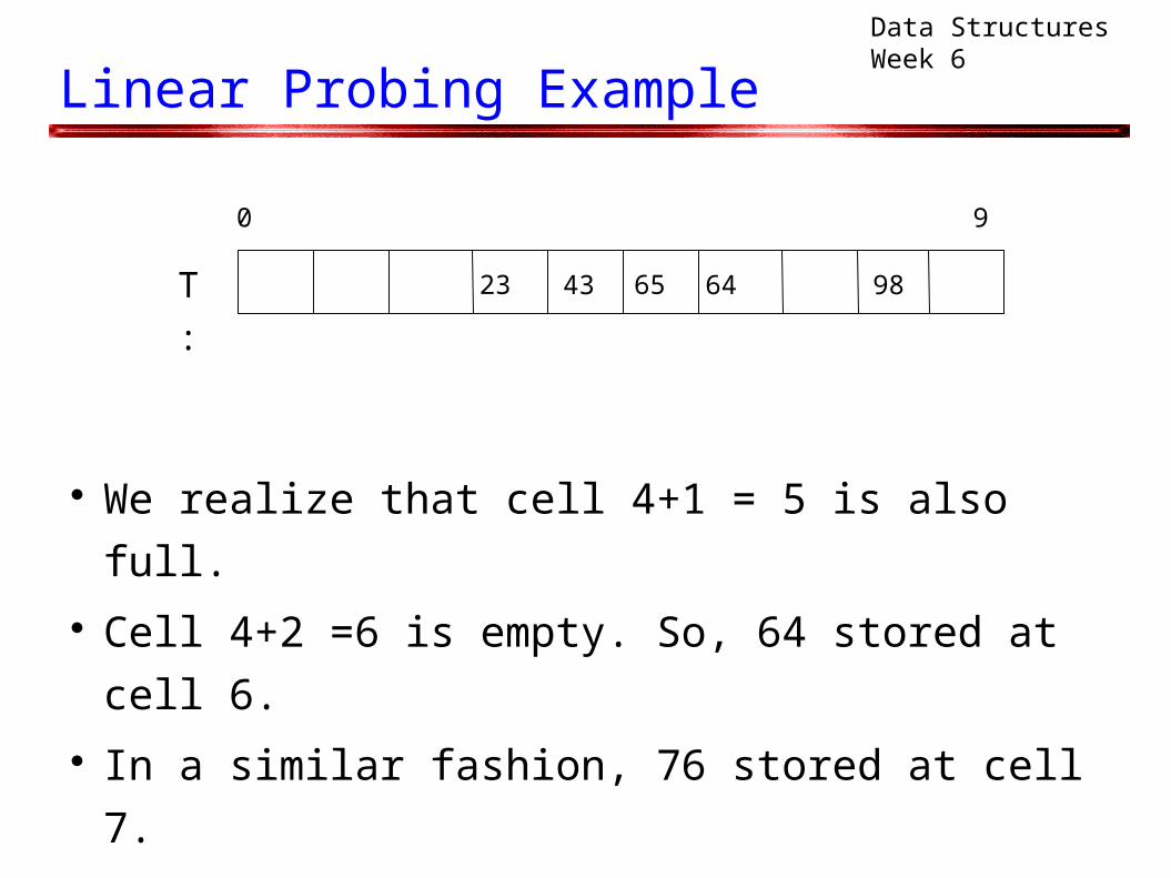
Linear Probing Example
We realize that cell 4+1 = 5 is also full. Cell 4+2 =6 is empty. So, 64 stored at cell 6. In a similar fashion, 76 stored at cell 7.
0 9
6523T : 43 9864
Data Structures Week 6
Linear Probing
The operation find(k) works similarly. Cannot declare k not found if T[h(k)] does not
contain k. We should search at indices h(k)+1, h(k)+2, ... How long?
A good quick question.
Data Structures Week 6
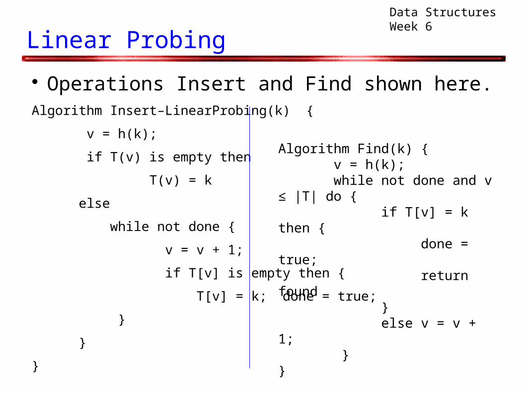
Linear Probing
Operations Insert and Find shown here.Algorithm Insert–LinearProbing(k) {
v = h(k);
if T(v) is empty then
T(v) = k
else
while not done {
v = v + 1;
if T[v] is empty then {
T[v] = k; done = true;
}
}
}
Algorithm Find(k) { v = h(k); while not done and v ≤ |T| do { if T[v] = k then { done = true; return found } else v = v + 1; }}
Data Structures Week 6
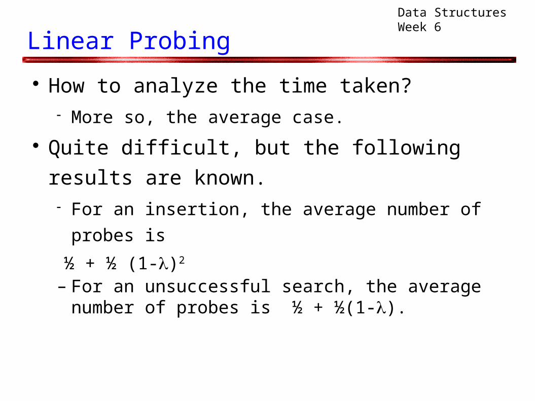
Linear Probing
How to analyze the time taken? More so, the average case.
Quite difficult, but the following results are known. For an insertion, the average number of probes is
½ + ½ (1-)2
– For an unsuccessful search, the average number of probes is ½ + ½(1-).

Data Structures Week 6
Linear Probing
A few issues with linear probing. Delete is a problem.
Affects searchability. Normally, a virtual delete option is used.
Another observation: The table may have areas
that are more dense compared to other areas. Reason for this is that inserts look for empty cells
linearly. This problem is called as primary clustering.
Data Structures Week 6
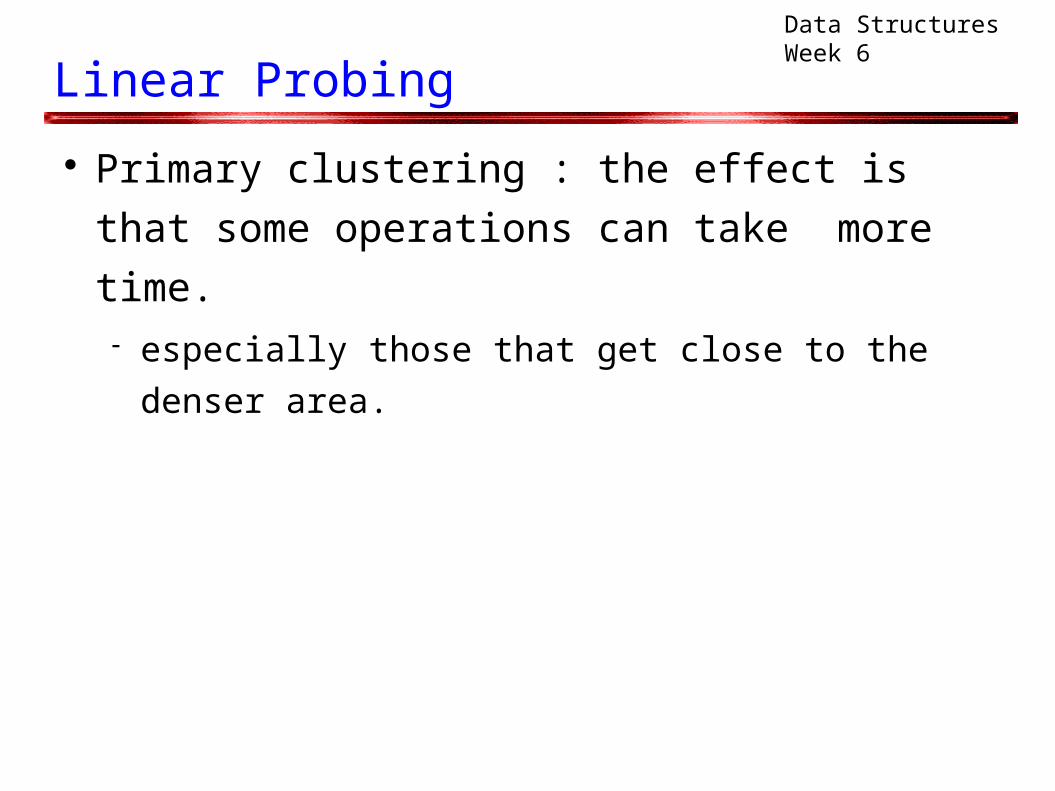
Linear Probing
Primary clustering : the effect is that some
operations can take more time. especially those that get close to the denser area.
Data Structures Week 6
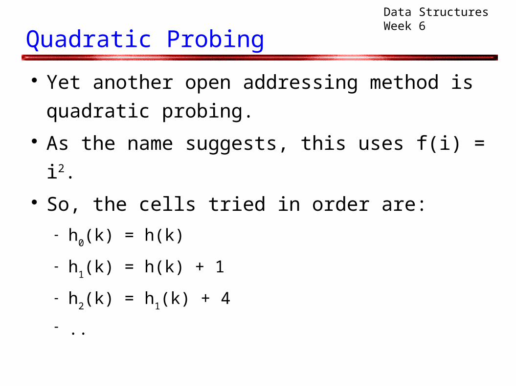
Quadratic Probing
Yet another open addressing method is quadratic
probing. As the name suggests, this uses f(i) = i2. So, the cells tried in order are:
h0(k) = h(k)
h1(k) = h(k) + 1
h2(k) = h1(k) + 4
..
Data Structures Week 6
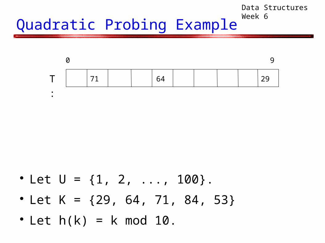
Quadratic Probing Example
Let U = {1, 2, ..., 100}. Let K = {29, 64, 71, 84, 53} Let h(k) = k mod 10.
0 9
T : 64 2971
Data Structures Week 6
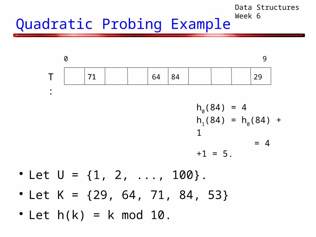
Quadratic Probing Example
Let U = {1, 2, ..., 100}. Let K = {29, 64, 71, 84, 53} Let h(k) = k mod 10.
0 9
71T : 64 29
h0(84) = 4
h1(84) = h
0(84) + 1
= 4 +1 = 5.
71 84
Data Structures Week 6
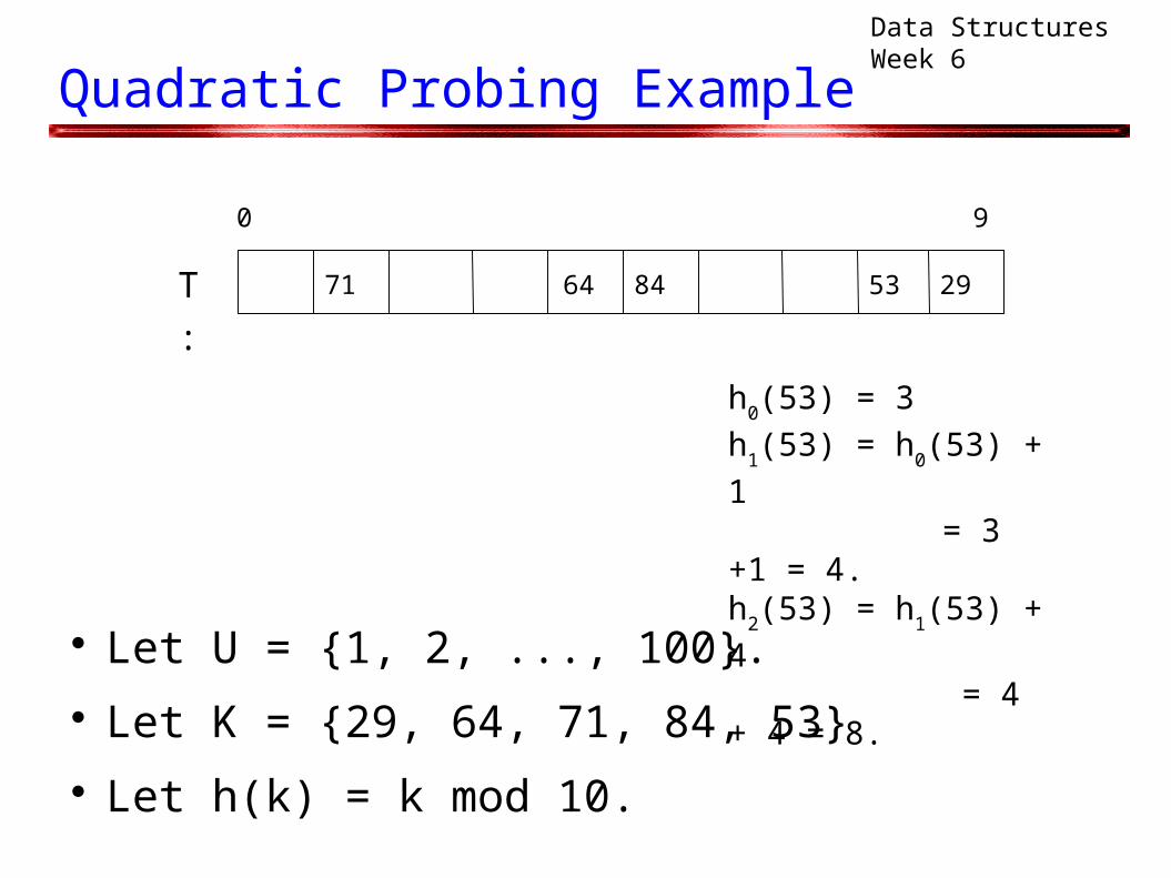
Quadratic Probing Example
Let U = {1, 2, ..., 100}. Let K = {29, 64, 71, 84, 53} Let h(k) = k mod 10.
0 9
84T : 64 29
h0(53) = 3
h1(53) = h
0(53) + 1
= 3 +1 = 4.h
2(53) = h
1(53) + 4
= 4 + 4 = 8.
5371
Data Structures Week 6
The Find Operation
How should it proceed? When can it stop?
Data Structures Week 6
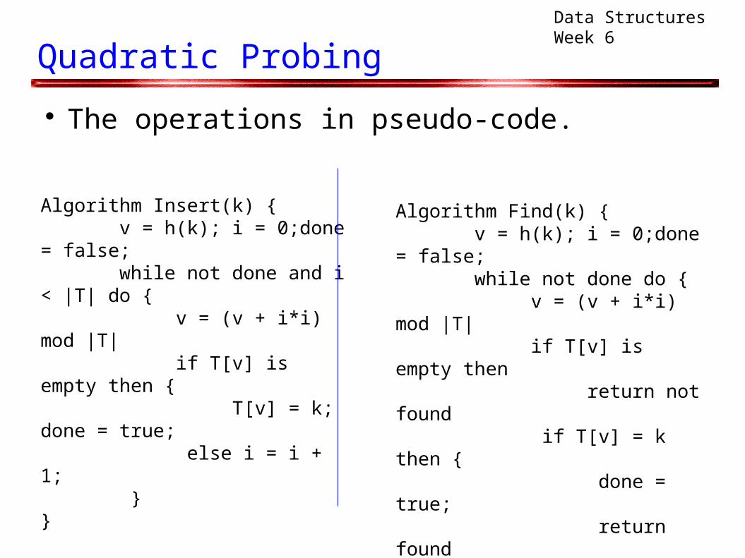
Quadratic Probing
The operations in pseudo-code.
Algorithm Find(k) { v = h(k); i = 0;done = false; while not done do { v = (v + i*i) mod |T| if T[v] is empty then return not found if T[v] = k then { done = true; return found } else i = i + 1; }}
Algorithm Insert(k) { v = h(k); i = 0;done = false; while not done and i < |T| do { v = (v + i*i) mod |T| if T[v] is empty then { T[v] = k; done = true; else i = i + 1; }}
Data Structures Week 6
Quadratic Probing
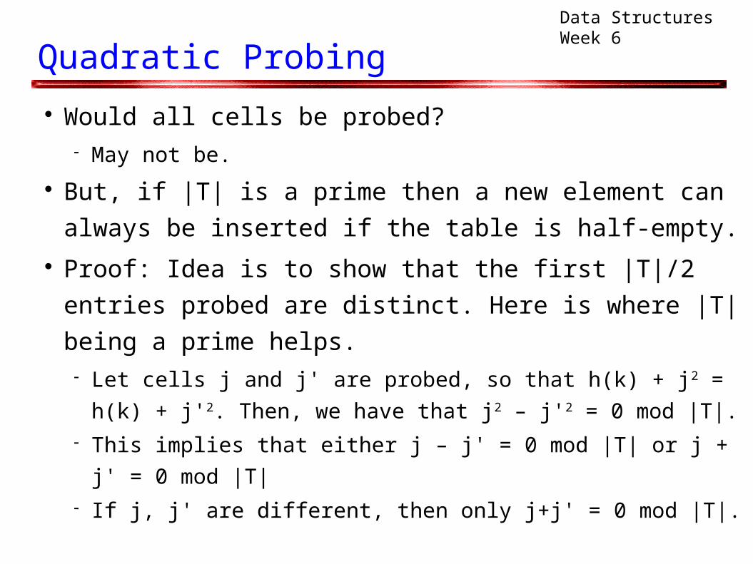
Would all cells be probed? May not be.
But, if |T| is a prime then a new element can always
be inserted if the table is half-empty. Proof: Idea is to show that the first |T|/2 entries probed
are distinct. Here is where |T| being a prime helps. Let cells j and j' are probed, so that h(k) + j2 = h(k) + j'2.
Then, we have that j2 – j'2 = 0 mod |T|. This implies that either j – j' = 0 mod |T| or j + j' = 0 mod |T| If j, j' are different, then only j+j' = 0 mod |T|.
Data Structures Week 6
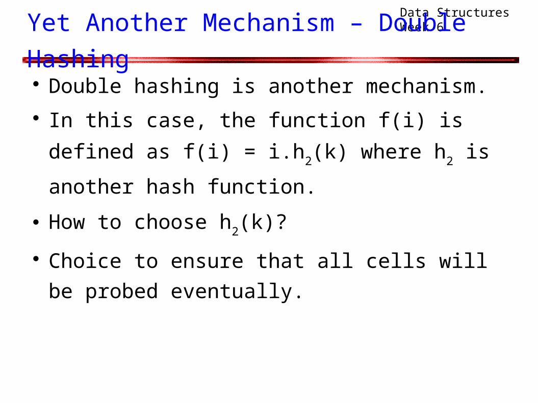
Yet Another Mechanism – Double Hashing
Double hashing is another mechanism. In this case, the function f(i) is defined as f(i) =
i.h2(k) where h
2 is another hash function.
How to choose h2(k)?
Choice to ensure that all cells will be probed
eventually.
Data Structures Week 6
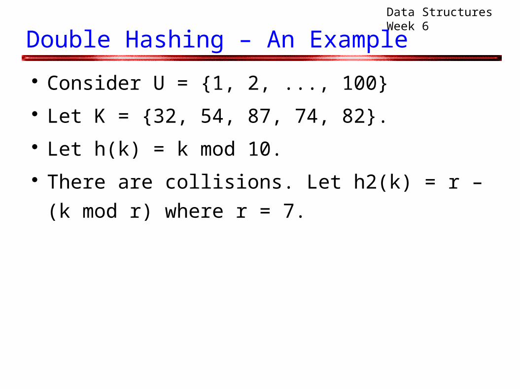
Double Hashing – An Example
Consider U = {1, 2, ..., 100} Let K = {32, 54, 87, 74, 82}. Let h(k) = k mod 10. There are collisions. Let h2(k) = r – (k mod r)
where r = 7.
Data Structures Week 6
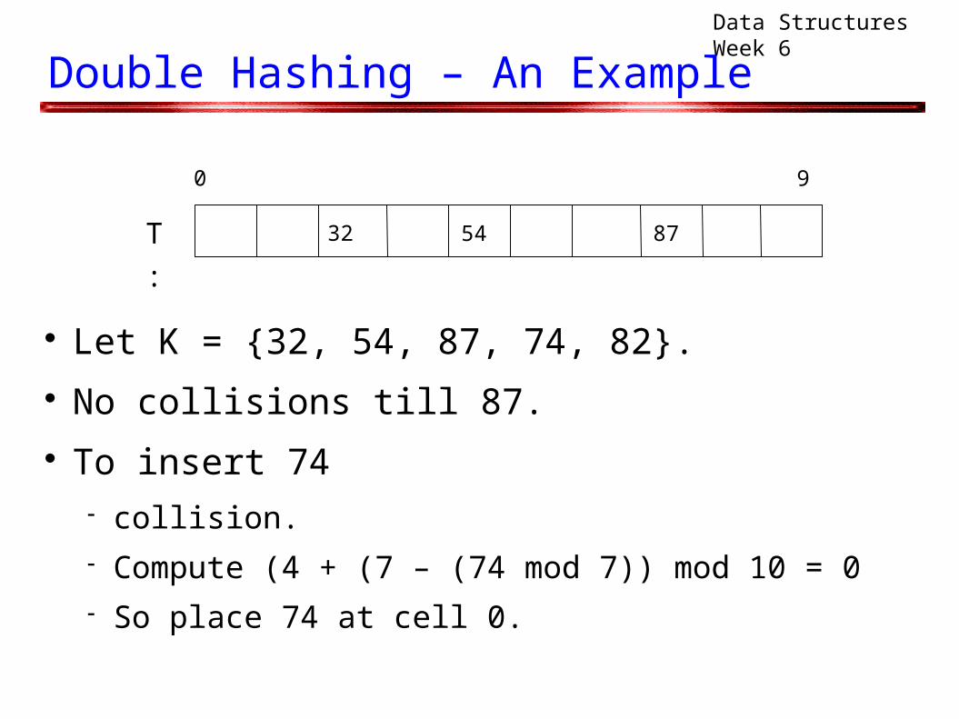
Double Hashing – An Example
Let K = {32, 54, 87, 74, 82}. No collisions till 87. To insert 74
collision. Compute (4 + (7 – (74 mod 7)) mod 10 = 0 So place 74 at cell 0.
0 9
32T : 54 87
Data Structures Week 6
Double Hashing – An Example
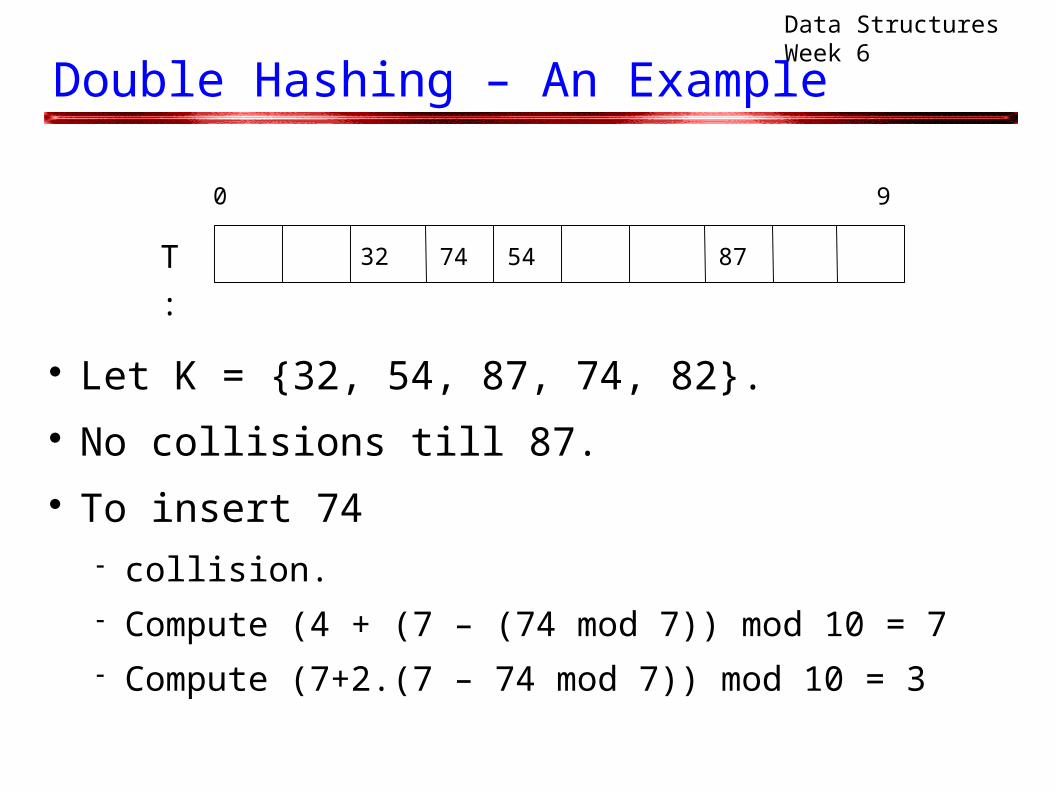
Let K = {32, 54, 87, 74, 82}. No collisions till 87. To insert 74
collision. Compute (4 + (7 – (74 mod 7)) mod 10 = 7 Compute (7+2.(7 – 74 mod 7)) mod 10 = 3
0 9
32T : 54 8774
Data Structures Week 6
Double Hashing – An Example
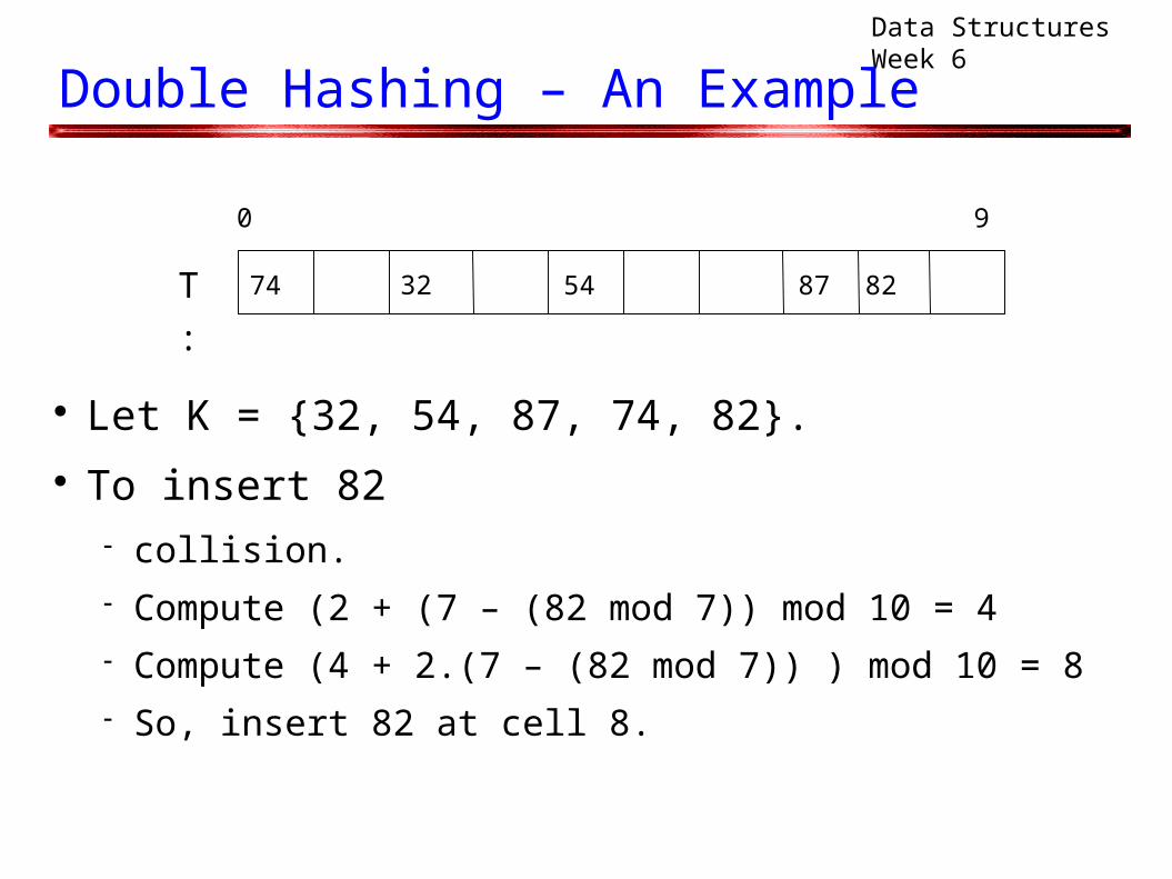
Let K = {32, 54, 87, 74, 82}. To insert 82
collision. Compute (2 + (7 – (82 mod 7)) mod 10 = 4 Compute (4 + 2.(7 – (82 mod 7)) ) mod 10 = 8 So, insert 82 at cell 8.
0 9
32T : 54 8774 82
Data Structures Week 6
Double Hashing
Can now write the routines for insert, search, etc.
Guidelines to choose h2(k)
h2(k) should never evaluate to 0.
ensure that all cells are probed.
Our earlier choice works well. In general, pick an r that is a prime and smaller than |T|
Define h2(k) = r – (k mod r).
Data Structures Week 6
Advanced Topics
For most of the techniques we discussed can only say that the average time is O(1), if lad factor
is O(1)
In some settings, can actually achieve a worst
case O(1) time. settings where the set of keys is known in advance.
This is called as universal hashing.