Data StructuresData Structures

Topic #12

Today’s Agenda• Sorting Algorithms

– insertion sort– selection sort– exchange sort– shell sort– radix sort

• As we learn about each sorting algorithm, we will discuss its efficiency

Sorting in General

• Sorting is the process that organizes collections of data into either ascending or descending order.

• Many of the applications you will deal with will require sorting; it is easier to understand data if it is organized numerically or alphabetically in order.

Sorting in General• As we found with the binary search,

– our data needs to be sorted to be able use more efficient methods of searching.

• There are two categories of sorting algs– Internal sorting requires that all of your data fit into

memory (an array or a LLL)

– External sorting is used when your data can't fit into memory all at once (maybe you have a very large database), and so sorting is done using disk files.

Sorting in General• Just like with searching,

– when we want to sort we need to pick from our data record the key to sort on (called the sort key).

– For example, if our records contain information about people, we might want to sort their names, id #s, or zip codes.

– Given a sorting algorithm, your entire table of information will be sorted based on only one field (the sort key).

Sorting in General

• The efficiency of our algorithms is dependent on the – number of comparisons we have to make with

our keys. – In addition, we will learn that sorting will also

depend on how frequently we must move items around.

Insertion Sort

• Think about a deck of cards for a moment.

• If you are dealt a hand of cards, imagine arranging the cards. – One way to put your cards in order is to pick one

card at a time and insert it into the proper position.

– The insertion sort acts just this way!

Insertion Sort

• The insertion sort divides the data into a sorted and unsorted region.

• Initially, the entire list is unsorted.

• Then, at each step, the insertion sort takes the first item of the unsorted region and places it into its correct position in the sorted region.

Insertion Sort

• Sort in class the following:– 29, 10, 14, 37, 13, 12, 30, 20

• Notice, the insertion sort uses the idea of keeping the first part of the list in correct order, once you've examined it.

• Now think about the first item in the list.• Using this approach, it is always considered

to be in order!

Insertion Sort

• Notice that with an insertion sort, even after most of the items have been sorted, – the insertion of a later item may require that you

move MANY of the numbers. – We only move 1 position at a time. – Thus, think about a list of numbers organized in

reverse order? How many moves do we need to make?

Insertion Sort• With the first pass,

– we make 1 comparison. – With the second pass, in the worst case we must make 2

comparisons. – With the third pass, in the worst case we must make 3

comparisons. – With the N-1 pass, in the worst case we must make N-1

comparisons. – In worst case: 1 + 2 + 3 + ... + (N-1)– which is: N*(N-1)/2 O(N2)

Insertion Sort

• But, how does the “direction” of comparison change this worst case situation?– if the list is already sorted and we compare left

to right, vs. right to left– if the list is exactly in the opposite order?– how would this change if the data were stored

in a linear linked list instead of an array?

Insertion Sort

• In addition, the algorithm moves data at most the same number of times.– So, including both comparisons and

exchanges, we get N(N-1) = N*N - N

• This can be summarized as a O(N2) algorithm in the worst case. – We should keep in mind that this means as our

list grows larger the performance will be dramatically reduced.

Insertion Sort

• For small arrays - fewer than 50 - the simplicity of the insertion sort makes it a reasonable approach.

• For large arrays -- it can be extremely inefficient!

• However, if your data is close to being sorted and a right->left comparison method is used, with LLL this can be greatly improved

Selection Sort• Imagine the case where we can look at all of

the data at once...and to sort it...find the largest item and put it in its correct place.

• Then, we find the second largest and put it in its place, etc.

• If we were to think about cards again, – it would be like looking at our entire hand of

cards and ordering them by selecting the largest first and putting at the end, and then selecting the rest of the cards in order of size.

Selection Sort• This is called a selection sort.

– It means that to sort a list, we first need to search for the largest key.

– Because we will want the largest key to be at the last position, we will need to swap the last item with the largest item.

• The next step will allow us to ignore the last (i.e., largest) item in the list. – This is because we know that it is the largest item...we

don't have to look at it again or move it again!

Selection Sort• So, we can once again search for the largest

item...in a list one smaller than before.

• When we find it, we swap it with the last item (which is really the next to the last item in the original list).

• We continue doing this until there is only 1 item left.

Selection Sort• Sort in class the following:

– 29, 10, 14, 37, 13, 12, 30, 20

• Notice that the selection sort doesn't require as many data moves as Insertion Sort.

• Therefore, if moving data is expensive (i.e., you have large structures), a selection sort would be preferable over an insertion sort.

Selection Sort

• Selection sort requires both comparisons and exchanges (i.e., swaps). – Start analyzing it by counting the number of

comparisons and exchanges for an array of N elements.

– Remember the selection sort first searches for the largest key and swaps the last item with the largest item found.

Selection Sort• Remember that means for the first time

around there would be N-1 comparisons. – The next time around there would be N-2

comparisons (because we can exclude comparing the previously found largest! Its already in the correct spot!).

– The third time around there would be N-3 comparisons.

– So...the number of comparisons would be:(N-1)+(N-2)+...+ 1 = N*(N-1)/2

Selection Sort• Next, think about exchanges.

• Every time we find the largest...we perform a swap.

• This causes 3 data moves (3 assignments).

• This happens N-1 times!

• Therefore, a selection sort of N elements requires 3*(N-1) moves.

Selection Sort• Lastly, put all of this together:N*(N-1)/2 + 3*(N-1)• which is: N*N/2 - N/2 + 6N/2 - 3• which is: N*N/2 + 5N/2 - 3• Put this in perspective of what we learned

about with the BIG O method:1/2 N*N + O(N)

• Or, O(N2)

Selection Sort• Given this, we can make a couple of

interesting observations. – The efficiency DOES NOT depend on the initial

arrangement of the data. – This is an advantage of the selection sort. – However, O(N2) grows very rapidly, so the

performance gets worse quickly as the number of items to sort increases.

Selection Sort• Also notice that even with O(N2) comparisons there

are only O(N) moves. – Therefore, the selection sort could be a good choice over

other methods when data moves are costly but comparisons are not.

– This might be the case when each data item is large (i.e., big structures with lots of information) but the key is short.

– Of course, don't forget that storing data in a linked list allows for very inexpensive data moves for any algorithm!

Exchange Sort (Bubble sort)

• Many of you should already be familiar with the bubble sort. – It is used here as an example, but it is not a

particular good algorithm!

• The bubble sort simply compares adjacent elements and exchanges them if they are out of order.

• To do this, you need to make several passes over the data.

Exchange Sort (Bubble sort)• During the first pass, you compare the first

two elements in the list. – If they are out of order, you exchange them. – Then you compare the next pair of elements

(positions 2 and 3). – If they are out of order, you exchange them. – This algorithm continues comparing and

exchanging pairs of elements until you reach the end of the list.

Exchange Sort (Bubble sort)• Notice that the list is not sorted after this first

pass. – We have just "bubbled" the largest element up to

its proper position at the end of the list! – During the second pass, you do the exact same

thing....but excluding the largest (last) element in the array since it should already be in sorted order.

– After the second pass, the second largest element in the array will be in its proper position (next to the last position).

Exchange Sort (Bubble sort)

• In the best case, when the data is already sorted, only 1 pass is needed and only N-1 comparisons are made (with no exchanges).

• Sort in class the following:– 29, 10, 14, 37, 13, 12, 30, 20

• The bubble sort also requires both comparisons and exchanges (i.e., swaps).

Exchange Sort (Bubble sort)

• Remember, the bubble sort simply compares adjacent elements and exchanges them if they are out of order.

• To do this, you need to make several passes over the data.

• This means that the bubble sort requires at most N-1 passes through the array.

Exchange Sort (Bubble sort)

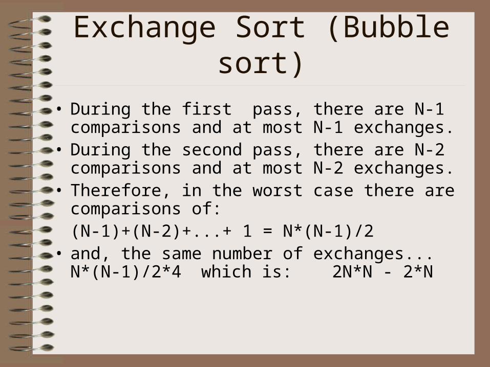
• During the first pass, there are N-1 comparisons and at most N-1 exchanges.

• During the second pass, there are N-2 comparisons and at most N-2 exchanges.

• Therefore, in the worst case there are comparisons of:

(N-1)+(N-2)+...+ 1 = N*(N-1)/2• and, the same number of exchanges... N*(N-1)/2*4

which is: 2N*N - 2*N

Exchange Sort (Bubble sort)

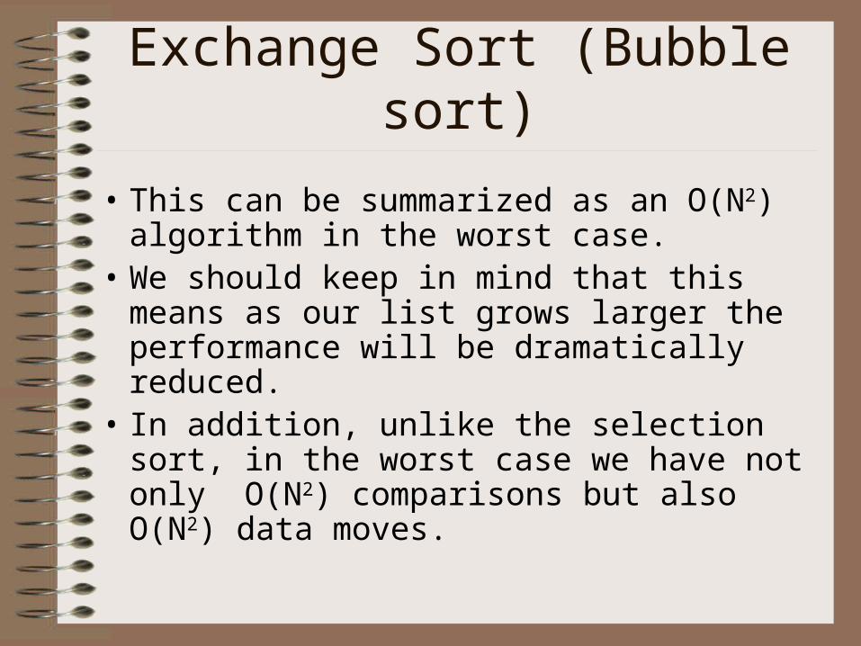
• This can be summarized as an O(N2) algorithm in the worst case.

• We should keep in mind that this means as our list grows larger the performance will be dramatically reduced.

• In addition, unlike the selection sort, in the worst case we have not only O(N2) comparisons but also O(N2) data moves.

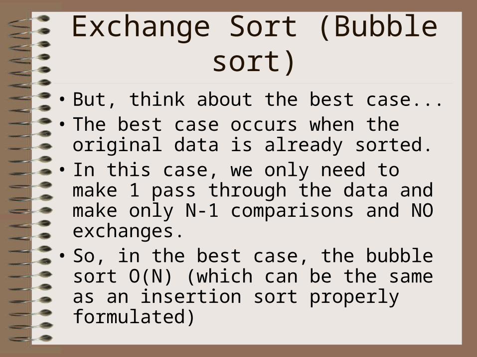
Exchange Sort (Bubble sort)• But, think about the best case...• The best case occurs when the original data

is already sorted. • In this case, we only need to make 1 pass

through the data and make only N-1 comparisons and NO exchanges.

• So, in the best case, the bubble sort O(N) (which can be the same as an insertion sort properly formulated)

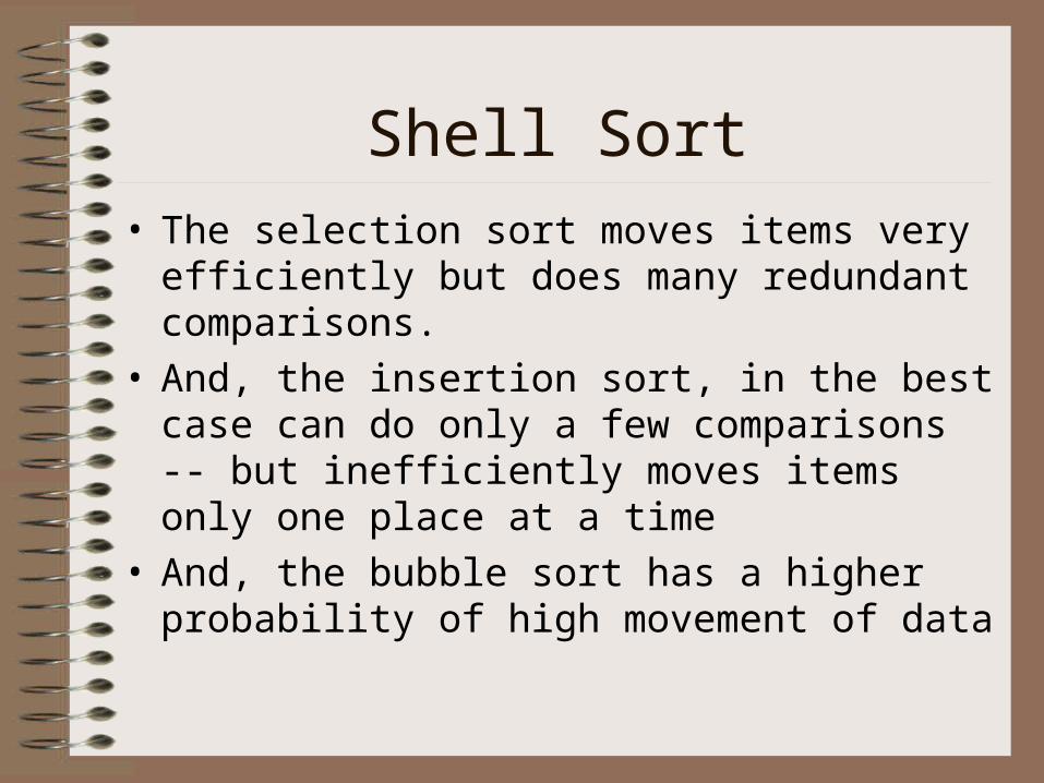
Shell Sort• The selection sort moves items very efficiently but

does many redundant comparisons. • And, the insertion sort, in the best case can do only

a few comparisons -- but inefficiently moves items only one place at a time

• And, the bubble sort has a higher probability of high movement of data

Shell Sort

• The shell sort is similar to the insertion sort, except it solves the problem of moving the items only one step at a time.

• The idea with the shell sort is to compare keys that are farther apart, and then resort a number of times, until you finally do an insertion sort

• We use “increments” to compare sets of data to essentially preprocess the data

Shell Sort

• With the shell sort you can choose any increment you want. – Some, however, work better than others. – A power of 2 is not a good idea. – Powers of 2 will compare the same keys on

multiple passes...so pick numbers that are not multiples of each other.

– It is a better way of comparing new information each time.

Shell Sort

• Sort in class the following:– 29, 10, 14, 37, 13, 12, 30, 20, 50, 5, 75, 11

• Try increments of 5, 3, and 1

• The final increment must always be 1

Radix Sort• Imagine that we are sorting a hand of cards.• This time, you pick up the cards one at a

time and arrange them by rank into 13 possible groups -- in the order 2,3,...10,J,Q,K,A.

• Combine each group face down on the table..so that the 2's are on top with the aces on bottom.

Radix Sort

• Pick up one group at a time and sort them by suit: clubs, diamonds, hearts, and spades.

• The result is a totally sorted hand of cards.

• The radix sort uses this idea of forming groups and then combining them to sort a collection of data.

Radix Sort• Look at an example using character strings:

• ABC, XYZ, BWZ, AAC, RLT, JBX, RDT, KLT, AEO, TLJ

• The sort begins by organizing the data according to the rightmost (least significant) letter and placing them into six groups in this case (do this in class)

Radix Sort

• Now, combine the groups into one group like we did the hand of cards.

• Take the elements in the first group (in their original order) and follow them by elements in the second group, etc.

• Resulting in:

• ABC, AAC, TLJ, AEO, RLT, RDT, KLT, JBX, XYZ, BWZ

Radix Sort• The next step is to do this again, using the

next letter (do this in class)• Doing this we must keep the strings

within each group in the same relative order as the previous result.

• Next, we again combine these groups into one result:

• AAC, ABC, JBX, RDT, AEO, TLJ, RLT, KLT, BWZ, XYZ

Radix Sort

• Lastly, we do this again, organizing the data by the first letter

• We do a final combination of these groups, resulting in:

• AAC, ABC, AEO, BWZ, JBX, KLT, RDT, RLT, TLJ , XYZ

• The strings are now in sorted order!– When working with strings of varying length, you

can treat them as if the short ones are padded on the right with blanks.

Radix Sort

• Notice just from this pseudo code that the radix sort requires N moves each time it forms groups and N moves to combine them again into one group.

• This algorithm performs 2*N moves "Digits" times.

• Notice that there are no comparisons!

Radix Sort• Therefore, at first glimpse, this method

looks rather efficient. – However, it does require large amounts of

memory to handle each group if implemented as an array.

– Therefore, a radix sort is more appropriate for a linked list than for an array.

– Also notice that the worst case and the average case (or even the best case) all will take the same number of moves.