Embed Size (px)
DESCRIPTION
Overview And Details Of Data Structure and Algorithm . Help To Reading and learning The Concept Of Data Structure and Algorithm.
Citation preview
Data Structure & Algorithms Data Structures are the programmatic way of storing data so that data can
be used efficiently. Almost every enterprise application uses various types
of data structures in one or other way. This tutorial will give you great
understanding on Data Structures concepts needed to understand the
complexity of enterprise level applications and need of algorithms, data
structures.
What is a Data Structure? Data Structure is a systematic way to organize data in order to use it
efficiently. Following terms are foundation terms of a data structure.
Interface − Each data structure has an interface. Interface represents the set
of operations that a data structure supports. An interface only provides the list
of supported operations, type of parameters they can accept and return type of
these operations.
Implementation − Implementation provides the internal representation of a
data structure. Implementation also provides the definition of the algorithms
used in the operations of the data structure.
Characteristics of a Data Structure Correctness − Data Structure implementation should implement its interface
correctly.
Time Complexity − Running time or execution time of operations of data
structure must be as small as possible.
Space Complexity − Memory usage of a data structure operation should be as
little as possible.
Need for Data Structure As applications are getting complex and data rich, there are three common
problems applications face now-a-days.
Parde
ep V
ats
Data Search − Consider an inventory of 1 million(106) items of a store. If
application is to search an item. It has to search item in 1 million(106) items
every time slowing down the search. As data grows, search will become slower.
Processor speed − Processor speed although being very high, falls limited if
data grows to billion records.
Multiple requests − As thousands of users can search data simultaneously on
a web server,even very fast server fails while searching the data.
To solve above problems, data structures come to rescue. Data can be
organized in a data structure in such a way that all items may not be
required to be search and required data can be searched almost instantly.
Execution Time Cases There are three cases which are usual used to compare various data
structure's execution time in relative manner.
Worst Case − This is the scenario where a particular data structure operation
takes maximum time it can take. If a operation's worst case time is ƒ(n) then
this operation will not take time more than ƒ(n) time where ƒ(n) represents
function of n.
Average Case − This is the scenario depicting the average execution time of an
operation of a data structure. If a operation takes ƒ(n) time in execution then m
operations will take mƒ(n) time.
Best Case − This is the scenario depicting the least possible execution time of
an operation of a data structure. If a operation takes ƒ(n) time in execution
then actual operation may take time as random number which would be
maximum as ƒ(n).
Parde
ep V
ats

Basic Terminology Data − Data are values or set of values.
Data Item − Data item refers to single unit of values.
Group Items − Data item that are divided into sub items are called as Group
Items.
Elementary Items − Data item that cannot be divided are called as
Elementary Items.
Attribute and Entity − An entity is that which contains certain attributes or
properties which may be assigned values.
Entity Set − Entities of similar attributes form an entity set.
Field − Field is a single elementary unit of information representing an attribute
of an entity.
Record − Record is a collection of field values of a given entity.
File − File is a collection of records of the entities in a given entity set.
Parde
ep V
ats
Data Structures - Algorithms Basics Algorithm is a step by step procedure, which defines a set of instructions to
be executed in certain order to get the desired output. Algorithms are
generally created independent of underlying languages, i.e. an algorithm
can be implemented in more than one programming language.
From data structure point of view, following are some important categories
of algorithms −
Search − Algorithm to search an item in a datastructure.
Sort − Algorithm to sort items in certain order
Insert − Algorithm to insert item in a datastructure
Update − Algorithm to update an existing item in a data structure
Delete − Algorithm to delete an existing item from a data structure
Characteristics of an Algorithm Not all procedures can be called an algorithm. An algorithm should have the
below mentioned characteristics −
Unambiguous − Algorithm should be clear and unambiguous. Each of its steps
(or phases), and their input/outputs should be clear and must lead to only one
meaning.
Input − An algorithm should have 0 or more well defined inputs.
Output − An algorithm should have 1 or more well defined outputs, and should
match the desired output.
Finiteness − Algorithms must terminate after a finite number of steps.
Feasibility − Should be feasible with the available resources.
Independent − An algorithm should have step-by-step directions which should
be independent of any programming code.
Parde
ep V
ats
How to write an algorithm? There are no well-defined standards for writing algorithms. Rather, it is
problem and resource dependent. Algorithms are never written to support a
particular programming code.
As we know that all programming languages share basic code constructs
like loops (do, for, while), flow-control (if-else) etc. These common
constructscan be used to write an algorithm.
We write algorithms in step by step manner, but it is not always the case.
Algorithm writing is a process and is executed after the problem domain is
well-defined. That is, we should know the problem domain, for which we are
designing a solution.
Example
Let's try to learn algorithm-writing by using an example.
Problem − Design an algorithm to add two numbers and display result.
step 1 − START
step 2 − declare three integers a, b & c
step 3 − define values of a & b
step 4 − add values of a & b
step 5 − store output of step 4 to c
step 6 − print c
step 7 − STOP
Algorithms tell the programmers how to code the program. Alternatively the
algorithm can be written as −
step 1 − START ADD
step 2 − get values of a & b
step 3 − c ← a + b
step 4 − display c
step 5 − STOP
In design and analysis of algorithms, usually the second method is used to
describe an algorithm. It makes it easy of the analyst to analyze the
Parde
ep V
ats
algorithm ignoring all unwanted definitions. He can observe what operations
are being used and how the process is flowing.
Writing step numbers, is optional.
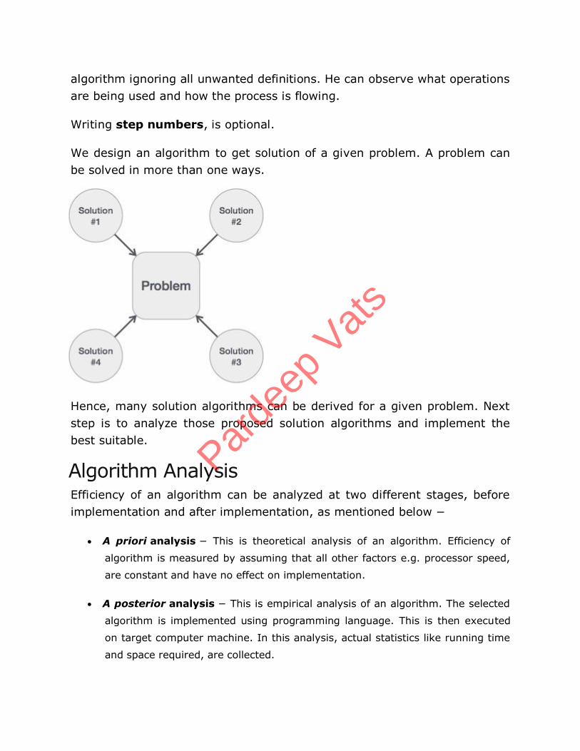
We design an algorithm to get solution of a given problem. A problem can
be solved in more than one ways.
Hence, many solution algorithms can be derived for a given problem. Next
step is to analyze those proposed solution algorithms and implement the
best suitable.
Algorithm Analysis Efficiency of an algorithm can be analyzed at two different stages, before
implementation and after implementation, as mentioned below −
A priori analysis − This is theoretical analysis of an algorithm. Efficiency of
algorithm is measured by assuming that all other factors e.g. processor speed,
are constant and have no effect on implementation.
A posterior analysis − This is empirical analysis of an algorithm. The selected
algorithm is implemented using programming language. This is then executed
on target computer machine. In this analysis, actual statistics like running time
and space required, are collected.
Parde
ep V
ats
We shall learn here a priori algorithm analysis. Algorithm analysis deals
with the execution or running time of various operations involved. Running
time of an operation can be defined as no. of computer instructions
executed per operation.
Algorithm Complexity Suppose X is an algorithm and n is the size of input data, the time and
space used by the Algorithm X are the two main factors which decide the
efficiency of X.
Time Factor − The time is measured by counting the number of key operations
such as comparisons in sorting algorithm
Space Factor − The space is measured by counting the maximum memory
space required by the algorithm.
The complexity of an algorithm f(n) gives the running time and / or storage
space required by the algorithm in terms of n as the size of input data.
Space Complexity Space complexity of an algorithm represents the amount of memory space
required by the algorithm in its life cycle. Space required by an algorithm is
equal to the sum of the following two components −
A fixed part that is a space required to store certain data and variables, that are
independent of the size of the problem. For example simple variables & constant
used, program size etc.
A variable part is a space required by variables, whose size depends on the size
of the problem. For example dynamic memory allocation, recursion stack space
etc.
Space complexity S(P) of any algorithm P is S(P) = C + SP(I) Where C is the
fixed part and S(I) is the variable part of the algorithm which depends on
instance characteristic I. Following is a simple example that tries to explain
the concept −
Parde
ep V
ats
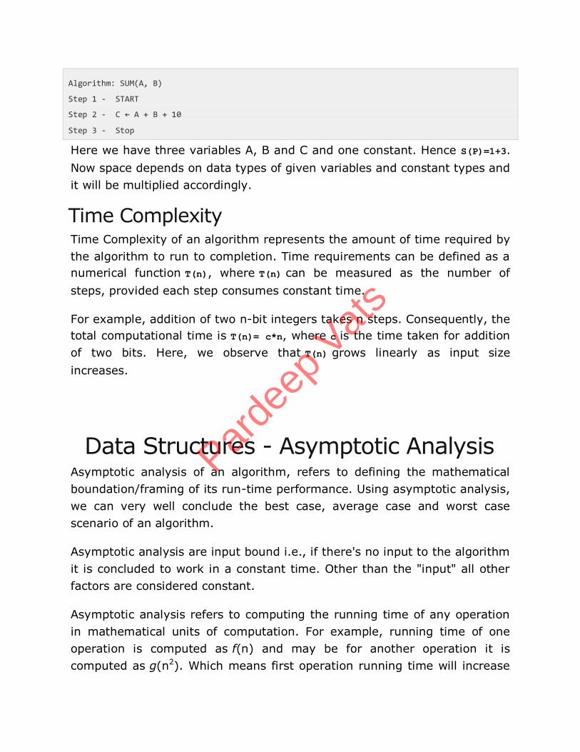
Algorithm: SUM(A, B)
Step 1 - START
Step 2 - C ← A + B + 10
Step 3 - Stop
Here we have three variables A, B and C and one constant. Hence S(P)=1+3.
Now space depends on data types of given variables and constant types and
it will be multiplied accordingly.
Time Complexity Time Complexity of an algorithm represents the amount of time required by
the algorithm to run to completion. Time requirements can be defined as a
numerical function T(n), where T(n) can be measured as the number of
steps, provided each step consumes constant time.
For example, addition of two n-bit integers takes n steps. Consequently, the
total computational time is T(n)= c*n, where c is the time taken for addition
of two bits. Here, we observe that T(n) grows linearly as input size
increases.
Data Structures - Asymptotic Analysis Asymptotic analysis of an algorithm, refers to defining the mathematical
boundation/framing of its run-time performance. Using asymptotic analysis,
we can very well conclude the best case, average case and worst case
scenario of an algorithm.
Asymptotic analysis are input bound i.e., if there's no input to the algorithm
it is concluded to work in a constant time. Other than the "input" all other
factors are considered constant.
Asymptotic analysis refers to computing the running time of any operation
in mathematical units of computation. For example, running time of one
operation is computed as f(n) and may be for another operation it is
computed as g(n2). Which means first operation running time will increase
Parde
ep V
ats
linearly with the increase in n and running time of second operation will
increase exponentially when n increases. Similarly the running time of both
operations will be nearly same if n is significantly small.
Usually, time required by an algorithm falls under three types −
Best Case − Minimum time required for program execution.
Average Case − Average time required for program execution.
Worst Case − Maximum time required for program execution.
Asymptotic Notations Following are commonly used asymptotic notations used in calculating
running time complexity of an algorithm.
Ο Notation
Ω Notation
θ Notation
Big Oh Notation, Ο
The Ο(n) is the formal way to express the upper bound of an algorithm's
running time. It measures the worst case time complexity or longest
amount of time an algorithm can possibly take to complete. For example,
for a functionf(n)
Ο(f(n)) = { g(n) : there exists c > 0 and n0 such that g(n) ≤ c.f(n) for all n > n0. }
Omega Notation, Ω
The Ω(n) is the formal way to express the lower bound of an algorithm's
running time. It measures the best case time complexity or best amount of
time an algorithm can possibly take to complete.
For example, for a function f(n)
Ω(f(n)) ≥ { g(n) : there exists c > 0 and n0 such that g(n) ≤ c.f(n) for all n > n0. }
Parde
ep V
ats
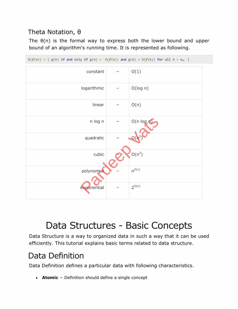
Theta Notation, θ
The θ(n) is the formal way to express both the lower bound and upper
bound of an algorithm's running time. It is represented as following.
θ(f(n)) = { g(n) if and only if g(n) = Ο(f(n)) and g(n) = Ω(f(n)) for all n > n0. }
constant − Ο(1)
logarithmic − Ο(log n)
linear − Ο(n)
n log n − Ο(n log n)
quadratic − Ο(n2)
cubic − Ο(n3)
polynomial − nΟ(1)
exponential − 2Ο(n)
Data Structures - Basic Concepts Data Structure is a way to organized data in such a way that it can be used
efficiently. This tutorial explains basic terms related to data structure.
Data Definition Data Definition defines a particular data with following characteristics.
Atomic − Definition should define a single concept
Parde
ep V
ats
Traceable − Definition should be be able to be mapped to some data element.
Accurate − Definition should be unambiguous.
Clear and Concise − Definition should be understandable.
Data Object Data Object represents an object having a data.
Data Type Data type is way to classify various types of data such as integer, string etc.
which determines the values that can be used with the corresponding type
of data, the type of operations that can be performed on the corresponding
type of data. Data type of two types −
Built-in Data Type
Derived Data Type
Built-in Data Type
Those data types for which a language has built-in support are known as
Built-in Data types. For example, most of the languages provides following
built-in data types.
Integers
Boolean (true, false)
Floating (Decimal numbers)
Character and Strings
Derived Data Type
Those data types which are implementation independent as they can be
implemented in one or other way are known as derived data types. These
Parde
ep V
ats
data types are normally built by combination of primary or built-in data
types and associated operations on them. For example −
List
Array
Stack
Queue
Basic Operations The data in the data structures are processed by certain operations. The
particular data structure chosen largely depends on the frequency of the
operation that needs to be performed on the data structure.
Traversing
Searching
Insertion
Deletion
Sorting
Merging
Data Structure - Arrays Array Basics Array is a container which can hold fix number of items and these items
should be of same type. Most of the datastructure make use of array to
implement their algorithms. Following are important terms to understand
the concepts of Array.
Element − Each item stored in an array is called an element.
Index − Each location of an element in an array has a numerical index which is
used to identify the element.
Parde
ep V
ats
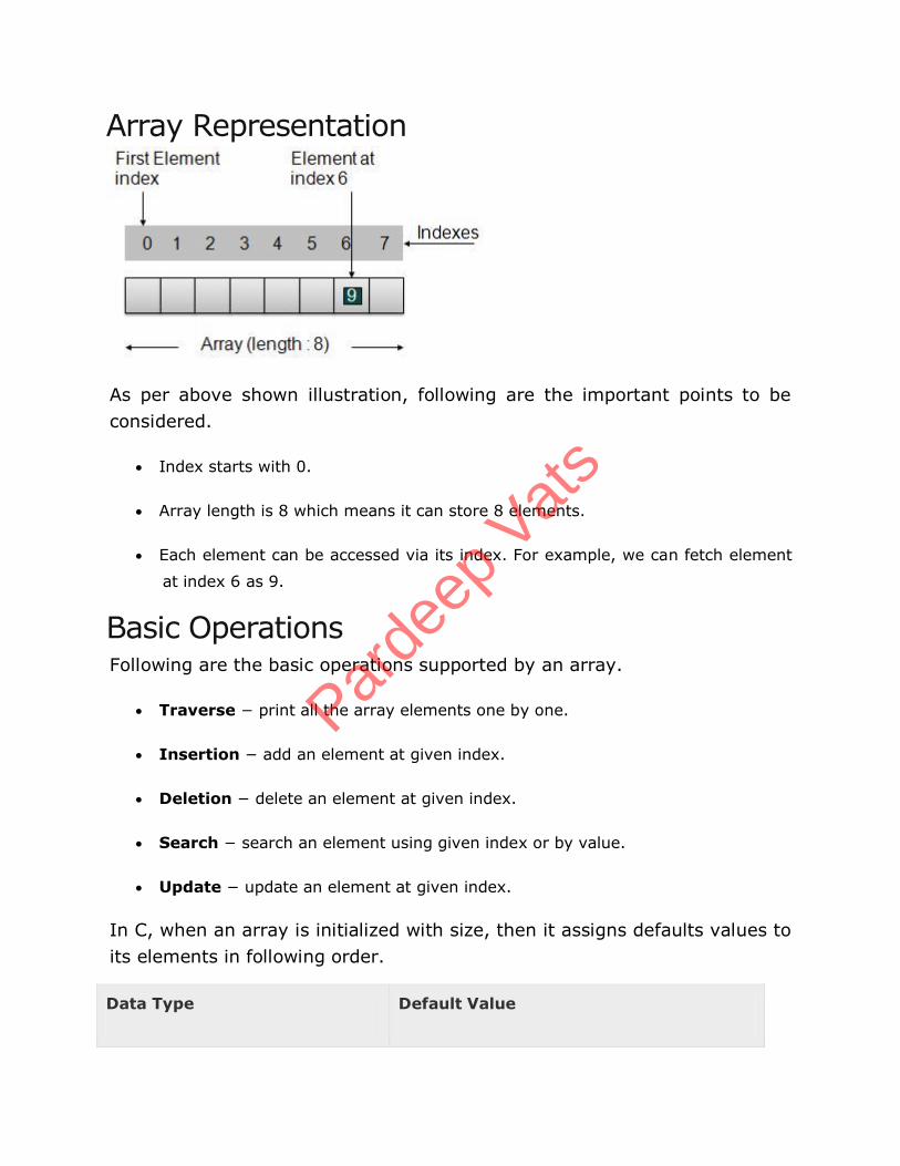
Array Representation
As per above shown illustration, following are the important points to be
considered.
Index starts with 0.
Array length is 8 which means it can store 8 elements.
Each element can be accessed via its index. For example, we can fetch element
at index 6 as 9.
Basic Operations Following are the basic operations supported by an array.
Traverse − print all the array elements one by one.
Insertion − add an element at given index.
Deletion − delete an element at given index.
Search − search an element using given index or by value.
Update − update an element at given index.
In C, when an array is initialized with size, then it assigns defaults values to
its elements in following order.
Data Type Default Value
Parde
ep V
ats
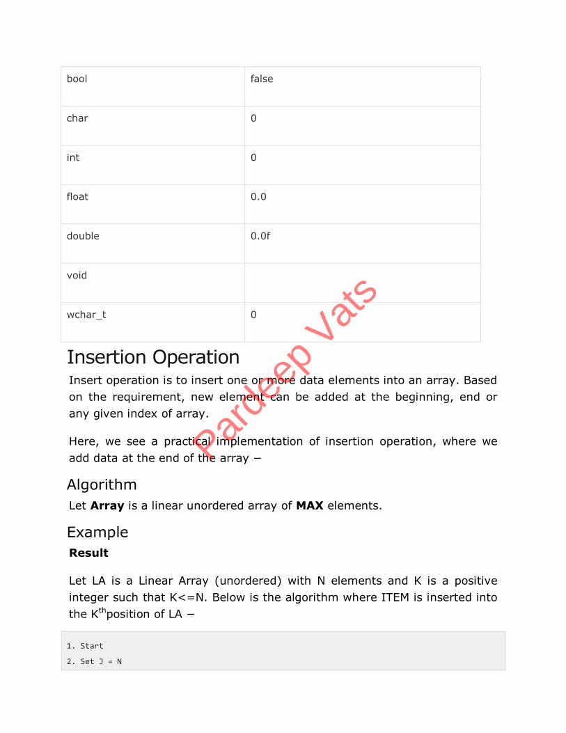
bool false
char 0
int 0
float 0.0
double 0.0f
void
wchar_t 0
Insertion Operation Insert operation is to insert one or more data elements into an array. Based
on the requirement, new element can be added at the beginning, end or
any given index of array.
Here, we see a practical implementation of insertion operation, where we
add data at the end of the array −
Algorithm
Let Array is a linear unordered array of MAX elements.
Example
Result
Let LA is a Linear Array (unordered) with N elements and K is a positive
integer such that K<=N. Below is the algorithm where ITEM is inserted into
the Kthposition of LA −
1. Start
2. Set J = N
Parde
ep V
ats
3. Set N = N+1
4. Repeat steps 5 and 6 while J >= K
5. Set LA[J+1] = LA[J]
6. Set J = J-1
7. Set LA[K] = ITEM
8. Stop
Example
Below is the implementation of the above algorithm −
#include <stdio.h>
main() {
int LA[] = {1,3,5,7,8};
int item = 10, k = 3, n = 5;
int i = 0, j = n;
printf("The original array elements are :\n");
for(i = 0; i<n; i++) {
printf("LA[%d] = %d \n", i, LA[i]);
}
n = n + 1;
while( j >= k){
LA[j+1] = LA[j];
j = j - 1;
}
LA[k] = item;
printf("The array elements after insertion :\n");
for(i = 0; i<n; i++) {
printf("LA[%d] = %d \n", i, LA[i]);
Parde
ep V
ats
}
}
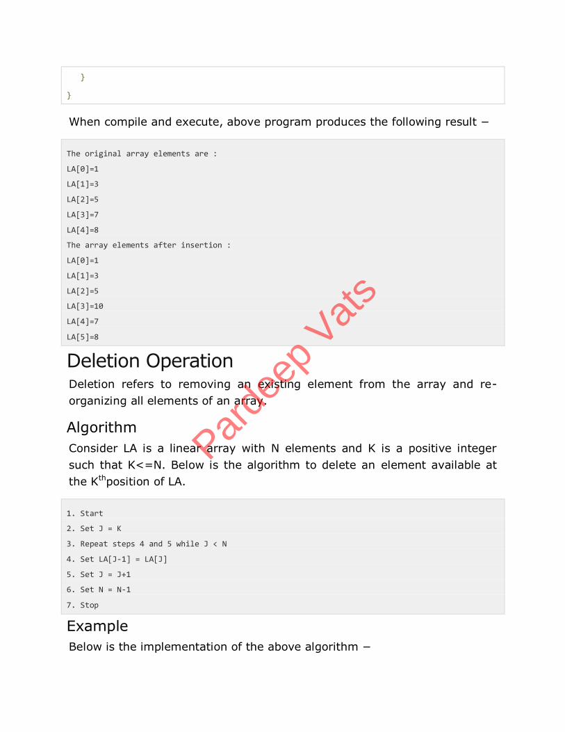
When compile and execute, above program produces the following result −
The original array elements are :
LA[0]=1
LA[1]=3
LA[2]=5
LA[3]=7
LA[4]=8
The array elements after insertion :
LA[0]=1
LA[1]=3
LA[2]=5
LA[3]=10
LA[4]=7
LA[5]=8
Deletion Operation Deletion refers to removing an existing element from the array and re-
organizing all elements of an array.
Algorithm
Consider LA is a linear array with N elements and K is a positive integer
such that K<=N. Below is the algorithm to delete an element available at
the Kthposition of LA.
1. Start
2. Set J = K
3. Repeat steps 4 and 5 while J < N
4. Set LA[J-1] = LA[J]
5. Set J = J+1
6. Set N = N-1
7. Stop
Example
Below is the implementation of the above algorithm −
Parde
ep V
ats
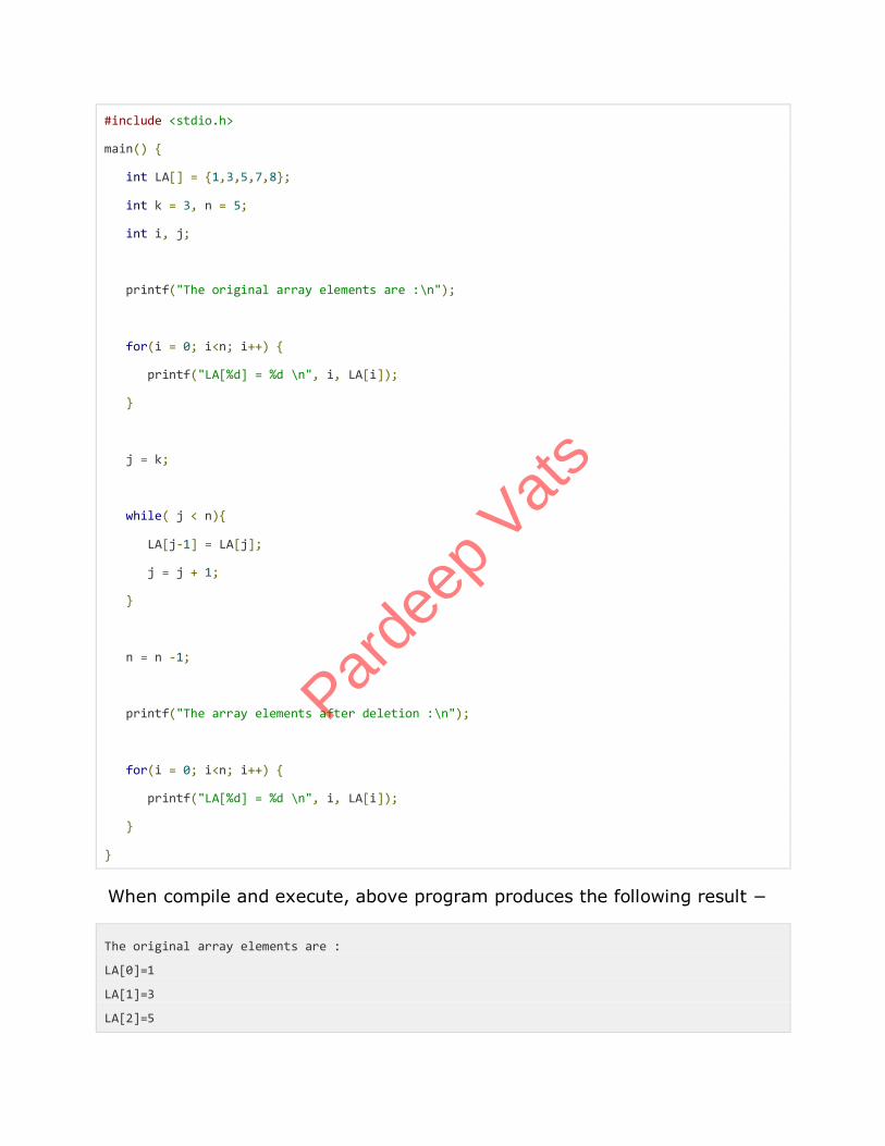
#include <stdio.h>
main() {
int LA[] = {1,3,5,7,8};
int k = 3, n = 5;
int i, j;
printf("The original array elements are :\n");
for(i = 0; i<n; i++) {
printf("LA[%d] = %d \n", i, LA[i]);
}
j = k;
while( j < n){
LA[j-1] = LA[j];
j = j + 1;
}
n = n -1;
printf("The array elements after deletion :\n");
for(i = 0; i<n; i++) {
printf("LA[%d] = %d \n", i, LA[i]);
}
}
When compile and execute, above program produces the following result −
The original array elements are :
LA[0]=1
LA[1]=3
LA[2]=5
Parde
ep V
ats

LA[3]=7
LA[4]=8
The array elements after deletion :
LA[0]=1
LA[1]=3
LA[2]=7
LA[3]=8
Search Operation You can perform a search for array element based on its value or its index.
Algorithm
Consider LA is a linear array with N elements and K is a positive integer
such that K<=N. Below is the algorithm to find an element with a value of
ITEM using sequential search.
1. Start
2. Set J = 0
3. Repeat steps 4 and 5 while J < N
4. IF LA[J] is equal ITEM THEN GOTO STEP 6
5. Set J = J +1
6. PRINT J, ITEM
7. Stop
Example
Below is the implementation of the above algorithm −
#include <stdio.h>
main() {
int LA[] = {1,3,5,7,8};
int item = 5, n = 5;
int i = 0, j = 0;
printf("The original array elements are :\n");
for(i = 0; i<n; i++) {
printf("LA[%d] = %d \n", i, LA[i]);
Parde
ep V
ats
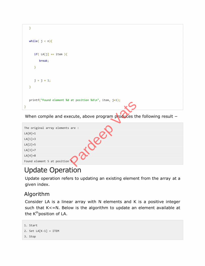
}
while( j < n){
if( LA[j] == item ){
break;
}
j = j + 1;
}
printf("Found element %d at position %d\n", item, j+1);
}
When compile and execute, above program produces the following result −
The original array elements are :
LA[0]=1
LA[1]=3
LA[2]=5
LA[3]=7
LA[4]=8
Found element 5 at position 3
Update Operation Update operation refers to updating an existing element from the array at a
given index.
Algorithm
Consider LA is a linear array with N elements and K is a positive integer
such that K<=N. Below is the algorithm to update an element available at
the Kthposition of LA.
1. Start
2. Set LA[K-1] = ITEM
3. Stop
Parde
ep V
ats
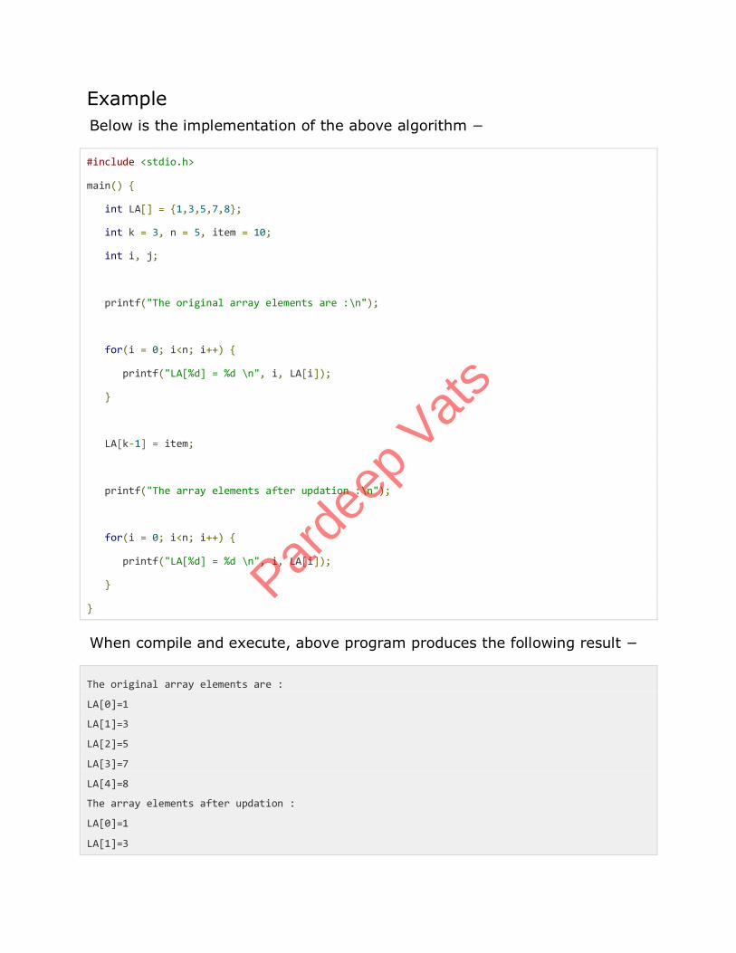
Example
Below is the implementation of the above algorithm −
#include <stdio.h>
main() {
int LA[] = {1,3,5,7,8};
int k = 3, n = 5, item = 10;
int i, j;
printf("The original array elements are :\n");
for(i = 0; i<n; i++) {
printf("LA[%d] = %d \n", i, LA[i]);
}
LA[k-1] = item;
printf("The array elements after updation :\n");
for(i = 0; i<n; i++) {
printf("LA[%d] = %d \n", i, LA[i]);
}
}
When compile and execute, above program produces the following result −
The original array elements are :
LA[0]=1
LA[1]=3
LA[2]=5
LA[3]=7
LA[4]=8
The array elements after updation :
LA[0]=1
LA[1]=3
Parde
ep V
ats
LA[2]=10
LA[3]=7
LA[4]=8
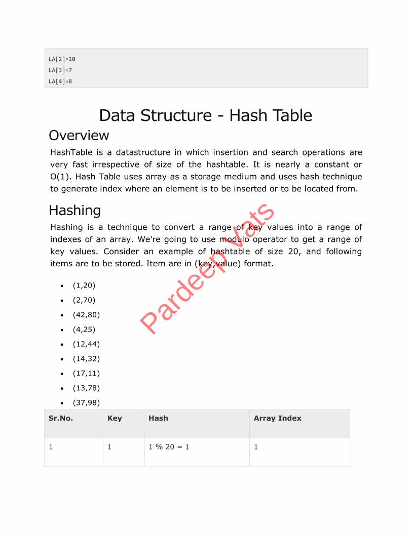
Data Structure - Hash Table Overview HashTable is a datastructure in which insertion and search operations are
very fast irrespective of size of the hashtable. It is nearly a constant or
O(1). Hash Table uses array as a storage medium and uses hash technique
to generate index where an element is to be inserted or to be located from.
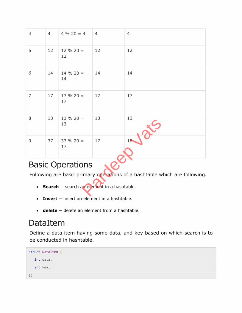
Hashing Hashing is a technique to convert a range of key values into a range of
indexes of an array. We're going to use modulo operator to get a range of
key values. Consider an example of hashtable of size 20, and following
items are to be stored. Item are in (key,value) format.
(1,20)
(2,70)
(42,80)
(4,25)
(12,44)
(14,32)
(17,11)
(13,78)
(37,98)
Sr.No. Key Hash Array Index
1 1 1 % 20 = 1 1
Parde
ep V
ats
2 2 2 % 20 = 2 2
3 42 42 % 20 = 2 2
4 4 4 % 20 = 4 4
5 12 12 % 20 = 12 12
6 14 14 % 20 = 14 14
7 17 17 % 20 = 17 17
8 13 13 % 20 = 13 13
9 37 37 % 20 = 17 17
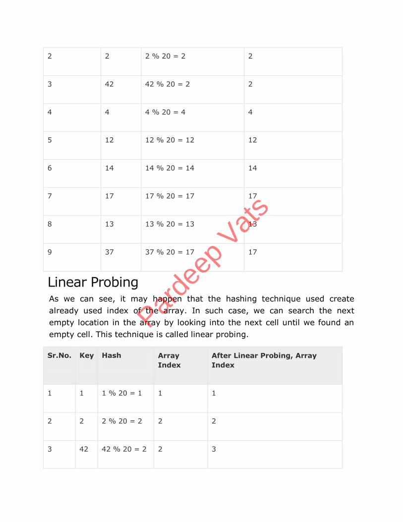
Linear Probing As we can see, it may happen that the hashing technique used create
already used index of the array. In such case, we can search the next
empty location in the array by looking into the next cell until we found an
empty cell. This technique is called linear probing.
Sr.No. Key Hash Array
Index
After Linear Probing, Array
Index
1 1 1 % 20 = 1 1 1
2 2 2 % 20 = 2 2 2
3 42 42 % 20 = 2 2 3
Parde
ep V
ats
4 4 4 % 20 = 4 4 4
5 12 12 % 20 =
12
12 12
6 14 14 % 20 =
14
14 14
7 17 17 % 20 =
17
17 17
8 13 13 % 20 =
13
13 13
9 37 37 % 20 =
17
17 18
Basic Operations Following are basic primary operations of a hashtable which are following.
Search − search an element in a hashtable.
Insert − insert an element in a hashtable.
delete − delete an element from a hashtable.
DataItem Define a data item having some data, and key based on which search is to
be conducted in hashtable.
struct DataItem {
int data;
int key;
};
Parde
ep V
ats
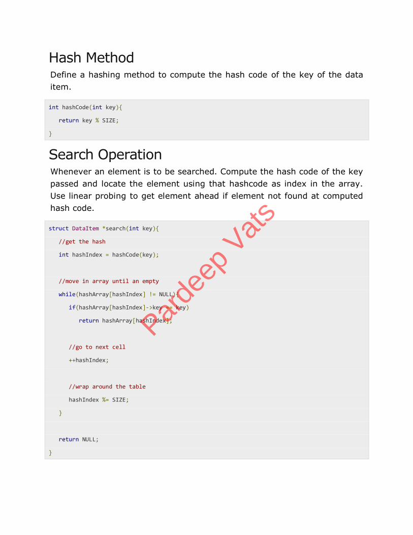
Hash Method Define a hashing method to compute the hash code of the key of the data
item.
int hashCode(int key){
return key % SIZE;
}
Search Operation Whenever an element is to be searched. Compute the hash code of the key
passed and locate the element using that hashcode as index in the array.
Use linear probing to get element ahead if element not found at computed
hash code.
struct DataItem *search(int key){
//get the hash
int hashIndex = hashCode(key);
//move in array until an empty
while(hashArray[hashIndex] != NULL){
if(hashArray[hashIndex]->key == key)
return hashArray[hashIndex];
//go to next cell
++hashIndex;
//wrap around the table
hashIndex %= SIZE;
}
return NULL;
}
Parde
ep V
ats
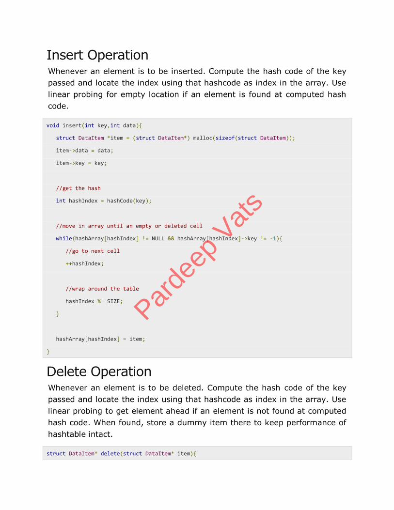
Insert Operation Whenever an element is to be inserted. Compute the hash code of the key
passed and locate the index using that hashcode as index in the array. Use
linear probing for empty location if an element is found at computed hash
code.
void insert(int key,int data){
struct DataItem *item = (struct DataItem*) malloc(sizeof(struct DataItem));
item->data = data;
item->key = key;
//get the hash
int hashIndex = hashCode(key);
//move in array until an empty or deleted cell
while(hashArray[hashIndex] != NULL && hashArray[hashIndex]->key != -1){
//go to next cell
++hashIndex;
//wrap around the table
hashIndex %= SIZE;
}
hashArray[hashIndex] = item;
}
Delete Operation Whenever an element is to be deleted. Compute the hash code of the key
passed and locate the index using that hashcode as index in the array. Use
linear probing to get element ahead if an element is not found at computed
hash code. When found, store a dummy item there to keep performance of
hashtable intact.
struct DataItem* delete(struct DataItem* item){
Parde
ep V
ats
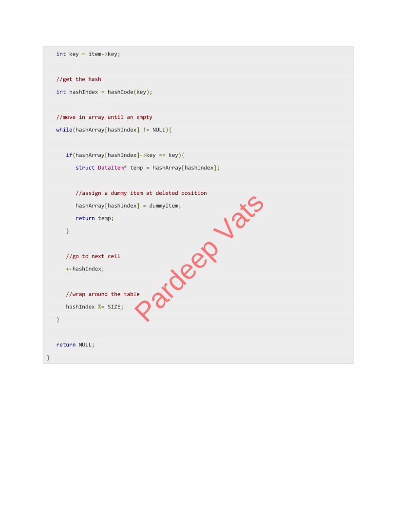
int key = item->key;
//get the hash
int hashIndex = hashCode(key);
//move in array until an empty
while(hashArray[hashIndex] != NULL){
if(hashArray[hashIndex]->key == key){
struct DataItem* temp = hashArray[hashIndex];
//assign a dummy item at deleted position
hashArray[hashIndex] = dummyItem;
return temp;
}
//go to next cell
++hashIndex;
//wrap around the table
hashIndex %= SIZE;
}
return NULL;
}
Parde
ep V
ats
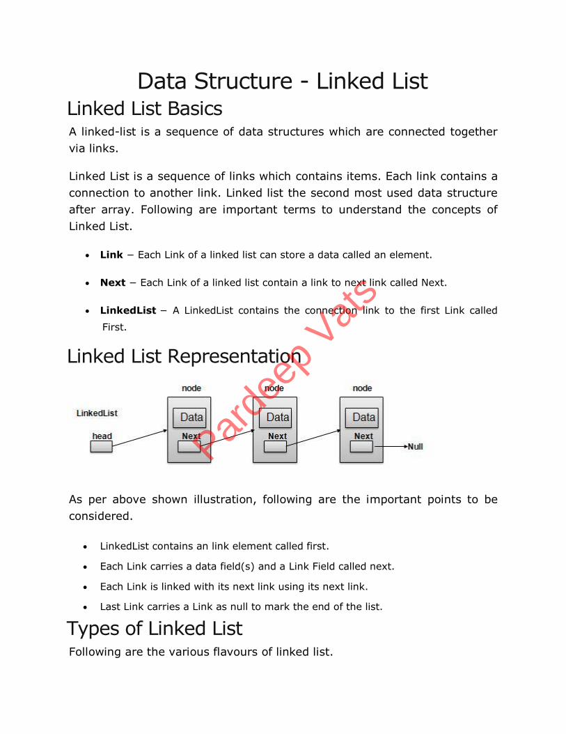
Data Structure - Linked List Linked List Basics A linked-list is a sequence of data structures which are connected together
via links.
Linked List is a sequence of links which contains items. Each link contains a
connection to another link. Linked list the second most used data structure
after array. Following are important terms to understand the concepts of
Linked List.
Link − Each Link of a linked list can store a data called an element.
Next − Each Link of a linked list contain a link to next link called Next.
LinkedList − A LinkedList contains the connection link to the first Link called
First.
Linked List Representation
As per above shown illustration, following are the important points to be
considered.
LinkedList contains an link element called first.
Each Link carries a data field(s) and a Link Field called next.
Each Link is linked with its next link using its next link.
Last Link carries a Link as null to mark the end of the list.
Types of Linked List Following are the various flavours of linked list.
Parde
ep V
ats
Simple Linked List − Item Navigation is forward only.
Doubly Linked List − Items can be navigated forward and backward way.
Circular Linked List − Last item contains link of the first element as next and
and first element has link to last element as prev.
Basic Operations Following are the basic operations supported by a list.
Insertion − add an element at the beginning of the list.
Deletion − delete an element at the beginning of the list.
Display − displaying complete list.
Search − search an element using given key.
Delete − delete an element using given key.
Insertion Operation Insertion is a three step process −
Create a new Link with provided data.
Point New Link to old First Link.
Point First Link to this New Link. Par
deep
Vat
s
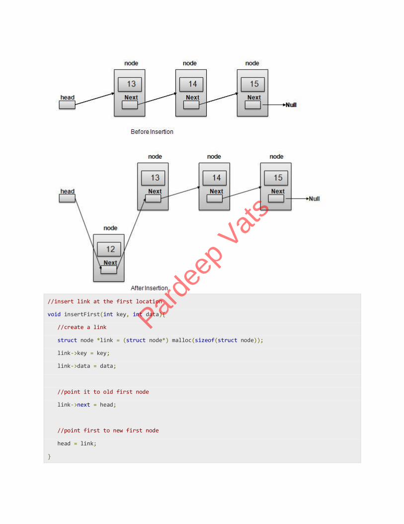
//insert link at the first location
void insertFirst(int key, int data){
//create a link
struct node *link = (struct node*) malloc(sizeof(struct node));
link->key = key;
link->data = data;
//point it to old first node
link->next = head;
//point first to new first node
head = link;
}
Parde
ep V
ats
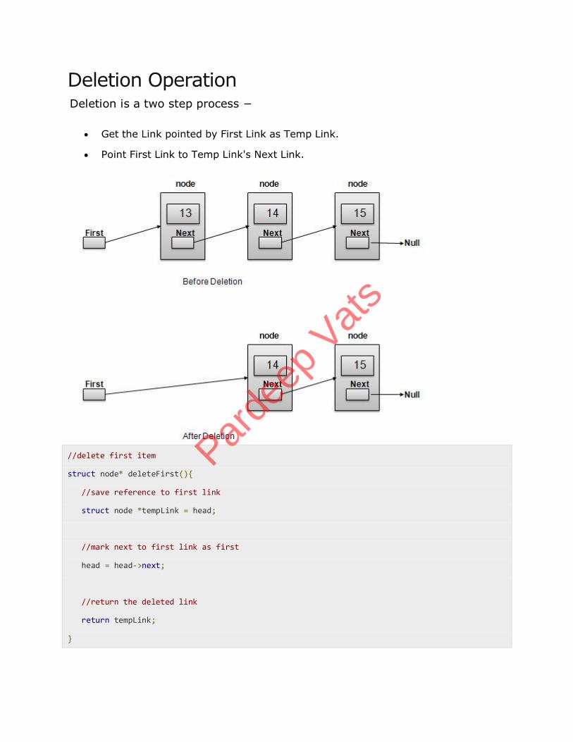
Deletion Operation Deletion is a two step process −
Get the Link pointed by First Link as Temp Link.
Point First Link to Temp Link's Next Link.
//delete first item
struct node* deleteFirst(){
//save reference to first link
struct node *tempLink = head;
//mark next to first link as first
head = head->next;
//return the deleted link
return tempLink;
}
Parde
ep V
ats
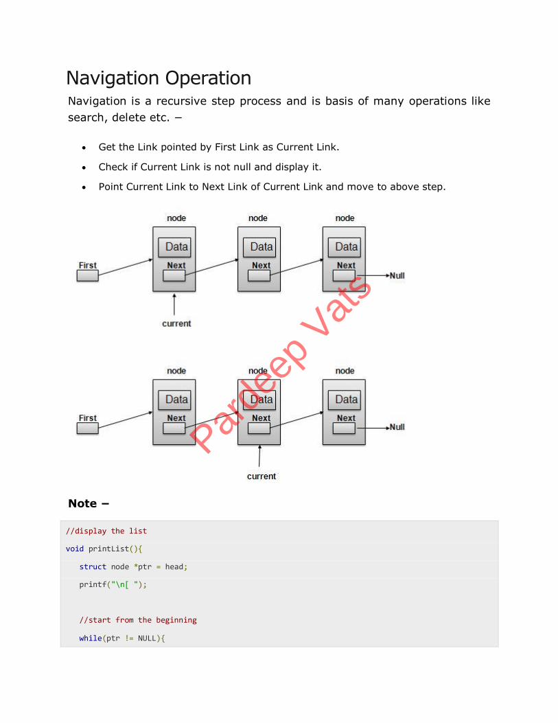
Navigation Operation Navigation is a recursive step process and is basis of many operations like
search, delete etc. −
Get the Link pointed by First Link as Current Link.
Check if Current Link is not null and display it.
Point Current Link to Next Link of Current Link and move to above step.
Note −
//display the list
void printList(){
struct node *ptr = head;
printf("\n[ ");
//start from the beginning
while(ptr != NULL){
Parde
ep V
ats
printf("(%d,%d) ",ptr->key,ptr->data);
ptr = ptr->next;
}
printf(" ]");
}
Advanced Operations Following are the advanced operations specified for a list.
Sort − sorting a list based on a particular order.
Reverse − reversing a linked list.
Sort Operation We've used bubble sort to sort a list.
void sort(){
int i, j, k, tempKey, tempData ;
struct node *current;
struct node *next;
int size = length();
k = size ;
for ( i = 0 ; i < size - 1 ; i++, k-- ) {
current = head ;
next = head->next ;
for ( j = 1 ; j < k ; j++ ) {
if ( current->data > next->data ) {
tempData = current->data ;
current->data = next->data;
Parde
ep V
ats
next->data = tempData ;
tempKey = current->key;
current->key = next->key;
next->key = tempKey;
}
current = current->next;
next = next->next;
}
}
}
Reverse Operation Following code demonstrate reversing a single linked list.
void reverse(struct node** head_ref) {
struct node* prev = NULL;
struct node* current = *head_ref;
struct node* next;
while (current != NULL) {
next = current->next;
current->next = prev;
prev = current;
current = next;
}
*head_ref = prev;
}
Parde
ep V
ats
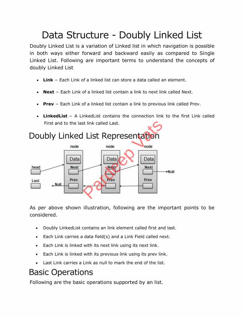
Data Structure - Doubly Linked List Doubly Linked List is a variation of Linked list in which navigation is possible
in both ways either forward and backward easily as compared to Single
Linked List. Following are important terms to understand the concepts of
doubly Linked List
Link − Each Link of a linked list can store a data called an element.
Next − Each Link of a linked list contain a link to next link called Next.
Prev − Each Link of a linked list contain a link to previous link called Prev.
LinkedList − A LinkedList contains the connection link to the first Link called
First and to the last link called Last.
Doubly Linked List Representation
As per above shown illustration, following are the important points to be
considered.
Doubly LinkedList contains an link element called first and last.
Each Link carries a data field(s) and a Link Field called next.
Each Link is linked with its next link using its next link.
Each Link is linked with its previous link using its prev link.
Last Link carries a Link as null to mark the end of the list.
Basic Operations Following are the basic operations supported by an list.
Parde
ep V
ats
Insertion − add an element at the beginning of the list.
Deletion − delete an element at the beginning of the list.
Insert Last − add an element in the end of the list.
Delete Last − delete an element from the end of the list.
Insert After − add an element after an item of the list.
Delete − delete an element from the list using key.
Display forward − displaying complete list in forward manner.
Display backward − displaying complete list in backward manner.
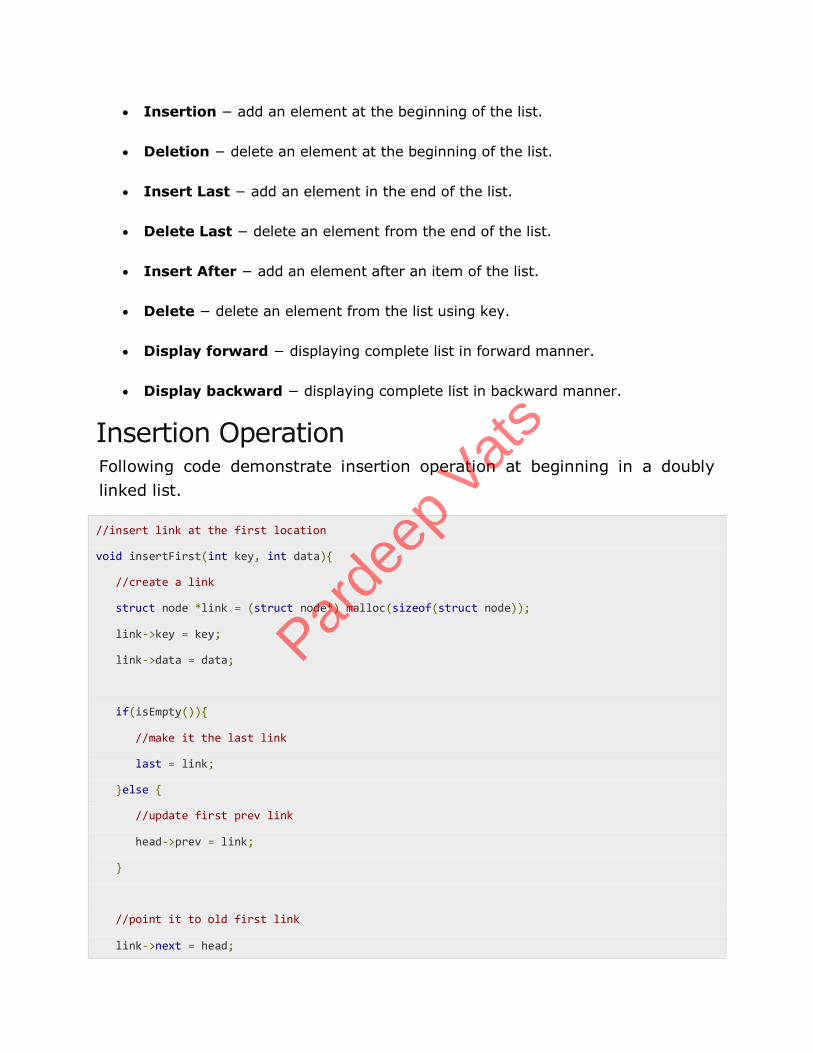
Insertion Operation Following code demonstrate insertion operation at beginning in a doubly
linked list.
//insert link at the first location
void insertFirst(int key, int data){
//create a link
struct node *link = (struct node*) malloc(sizeof(struct node));
link->key = key;
link->data = data;
if(isEmpty()){
//make it the last link
last = link;
}else {
//update first prev link
head->prev = link;
}
//point it to old first link
link->next = head;
Parde
ep V
ats
//point first to new first link
head = link;
}
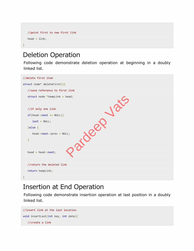
Deletion Operation Following code demonstrate deletion operation at beginning in a doubly
linked list.
//delete first item
struct node* deleteFirst(){
//save reference to first link
struct node *tempLink = head;
//if only one link
if(head->next == NULL){
last = NULL;
}else {
head->next->prev = NULL;
}
head = head->next;
//return the deleted link
return tempLink;
}
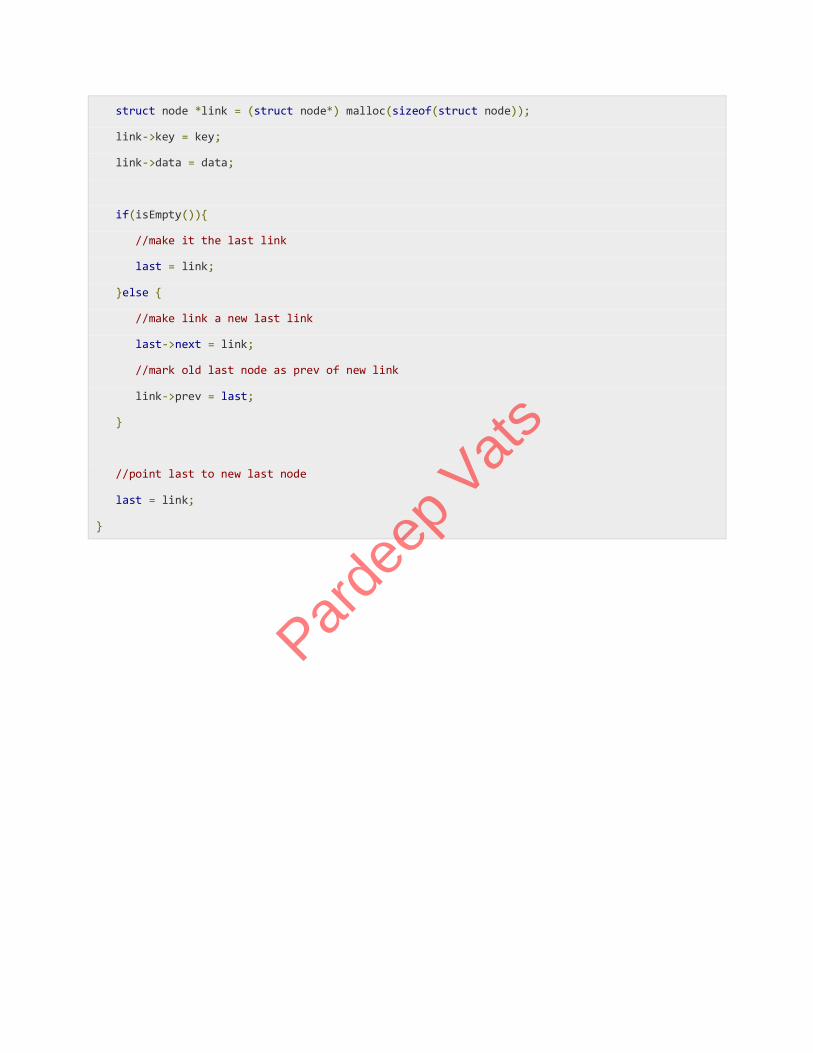
Insertion at End Operation Following code demonstrate insertion operation at last position in a doubly
linked list.
//insert link at the last location
void insertLast(int key, int data){
//create a link
Parde
ep V
ats
struct node *link = (struct node*) malloc(sizeof(struct node));
link->key = key;
link->data = data;
if(isEmpty()){
//make it the last link
last = link;
}else {
//make link a new last link
last->next = link;
//mark old last node as prev of new link
link->prev = last;
}
//point last to new last node
last = link;
}
Parde
ep V
ats
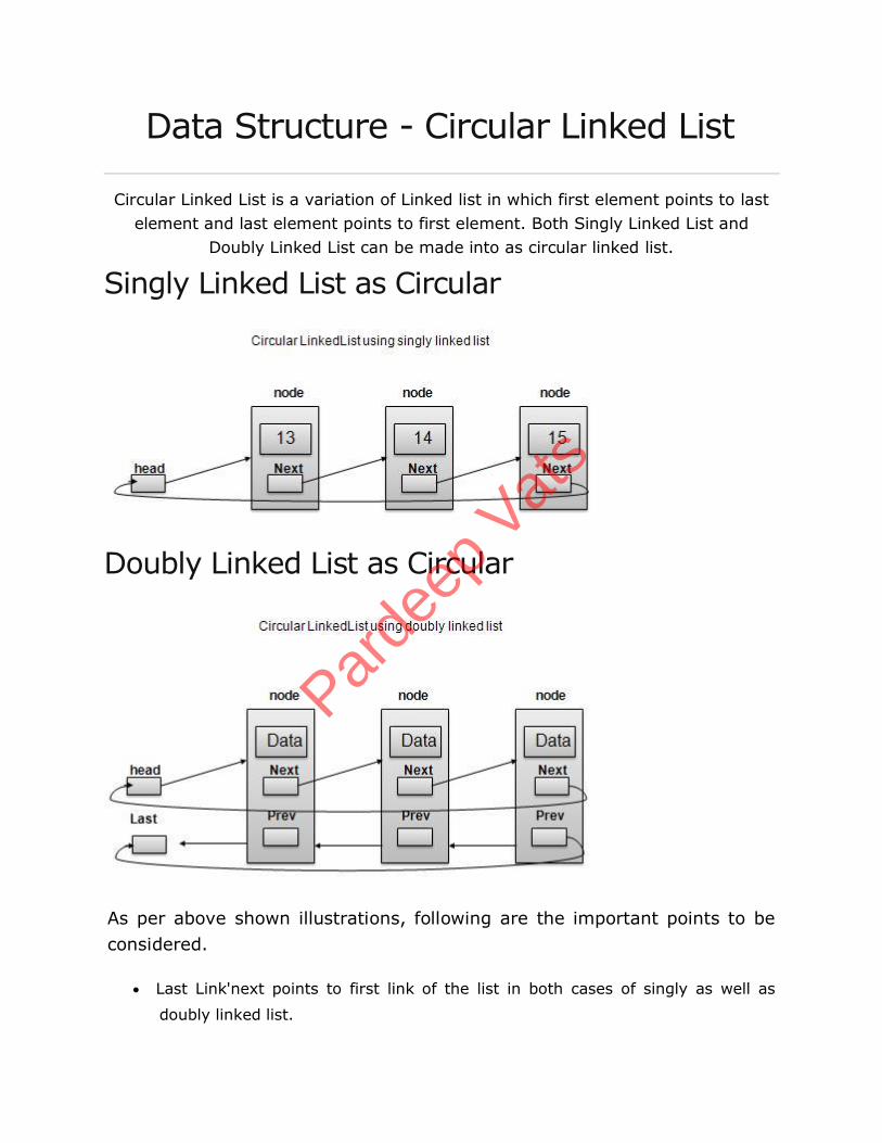
Data Structure - Circular Linked List
Circular Linked List is a variation of Linked list in which first element points to last
element and last element points to first element. Both Singly Linked List and
Doubly Linked List can be made into as circular linked list.
Singly Linked List as Circular
Doubly Linked List as Circular
As per above shown illustrations, following are the important points to be
considered.
Last Link'next points to first link of the list in both cases of singly as well as
doubly linked list.
Parde
ep V
ats
First Link's prev points to the last of the list in case of doubly linked list.
Basic Operations Following are the important operations supported by a circular list.
insert − insert an element in the start of the list.
delete − insert an element from the start of the list.
display − display the list.
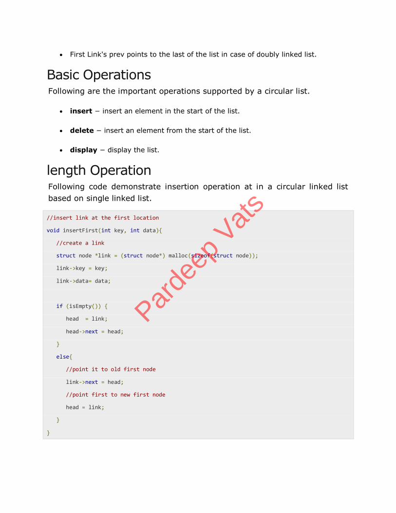
length Operation Following code demonstrate insertion operation at in a circular linked list
based on single linked list.
//insert link at the first location
void insertFirst(int key, int data){
//create a link
struct node *link = (struct node*) malloc(sizeof(struct node));
link->key = key;
link->data= data;
if (isEmpty()) {
head = link;
head->next = head;
}
else{
//point it to old first node
link->next = head;
//point first to new first node
head = link;
}
}
Parde
ep V
ats
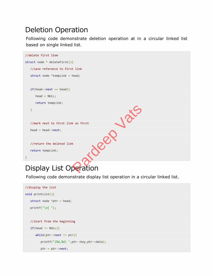
Deletion Operation Following code demonstrate deletion operation at in a circular linked list
based on single linked list.
//delete first item
struct node * deleteFirst(){
//save reference to first link
struct node *tempLink = head;
if(head->next == head){
head = NULL;
return tempLink;
}
//mark next to first link as first
head = head->next;
//return the deleted link
return tempLink;
}
Display List Operation Following code demonstrate display list operation in a circular linked list.
//display the list
void printList(){
struct node *ptr = head;
printf("\n[ ");
//start from the beginning
if(head != NULL){
while(ptr->next != ptr){
printf("(%d,%d) ",ptr->key,ptr->data);
ptr = ptr->next;
Parde
ep V
ats
}
}
printf(" ]");
}
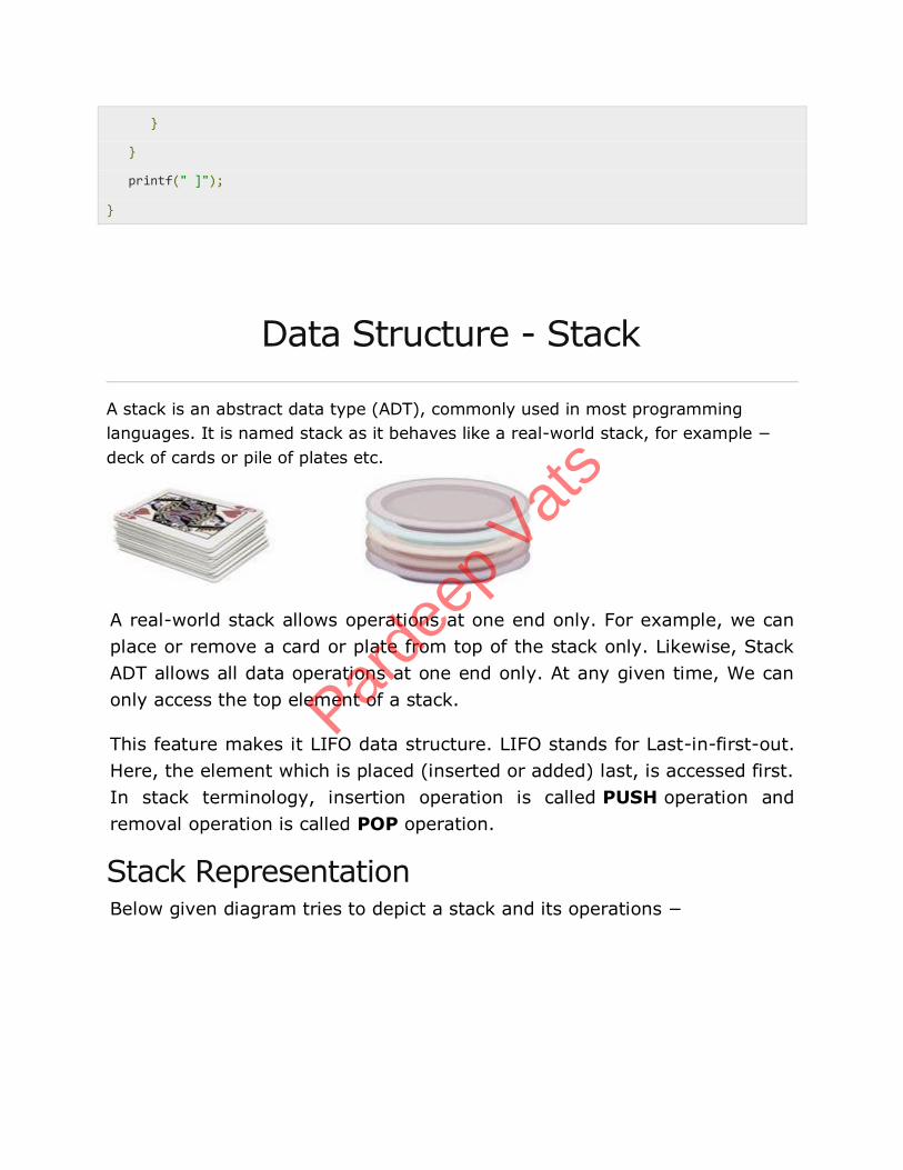
Data Structure - Stack
A stack is an abstract data type (ADT), commonly used in most programming
languages. It is named stack as it behaves like a real-world stack, for example −
deck of cards or pile of plates etc.
A real-world stack allows operations at one end only. For example, we can
place or remove a card or plate from top of the stack only. Likewise, Stack
ADT allows all data operations at one end only. At any given time, We can
only access the top element of a stack.
This feature makes it LIFO data structure. LIFO stands for Last-in-first-out.
Here, the element which is placed (inserted or added) last, is accessed first.
In stack terminology, insertion operation is called PUSH operation and
removal operation is called POP operation.
Stack Representation Below given diagram tries to depict a stack and its operations −
Parde
ep V
ats
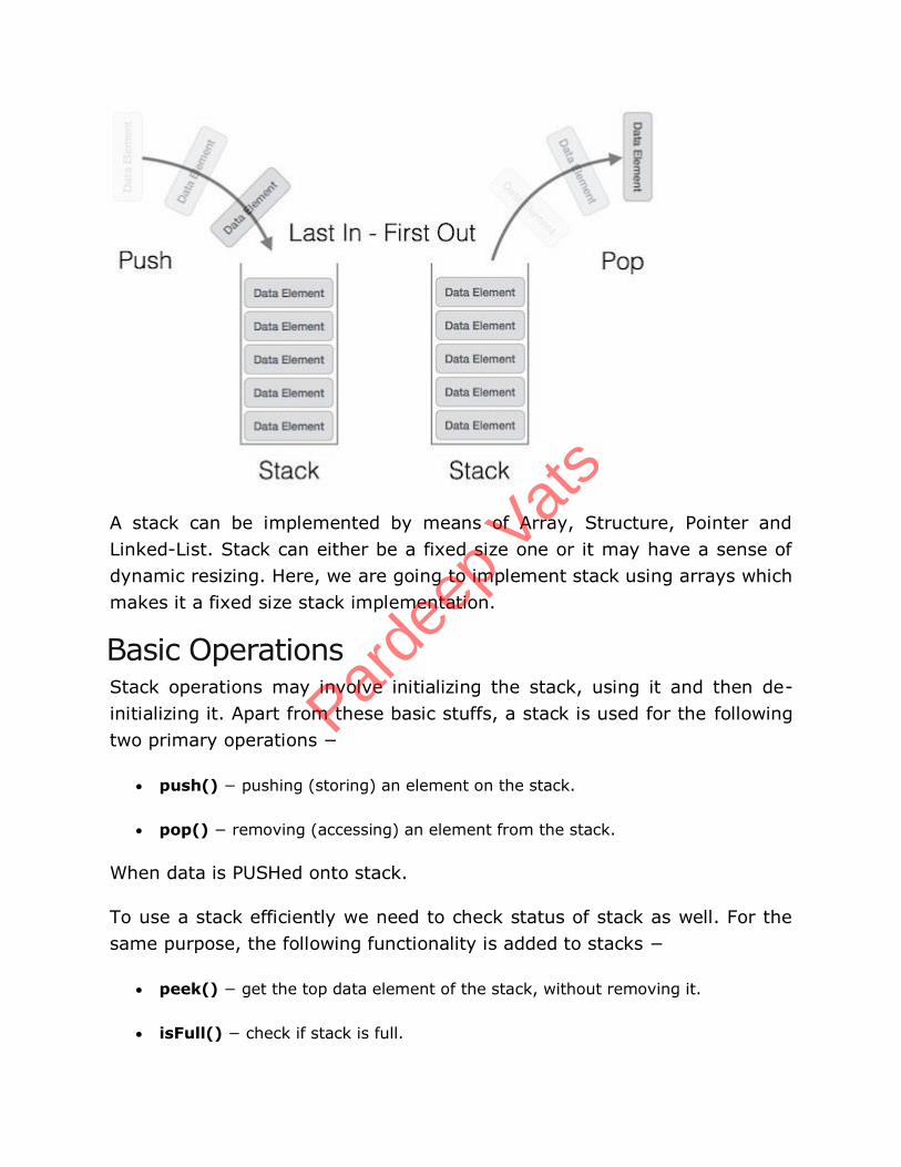
A stack can be implemented by means of Array, Structure, Pointer and
Linked-List. Stack can either be a fixed size one or it may have a sense of
dynamic resizing. Here, we are going to implement stack using arrays which
makes it a fixed size stack implementation.
Basic Operations Stack operations may involve initializing the stack, using it and then de-
initializing it. Apart from these basic stuffs, a stack is used for the following
two primary operations −
push() − pushing (storing) an element on the stack.
pop() − removing (accessing) an element from the stack.
When data is PUSHed onto stack.
To use a stack efficiently we need to check status of stack as well. For the
same purpose, the following functionality is added to stacks −
peek() − get the top data element of the stack, without removing it.
isFull() − check if stack is full.
Parde
ep V
ats
isEmpty() − check if stack is empty.
At all times, we maintain a pointer to the last PUSHed data on the stack. As
this pointer always represents the top of the stack, hence named top.
The toppointer provides top value of the stack without actually removing it.
First we should learn about procedures to support stack functions −
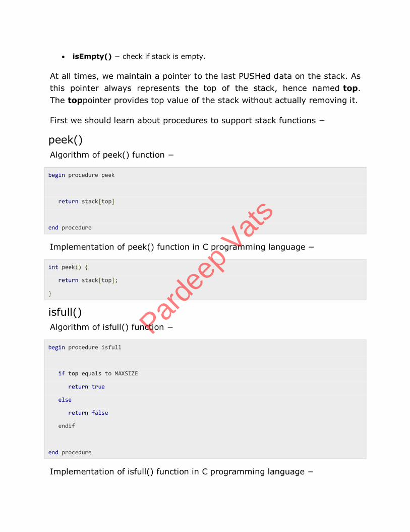
peek()
Algorithm of peek() function −
begin procedure peek
return stack[top]
end procedure
Implementation of peek() function in C programming language −
int peek() {
return stack[top];
}
isfull()
Algorithm of isfull() function −
begin procedure isfull
if top equals to MAXSIZE
return true
else
return false
endif
end procedure
Implementation of isfull() function in C programming language −
Parde
ep V
ats
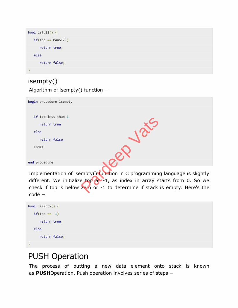
bool isfull() {
if(top == MAXSIZE)
return true;
else
return false;
}
isempty()
Algorithm of isempty() function −
begin procedure isempty
if top less than 1
return true
else
return false
endif
end procedure
Implementation of isempty() function in C programming language is slightly
different. We initialize top at -1, as index in array starts from 0. So we
check if top is below zero or -1 to determine if stack is empty. Here's the
code −
bool isempty() {
if(top == -1)
return true;
else
return false;
}
PUSH Operation The process of putting a new data element onto stack is known
as PUSHOperation. Push operation involves series of steps −
Parde
ep V
ats
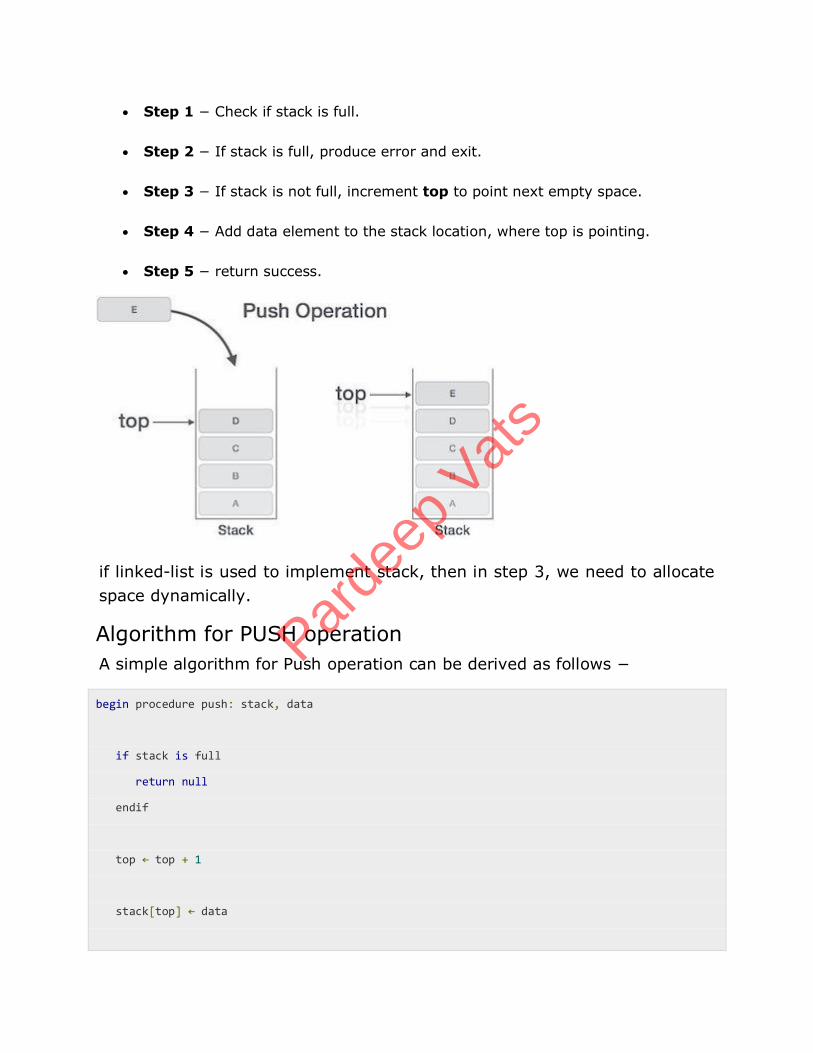
Step 1 − Check if stack is full.
Step 2 − If stack is full, produce error and exit.
Step 3 − If stack is not full, increment top to point next empty space.
Step 4 − Add data element to the stack location, where top is pointing.
Step 5 − return success.
if linked-list is used to implement stack, then in step 3, we need to allocate
space dynamically.
Algorithm for PUSH operation
A simple algorithm for Push operation can be derived as follows −
begin procedure push: stack, data
if stack is full
return null
endif
top ← top + 1
stack[top] ← data
Parde
ep V
ats
end procedure
Implementation of this algorithm in C, is very easy. See the below code −
void push(int data) {
if(!isFull()) {
top = top + 1;
stack[top] = data;
}
else {
printf("Could not insert data, Stack is full.\n");
}
}
Pop Operation Accessing the content while removing it from stack, is known as pop
operation. In array implementation of pop() operation, data element is not
actually removed, instead top is decremented to a lower position in stack to
point to next value. But in linked-list implementation, pop() actually
removes data element and deallocates memory space.
A POP operation may involve the following steps −
Step 1 − Check if stack is empty.
Step 2 − If stack is empty, produce error and exit.
Step 3 − If stack is not empty, access the data element at which topis pointing.
Step 4 − Decrease the value of top by 1.
Step 5 − return success.
Parde
ep V
ats
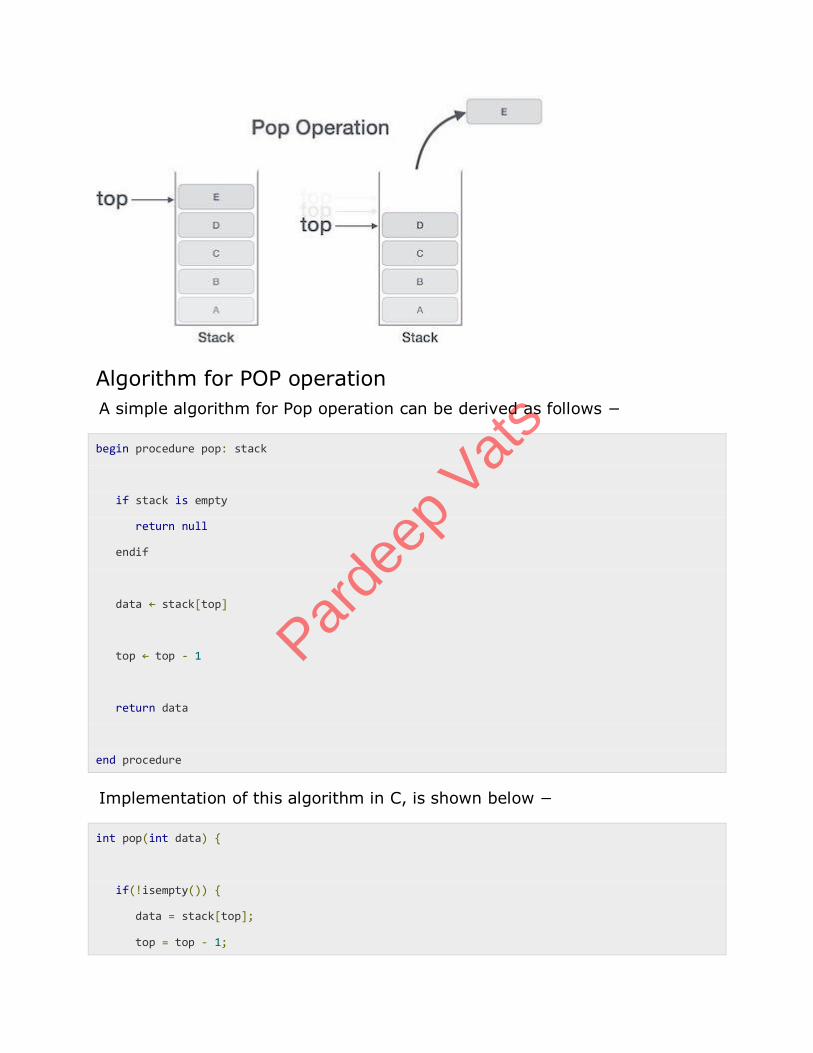
Algorithm for POP operation
A simple algorithm for Pop operation can be derived as follows −
begin procedure pop: stack
if stack is empty
return null
endif
data ← stack[top]
top ← top - 1
return data
end procedure
Implementation of this algorithm in C, is shown below −
int pop(int data) {
if(!isempty()) {
data = stack[top];
top = top - 1;
Parde
ep V
ats
return data;
}
else {
printf("Could not retrieve data, Stack is empty.\n");
}
}
Data Structure - Expression Parsing The way to write arithmetic expression is known as notation. An arithmetic
expression can be written in three different but equivalent notations, i.e.,
without changing the essence or output of expression. These notations are
−
Infix Notation
Prefix (Polish) Notation
Postfix (Reverse-Polish) Notation
These notations are named as how they use operator in expression. We
shall learn the same here in this chapter.
Infix Notation We write expression in infix notation, e.g. a-b+c, where operators are
used in-between operands. It is easy for us humans to read, write and
speak in infix notation but the same does not go well with computing
devices. An algorithm to process infix notation could be difficult and costly
in terms of time and space consumption.
Prefix Notation In this notation, operator is prefixed to operands, i.e. operator is written
ahead of operands. For example +ab. This is equivalent to its infix
notation a+b. Prefix notation is also known as Polish Notation.
Parde
ep V
ats
Postfix Notation This notation style is known as Reversed Polish Notation. In this notation
style, operator is postfixed to the operands i.e., operator is written after
the operands. For example ab+. This is equivalent to its infix notation a+b.
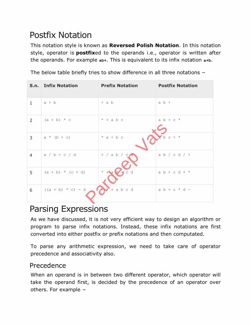
The below table briefly tries to show difference in all three notations −
S.n. Infix Notation Prefix Notation Postfix Notation
1 a + b + a b a b +
2 (a + b) * c * + a b c a b + c *
3 a * (b + c) * a + b c a b c + *
4 a / b + c / d + / a b / c d a b / c d / +
5 (a + b) * (c + d) * + a b + c d a b + c d + *
6 ((a + b) * c) - d - * + a b c d a b + c * d -
Parsing Expressions As we have discussed, it is not very efficient way to design an algorithm or
program to parse infix notations. Instead, these infix notations are first
converted into either postfix or prefix notations and then computated.
To parse any arithmetic expression, we need to take care of operator
precedence and associativity also.
Precedence
When an operand is in between two different operator, which operator will
take the operand first, is decided by the precedence of an operator over
others. For example −
Parde
ep V
ats
As multiplication operation has precedence over addition, b * c will be
evaluated firs. A table of operator precedence is provided later.
Associativity
Associativity describes the rule where operators with same precedence
appear in an expression. For example, in expression a+b−c, both + and −
has same precedence, then which part of expression will be evaluated first,
is determined by associativity of those operators. Here, both + and − are
left associative, so the expression will be evaluated as (a+b)−c.
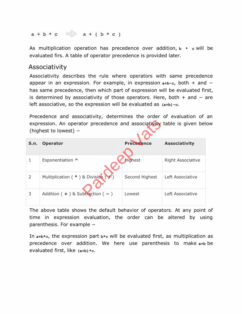
Precedence and associativity, determines the order of evaluation of an
expression. An operator precedence and associativity table is given below
(highest to lowest) −
S.n. Operator Precedence Associativity
1 Esponentiation ^ Highest Right Associative
2 Multiplication ( * ) & Division ( / ) Second Highest Left Associative
3 Addition ( + ) & Subtraction ( − ) Lowest Left Associative
The above table shows the default behavior of operators. At any point of
time in expression evaluation, the order can be altered by using
parenthesis. For example −
In a+b*c, the expression part b*c will be evaluated first, as multiplication as
precedence over addition. We here use parenthesis to make a+b be
evaluated first, like (a+b)*c.
Parde
ep V
ats
Data Structure - Queue Queue is an abstract data structure, somewhat similar to stack. In contrast
to stack, queue is opened at both end. One end is always used to insert
data (enqueue) and the other is used to remove data (dequeue). Queue
follows First-In-First-Out methodology, i.e., the data item stored first will be
accessed first.
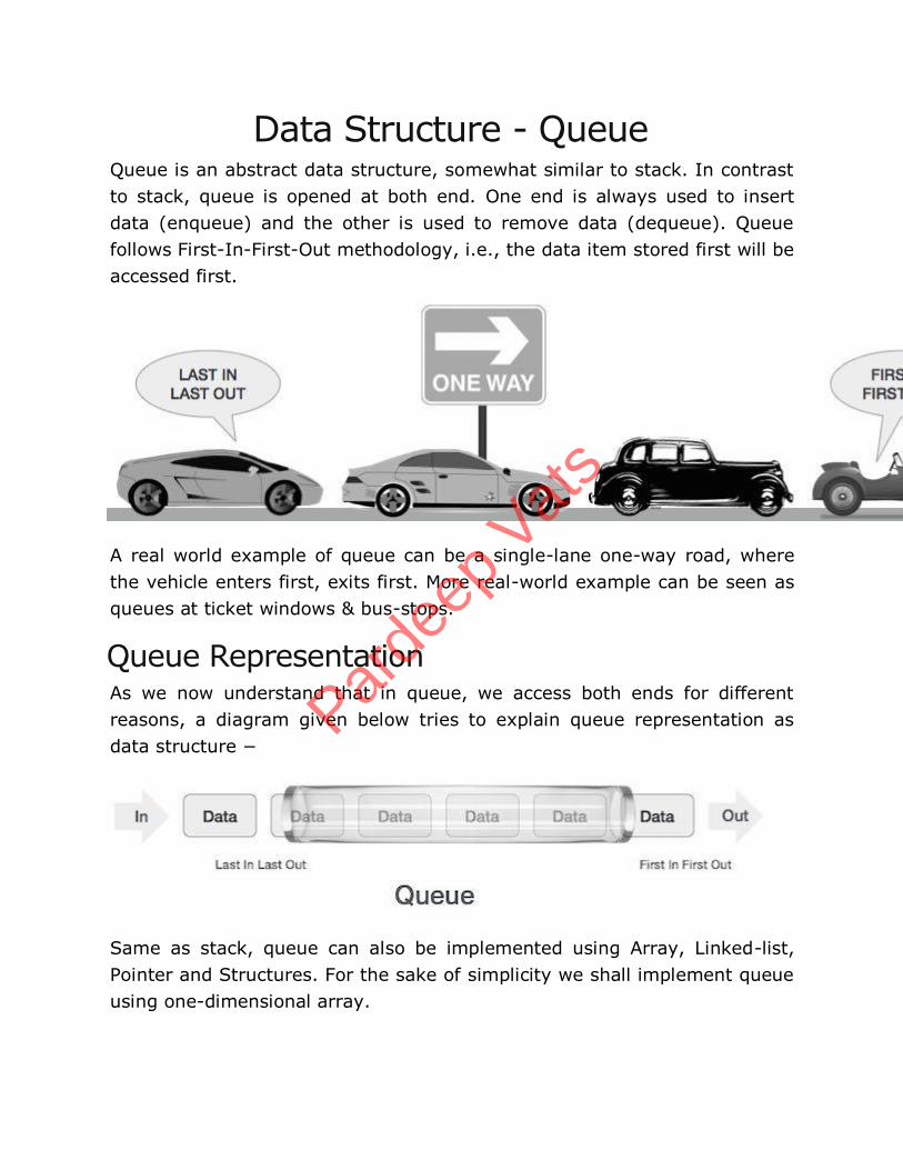
A real world example of queue can be a single-lane one-way road, where
the vehicle enters first, exits first. More real-world example can be seen as
queues at ticket windows & bus-stops.
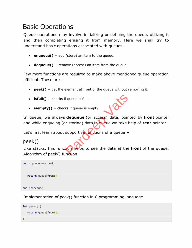
Queue Representation As we now understand that in queue, we access both ends for different
reasons, a diagram given below tries to explain queue representation as
data structure −
Same as stack, queue can also be implemented using Array, Linked-list,
Pointer and Structures. For the sake of simplicity we shall implement queue
using one-dimensional array.
Parde
ep V
ats
Basic Operations Queue operations may involve initializing or defining the queue, utilizing it
and then completing erasing it from memory. Here we shall try to
understand basic operations associated with queues −
enqueue() − add (store) an item to the queue.
dequeue() − remove (access) an item from the queue.
Few more functions are required to make above mentioned queue operation
efficient. These are −
peek() − get the element at front of the queue without removing it.
isfull() − checks if queue is full.
isempty() − checks if queue is empty.
In queue, we always dequeue (or access) data, pointed by front pointer
and while enqueing (or storing) data in queue we take help of rear pointer.
Let's first learn about supportive functions of a queue −
peek()
Like stacks, this function helps to see the data at the front of the queue.
Algorithm of peek() function −
begin procedure peek
return queue[front]
end procedure
Implementation of peek() function in C programming language −
int peek() {
return queue[front];
}
Parde
ep V
ats
isfull()
As we are using single dimension array to implement queue, we just check
for the rear pointer to reach at MAXSIZE to determine that queue is full. In
case we maintain queue in a circular linked-list, the algorithm will differ.
Algorithm of isfull() function −
begin procedure isfull
if rear equals to MAXSIZE
return true
else
return false
endif
end procedure
Implementation of isfull() function in C programming language −
bool isfull() {
if(rear == MAXSIZE - 1)
return true;
else
return false;
}
isempty()
Algorithm of isempty() function −
begin procedure isempty
if front is less than MIN OR front is greater than rear
return true
else
return false
endif
Parde
ep V
ats
end procedure
If value of front is less than MIN or 0, it tells that queue is not yet
initialized, hence empty.
Here's the C programming code −
bool isempty() {
if(front < 0 || front > rear)
return true;
else
return false;
}
Enqueue Operation As queue maintains two data pointers, front and rear, its operations are
comparatively more difficult to implement than stack.
The following steps should be taken to enqueue (insert) data into a queue −
Step 1 − Check if queue is full.
Step 2 − If queue is full, produce overflow error and exit.
Step 3 − If queue is not full, increment rear pointer to point next empty space.
Step 4 − Add data element to the queue location, where rear is pointing.
Step 5 − return success.
Parde
ep V
ats
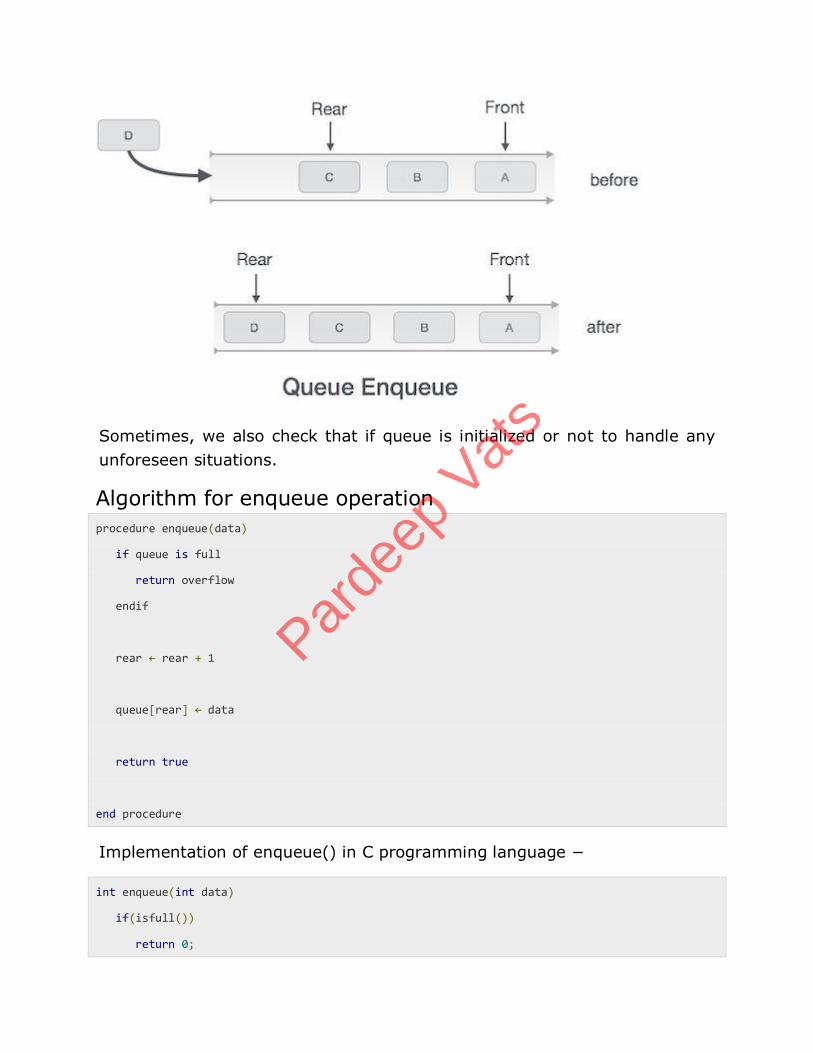
Sometimes, we also check that if queue is initialized or not to handle any
unforeseen situations.
Algorithm for enqueue operation
procedure enqueue(data)
if queue is full
return overflow
endif
rear ← rear + 1
queue[rear] ← data
return true
end procedure
Implementation of enqueue() in C programming language −
int enqueue(int data)
if(isfull())
return 0;
Parde
ep V
ats
rear = rear + 1;
queue[rear] = data;
return 1;
end procedure
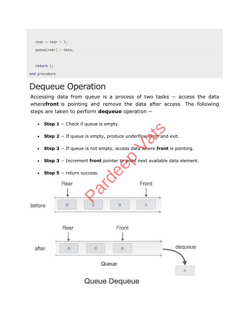
Dequeue Operation Accessing data from queue is a process of two tasks − access the data
wherefront is pointing and remove the data after access. The following
steps are taken to perform dequeue operation −
Step 1 − Check if queue is empty.
Step 2 − If queue is empty, produce underflow error and exit.
Step 3 − If queue is not empty, access data where front is pointing.
Step 3 − Increment front pointer to point next available data element.
Step 5 − return success.
Parde
ep V
ats
Algorithm for dequeue operation −
procedure dequeue
if queue is empty
return underflow
end if
data = queue[front]
front ← front - 1
return true
end procedure
Implementation of dequeue() in C programming language −
int dequeue() {
if(isempty())
return 0;
int data = queue[front];
front = front + 1;
return data;
}
Parde
ep V
ats
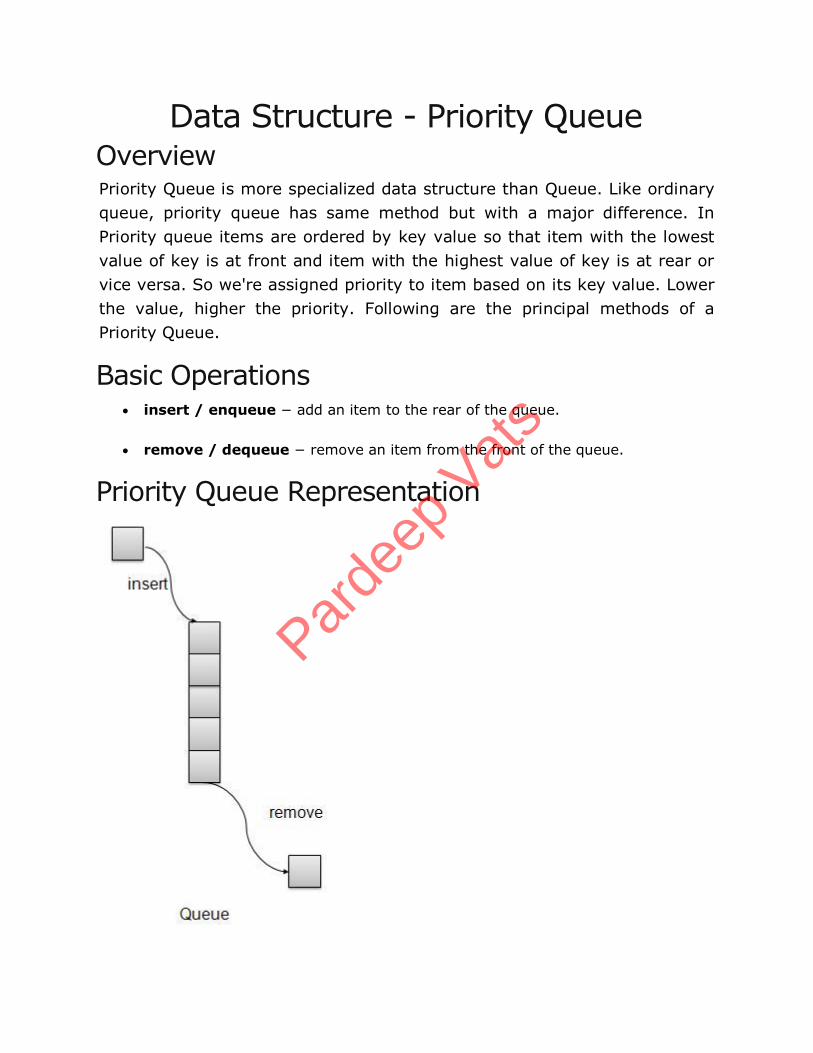
Data Structure - Priority Queue Overview Priority Queue is more specialized data structure than Queue. Like ordinary
queue, priority queue has same method but with a major difference. In
Priority queue items are ordered by key value so that item with the lowest
value of key is at front and item with the highest value of key is at rear or
vice versa. So we're assigned priority to item based on its key value. Lower
the value, higher the priority. Following are the principal methods of a
Priority Queue.
Basic Operations insert / enqueue − add an item to the rear of the queue.
remove / dequeue − remove an item from the front of the queue.
Priority Queue Representation
Parde
ep V
ats
We're going to implement Queue using array in this article. There is few
more operations supported by queue which are following.
Peek − get the element at front of the queue.
isFull − check if queue is full.
isEmpty − check if queue is empty.
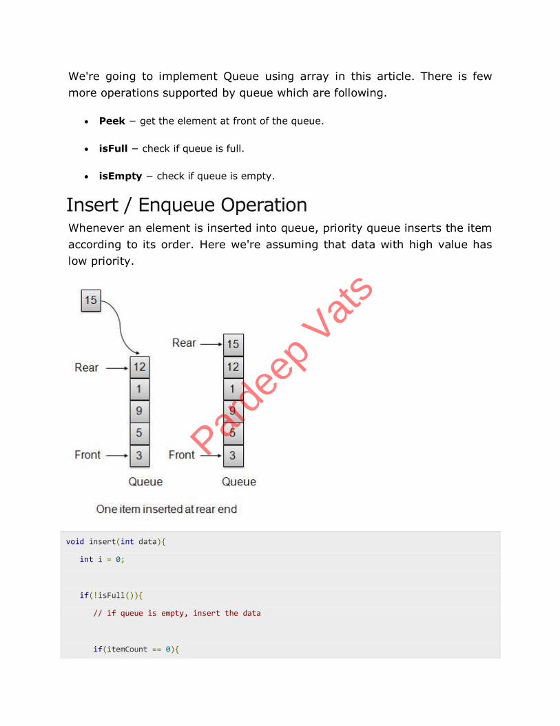
Insert / Enqueue Operation Whenever an element is inserted into queue, priority queue inserts the item
according to its order. Here we're assuming that data with high value has
low priority.
void insert(int data){
int i = 0;
if(!isFull()){
// if queue is empty, insert the data
if(itemCount == 0){
Parde
ep V
ats
intArray[itemCount++] = data;
}else{
// start from the right end of the queue
for(i = itemCount - 1; i >= 0; i-- ){
// if data is larger, shift existing item to right end
if(data > intArray[i]){
intArray[i+1] = intArray[i];
}else{
break;
}
}
// insert the data
intArray[i+1] = data;
itemCount++;
}
}
}
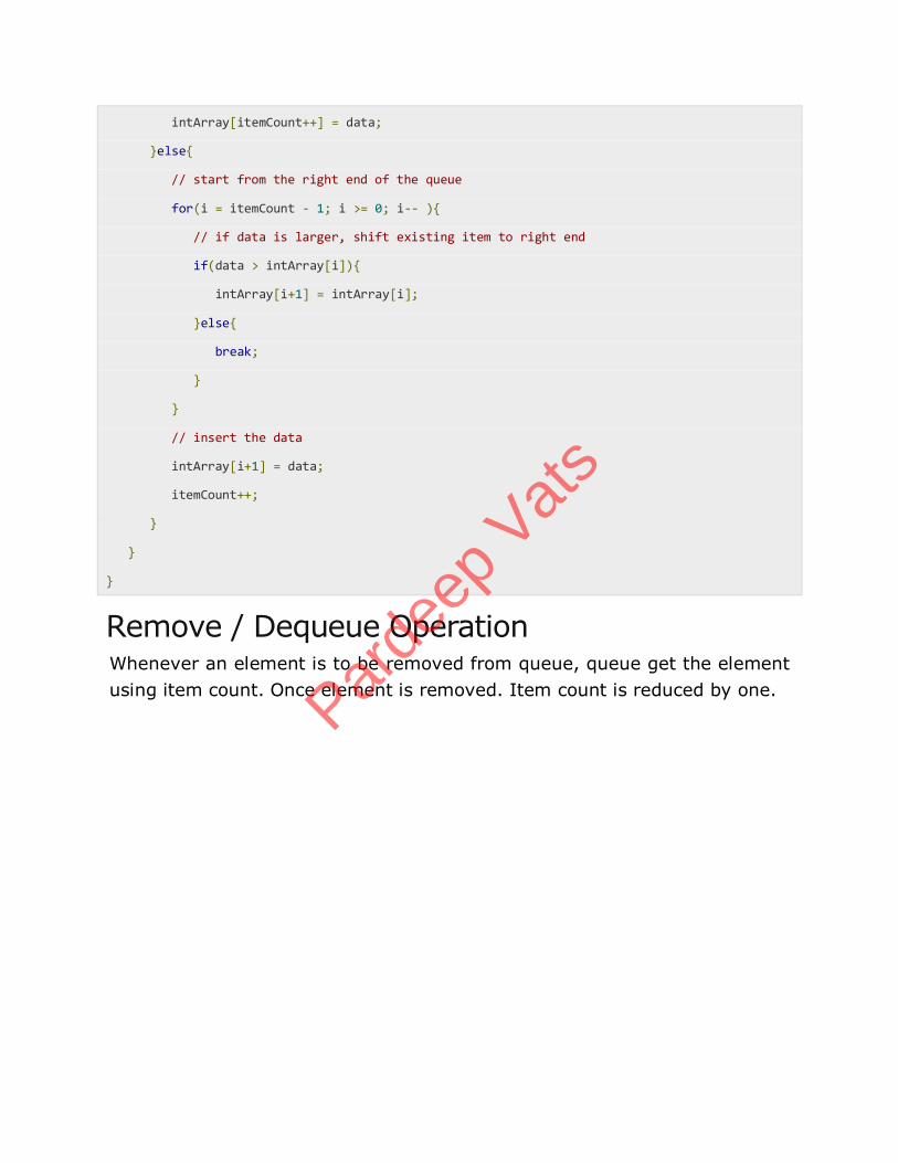
Remove / Dequeue Operation Whenever an element is to be removed from queue, queue get the element
using item count. Once element is removed. Item count is reduced by one.
Parde
ep V
ats
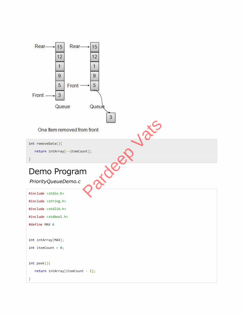
int removeData(){
return intArray[--itemCount];
}
Demo Program PriorityQueueDemo.c
#include <stdio.h>
#include <string.h>
#include <stdlib.h>
#include <stdbool.h>
#define MAX 6
int intArray[MAX];
int itemCount = 0;
int peek(){
return intArray[itemCount - 1];
}
Parde
ep V
ats
bool isEmpty(){
return itemCount == 0;
}
bool isFull(){
return itemCount == MAX;
}
int size(){
return itemCount;
}
void insert(int data){
int i = 0;
if(!isFull()){
// if queue is empty, insert the data
if(itemCount == 0){
intArray[itemCount++] = data;
}else{
// start from the right end of the queue
for(i = itemCount - 1; i >= 0; i-- ){
// if data is larger, shift existing item to right end
if(data > intArray[i]){
intArray[i+1] = intArray[i];
}else{
break;
}
}
// insert the data
Parde
ep V
ats
intArray[i+1] = data;
itemCount++;
}
}
}
int removeData(){
return intArray[--itemCount];
}
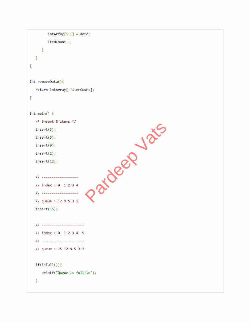
int main() {
/* insert 5 items */
insert(3);
insert(5);
insert(9);
insert(1);
insert(12);
// ------------------
// index : 0 1 2 3 4
// ------------------
// queue : 12 9 5 3 1
insert(15);
// ---------------------
// index : 0 1 2 3 4 5
// ---------------------
// queue : 15 12 9 5 3 1
if(isFull()){
printf("Queue is full!\n");
}
Parde
ep V
ats
// remove one item
int num = removeData();
printf("Element removed: %d\n",num);
// ---------------------
// index : 0 1 2 3 4
// ---------------------
// queue : 15 12 9 5 3
// insert more items
insert(16);
// ----------------------
// index : 0 1 2 3 4 5
// ----------------------
// queue : 16 15 12 9 5 3
// As queue is full, elements will not be inserted.
insert(17);
insert(18);
// ----------------------
// index : 0 1 2 3 4 5
// ----------------------
// queue : 16 15 12 9 5 3
printf("Element at front: %d\n",peek());
printf("----------------------\n");
printf("index : 5 4 3 2 1 0\n");
printf("----------------------\n");
printf("Queue: ");
while(!isEmpty()){
Parde
ep V
ats
int n = removeData();
printf("%d ",n);
}
}
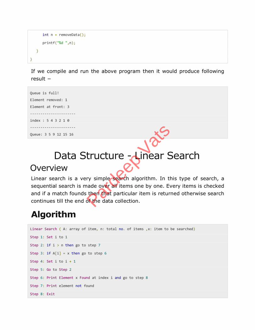
If we compile and run the above program then it would produce following
result −
Queue is full!
Element removed: 1
Element at front: 3
----------------------
index : 5 4 3 2 1 0
----------------------
Queue: 3 5 9 12 15 16
Data Structure - Linear Search Overview Linear search is a very simple search algorithm. In this type of search, a
sequential search is made over all items one by one. Every items is checked
and if a match founds then that particular item is returned otherwise search
continues till the end of the data collection.
Algorithm
Linear Search ( A: array of item, n: total no. of items ,x: item to be searched)
Step 1: Set i to 1
Step 2: if i > n then go to step 7
Step 3: if A[i] = x then go to step 6
Step 4: Set i to i + 1
Step 5: Go to Step 2
Step 6: Print Element x Found at index i and go to step 8
Step 7: Print element not found
Step 8: Exit
Parde
ep V
ats
Data Structure - Binary Search Overview Binary search is a very fast search algorithm. This search algorithm works
on the principle of divide and conquer. For this algorithm to work properly
the data collection should be in sorted form.
Binary search search a particular item by comparing the middle most item
of the collection. If match occurs then index of item is returned. If middle
item is greater than item then item is searched in sub-array to the right of
the middle item other wise item is search in sub-array to the left of the
middle item. This process continues on sub-array as well until the size of
subarray reduces to zero.
Binary search halves the searchable items and thus reduces the count of
comparisons to be made to very less numbers.
Algorithm Binary Search ( A: array of item, n: total no. of items ,x: item to be searched)
Step 1: Set lowerBound = 1
Step 2: Set upperBound = n
Step 3: if upperBound < lowerBound go to step 12
Step 4: set midPoint = ( lowerBound + upperBound ) / 2
Step 5: if A[midPoint] < x
Step 6: set lowerBound = midPoint + 1
Step 7: if A[midPoint] > x
Step 8: set upperBound = midPoint - 1
Step 9 if A[midPoint] = x go to step 11
Step 10: Go to Step 3
Step 11: Print Element x Found at index midPoint and go to step 13
Step 12: Print element not found
Step 13: Exit
Parde
ep V
ats
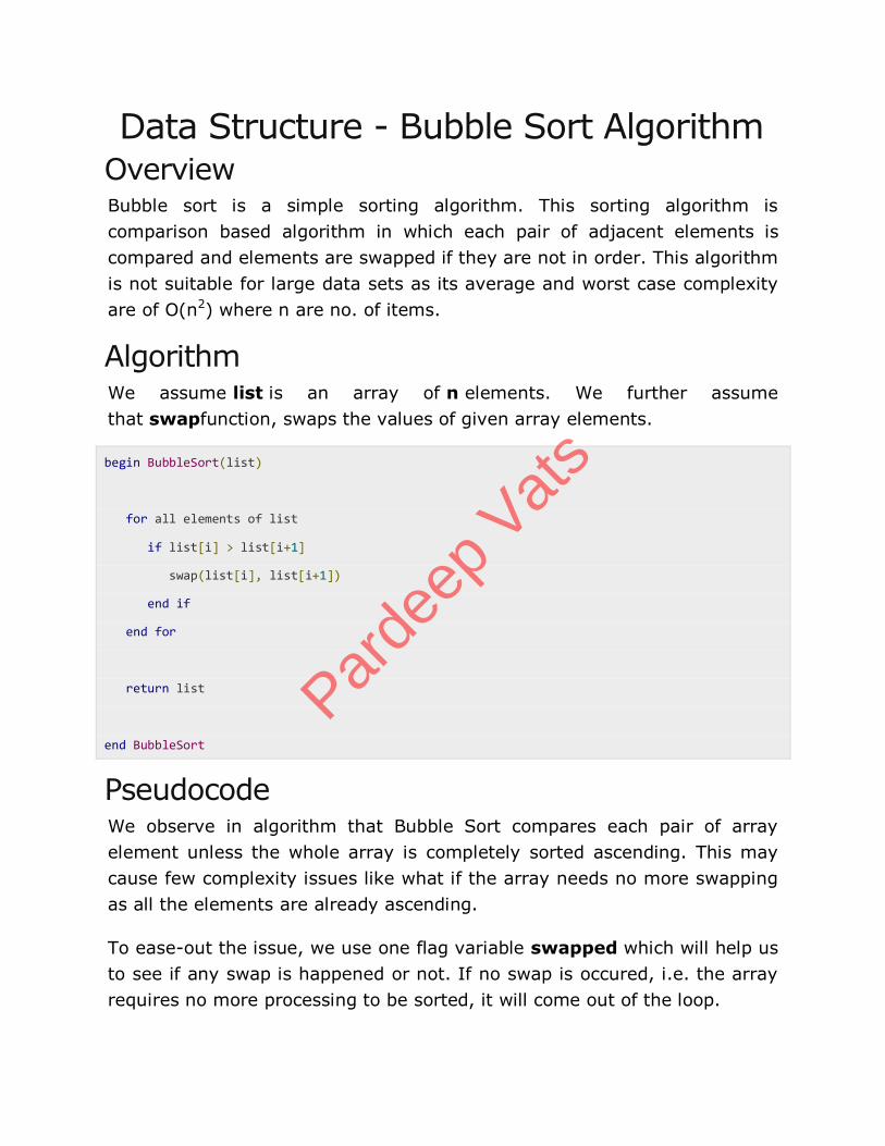
Data Structure - Bubble Sort Algorithm Overview Bubble sort is a simple sorting algorithm. This sorting algorithm is
comparison based algorithm in which each pair of adjacent elements is
compared and elements are swapped if they are not in order. This algorithm
is not suitable for large data sets as its average and worst case complexity
are of O(n2) where n are no. of items.
Algorithm We assume list is an array of n elements. We further assume
that swapfunction, swaps the values of given array elements.
begin BubbleSort(list)
for all elements of list
if list[i] > list[i+1]
swap(list[i], list[i+1])
end if
end for
return list
end BubbleSort
Pseudocode We observe in algorithm that Bubble Sort compares each pair of array
element unless the whole array is completely sorted ascending. This may
cause few complexity issues like what if the array needs no more swapping
as all the elements are already ascending.
To ease-out the issue, we use one flag variable swapped which will help us
to see if any swap is happened or not. If no swap is occured, i.e. the array
requires no more processing to be sorted, it will come out of the loop.
Parde
ep V
ats
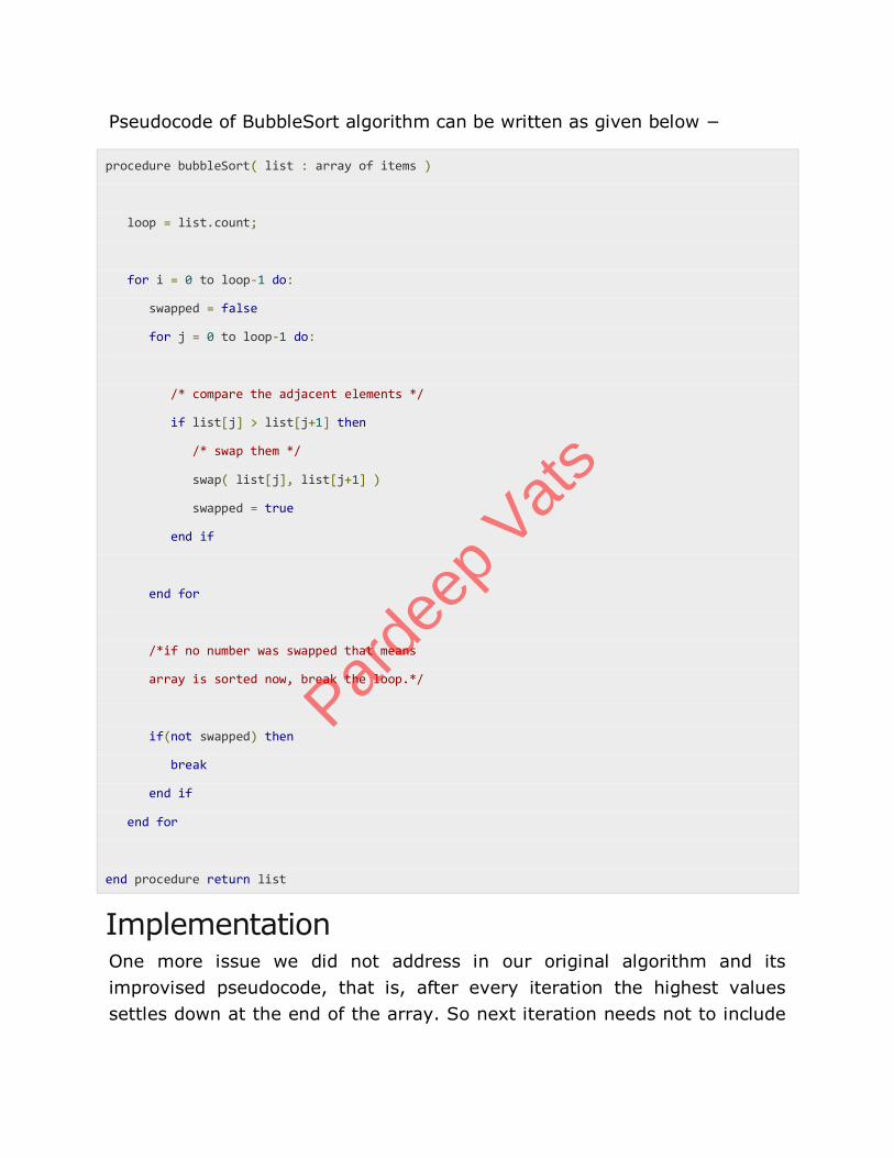
Pseudocode of BubbleSort algorithm can be written as given below −
procedure bubbleSort( list : array of items )
loop = list.count;
for i = 0 to loop-1 do:
swapped = false
for j = 0 to loop-1 do:
/* compare the adjacent elements */
if list[j] > list[j+1] then
/* swap them */
swap( list[j], list[j+1] )
swapped = true
end if
end for
/*if no number was swapped that means
array is sorted now, break the loop.*/
if(not swapped) then
break
end if
end for
end procedure return list
Implementation One more issue we did not address in our original algorithm and its
improvised pseudocode, that is, after every iteration the highest values
settles down at the end of the array. So next iteration needs not to include
Parde
ep V
ats
already sorted elements. For this purpose, in our implementation, we
restrict the inner loop to avoid already sorted values.
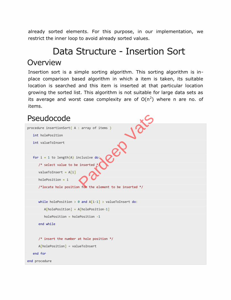
Data Structure - Insertion Sort Overview Insertion sort is a simple sorting algorithm. This sorting algorithm is in-
place comparison based algorithm in which a item is taken, its suitable
location is searched and this item is inserted at that particular location
growing the sorted list. This algorithm is not suitable for large data sets as
its average and worst case complexity are of O(n2) where n are no. of
items.
Pseudocode procedure insertionSort( A : array of items )
int holePosition
int valueToInsert
for i = 1 to length(A) inclusive do:
/* select value to be inserted */
valueToInsert = A[i]
holePosition = i
/*locate hole position for the element to be inserted */
while holePosition > 0 and A[i-1] > valueToInsert do:
A[holePosition] = A[holePosition-1]
holePosition = holePosition -1
end while
/* insert the number at hole position */
A[holePosition] = valueToInsert
end for
end procedure
Parde
ep V
ats
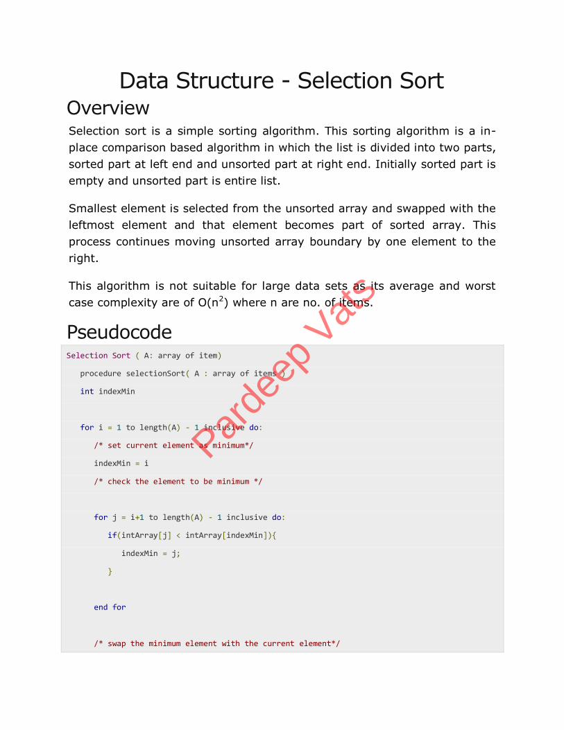
Data Structure - Selection Sort Overview Selection sort is a simple sorting algorithm. This sorting algorithm is a in-
place comparison based algorithm in which the list is divided into two parts,
sorted part at left end and unsorted part at right end. Initially sorted part is
empty and unsorted part is entire list.
Smallest element is selected from the unsorted array and swapped with the
leftmost element and that element becomes part of sorted array. This
process continues moving unsorted array boundary by one element to the
right.
This algorithm is not suitable for large data sets as its average and worst
case complexity are of O(n2) where n are no. of items.
Pseudocode Selection Sort ( A: array of item)
procedure selectionSort( A : array of items )
int indexMin
for i = 1 to length(A) - 1 inclusive do:
/* set current element as minimum*/
indexMin = i
/* check the element to be minimum */
for j = i+1 to length(A) - 1 inclusive do:
if(intArray[j] < intArray[indexMin]){
indexMin = j;
}
end for
/* swap the minimum element with the current element*/
Parde
ep V
ats
if(indexMin != i) then
swap(A[indexMin],A[i])
end if
end for
end procedure
Data Structure - Merge Sort Algorithm Sorting refers to arranging data in a particular format. Sorting
algorithm specifies the way to arrange data in a particular order. Most
common orders are numerical or lexicographical order.
Importance of sorting lies in the fact that data searching can be optimized
to a very high level if data is stored in a sorted manner. Sorting is also used
to represent data in more readable formats. Some of the examples of
sorting in real life scenarios are following.
#include <stdio.h>
int a[20], b[20], n;
void merging(int low, int mid, int high) {
int l1,l2,i;
for(l1 = low, l2 = mid + 1, i = low; l1 <= mid && l2 <= high; i++){
if(a[l1] <= a[l2])
b[i] = a[l1++];
else
b[i] = a[l2++];
}
while(l1 <= mid)
b[i++] = a[l1++];
Parde
ep V
ats
while(l2 <= high)
b[i++] = a[l2++];
for(i = low; i <= high; i++)
a[i] = b[i];
}
void sort(int low,int high) {
int mid;
if(low < high) {
mid = (low+high) / 2;
sort(low, mid);
sort(mid+1, high);
merging(low, mid, high);
}
else {
return;
}
}
int main() {
int i;
printf("Enter N ");
scanf("%d",&n);
printf("Enter elements\n");
for(i = 1; i <= n; i++)
scanf("%d",& a[i]);
Parde
ep V
ats
sort(1,n);
printf("After sorting\n");
for(i = 1; i <= n; i++)
printf("%d\n", a[i]);
}
Data Structure - Shell Sort Overview Shell sort is a highly efficient sorting algorithm and is based on insertion
sort algorithm. This algorithm avoids large shifts as in case of insertion sort
if smaller value is very far right and have to move to far left. This algorithm
uses insertion sort on widely spread elements first to sort them and then
sorts the less widely spaced elements. This spacing is termed as interval.
This interval is calculated based on Knuth's formula as (h=h*3 +1) where h
is interval and initial value is 1. This algorithm is quite efficient for medium
sized data sets as its average and worst case complexity are of O(n) where
n are no. of items.
Pseudocode procedure shellSort( A : array of items )
int innerPosition, outerPosition
int valueToInsert, interval = 1
/* calculate interval*/
while interval < A.length /3 do:
interval = interval * 3 +1
while interval > 0 do:
for outer = interval; outer < A.length; outer ++ do:
/* select value to be inserted */
Parde
ep V
ats
valueToInsert = A[outer]
inner = outer;
/*shift element towards right*/
while inner > interval -1 && A[inner - interval] >= valueToInsert do:
A[inner] = A[inner-1]
inner = inner - interval
end while
/* insert the number at hole position */
A[inner] = valueToInsert
end for
/* calculate interval*/
interval = (interval -1) /3;
end while
end procedure
#include <stdio.h>
#include <stdbool.h>
#define MAX 7
int intArray[MAX] = {4,6,3,2,1,9,7};
void printline(int count){
int i;
for(i = 0;i <count-1;i++){
printf("=");
}
printf("=\n");
}
Parde
ep V
ats
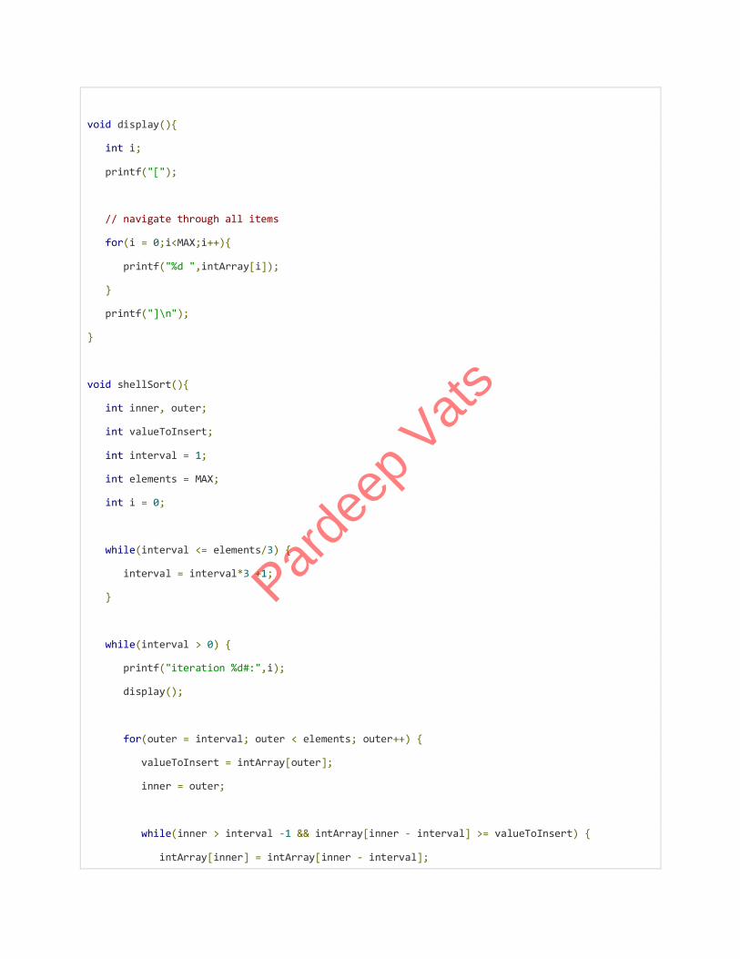
void display(){
int i;
printf("[");
// navigate through all items
for(i = 0;i<MAX;i++){
printf("%d ",intArray[i]);
}
printf("]\n");
}
void shellSort(){
int inner, outer;
int valueToInsert;
int interval = 1;
int elements = MAX;
int i = 0;
while(interval <= elements/3) {
interval = interval*3 +1;
}
while(interval > 0) {
printf("iteration %d#:",i);
display();
for(outer = interval; outer < elements; outer++) {
valueToInsert = intArray[outer];
inner = outer;
while(inner > interval -1 && intArray[inner - interval] >= valueToInsert) {
intArray[inner] = intArray[inner - interval];
Parde
ep V
ats
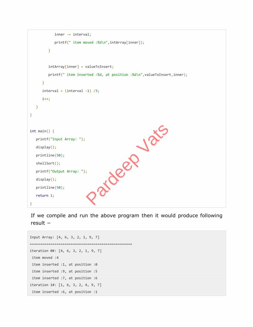
inner -= interval;
printf(" item moved :%d\n",intArray[inner]);
}
intArray[inner] = valueToInsert;
printf(" item inserted :%d, at position :%d\n",valueToInsert,inner);
}
interval = (interval -1) /3;
i++;
}
}
int main() {
printf("Input Array: ");
display();
printline(50);
shellSort();
printf("Output Array: ");
display();
printline(50);
return 1;
}
If we compile and run the above program then it would produce following
result −
Input Array: [4, 6, 3, 2, 1, 9, 7]
==================================================
iteration 0#: [4, 6, 3, 2, 1, 9, 7]
item moved :4
item inserted :1, at position :0
item inserted :9, at position :5
item inserted :7, at position :6
iteration 1#: [1, 6, 3, 2, 4, 9, 7]
item inserted :6, at position :1
Parde
ep V
ats
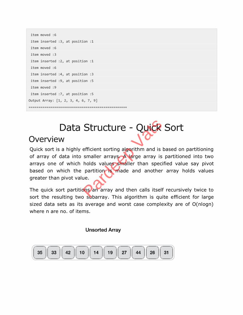
item moved :6
item inserted :3, at position :1
item moved :6
item moved :3
item inserted :2, at position :1
item moved :6
item inserted :4, at position :3
item inserted :9, at position :5
item moved :9
item inserted :7, at position :5
Output Array: [1, 2, 3, 4, 6, 7, 9]
==================================================
Data Structure - Quick Sort Overview Quick sort is a highly efficient sorting algorithm and is based on partitioning
of array of data into smaller arrays. A large array is partitioned into two
arrays one of which holds values smaller than specified value say pivot
based on which the partition is made and another array holds values
greater than pivot value.
The quick sort partitions an array and then calls itself recursively twice to
sort the resulting two subarray. This algorithm is quite efficient for large
sized data sets as its average and worst case complexity are of O(nlogn)
where n are no. of items.
Parde
ep V
ats
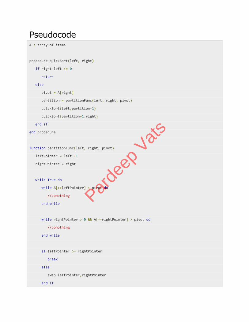
Pseudocode A : array of items
procedure quickSort(left, right)
if right-left <= 0
return
else
pivot = A[right]
partition = partitionFunc(left, right, pivot)
quickSort(left,partition-1)
quickSort(partition+1,right)
end if
end procedure
function partitionFunc(left, right, pivot)
leftPointer = left -1
rightPointer = right
while True do
while A[++leftPointer] < pivot do
//donothing
end while
while rightPointer > 0 && A[--rightPointer] > pivot do
//donothing
end while
if leftPointer >= rightPointer
break
else
swap leftPointer,rightPointer
end if
Parde
ep V
ats
end while
swap leftPointer,right
return leftPointer
end function
procedure swap (num1, num2)
temp = A[num1]
A[num1] = A[num2]
A[num2] = temp;
end procedure
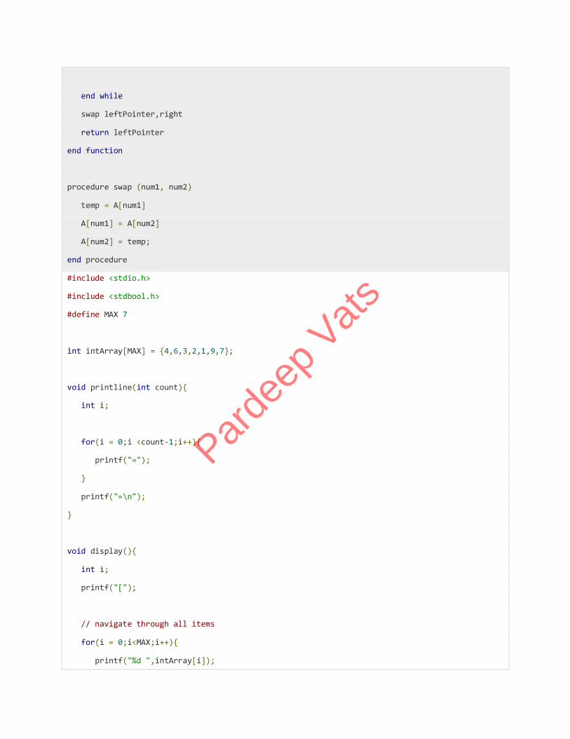
#include <stdio.h>
#include <stdbool.h>
#define MAX 7
int intArray[MAX] = {4,6,3,2,1,9,7};
void printline(int count){
int i;
for(i = 0;i <count-1;i++){
printf("=");
}
printf("=\n");
}
void display(){
int i;
printf("[");
// navigate through all items
for(i = 0;i<MAX;i++){
printf("%d ",intArray[i]);
Parde
ep V
ats
}
printf("]\n");
}
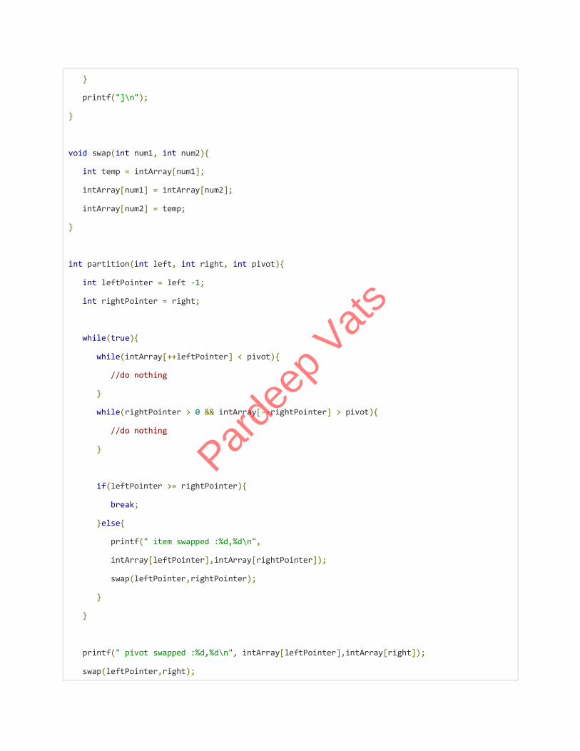
void swap(int num1, int num2){
int temp = intArray[num1];
intArray[num1] = intArray[num2];
intArray[num2] = temp;
}
int partition(int left, int right, int pivot){
int leftPointer = left -1;
int rightPointer = right;
while(true){
while(intArray[++leftPointer] < pivot){
//do nothing
}
while(rightPointer > 0 && intArray[--rightPointer] > pivot){
//do nothing
}
if(leftPointer >= rightPointer){
break;
}else{
printf(" item swapped :%d,%d\n",
intArray[leftPointer],intArray[rightPointer]);
swap(leftPointer,rightPointer);
}
}
printf(" pivot swapped :%d,%d\n", intArray[leftPointer],intArray[right]);
swap(leftPointer,right);
Parde
ep V
ats
printf("Updated Array: ");
display();
return leftPointer;
}
void quickSort(int left, int right){
if(right-left <= 0){
return;
}else{
int pivot = intArray[right];
int partitionPoint = partition(left, right, pivot);
quickSort(left,partitionPoint-1);
quickSort(partitionPoint+1,right);
}
}
main(){
printf("Input Array: ");
display();
printline(50);
quickSort(0,MAX-1);
printf("Output Array: ");
display();
printline(50);
}
If we compile and run the above program then it would produce following
result −
Input Array: [4 6 3 2 1 9 7 ]
==================================================
pivot swapped :9,7
Updated Array: [4 6 3 2 1 7 9 ]
pivot swapped :4,1
Parde
ep V
ats
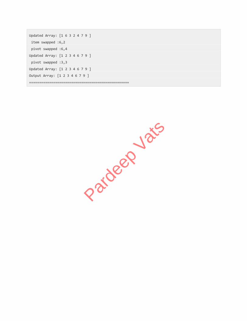
Updated Array: [1 6 3 2 4 7 9 ]
item swapped :6,2
pivot swapped :6,4
Updated Array: [1 2 3 4 6 7 9 ]
pivot swapped :3,3
Updated Array: [1 2 3 4 6 7 9 ]
Output Array: [1 2 3 4 6 7 9 ]
==================================================
Parde
ep V
ats
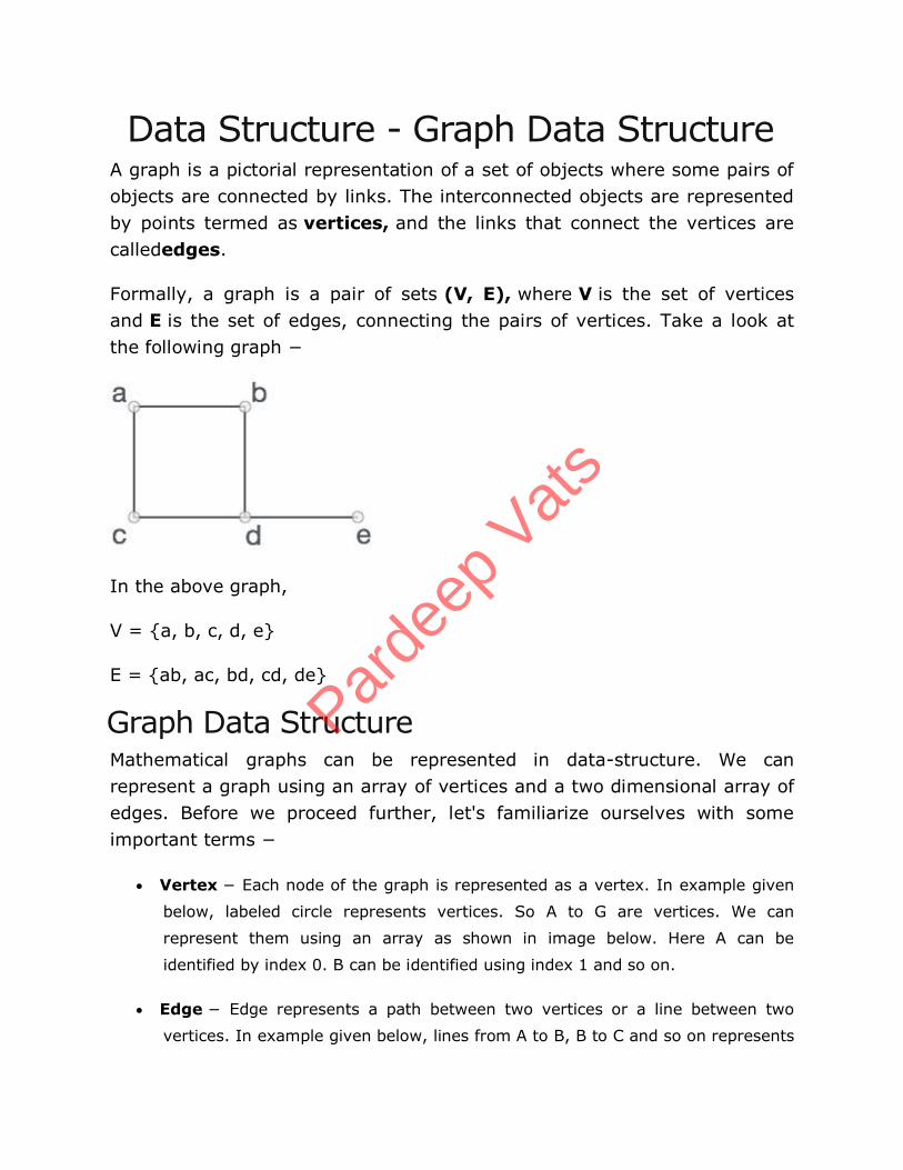
Data Structure - Graph Data Structure A graph is a pictorial representation of a set of objects where some pairs of
objects are connected by links. The interconnected objects are represented
by points termed as vertices, and the links that connect the vertices are
callededges.
Formally, a graph is a pair of sets (V, E), where V is the set of vertices
and E is the set of edges, connecting the pairs of vertices. Take a look at
the following graph −
In the above graph,
V = {a, b, c, d, e}
E = {ab, ac, bd, cd, de}
Graph Data Structure Mathematical graphs can be represented in data-structure. We can
represent a graph using an array of vertices and a two dimensional array of
edges. Before we proceed further, let's familiarize ourselves with some
important terms −
Vertex − Each node of the graph is represented as a vertex. In example given
below, labeled circle represents vertices. So A to G are vertices. We can
represent them using an array as shown in image below. Here A can be
identified by index 0. B can be identified using index 1 and so on.
Edge − Edge represents a path between two vertices or a line between two
vertices. In example given below, lines from A to B, B to C and so on represents
Parde
ep V
ats
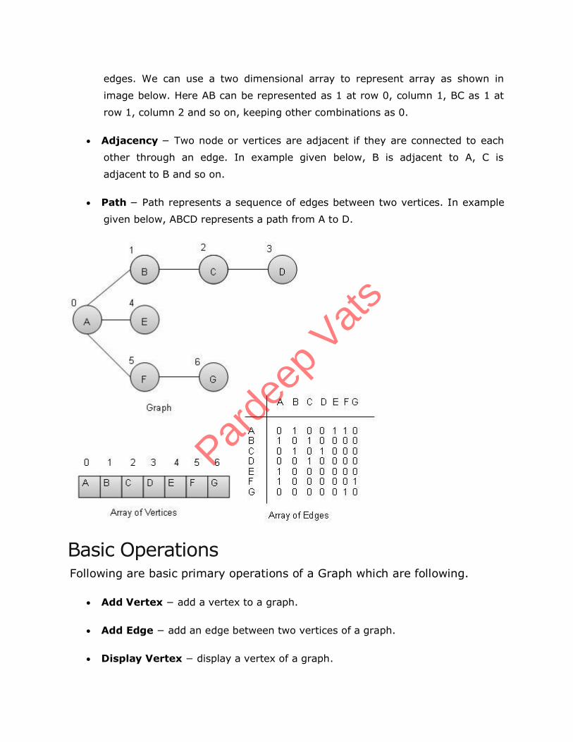
edges. We can use a two dimensional array to represent array as shown in
image below. Here AB can be represented as 1 at row 0, column 1, BC as 1 at
row 1, column 2 and so on, keeping other combinations as 0.
Adjacency − Two node or vertices are adjacent if they are connected to each
other through an edge. In example given below, B is adjacent to A, C is
adjacent to B and so on.
Path − Path represents a sequence of edges between two vertices. In example
given below, ABCD represents a path from A to D.
Basic Operations Following are basic primary operations of a Graph which are following.
Add Vertex − add a vertex to a graph.
Add Edge − add an edge between two vertices of a graph.
Display Vertex − display a vertex of a graph.
Parde
ep V
ats
Add Vertex Operation //add vertex to the vertex list
void addVertex(char label){
struct vertex* vertex = (struct vertex*) malloc(sizeof(struct vertex));
vertex->label = label;
vertex->visited = false;
lstVertices[vertexCount++] = vertex;
}
Add Edge Operation //add edge to edge array
void addEdge(int start,int end){
adjMatrix[start][end] = 1;
adjMatrix[end][start] = 1;
}
Display Edge Operation //display the vertex
void displayVertex(int vertexIndex){
printf("%c ",lstVertices[vertexIndex]->label);
}
Data Structure - Depth First Traversal Depth First Search Algorithm Depth First Search algorithm(DFS) traverses a graph in a depthward motion
and uses a stack to remember to get the next vertex to start a search when
a dead end occurs in any iteration.
Parde
ep V
ats
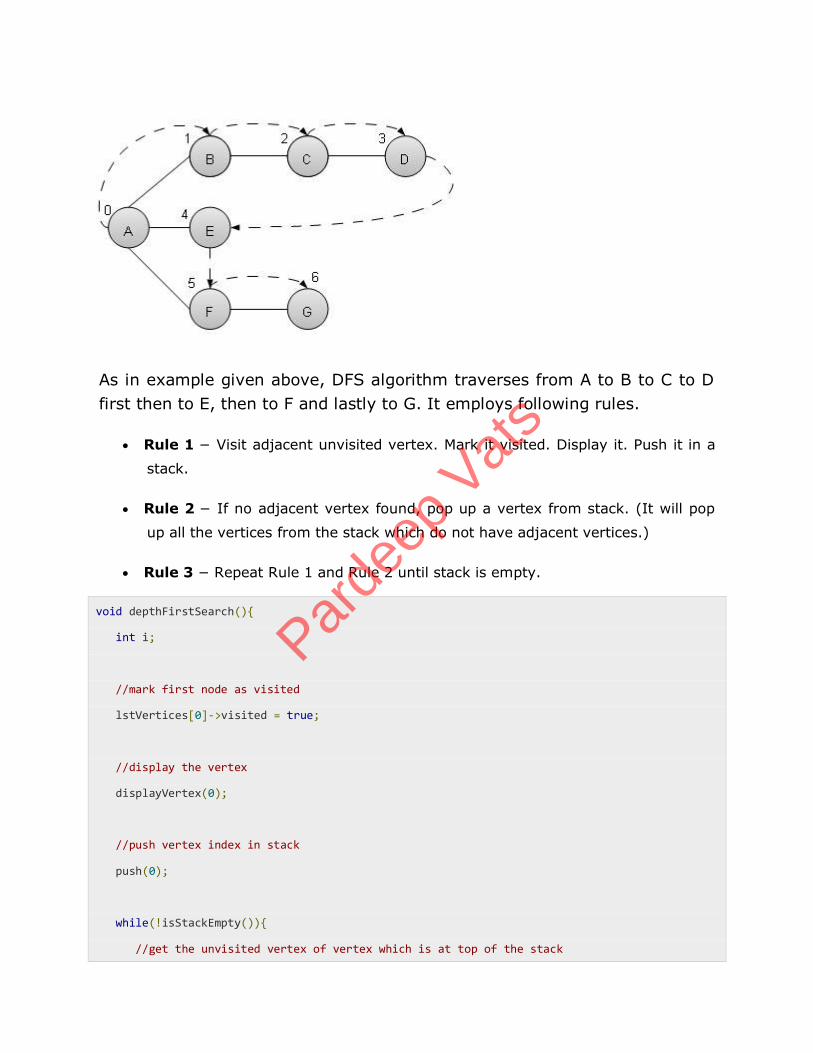
As in example given above, DFS algorithm traverses from A to B to C to D
first then to E, then to F and lastly to G. It employs following rules.
Rule 1 − Visit adjacent unvisited vertex. Mark it visited. Display it. Push it in a
stack.
Rule 2 − If no adjacent vertex found, pop up a vertex from stack. (It will pop
up all the vertices from the stack which do not have adjacent vertices.)
Rule 3 − Repeat Rule 1 and Rule 2 until stack is empty.
void depthFirstSearch(){
int i;
//mark first node as visited
lstVertices[0]->visited = true;
//display the vertex
displayVertex(0);
//push vertex index in stack
push(0);
while(!isStackEmpty()){
//get the unvisited vertex of vertex which is at top of the stack
Parde
ep V
ats
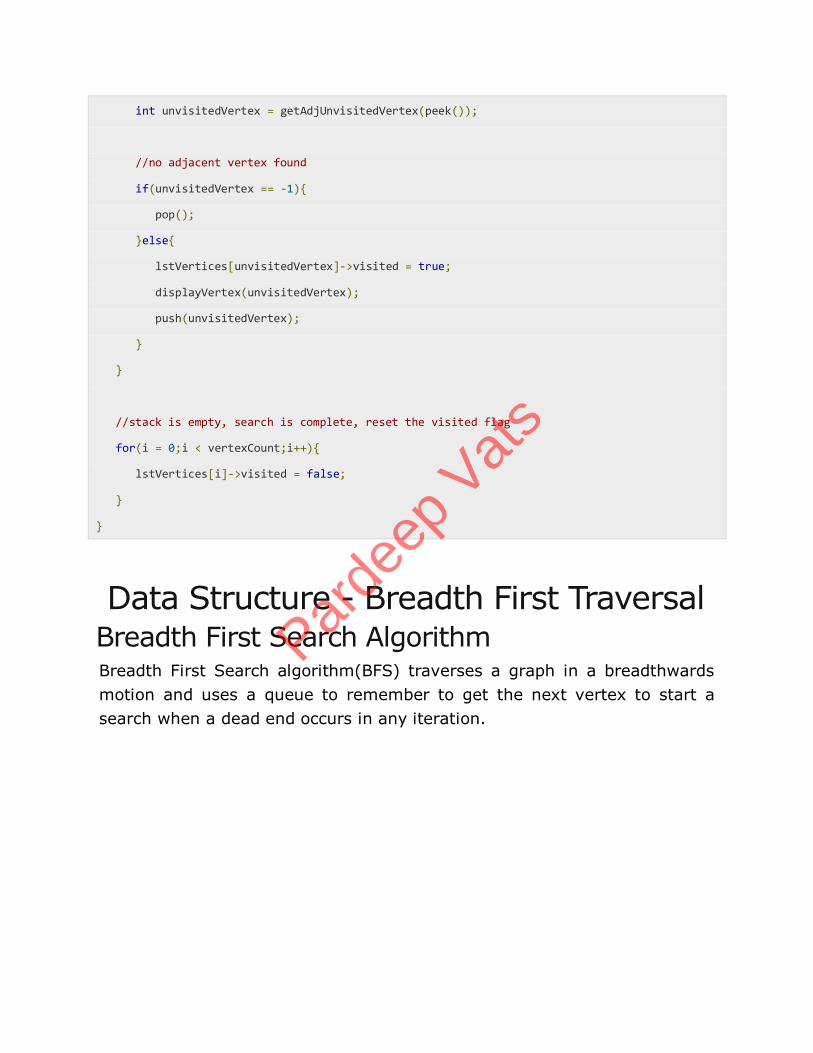
int unvisitedVertex = getAdjUnvisitedVertex(peek());
//no adjacent vertex found
if(unvisitedVertex == -1){
pop();
}else{
lstVertices[unvisitedVertex]->visited = true;
displayVertex(unvisitedVertex);
push(unvisitedVertex);
}
}
//stack is empty, search is complete, reset the visited flag
for(i = 0;i < vertexCount;i++){
lstVertices[i]->visited = false;
}
}
Data Structure - Breadth First Traversal Breadth First Search Algorithm Breadth First Search algorithm(BFS) traverses a graph in a breadthwards
motion and uses a queue to remember to get the next vertex to start a
search when a dead end occurs in any iteration.
Parde
ep V
ats
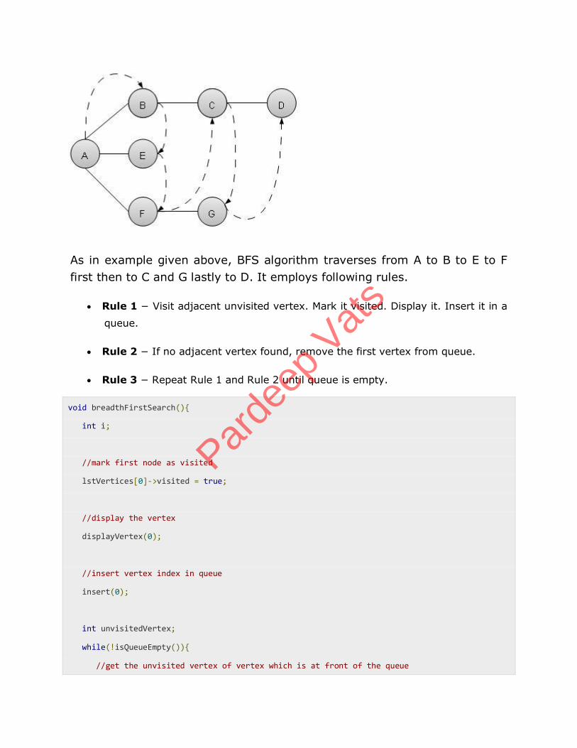
As in example given above, BFS algorithm traverses from A to B to E to F
first then to C and G lastly to D. It employs following rules.
Rule 1 − Visit adjacent unvisited vertex. Mark it visited. Display it. Insert it in a
queue.
Rule 2 − If no adjacent vertex found, remove the first vertex from queue.
Rule 3 − Repeat Rule 1 and Rule 2 until queue is empty.
void breadthFirstSearch(){
int i;
//mark first node as visited
lstVertices[0]->visited = true;
//display the vertex
displayVertex(0);
//insert vertex index in queue
insert(0);
int unvisitedVertex;
while(!isQueueEmpty()){
//get the unvisited vertex of vertex which is at front of the queue
Parde
ep V
ats
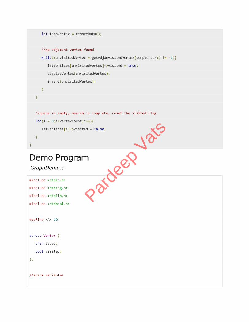
int tempVertex = removeData();
//no adjacent vertex found
while((unvisitedVertex = getAdjUnvisitedVertex(tempVertex)) != -1){
lstVertices[unvisitedVertex]->visited = true;
displayVertex(unvisitedVertex);
insert(unvisitedVertex);
}
}
//queue is empty, search is complete, reset the visited flag
for(i = 0;i<vertexCount;i++){
lstVertices[i]->visited = false;
}
}
Demo Program GraphDemo.c
#include <stdio.h>
#include <string.h>
#include <stdlib.h>
#include <stdbool.h>
#define MAX 10
struct Vertex {
char label;
bool visited;
};
//stack variables
Parde
ep V
ats
int stack[MAX];
int top = -1;
//queue variables
int queue[MAX];
int rear = -1;
int front = 0;
int queueItemCount = 0;
//graph variables
//array of vertices
struct Vertex* lstVertices[MAX];
//adjacency matrix
int adjMatrix[MAX][MAX];
//vertex count
int vertexCount = 0;
//stack functions
void push(int item) {
stack[++top] = item;
}
int pop() {
return stack[top--];
}
int peek() {
return stack[top];
Parde
ep V
ats
}
bool isStackEmpty(){
return top == -1;
}
//queue functions
void insert(int data){
queue[++rear] = data;
queueItemCount++;
}
int removeData(){
queueItemCount--;
return queue[front++];
}
bool isQueueEmpty(){
return queueItemCount == 0;
}
//graph functions
//add vertex to the vertex list
void addVertex(char label){
struct Vertex* vertex = (struct Vertex*) malloc(sizeof(struct Vertex));
vertex->label = label;
vertex->visited = false;
lstVertices[vertexCount++] = vertex;
}
//add edge to edge array
Parde
ep V
ats
void addEdge(int start,int end){
adjMatrix[start][end] = 1;
adjMatrix[end][start] = 1;
}
//display the vertex
void displayVertex(int vertexIndex){
printf("%c ",lstVertices[vertexIndex]->label);
}
//get the adjacent unvisited vertex
int getAdjUnvisitedVertex(int vertexIndex){
int i;
for(i = 0; i<vertexCount; i++)
if(adjMatrix[vertexIndex][i] == 1 && lstVertices[i]->visited == false)
return i;
return -1;
}
void depthFirstSearch(){
int i;
//mark first node as visited
lstVertices[0]->visited = true;
//display the vertex
displayVertex(0);
//push vertex index in stack
push(0);
while(!isStackEmpty()){
Parde
ep V
ats
//get the unvisited vertex of vertex which is at top of the stack
int unvisitedVertex = getAdjUnvisitedVertex(peek());
//no adjacent vertex found
if(unvisitedVertex == -1){
pop();
}else{
lstVertices[unvisitedVertex]->visited = true;
displayVertex(unvisitedVertex);
push(unvisitedVertex);
}
}
//stack is empty, search is complete, reset the visited flag
for(i = 0;i < vertexCount;i++){
lstVertices[i]->visited = false;
}
}
void breadthFirstSearch(){
int i;
//mark first node as visited
lstVertices[0]->visited = true;
//display the vertex
displayVertex(0);
//insert vertex index in queue
insert(0);
int unvisitedVertex;
while(!isQueueEmpty()){
Parde
ep V
ats
//get the unvisited vertex of vertex which is at front of the queue
int tempVertex = removeData();
//no adjacent vertex found
while((unvisitedVertex = getAdjUnvisitedVertex(tempVertex)) != -1){
lstVertices[unvisitedVertex]->visited = true;
displayVertex(unvisitedVertex);
insert(unvisitedVertex);
}
}
//queue is empty, search is complete, reset the visited flag
for(i = 0;i<vertexCount;i++){
lstVertices[i]->visited = false;
}
}
main() {
int i, j;
for(i = 0; i<MAX; i++) // set adjacency
for(j = 0; j<MAX; j++) // matrix to 0
adjMatrix[i][j] = 0;
addVertex('A'); //0
addVertex('B'); //1
addVertex('C'); //2
addVertex('D'); //3
addVertex('E'); //4
addVertex('F'); //5
addVertex('G'); //6
/* 1 2 3
Parde
ep V
ats
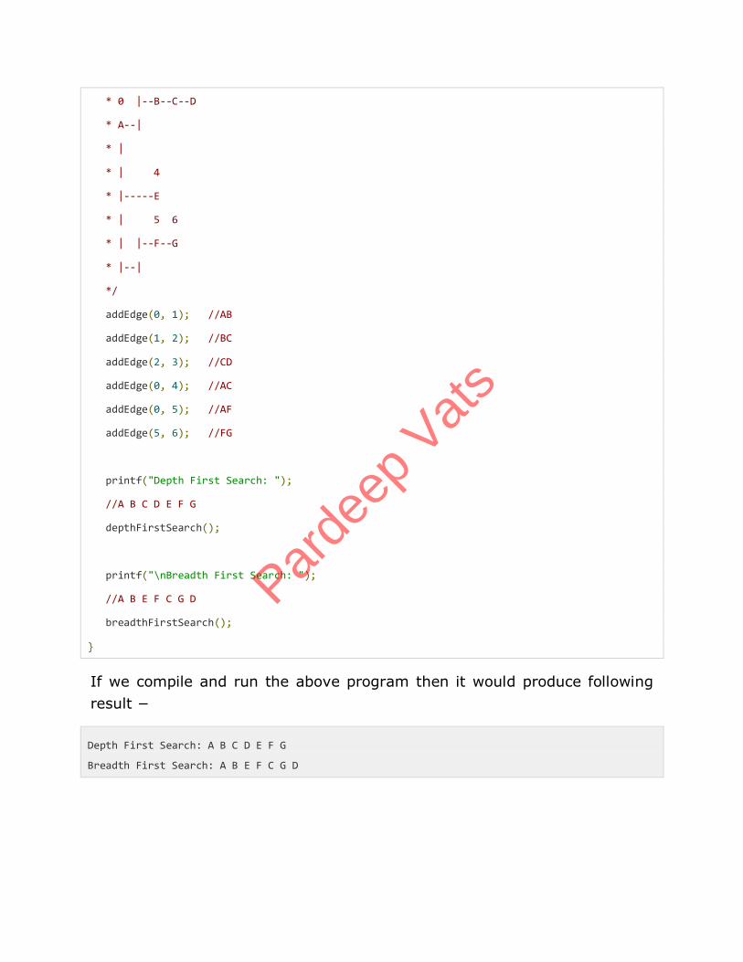
* 0 |--B--C--D
* A--|
* |
* | 4
* |-----E
* | 5 6
* | |--F--G
* |--|
*/
addEdge(0, 1); //AB
addEdge(1, 2); //BC
addEdge(2, 3); //CD
addEdge(0, 4); //AC
addEdge(0, 5); //AF
addEdge(5, 6); //FG
printf("Depth First Search: ");
//A B C D E F G
depthFirstSearch();
printf("\nBreadth First Search: ");
//A B E F C G D
breadthFirstSearch();
}
If we compile and run the above program then it would produce following
result −
Depth First Search: A B C D E F G
Breadth First Search: A B E F C G D
Parde
ep V
ats
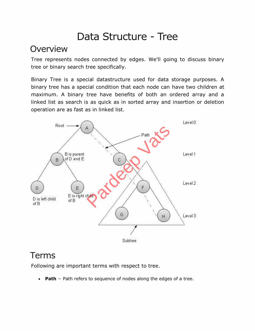
Data Structure - Tree Overview Tree represents nodes connected by edges. We'll going to discuss binary
tree or binary search tree specifically.
Binary Tree is a special datastructure used for data storage purposes. A
binary tree has a special condition that each node can have two children at
maximum. A binary tree have benefits of both an ordered array and a
linked list as search is as quick as in sorted array and insertion or deletion
operation are as fast as in linked list.
Terms Following are important terms with respect to tree.
Path − Path refers to sequence of nodes along the edges of a tree.
Parde
ep V
ats
Root − Node at the top of the tree is called root. There is only one root per tree
and one path from root node to any node.
Parent − Any node except root node has one edge upward to a node called
parent.
Child − Node below a given node connected by its edge downward is called its
child node.
Leaf − Node which does not have any child node is called leaf node.
Subtree − Subtree represents descendents of a node.
Visiting − Visiting refers to checking value of a node when control is on the
node.
Traversing − Traversing means passing through nodes in a specific order.
Levels − Level of a node represents the generation of a node. If root node is at
level 0, then its next child node is at level 1, its grandchild is at level 2 and so
on.
keys − Key represents a value of a node based on which a search operation is
to be carried out for a node.
Binary Search tree exhibits a special behaviour. A node's left child must
have value less than its parent's value and node's right child must have
value greater than it's parent value.
Parde
ep V
ats
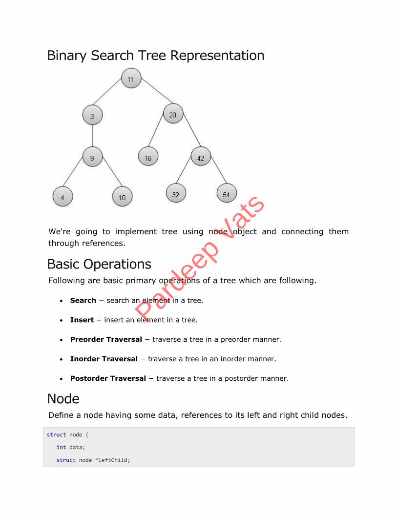
Binary Search Tree Representation
We're going to implement tree using node object and connecting them
through references.
Basic Operations Following are basic primary operations of a tree which are following.
Search − search an element in a tree.
Insert − insert an element in a tree.
Preorder Traversal − traverse a tree in a preorder manner.
Inorder Traversal − traverse a tree in an inorder manner.
Postorder Traversal − traverse a tree in a postorder manner.
Node Define a node having some data, references to its left and right child nodes.
struct node {
int data;
struct node *leftChild;
Parde
ep V
ats
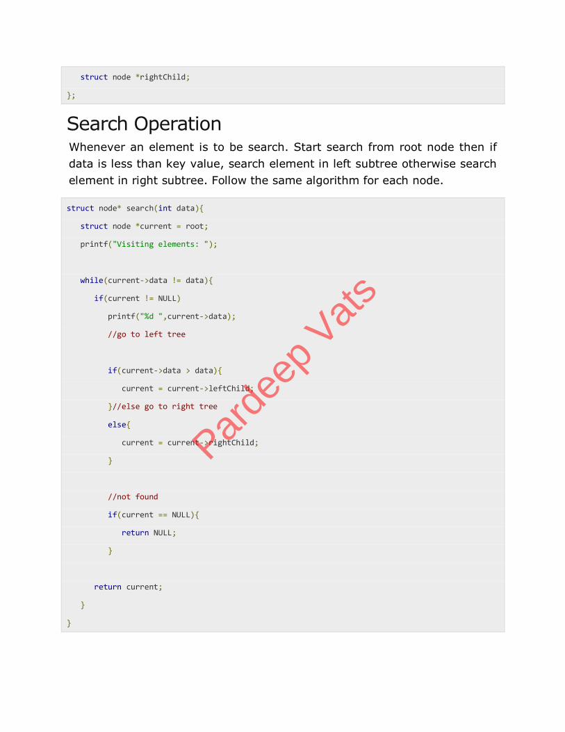
struct node *rightChild;
};
Search Operation Whenever an element is to be search. Start search from root node then if
data is less than key value, search element in left subtree otherwise search
element in right subtree. Follow the same algorithm for each node.
struct node* search(int data){
struct node *current = root;
printf("Visiting elements: ");
while(current->data != data){
if(current != NULL)
printf("%d ",current->data);
//go to left tree
if(current->data > data){
current = current->leftChild;
}//else go to right tree
else{
current = current->rightChild;
}
//not found
if(current == NULL){
return NULL;
}
return current;
}
}
Parde
ep V
ats
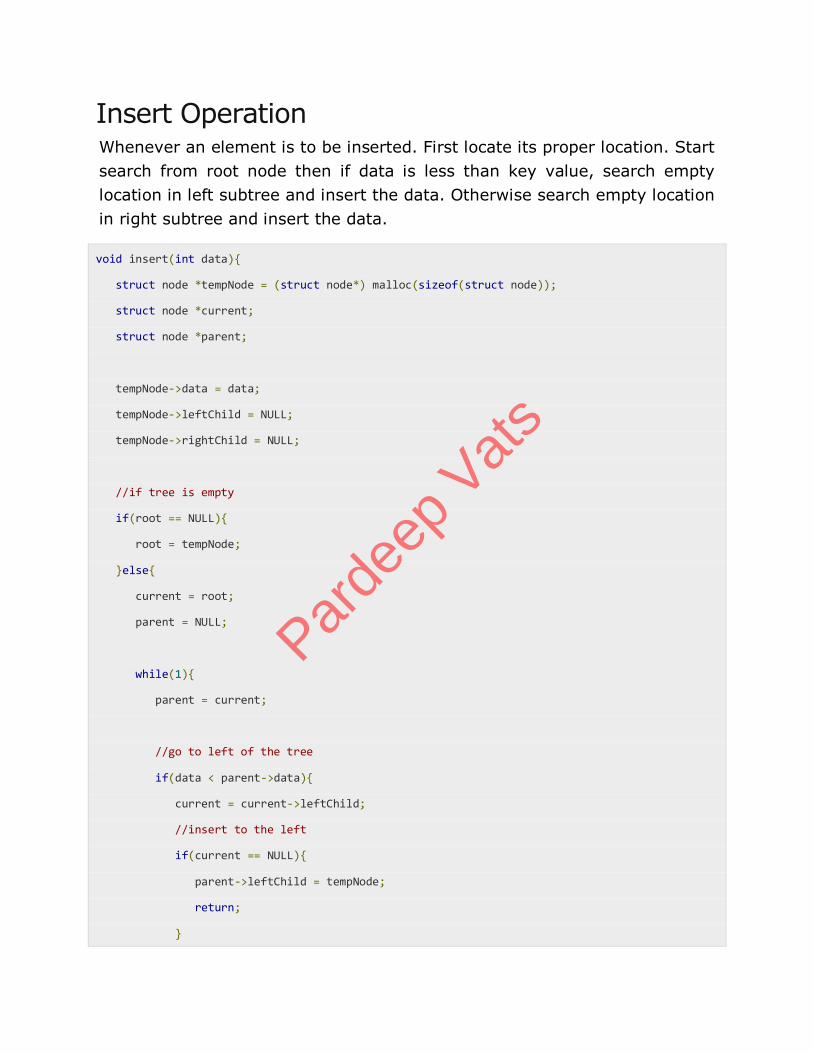
Insert Operation Whenever an element is to be inserted. First locate its proper location. Start
search from root node then if data is less than key value, search empty
location in left subtree and insert the data. Otherwise search empty location
in right subtree and insert the data.
void insert(int data){
struct node *tempNode = (struct node*) malloc(sizeof(struct node));
struct node *current;
struct node *parent;
tempNode->data = data;
tempNode->leftChild = NULL;
tempNode->rightChild = NULL;
//if tree is empty
if(root == NULL){
root = tempNode;
}else{
current = root;
parent = NULL;
while(1){
parent = current;
//go to left of the tree
if(data < parent->data){
current = current->leftChild;
//insert to the left
if(current == NULL){
parent->leftChild = tempNode;
return;
}
Parde
ep V
ats
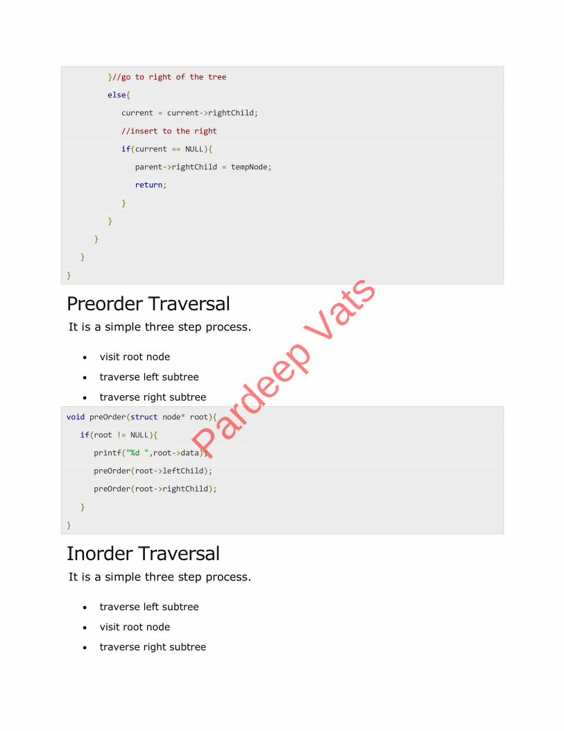
}//go to right of the tree
else{
current = current->rightChild;
//insert to the right
if(current == NULL){
parent->rightChild = tempNode;
return;
}
}
}
}
}
Preorder Traversal It is a simple three step process.
visit root node
traverse left subtree
traverse right subtree
void preOrder(struct node* root){
if(root != NULL){
printf("%d ",root->data);
preOrder(root->leftChild);
preOrder(root->rightChild);
}
}
Inorder Traversal It is a simple three step process.
traverse left subtree
visit root node
traverse right subtree
Parde
ep V
ats
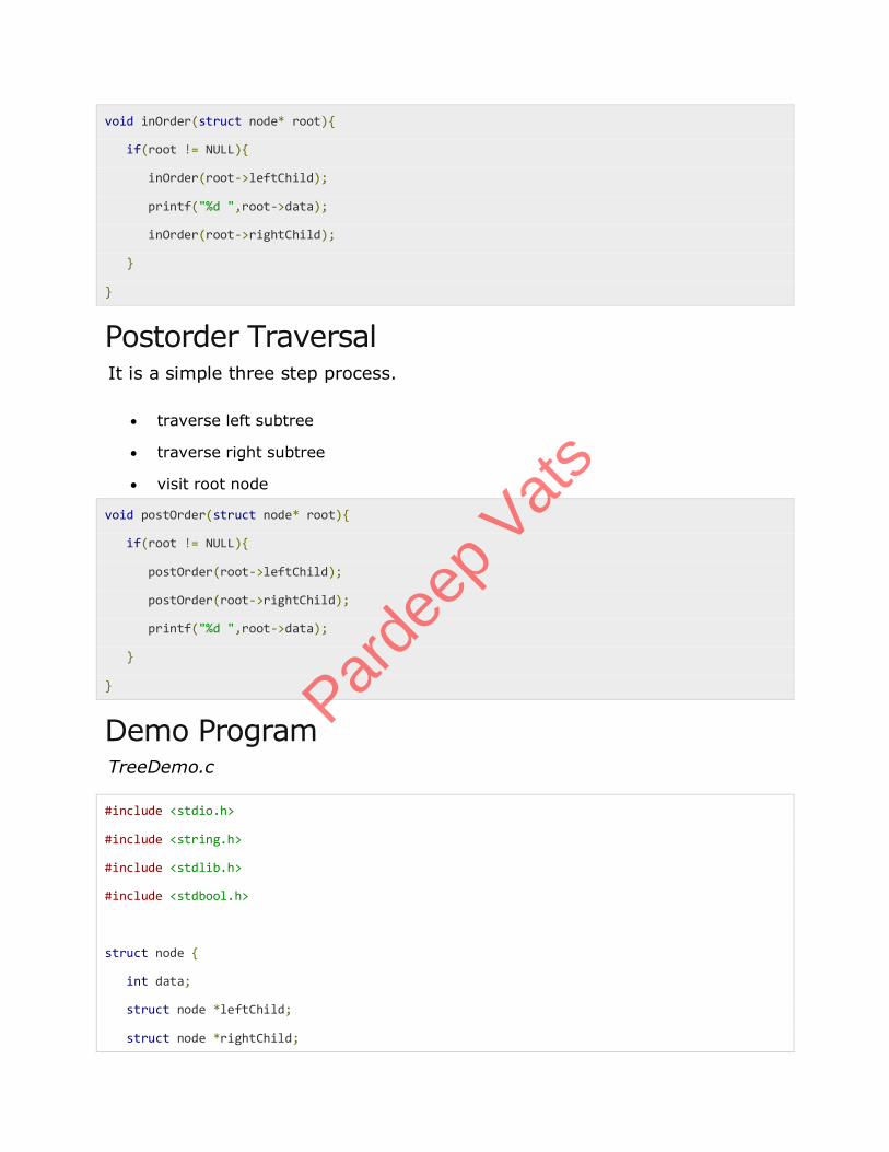
void inOrder(struct node* root){
if(root != NULL){
inOrder(root->leftChild);
printf("%d ",root->data);
inOrder(root->rightChild);
}
}
Postorder Traversal It is a simple three step process.
traverse left subtree
traverse right subtree
visit root node
void postOrder(struct node* root){
if(root != NULL){
postOrder(root->leftChild);
postOrder(root->rightChild);
printf("%d ",root->data);
}
}
Demo Program TreeDemo.c
#include <stdio.h>
#include <string.h>
#include <stdlib.h>
#include <stdbool.h>
struct node {
int data;
struct node *leftChild;
struct node *rightChild;
Parde
ep V
ats
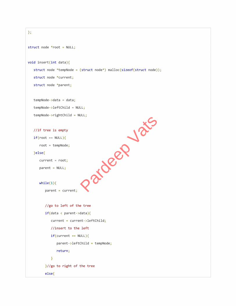
};
struct node *root = NULL;
void insert(int data){
struct node *tempNode = (struct node*) malloc(sizeof(struct node));
struct node *current;
struct node *parent;
tempNode->data = data;
tempNode->leftChild = NULL;
tempNode->rightChild = NULL;
//if tree is empty
if(root == NULL){
root = tempNode;
}else{
current = root;
parent = NULL;
while(1){
parent = current;
//go to left of the tree
if(data < parent->data){
current = current->leftChild;
//insert to the left
if(current == NULL){
parent->leftChild = tempNode;
return;
}
}//go to right of the tree
else{
Parde
ep V
ats
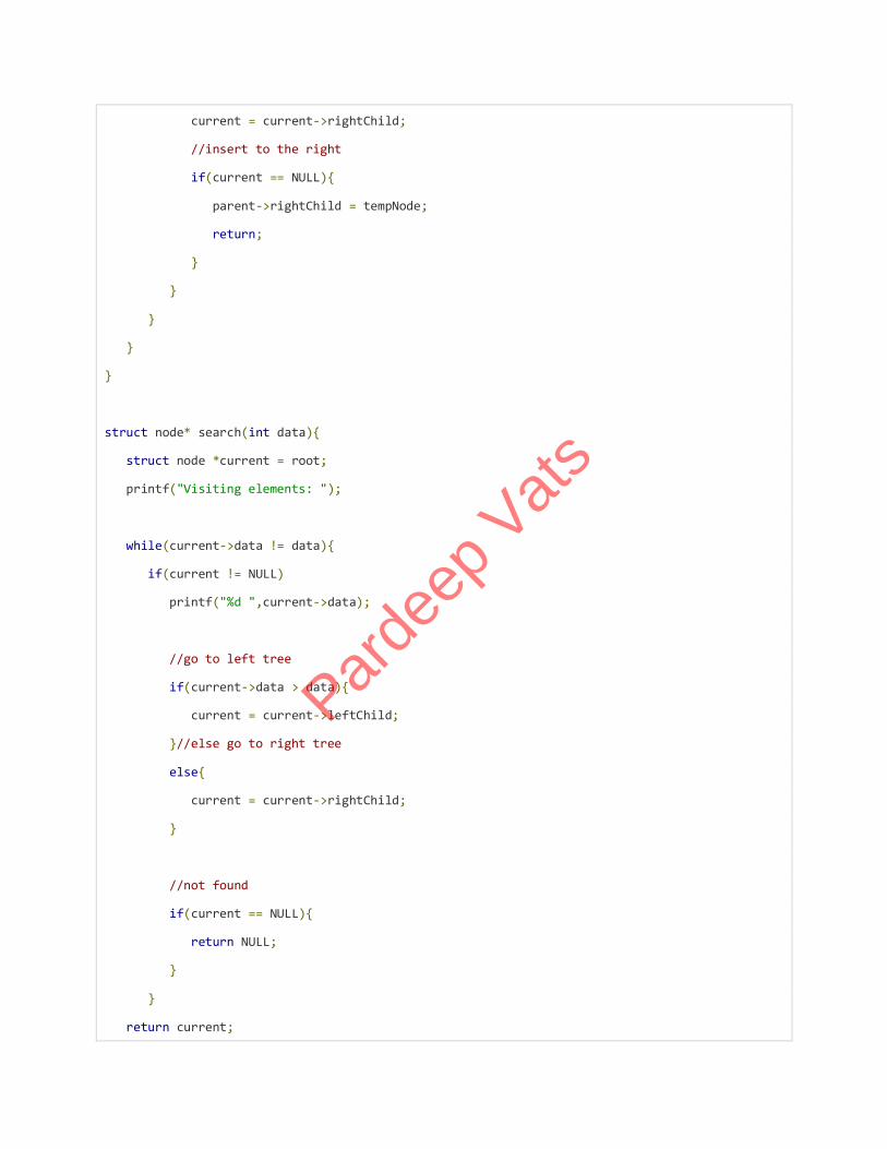
current = current->rightChild;
//insert to the right
if(current == NULL){
parent->rightChild = tempNode;
return;
}
}
}
}
}
struct node* search(int data){
struct node *current = root;
printf("Visiting elements: ");
while(current->data != data){
if(current != NULL)
printf("%d ",current->data);
//go to left tree
if(current->data > data){
current = current->leftChild;
}//else go to right tree
else{
current = current->rightChild;
}
//not found
if(current == NULL){
return NULL;
}
}
return current;
Parde
ep V
ats
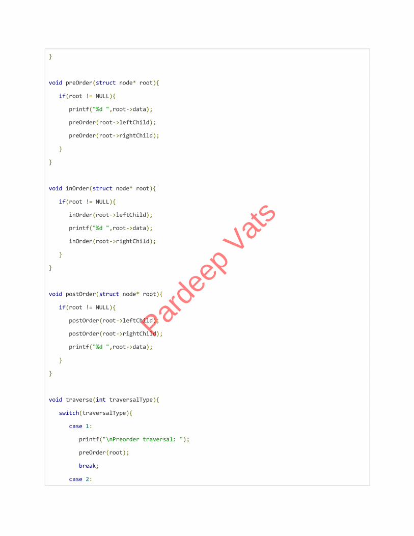
}
void preOrder(struct node* root){
if(root != NULL){
printf("%d ",root->data);
preOrder(root->leftChild);
preOrder(root->rightChild);
}
}
void inOrder(struct node* root){
if(root != NULL){
inOrder(root->leftChild);
printf("%d ",root->data);
inOrder(root->rightChild);
}
}
void postOrder(struct node* root){
if(root != NULL){
postOrder(root->leftChild);
postOrder(root->rightChild);
printf("%d ",root->data);
}
}
void traverse(int traversalType){
switch(traversalType){
case 1:
printf("\nPreorder traversal: ");
preOrder(root);
break;
case 2:
Parde
ep V
ats
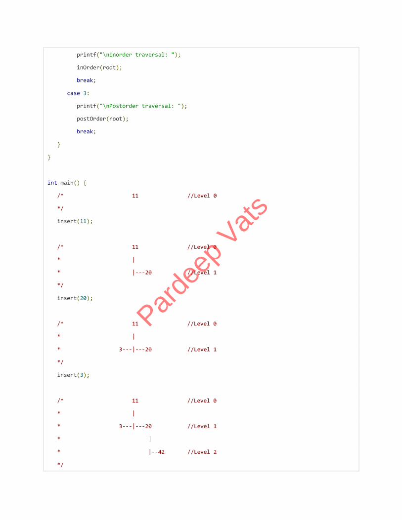
printf("\nInorder traversal: ");
inOrder(root);
break;
case 3:
printf("\nPostorder traversal: ");
postOrder(root);
break;
}
}
int main() {
/* 11 //Level 0
*/
insert(11);
/* 11 //Level 0
* |
* |---20 //Level 1
*/
insert(20);
/* 11 //Level 0
* |
* 3---|---20 //Level 1
*/
insert(3);
/* 11 //Level 0
* |
* 3---|---20 //Level 1
* |
* |--42 //Level 2
*/
Parde
ep V
ats
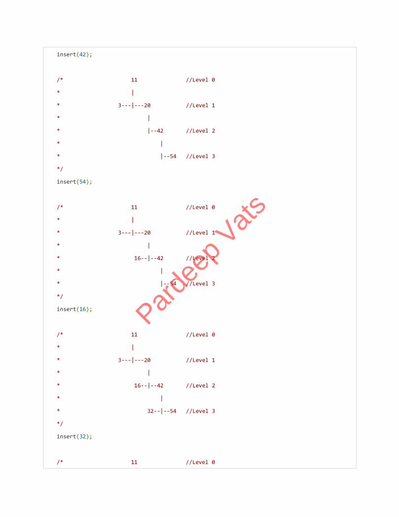
insert(42);
/* 11 //Level 0
* |
* 3---|---20 //Level 1
* |
* |--42 //Level 2
* |
* |--54 //Level 3
*/
insert(54);
/* 11 //Level 0
* |
* 3---|---20 //Level 1
* |
* 16--|--42 //Level 2
* |
* |--54 //Level 3
*/
insert(16);
/* 11 //Level 0
* |
* 3---|---20 //Level 1
* |
* 16--|--42 //Level 2
* |
* 32--|--54 //Level 3
*/
insert(32);
/* 11 //Level 0
Parde
ep V
ats
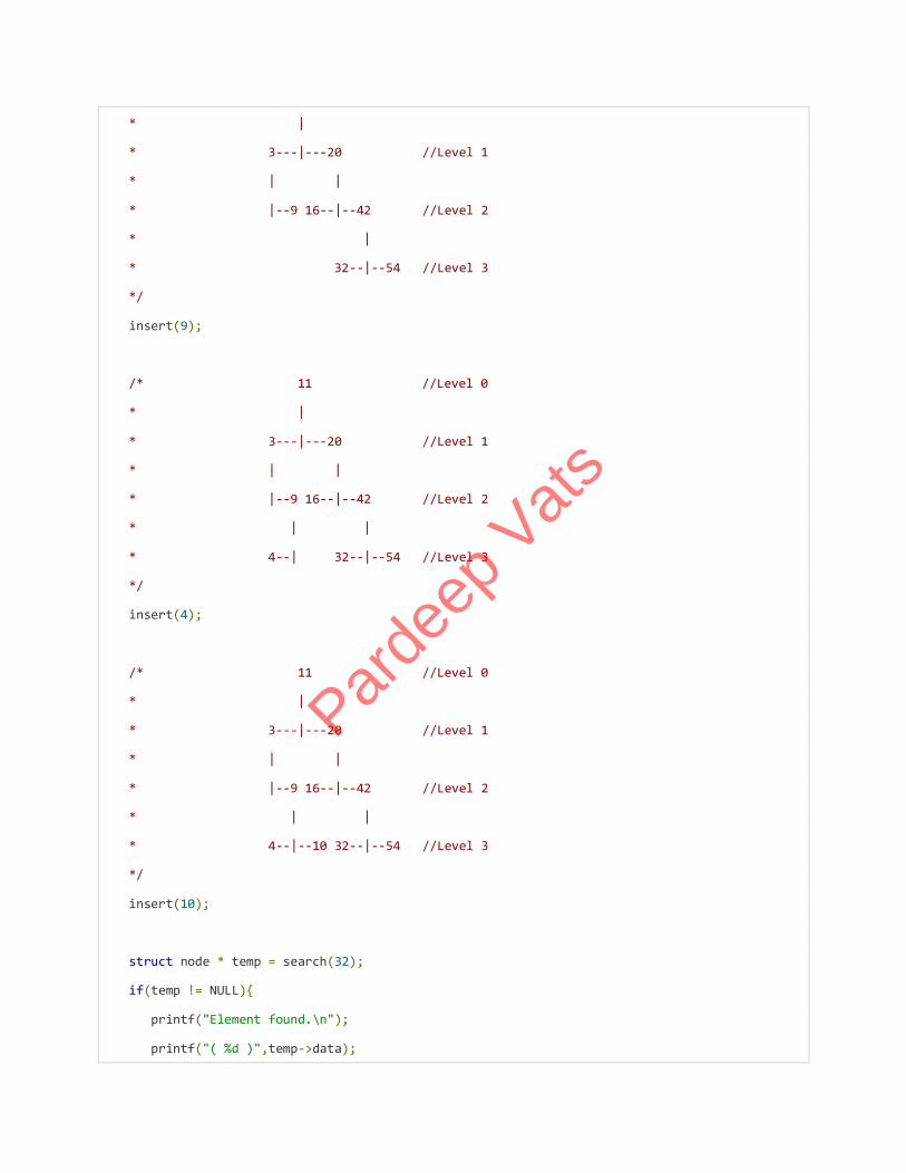
* |
* 3---|---20 //Level 1
* | |
* |--9 16--|--42 //Level 2
* |
* 32--|--54 //Level 3
*/
insert(9);
/* 11 //Level 0
* |
* 3---|---20 //Level 1
* | |
* |--9 16--|--42 //Level 2
* | |
* 4--| 32--|--54 //Level 3
*/
insert(4);
/* 11 //Level 0
* |
* 3---|---20 //Level 1
* | |
* |--9 16--|--42 //Level 2
* | |
* 4--|--10 32--|--54 //Level 3
*/
insert(10);
struct node * temp = search(32);
if(temp != NULL){
printf("Element found.\n");
printf("( %d )",temp->data);
Parde
ep V
ats
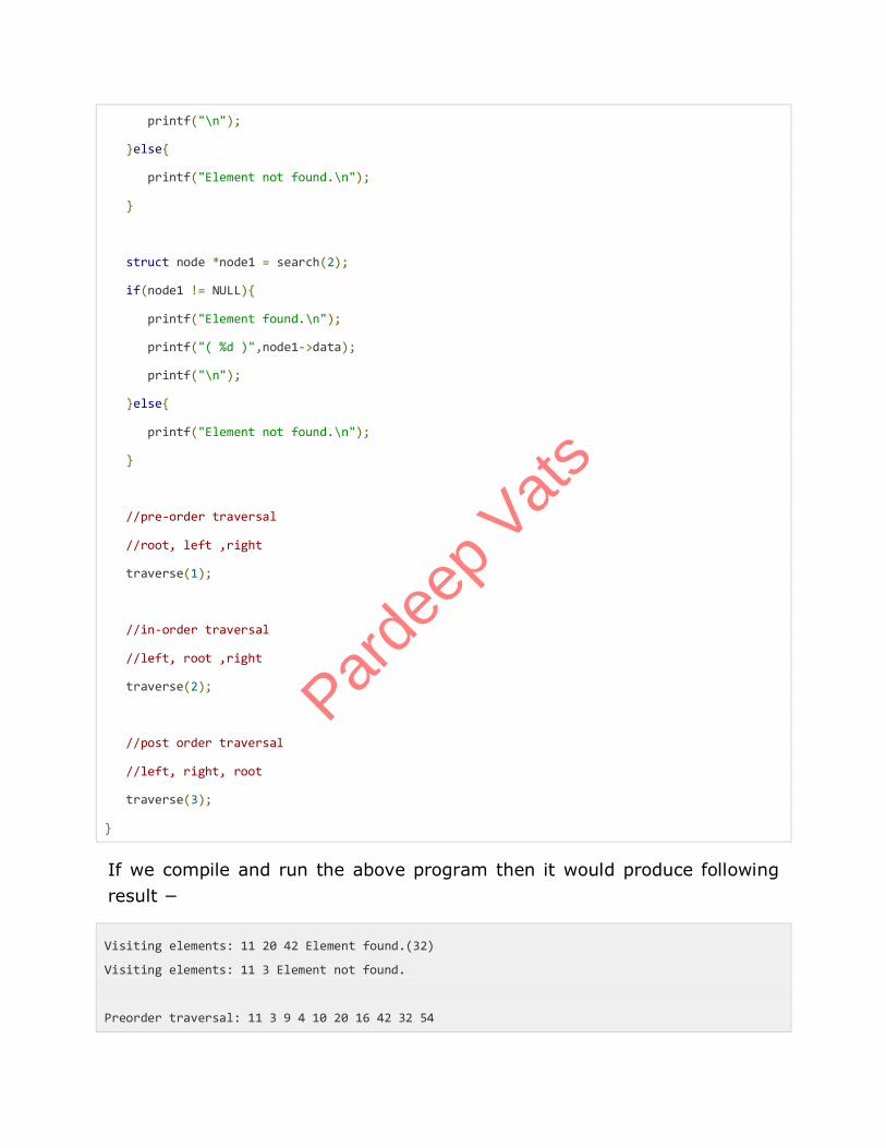
printf("\n");
}else{
printf("Element not found.\n");
}
struct node *node1 = search(2);
if(node1 != NULL){
printf("Element found.\n");
printf("( %d )",node1->data);
printf("\n");
}else{
printf("Element not found.\n");
}
//pre-order traversal
//root, left ,right
traverse(1);
//in-order traversal
//left, root ,right
traverse(2);
//post order traversal
//left, right, root
traverse(3);
}
If we compile and run the above program then it would produce following
result −
Visiting elements: 11 20 42 Element found.(32)
Visiting elements: 11 3 Element not found.
Preorder traversal: 11 3 9 4 10 20 16 42 32 54
Parde
ep V
ats
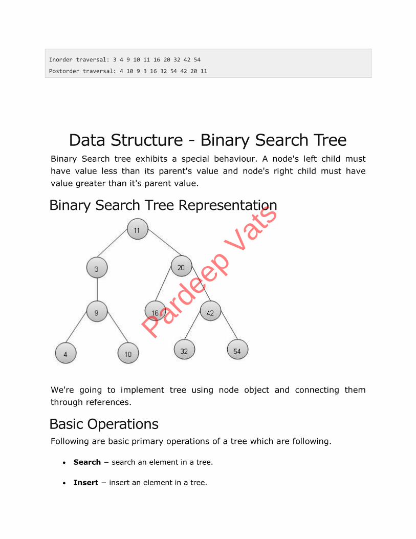
Inorder traversal: 3 4 9 10 11 16 20 32 42 54
Postorder traversal: 4 10 9 3 16 32 54 42 20 11
Data Structure - Binary Search Tree Binary Search tree exhibits a special behaviour. A node's left child must
have value less than its parent's value and node's right child must have
value greater than it's parent value.
Binary Search Tree Representation
We're going to implement tree using node object and connecting them
through references.
Basic Operations Following are basic primary operations of a tree which are following.
Search − search an element in a tree.
Insert − insert an element in a tree.
Parde
ep V
ats
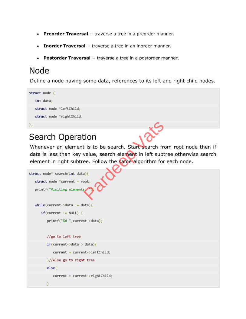
Preorder Traversal − traverse a tree in a preorder manner.
Inorder Traversal − traverse a tree in an inorder manner.
Postorder Traversal − traverse a tree in a postorder manner.
Node Define a node having some data, references to its left and right child nodes.
struct node {
int data;
struct node *leftChild;
struct node *rightChild;
};
Search Operation Whenever an element is to be search. Start search from root node then if
data is less than key value, search element in left subtree otherwise search
element in right subtree. Follow the same algorithm for each node.
struct node* search(int data){
struct node *current = root;
printf("Visiting elements: ");
while(current->data != data){
if(current != NULL) {
printf("%d ",current->data);
//go to left tree
if(current->data > data){
current = current->leftChild;
}//else go to right tree
else{
current = current->rightChild;
}
Parde
ep V
ats
//not found
if(current == NULL){
return NULL;
}
}
}
return current;
}
Insert Operation Whenever an element is to be inserted. First locate its proper location. Start
search from root node then if data is less than key value, search empty
location in left subtree and insert the data. Otherwise search empty location
in right subtree and insert the data.
void insert(int data){
struct node *tempNode = (struct node*) malloc(sizeof(struct node));
struct node *current;
struct node *parent;
tempNode->data = data;
tempNode->leftChild = NULL;
tempNode->rightChild = NULL;
//if tree is empty
if(root == NULL){
root = tempNode;
}else{
current = root;
parent = NULL;
while(1){
parent = current;
Parde
ep V
ats
//go to left of the tree
if(data < parent->data){
current = current->leftChild;
//insert to the left
if(current == NULL){
parent->leftChild = tempNode;
return;
}
}//go to right of the tree
else{
current = current->rightChild;
//insert to the right
if(current == NULL){
parent->rightChild = tempNode;
return;
}
}
}
}
}
Parde
ep V
ats
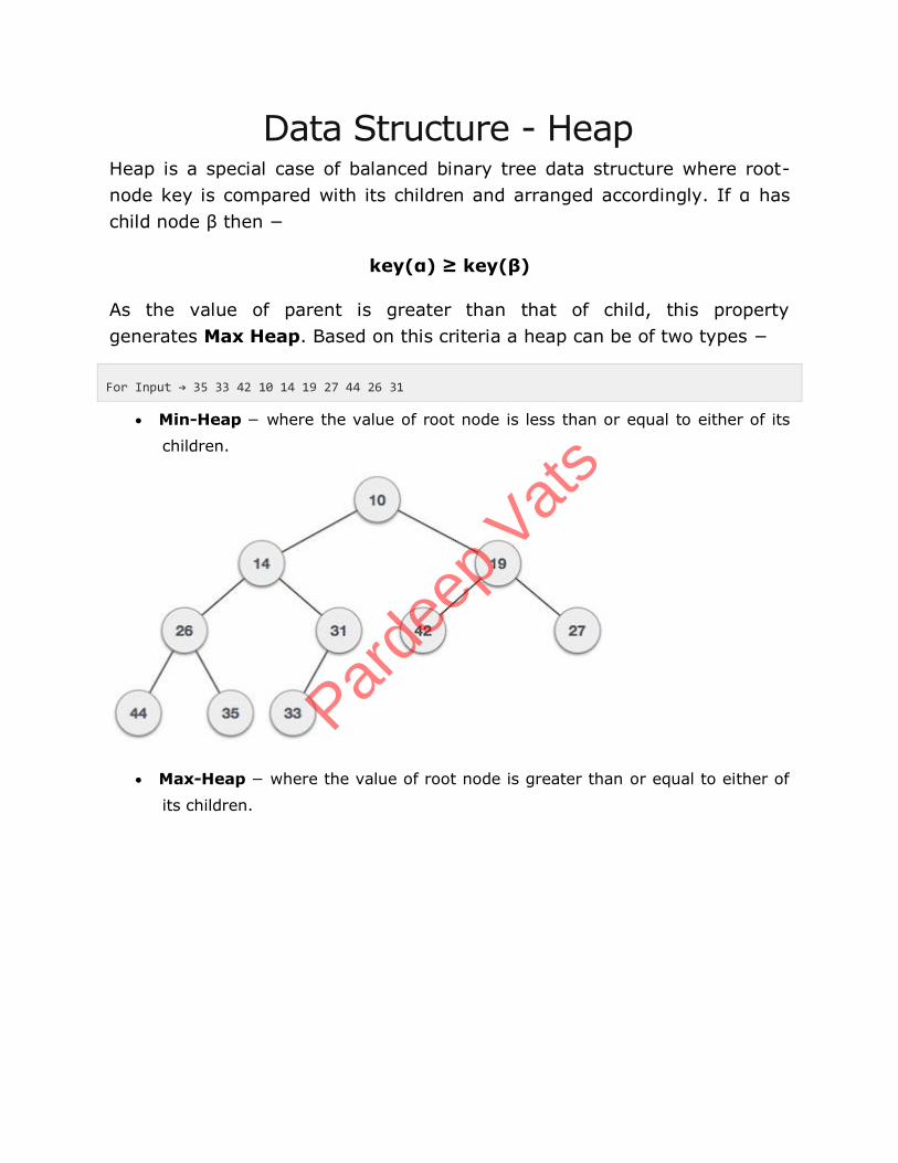
Data Structure - Heap Heap is a special case of balanced binary tree data structure where root-
node key is compared with its children and arranged accordingly. If α has
child node β then −
key(α) ≥ key(β)
As the value of parent is greater than that of child, this property
generates Max Heap. Based on this criteria a heap can be of two types −
For Input → 35 33 42 10 14 19 27 44 26 31
Min-Heap − where the value of root node is less than or equal to either of its
children.
Max-Heap − where the value of root node is greater than or equal to either of
its children.
Parde
ep V
ats
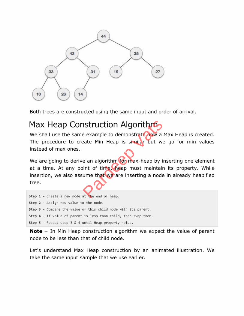
Both trees are constructed using the same input and order of arrival.
Max Heap Construction Algorithm We shall use the same example to demonstrate how a Max Heap is created.
The procedure to create Min Heap is similar but we go for min values
instead of max ones.
We are going to derive an algorithm for max-heap by inserting one element
at a time. At any point of time, heap must maintain its property. While
insertion, we also assume that we are inserting a node in already heapified
tree.
Step 1 − Create a new node at the end of heap.
Step 2 − Assign new value to the node.
Step 3 − Compare the value of this child node with its parent.
Step 4 − If value of parent is less than child, then swap them.
Step 5 − Repeat step 3 & 4 until Heap property holds.
Note − In Min Heap construction algorithm we expect the value of parent
node to be less than that of child node.
Let's understand Max Heap construction by an animated illustration. We
take the same input sample that we use earlier.
Parde
ep V
ats
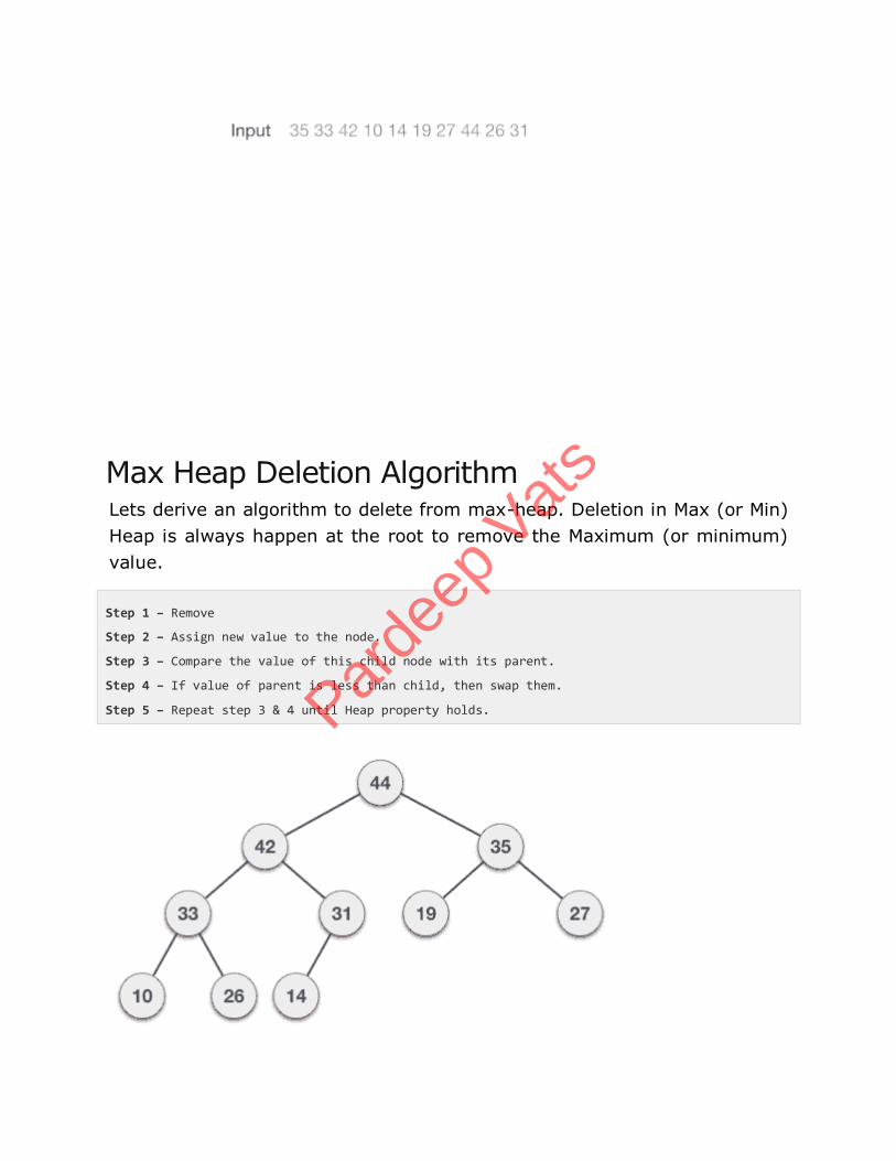
Max Heap Deletion Algorithm Lets derive an algorithm to delete from max-heap. Deletion in Max (or Min)
Heap is always happen at the root to remove the Maximum (or minimum)
value.
Step 1 − Remove
Step 2 − Assign new value to the node.
Step 3 − Compare the value of this child node with its parent.
Step 4 − If value of parent is less than child, then swap them.
Step 5 − Repeat step 3 & 4 until Heap property holds.
Parde
ep V
ats
Data Structure - Recursion Basics Some computer programming languages allows a module or function to call
itself. This technique is known as recursion. In recursion, a function α either
calls itself directly or calls a function β that in turn calls the original
function α. The function α is called recursive function.
Properties A recursive function can go infinite like a loop. To avoid infinite running of
recursive function, there are two properties that a recursive function must
have −
Base criteria − There must be at least one base criteria or condition, such that,
when this condition is met the function stops calling itself recursively.
Progressive approach − The recursive calls should progress in such a way
that each time a recursive call is made it comes closer to the base criteria.
Implementation Many programming languages implement recursion by means of stacks.
Generally, whenever a function (caller) calls another function (callee) or
itself as callee, the caller function transfers execution control to callee. This
transfer process may also involve some data to be passed from caller to
callee.
This implies, the caller function has to suspend its execution temporarily
and resume later when the execution control returns from callee function.
Here, caller function needs to start exactly from the point of execution
where it put itself on hold. It also needs the exact same data values it was
working on. For this purpose an activation record (or stack frame) is
created for caller function.
Parde
ep V
ats
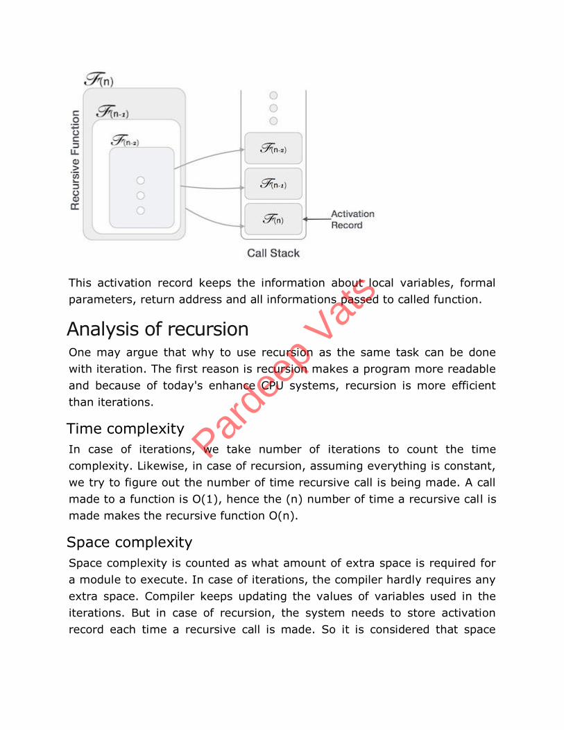
This activation record keeps the information about local variables, formal
parameters, return address and all informations passed to called function.
Analysis of recursion One may argue that why to use recursion as the same task can be done
with iteration. The first reason is recursion makes a program more readable
and because of today's enhance CPU systems, recursion is more efficient
than iterations.
Time complexity
In case of iterations, we take number of iterations to count the time
complexity. Likewise, in case of recursion, assuming everything is constant,
we try to figure out the number of time recursive call is being made. A call
made to a function is Ο(1), hence the (n) number of time a recursive call is
made makes the recursive function Ο(n).
Space complexity
Space complexity is counted as what amount of extra space is required for
a module to execute. In case of iterations, the compiler hardly requires any
extra space. Compiler keeps updating the values of variables used in the
iterations. But in case of recursion, the system needs to store activation
record each time a recursive call is made. So it is considered that space
Parde
ep V
ats
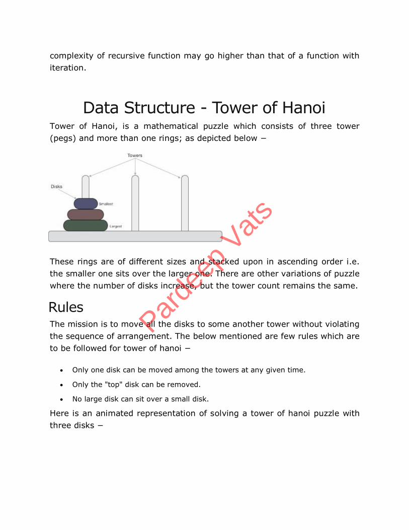
complexity of recursive function may go higher than that of a function with
iteration.
Data Structure - Tower of Hanoi Tower of Hanoi, is a mathematical puzzle which consists of three tower
(pegs) and more than one rings; as depicted below −
These rings are of different sizes and stacked upon in ascending order i.e.
the smaller one sits over the larger one. There are other variations of puzzle
where the number of disks increase, but the tower count remains the same.
Rules The mission is to move all the disks to some another tower without violating
the sequence of arrangement. The below mentioned are few rules which are
to be followed for tower of hanoi −
Only one disk can be moved among the towers at any given time.
Only the "top" disk can be removed.
No large disk can sit over a small disk.
Here is an animated representation of solving a tower of hanoi puzzle with
three disks −
Parde
ep V
ats
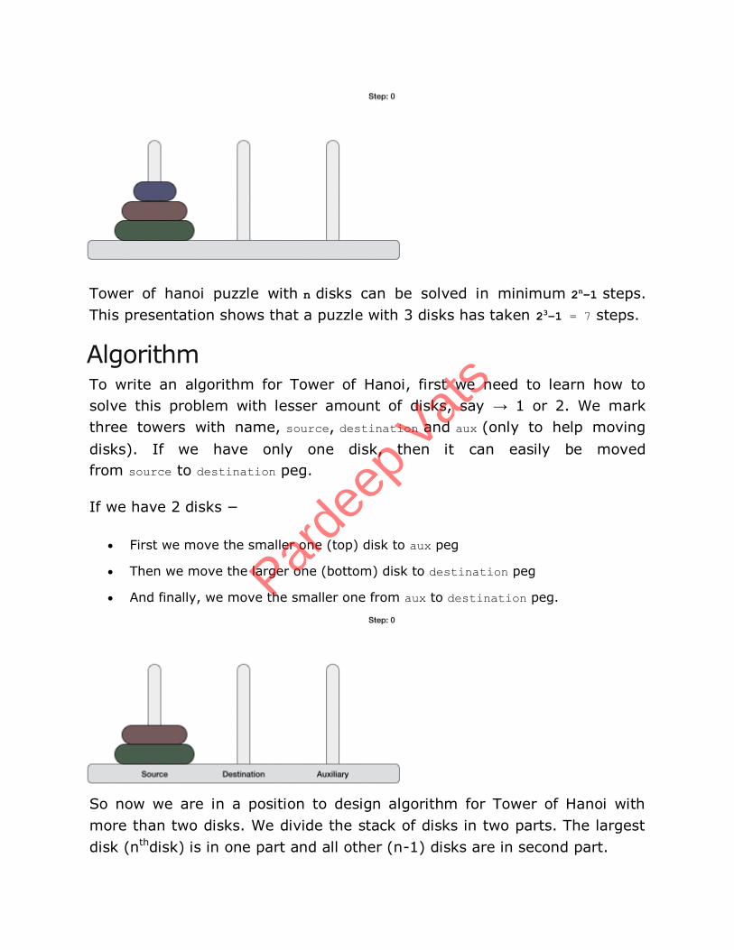
Tower of hanoi puzzle with n disks can be solved in minimum 2n−1 steps.
This presentation shows that a puzzle with 3 disks has taken 23−1 = 7 steps.
Algorithm To write an algorithm for Tower of Hanoi, first we need to learn how to
solve this problem with lesser amount of disks, say → 1 or 2. We mark
three towers with name, source, destination and aux (only to help moving
disks). If we have only one disk, then it can easily be moved
from source to destination peg.
If we have 2 disks −
First we move the smaller one (top) disk to aux peg
Then we move the larger one (bottom) disk to destination peg
And finally, we move the smaller one from aux to destination peg.
So now we are in a position to design algorithm for Tower of Hanoi with
more than two disks. We divide the stack of disks in two parts. The largest
disk (nthdisk) is in one part and all other (n-1) disks are in second part.
Parde
ep V
ats
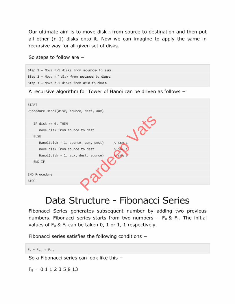
Our ultimate aim is to move disk n from source to destination and then put
all other (n-1) disks onto it. Now we can imagine to apply the same in
recursive way for all given set of disks.
So steps to follow are −
Step 1 − Move n-1 disks from source to aux
Step 2 − Move nth disk from source to dest
Step 3 − Move n-1 disks from aux to dest
A recursive algorithm for Tower of Hanoi can be driven as follows −
START
Procedure Hanoi(disk, source, dest, aux)
IF disk == 0, THEN
move disk from source to dest
ELSE
Hanoi(disk - 1, source, aux, dest) // Step 1
move disk from source to dest // Step 2
Hanoi(disk - 1, aux, dest, source) // Step 3
END IF
END Procedure
STOP
Data Structure - Fibonacci Series Fibonacci Series generates subsequent number by adding two previous
numbers. Fibonacci series starts from two numbers − F0 & F1. The initial
values of F0 & F1 can be taken 0, 1 or 1, 1 respectively.
Fibonacci series satisfies the following conditions −
Fn = Fn-1 + Fn-2
So a Fibonacci series can look like this −
F8 = 0 1 1 2 3 5 8 13
Parde
ep V
ats
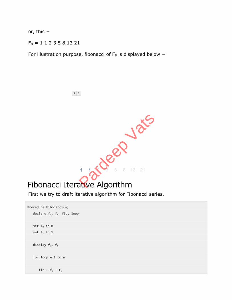
or, this −
F8 = 1 1 2 3 5 8 13 21
For illustration purpose, fibonacci of F8 is displayed below −
Fibonacci Iterative Algorithm First we try to draft iterative algorithm for Fibonacci series.
Procedure Fibonacci(n)
declare f0, f1, fib, loop
set f0 to 0
set f1 to 1
display f0, f1
for loop ← 1 to n
fib ← f0 + f1
Parde
ep V
ats
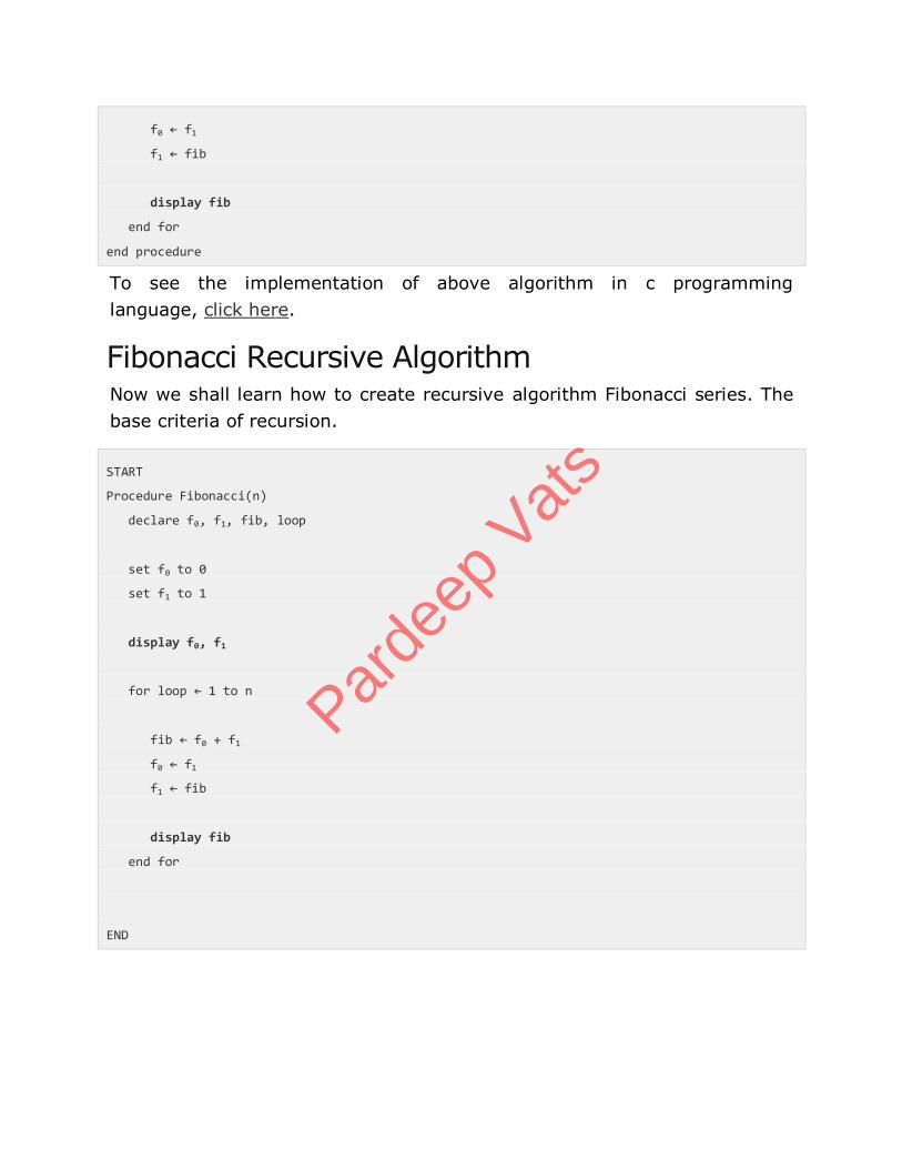
f0 ← f1
f1 ← fib
display fib
end for
end procedure
To see the implementation of above algorithm in c programming
language, click here.
Fibonacci Recursive Algorithm Now we shall learn how to create recursive algorithm Fibonacci series. The
base criteria of recursion.
START
Procedure Fibonacci(n)
declare f0, f1, fib, loop
set f0 to 0
set f1 to 1
display f0, f1
for loop ← 1 to n
fib ← f0 + f1
f0 ← f1
f1 ← fib
display fib
end for
END
Parde
ep V
ats