Embed Size (px)
Citation preview

DATA REQUIREMENTS RULE
AIR QUALITY CHARACTERIZATIONS
AND
“ROUND III” SO2 AREA DESIGNATION
RECOMMENDATIONS
AQPSTR 17-01
Illinois Environmental Protection Agency
Bureau of Air
1021 North Grand Avenue, East
Springfield, Illinois 62794-9276
January 12, 2017

Table of Contents
List of Tables 1
List of Figures 2
Executive Summary 4
1.0 Introduction/Background 5
2.0 Facility Selection 7
3.0 Air Quality Characterization: Dispersion Modeling 8
3.1 General Modeling Methodology 8
3.1.1 Modeling Domains and Emission Source Inventories 8
3.1.2 Terrain Processing (AERMAP) 10
3.1.3 Meteorological Data (AERSURFACE/AERMINUTE/AERMET) 10
3.1.3.1 Meteorological Data Selection 10
3.1.3.2 Meteorological Data Preprocessing 11
3.1.4 Model Implementation (AERMOD) 13
3.1.4.1 Dispersion Environment (Rural/Urban Determination) 13
3.1.4.2 Monitored Background 15
3.1.4.3 Model Execution and Output Evaluation 16
3.2 Facility-Specific Modeling Assessments 17
3.2.1 Kincaid Generation LLC 17
3.2.1.1 Modeling Domain and Receptor Network 17
3.2.1.2 Auer’s Analysis (Urban/Rural Environment) 19
3.2.1.3 Emissions 21
3.2.1.4 Meteorology 22
3.2.1.5 Background SO2 23
3.2.1.6 Modeling Results 24
3.2.2 Rain CII Carbon LLC 26
3.2.2.1 Modeling Domain and Receptor Network 27
3.2.2.2 Auer’s Analysis (Urban/Rural Environment) 28
3.2.2.3 Emissions 30

3.2.2.4 Meteorology 32
3.2.2.5 Background SO2 34
3.2.2.6 Modeling Results 34
3.2.3 Midwest Generation LLC – Waukegan 36
3.2.3.1 Modeling Domain and Receptor Network 36
3.2.3.2 Auer’s Analysis (Urban/Rural Environment) 38
3.2.3.3 Emissions 40
3.2.3.4 Meteorology 41
3.2.3.5 Background SO2 43
3.2.3.6 Modeling Results 43
3.2.4 Dynegy Midwest Generation – Baldwin/Prairie State Generating Station 45
3.2.4.1 Modeling Domain and Receptor Network 45
3.2.4.2 Auer’s Analysis (Urban/Rural Environment) 47
3.2.4.3 Emissions 51
3.2.4.4 Meteorology 52
3.2.4.5 Background SO2 53
3.2.4.6 Modeling Results 54
4.0 Air Quality Characterization: Ambient Monitoring 56
5.0 Area Designation Recommendations 58
Appendices 61
Appendix A 62
Appendix B 71

1
List of Tables
Table 1 Auer’s Land Use Classification Scheme 14
Table 2 Land Cover Mapping from NLCD to Auer’s Classifications 15
Table 3 Land Cover Percentages by Auer’s Category for a Three-Kilometer Radius Area and
for the Modeling Domain (45-Kilometer Radius) – Kincaid Study Area 20
Table 4 Facility Actual Emissions – Kincaid Study Area 22
Table 5 Maximum Predicted 99th
Percentile 1-Hour SO2 Design Value Concentration – Kincaid
Study Area 24
Table 6 Land Cover Percentages by Auer’s Category for a Three-Kilometer Radius Area and
for the Modeling Domain (25-Kilometer Radius) – Rain CII Carbon Study Area 30
Table 7 Facility Actual Emissions – Rain CII Carbon Study Area 31
Table 8 Maximum Predicted 99th
Percentile 1-Hour SO2 Design Value Concentration – Rain CII
Carbon Study Area 34
Table 9 Land Cover Percentages by Auer’s Category for a Three-Kilometer Radius Area and
for the Modeling Domain (30-Kilometer Radius) – Waukegan Study Area 39
Table 10 Facility Actual Emissions – Waukegan Study Area 40
Table 11 Maximum Predicted 99th
Percentile 1-Hour SO2 Design Value Concentration – Waukegan
Study Area 43
Table 12 Land Cover Percentages by Auer’s Category for 3-Kilometer Radius Areas – Baldwin
and Prairie State Generating Station 49
Table 13 Land Cover Percentages by Auer’s Category for the Modeling Domain (50-Kilometer
Radius) – Baldwin and Prairie State Generating Study Area 50
Table 14 Facility Actual Emissions – Baldwin and Prairie State Generating Study Area 52
Table 15 Maximum Predicted 99th
Percentile 1-Hour SO2 Design Value Concentration – Baldwin
and Prairie State Generating Study Area 54
Table 16 Summary of the Four Study Areas Maximum Predicted 99th Percentile 1-Hour SO2 Design
Value Concentration 59

2
List of Figures
Figure 1 Statewide Map Showing Locations of DRR – Listed Facilities 6
Figure 2 Kincaid Generation Study Area 17
Figure 3 Receptor Grid - Kincaid Study Area 18
Figure 4 Land Cover in the Kincaid Study Area (Urban vs. Rural) 19
Figure 5 Land Cover within a Three Kilometer Radius of Kincaid Generation
(Urban vs. Rural) 20
Figure 6 Abraham Lincoln Capital Airport Cumulative Annual Wind Rose 2013-2015 23
Figure 7 Maximum Predicted 99th
Percentile 1-Hour SO2 Concentrations – Kincaid Study Area
25
Figure 8 Rain CII Carbon Study Area 26
Figure 9 Receptor Grid – Rain CII Carbon Study Area 28
Figure 10 Land Cover in the Rain CII Carbon Study Area (Urban vs. Rural) 29
Figure 11 Land Cover within a Three-Kilometer Radius of Rain CII Carbon (Urban vs. Rural) 29
Figure 12 Evansville Regional Airport, Indiana, Cumulative Annual Wind Rose 2013-2015 33
Figure 13 Maximum Predicted 99th
Percentile 1-Hour SO2 Concentrations – Rain CII Carbon
Study Area 35
Figure 14 Midwest Generation LLC – Waukegan Study Area 36
Figure 15 Receptor Grid - Waukegan Study Area 37
Figure 16 Land Cover in the Waukegan Study Area (Urban vs. Rural) 38
Figure 17 Land Cover within a Three-Kilometer Radius of Waukegan Station (Urban vs. Rural) 39
Figure 18 Waukegan National Airport, Waukegan, Illinois Cumulative Annual Wind Rose 2013-
2015 42
Figure 19 Maximum Predicted 99th
Percentile 1-Hour SO2 Concentrations – Waukegan Study Area
44
Figure 20 Baldwin and Prairie State Generating Study Area 46
Figure 21 Receptor Grid – Baldwin and Prairie State Generating Station Study Area 47
Figure 22 Land Cover within a Three-Kilometer Radius of the Baldwin Plant (Urban vs. Rural) 48
Figure 23 Land Cover within a Three-Kilometer Radius of Prairie State Generating Station
(Urban vs. Rural) 49
Figure 24 Land Cover in the Baldwin and Prairie State Generating Study Area
(Urban vs. Rural) 50

3
Figure 25 Lambert – St. Louis International Airport, Missouri, Cumulative Annual Wind Rose
2013-2015 53
Figure 26 Maximum Predicted 99th
Percentile 1-Hour SO2 Concentrations – Baldwin and Prairie
State Generating Station Study Area 57
Figure 27 ADM SO2 and Meteorological Monitoring Location 57
Figure 28 Tate & Lyle Off-Property Northwest SO2 Monitoring Location 57
Figure 29 Tate & Lyle Southeast Fenceline SO2 Monitoring Location 58
4
Executive Summary
The U.S. Environmental Protection Agency (“USEPA”) has promulgated the Data Requirements
Rule (“DRR”)1 to support the final phases of implementation of the primary 1-hour sulfur dioxide
(“SO2”) National Ambient Air Quality Standard (“NAAQS”). This rulemaking requires regulatory
authorities to conduct air quality characterizations (through modeling or monitoring) of facilities with
annual emissions meeting or exceeding 2,000 tons (based upon the most recent year of available data)
or, alternatively, establishing federally enforceable source emission requirements that will limit a
facility’s emissions to a level below this threshold.
The Illinois Environmental Protection Agency (“Illinois EPA”) has conducted dispersion modeling to
characterize air quality around five facilities – Kincaid Generation (Kincaid, IL), Rain CII Carbon
(Robinson, IL), Midwest Generation (Waukegan, IL), Dynegy Midwest Generation (Baldwin, IL),
Prairie State Generating Company (Lively Grove, IL) – and is continuing to conduct modeling to
characterize air quality in the additional area around U.S. Steel Corporation (Granite City, IL) and
Gateway Energy & Coke Company (Granite City, IL). The Illinois EPA will also provide Primary
Quality Assurance Organization oversight responsibilities for an ambient monitoring program
operated by two other facilities – Archer Daniels Midland Company (Decatur, IL) and Tate & Lyle
Ingredients Americas (Decatur, IL) – which have been included in the Illinois EPA’s 2017
Monitoring Plan. The procedures and results described in this document are provided to USEPA in
fulfillment of Illinois EPA’s obligations under the DRR. Based upon the DRR dispersion modeling
results, the Illinois EPA is recommending designations of attainment of the 1-hour SO2 NAAQS for
the areas surrounding all facilities for which modeling has been completed. For the U.S.
Steel/Gateway Energy study area in Madison County, the Illinois EPA is currently providing an area
designation recommendation of unclassifiable pending resolution of uncertainties associated with
model inputs.
1 Data Requirements Rule for the 2010 1-Hour Sulfur Dioxide (SO2) Primary National Ambient Air Quality Standard
(NAAQS); Final Rule, Federal Register, Vol. 80, No. 162, August 21, 2015, p. 51052-51088.

5
1.0 Introduction/Background
The 1-hour SO2 NAAQS implementation process is on a court-approved schedule2 for completion of
area designations by USEPA in three rounds: the first round, which is now completed, was due by
July 2, 2016; the second round is due by December 31, 2017; and the final round is due by December
31, 2020. In the court-approved agreement containing that schedule, USEPA indicated that it would
designate two additional groups of areas by the July 2, 2016, deadline. These include areas that had
newly monitored violations of the NAAQS and areas “that contain any stationary source that
according to the EPA’s Air Markets Database either emitted more than 16,000 tons of SO2 in 2012 or
emitted more than 2,600 tons of SO2 and had an emission rate of at least 0.45 pounds SO2/mmbtu in
2012 that has not been announced (as of March 2, 2015) for retirement.”3 Illinois had five facilities
that met the criteria established in the court order – Hennepin Power Station (Putnam County),
Newton Power Station (Jasper County), Joppa Steam Coal Power Plant (Massac County), Marion
Power Station (Williamson County), and the Wood River Power Station (Madison County). USEPA
has finalized the area designations for these five facilities under the first round of the schedule.
The final implementation phases of the 1-hour SO2 NAAQS incorporate the December 31, 2017, and
December 31, 2020, deadlines agreed to in the March 2, 2015, court order and the closely-linked
requirements specified in the DRR. The DRR directs air regulatory authorities to characterize current
air quality around sources that emitted greater than 2,000 tons per year (“tpy”) in the most recent year
for which data was available. Based upon the criteria and conditions set forth in the rule, the Illinois
EPA has characterized air quality around five facilities using dispersion modeling – Kincaid
Generation (Kincaid, IL), Rain CII Carbon (Robinson, IL), Midwest Generation (Waukegan, IL),
Dynegy Midwest Generation (Baldwin, IL), and Prairie State Generating Company (Lively Grove,
IL). The Illinois EPA is also continuing to conduct modeling to characterize air quality in the area
around the “single source” consisting of U.S. Steel Corporation and Gateway Energy & Coke
Company (Granite City, IL). As the modeling in this area is still ongoing due to uncertainties
associated with model inputs, the area is not further addressed in this document. For two additional
facilities – Archer Daniels Midland Company (Decatur, IL) and Tate & Lyle Ingredients Americas
(Decatur, IL) – air quality will be characterized through ambient monitoring that commenced prior to
January 1, 2017, and will continue for at least three years.
These facilities are a subset of those that were required to be identified to USEPA in January 2016.4
The locations of these facilities are shown on the map provided in Figure 1. Thus, the air quality
characterization of DRR facilities, through monitoring and modeling as identified in this document,
will inform and facilitate the area designations process for the second and third rounds of the
schedule (March 2, 2015, court order, Sierra Club v. McCarthy). The Illinois EPA was required to
2 Sierra Club v. McCarthy, No. 3-13-cv-3953 (SI) (N.D. Cal. Mar. 2, 2015).
3 March 20, 2015, Memorandum from Janet G. McCabe, Acting Assistant Administrator (USEPA) to Lisa Bonnett, Director, Illinois
Environmental Protection Agency. 4 January 12, 2016, letter to Dr. Susan Hedman, Regional Administrator, USEPA Region V, from Lisa Bonnett, Director, Illinois
Environmental Protection Agency.

6
submit a modeling protocol5 (“Protocol”) to U.S. EPA by July 1, 2016, for each facility to be
modeled under the DRR. That protocol, together with comments received from U.S. EPA regarding
the protocol, were followed in the analyses performed. By that same date required for protocol
submission, the Illinois EPA provided information in its annual monitoring plan on planned monitors
at those facilities that will be characterized through ambient monitoring under the DRR.
Figure 1
Statewide Map Showing Locations of DRR - Listed Facilities
5 Sulfur Dioxide Air Quality Characterization Protocol: Facilities Warranting Evaluation Under the Data Requirements
Rule, AQPSTR 16-08, Illinois Environmental Protection Agency, June 30, 2016.
7
2.0 Facility Selection
Based upon company-reported actual SO2 emissions for calendar year 2014, which was the most
recent year of certified emissions data available to the Illinois EPA at the time of DRR facility
notification to USEPA in January 2016, 15 facilities which exceeded the emissions threshold of 2,000
tons per year were identified for inclusion in the air quality characterization process. As identified
earlier, the U.S. Steel Corporation – Granite City Works and Gateway Energy & Coke Company LLC
facilities (“U.S. Steel Study Area”) are regarded as a “single source” under Clean Air Act Title V
permitting, and collectively reported emissions that exceeded the threshold. On January 12, 2016, the
Illinois EPA submitted to USEPA Region V a list of facilities for SO2 air quality characterization, as
required under the DRR. It is noteworthy that the DRR stipulates the following: “due to the overlap
between the criteria for inclusion of sources in this final rule and those in the March 2015 consent
decree, all of the sources identified in the March 2015 consent decree should also be included on the
January 2016 list of sources required for characterization under this rule.” Thus, the DRR list
includes the five electrical generating stations that were modeled under Phase 2 (Illinois Power
Generating Company – Newton; Dynegy Midwest Generation LLC – Wood River; Electric Energy,
Inc. – Joppa; Dynegy Midwest Generation LLC – Hennepin; Southern Illinois Power Cooperative –
Marion), but which will not be further addressed in this document.
Additionally, the Midwest Generation LLC – Joliet electrical generating station was modeled in
conjunction with the Phase 1 Lemont nonattainment area analysis, though not part of the Lemont
nonattainment area. In the R15-21 rulemaking adopted by the Illinois Pollution Control Board and
submitted to USEPA as a State Implementation Plan (“SIP”) revision, the three units at this facility
cannot combust coal on and after December 31, 2016.6 The conversion from coal combustion to
natural gas combustion (with fuel oil backup in the event of natural gas curtailment) will reduce this
facility’s SO2 emissions to well below 2,000 tons per year, and thus obviate the need for additional air
quality characterization.
Lastly, the DTE Tuscola LLC facility (Tuscola, IL) also appeared on the DRR list because it had
reported SO2 emissions of 9,677 tons in 2014. This cogeneration facility has since ceased burning
coal in its boilers. In Illinois Construction Permit #15060039, the coal-firing capability of the three
boilers is permanently eliminated, as clearly stipulated in Condition 1.1.5 c: “Beginning January 30,
2016, natural gas, propane, and fuel gas . . . shall be the only fuels fired in the affected boilers.” As a
result of the reduced SO2 emissions, the DTE Tuscola LLC facility was not evaluated for air quality
despite appearing on the DRR list.
6 35 Illinois Administrative Code 225.296(b)

8
3.0 Air Quality Characterization: Dispersion Modeling
3.1 General Modeling Methodology
Dispersion modeling performed by the Illinois EPA conforms to regulatory procedures described in
The Guideline on Air Quality Models7 and recommended practices identified in the draft SO2 NAAQS
Designations Modeling Technical Assistance Document8 (“TAD”). The AERMOD modeling system
(which includes the AERMOD dispersion model, the AERMAP terrain preprocessor, and the
AERMINUTE and AERMET meteorological preprocessors) were used to simulate ambient impacts
from the DRR facilities. AERMOD is the preferred software for use in regulatory applications, and is
particularly suitable for this specific set of air quality analyses given the terrain, stack to structure
relationships, dispersion environment, and available meteorological data. AERMOD (version 15181)
was run exclusively in the regulatory default mode. The most recent three years (2013-2015) of
meteorological data determined to be representative of a facility’s airshed were used in combination
with surface characteristics data obtained from AERSURFACE (version 13016) for simulating the
area’s planetary boundary layer turbulence structure.
Illinois EPA staff prepared detailed site characterizations of each DRR facility to support
development of specific AERMOD inputs. Building-induced plume downwash was addressed for all
discretely modeled stacks and flares that were within the zone of influence of nearby buildings. The
Illinois EPA used USEPA’s Building Profile Input Program with PRIME algorithm (BPIPPRM,
dated 04274) to determine building parameters to model building wake effects. A relatively standard
approach to receptor network design, consisting of discrete fenceline receptors (spaced at
approximately 50-meter intervals) and a gridded receptor array extending outward to as much as 26
kilometers from the facility, was integral to each area-specific analysis.
3.1.1 Modeling Domains and Emission Source Inventories
Modeling domains were developed based upon the guidance provided in the draft modeling TAD and
the professional judgment of Illinois EPA modeling staff. These domains reflect the following
considerations: 1) the locations of the DRR-listed facility and potentially significant “near-field” SO2
emission sources, 2) stack heights, emission rates, and related plume release characteristics, 3) the
location and likely extent of significant concentration gradients of nearby sources, and 4) receptor
coverage and density that is sufficient to adequately capture and resolve model-predicted maximum
SO2 concentrations. The modeling domains represent the geographic extent of possible emission
source inclusion, and are circular constructs with radii ranging in size from 15-50 kilometers. These
domains are centered on the respective DRR facilities, with the exception of the combined domain
that includes the Dynegy Midwest Generation – Baldwin power plant and the Prairie State Generating
7 40 CFR Part 51, Appendix W.
8 SO2 NAAQS Designations Modeling Technical Assistance Document (draft), February 2016, USEPA
(OAR/OAQPS/AQAD), Research Triangle Park, NC.

9
Company power plant. Since areas of significant impact are not expected to occur at distances
representing the furthest extent of the modeling domains, all of the receptor networks are of smaller
geographic coverage than the full modeling domains.
The Illinois EPA had formally requested and received hourly-specific emission rates and stack
parameter data for 2012-2015 from both DRR and selected background facilities to best represent
ambient loadings in the study area and to obtain the best possible time-resolved estimates for
modeling years 2013-2015. Depending upon source and stack monitoring requirements, hourly-
specific data may not have been available for certain process sources. In the absence of such data,
estimates were derived from production information (including fuel usage/throughput quantities),
reported operational periods, stack test information, and/or other data sources.
The Illinois EPA has relied upon annual emission reports and other information in its Integrated
Comprehensive Environmental Management System (“ICEMAN”) statewide database to supplement
the information provided in response to the DRR data requests. Some data has been provided by
USEPA and the Indiana Department of Environmental Management (“IDEM”) in response to specific
requests.
Most sources modeled represent point sources, including flares, but for some of the facilities, selected
releases are represented as volume sources. Point source stack configurations are typically vertical
with unobstructed releases, but there are some stacks with “raincaps,” and other stacks that represent
horizontal releases. For the latter, each source’s exit velocity was adjusted in the manner
recommended in the AERMOD Implementation Guide.9 This guidance document specifically
indicates that the “user should input the actual stack diameter and exit temperature but set the exit
velocity to a nominally low value, such as 0.001 m/s.” Flares were modeled with adjusted release
parameters, consistent with current modeling guidance. The adjusted parameters include fixed values
for temperature (1273 degrees Kelvin) and exit velocity (20 meters/second) and modified values for
release height and diameter. The AERSCREEN User’s Guide10
provides the equation for calculating
the effective flare height:
Hsl = Hs + 4.56 x 10⁻³
(Hr/4.1868)0.478
where,
Hsl = effective flare height (meters)
Hs = stack height above ground (meters)
Hr = total heat release rate (Joules/second)
9 AERMOD Implementation Guide. 2009. U.S. Environmental Protection Agency, Research Triangle Park, NC.
10 AERSCREEN User’s Guide. EPA-454/B-11-001. U.S. Environmental Protection Agency, Research Triangle Park, NC.

10
The screening modeling documentation also provides the equation for calculating the effective
diameter for the flare:
D = 9.88 x 10⁻⁴
x [HR x (1-HL)]0.5
where,
D = effective stack diameter (meters)
HR = heat release rate (calories/second)
HL = heat loss fraction [used default value of 0.55]
3.1.2 Terrain Processing (AERMAP)
Procedures for selecting and processing terrain data are provided by the User’s Guide for the
AERMOD Terrain Preprocessor (AERMAP),11
and the March 2011 AERMAP User’s Guide
Addendum (version 11103).12
Selection of terrain data corresponds to the geographic areas represented by the modeling domains.
U.S. Geological Survey (“USGS”) National Elevation Dataset (“NED”) input data was used for all
DRR modeling. The latest NED data were obtained in TIFF format directly from the USGS for the
individual study areas. This data format is compatible for use with AERMAP. The final NED TIFF
files have a resolution of one arc second (30 meters) and the data is stored in a Geographic
(latitude/longitude) coordinate system based on the North American Datum of 1983 (“NAD83”).
Conversions from latitude/longitude to Universal Transverse Mercator (“UTM”) coordinates take
place within AERMAP using the UTMGEO program. NADCON conversion software (version 2.1)
is incorporated to calculate datum shifts, where necessary. AERMAP (version 11103) was run within
the BEEST for Windows software. Elevations from the NED data were determined for all sources
and structures, and both elevations and representative hill heights were determined for receptors.
This data was subsequently input to AERMOD.
3.1.3 Meteorological Data (AERSURFACE/AERMINUTE/AERMET)
3.1.3.1 Meteorological Data Selection
Procedures for selecting and developing meteorological data have been provided in the draft
document Regional Meteorological Data Processing Protocol, EPA Region 5 and States.13
Within
this document, content pertaining to selection criteria for surface meteorological data addresses the
representativeness of meteorological data collection sites to the emission source/receptor impact area.
11
User’s Guide for the AERMOD Terrain Preprocessor (AERMAP). EPA-454/B-03-003, October 2004. U.S.
Environmental Protection Agency, Research Triangle Park, NC. 12
Addendum – User’s Guide for the AERMOD Terrain Preprocessor (AERMAP). EPA-454/B-03-003 (October, 2004).
U.S. Environmental Protection Agency, Research Triangle Park, NC. 13
Draft – Regional Meteorological Data Processing Protocol. EPA Region 5 and States. August 2014.

11
There are two criteria to be considered: 1) the suitability of meteorological data for the study area,
and 2) the actual similarity of surface conditions and surroundings at the emission source/receptor
impact area compared to the location of the meteorological instrumentation tower. The closest
National Weather Service (“NWS”) surface meteorological data station was believed to be the most
acceptable for most modeling domains. Similarly, upper air data for processing with surface
meteorological data was chosen on the basis of regional representativeness.
3.1.3.2 Meteorological Data Preprocessing
Procedures for processing meteorological data are provided in the 2004 User’s Guide for the
AERMOD Meteorological Preprocessor (AERMET)14
and in the 2014 AERMET User’s Guide
Addendum.15
AERMET (version 15181) processes raw meteorological data to produce higher order
data that can be read by the AERMOD model. The first two stages of processing the raw data
involve QA/QC of the meteorological data and then correlating the surface data with upper air data.
While standard NWS surface data include meteorological data records recorded near the beginning of
each hour, additional wind speed and wind direction data recorded at one-minute intervals were also
included in the development of higher order meteorological data. Automated Surface Observing
System (“ASOS”) one-minute wind data obtained for NWS surface stations were processed using
AERMINUTE (version 15272), as specified in the companion AERMINUTE User’s Instructions.16,17
A third and final stage reads the merged surface and upper air data file and processes surface
characteristics data at the tower site for final generation of meteorological files to be read into the
AERMOD modeling runs.
The surface conditions data are provided through another preprocessor called AERSURFACE, and
processing was conducted consistent with documentation in the AERSURFACE User’s Guide.18
In
response to comments received from USEPA regarding the Illinois EPA’s modeling protocol
document, the Illinois EPA clarified that the AERSURFACE processing conducted for the DRR used
1992 land cover data and not 2011 National Land Cover Data. AERSURFACE is a tool using land
cover data around the meteorological tower site to principally determine surface roughness by wind
sector. A wind sector is defined by a wedge shaped area extending from the tower out to one
kilometer, but not exceeding 30 degrees in angular width. The total circular area had no more than 12
sectors. Two other parameters, Bowen ratio and albedo, are determined more on a regional basis, but
also based on land cover. All three factors can change with the seasons, as well as on a monthly
basis. Meteorological conditions vary from year to year, resulting in periods that can be abnormally
14
User’s Guide for the AERMOD Meteorological Preprocessor (AERMET). 2004. EPA-454/B-03-002. U.S.
Environmental Protection Agency, Research Triangle Park, NC. 15
Addendum – User’s Guide for the AERMOD Meteorological Preprocessor (AERMET). EPA-454/B-03-002
(November, 2014). U.S. Environmental Protection Agency, Research Triangle Park, NC. 16
AERMINUTE User’s Instructions (Draft). 2011. U.S. Environmental Protection Agency, Research Triangle Park, NC. 17
AERMINUTE User’s Instructions. 2014. U.S. Environmental Protection Agency, Research Triangle Park, NC. 18
Revised – AERSURFACE User’s Guide (Revised January 16, 2013). EPA-454/B-08-001 (January, 2008). U.S.
Environmental Protection Agency, Research Triangle Park, NC.

12
dry one year, and wet the following year, or simply exhibiting average conditions. In augmenting
Stage 3 parameters to accommodate monthly variability, the Illinois EPA has calculated values for
albedo, Bowen ratio, and surface roughness on a monthly basis in order to provide greater temporal
resolution in the characterization of surface moisture and in capturing the influence of snow cover.
Thus, AERSURFACE has been run in a monthly format for wet, dry, and average moisture
conditions for both snow cover and no snow cover.
Determinations regarding snow cover are based upon Local Climatological Data (“LCD”) from the
National Weather Service surface collecting station. The LCD indicates which individual days had
snow cover and the snow depth for that particular day. Days with greater than a trace amount of
snow are considered to have snow cover. The fraction of days per month with snow cover were
multiplied by the value for snow cover applicable to albedo and surface roughness values. This
approach was also implemented for values involving no snow cover. The computed values were
added and then divided by the number of days in a particular month. The end result was an averaged
value for each month for regional albedo and surface roughness by wind sector. These calculations
were produced through a spreadsheet, as are the ones described below.
With regard to moisture levels, the determination of a “wet” or “dry” recent year has been made
based upon what was known about precipitation records over historical periods of time that might
range over 50 or more years. Generally, an average for each month was calculated over 30 years of
data. A dry month is considered to be that month where the monthly total was at or below 0.6 times
the average. A wet month would be a month where the monthly total of precipitation would be at or
over 1.2 times the average. Months within 0.6 to 1.2 times the average precipitation were considered
to be normal or average. These ratios were determined from guidelines set forth in the
AERSURFACE User’s Guide. According to this document, a dry month can be considered to be that
month where the monthly precipitation total falls under the lower 30th percentile of monthly records.
A wet month can be a month where the monthly total of precipitation would be above the upper 30th
percentile of monthly records. An average month would fall in between the lower and upper 30th
percentiles. Months evaluated as being “dry” used the Bowen ratio that was determined for a “dry”
month from the AERSURFACE runs. Likewise, “wet” and “average” months determined from the
LCD data were linked to corresponding output in the AERSURFACE runs. For winter months, after
the evaluation of monthly moisture is made, the Bowen Ratio is additionally averaged for days of
snow cover in the same way as albedo.
In general, typical monthly values for albedo can be affected by the presence of snow but not by
moisture. Similarly, surface roughness can be influenced by snow, but not by moisture. Monthly
values for Bowen ratio can be influenced by snow cover and moisture.
Surface meteorological data used by AERMET were obtained from multiple sources. Hourly surface
meteorological data records are read by AERMET that include all the necessary elements for
meteorological data processing, including wind direction and wind speed. Wind data taken at hourly
intervals may not always portray wind conditions for the entire hour, which can be variable in nature

13
compared to more stable meteorological properties not susceptible to wide-ranging changes. Wind
data that portray calm conditions for particular hours are not usable for modeling purposes, and must
be passed over by AERMOD when modeling is being performed. In order to better represent actual
wind conditions at the meteorological tower, wind data of one-minute duration were obtained for the
same meteorological tower but in a different formatted meteorological file, and processed using
AERMINUTE. These data were subsequently integrated into the AERMET meteorological data
processing to produce final hourly wind records that more closely approach actual conditions at the
meteorological tower, with fewer calm wind conditions. This allows AERMOD to apply more hours
of meteorology and thereby process more pollutant concentration values when generating final
output.
As a guard against excessively high concentrations that could be produced in very light wind
conditions, a minimum threshold of 0.5 meters/second in processing meteorological data for use in
AERMOD was applied so that no wind speeds lower than this would be used for determining
concentrations.19
This threshold was specifically applied to the one-minute wind data.
3.1.4 Model Implementation (AERMOD)
AERMOD (AMS/EPA Regulatory Model) is the preferred Gaussian plume dispersion model for
steady state air pollutant modeling, and the Illinois EPA has relied upon AERMOD (version 15181)
and companion User Guide documentation20
and recent Addendum21
in developing its air quality
characterizations and designation recommendations for the areas surrounding the DRR facilities.
Regulatory default options were implemented, consistent with established practices for use of
AERMOD in regulatory applications.
3.1.4.1 Dispersion Environment (Rural/Urban Determination)
The urban or rural dispersion regime of emissions sources is a critical parameter in properly
characterizing dispersion in the boundary layer. Generally, urban areas cause higher rates of
dispersion because of increased turbulence and buoyancy, the result of higher surface roughness and
enhanced thermal buoyancy from urban heat island effects. The manner in which emissions disperse
downwind from short stacks as compared to tall stacks can differ substantially between urban and
rural environments due to significant differences in land use and surface roughness features.
The recommended methodology for making a rural or urban determination for a study area, or more
localized application, is outlined in Section 7.2.3 (c, d, e) of 40 CFR Part 51 Appendix W, as well as
in the AERMOD Implementation Guide (p. 14-16). These documents reference two methodologies
19
Use of ASOS meteorological data in AERMOD dispersion modeling. Tyler Fox Memorandum dated March 8, 2013.
U.S. Environmental Protection Agency, Research Triangle Park, NC. 20
User’s Guide for the AMS/EPA Regulatory Model – AERMOD. 2004. EPA-454/B-03-001. U.S. Environmental
Protection Agency, Research Triangle Park, NC. 21
Addendum – User’s Guide for the AMS/EPA Regulatory Model – AERMOD. 2014. EPA-454/B-03-001 (September,
2004). U.S. Environmental Protection Agency, Research Triangle Park, NC.

14
as acceptable approaches for making the urban/rural determination. The first approach is the land use
type method described by Auer.22
The second recommended approach is to use population density.
Auer’s methodology recommends categorizing an area as urban or rural based on existing land use
types. In contrast with the 1992 land use data relied upon for AERSURFACE processing, the Auer’s
analysis was conducted using 2011 National Land Cover Data. The Auer’s method bases the
urban/rural determination on predominant land use types within a study area (for an individual
facility, typically a three-kilometer radius is considered sufficient). If 50% of the study area is
comprised of urban land use types, then the source lying within this area should be modeled as urban.
If land use in the study area is less than 50% urban, then the rural option is recommended. Table 1
identifies the land use types that signify urban and rural land use per Auer’s study.
Table 1
Auer’s Land Use Classification Scheme
Type Identifier Description/Use Urban or
Rural
I1 Heavy Industrial Urban
I2 Light-Moderate Industrial Urban
C1 Commercial Urban
R2/R3 Compact Residential Urban
R1 Common Residential Rural
R4 Estate Residential Rural
A1 Metropolitan Natural Areas Rural
A2 Agricultural/Crops Rural
A3 Undeveloped Land (Wild Grasses) Rural
A4 Undeveloped Rural (Heavily
Wooded)
Rural
A5 Water Surfaces (Rivers, Lakes) Rural
The population density method uses a threshold of 750 people per square kilometer, based on census
data, as the determinant of urban or rural. If the population is higher than 750 per square kilometer
(usually in a three-kilometer radius around a source) within the study area, then it is likely an urban
environment. This method is not considered as robust as an Auer’s land use analysis.
For purposes of the DRR air quality modeling, an Auer’s land use analysis was performed on the full
extent of each modeling domain, as well as on the subdomain areas comprising a three-kilometer
radius centered on each facility or facility grouping (U.S. Steel/Gateway Energy & Coke Company).
These analyses were conducted using the 2011 National Land Cover Data (“NLCD”) database. The
data were obtained from the Multi-Resolution Land Characteristics Consortium, or MRLC
(www.mrlc.gov/nlcd2011.php). The NLCD 2011 database categorizes land cover into 20 different
22
Auer, Jr., A.H. (1978). Correlation of Land Use and Cover with Meteorological Anomalies. Journal of Applied
Meteorology, 17(5), 636-643.

15
types at a 30-meter grid cell resolution. These categories were further refined and allocated as
indicated in Table 2 to match the 12 land use categories referenced in Auer’s classification scheme.
Table 2
Land Cover Mapping from NLCD to Auer’s Classifications
Code NLCD 2011 Description
Auer's
Code
Auer's
Classification
11 Open Water A5 Rural
21 Developed, Open Space A1/R4 Rural
22 Developed, Low Intensity R1 Rural
23 Developed, Medium Intensity R2/R3 Urban
24 Developed, High Intensity I1/I2/C1 Urban
31 Barren Land (Rock/Sand/Clay) A3 Rural
41 Deciduous Forest A4 Rural
42 Evergreen Forest A4 Rural
43 Mixed Forest A4 Rural
52 Shrub/Scrub A4 Rural
71 Grassland/Herbaceous A3 Rural
81 Pasture/Hay A3 Rural
82 Cultivated Crops A2 Rural
90 Wood Wetlands A4 Rural
95 Emergent Herbaceous Wetlands A3 Rural
Illinois EPA has been utilizing Geographic Information System software to extract, tabulate, and map
the percentages of urban and rural land cover per Auer’s classification scheme for the modeling study
areas and for the DRR facility-centered near-field areas with radii of three kilometers.
3.1.4.2 Monitored Background
Modeling for the air quality characterizations and area designation recommendations was based upon
design values of cumulative concentrations from discretely modeled sources and monitored
background concentrations. The hourly by season background concentrations were input to
AERMOD using the “BACKGRND” keyword and “SEASHR” parameter on the Source Pathway in
the model runstream file. Full implementation of this option requires that the “BACKUNIT”
keyword and “BGunits” parameter option of micrograms per cubic meter (“UG/M3”) be specified,
while also indicating the “SrcIDs” of “ALL” and “BACKGROUND” with the “SRCGROUP”
keyword. There are 24 separate “SEASHR” values input for each of the four seasons, for a total of
96 monitored concentrations. Each of these values represents a three-year average (2013-2015) of the
second highest hourly concentration (for each hour of the day) for each season. AERMOD reads
these values from the runstream file and then incorporates into the final predicted concentration the
background value corresponding to the season and hour modeled.

16
In the USEPA memorandum from Stephen D. Page entitled Guidance Concerning the
Implementation of the 1-hour SO2 NAAQS for the Prevention of Significant Deterioration Program,23
the text addressing the use of monitored background concentrations in combination with modeled
concentrations for comparison to the NAAQS is non-prescriptive on the topic. It does state that a
conservative approach that would “add the overall highest hourly background SO2 concentration from
a representative monitor to the modeled design value” could be “applied without further
justification.” Illinois EPA will apply a methodology that derives from the USEPA memorandum by
Tyler Fox entitled, Additional Clarification Regarding Application of Appendix W Modeling
Guidance for the 1-hour NO2 National Ambient Air Quality Standard.24
In reference to combining
modeled results and monitored background to determine compliance, the narrative states that “an
appropriate methodology for incorporating background concentrations in the cumulative impact
assessment” for the one-hour SO2 standard “would be to use multiyear averages” of the 99th-
percentile “of the available background concentrations by season and hour-of-day.” An associated
footnote succinctly states the monitored values to be used: “For 1-hour SO2 analyses, use the 2nd-
highest value for each season and hour-of-day combination or the 4th-highest value for hour-of-day
only.” The seasonal, hourly-averaged 2013-2015 SO2 background values for the DRR modeling
analyses were developed for monitors in East St. Louis, Nilwood, and Oglesby. These background
values are provided in Appendix B.
3.1.4.3 Model Execution and Output Evaluation
When using modeling, the one-hour primary SO2 NAAQS is attained when the highest five-year
average of the fourth high maximum daily one-hour average concentration (by receptor) is less than
or equal to 75 ppb. Since AERMOD generates output concentrations in micrograms per cubic meter,
in order to assure ease of comparison of model output to the NAAQS, the level of the standard (75
ppb) was converted to micrograms per cubic meter based on the ideal gas law at standard temperature
(68 degrees Fahrenheit) and pressure (1 atmosphere), as follows:
Concentration (µg/m3) = [SO2 Molecular Weight x Concentration (ppm)] / 0.02445
= [(64) x (0.075)]/(0.02445)
= 196.32 µg/m3
23
Guidance Concerning the Implementation of the 1-hour SO2 NAAQS for the Prevention of Significant Deterioration
Program. Stephen D. Page memorandum dated August 23, 2010, Research Triangle Park, NC. 24
Additional Clarification Regarding Application of Appendix W Modeling Guidance for the 1-hour NO2 National
Ambient Air Quality Standard. Tyler Fox memorandum dated March 1, 2011. U.S. Environmental Protection Agency,
Research Triangle Park, NC.

17
3.2 Facility-Specific Modeling Assessments
3.2.1 Kincaid Generation LLC
Kincaid Generation LLC (Kincaid) operates an electrical power generating station approximately four
miles west of the town of Kincaid, along the southern end of Sangchris Lake in northwestern
Christian County (see Figure 2). The facility produces electricity from two coal-fired cyclone boilers
with nominal capacities of 6,634 and 6,406 mmBtu/hour. SO2 emissions are controlled through dry
sorbent injection of either trona (sodium carbonate) or sodium bicarbonate in conjunction with
electrostatic precipitators, with the controlled emissions subsequently routed to a single common
stack. A natural gas-fired auxiliary boiler, with a nominal capacity of 175 mmBtu/hour, is used to
provide heat to the plant and to generate steam during certain startups of the coal-fired boilers.
Figure 2
Kincaid Generation Study Area
3.2.1.1 Modeling Domain and Receptor Network
The air quality characterization of the Kincaid facility and surrounding area used a modeling domain
centered on Kincaid’s main boiler stack and include regional emissions sources within a 45-kilometer
radius of that centroid. The study area terrain is best characterized as flat to gently rolling. Only two
facilities, located in adjoining Sangamon County – City of Springfield’s City Water Light & Power
Station (“CWLP”) and Illinois Secretary of State’s Capital Power Plant (“CPP”) – were discretely

18
modeled along with the Kincaid sources. The CWLP power plant is approximately 21 kilometers
northwest of the Kincaid power plant. The CPP facility, which provides steam to the Capitol complex
for heating and air conditioning, is located approximately 29 kilometers northwest of the Kincaid
power plant. Site-specific information for all of these facilities had been previously obtained from
information requests or permit-related activity, and this information has been updated and augmented
more recently in response to the needs of the DRR modeling effort. To ensure adequate capture of
predicted maximums near the DRR facility, as well as for the two background sources, the receptor
network created has the following spacing densities:
50 meters along the fenceline (Kincaid, CWLP, CPP)
100 meters from the Kincaid fenceline out to a distance of approximately four kilometers
500 meters from four kilometers out to a distance of approximately 26 kilometers from
Kincaid.
The Kincaid Study Area receptor network consists of 22,409 receptors, and covers large portions of
Christian and Sangamon Counties, and the northeast section of Macoupin County (See Figure 3). Per
the recommendation of the TAD, receptors were not placed on large bodies of water (Lake
Springfield and Sangchris Lake).
Figure 3
Receptor Grid – Kincaid Study Area

19
3.2.1.2 Auer’s Analysis (Urban/Rural Environment)
An Auer’s analysis, as discussed in Section 3.1.4.1, was applied to the Kincaid Study Area. The 45-
kilometer radius study area and a three-kilometer near-field ring, centered on the main stack at
Kincaid, were evaluated for determining whether the areas are predominantly urban or rural land
cover environments. The results of the Auer’s analysis are presented in Figures 4 and 5 and Table 3.
Figure 4
Land Cover in the Kincaid Study Area (Urban vs. Rural)

20
Figure 5
Land Cover within a Three-Kilometer Radius of Kincaid Generation (Urban vs. Rural)
Table 3
Land Cover Percentages by Auer’s Category for a Three-Kilometer Radius Area and for
the Modeling Domain (45-Kilometer Radius) – Kincaid Study Area
NLCD Value NLCD 2011 Description Auer's Code Auer's Class Cell Count Percentage Totals Cell Count Percentage Totals
23 Developed, Medium Intensity R2/R3 323 1.01% 96,746 1.34%
24 Developed, High Intensity I1/I2/C1 72 0.23% 21,880 0.30%
11 Open Water A5 3,422 10.70% 71,820 1.00%
21 Developed, Open Space A1/R4 786 2.46% 311,290 4.33%
22 Developed, Low Intensity R1 848 2.65% 289,462 4.02%
31 Barren Land (Rock/Sand/Clay) A3 42 0.13% 2,838 0.04%
41 Deciduous Forest A4 3,148 9.84% 489,066 6.80%
42 Evergreen Forest A4 0 0.00% 121 0.00%
43 Mixed Forest A4 0 0.00% 9 0.00%
52 Shrub/Scrub A4 0 0.00% 301 0.00%
71 Grassland/Herbaceous A3 292 0.91% 11,867 0.16%
81 Pasture/Hay A3 1,044 3.26% 337,121 4.68%
82 Cultivated Crops A2 21,990 68.73% 5,508,283 76.53%
90 Wood Wetlands A4 17 0.05% 55,369 0.77%
95 Emergent Herbaceous Wetlands A3 9 0.03% 1,033 0.01%
Total 31,993 100.00% 100.00% 7,197,206 100.00% 100.00%
Study Area 45 km Ring
1.65%
98.35%
Analysis based on 30 meter by 30 meter raster cells extracted for each area.
Rural
1.23%
98.77%
Auer's 3 km Ring
Urban
Kincaid Study Area Auer's Analysis

21
The Auer’s analysis indicates that the study area and the near-field are both at least 98% rural;
therefore Illinois EPA has implemented the rural option to all emissions sources in the modeling
domain.
3.2.1.3 Emissions
As described in Section 3.1.1, USEPA modeling guidance recommends the use of actual emissions
(in contrast to allowable emissions) in generating model output to represent air quality in the study
area. Illinois EPA has acquired the best available emissions data for the three facilities modeled and
has used hourly-specific emission rates obtained from continuous emissions monitoring or,
alternatively, developed an hourly apportionment of daily emission rates.
Dynegy Midwest Generation Inc. (“DMG”) is the current owner of the Kincaid Generation LLC
facility. The company provided hourly-specific SO2 emission rates for Boiler #1, Boiler #2, and the
Auxiliary Boiler for calendar years 2012-2015. Total actual emissions reported by the facility for
years 2013-2015 are provided in Table 4, together with those emissions reported for the CWLP and
CPP plants.
The magnitude of CWLP’s 2014 emissions (1,203 tons) was approximately 43% of that of Kincaid
Generation’s emissions (2,818 tons). Despite this, the potential for plume interaction that would result
in significant ground level impacts provides a sufficient basis for inclusion of this facility in the
modeling analysis. This utility operates two cyclone boilers (Dallman Units #31, #32; each
nominally rated at 882 mmBtu/hour), a tangentially-fired boiler (Dallman Unit #33; nominally rated
at 2,120 mmBtu/hour), and a pulverized coal-fired boiler (Dallman Unit #4; maximum rated capacity
2,440 mmBtu/hour). All of these boilers have the capability to fire natural gas as a startup fuel. SO2
emissions are controlled through flue gas desulfurization. The utility can also operate three distillate
oil-fired engines that power electrical generators. These engine-generators generally function as a
source of backup power to meet various on-site needs for electricity in the event of disruptions in the
facility’s internal power system. Hourly-specific SO2 emission rates for calendar years 2012-2015
were provided by CWLP staff for the coal-fired boilers. Emissions and operating hours for the
engines and backup generators during this timeframe were deemed too low and intermittent to be
applicable to the form of the 1-hour SO2 standard for this analysis. Consequently, they were not
included in the model
The CPP power plant is comprised of three coal-fired traveling grate stoker boilers (each rated at 68.3
mmBtu/hour) and two gas-fired boilers (each rated at 140 mmBtu/hour) with distillate fuel oil
backup. The gas-fired boilers are used primarily as a backup for the coal-fired boilers. CPP staff
provided daily boiler consumption rates of coal and natural gas and developed daily SO2 emission
rates from these fuel usage rates for each day for calendar years 2013-2015. The daily emission rates
have been adjusted by Illinois EPA staff to hourly rates assuming uniform operation as the most
appropriate approach for temporal allocation of the data.
22
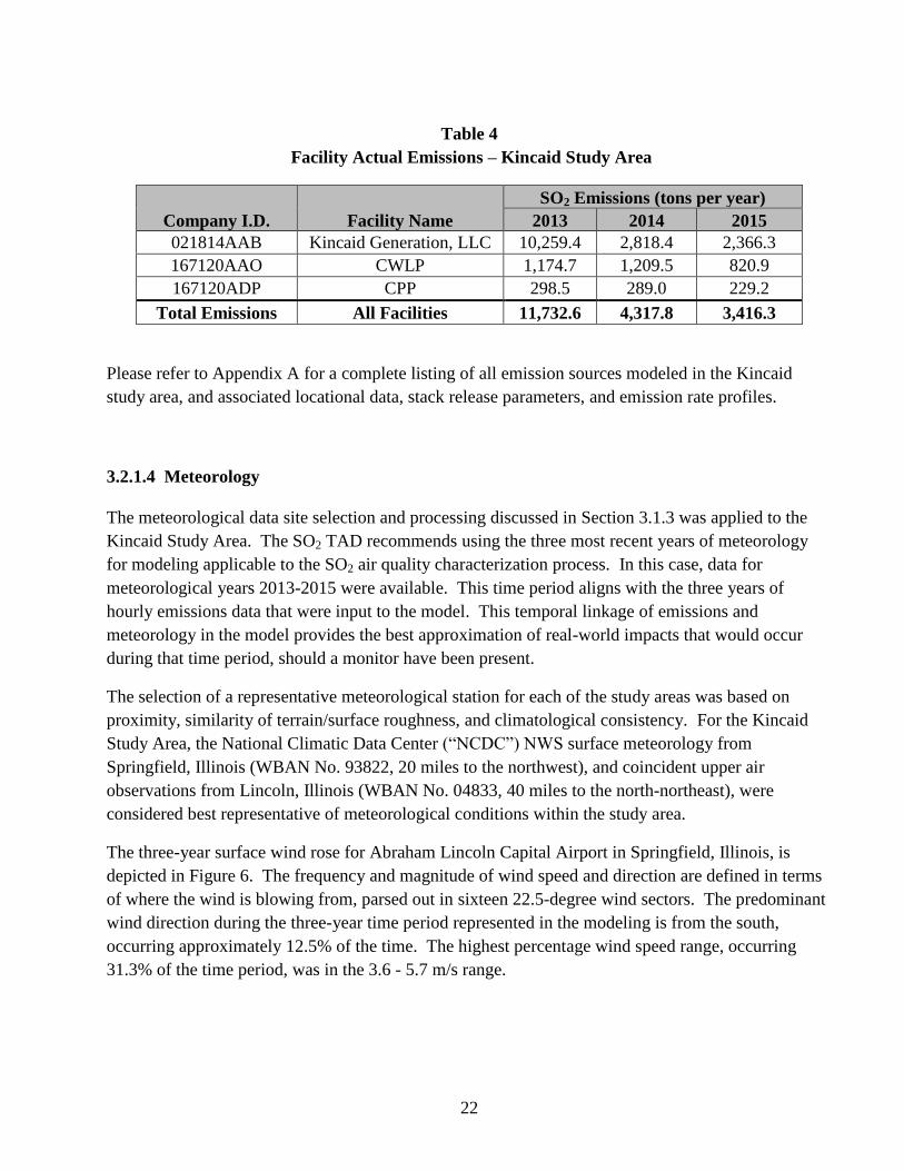
Table 4
Facility Actual Emissions – Kincaid Study Area
Company I.D. Facility Name
SO2 Emissions (tons per year)
2013 2014 2015
021814AAB Kincaid Generation, LLC 10,259.4 2,818.4 2,366.3
167120AAO CWLP 1,174.7 1,209.5 820.9
167120ADP CPP 298.5 289.0 229.2
Total Emissions All Facilities 11,732.6 4,317.8 3,416.3
Please refer to Appendix A for a complete listing of all emission sources modeled in the Kincaid
study area, and associated locational data, stack release parameters, and emission rate profiles.
3.2.1.4 Meteorology
The meteorological data site selection and processing discussed in Section 3.1.3 was applied to the
Kincaid Study Area. The SO2 TAD recommends using the three most recent years of meteorology
for modeling applicable to the SO2 air quality characterization process. In this case, data for
meteorological years 2013-2015 were available. This time period aligns with the three years of
hourly emissions data that were input to the model. This temporal linkage of emissions and
meteorology in the model provides the best approximation of real-world impacts that would occur
during that time period, should a monitor have been present.
The selection of a representative meteorological station for each of the study areas was based on
proximity, similarity of terrain/surface roughness, and climatological consistency. For the Kincaid
Study Area, the National Climatic Data Center (“NCDC”) NWS surface meteorology from
Springfield, Illinois (WBAN No. 93822, 20 miles to the northwest), and coincident upper air
observations from Lincoln, Illinois (WBAN No. 04833, 40 miles to the north-northeast), were
considered best representative of meteorological conditions within the study area.
The three-year surface wind rose for Abraham Lincoln Capital Airport in Springfield, Illinois, is
depicted in Figure 6. The frequency and magnitude of wind speed and direction are defined in terms
of where the wind is blowing from, parsed out in sixteen 22.5-degree wind sectors. The predominant
wind direction during the three-year time period represented in the modeling is from the south,
occurring approximately 12.5% of the time. The highest percentage wind speed range, occurring
31.3% of the time period, was in the 3.6 - 5.7 m/s range.

23
Figure 6
Abraham Lincoln Capital Airport
Cumulative Annual Wind Rose
2013-2015
3.2.1.5 Background SO2
The monitored background integration process discussed in Section 3.1.4.2 was applied to the
Kincaid Study Area modeling analysis. Illinois EPA incorporated temporally-varying background
one-hour concentrations developed from the Nilwood monitor, which is located approximately 22
WRPLOT View - Lakes Environmental Software
WIND ROSE PLOT:
Station #93822 - SPRINGFIELD/CAPITAL ARPT, IL
COMMENTS:
Direction Wind is blowing from.
COMPANY NAME:
MODELER:
DATE:
6/9/2016
PROJECT NO.:
NORTH
SOUTH
WEST EAST
3%
6%
9%
12%
15%
WIND SPEED
(m/s)
>= 11.1
8.8 - 11.1
5.7 - 8.8
3.6 - 5.7
2.1 - 3.6
0.5 - 2.1
Calms: 0.55%
TOTAL COUNT:
26254 hrs.
CALM WINDS:
0.55%
DATA PERIOD:
Start Date: 1/1/2013 - 00:00End Date: 12/31/2015 - 23:00
AVG. WIND SPEED:
4.28 m/s
DISPLAY:
Wind SpeedDirection (blowing from)
24
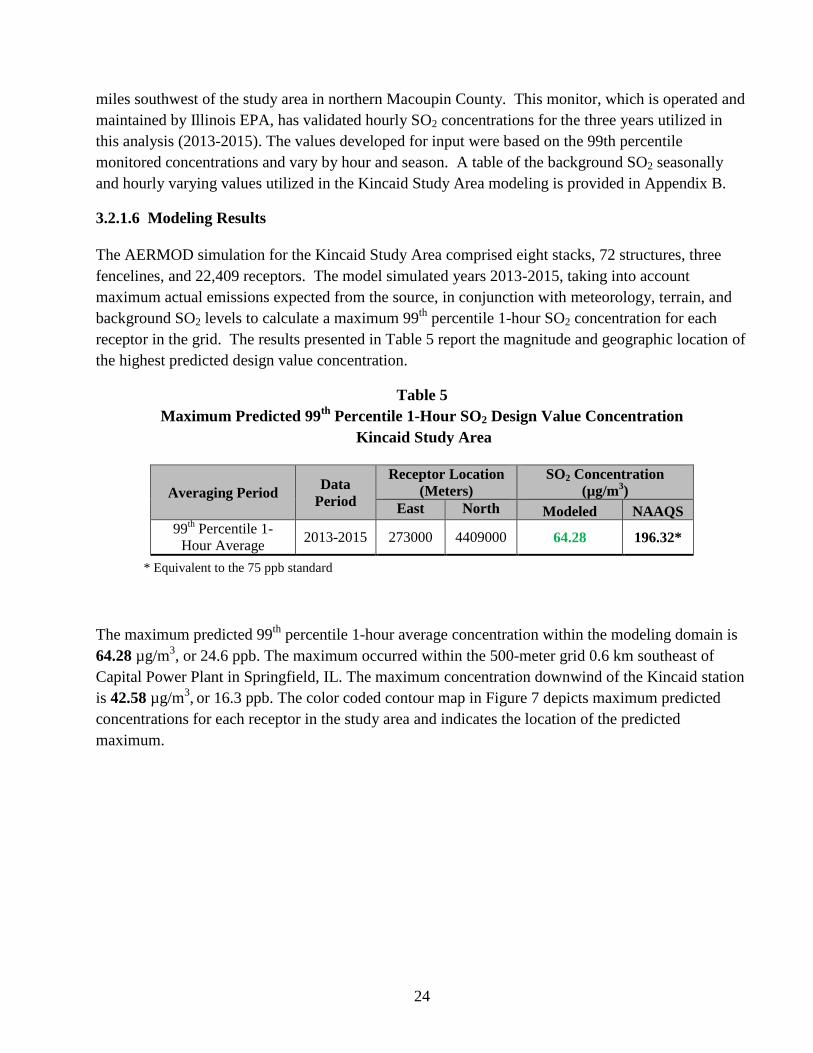
miles southwest of the study area in northern Macoupin County. This monitor, which is operated and
maintained by Illinois EPA, has validated hourly SO2 concentrations for the three years utilized in
this analysis (2013-2015). The values developed for input were based on the 99th percentile
monitored concentrations and vary by hour and season. A table of the background SO2 seasonally
and hourly varying values utilized in the Kincaid Study Area modeling is provided in Appendix B.
3.2.1.6 Modeling Results
The AERMOD simulation for the Kincaid Study Area comprised eight stacks, 72 structures, three
fencelines, and 22,409 receptors. The model simulated years 2013-2015, taking into account
maximum actual emissions expected from the source, in conjunction with meteorology, terrain, and
background SO2 levels to calculate a maximum 99th
percentile 1-hour SO2 concentration for each
receptor in the grid. The results presented in Table 5 report the magnitude and geographic location of
the highest predicted design value concentration.
Table 5
Maximum Predicted 99th
Percentile 1-Hour SO2 Design Value Concentration
Kincaid Study Area
Averaging Period Data
Period
Receptor Location
(Meters)
SO2 Concentration
(µg/m3)
East North Modeled NAAQS
99th Percentile 1-
Hour Average 2013-2015 273000 4409000 64.28 196.32*
* Equivalent to the 75 ppb standard
The maximum predicted 99th
percentile 1-hour average concentration within the modeling domain is
64.28 µg/m3, or 24.6 ppb. The maximum occurred within the 500-meter grid 0.6 km southeast of
Capital Power Plant in Springfield, IL. The maximum concentration downwind of the Kincaid station
is 42.58 µg/m3, or 16.3 ppb. The color coded contour map in Figure 7 depicts maximum predicted
concentrations for each receptor in the study area and indicates the location of the predicted
maximum.

25
Figure 7
Maximum Predicted 99th Percentile 1-Hour SO2 Concentrations – Kincaid Study Area

26
3.2.2 Rain CII Carbon LLC
Rain CII Carbon, LLC (now Rain Carbon Inc.) owns and operates a petroleum coke calcining facility
southeast of Robinson, Illinois, in eastern Crawford County, and within approximately seven to eight
miles of the Illinois-Indiana state line. As shown in Figure 8, the plant is located near the southeast
edge of town and is bounded to the north by the Marathon Petroleum Company, LLC oil refinery
(“Marathon”). The facility has two calcining lines, each processing green petroleum coke through
separate countercurrent, inclined rotary kilns (each rated at 50 mmBtu/hour) and rotary coolers. The
permitted green coke feed capacity of each kiln is 28 tons per hour. The combustion of volatile gases
from the green coke feed and the consumption (approximately 20%) of some of the green coke
provide the primary source of heat for the calcining process. The calcined coke flows by gravity from
the kiln into the cooler where it is quenched by a water spray to lower the coke temperature. Each
calcining line has an associated pyroscrubber and baghouse. Separate exhaust stacks service the kilns
and the coolers. The rotary kilns are considered to be the only significant sources of SO2 emissions at
this facility.
Figure 8
Rain CII Carbon Study Area
27
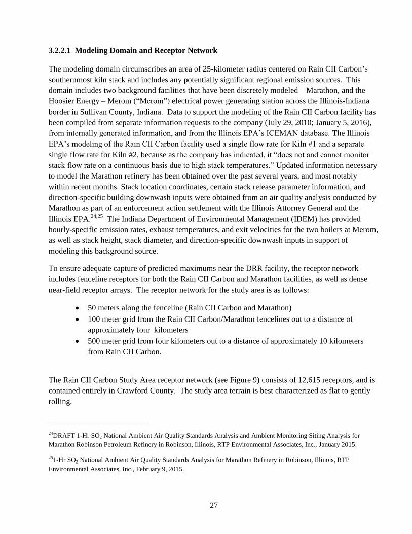
3.2.2.1 Modeling Domain and Receptor Network
The modeling domain circumscribes an area of 25-kilometer radius centered on Rain CII Carbon’s
southernmost kiln stack and includes any potentially significant regional emission sources. This
domain includes two background facilities that have been discretely modeled – Marathon, and the
Hoosier Energy – Merom (“Merom”) electrical power generating station across the Illinois-Indiana
border in Sullivan County, Indiana. Data to support the modeling of the Rain CII Carbon facility has
been compiled from separate information requests to the company (July 29, 2010; January 5, 2016),
from internally generated information, and from the Illinois EPA’s ICEMAN database. The Illinois
EPA’s modeling of the Rain CII Carbon facility used a single flow rate for Kiln #1 and a separate
single flow rate for Kiln #2, because as the company has indicated, it “does not and cannot monitor
stack flow rate on a continuous basis due to high stack temperatures.” Updated information necessary
to model the Marathon refinery has been obtained over the past several years, and most notably
within recent months. Stack location coordinates, certain stack release parameter information, and
direction-specific building downwash inputs were obtained from an air quality analysis conducted by
Marathon as part of an enforcement action settlement with the Illinois Attorney General and the
Illinois EPA.24,25
The Indiana Department of Environmental Management (IDEM) has provided
hourly-specific emission rates, exhaust temperatures, and exit velocities for the two boilers at Merom,
as well as stack height, stack diameter, and direction-specific downwash inputs in support of
modeling this background source.
To ensure adequate capture of predicted maximums near the DRR facility, the receptor network
includes fenceline receptors for both the Rain CII Carbon and Marathon facilities, as well as dense
near-field receptor arrays. The receptor network for the study area is as follows:
50 meters along the fenceline (Rain CII Carbon and Marathon)
100 meter grid from the Rain CII Carbon/Marathon fencelines out to a distance of
approximately four kilometers
500 meter grid from four kilometers out to a distance of approximately 10 kilometers
from Rain CII Carbon.
The Rain CII Carbon Study Area receptor network (see Figure 9) consists of 12,615 receptors, and is
contained entirely in Crawford County. The study area terrain is best characterized as flat to gently
rolling.
_________________________
24DRAFT 1-Hr SO2 National Ambient Air Quality Standards Analysis and Ambient Monitoring Siting Analysis for
Marathon Robinson Petroleum Refinery in Robinson, Illinois, RTP Environmental Associates, Inc., January 2015.
251-Hr SO2 National Ambient Air Quality Standards Analysis for Marathon Refinery in Robinson, Illinois, RTP
Environmental Associates, Inc., February 9, 2015.

28
Figure 9
Receptor Grid – Rain CII Carbon Study Area
3.2.2.2 Auer’s Analysis (Urban/Rural Environment)
The 25-kilometer radius study area and three kilometer near-field ring, centered on the southernmost
kiln stack at Rain CII Carbon, were evaluated for determining whether this area represents an urban
or rural dispersion regime. The results of the Auer’s analysis are presented in Figures 10 and 11 and
Table 6.

29
Figure 10
Land Cover in the Rain CII Carbon Study Area (Urban vs. Rural)
Figure 11
Land Cover within a Three-Kilometer Radius of Rain CII Carbon (Urban vs. Rural)

30
Table 6
Land Cover Percentages by Auer’s Category for a Three-Kilometer Radius Area and for
the Modeling Domain (25-Kilometer Radius) – Rain CII Carbon Study Area
The Auer’s analysis indicates that the study area is at least 99% rural and the three-kilometer near-
field is approximately 90% rural. Based upon these results, the dispersion regime was treated as
rural.
The 2011 NLCD land cover dataset erroneously classified the Rain CII Carbon facility as “Open
Water.” Due to the relatively small size of this facility, this classification error did not significantly
alter the results of the three-kilometer Auer’s Analysis. However, the problem was still addressed by
using a small 400-meter buffer to extract out all of the misclassified “Open Water” cells that fell
within the property boundary of the Rain CII Carbon facility. From this small grid extraction it was
determined that 132 cells were misclassified. The Auer’s Analysis results were then adjusted by
subtracting the 132 cells from the “Open Water” category and adding them to the “Developed, High
Intensity” category. This increased the urban land cover percentage from 8.88% to 9.30% for the
three-kilometer Auer’s Analysis and from 0.28% to 0.29% for the 25-kilometer Auer’s Analysis.
This very small adjustment did not change the final determination that the Rain CII Carbon Study
Area should be modeled as Rural.
3.2.2.3 Emissions
Illinois EPA received hourly emissions data (actual) for all sources modeled for the Rain CII Carbon
facility, as well as for the Hoosier Energy - Merom generating station and for most sources from the
Marathon Petroleum Company refinery for calendar years 2012-2015. Since the Merom generating
station is in the Eastern Time Zone, yet Rain CII Carbon and Marathon are in the Central Time Zone,
the hourly inputs for Merom were shifted back one hour in order for all three facilities to be in
synchrony. Table 7 provides a summary of the reported actual SO2 tonnages from these facilities for
2013-2015. In response to an inquiry by USEPA as to why there were significantly lower emissions
NLCD Value NLCD 2011 Description Auer's Code Auer's Class Cell Count Percentage Totals Cell Count Percentage Totals
23 Developed, Medium Intensity R2/R3 1,844 5.75% 4,788 0.22%
24 Developed, High Intensity I1/I2/C1 1,135 3.54% 1,620 0.07%
11 Open Water A5 141 0.44% 34,091 1.53%
21 Developed, Open Space A1/R4 3,552 11.09% 131,273 5.90%
22 Developed, Low Intensity R1 4,753 14.83% 22,657 1.02%
31 Barren Land (Rock/Sand/Clay) A3 0 0.00% 601 0.03%
41 Deciduous Forest A4 4,206 13.13% 388,606 17.46%
42 Evergreen Forest A4 0 0.00% 240 0.01%
43 Mixed Forest A4 0 0.00% 0 0.00%
52 Shrub/Scrub A4 0 0.00% 75 0.00%
71 Grassland/Herbaceous A3 457 1.43% 11,709 0.53%
81 Pasture/Hay A3 1,023 3.19% 93,478 4.20%
82 Cultivated Crops A2 14,818 46.24% 1,490,126 66.97%
90 Wood Wetlands A4 114 0.36% 43,642 1.96%
95 Emergent Herbaceous Wetlands A3 0 0.00% 2,286 0.10%
Total 32,043 100.00% 100.00% 2,225,192 100.00% 100.00%
Rural 90.70% 99.71%
Analysis based on 30 meter by 30 meter raster cells extracted for each area.
Rain CII Carbon Study Area Auer's Analysis Auer's 3 km Ring Study Area 25 km Ring
Urban 9.30% 0.29%

31
for Rain CII Carbon in 2015, as compared with years 2013 and 2014, the company informed the
Illinois EPA, “The SO2 emissions were lower due to low customer demands for the year, which led to
the plant operating at less than 50% capacity.” Upon receipt of the actual hourly emissions data
provided by Rain CII Carbon for the two kilns (Protocol totals were based on AER submissions for
those calendar years), emissions for 2013-2015 totaled 2,958.93; 3,134.08; and 2,161.40 tons per year
as opposed to 5,239.7; 5,429.8; and 2,161.40 tons per year per AERs and Illinois EPA’s ICEMAN
database. Illinois EPA contacted Rain CII Carbon to obtain an explanation for the discrepancy. Rain
CII stated that when the AERs were completed, they had believed that the most reliable method for
estimating SO2 emissions “used hourly emissions data from the most recent stack test and operating
hours for each kiln. This method was based on the assumption that stack test conditions represented
‘typical’ or ‘average’ operating conditions for the facility. In truth, the data from the stack tests
represent operation during high/maximum feed rates. There is ample time during 2013 and 2014 that
the kilns were not operating at high/maximum feed rates.” Upon responding to the state’s data request
in January 2016, Rain CII Carbon modified its method of estimating emissions to a more accurate
method. The company informed Illinois EPA, “The new method was based on an engineering study
that correlated SO2 emissions with actual operating data, taking into account variations in hourly feed
rate and coke sulfur levels. This is in contrast to the previous method that assumed a uniform
emission rate for all feed rates and coke sulfur levels.”
For Marathon, although the magnitude of the reported facility emissions (approximately 202 tons) for
2014 are much lower than those of Rain CII Carbon, the proximity of the refinery to the Rain CII
Carbon facility warranted its inclusion in the modeling analysis. The Hoosier Energy – Merom power
plant had reported SO2 emissions of 3,316 tons in calendar year 2014 and because of the magnitude
of the emissions and relative source proximity, its inclusion was also considered necessary.
Table 7
Facility Actual Emissions – Rain CII Carbon Study Area
Company I.D. Facility Name
SO2 Emissions (tons per year)
2013 2014 2015
033025AAJ Rain CII Carbon 2,958.9 3,134.1 2,161.4
033808AAB Marathon Petroleum 218.8 207.1 213.4
1815300005 Merom Generating
Station 2,816.2 3,315.9 2,579.4
Total Emissions All Facilities 5,993.9 6,657.1 4,954.2
The Rain CII Carbon hourly emission estimates are based upon a calculation method that takes into
account variations in hourly feed rates and coke sulfur levels. The Merom generating station hourly-
specific data was provided by IDEM and is presumed to reflect the continuous emissions monitoring
data supplied to USEPA’s Clean Air Markets Division database. The Illinois EPA had requested
hourly-specific information on this facility from USEPA, and the information received was evaluated

32
for potential use in refining the IDEM-supplied data. The Marathon Petroleum Company data for the
Fluidized Catalytic Cracking Unit, Sulfur Recovery Units, and 1F1 Crude Atmospheric Heater were
obtained from SO2 continuous emission monitoring. For Marathon’s boilers and other heaters, hourly
heat input rates in combination with fuel gas emission factors (determined from continuous emission
monitoring of H2S in refinery fuel gas) provided the basis of the hourly emissions. Non-H2S sulfur
data were incorporated into the final estimates. It should be noted that Heater 90F-41 replaced Heater
90F-1 in October 2013. SO2 emission estimates for flaring reflect the H2S content of the gases flared
and the quantity of gas being flared. Anomalous negative emission rates for Flare #4 during certain
hours in 2013 were set to zero. Day-specific operational data were provided for the stationary engines
(fire pumps) at Marathon, and together with SO2 emission rates developed from stack testing data and
horsepower ratings, a particular engine’s emissions were allocated uniformly across all hours of each
specific day of operation.
The following example calculation for the 66F-3 Sulfur Recovery Unit thermal oxidizer (January 1,
2013, hour 01) was provided by Marathon to illustrate the derivation of a lbs/hour emission rate based
upon an in-stack parts per million concentration (obtained from hourly averaged analyzer data):
In-stack ppm concentration: 8.1033 ppm
Moles SO2/hour: (311,190 SCFH SO2 x 8.1033 ppm SO2) / (106 x 379.5 SCF/lb-mol)
= 0.0066447 lb-mol SO2/hour
Where 311,190 SCFH is the calculated stack gas rate on a dry basis, and 106 is used to determine the
decimal fraction of 8.1033 ppmv, i.e. 8.1033 ppm/1,000,000 = 8.1033 x 10⁻⁶
Lbs SO2/hour: (0.0066447 lb-mol SO2/hour) x (64.06 lb/lb-mole SO2) = 0.4257 lb/hr SO2
Where 64.06 lb/lb-mole SO2 is the molar mass of SO2.
Please refer to Appendix A for a complete listing of all emission sources modeled in the Rain CII
Carbon study area, and their associated locational data, stack release parameters, and emission rates.
3.2.2.4 Meteorology
As discussed in Section 3.1.3, the meteorological data site selection and processing procedure was
applied to the Rain CII Carbon Study Area. NCDC NWS surface meteorology from Evansville,
Indiana (WBAN No. 93817, 65 miles to the south-southeast), and coincident upper air observations
from Lincoln, Illinois (WBAN No. 04833, 115 miles to the north-northwest), were determined to be
best representative of meteorological conditions within the study area.
The three-year surface wind rose for Evansville Regional Airport in Evansville, Indiana, is depicted
in Figure 12. The frequency and magnitude of wind speed and direction are defined in terms of
where the wind is blowing from, parsed out in sixteen 22.5-degree wind sectors. The predominant
wind direction during the three-year time period proposed in the modeling is from the south-

33
southwest, occurring approximately 10.6% of the time. The highest percentage wind speed range,
occurring 31.3% of the time, was in the 2.1 - 3.6 m/s range.
Figure 12
Evansville Regional Airport, Indiana
Cumulative Annual Wind Rose
2013-2015
WRPLOT View - Lakes Environmental Software
WIND ROSE PLOT:
Station #93817 - EVANSVILLE/DRESS REGIONAL ARP, IN
COMMENTS:
Direction Wind is blowing from.
COMPANY NAME:
MODELER:
DATE:
6/9/2016
PROJECT NO.:
NORTH
SOUTH
WEST EAST
3%
6%
9%
12%
15%
WIND SPEED
(m/s)
>= 11.1
8.8 - 11.1
5.7 - 8.8
3.6 - 5.7
2.1 - 3.6
0.5 - 2.1
Calms: 1.15%
TOTAL COUNT:
26206 hrs.
CALM WINDS:
1.15%
DATA PERIOD:
Start Date: 1/1/2013 - 00:00End Date: 12/31/2015 - 23:00
AVG. WIND SPEED:
3.28 m/s
DISPLAY:
Wind SpeedDirection (blowing from)

34
3.2.2.5 Background SO2
The process of incorporating monitored background data as discussed in Section 3.1.4.2 was applied
in the Rain CII Carbon Study Area modeling analysis. Illinois EPA incorporated temporally-varying
background one-hour concentrations developed from the Nilwood monitor, which is located
approximately 115 miles west-northwest of the study area in northern Macoupin County. The
monitor, which is operated and maintained by Illinois EPA, has validated hourly SO2 concentrations
for the three years proposed to be utilized in this analysis (2013-2015). The values developed for
input are based on the 99th
percentile monitored concentrations and vary by hour and season. A table
of the proposed background SO2 seasonally and hourly varying values used in the Rain CII Carbon
Study Area modeling is provided in Appendix B.
3.2.2.6 Modeling Results
The AERMOD simulation for the Rain CII Study Area comprised 58 stacks, 262 structures, two
fencelines, and 12,615 receptors. The model simulated year 2013-2015, while taking into account
maximum actual emissions expected from the source, in conjunction with meteorology, terrain, and
background SO2 levels to calculate a maximum 99th
percentile 1-hour SO2 concentration for each
receptor in the grid. The results presented in Table 8 report the magnitude and geographic location of
the highest predicted design value concentration.
Table 8
Maximum Predicted 99th
Percentile 1-Hour SO2 Design Value Concentration
Rain CII Study Area
Averaging Period Data
Period
Receptor Location
(Meters)
SO2 Concentration
(µg/m3)
East North Modeled NAAQS
99th Percentile 1-
Hour Average 2013-2015 437364 4316246 105.01 196.32*
* Equivalent to the 75 ppb standard
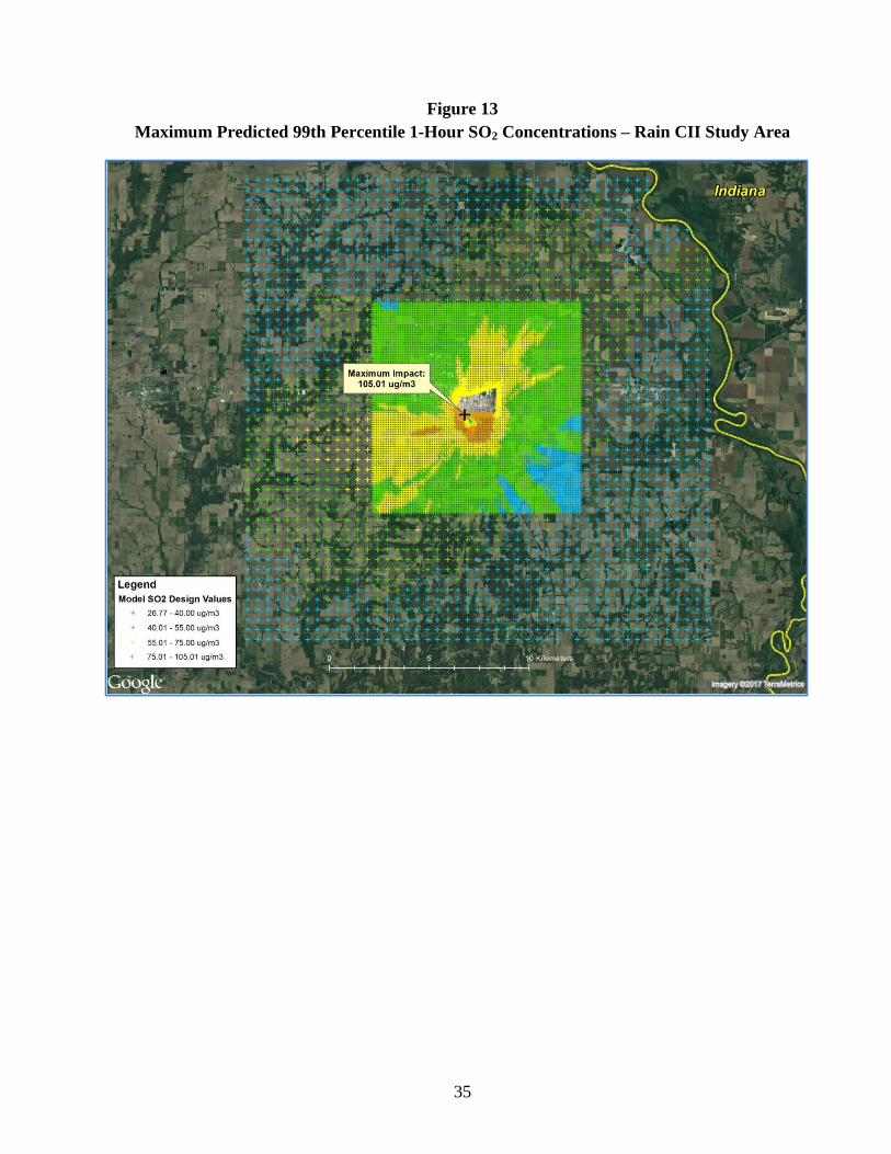
The maximum predicted 99th
percentile 1-hour average concentration within the modeling domain is
105.01 µg/m3, or 40.1 ppb. The maximum occurred within the 100-meter grid 0.4 km northwest of
Rain CII’s northern pyro-scrubber stack. The color coded contour map in Figure 13 depicts
maximum predicted concentrations for each receptor in the study area and indicates the location of
the predicted maximum.
35
Figure 13
Maximum Predicted 99th Percentile 1-Hour SO2 Concentrations – Rain CII Study Area

36
3.2.3 Midwest Generation LLC – Waukegan
NRG Energy Inc. (“NRG”) owns the Midwest Generation LLC – Waukegan (Waukegan Station)
electrical power generating station located in Lake County, along a section of western Lake Michigan
coastal area in the City of Waukegan (see Figure 14). The company operates two coal-fired boilers
(Unit #7 and Unit #8) with nominal capacities of 3,255 and 3,262 mmBtu/hour, and these boilers also
have the capability of firing natural gas and/or fuel oil either with or without coal. SO2 emissions are
controlled through dry sorbent injection of trona and the associated use of electrostatic precipitators.
The company operates four distillate oil-fired turbines, each with a nominal capacity of 552.6
mmBtu/hour, to meet peak power demands. A natural gas-fired auxiliary boiler, with a nominal
capacity of 51.1 mmBtu/hour, is used to provide steam for building heat and other internal purposes,
but not for electricity generation by the steam turbine generators.
Figure 14
Midwest Generation LLC - Waukegan Study Area
3.2.3.1 Modeling Domain and Receptor Network
The modeling domain for the Waukegan Station and all potentially significant regional emission
sources is centered on the generating station’s southernmost primary boiler stack and extends outward
to encompass an area of 30-kilometer radius. In addition to the Waukegan Station, this domain

37
includes eight background sources (Abbvie Inc.; New NGC Inc.; Advanced Disposal Services Zion
Landfill Inc.; Bio Energy (Illinois) LLC; Abbott Laboratories; Countryside Genco, LLC; Countryside
Landfill; and Wisconsin’s Pleasant Prairie Generating Station). To ensure adequate capture of
predicted maximums near the DRR facility, the receptor network includes fenceline receptors and a
dense near-field receptor array. The receptor network for the study area includes the following:
50 meters along fencelines (Waukegan Station, New NGC, Abbvie, Abbott Laboratories,
Advanced Disposal Services Zion Landfill, and Bio Energy (Illinois))
100 meters from the Waukegan Station out to a distance of approximately four kilometers
500 meters from four kilometers out to a distance of approximately 10 kilometers from
the Waukegan Station.
The Waukegan Study Area receptor network (see Figure 15) consists of 6,098 receptors, and is
contained entirely in Lake County. Per the recommendation of the TAD, receptors were not placed
on large water bodies (Lake Michigan). The study area terrain is best characterized as flat to gently
rolling.
Figure 15
Receptor Grid – Waukegan Study Area

38
3.2.3.2 Auer’s Analysis (Urban/Rural Environment)
The 30-kilometer study area and three-kilometer near-field ring applied in the Auer’s analysis for the
Waukegan Study Area are both centered on the southernmost primary boiler stack at Waukegan
Station. The results of the Auer’s analysis for the Waukegan Study Area are presented in Figure 16,
Figure 17, and Table 9.
Figure 16
Land Cover in the Waukegan Study Area
(Urban vs. Rural)

39
Figure 17
Land Cover within a Three-Kilometer Radius of Waukegan Station (Urban vs. Rural)
Table 9
Land Cover Percentages by Auer’s Category for a Three-Kilometer Radius Area and for
the Modeling Domain (30-Kilometer Radius) – Waukegan Study Area
NLCD Value NLCD 2011 Description Auer's Code Auer's Class Cell Count Percentage Totals Cell Count Percentage Totals
23 Developed, Medium Intensity R2/R3 3,755 11.79% 175,101 5.50%
24 Developed, High Intensity I1/I2/C1 2,421 7.60% 67,206 2.11%
11 Open Water A5 13,342 41.89% 1,612,299 50.64%
21 Developed, Open Space A1/R4 2,246 7.05% 256,320 8.05%
22 Developed, Low Intensity R1 3,692 11.59% 391,686 12.30%
31 Barren Land (Rock/Sand/Clay) A3 893 2.80% 6,584 0.21%
41 Deciduous Forest A4 1,069 3.36% 161,115 5.06%
42 Evergreen Forest A4 44 0.14% 859 0.03%
43 Mixed Forest A4 91 0.29% 19,318 0.61%
52 Shrub/Scrub A4 7 0.02% 5,202 0.16%
71 Grassland/Herbaceous A3 202 0.63% 49,433 1.55%
81 Pasture/Hay A3 0 0.00% 62,997 1.98%
82 Cultivated Crops A2 0 0.00% 265,513 8.34%
90 Wood Wetlands A4 620 1.95% 72,447 2.28%
95 Emergent Herbaceous Wetlands A3 3,467 10.89% 37,720 1.18%
Total 31,849 100.00% 100.00% 3,183,800 100.00% 100.00%
Study Area 30 km Ring
7.61%
92.39%
Analysis based on 30 meter by 30 meter raster cells extracted for each area.
Rural
19.39%
80.61%
Auer's 3 km Ring
Urban
Waukegan Study Area Auer's Analysis

40
The Auer’s analysis indicates that the study area is at least 92% rural and the three-kilometer near-
field is approximately 81% rural. Based upon these results, the dispersion regime will be treated as
rural.
3.2.3.3 Emissions
Illinois EPA has acquired or developed high quality emissions data for the nine facilities in the
Waukegan Study Area for the most recent years of operation. Agency staff produced refined hourly
emission temporalizations for those sources in which hourly-specific data from continuous emission
monitoring was not available. For the Waukegan Station, the parent company NRG provided hourly-
specific SO2 emission rates for Unit #7 and Unit #8 for calendar years 2012-2015. NRG also
provided annual SO2 emission totals and total hours of operation for each of the turbine peaker units
during the years 2012-2015. This latter information was temporally adjusted by Illinois EPA staff to
hourly rates consistent with procedures identified in the modeling guidance TAD. Hourly-specific
SO2 emission rates and estimated hourly stack gas exit temperatures and velocities were modeled for
the WE Energies – Pleasant Prairie power plant (Pleasant Prairie, Wisconsin) based upon information
provided by USEPA. Other modeling inputs for the Pleasant Prairie power plant were previously
obtained from staff at the Wisconsin DNR. The development of emission rates for all other sources
modeled in the Waukegan study area has adhered to the recommendations in the modeling TAD.
Reported actual annual SO2 tonnages for 2013-2015 are presented in Table 10 for the DRR facility
and the background source facilities that were modeled. The magnitude of the emissions of these
background sources may individually be several orders (or more) less than those of the Waukegan
Station. Despite this, the potential for cumulative impacts that may exceed the one-hour SO2
NAAQS warranted their inclusion.
Table 10
Facility Actual Emissions – Waukegan Study Area
Company I.D. Facility Name
SO2 Emissions (tons per year)
2013 2014 2015
097190AAC Midwest Generation LLC –
Waukegan 7,749.9 5792.4 2,339.3
097190AAP New NGC Inc. 8.7 8.7 8.7
097025AAR Countryside Genco LLC 27.1 53.1 41.5
097806AAG Countryside Landfill 23.9 6.3 14.5
097809AAD Abbott Laboratories 74.0 22.8 0.2
097125AAA AbbVie Inc. 59.5 16.2 6.6
097200AAV ADS Zion Landfill Inc. 48.1 28.4 26.7
097200ABC Bio Energy (Illinois) LLC 40.9 24.7 22.3
230006260 Pleasant Prairie Generating Station 1,173.8 1,310.1 1,335.5
Total
Emissions All Facilities 9205.9 7262.7 3795.3

41
The emissions reported in Table 10 in 2014 for Waukegan Station differ from the modeling protocol
totals (5792.4 vs. 7683.4). The company provided revised data due to an inadvertent reporting of the
hours of operation in the total tons column of the company-submitted AER for Boiler Unit 8. The
corrected emissions tonnages for the plant are provided below and also reflected in the model.
Please refer to Appendix A for a complete listing of all emission sources modeled in the Waukegan
study area, and the associated locational data, stack release parameter data, and emission rate profiles.
3.2.3.4 Meteorology
The same meteorological data site selection and processing procedure used in the previous study
areas was applied to the Waukegan Study Area. As described in the protocol, Illinois proposed the
use of surface NWS meteorology from Milwaukee Wisconsin (40 miles north of the Waukegan
station), but promised investigation into the viability of utilizing the data from nearby Waukegan
National Airport (3.5 miles northwest of Waukegan station). Milwaukee’s General Mitchell Airport is
a first order NWS station, while Waukegan National Airport is a Second Order station. After analysis
of the Waukegan data and comparison of completeness (i.e., calms, missing) relative to the
Milwaukee site, Illinois EPA found a negligible difference (less than 0.07 percent) in the number of
calms and missing hours between the two sites. In addition, the Waukegan site had greater data
completeness for cloud cover and temperature data than the Milwaukee site. Consequently, Illinois
EPA considered the Waukegan National Airport data more robust and more representative
geographically and opted to perform the modeling for the study area using that meteorology.
NCDC NWS surface meteorology from Waukegan, Illinois (WBAN No. 14880, 3.5 miles to the
northwest), and coincident upper air observations from Davenport, Iowa (WBAN No. 14923, 152
miles to the southwest), were considered reasonably representative of meteorological conditions
within the study area.
The three-year surface wind rose for Waukegan National Airport is depicted in Figure 18. The
frequency and magnitude of wind speed and direction are defined in terms of where the wind is
blowing from, parsed out in sixteen 22.5-degree wind sectors. The predominant wind direction
during the three-year time period proposed in the modeling is from the southwest, occurring
approximately 12.7% of the time. The highest percentage wind speed range, occurring 33.0% of the
time period, was in the 3.6 - 5.7 m/s range.

42
Figure 18
Waukegan National Airport, Waukegan, Illinois
Cumulative Annual Wind Rose
2013-2015
WRPLOT View - Lakes Environmental Software
WIND ROSE PLOT:
Station #14880
COMMENTS:
Direction Wind is blowing from.
COMPANY NAME:
MODELER:
DATE:
12/8/2016
PROJECT NO.:
NORTH
SOUTH
WEST EAST
3%
6%
9%
12%
15%
WIND SPEED
(m/s)
>= 11.1
8.8 - 11.1
5.7 - 8.8
3.6 - 5.7
2.1 - 3.6
0.5 - 2.1
Calms: 0.54%
TOTAL COUNT:
26213 hrs.
CALM WINDS:
0.54%
DATA PERIOD:
Start Date: 1/1/2013 - 00:00End Date: 12/31/2015 - 23:00
AVG. WIND SPEED:
3.73 m/s
DISPLAY:
Wind SpeedDirection (blowing from)

43
3.2.3.5 Background SO2
The Northbrook and Oglesby, Illinois, monitors were evaluated for use as background SO2 monitors
for the Waukegan Study Area. Although the Northbrook monitor is much closer to the study area, the
data completeness percentage was too low to consider it a viable background site for the modeling.
The Oglesby monitor is located approximately 98 miles southwest of the center of the study area in
LaSalle County. This monitor, which is operated and maintained by Illinois EPA, has validated
hourly SO2 concentrations for the three years proposed to be utilized in this analysis (2013-2015).
Illinois EPA incorporated temporally-varying background one-hour concentrations developed from
the Oglesby monitor. The values developed for input were based on the 99th percentile monitored
concentrations and vary by hour and season in the same manner as discussed previously in Section
3.1.4.2. A table of the background SO2 seasonally and hourly varying values is provided in Appendix
B.
3.2.3.6 Modeling Results
The AERMOD simulation for the Waukegan Study Area comprised 34 stacks, 70 structures, seven
fencelines, and 6,031 receptors. The model simulated year 2013-2015, taking into account maximum
actual emissions expected from the source, in conjunction with meteorology, terrain, and background
SO2 levels to calculate a maximum 99th
percentile 1-hour SO2 concentration for each receptor in the
grid. The results presented in Table 11 report the magnitude and geographic location of the highest
predicted design value concentration.
Table 11
Maximum Predicted 99th
Percentile 1-Hour SO2 Design Value Concentration
Waukegan Study Area
Averaging Period Data
Period
Receptor Location
(Meters)
SO2 Concentration
(µg/m3)
East North Modeled NAAQS
99th Percentile 1-
Hour Average 2013-2015 427419 4703366 98.91 196.32*
* Equivalent to the 75 ppb standard
The maximum predicted 99th
percentile 1-hour average concentration within the modeling domain is
98.91 µg/m3, or 37.8 ppb. The maximum occurred along the Advanced Disposal Services fenceline
(50 meter spacing), approximately 12.3 km northwest of the Waukegan Station in Zion, IL. The
maximum concentration downwind of the Waukegan Station is 53.61 µg/m3, or 20.5 ppb. The color
coded contour map in Figure 19 depicts maximum predicted concentrations for each receptor in the
study area and indicates the location of the predicted maximum.

44
Figure 19
Maximum Predicted 99th Percentile 1-Hour SO2 Concentrations – Waukegan Study Area

45
3.2.4 Dynegy Midwest Generation – Baldwin/Prairie State Generating Station
The Dynegy Midwest Generation Inc. – Baldwin Power Plant (“DMG – Baldwin”) is located just
outside the community of Baldwin, in Randolph County. The Illinois EPA air emissions inventory
system indicates that DMG – Baldwin has four SO2-emitting sources: three steam electric coal-fired
generating units that are nominally rated at 584 megawatts (Boiler #1), 586 megawatts (Boiler #2),
and 627 megawatts (Boiler #3), and an oil-fired auxiliary heating boiler that is nominally rated at 130
mmBtu/hour. SO2 emissions from the three steam electric coal-fired generating units are controlled
by flue gas desulfurization systems (sorbent injection and scrubbers) and exhaust through separate
unobstructed vertical stacks. The uncontrolled auxiliary heating boiler has horizontally-directed
exhaust, and the exhaust exit velocity was adjusted (in accordance with federal modeling guidance) to
minimize mechanically-induced plume rise.
Approximately 25 kilometers to the east of DMG – Baldwin, near the town of Lively Grove in rural
Washington County, is the Prairie State Generating Company (“PSGC”) power plant. The company
operates two pulverized coal boilers – each with a maximum rated capacity of approximately 7,500
mmBtu/hour – an auxiliary natural gas-fired boiler, and two emergency engines burning ultra-low
sulfur diesel fuel. SO2 emissions from the power generation boilers are controlled through wet flue
gas desulfurization (scrubbers) in separate air pollution control trains, and released to the atmosphere
through separate flues in a common stack.
3.2.4.1 Modeling Domain and Receptor Network
The modeling domain for capturing regional emission sources is centered on the PSGC main stack
and extends outward to encompass an area with 50-kilometer radius. As depicted in Figure 20, this
domain includes the Baldwin and Prairie State plants and two background sources (U. S. Minerals
Inc. and Cottonwood Hills Recycling & Disposal).

46
Figure 20
Baldwin and Prairie State Generating Station Study Area
To ensure adequate capture of predicted maximums near the DMG – Baldwin and PSGC facilities,
the receptor network includes fenceline receptors and a dense near-field receptor array. The receptor
network for the study area is as follows:
50 meters along the fencelines (DMG – Baldwin, PSGC, U.S. Minerals, and Cottonwood
Hills)
100 meters from the DMG – Baldwin and PSGC fencelines out to a distance of
approximately four kilometers
500 meters from four kilometers out to a distance of approximately 20 kilometers from
both main power plants.
The DMG – Baldwin and PSGC receptor network (see Figure 21) consists of 20,485 receptors, and is
centered approximately at a midpoint between the two large power plants. The grid encompasses

47
portions of Randolph, Washington, St. Clair, and Perry Counties in Illinois. Per the recommendation
of the TAD, receptors were not placed on large water bodies (Mississippi River and Lake Baldwin).
The study area terrain is best characterized as flat to gently rolling.
Figure 21
Receptor Grid
Baldwin and Prairie State Generating Station Study Area
3.2.4.2 Auer’s Analysis (Urban/Rural Environment)
An Auer’s analysis was applied to the Baldwin and Prairie State Generating Station Study Area.
Figures 22 and 23 graphically depict the near-field areas (three-kilometer rings) applied in the Auer’s
analysis to the DMG – Baldwin and PSGC plants, respectively. Table 9 provides a statistical
breakdown by land cover category for both three-kilometer rings. The same analysis encompassing
the full study area is provided in Figure 24 and Tables 12 and 13.

48
Figure 22
Land Cover within a Three-Kilometer Radius of the Baldwin Plant
(Urban vs. Rural)
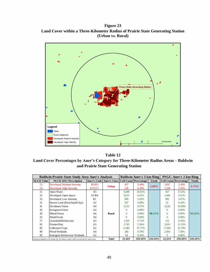
49
Figure 23
Land Cover within a Three-Kilometer Radius of Prairie State Generating Station
(Urban vs. Rural)
Table 12
Land Cover Percentages by Auer’s Category for Three-Kilometer Radius Areas – Baldwin
and Prairie State Generating Station
NLCD Value NLCD 2011 Description Auer's Code Auer's Class Cell Count Percentage Totals Cell Count Percentage Totals
23 Developed, Medium Intensity R2/R3 457 1.46% 1,057 3.30%
24 Developed, High Intensity I1/I2/C1 136 0.43% 1,104 3.45%
11 Open Water A5 9,298 29.61% 167 0.52%
21 Developed, Open Space A1/R4 2,013 6.41% 1,444 4.51%
22 Developed, Low Intensity R1 949 3.02% 982 3.07%
31 Barren Land (Rock/Sand/Clay) A3 307 0.98% 61 0.19%
41 Deciduous Forest A4 3,131 9.97% 3,228 10.08%
42 Evergreen Forest A4 0 0.00% 0 0.00%
43 Mixed Forest A4 0 0.00% 0 0.00%
52 Shrub/Scrub A4 0 0.00% 0 0.00%
71 Grassland/Herbaceous A3 1,164 3.71% 112 0.35%
81 Pasture/Hay A3 1,745 5.56% 3,635 11.35%
82 Cultivated Crops A2 11,861 37.77% 17,865 55.79%
90 Wood Wetlands A4 246 0.78% 2,364 7.38%
95 Emergent Herbaceous Wetlands A3 94 0.30% 0 0.00%
Total 31,401 100.00% 100.00% 32,019 100.00% 100.00%Analysis based on 30 meter by 30 meter raster cells extracted for each area.
Rural
1.89%
98.11%
Baldwin Auer's 3 km Ring
Urban
Baldwin-Prairie State Study Area Auer's Analysis PSGC Auer's 3 km Ring
6.75%
93.25%

50
Figure 24
Land Cover in the Baldwin and Prairie State Generating Station Study Area
(Urban vs. Rural)
Table 13
Land Cover Percentages by Auer’s Category for the Modeling Domain (50-Kilometer
Radius) – Baldwin and Prairie State Generating Station Study Area
NLCD Value NLCD 2011 Description Auer's Code Auer's Class Cell Count Percentage Totals
23 Developed, Medium Intensity R2/R3 92,258 1.04%
24 Developed, High Intensity I1/I2/C1 19,620 0.22%
11 Open Water A5 202,691 2.28%
21 Developed, Open Space A1/R4 431,525 4.85%
22 Developed, Low Intensity R1 365,733 4.11%
31 Barren Land (Rock/Sand/Clay) A3 14,458 0.16%
41 Deciduous Forest A4 1,695,685 19.07%
42 Evergreen Forest A4 1,446 0.02%
43 Mixed Forest A4 1,886 0.02%
52 Shrub/Scrub A4 341 0.00%
71 Grassland/Herbaceous A3 151,951 1.71%
81 Pasture/Hay A3 1,819,610 20.46%
82 Cultivated Crops A2 3,830,733 43.08%
90 Wood Wetlands A4 248,303 2.79%
95 Emergent Herbaceous Wetlands A3 15,959 0.18%
Total 8,892,199 100.00% 100.00%
98.74%
Baldwin-Prairie State Study Area Auer's Analysis Study Area 50 km Ring
1.26%Urban
Rural
Analysis based on 30 meter by 30 meter raster cells extracted for each area.
51
The Auer’s analysis indicates the study area is at least 98% rural and the three-kilometer near-field
areas for both power stations are over 93% rural. Based upon these results, the dispersion regime was
treated as rural.
3.2.4.3 Emissions
Illinois EPA received or developed emissions inputs for the four facilities in the Baldwin and Prairie
State Generating Station Study Area for the most recent years of operation. Hourly SO2 emission
rates based upon continuous emission monitoring were available for the large electrical power
generation boilers. For other sources, such as backup generators and fire pumps, Illinois EPA
examined fuel usage data and other available information to determine hourly emissions.
Hourly-specific SO2 emission rates for the DMG – Baldwin coal-fired generating units (Boiler #1,
Boiler #2, and Boiler #3) were provided by Dynegy Inc. for calendar years 2012-2015. For the
auxiliary heating boiler, monthly fuel usage (gallons of #2 fuel oil) and operating time (hours per
calendar month) were provided for the same period. Based on the calculated SO2 emissions from the
auxiliary boiler (0.004 tons in highest year) and operating hours of less than 50 hours in any year, the
Illinois EPA deemed emissions too low and intermittent to be applicable to the form of the 1-hour
SO2 standard for this analysis. Consequently, it was not included in the model. This determination
also applies for the diesel engines and fire pumps at the facility.
Prairie State Generating Company provided hourly-specific temperature, flow rate, and emissions
data for both of the pulverized coal-fired boilers (Unit #1 and Unit #2), and hourly emissions data
computed from gas consumption records and AP-42 emission factors for the auxiliary boiler. The
data for all boilers were for the period 2012-2015. Hourly data for Unit #1 contains an outage due to a
boiler tube leak during the very latter part of December 2015. The company also provided annual
hours of operation for both the emergency diesel fire pump and the emergency diesel generator
during this four-year period. Emission estimates for these two sources were calculated based upon
emission factors from the company’s AER, and the emissions and operating time were determined to
be too low and, consequently, were not included in the modeling.
Total actual emissions reported for both the DMG – Baldwin facility and the PSGC facility for years
2013-2015 are provided in Table 14, together with the annual emission totals for the two background
sources (U.S. Minerals Inc. and Cottonwood Hills Recycling & Disposal). The quantity of emissions
for these background sources are orders of magnitude less than those of the power plants, but given
their proximity to the power plants, they were included in the modeling simulations to assure
adequate consideration and assessment of areas of potential high local impact.

52
Table 14
Facility Actual Emissions – Baldwin and Prairie State Generating Station Study Area
Company I.D. Facility Name
SO2 Emissions (tons per year)
2013 2014 2015
157851AAA DMG Baldwin 4,803.4 4,409.5 4,160.0
189808AAB Prairie State Generating Station 4,719.5 5,696.0 7,847.6
157851AAC U. S. Minerals Inc. 3.1 3.5 1.0
163075AAL Cottonwood Hills Recycling &
Disposal 17.0 21.8 24.3
Total
Emissions All Facilities 9,543.0 10,130.8 12,032.9
Please refer to Appendix A for a complete listing of all emission sources modeled in the Baldwin and
Prairie State Generating Station study area, and the associated locational data, stack release
parameters, and emission rate profiles.
3.2.4.4 Meteorology
The same meteorological data site selection and processing procedure used for the previous study
area was applied to the Baldwin and Prairie State Generating Station Study Area. NCDC NWS
surface meteorology from St. Louis, Missouri (WBAN No. 13994, 50 miles to the northwest), and
coincident upper air observations from Lincoln, Illinois (WBAN No. 04833, 130 miles to the north-
northeast), were considered reasonably representative of meteorological conditions within this study
area.
The three-year surface wind rose for Lambert – St. Louis International Airport (St. Louis, MO) is
depicted in Figure 25. The frequency and magnitude of wind speed and direction are defined in terms
of where the wind is blowing from, parsed out in sixteen 22.5-degree wind sectors. The predominant
wind direction during the three-year time period evaluated in the modeling is from the south,
occurring approximately 9.6% of the time. The highest percentage wind speed range, occurring
34.6% of the time period, was in the 3.6 - 5.7 m/s range.
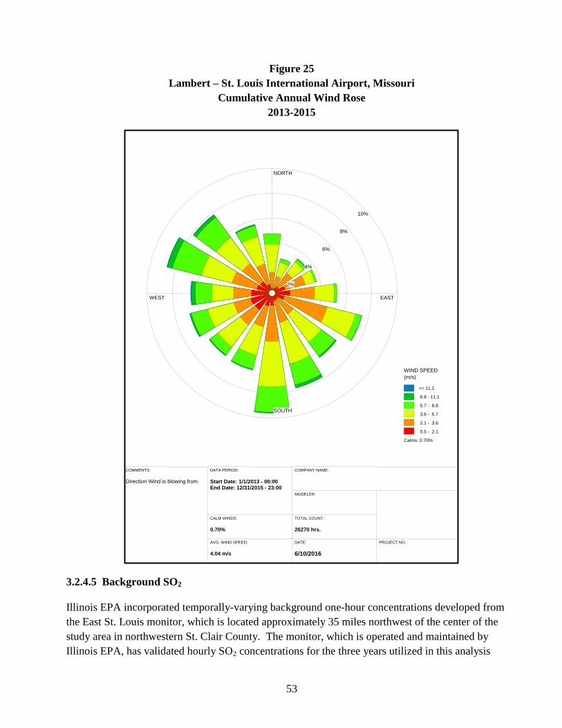
53
Figure 25
Lambert – St. Louis International Airport, Missouri
Cumulative Annual Wind Rose
2013-2015
3.2.4.5 Background SO2
Illinois EPA incorporated temporally-varying background one-hour concentrations developed from
the East St. Louis monitor, which is located approximately 35 miles northwest of the center of the
study area in northwestern St. Clair County. The monitor, which is operated and maintained by
Illinois EPA, has validated hourly SO2 concentrations for the three years utilized in this analysis
WRPLOT View - Lakes Environmental Software
WIND ROSE PLOT:
Station #13994 - ST LOUIS/LAMBERT INT'L ARPT, MO
COMMENTS:
Direction Wind is blowing from.
COMPANY NAME:
MODELER:
DATE:
6/10/2016
PROJECT NO.:
NORTH
SOUTH
WEST EAST
2%
4%
6%
8%
10%
WIND SPEED
(m/s)
>= 11.1
8.8 - 11.1
5.7 - 8.8
3.6 - 5.7
2.1 - 3.6
0.5 - 2.1
Calms: 0.70%
TOTAL COUNT:
26270 hrs.
CALM WINDS:
0.70%
DATA PERIOD:
Start Date: 1/1/2013 - 00:00End Date: 12/31/2015 - 23:00
AVG. WIND SPEED:
4.04 m/s
DISPLAY:
Wind SpeedDirection (blowing from)

54
(2013-2015). The values developed for input were based on the 99th percentile monitored
concentrations and vary by hour and season. A table of the proposed background SO2 seasonally and
hourly varying values used in the Baldwin and Prairie State Generating Station Study Area modeling
is provided in Appendix B.
3.2.4.6 Modeling Results
The AERMOD simulation for the Baldwin and Prairie State Generating Station Study Area
comprised nine stacks, 143 structures, four fencelines, and 20,485 receptors. The model simulated
years 2013-2015, taking into account maximum actual emissions expected from the source, in
conjunction with meteorology, terrain, and background SO2 levels to calculate a maximum 99th
percentile 1-hour SO2 concentration for each receptor in the grid. The results presented in Table 15
report the magnitude and geographic location of the highest predicted design value concentration.
Table 15
Maximum Predicted 99th
Percentile 1-Hour SO2 Design Value Concentration
Baldwin and Prairie State Generating Study Area
Averaging Period Data
Period
Receptor Location
(Meters)
SO2 Concentration
(µg/m3)
East North Modeled NAAQS
99th Percentile 1-
Hour Average 2013-2015 269200 4241200 78.21 196.32*
* Equivalent to the 75 ppb standard
The maximum predicted 99th
percentile 1-hour average concentration within the modeling domain is
78.21 µg/m3, or 29.9 ppb, and occurred approximately 2.8 km northeast of the Prairie State
Generating Station. The maximum concentration predicted downwind of the Baldwin Plant is 72.80
µg/m3, or 27.8 ppb. The color coded contour map in Figure 26 depicts maximum predicted
concentrations for each receptor in the study area and indicates the location of the predicted
maximum.
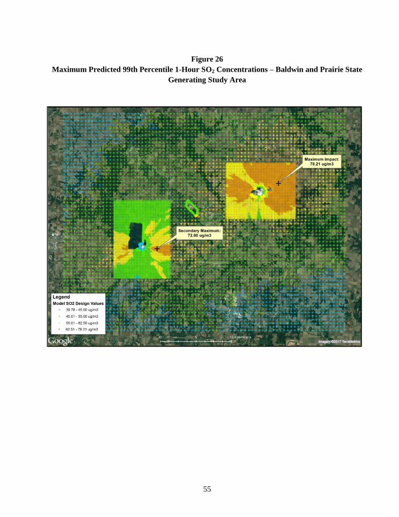
55
Figure 26
Maximum Predicted 99th Percentile 1-Hour SO2 Concentrations – Baldwin and Prairie State
Generating Study Area

56
4.0 Air Quality Characterization: Ambient Monitoring
Archer Daniels Midland Company (Decatur, IL) and Tate & Lyle Ingredients Americas (Decatur, IL)
had SO2 emissions of 9,961 and 4,379 tons, respectively, in calendar year 2014. These companies
have jointly requested that the air quality characterization for their facilities and surrounding area be
accomplished through ambient air monitoring. The monitoring commenced by January 1, 2017, and
will continue beyond January 1, 2020. This collaborative arrangement has included the development
and design of a monitoring plan,25,26,27,28
which has been approved by the Illinois EPA and USEPA
Region 5. Preceding this approval, Illinois EPA responded to comments received from USEPA on the
revised monitoring plan (dated July 22, 2016) in a conference call on September 13, 2016, and
forwarded supplementary information requested by USEPA during the call. The monitoring network
will consist of instrumentation at three locations – one site just north of the ADM - Decatur East
complex (Figure 27), and the remaining two sites in proximity (a northwesterly site and a
southeasterly site) to Tate & Lyle (Figures 28 and 29). The expansion of the Illinois SO2 monitoring
network to include these additional monitors was identified in the 2017 Monitoring Plan. The
companies assume responsibility for the acquisition, deployment, and operation of the monitors, as
well as responsibility for quality assurance/quality control, data processing, and data transmittal
functions. The Illinois EPA will provide Primary Quality Assurance Organization oversight
responsibilities.
25
Preliminary Monitoring Plan – Sulfur Dioxide Monitoring to Determine 1-Hr. NAAQS Attainment Status in the
Vicinity of the ADM/T&L Decatur, Illinois Facilities, Environmental Resources Management, Inc., November 6, 2015. 26
Modeling Report - SO2 Dispersion Modeling Analyses to Support an Ambient Air Quality Monitoring Program – Tate
& Lyle (Decatur, Illinois Corn Wet Milling Plant), Archer Daniels Midland (Decatur, Illinois Decatur Complex),
Environmental Resources Management, Inc., June 20, 2016.
27 Modeling Report - SO2 Dispersion Modeling Analyses to Support an Ambient Air Quality Monitoring Program – Tate
& Lyle (Decatur, Illinois Corn Wet Milling Plant), Archer Daniels Midland (Decatur, Illinois Decatur Complex),
Environmental Resources Management, Inc., Revised July 22, 2016.
28 Decatur SO2 DRR Ambient Air Quality Monitoring Network Design, Environmental Resources Management, Inc.,
July, 2016.

57
Figure 27
ADM SO2 and Meteorological Monitoring Location
Figure 28
Tate & Lyle Off-Property Northwest SO2 Monitoring Location
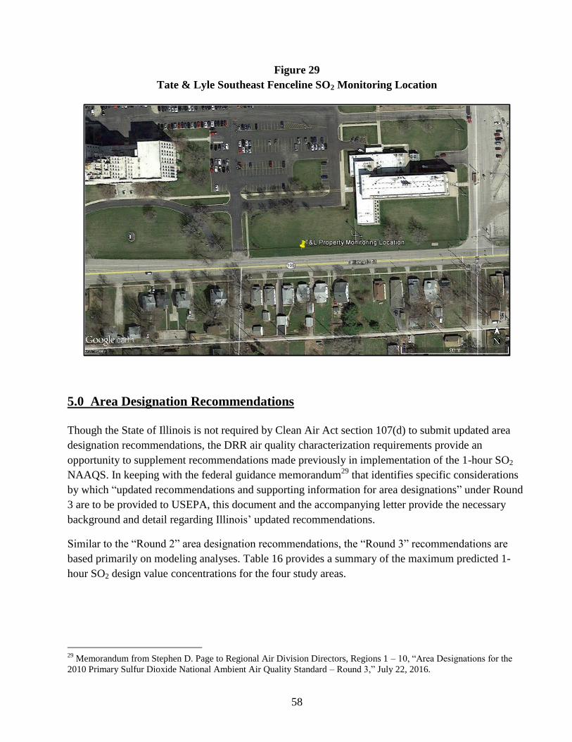
58
Figure 29
Tate & Lyle Southeast Fenceline SO2 Monitoring Location
5.0 Area Designation Recommendations
Though the State of Illinois is not required by Clean Air Act section 107(d) to submit updated area
designation recommendations, the DRR air quality characterization requirements provide an
opportunity to supplement recommendations made previously in implementation of the 1-hour SO2
NAAQS. In keeping with the federal guidance memorandum29
that identifies specific considerations
by which “updated recommendations and supporting information for area designations” under Round
3 are to be provided to USEPA, this document and the accompanying letter provide the necessary
background and detail regarding Illinois’ updated recommendations.
Similar to the “Round 2” area designation recommendations, the “Round 3” recommendations are
based primarily on modeling analyses. Table 16 provides a summary of the maximum predicted 1-
hour SO2 design value concentrations for the four study areas.
29
Memorandum from Stephen D. Page to Regional Air Division Directors, Regions 1 – 10, “Area Designations for the
2010 Primary Sulfur Dioxide National Ambient Air Quality Standard – Round 3,” July 22, 2016.

59
Table 16
Summary of the Four Study Areas
Maximum Predicted 99th
Percentile 1-Hour SO2 Design Value Concentration
Study Area Data Period
SO2 Concentration
(µg/m3)
Modeled NAAQS
Kincaid
2013 - 2015
64.28
196.32 Rain CII 105.01
Waukegan 98.91
Baldwin/Prairie State 78.21
The air quality characterization of the Kincaid Generation LLC electrical power generating station,
and vicinity, was a multi-county modeling analysis spanning large portions of Christian and
Sangamon counties and much lesser portions of Montgomery, Macoupin, and Macon counties.
Within the 45-kilometer radius study domain, only three SO2-emitting sources were considered to
have the potential for causing elevated impacts, either individually or through plume interaction. The
highest modeled 1-hour SO2 design value for these three sources, in combination with an ambient
background value, was less than one-third of the NAAQS. Given the widespread extent of low
modeled design values, the Illinois EPA is recommending attainment for the multi-county area of
Christian, Macoupin, Montgomery, and Sangamon counties.
The air quality characterization of the Rain CII Carbon facility and adjoining area in Crawford
County, Illinois, was undertaken using a 25-kilometer radius modeling domain that also encompassed
portions of neighboring Lawrence, Richland, Jasper, and Clark counties in Illinois and portions of
Sullivan and Knox counties in Indiana. Modeled impacts were determined only within Crawford
County and only from SO2-emitting processes at Rain CII Carbon, Marathon Petroleum Company,
and the Hoosier Energy – Merom Generating Station. The highest modeled 1-hour SO2 design value
for these three sources, in combination with an ambient background value, was slightly more than
one-half of the NAAQS. The Illinois EPA is recommending a designation of attainment of the 1-
hour SO2 standard for Crawford County.
The air quality characterization of the NRG Energy Inc. – Waukegan Station electrical power
generating plant and surrounding area involved modeling many more background sources than for
other study areas. The inclusion of these sources reflects the known local interest in air quality in
Lake County and the potential for combined elevated impacts from these sources. The land-based
portion of the 30-kilometer radius study domain consists mostly of eastern Lake County, a small
portion of Cook County, and a large portion of neighboring Kenosha County in Wisconsin. Modeled
impacts were generated for a large area of eastern Lake County, with the highest modeled 1-hour SO2
design value less than one-half of the NAAQS. The Illinois EPA recommends that all of Lake County
be designated as attainment for the 1-hour SO2 standard.

60
The air quality characterization of the area surrounding the Dynegy Midwest Generation – Baldwin
and Prairie State Generating Station power plants was a multi-county evaluation spanning large
portions of Randolph, Washington, and St. Clair counties, and much smaller portions of Perry,
Jackson, Clinton, Madison, and Monroe counties in Illinois, and Ste. Genevieve and Perry counties in
Missouri. Within the 50-kilometer radius study domain, two background sources in proximity to the
power plants were modeled. The inclusion of these sources provided reasonable assurance of capture
of potential maximum near-field impacts. The highest modeled 1-hour SO2 design value for all four
sources, in combination with an ambient background value, was less than one-half of the NAAQS.
Given the widespread extent of low modeled design values, the Illinois EPA recommends that
Monroe, Randolph, St. Clair, Perry, and Washington counties be designated as attainment for the 1-
hour SO2 standard.

61
Appendices

62
Appendix A
Emission Inventories for the Study Areas

63
Kincaid Study Area Emission Inventory
AERMOD Source
Description
Receptor Location
(Meters)
Stack
Height
Temperature and
Exit Velocity
Stack
Diameter
Emissions
Profile
Source ID East North (m) (K and m/s) (m)
0001KC
Stack 0001 -
Auxiliary Boiler
Stack (Gas Fired
Kincaid)
285670.58 4385485.58 41.15 See Hourly File 1.22 A
0007KC
Stack 0007 - Unit
1/Unit 2 Main
Stack (Boiler Unit
1-Kincaid)
285609.63 4385297.00 186.84 See Hourly File 9.02 A
0001CPP
Boiler #4 Stack
(Rain Cap) (CPP) -
Gas Fired
272584.10 4409442.21 22.86 See Hourly File 1.22 B
0002CPP
Boilers #1 #2 and
#3 Stack (CPP) -
Coal Fired
272538.09 4409435.07 50.29 See Hourly File 1.92 B
0006CPP
Boiler #5 Stack
(Rain Cap) (CPP) -
Gas Fired
272583.75 4409433.06 22.86 See Hourly File 1.22 B
0005CWLP Units 31/32 Stack
(CWLP) 277154.75 4403721.32 137.16 See Hourly File 3.96 A
0009CWLP Dallman 3 Unit 33
Stack (CWLP) 277047.97 4403790.25 152.40 See Hourly File 5.03 A
0017CWLP Dallman 4 Stack
(CWLP) 276830.83 4403754.28 137.16 See Hourly File 4.57 A
A: CEMS data, hourly varying emissions, temperature, exit velocity.
B: Hourly Profile of emissions based on three years of daily emissions, a constant used for temperature and exit velocity

64
Rain CII Carbon Study Area Emission Inventory
AERMOD Source
Description
Receptor Location
(Meters) Stack
Height
Temperature
and Exit
Velocity
Stack
Diameter
Emissions
Profile
Source ID East North (m) (K and m/s) (m)
0001RCII Pyroscrubber #1
Stack 437642.68 4315969.54 45.72
See Hourly
File 3.05 A
0003RCII Pyroscrubber #2
Stack 437639.42 4315893.11 45.72
See Hourly
File 3.05 A
MEROM_1 Unit 1 & 2 Stack
(Merom) 455758.5 4324641.70 214.58
See Hourly
File 5.79 B
MEROM_2
Unit 1 & 2 Stack
(Merom) 455765.5 4324641.40 214.58 See Hourly
File 5.79 B
HTR_1F1
Atmospheric
Heater 1F1
(Marathon) 437504.23 4316843.68 55.78
See Hourly
File 3.66 B
HTR_1F2
Vacuum
Distillation Heater
1F2 437464.99 4316834.33 57.91
See Hourly
File 2.24 C
HTR_2F1 Reactor Heater 2F1 437420.03 4316847.93 38.10
See Hourly
File 1.04 C
HTR_2F2 Stripper Reboiler
2F2 437400.68 4316849.62 39.62
See Hourly
File 1.47 C
HTR_3F1 Reactor Preheaters
3F1 437422.97 4316691.16 63.09
See Hourly
File 3.86 C
HTR_3F2 Reactor Preheaters
3F2 437422.97 4316691.16 63.09
See Hourly
File 3.86 C
HTR_3F3 Reactor Preheaters
3F3 437422.00 4316680.87 46.63
See Hourly
File 2.79 C
HTR_3F4 Reactor Preheaters
3F4 437422.00 4316680.87 46.63
See Hourly
File 2.79 C
HTR_3F7 Ultraformer Regen.
Heater 3F7 437392.76 4316700.60 30.48
See Hourly
File 0.91 C
HTR_4F1 Hydrotreater
Reactor Heater 4F1 437350.90 4316850.43 38.10
See Hourly
File 1.42 C
HTR_4F2 Hydrocracker
Reactor Heater 4F2 437350.60 4316843.46 38.100
See Hourly
File 1.42 C
HTR_4F3 Splitter Reboiler
4F3 437350.90 4316836.48 37.790
See Hourly
File 1.60 C
HTR_4F4 Debutanizer
Reboiler 4F4 437351.21 4316828.59 38.100
See Hourly
File 1.60 C
HTR_7F1 HF Alkyl.
Isostripper Reb.
7F1
437153.20 4316860.94 42.977 See Hourly
File 2.74 C
HTR_8F1 Debutanizer
Reboiler 8F1 437128.74 4316648.29 38.100
See Hourly
File 1.52 C
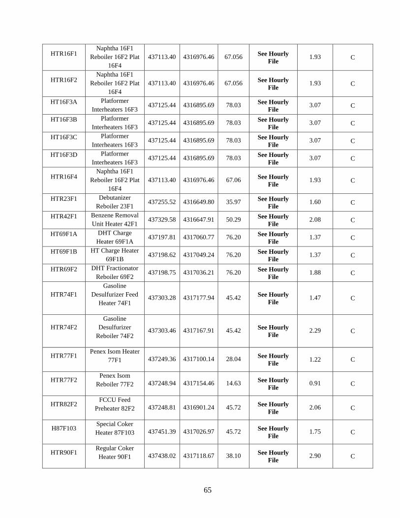
65
HTR16F1 Naphtha 16F1
Reboiler 16F2 Plat
16F4
437113.40 4316976.46 67.056 See Hourly
File 1.93 C
HTR16F2 Naphtha 16F1
Reboiler 16F2 Plat
16F4
437113.40 4316976.46 67.056 See Hourly
File 1.93 C
HT16F3A Platformer
Interheaters 16F3 437125.44 4316895.69 78.03
See Hourly
File 3.07 C
HT16F3B Platformer
Interheaters 16F3 437125.44 4316895.69 78.03
See Hourly
File 3.07 C
HT16F3C Platformer
Interheaters 16F3 437125.44 4316895.69 78.03
See Hourly
File 3.07 C
HT16F3D Platformer
Interheaters 16F3 437125.44 4316895.69 78.03
See Hourly
File 3.07 C
HTR16F4 Naphtha 16F1
Reboiler 16F2 Plat
16F4
437113.40 4316976.46 67.06 See Hourly
File 1.93 C
HTR23F1 Debutanizer
Reboiler 23F1 437255.52 4316649.80 35.97
See Hourly
File 1.60 C
HTR42F1 Benzene Removal
Unit Heater 42F1 437329.58 4316647.91 50.29
See Hourly
File 2.08 C
HT69F1A DHT Charge
Heater 69F1A 437197.81 4317060.77 76.20
See Hourly
File 1.37 C
HT69F1B HT Charge Heater
69F1B 437198.62 4317049.24 76.20
See Hourly
File 1.37 C
HTR69F2 DHT Fractionator
Reboiler 69F2 437198.75 4317036.21 76.20
See Hourly
File 1.88 C
HTR74F1
Gasoline
Desulfurizer Feed
Heater 74F1 437303.28 4317177.94 45.42
See Hourly
File 1.47 C
HTR74F2
Gasoline
Desulfurizer
Reboiler 74F2 437303.46 4317167.91 45.42
See Hourly
File 2.29 C
HTR77F1 Penex Isom Heater
77F1 437249.36 4317100.14 28.04 See Hourly
File 1.22 C
HTR77F2 Penex Isom
Reboiler 77F2 437248.94 4317154.46 14.63 See Hourly
File 0.91 C
HTR82F2 FCCU Feed
Preheater 82F2 437248.81 4316901.24 45.72 See Hourly
File 2.06 C
H87F103 Special Coker
Heater 87F103 437451.39 4317026.97 45.72 See Hourly
File 1.75 C
HTR90F1 Regular Coker
Heater 90F1 437438.02 4317118.67 38.10 See Hourly
File 2.90 C
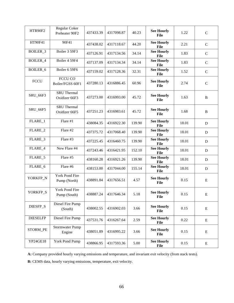
66
HTR90F2 Regular Coker
Preheater 90F2 437433.39 4317098.87 40.23 See Hourly
File 1.22 C
HT90F41 90F41 437438.02 4317118.67 44.20
See Hourly
File 2.21 C
BOILER_3 Boiler 3 59F3 437126.91 4317134.56 34.14
See Hourly
File 1.83 C
BOILER_4 Boiler 4 59F4 437137.09 4317134.34 34.14
See Hourly
File 1.83 C
BOILER_6 Boiler 6 59F6 437159.02 4317128.36 32.31
See Hourly
File 1.52 C
FCCU FCCU CO
Boiler/FGSS 60F1 437280.13 4316886.45 60.96 See Hourly
File 2.74 C
SRU_66F3 SRU Thermal
Oxidizer 66F3 437273.00 4316993.00 45.72 See Hourly
File 1.63 B
SRU_66F5 SRU Thermal
Oxidizer 66F5 437251.23 4316983.61 45.72 See Hourly
File 1.68 B
FLARE_1 Flare #1 438084.35 4316922.30 139.90
See Hourly
File 18.01 D
FLARE_2 Flare #2 437375.72 4317068.40 139.90
See Hourly
File 18.01 D
FLARE_3 Flare #3 437225.45 4316460.75 139.90
See Hourly
File 18.01 D
FLARE_4 New Flare #4 437243.46 4316421.95 152.10
See Hourly
File 18.01 D
FLARE_5 Flare #5 438160.28 4316921.26 139.90
See Hourly
File 18.01 D
FLARE_6 Flare #6 438153.00 4317044.00 155.14
See Hourly
File 18.01 D
YORKFP_N York Pond Fire
Pump (North) 438891.84 4317656.51 4.57 See Hourly
File 0.15 E
YORKFP_S York Pond Fire
Pump (South) 438887.24 4317646.34 5.18 See Hourly
File 0.15 E
DIESFP_S Diesel Fire Pump
(South) 438002.55 4316902.03 3.66 See Hourly
File 0.15 E
DIESELFP Diesel Fire Pump 437531.76 4316267.64 2.59
See Hourly
File 0.22 E
STORM_PE Stormwater Pump
Engine 438051.89 4316995.22 3.66 See Hourly
File 0.15 E
YP24GE18 York Pond Pump 438866.95 4317593.36 5.00
See Hourly
File 0.15 E
A: Company provided hourly varying emissions and temperature, and invariant exit velocity (from stack tests).
B: CEMS data, hourly varying emissions, temperature, exit velocity.

67
C: Derived from hourly heat input rates in combination with fuel gas emission factors (determined from continuous
emission monitoring of H2S in refinery fuel gas) provided the basis of the hourly emissions.
D: SO2 emission estimates for flaring reflect the H2S content of the gases flared and the quantity of gas being flared.
E: Day-specific operational data were provided for the stationary engines (fire pumps) at Marathon, and together with
SO2 emission rates developed from stack testing data and horsepower ratings, a particular engine’s emissions were
allocated uniformly across all hours of each specific day of operation.

68
Waukegan Study Area Emission Inventory
AERMOD Source Description
Receptor Location
(Meters) Stack
Height
Temperature
and Exit
Velocity
Stack
Diameter
Emissions
Profile
Source ID East North (m) (K and m/s) (m) (g/s)
0018WAU Waukegan Power
Unit #8 430011.73 4692529.25 137.16
See Hourly
File 4.1 A
0021WAU Waukegan Power
Unit #7 433012.39 4692584.59 137.16
See Hourly
File 4.3 A
0020WAU Peaker Stack 1 of 4 432761.42 4692481.37 13.11 672.0/21.64 3.3 B
0069WAU Peaker Stack 2 of 4 432762.09 4692508.58 13.11 672.0/21.64 3.3 B
0070WAU Peaker Stack 3 of 4 432788.52 4692508.27 13.11 672.0/21.64 3.2 B
0071WAU Peaker Stack 4 of 4 432787.89 4692481.06 13.11 672.0/21.64 3.3 B
PP_01 Pleasant Prairie Unit
1/2 Stack 425857.0 4709911.0 137.200
See Hourly
File 3.50 A
PP_02 Pleasant Prairie Unit
1/2 Stack 425857.0 4709910.0 137.200
See Hourly
File 3.50 A
0123ABBV Biogas flare (Abbvie,
Inc.) 431272.7 4687130.2 13.4627 1273.0/20.0 0.68 B
0086ABL Boiler #4AP (Abbott
Labs) 425854.3 4683793.7 32.949 428.7/8.07 1.83 B
0087ABL Boiler #5AP (Abbott
Labs) 425849.5 4683800.9 32.949 424.8/8.19 1.83 B
0006ABL Boiler #6AP (Abbott
Labs) 425858.05 4683791.54 21.708 505.4/7.92 1.22 C
0063ABL Boiler #7AP 9abbott
Labs) 425831.27 4683824.28 210.976 422.0/7.81 1.22 C
0001AD
Landfill Gas Flare
Enclosed Stack -
(Adv Disposal
Services Zion)
427387.1 4703452.0 18.290 1273.0/20/0 3.96 B
0003CG Turbine #1 Stack
(Countryside Genco) 414962.4 4685957.6 14.940 699.8/17.0 1.00 B
0004CG Turbine #2 Stack
(Countryside Genco) 414962.5 4685963.0 14.940 699.8/17.0 1.00 B
0005CG Turbine #3 Stack
(Countryside Genco) 414962.5 4685968.6 14.940 699.8/17.0 1.00 B
0006CG Turbine #4 Stack
(Countryside Genco) 414962.5 4685974.3 14.940 699.8/17.0 1.00 B
0001CL
Callidus Enclosed
Flare (Countryside
Landfill)
415403.8 4685577.3 13.720 1273.0/20/0 3.81 B
0007CL
Parnel Enclosed Flare
(Countryside
Landfill)
415432.5 4685586.4 15.240 1273.0/20.0 3.81 B
0001BE Engine #1 Stack (Bio
Energy Illinois LLC) 427390.6 4703495.5 9.997 738.15/26.5 0.36 B
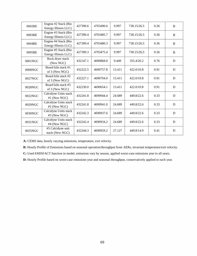
69
0002BE Engine #2 Stack (Bio
Energy Illinois LLC) 427390.6 4703490.6 9.997 738.15/26.5 0.36 B
0003BE Engine #3 Stack (Bio
Energy Illinois LLC) 427390.4 4703485.7 9.997 738.15/26.5 0.36 B
0004BE Engine #4 Stack (Bio
Energy Illinois LLC) 427390.4 4703480.3 9.997 738.15/26.5 0.36 B
0005BE Engine #5 Stack (Bio
Energy Illinois LLC) 427390.3 4703475.4 9.997 738.15/26,5 0.36 B
0001NGC Rock dryer stack
(New NGC) 432147.1 4690868.0 9.449 355.4/20.2 0.76 D
0008NGC Board kiln stack #1
of 3 (New NGC) 432222.5 4690757.8 13.411 422.0/10.8 0.91 D
0027NGC Board kiln stack #2
of 3 (New NGC) 432227.1 4690704.0 13.411 422.0/10.8 0.91 D
0028NGC Board kiln stack #3
of 3 (New NGC) 432230.0 4690654.1 13.411 422.0/10.8 0.91 D
0022NGC Calcidyne Units stack
#1 (New NGC) 432241.8 4690944.4 24.689 449.8/22.6 0.33 D
0029NGC Calcidyne Units stack
#2 (New NGC) 432241.8 4690941.0 24.689 449.8/22.6 0.33 D
0030NGC Calcidyne Units stack
#3 (New NGC) 432242.3 4690937.6 24.689 449.8/22.6 0.33 D
0031NGC Calcidyne Units stack
#4 (New NGC) 432242.4 4690934.2 24.689 449.8/22.6 0.33 D
0025NGC #5 Calcidyne unit
stack (New NGC) 432244.3 4690929.2 27.127 449.8/14.9 0.41 D
A: CEMS data, hourly varying emissions, temperature, exit velocity.
B: Hourly Profile of Emissions based on seasonal operation/throughput from AERs, invariant temperature/exit velocity.
C: Used EMISFACT function in model, emissions vary by season, applied worst-case emissions year to all years.
D: Hourly Profile based on worst-case emissions year and seasonal throughput, conservatively applied to each year.

70
Baldwin/Prairie State Generating Study Area Emission Inventory
AERMOD Source
Description
Receptor Location
(Meters) Stack
Height
Temperature
and Exit
Velocity
Stack
Diameter
Emissions
Profile
Source ID East North (m) (K and m/s) (m) (g/s)
0001BD Boiler #1
(Baldwin) 249934.19 4232425.13 184.40
See Hourly
File 5.94 A
0002BD Boiler #2
(Baldwin) 249931.24 4232363.94 184.40
See Hourly
File 5.94 A
0013BD Boiler #3
(Baldwin) 249928.04 4232301.51 184.40
See Hourly
File 5.94 A
0005BD Heating Boiler
(Baldwin) 250017.08 423244.00 84.12
See Hourly
File 1.07 B
0004PS EP10A Boiler #1
(Prairie St.) 266714.30 4240167.70 213.36
See Hourly
File 8.53 A
0006PS EP10A Boiler # 2
(Prairie St.) 266725.10 4240167.30 213.36
See Hourly
File 8.53 A
0006USM
ROTARY DRYER
#4 FUEL OIL
COMBUSTION
(US Minerals)
250168.25 4231328.50 7.62 See Hourly
File 2.19 C
0002CH Flare
(Cottonwood) 256967.25 4238205.70 17.75
See Hourly
File 2.43 C
0005PS Auxiliary Boiler
(Prairie St.) 266583.30 4239848.58 30.48 425.00/20.00 1.52 D
0004CH Crusher
(Cottonwood) 256530.90 4238479.80 6.10 493.71/19.22 0.46 D
A: CEMS data, hourly varying emissions, temperature, exit velocity.
B: Hourly emissions profile based on data provided by company from monthly fuel usage and monthly operating hours.
C: Hourly Profile of emissions based on seasonal operation/throughput from AERs.
D: Hourly Profile based on worst-case emissions year and seasonal throughput, conservatively applied to each year.

71
Appendix B
Background SO2 Data for Modeling

72
Nilwood*, Illinois Monitor
Seasonally**
and Hourly Varying Background SO2
Kincaid & Rain CII Carbon Study Areas
Hour of Day
SO2 Concentration (µg/m3)
Winter Spring Summer Fall
1 7.68 5.58 5.41 5.41
2 7.50 4.80 5.93 5.50
3 7.68 4.54 4.19 6.37
4 6.89 5.58 6.11 5.32
5 7.68 4.54 5.24 6.28
6 7.59 5.76 6.46 6.37
7 7.59 5.32 6.89 6.28
8 7.50 8.38 8.90 6.81
9 9.07 10.91 9.16 9.77
10 14.75 10.73 9.42 9.16
11 15.44 13.70 10.82 12.65
12 15.09 12.56 9.42 12.56
13 14.13 11.60 7.68 11.78
14 13.52 10.30 8.46 9.51
15 13.52 9.51 8.55 8.46
16 12.04 9.07 6.19 8.64
17 11.43 7.33 5.85 7.77
18 10.12 6.72 5.24 6.72
19 8.20 6.54 4.97 6.72
20 9.51 4.80 4.97 6.37
21 9.60 5.32 4.89 6.46
22 7.85 5.06 4.10 7.15
23 7.50 4.36 4.10 6.54
24 7.68 4.36 4.80 5.93
* Monitor Latitude/Longitude Coordinates: (+39.396075 –89.80974)
** Seasons defined as: Winter (Dec, Jan, Feb), Spring (Mar, Apr, May), Summer (Jun, Jul, Aug), Fall (Sep, Oct, Nov)

73
Oglesby*, Illinois Monitor
Seasonally**
and Hourly Varying Background SO2
Waukegan Study Area
Hour of Day
SO2 Concentration (µg/m3)
Winter Spring Summer Fall
1 5.76 6.63 4.62 5.85
2 6.46 8.03 5.06 5.24
3 5.24 8.20 3.32 4.45
4 5.76 6.72 2.44 4.80
5 6.72 5.76 1.92 7.15
6 6.98 7.15 2.27 7.85
7 6.46 6.28 4.10 6.11
8 7.85 8.46 8.03 5.50
9 9.69 10.91 10.47 6.19
10 12.22 11.52 10.56 9.77
11 12.74 11.95 10.21 11.78
12 14.13 12.91 6.72 10.30
13 15.09 9.95 7.68 8.20
14 15.01 9.95 7.50 8.38
15 12.22 8.03 6.46 7.50
16 11.26 7.24 5.85 6.98
17 10.64 8.46 6.37 7.33
18 9.95 7.42 6.37 7.24
19 9.25 9.77 7.59 4.71
20 8.29 7.85 4.62 7.33
21 8.81 9.16 4.28 7.68
22 7.15 10.38 4.97 6.89
23 6.72 8.20 4.97 4.97
24 6.54 6.72 3.93 5.50
* Monitor Latitude/Longitude Coordinates: (+41.29301 -89.04942)
** Seasons defined as: Winter (Dec, Jan, Feb), Spring (Mar, Apr, May), Summer (Jun, Jul, Aug), Fall (Sep, Oct, Nov)

74
East St. Louis*, Illinois Monitor
Seasonally**
and Hourly Varying Background SO2
Baldwin/Prairie State Generating Station
Hour of Day
SO2 Concentration (µg/m3)
Winter Spring Summer Fall
1 21.73 14.57 7.50 10.56
2 17.28 11.87 18.32 11.08
3 9.60 13.26 17.63 14.40
4 11.26 17.36 12.91 12.13
5 12.13 22.34 13.79 11.43
6 10.38 13.44 10.30 9.25
7 9.60 17.71 11.69 11.43
8 12.83 15.53 19.98 21.81
9 14.48 16.93 31.85 22.95
10 19.98 23.12 27.05 34.29
11 28.53 27.75 24.78 25.83
12 23.03 19.54 19.54 19.89
13 31.32 16.40 18.67 16.23
14 24.26 15.97 17.10 19.98
15 19.02 16.75 15.01 15.71
16 18.15 13.79 17.71 14.22
17 17.89 17.63 12.91 13.79
18 18.06 14.40 13.52 14.57
19 15.71 14.57 10.64 12.48
20 10.38 12.22 9.51 9.16
21 10.56 10.47 14.57 7.07
22 14.83 9.51 9.34 9.86
23 17.54 9.95 8.29 7.24
24 28.10 13.87 8.81 7.94
* Monitor Latitude/Longitude Coordinates: (+38.61203 -90.16048)
** Seasons defined as: Winter (Dec, Jan, Feb), Spring (Mar, Apr, May), Summer (Jun, Jul, Aug), Fall (Sep, Oct, Nov)