Embed Size (px)
Citation preview
Data Mining to Improve Traffic Safety
By
Randy K. Smith and Huanjing Wang
Department of Computer Science, The University of Alabama,
Box 870290, Tuscaloosa, AL 35487-0290
Prepared by
UTCA University Transportation Center for Alabama
The University of Alabama, The University of Alabama in Birmingham, and The University of Alabama at Huntsville
UTCA Report 04107
May 26, 2005

ii
iii
Technical Report Documentation Page
1. Report No
2. Government Accession No. 3. Recipient Catalog No.
5. Report Date May 26, 2005
4. Title and Subtitle Data Mining to Improve Traffic Safety 6. Performing Organization Code
7. Authors Dr. Randy K. Smith and Ms. Huanjing Wang
8. Performing Organization Report No. UTCA 04107
10. Work Unit No.
9. Performing Organization Name and Address University Transportation Center for Alabama P O Box 870205 University of Alabama Tuscaloosa, AL 35487-0205
11. Contract or Grant No. DTSR0023424
13. Type of Report and Period Covered Final Report: 01/01/2004 – 12/31/2004
12. Sponsoring Agency Name and Address University Transportation Center for Alabama P O Box 870205 University of Alabama Tuscaloosa, AL 35487-0205
14. Sponsoring Agency Code
15. Supplementary Notes 16. Abstract The ever increasing size of datasets used for data mining and machine learning applications has placed a renewed emphasis on algorithm performance and processing strategies. This research addresses algorithms for ranking variables in a dataset, as well as for ranking values of a specific variable. We propose two new techniques, called Max Gain (MG) and Sum Max Gain Ratio (SMGR), which are well-correlated with existing techniques, yet are much more intuitive. MG and SMGR were developed for the public safety domain using categorical traffic accident data. Unlike the typical abstract statistical techniques for ranking variables and values, the proposed techniques can be motivated as useful intuitive metrics for non-statistician practitioners in a particular domain. Additionally, the developed techniques are generally more efficient than the more traditional statistical approaches. 17. Key Words Data mining, traffic safety
18. Distribution Statement
19. Security Class (of report)
20. Security Class. (Of page)
21. No of Pages
22. Price
iv
Contents
Contents ............................................................................................................................ iii Tables................................................................................................................................ v Figures............................................................................................................................... v Executive Summary............................................................................................................ vi
1.0 Introduction............................................................................................................. 1 Value and Variable Ranking ................................................................................... 2
2.0 The Problem Domain............................................................................................... 4 Traffic Accident Analysis........................................................................................ 4
3.0 Value Ranking......................................................................................................... 6 Value Ranking Fundamentals.................................................................................. 6 Existing Value Ranking Methods............................................................................. 7
Statistical Significance Z Value (SSZ) ......................................................... 7 Confidence (CF) and Support (SP) ............................................................ 7 Improvement (IM) ..................................................................................... 8
4.0 New Value Ranking Methods.................................................................................. 9
New Value Ranking Techniques............................................................................. 9 Over-Representation (OR)......................................................................... 9 Max Gain (MG)......................................................................................... 9 Max-Max Gain (MMG)............................................................................. 11
Results Using New Value Ranking Method............................................................. 12 Pearson’s Correlation With Existing Methods ............................................. 12 Running Time Efficiency Compared With Existing Techniques...................... 12
5.0 Variable Ranking..................................................................................................... 14
The Variable Ranking Problem............................................................................... 14 Existing Variable Ranking Methods......................................................................... 14
Chi-squared (CHI)..................................................................................... 14 Correlation Coefficient (CC)...................................................................... 15 Information Gain (IG)................................................................................. 15 Gain Ratio (GR)......................................................................................... 16
v
6.0 A New Variable Ranking Method............................................................................ 17 Sum Max Gain Ratio (SMGR) ............................................................................... 17 Results Using SMGR ............................................................................................. 18
Pearson’s Correlation With Existing Methods ............................................. 19 Running Time Comparison.......................................................................... 20 Classification.............................................................................................. 20
7.0 Using column-major storage to improve variable selection performance .................... 22
Motivation............................................................................................................. 22 Results Under Value Ranking ................................................................................. 22 Results Under Variable Ranking ............................................................................. 23
8.0 Integration with CARE ............................................................................................ 28 8.1 Improved Query Interface............................................................................... 28
9.0 Conclusions............................................................................................................. 32
10.0 References............................................................................................................. 33
vi
List of Tables
Number Page 3-1 A contingency table of variable Vk and target variable ...........................................3 4-1 An example of Max Gain....................................................................................10 4-2 An example of Max-Max Gain...........................................................................11 4-3 Number of variables correlated to MG ...............................................................13 4-4 Comparison of run times for different value ranking techniques (in milliseconds).................................................................................13 6-1 Frequency table of variable of “Day of Week”....................................................18 6-2 Pearson’s correlation, SMGR and other methods................................................19 6-3 Complexity analysis............................................................................................19 6-4 Comparison of run times for different variable ranking techniques (in milliseconds).................................................................................20 6-5 Results for the C4.5 algorithm.............................................................................21 7-1 Variable selection, row-major order ...................................................................26 7-2 Variable selection, column-major order...............................................................27 8-1 Description of featured elements in Figure 8-1.....................................................29 8-2 Summary of top five variables from Figure 8-1....................................................29 8-3 Summary of top five variables from Figure 8-2....................................................30 8-4 Summary of top five variables from Figure 8-3....................................................31
List of Figures
Number Page
1-1 The data mining process.......................................................................................2 7-1 Average value ranking performance, column-major versus row-major .................23 7-2 Performance comparison, row-major versus column-major, fixed number of rows, SMGR.............................................................................24 7-3 Performance comparison, row-major versus column-major, fixed columns, SMGR. .......................................................................................25 8-1 Alcohol related filter, rank by SMGR..................................................................28 8-2 Alcohol related filter, rank by CC ......................................................................30 8-3 Alcohol related filter, rank by CHI......................................................................31

vii
Executive Summary
The ever increasing size of datasets used for data mining and machine learning applications has placed a renewed emphasis on algorithm performance and processing strategies. This research addresses algorithms for ranking variables in a dataset, as well as for ranking values of a specific variable. We propose two new techniques, called Max Gain (MG) and Sum Max Gain Ratio (SMGR), which are well-correlated with existing techniques, yet are much more intuitive. MG and SMGR were developed for the public safety domain using categorical traffic accident data. Unlike the typical abstract statistical techniques for ranking variables and values, the proposed techniques can be motivated as useful intuitive metrics for non-statistician practitioners in a particular domain. Additionally, the developed techniques are generally more efficient than the more traditional statistical approaches
1
Section 1 Introduction
Motivation Data mining is the exploration and analysis of a large dataset in order to discover knowledge and rules. Data mining has been very successful as a technique for deriving new information in a variety of domains (Berry & Linoff, 1997). Data mining is typically conceptualized as a three-part process: preprocessing, learning (or training) and post-processing. In the last decade, data that serves as a target for data mining has grown explosively. Data has been growing increasingly larger in both the number of rows (i.e., records) and columns (i.e., variables). The quality of data affects the success of data mining on a given learning task. If information is irrelevant or noisy, then knowledge discovery during training time can be ineffective (Hall & Smith, 1999). Variable selection is a process of keeping only useful variables and removing irrelevant and noisy information. It is always used as a data mining preprocessing step, particularly for high-dimensional data.
Variable selection can be used to select subsets of variables in terms of predictive power. Since variable selection effectively ranks set of variables according to importance, it may be referred to as variable ranking. There is also an analogous notion of value ranking, which refers to the idea of ranking the values of a particular variable in terms of their relative importance. In this research, we examine existing techniques for both variable and value ranking, and we propose new techniques in both categories. Our techniques were developed from traffic accident data utilized by public safety officials searching for efficient mechanisms to identify, develop and deploy appropriate countermeasures and enforcement regiments to lower traffic accident occurrences. We show that our proposed techniques give similar results to existing techniques, yet are conceptually simpler, and therefore of greater value to a practitioner using data mining in a particular domain. In particular, the proposed techniques are metrics that are meaningful to a practitioner beyond just their statistical implications. Because our proposed techniques are also relatively efficient, they can be used efficiently as conceptually simple substitutes for the more traditional and complex statistical approaches.
As a further investigation of the efficiency of our proposed techniques, we examine their performance under competing storage models. We show that when data are stored in column-major order, the performance of our proposed techniques is quite favorable. While column-major order is generally inappropriate for transactional systems, it has been shown to be superior to row-major order for non-transactional, statistical analysis systems that utilize categorical data (Parrish et al., 2005). Our
2
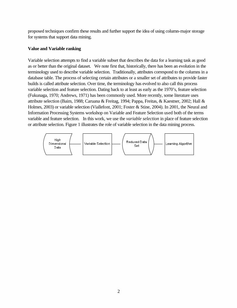
proposed techniques confirm these results and further support the idea of using column-major storage for systems that support data mining. Value and Variable ranking Variable selection attempts to find a variable subset that describes the data for a learning task as good as or better than the original dataset. We note first that, historically, there has been an evolution in the terminology used to describe variable selection. Traditionally, attributes correspond to the columns in a database table. The process of selecting certain attributes or a smaller set of attributes to provide faster builds is called attribute selection. Over time, the terminology has evolved to also call this process variable selection and feature selection. Dating back to at least as early as the 1970’s, feature selection (Fukunaga, 1970; Andrews, 1971) has been commonly used. More recently, some literature uses attribute selection (Baim, 1988; Caruana & Freitag, 1994; Pappa, Freitas, & Kaestner, 2002; Hall & Holmes, 2003) or variable selection (Viallefont, 2001; Foster & Stine, 2004). In 2001, the Neural and Information Processing Systems workshop on Variable and Feature Selection used both of the terms variable and feature selection. In this work, we use the variable selection in place of feature selection or attribute selection. Figure 1 illustrates the role of variable selection in the data mining process.
Figure 1-1. The data mining process
In data mining, variable selection generally falls into two categories (Kohavi, John, & Pfleger, 1994; Mladenic & Grobelnik, 1999): § The filter model and § The wrapper model.
The filter model selects a variable subset independently without involving any learning algorithm that will use the selected variables. The wrapper model selects a variable subset using the evaluation function based on the predetermined learning algorithm. This type of wrapper approach generally produces a better variable subset but tends to consume a lot of resources. When the number of variables is very large, filtering is generally the preferred approach. As noted above, one filter model technique is commonly referred to as variable ranking (Kohavi & John, 1997; Guyon & Elisseeff, 2003). Variable ranking is a data mining preprocessing step where variables are selected independently of the learning algorithm that will use the selected variables. The procedure of variable ranking is to score each variable according to a particular method; the best k variables will then be selected. For example, using a given method, rank the 10 best variables in predicting alcohol related traffic accidents. The advantage of variable ranking is that it requires only the

3
computation of scores of each variable individually and sorting the scores (Guyon & Elisseeff, 2003; Stoppiglia et al., 2003). Also as noted above, value ranking is closely akin to variable ranking. For categorical data, a variable may take on one of a fixed set of possible values. For example, a variable labeled gender may take on values of “Male,” “Female,” or “Unknown.” Value ranking is the process of determining what values of a variable are most important or contribute most significantly to the variable selection process. For example, if the variable “Gender” is ranked significant in predicting alcohol related accidents, the value “Male” can be seen as the most important contributor in “Gender” being ranked. Our approach in this research is to examine existing value and variable ranking techniques. We then propose new techniques that represent metrics that have intuitive utility to a practitioner, comparing our proposed techniques to the existing ones in terms of (a) consistency with the existing techniques and (b) performance. We show that the proposed techniques correlate well with the existing techniques, with favorable performance as well. Value and variable ranking are statistical approaches that examine one or a small number of attributes that describe a record. Traditionally, these attributes are considered to be the columns in a two dimensional table with each record being a row in the table. Previous results indicate that statistical operations such as frequency and cross-tabulations are more efficient when the underlying data is stored and processed in column-major order (i.e., with each column stored contiguously on the disk) (Parrish et al., 2005). This is contrary to the vast majority of contemporary database systems that process their data in row-major order (i.e., with each row stored contiguously on the disk). In particular, rows are often inserted or deleted as a unit and updates tend to be row-oriented. Statistical processing which may be concerned with only a few attributes (columns) benefits from column-major order. Our results in evaluating Max Gain (MG), a new value ranking technique that we propose, and Sum Max Gain Ratio (SMGR), a new variable ranking technique that we propose, continue to support this research.
4
Section 2 The Problem Domain
Traffic Accident Analysis The particular problem domain addressed in this study is the analysis of automobile traffic accident data. Given the appropriate tools and data, variable ranking allows traffic safety professionals to develop and adopt countermeasures to reduce the volume and severity of traffic accidents (Parrish et al., 2003). The University of Alabama has developed a software system called CARE (Critical Analysis Reporting Environment) for the analysis of traffic crash data. CARE provides a tool that allows transportation safety engineers and policy makers to analyze the data collected from traffic accident records. CARE has been applied to traffic crash records from a number of states. The Alabama statewide crash database in CARE has records (rows) that contain 228 categorical variables (column); each variable contains attribute values varying from 2 to more than 600. CARE’s analysis domain is restricted to categorical data, represented by nominal, ordinal and interval based variables. Nominal variables have attribute values that have no natural order to them (e.g., pavement conditions – wet, dry, icy, etc.). Ordinal variables do have a natural order (e.g., number of injured, day of the week). Interval variables are created from intervals on a contiguous scale (e.g., age of driver – 16-20, 20-25, 25-35, etc.). The current system provides the users with filters to perform data analysis on particular subsets of the data that are of interest. Filters are defined by Boolean expressions over the variables in the database. A record satisfying a filter’s Boolean expression is a member of the filter subset, while a record not satisfying the filter’s Boolean expression is excluded from the filter subset. Common filters for crash data are filters for crashes within specific counties, filters defining crashes related to alcohol, filters defining crashes involving pedestrians, etc. In terms of our variable ranking techniques, the filter represents the target variable for learning with two values: “0” and “1.” In particular, “0” corresponds to the records not satisfying the filter’s Boolean expression, while “1” corresponds to the records satisfying the Boolean expression. Filters provide an effective conceptual framework for our value and variable ranking techniques in that they define two subsets: a control subset and an experimental subset. The idea that a filter defines an experimental group that is compared with a control group is fundamental to the value and variable ranking techniques discussed here. For example, in our traffic crash domain, an “alcohol” filter defines the subset of crashes where alcohol is involved. Our value and variable ranking techniques compare the alcohol crashes (experimental group) with all other crashes (control group) to conclude which values and variables are most important.
5
Section 3 Value Ranking
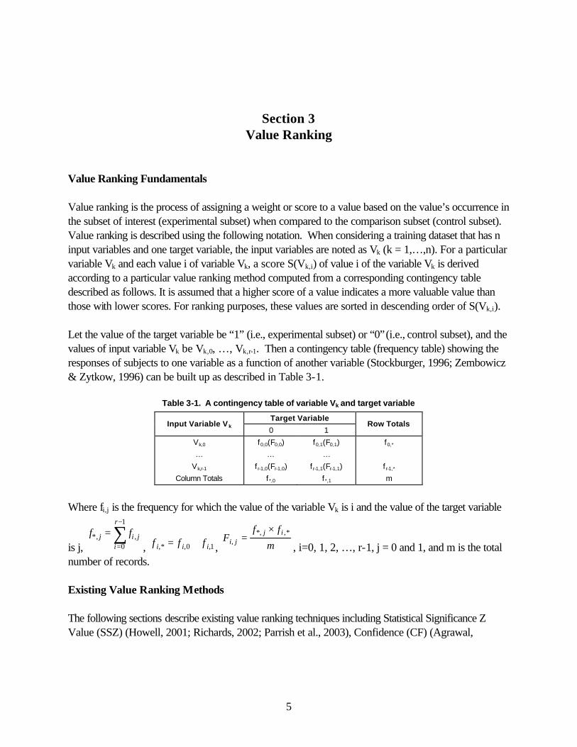
Value Ranking Fundamentals Value ranking is the process of assigning a weight or score to a value based on the value’s occurrence in the subset of interest (experimental subset) when compared to the comparison subset (control subset). Value ranking is described using the following notation. When considering a training dataset that has n input variables and one target variable, the input variables are noted as Vk (k = 1,…,n). For a particular variable Vk and each value i of variable Vk, a score S(Vk,i) of value i of the variable Vk is derived according to a particular value ranking method computed from a corresponding contingency table described as follows. It is assumed that a higher score of a value indicates a more valuable value than those with lower scores. For ranking purposes, these values are sorted in descending order of S(Vk,i). Let the value of the target variable be “1” (i.e., experimental subset) or “0” (i.e., control subset), and the values of input variable Vk be Vk,0, …, Vk,r-1. Then a contingency table (frequency table) showing the responses of subjects to one variable as a function of another variable (Stockburger, 1996; Zembowicz & Zytkow, 1996) can be built up as described in Table 3-1.
Table 3-1. A contingency table of variable Vk and target variable
Target Variable Input Variable V k
0 1 Row Totals
Vk,0 f0,0(F0,0) f0,1(F0,1) f0,*
… … …
Vk,r-1 f r-1,0(Fr-1,0) f r-1,1(Fr-1,1) f r-1,*
Column Totals f *,0 f *,1 m
Where fi,j is the frequency for which the value of the variable Vk is i and the value of the target variable
is j, ∑
−
=
=1
0,*,
r
ijij ff, 1,0,,* iii fff += , m
ffF
ijji
,**,,
×=
, i=0, 1, 2, …, r-1, j = 0 and 1, and m is the total number of records. Existing Value Ranking Methods The following sections describe existing value ranking techniques including Statistical Significance Z Value (SSZ) (Howell, 2001; Richards, 2002; Parrish et al., 2003), Confidence (CF) (Agrawal,
6
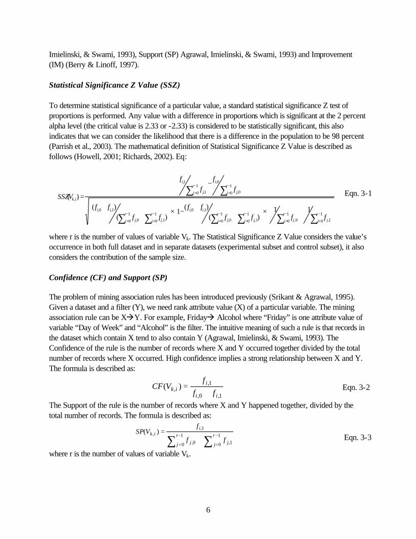
Imielinski, & Swami, 1993), Support (SP) Agrawal, Imielinski, & Swami, 1993) and Improvement (IM) (Berry & Linoff, 1997). Statistical Significance Z Value (SSZ) To determine statistical significance of a particular value, a standard statistical significance Z test of proportions is performed. Any value with a difference in proportions which is significant at the 2 percent alpha level (the critical value is 2.33 or -2.33) is considered to be statistically significant, this also indicates that we can consider the likelihood that there is a difference in the population to be 98 percent (Parrish et al., 2003). The mathematical definition of Statistical Significance Z Value is described as follows (Howell, 2001; Richards, 2002). Eq:
where r is the number of values of variable Vk. The Statistical Significance Z Value considers the value’s occurrence in both full dataset and in separate datasets (experimental subset and control subset), it also considers the contribution of the sample size. Confidence (CF) and Support (SP) The problem of mining association rules has been introduced previously (Srikant & Agrawal, 1995). Given a dataset and a filter (Y), we need rank attribute value (X) of a particular variable. The mining association rule can be XàY. For example, Fridayà Alcohol where “Friday” is one attribute value of variable “Day of Week” and “Alcohol” is the filter. The intuitive meaning of such a rule is that records in the dataset which contain X tend to also contain Y (Agrawal, Imielinski, & Swami, 1993). The Confidence of the rule is the number of records where X and Y occurred together divided by the total number of records where X occurred. High confidence implies a strong relationship between X and Y. The formula is described as:
1,0,
1,, )(
ii
iik ff
fVCF
+=
The Support of the rule is the number of records where X and Y happened together, divided by the total number of records. The formula is described as:
∑∑ −
=
−
=+
=1
0 1,1
0 0,
1,, )(
r
j jr
j j
iik
ff
fVSP
where r is the number of values of variable Vk.
+×
++
−×
++
−
=
∑∑∑∑∑∑
∑∑
−
=
−
=
−
=
−
=
−
=
−
=
−
=
−
=
1
0 1,1
0 0,1
0 1,1
0 0,
1,0,1
0 1,1
0 0,
1,0,
1
0 0,
0,1
0 1,
1,
,
11)(
)(1
)()(
)(
r
j jr
j jr
j jr
j j
iir
j jr
j j
ii
r
j j
ir
j j
i
ik
ffffff
ffff
ff
ff
VSSZ Eqn. 3-1
Eqn. 3-2
Eqn. 3-3
7
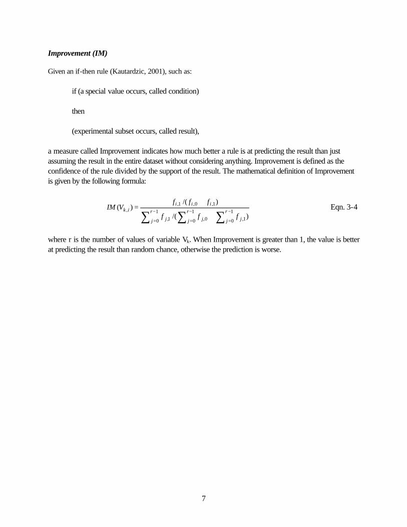
Improvement (IM) Given an if-then rule (Kautardzic, 2001), such as:
if (a special value occurs, called condition) then (experimental subset occurs, called result),
a measure called Improvement indicates how much better a rule is at predicting the result than just assuming the result in the entire dataset without considering anything. Improvement is defined as the confidence of the rule divided by the support of the result. The mathematical definition of Improvement is given by the following formula:
)/(
)/()(
1
0 1,1
0 0,1
0 1,
1,0,1,,
∑∑∑ −
=
−
=
−
=+
+=
r
j jr
j jr
j j
iiiik
fff
fffVIM
where r is the number of values of variable Vk. When Improvement is greater than 1, the value is better at predicting the result than random chance, otherwise the prediction is worse.
Eqn. 3-4

8
Section 4 New Value Ranking Methods
New Value Ranking Techniques As detailed above, value ranking is the process of assigning a weight or score to a value based on its occurrence in the experimental subset under investigation when compared to the control subset. We propose three value ranking techniques: Over-Representation (OR), MG, and Max-Max Gain (MMG). Over-Representation (OR) Over-Representation is a simple extension of a frequency distribution. The degree of Over-Representation for a particular value is the value’s occurrence in the experimental subset (the subset of interest) divided by the value’s occurrence in the control subset (the subset for the comparison purpose) (Parrish et al., 2003). To calculate the degree of Over-Representation for a particular value one must first determine the value’s occurrence in both the experimental class and control class (computed as percentage) and then divide these two values. It is possible to derive the Over-Represented values from a contingency table. Suppose variable Vk has value i, the Over-Representation of value i can be obtained by:
∑∑
−
=
−
==1
0 0,0,
1
0 1,1,
,/
/)(
r
j ji
r
j ji
ikff
ffVOR
where r is the number of values of variable Vk. Consider an example from the traffic safety domain. Suppose that 50 percent of the alcohol crashes occur on rural roadways, while only 25 percent of the non-alcohol crashes occur on rural roadways. Therefore, the degree of Over-Representation of alcohol crashes on rural roadways is 50 percent /25 percent = 2. Put simply, alcohol accidents are Over-Represented on rural roadways by a factor of 2. If the degree of Over-Representation is greater than 1, the value is an Over-Represented value. In the traffic safety domain, Over-Representation often indicates problems that need to be addressed through countermeasures (i.e., safety devices, sobriety checks, etc). As a simple ratio, OR is obviously a very intuitive quantity to a practitioner. Max Gain (MG) One important question a safety professional might ask is: What is the potential benefit from a proposed countermeasure? The answer to this question is that in the best case a countermeasure will reduce crashes to its expected value. It is unlikely to reduce crashes to a level less than what is found in the
Eqn. 4-1
9
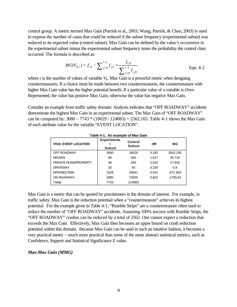
control group. A metric termed Max Gain (Parrish et al., 2003; Wang, Parrish, & Chen, 2003) is used to express the number of cases that could be reduced if the subset frequency (experimental subset) was reduced to its expected value (control subset). Max Gain can be defined by the value’s occurrence in the experimental subset minus the experimental subset frequency times the probability the control class occurred. The formula is described as:
∑∑
−
= −
=
×−=1
0 1
0 0,
0,1,1,, )(
r
j r
j j
ijiik
f
fffVMG
where r is the number of values of variable Vk. Max Gain is a powerful metric when designing countermeasures. If a choice must be made between two countermeasures, the countermeasure with higher Max Gain value has the higher potential benefit. If a particular value of a variable is Over-Represented, the value has positive Max Gain, otherwise the value has negative Max Gain. Consider an example from traffic safety domain: Analysis indicates that “OFF ROADWAY” accidents demonstrate the highest Max Gain in an experimental subset. The Max Gain of “OFF ROADWAY” can be computed by: 3680 – 7743 * (18029 / 124883) = 2562.165. Table 4-1 shows the Max Gain of each attribute value for the variable “EVENT LOCATION”.
Table 4-1. An example of Max Gain
V016: EVENT LOCATION Experimenta
l Subset
Control Subset
OR MG
OFF ROADWAY 3680 18029 3.292 2562.165
MEDIAN 89 940 1.527 30.718
PRIVATE ROAD/PROPERTY 46 293 2.532 27.833
DRIVEWAY 10 50 3.226 6.9
INTERSECTION 1028 30641 0.541 -871.804
ON ROADWAY 2890 74930 0.622 -1755.81
Totals 7743 124883
Max Gain is a metric that can be quoted by practitioners in the domain of interest. For example, in traffic safety, Max Gain is the reduction potential when a “countermeasure” achieves its highest potential. For the example given in Table 4-1, “Rumble Strips” are a countermeasure often used to reduce the number of “OFF ROADWAY” accidents. Assuming 100% success with Rumble Strips, the “OFF ROADWAY” crashes can be reduced by a total of 2562. One cannot expect a reduction that exceeds the Max Gain. Effectively, Max Gain then becomes an upper bound on crash reduction potential within this domain. Because Max Gain can be used in such an intuitive fashion, it becomes a very practical metric – much more practical than some of the more abstract statistical metrics, such as Confidence, Support and Statistical Significance Z value. Max-Max Gain (MMG)
Eqn. 4-2
10
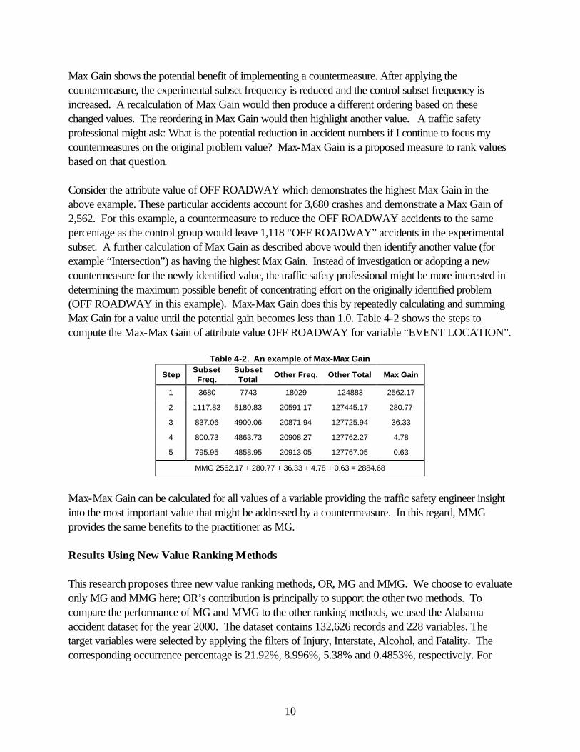
Max Gain shows the potential benefit of implementing a countermeasure. After applying the countermeasure, the experimental subset frequency is reduced and the control subset frequency is increased. A recalculation of Max Gain would then produce a different ordering based on these changed values. The reordering in Max Gain would then highlight another value. A traffic safety professional might ask: What is the potential reduction in accident numbers if I continue to focus my countermeasures on the original problem value? Max-Max Gain is a proposed measure to rank values based on that question. Consider the attribute value of OFF ROADWAY which demonstrates the highest Max Gain in the above example. These particular accidents account for 3,680 crashes and demonstrate a Max Gain of 2,562. For this example, a countermeasure to reduce the OFF ROADWAY accidents to the same percentage as the control group would leave 1,118 “OFF ROADWAY” accidents in the experimental subset. A further calculation of Max Gain as described above would then identify another value (for example “Intersection”) as having the highest Max Gain. Instead of investigation or adopting a new countermeasure for the newly identified value, the traffic safety professional might be more interested in determining the maximum possible benefit of concentrating effort on the originally identified problem (OFF ROADWAY in this example). Max-Max Gain does this by repeatedly calculating and summing Max Gain for a value until the potential gain becomes less than 1.0. Table 4-2 shows the steps to compute the Max-Max Gain of attribute value OFF ROADWAY for variable “EVENT LOCATION”.
Table 4-2. An example of Max-Max Gain
Step Subset Freq.
Subset Total
Other Freq. Other Total Max Gain
1 3680 7743 18029 124883 2562.17
2 1117.83 5180.83 20591.17 127445.17 280.77
3 837.06 4900.06 20871.94 127725.94 36.33
4 800.73 4863.73 20908.27 127762.27 4.78
5 795.95 4858.95 20913.05 127767.05 0.63
MMG 2562.17 + 280.77 + 36.33 + 4.78 + 0.63 = 2884.68
Max-Max Gain can be calculated for all values of a variable providing the traffic safety engineer insight into the most important value that might be addressed by a countermeasure. In this regard, MMG provides the same benefits to the practitioner as MG. Results Using New Value Ranking Methods This research proposes three new value ranking methods, OR, MG and MMG. We choose to evaluate only MG and MMG here; OR’s contribution is principally to support the other two methods. To compare the performance of MG and MMG to the other ranking methods, we used the Alabama accident dataset for the year 2000. The dataset contains 132,626 records and 228 variables. The target variables were selected by applying the filters of Injury, Interstate, Alcohol, and Fatality. The corresponding occurrence percentage is 21.92%, 8.996%, 5.38% and 0.4853%, respectively. For
11
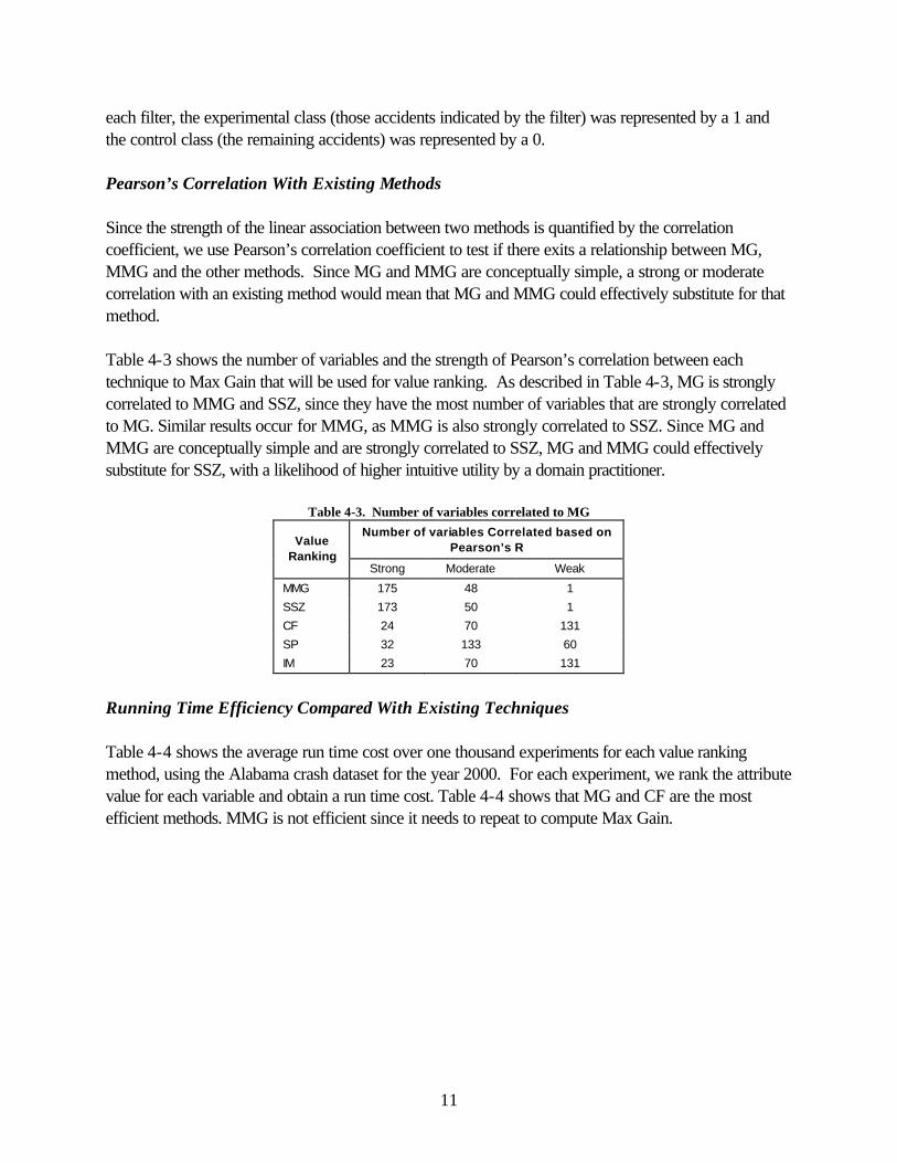
each filter, the experimental class (those accidents indicated by the filter) was represented by a 1 and the control class (the remaining accidents) was represented by a 0. Pearson’s Correlation With Existing Methods Since the strength of the linear association between two methods is quantified by the correlation coefficient, we use Pearson’s correlation coefficient to test if there exits a relationship between MG, MMG and the other methods. Since MG and MMG are conceptually simple, a strong or moderate correlation with an existing method would mean that MG and MMG could effectively substitute for that method. Table 4-3 shows the number of variables and the strength of Pearson’s correlation between each technique to Max Gain that will be used for value ranking. As described in Table 4-3, MG is strongly correlated to MMG and SSZ, since they have the most number of variables that are strongly correlated to MG. Similar results occur for MMG, as MMG is also strongly correlated to SSZ. Since MG and MMG are conceptually simple and are strongly correlated to SSZ, MG and MMG could effectively substitute for SSZ, with a likelihood of higher intuitive utility by a domain practitioner.
Table 4-3. Number of variables correlated to MG Number of variables Correlated based on
Pearson’s R Value Ranking
Strong Moderate Weak
MMG 175 48 1
SSZ 173 50 1
CF 24 70 131
SP 32 133 60
IM 23 70 131
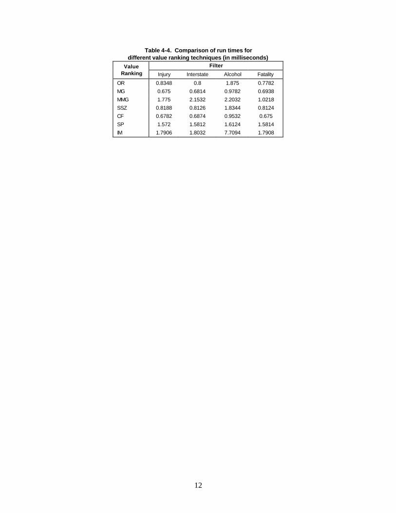
Running Time Efficiency Compared With Existing Techniques Table 4-4 shows the average run time cost over one thousand experiments for each value ranking method, using the Alabama crash dataset for the year 2000. For each experiment, we rank the attribute value for each variable and obtain a run time cost. Table 4-4 shows that MG and CF are the most efficient methods. MMG is not efficient since it needs to repeat to compute Max Gain.
12
Table 4-4. Comparison of run times for different value ranking techniques (in milliseconds)
Filter Value Ranking Injury Interstate Alcohol Fatality
OR 0.8348 0.8 1.875 0.7782
MG 0.675 0.6814 0.9782 0.6938
MMG 1.775 2.1532 2.2032 1.0218
SSZ 0.8188 0.8126 1.8344 0.8124
CF 0.6782 0.6874 0.9532 0.675
SP 1.572 1.5812 1.6124 1.5814
IM 1.7906 1.8032 7.7094 1.7908
13
Section 5 Variable Ranking
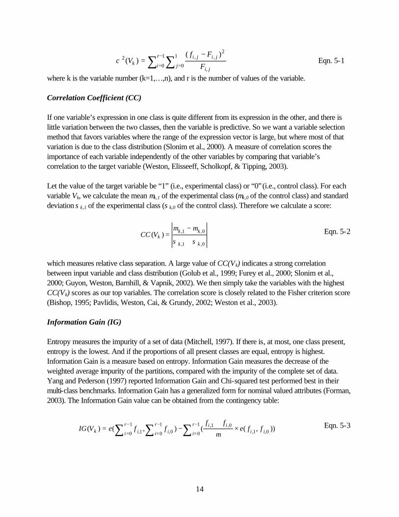
The Variable Ranking Problem The problem of variable ranking can be described in the notation provided by Guyon and Elisseeff (2003). We consider a training dataset with m records {xt; yt} (t = 1,…,m), each record consists of n input variables xt,k (k = 1,…,n) and one target variable yt. The input variables are noted as Vk (k = 1,…,n). Then we get a score S(Vk) of each variable Vi according to a particular variable ranking method computed from the corresponding contingency table. We assume that a higher score of a variable indicates a valuable variable and that the input variables are independent of each other. The variables are then sorted in decreasing order of S(Vk) allowing us to select the top most x variables of interest. We can construct the contingency table for each variable Vk (k = 1, …, n) as described in section 3. Various variable ranking methods have been proposed. In the following, we present the ranking methods we applied. Existing variable ranking methods The following sections describe existing variable ranking methods including Chi-squared (CHI) (Lehmann, 1959; Hawley, 1996; Leonrd, 2000), Correlation Coefficient (CC) (Golub et al., 1999; Furey et al., 2000; Slonim et al., 2000; Guyon, Weston, Barnhill, & Vapnik, 2002), Information Gain (IG) (Mitchell, 1997, Yang & Pedersen, 1997) and Gain Ratio (GR) (Grimaldi, Cunningham, & Kokaram, 2003). The limitation of these methods will be discussed in section 6. Chi-squared (CHI) The Chi-squared test (Lehmann, 1959; Hawley, 1996; Leonard, 2000) is one of the most widely used statistical tests. It can be used to test if there is ‘no association’ between two categorical variables. ‘No association’ means that for an individual, the response for one variable is not affected in any way by the response for another variable. This implies the two variables are independent. The Chi-squared measure can be used to find the variables that have significant Over-Representation (association) in regard to the target variable. The Chi-squared test can be calculated from a contingency table (Yang & Pedersen, 1997; Forman, 2003). The Chi-squared value can be obtained by the equation below:
14
∑ ∑−
= =
−=
1
0
1
0,
2,,2 )(
)(r
i jji
jijik F
FfVχ
where k is the variable number (k=1,…,n), and r is the number of values of the variable. Correlation Coefficient (CC) If one variable’s expression in one class is quite different from its expression in the other, and there is little variation between the two classes, then the variable is predictive. So we want a variable selection method that favors variables where the range of the expression vector is large, but where most of that variation is due to the class distribution (Slonim et al., 2000). A measure of correlation scores the importance of each variable independently of the other variables by comparing that variable’s correlation to the target variable (Weston, Elisseeff, Scholkopf, & Tipping, 2003). Let the value of the target variable be “1” (i.e., experimental class) or “0” (i.e., control class). For each variable Vk, we calculate the mean µk,1 of the experimental class (µk,0 of the control class) and standard deviation σk,1 of the experimental class (σk,0 of the control class). Therefore we calculate a score:
0,1,
0,1,)(kk
kkkVCC
σσ
µµ
+
−=
which measures relative class separation. A large value of CC(Vk) indicates a strong correlation between input variable and class distribution (Golub et al., 1999; Furey et al., 2000; Slonim et al., 2000; Guyon, Weston, Barnhill, & Vapnik, 2002). We then simply take the variables with the highest CC(Vk) scores as our top variables. The correlation score is closely related to the Fisher criterion score (Bishop, 1995; Pavlidis, Weston, Cai, & Grundy, 2002; Weston et al., 2003). Information Gain (IG) Entropy measures the impurity of a set of data (Mitchell, 1997). If there is, at most, one class present, entropy is the lowest. And if the proportions of all present classes are equal, entropy is highest. Information Gain is a measure based on entropy. Information Gain measures the decrease of the weighted average impurity of the partitions, compared with the impurity of the complete set of data. Yang and Pederson (1997) reported Information Gain and Chi-squared test performed best in their multi-class benchmarks. Information Gain has a generalized form for nominal valued attributes (Forman, 2003). The Information Gain value can be obtained from the contingency table:
∑∑∑ −
=
−
=
−
=×
+−=
1
0 0,1,0,1,1
0 0,1
0 1, )),((),()(r
i iiiir
i ir
i ik ffem
ffffeVIG
Eqn. 5-1
Eqn. 5-2
Eqn. 5-3
15
where yxy
yxy
yxx
yxx
yxe++
−++
−= 22 loglog),(, k is the variable number (k=1,…,n), r is the number of
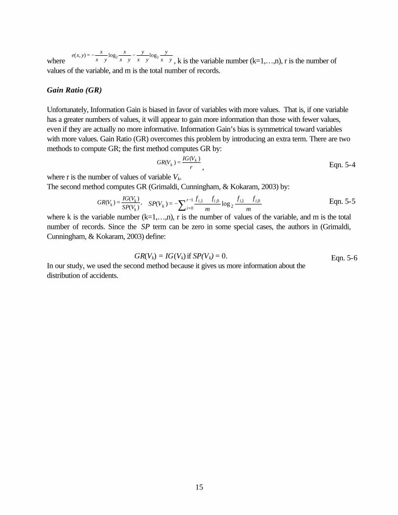
values of the variable, and m is the total number of records. Gain Ratio (GR) Unfortunately, Information Gain is biased in favor of variables with more values. That is, if one variable has a greater numbers of values, it will appear to gain more information than those with fewer values, even if they are actually no more informative. Information Gain’s bias is symmetrical toward variables with more values. Gain Ratio (GR) overcomes this problem by introducing an extra term. There are two methods to compute GR; the first method computes GR by:
rVIG
VGR kk
)()( =
, where r is the number of values of variable Vk. The second method computes GR (Grimaldi, Cunningham, & Kokaram, 2003) by:
,)()(
)(k
kk VSP
VIGVGR =
m
ff
m
ffVSP iir
i
iik
0,1,1
0 20,1, log)(
++−= ∑ −
= where k is the variable number (k=1,…,n), r is the number of values of the variable, and m is the total number of records. Since the SP term can be zero in some special cases, the authors in (Grimaldi, Cunningham, & Kokaram, 2003) define:
GR(Vk) = IG(Vk) if SP(Vk) = 0. In our study, we used the second method because it gives us more information about the distribution of accidents.
Eqn. 5-4
Eqn. 5-6
Eqn. 5-5
16
Section 6 A New Variable Ranking Method
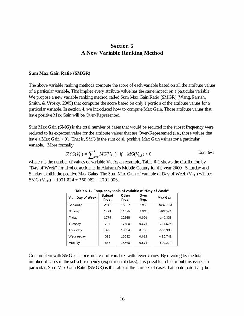
Sum Max Gain Ratio (SMGR) The above variable ranking methods compute the score of each variable based on all the attribute values of a particular variable. This implies every attribute value has the same impact on a particular variable. We propose a new variable ranking method called Sum Max Gain Ratio (SMGR) (Wang, Parrish, Smith, & Vrbsky, 2005) that computes the score based on only a portion of the attribute values for a particular variable. In section 4, we introduced how to compute Max Gain. Those attribute values that have positive Max Gain will be Over-Represented. Sum Max Gain (SMG) is the total number of cases that would be reduced if the subset frequency were reduced to its expected value for the attribute values that are Over-Represented (i.e., those values that have a Max Gain > 0). That is, SMG is the sum of all positive Max Gain values for a particular variable. More formally:
0)()()( ,1
0 , >= ∑ −
= ikr
i ikk VMGifVMGVSMG
where r is the number of values of variable Vk. As an example, Table 6-1 shows the distribution by “Day of Week” for alcohol accidents in Alabama’s Mobile County for the year 2000. Saturday and Sunday exhibit the positive Max Gains. The Sum Max Gain of variable of Day of Week (V008) will be: SMG (V008) = 1031.824 + 760.082 = 1791.906.
Table 6-1. Frequency table of variable of “Day of Week”
V008: Day of Week Subset Freq.
Other Freq.
Over Rep.
Max Gain
Saturday 2012 15837 2.053 1031.824
Sunday 1474 11535 2.065 760.082
Friday 1275 22868 0.901 -140.335
Tuesday 737 17750 0.671 -361.574
Thursday 872 19954 0.706 -362.983
Wednesday 693 18092 0.619 -426.741
Monday 667 18860 0.571 -500.274
One problem with SMG is its bias in favor of variables with fewer values. By dividing by the total number of cases in the subset frequency (experimental class), it is possible to factor out this issue. In particular, Sum Max Gain Ratio (SMGR) is the ratio of the number of cases that could potentially be
Eqn. 6-1

17
reduced by an effective countermeasure (SMG) to the total number of cases associated with the Over-Represented values (i.e., those cases where the Max Gain > 0). That is:
∑ −
=>=
1
0 ,1, 0)(/)()(r
i ikikk VMGiffVSMGVSMGR
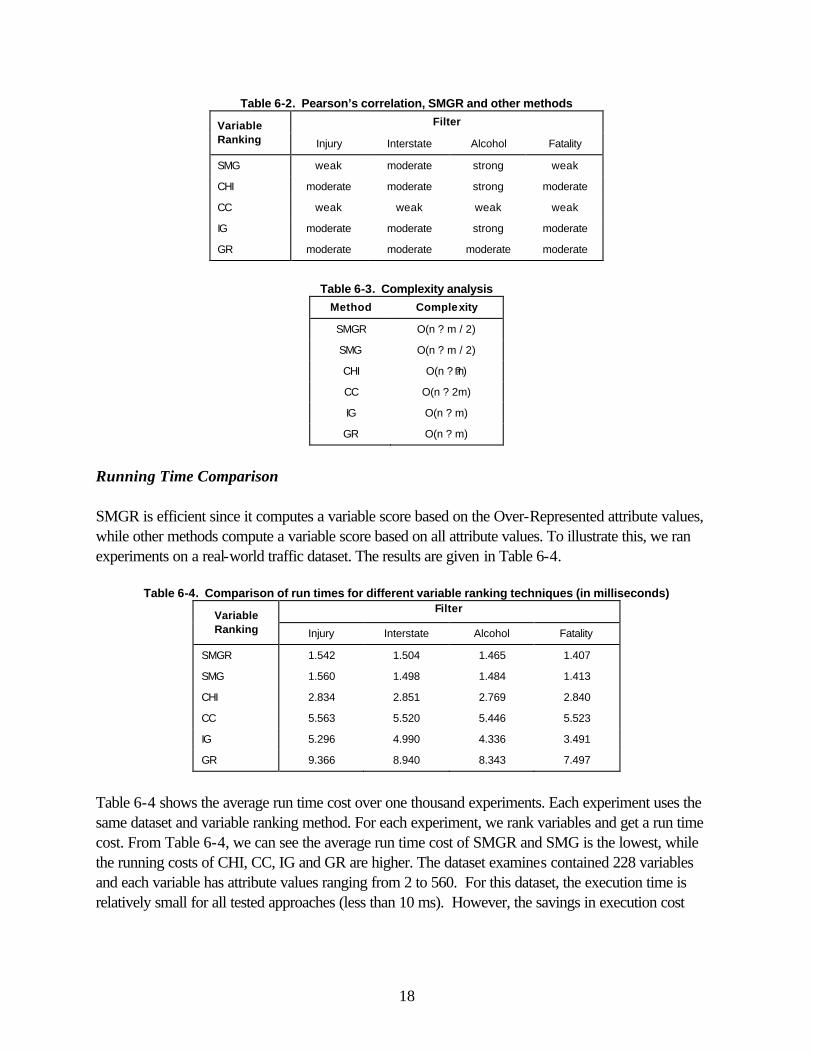
where r is the number of values of variable Vk. The SMG of variable “Day of Week” was computed from the above example to be 1791.906 (1031.824 + 760.082). Saturday and Sunday have positive Max Gain, and these two attribute values are Over-Represented. The total number of cases associated with the Over-Represented values will be 3486 (the sum of 2012 and 1474). The SMGR will be 0.514 (1791.906 / 3486 = 0.514). SMGR is always in the range of 0 to 1 because SMG is always less than the corresponding subset frequency. A high score of SMGR is indicative of a valuable variable with a high degree of relevance to the filter subset (experimental group). When presented in decreasing SMGR order, the most relevant variables are at the top. Results Using SMGR To compare the performance of SMGR to the other ranking methods, we used the Alabama Mobile County accident dataset for the year 2000. The target variables were selected by applying the filters of Injury, Interstate, Alcohol, and Fatality, respectively. The following sections compare the Pearson’s correlation between SMGR and existing variable ranking methods, the run time performance, predictive ability. Pearson’s Correlation With Existing Methods Since the strength of the linear association between two methods is quantified by the correlation coefficient, we use Pearson’s correlation coefficient to test if there exits a relationship between Sum Max Gain Ratio and any other method. Since SMGR is conceptually simple, a strong correlation with an existing method would mean that SMGR could effectively substitute for that method. Table 6-2 shows the Pearson’s correlation coefficient between SMGR and the other variable ranking methods. SMGR is correlated to CHI, IG and GR. Table 6-3 shows the complexity of each method. For complexity comparison, n is the number of variables and m is the number of attribute values. SMGR may be preferable to other variable ranking methods because of its conceptual simplicity and less complexity.
Eqn. 6-2
18
Table 6-2. Pearson’s correlation, SMGR and other methods Filter Variable
Ranking Injury Interstate Alcohol Fatality
SMG weak moderate strong weak
CHI moderate moderate strong moderate
CC weak weak weak weak
IG moderate moderate strong moderate
GR moderate moderate moderate moderate
Table 6-3. Complexity analysis
Method Complexity
SMGR O(n ? m / 2)
SMG O(n ? m / 2)
CHI O(n ? ?m)
CC O(n ? 2m)
IG O(n ? m)
GR O(n ? m)
Running Time Comparison SMGR is efficient since it computes a variable score based on the Over-Represented attribute values, while other methods compute a variable score based on all attribute values. To illustrate this, we ran experiments on a real-world traffic dataset. The results are given in Table 6-4.
Table 6-4. Comparison of run times for different variable ranking techniques (in milliseconds) Filter
Variable Ranking Injury Interstate Alcohol Fatality
SMGR 1.542 1.504 1.465 1.407
SMG 1.560 1.498 1.484 1.413
CHI 2.834 2.851 2.769 2.840
CC 5.563 5.520 5.446 5.523
IG 5.296 4.990 4.336 3.491
GR 9.366 8.940 8.343 7.497
Table 6-4 shows the average run time cost over one thousand experiments. Each experiment uses the same dataset and variable ranking method. For each experiment, we rank variables and get a run time cost. From Table 6-4, we can see the average run time cost of SMGR and SMG is the lowest, while the running costs of CHI, CC, IG and GR are higher. The dataset examines contained 228 variables and each variable has attribute values ranging from 2 to 560. For this dataset, the execution time is relatively small for all tested approaches (less than 10 ms). However, the savings in execution cost

19
(50%) of SMGR to the second closest approach will have significant implications for large datasets with tens or hundreds of thousands of variables, and when the attribute value of a variable is diverse. Classification In order to evaluate how our method of variable ranking affected classification, we employed the well known classification algorithm C4.5 (Quinlan, 1993) on the traffic accident data. We used C4.5 as an induction algorithm to evaluate the error rate on selected variables for each variable ranking method. C4.5 is an algorithm for inducing classification rules in the form of a decision tree from a given dataset. Nodes in a decision tree correspond to features and the leaves of the tree correspond to classes. The branches in a decision tree correspond to their association rule. C4.5 was applied to the datasets filtered through the different variable ranking methods. We used the Injury filter as described above to define the target variable. The top 25 best variables were selected through different variable ranking methods. Table 6-5 shows the error rate and the size of the decision tree for each variable ranking method.
Table 6-5. Results for the C4.5 algorithm
Method Error rate Size of the tree
(# of nodes)
SMGR 0.7% 32
SMG 1.0% 81
CHI 0.9% 159
CC 7.2% 13070
IG 0.9% 159
GR 0.7% 32
As seen in the experimental results, SMGR, CHI, IG and GR did not significantly change the generalization performance and these methods performed much better than CC. Table 6-5 also shows how variable ranking methods affects the size of the trees (the number of nodes in a tree) induced by C4.5. Smaller trees allow a better understanding of the decision tree. The size of the resulting tree generated by SMGR and GR showed a decrease from the maximum of 14438 nodes to 32 nodes, accompanied by a slight improvement in accuracy. To summarize, SMG and SMGR perform better than CHI, CC and IG.
20
Section 7 Using column-major storage to improve variable selection performance
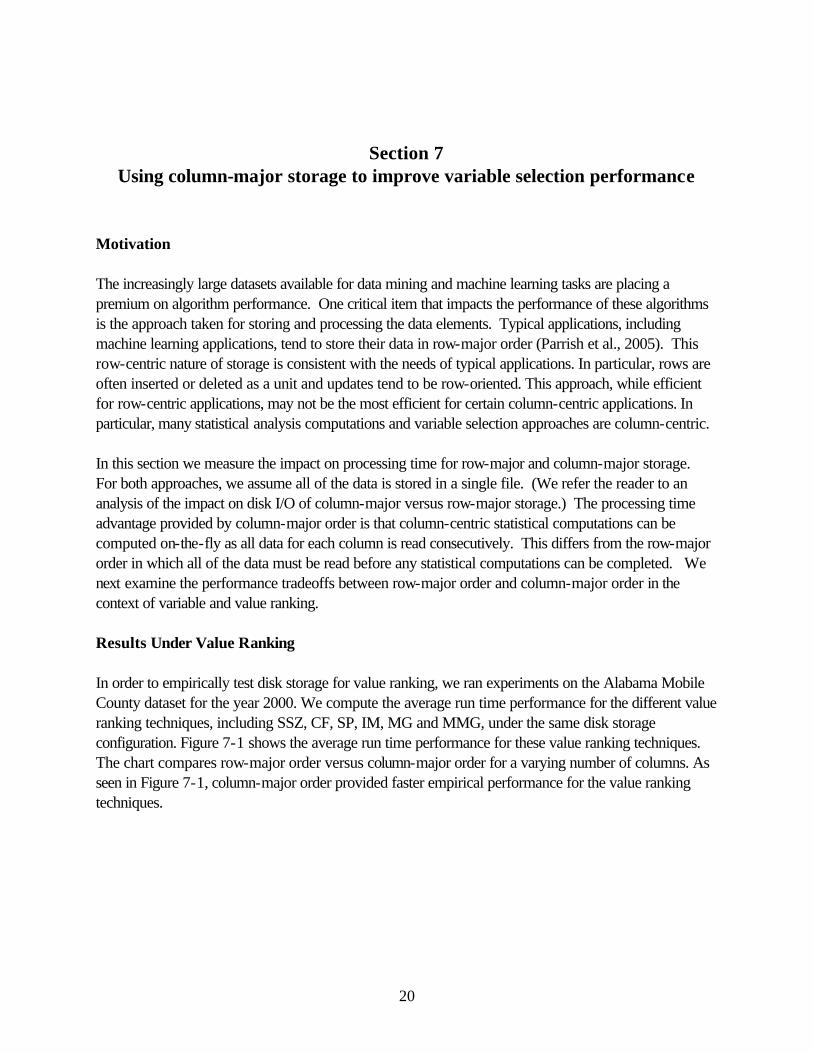
Motivation The increasingly large datasets available for data mining and machine learning tasks are placing a premium on algorithm performance. One critical item that impacts the performance of these algorithms is the approach taken for storing and processing the data elements. Typical applications, including machine learning applications, tend to store their data in row-major order (Parrish et al., 2005). This row-centric nature of storage is consistent with the needs of typical applications. In particular, rows are often inserted or deleted as a unit and updates tend to be row-oriented. This approach, while efficient for row-centric applications, may not be the most efficient for certain column-centric applications. In particular, many statistical analysis computations and variable selection approaches are column-centric. In this section we measure the impact on processing time for row-major and column-major storage. For both approaches, we assume all of the data is stored in a single file. (We refer the reader to an analysis of the impact on disk I/O of column-major versus row-major storage.) The processing time advantage provided by column-major order is that column-centric statistical computations can be computed on-the-fly as all data for each column is read consecutively. This differs from the row-major order in which all of the data must be read before any statistical computations can be completed. We next examine the performance tradeoffs between row-major order and column-major order in the context of variable and value ranking. Results Under Value Ranking In order to empirically test disk storage for value ranking, we ran experiments on the Alabama Mobile County dataset for the year 2000. We compute the average run time performance for the different value ranking techniques, including SSZ, CF, SP, IM, MG and MMG, under the same disk storage configuration. Figure 7-1 shows the average run time performance for these value ranking techniques. The chart compares row-major order versus column-major order for a varying number of columns. As seen in Figure 7-1, column-major order provided faster empirical performance for the value ranking techniques.
21
Figure 7-1. Average value ranking performance, column-major versus row-major
Results under variable ranking To compare the performance of row-major order and column-major order in the context of variable ranking, we used the Alabama Mobile County accident dataset for the year 2000. The dataset contains 14,218 records (i.e., rows) and 228 variables (i.e., columns). The target variable was selected by applying the filter of Injury. The experimental class (those accidents indicated by the filter) was represented by a “1” and the control class (the remaining accidents) was represented by a “0.” To facilitate generating datasets with varying numbers of rows and columns, and to assist in creating row-major and column-major storage options, the original dataset from the CARE application was transferred to Microsoft Excel for manipulation. The manipulated datasets were stored from Microsoft Excel as ASCII files. The variable selection algorithms were developed in C++ and manipulated the datasets in the ASCII files.
0
10
20
30
40
50
60
70
80
90
100
217
1085
2170
3255
4340
5425
6510
7595
8680
9765
1085
0
Number of columns
Ave
rage
run
tim
e pe
rfor
man
ce f
or d
iffer
ent
valu
e ra
nkin
g te
chni
ques
(in
sec
onds
)
row-major
column-major
22
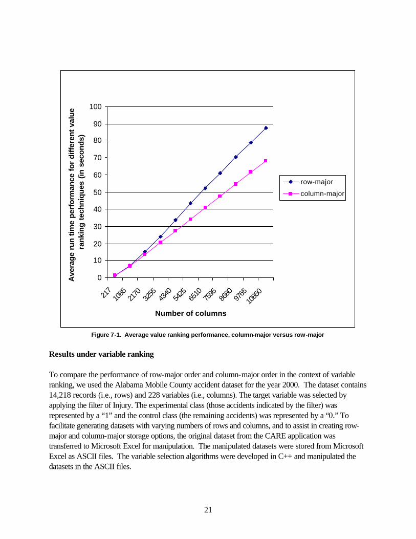
For each particular variable selection approach on each different dataset, we run one experiment and get a run time cost. One thousand of the same experiments were run to obtain an average run time cost. Figure 7-2 and Figure 7-3 illustrate the performance differences between the row-major order and column-major order storage methods in the context of SMGR by utilizing specific values for the dataset size, number of rows, number of columns, etc. The figures show the average run time cost in seconds, for a varying number of data values accessed.
Figure 7-2. Performance comparison, row-major versus column-major, fixed number of rows, SMGR.
Figure 7-2 illustrates the number of seconds to perform the variable selection of SMGR for a varying number of columns but a constant number of rows. The figure illustrates the results for 14,218 records (i.e., rows). The diagonal lines illustrate the run time cost for variable selection using the row-major and column-major methods. The run time ranges from 1.415 to 86.3 seconds using row-major order, while the run time ranges from 1.356 to 66.1 seconds using column-major order. As illustrated in Figure 3,
0
10
20
30
40
50
60
70
80
90
100
217 1085
2170
3255
4340
5425
6510
7595
8680
9765
1085
0
Number of columns
Ave
rag
e ru
n t
ime
per
form
ance
fo
r S
MG
R (
in s
eco
nd
s)
row-major
column-major

23
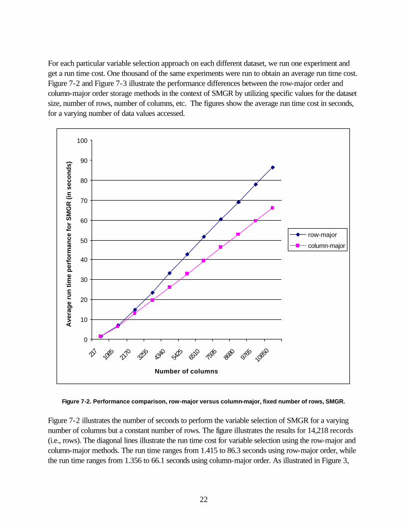
after approximately one thousand columns, the run time cost of row-major order processing increases faster than the column order processing. In this experiment, column order processing outperforms row order regardless of the selection algorithm used. Figure 7-3 illustrates the number of seconds to perform variable selection with a varying number of rows but a constant of columns.
Figure 7-3. Performance comparison, row-major versus column-major, fixed columns, SMGR
Figure 7-3 illustrates the result for 217 columns (i.e., variables). The plot illustrates the run time cost to do variable selection using both row-major and column-major methods. As illustrated in the figure, the run time cost is almost the same using row order and column order until up to approximately 14,000 rows in the dataset. From that point, the run time cost for the row order increases slightly faster than using the column order.
0
10
20
30
40
50
60
70
80
1421
871
090
1421
80
2132
70
2843
60
3554
50
4265
40
4976
30
5687
20
6398
10
7109
00
Number of rows
Ave
rag
e ru
n ti
me
oer
form
ance
for
SM
GR
(in
sec
on
d)
row-major
column-major
24
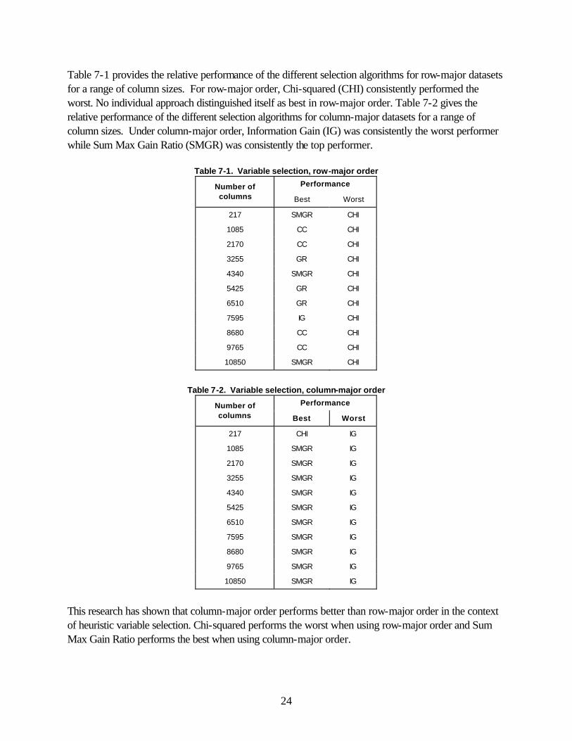
Table 7-1 provides the relative performance of the different selection algorithms for row-major datasets for a range of column sizes. For row-major order, Chi-squared (CHI) consistently performed the worst. No individual approach distinguished itself as best in row-major order. Table 7-2 gives the relative performance of the different selection algorithms for column-major datasets for a range of column sizes. Under column-major order, Information Gain (IG) was consistently the worst performer while Sum Max Gain Ratio (SMGR) was consistently the top performer.
Table 7-1. Variable selection, row-major order Performance Number of
columns Best Worst
217 SMGR CHI
1085 CC CHI
2170 CC CHI
3255 GR CHI
4340 SMGR CHI
5425 GR CHI
6510 GR CHI
7595 IG CHI
8680 CC CHI
9765 CC CHI
10850 SMGR CHI
Table 7-2. Variable selection, column-major order
Performance Number of columns Best Worst
217 CHI IG
1085 SMGR IG
2170 SMGR IG
3255 SMGR IG
4340 SMGR IG
5425 SMGR IG
6510 SMGR IG
7595 SMGR IG
8680 SMGR IG
9765 SMGR IG
10850 SMGR IG
This research has shown that column-major order performs better than row-major order in the context of heuristic variable selection. Chi-squared performs the worst when using row-major order and Sum Max Gain Ratio performs the best when using column-major order.
25
Section 8 Integration with CARE
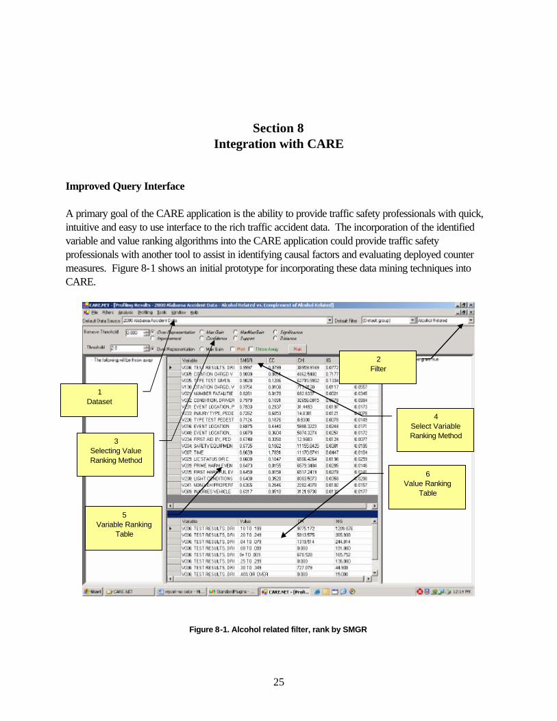
Improved Query Interface A primary goal of the CARE application is the ability to provide traffic safety professionals with quick, intuitive and easy to use interface to the rich traffic accident data. The incorporation of the identified variable and value ranking algorithms into the CARE application could provide traffic safety professionals with another tool to assist in identifying causal factors and evaluating deployed counter measures. Figure 8-1 shows an initial prototype for incorporating these data mining techniques into CARE.
Figure 8-1. Alcohol related filter, rank by SMGR
5 Variable Ranking
Table
3 Selecting Value Ranking Method
4 Select Variable Ranking Method
6 Value Ranking
Table
2 Filter
1 Dataset
26
Figure 8-1 shows the ranking of variables using the alcohol filter for the year 2000 Alabama Accident Dataset. Table 8-1 describes the highlighted boxes in the diagram:
Table 8-1. Description of featured elements in Figure 8-1
Box Description
1 The dataset selected
2 The filter selected
3 The value ranking method to be used
4 The variable ranking method to be used for sorting the table
5 The variable ranking table sorted by the appropriate method
6 Values for the selected variable sorted by the appropriate value ranking method
Table 8-2 summarizes the top five variables selected by SMGR as shown in Figure 8-1.
Table 8-2. Summary of top five variables from Figure 8-1
Rankin
g Variabl
e Label Description
1 V0036 Test Results Driver C Indicates the results for the Blood Alcohol Test given.
2 V0065 Citation Charged, Vehicle C Indicates that a citation was
given to the causal driver
3 V0035 Type Test Given Driver C Indicates the type of test given
the causal driver
4 V0130 Citation Charged, Vehicle 2 Indicates that a citation was
given a second vehicle
5 V0021 Number Fatalities Indicates the number of fatalities in the accident
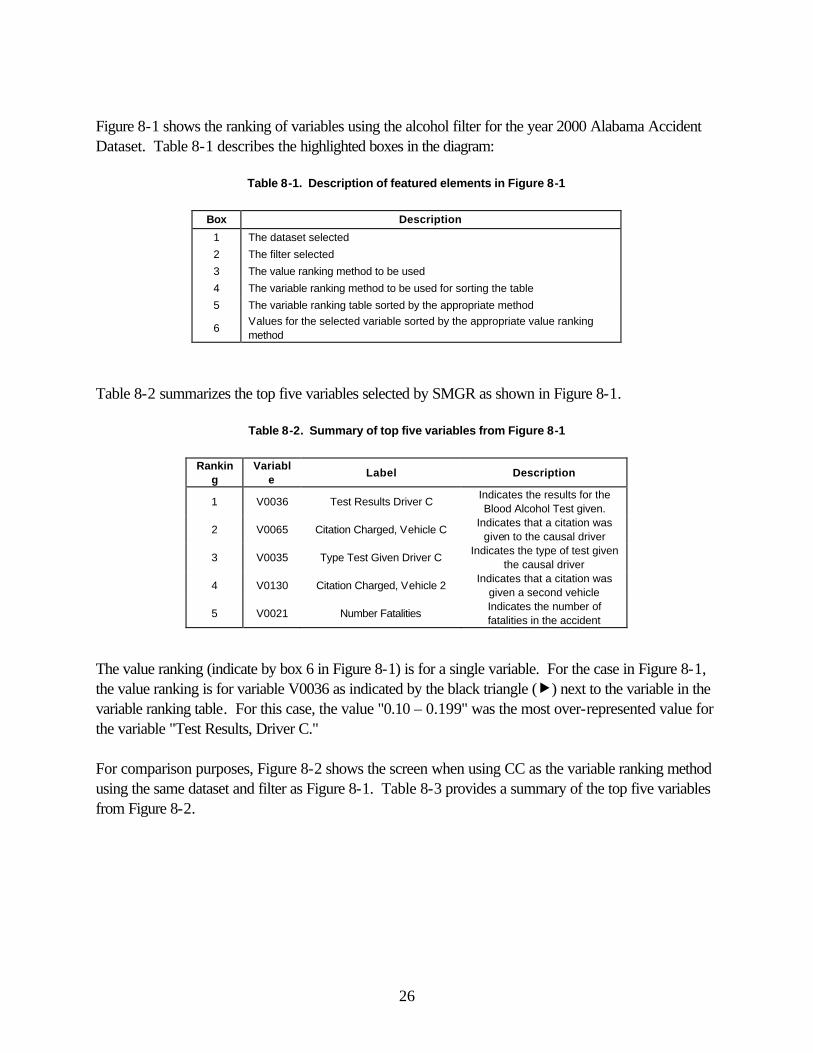
The value ranking (indicate by box 6 in Figure 8-1) is for a single variable. For the case in Figure 8-1, the value ranking is for variable V0036 as indicated by the black triangle (�) next to the variable in the variable ranking table. For this case, the value "0.10 – 0.199" was the most over-represented value for the variable "Test Results, Driver C." For comparison purposes, Figure 8-2 shows the screen when using CC as the variable ranking method using the same dataset and filter as Figure 8-1. Table 8-3 provides a summary of the top five variables from Figure 8-2.
27
Figure 8-2. Alcohol related filter, rank by CC
Table 8-3. Summary of top five variables from Figure 8-2
Ranking
Variable
Label Description
1 V0003 Month The month the accident occurred
2 V0006 Week The week of the accident beginning with January 1 – January 7 as Week 1
3 V0004 Date of Month The date of the month the accident occurred ( between 1 and 31)
4 V0126 Dir of travel Vehicle 2
Indicates the direction of travel for a second vehicle involved in the accident. (North, South, East, West, Unknown)
5 V0008 Day of Week The day of the week of the accident.
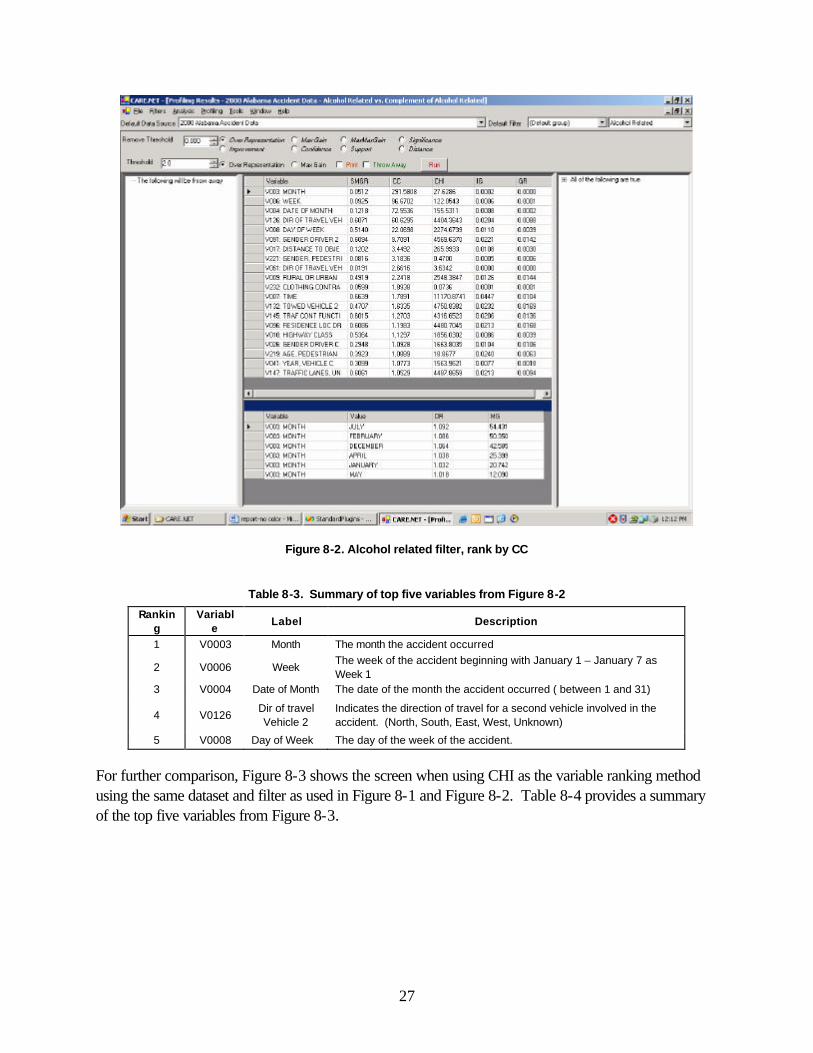
For further comparison, Figure 8-3 shows the screen when using CHI as the variable ranking method using the same dataset and filter as used in Figure 8-1 and Figure 8-2. Table 8-4 provides a summary of the top five variables from Figure 8-3.
28
Figure 8-3. Alcohol related filter, rank by CHI
Table 8-4. Summary of top five variables from Figure 8-3
Ranking
Variable
Label Description
1 V0035 Test Results
Driver C Indicates the results for the Blood Alcohol Test given.
2 V0036 Citation Charged,
Vehicle C Indicates that a citation was given to the causal driver
3 V0032 Condition, Driver C Indicates the officer's assessment of the causal drivers condition to include apparently asleep, ill, fatigued, etc.
4 V0007 Time Time of day of the accident
5 V0034 Safety Equipment,
Driver C
Indicates the officer’s assessment of the type of safety equipment available and used by the causal driver. This includes lap and shoulder belts and air bags.
29
Section 9 Conclusions
In this research, we have presented a value ranking method called Max Gain (MG). MG is a very intuitive method, in that it serves as a metric that has definitive meaning to a practitioner, particularly within the traffic safety domain discussed here. In particular, MG gives the maximum potential for reduction in crashes, given the application of a countermeasure designed to reduce crashes. Thus, MG allows the practitioner to make resource tradeoffs among countermeasures, based on real numbers. MG is not only useful as a metric, but is also useful as a value ranking method. In particular, MG is strongly correlated with SSZ and outperforms most of the previous value ranking techniques, making it a conceptually simpler proxy for SSZ. It is also moderately correlated with SP, making it a potential proxy for SP as well. We also present a variable ranking method called Sum Max Gain Ratio (SMGR). SMGR is derived from MG and uses Over-Represented attribute values as the primary contributing factor in variable ranking. The experiments have shown SMGR performs well at variable ranking with less run time cost than more traditional approaches, such as Chi-squared and Information Gain. In certain cases, it was empirically shown to provide a faster run time with similar variable rankings. The findings suggest that SMGR is more sensitive to the number of variables (columns) than to the number of records (rows). In addition, we examined the performance tradeoffs between row-major order and column-major order in the context of heuristic variable selection. The research has shown that column-major order performs better than row-major order in the context of heuristic variable selection and value ranking.
30
Section 10 References
Agrawal, R., Imielinski, T., & Swami, A. (1993). Mining association rules between sets of items in large databases. Proceedings of ACM SIGMOD Conference on Management of Data, Washington DC, 207-216.
Andrews, H. C. (1971). Multidimensional rotations in feature selection. TC, 20(9), 1045. Baim, P. W. (1988). A method for attribute selection in inductive learning systems. IEEE Transactions
on Pattern Analysis and Machine Intelligence, 10(6), 888-896. Berry, M., & Linoff, G. (1997). Data mining techniques: For marketing, sales, and customer
support. John Wiley & Sons, Inc. Bishop, C. (1995). Neural networks for pattern recognition. Oxford University Press, Oxford. Caruana, R., & Freitag, D. (1994). Greedy attribute selection. Proceedings of 11th International
Conference on Machine Learning, 28-36. Forman, G. (2003). An extensive empirical study of feature selection metrics for text classification.
Journal of Machine Learning Research, 3(Mar):1289-1305. Foster, D. P., & Stine, R. A. (2004). Variable selection in data mining: building a predictive model for
bankruptcy. Journal of the American Statistical Association, 99(466), 303-313. Fukunaga, K., & Koontz, W. L. G. (1970). Application of karhunen-loeve expansion to feature
selection and ordering. TC, 19(4), 311. Furey, T., Cristianini, N., Duffy, N., & Bednarski, D. W., Schummer, M., & Haussler, D. (2000).
Support vector machine classification and validation of cancer tissue samples using microarray expression data. Bioinformatics, 16(10), 906-914.
Golub, T. R., et al. (1999). Molecular classification of cancer: Class discovery and class prediction by gene expression monitoring. Science, 286(5439), 531-537.
Grimaldi, M., Cunningham, P., & Kokaram, A. (2003). An evaluation of alternative feature selection strategies and ensemble techniques for classifying music. The 14th European Conference on Machine Learning and the 7th European Conference on Principles and Practice of Knowledge Discovery in Databases, Dubrovnik, Croatia.
Guyon, I., Weston, J., Barnhill, S. & Vapnik, V. (2002). Gene selection for cancer classification using support vector machines. Machine Learning, 46(1-3), 389–422.
Guyon, I., & Elisseeff, A. (2003). An introduction to variable and feature selection. Journal of Machine Learning Research, 3(Mar), 1157-1182.
Hall, M. A., & Smith, L. A. (1999). Feature selection for machine learning: comparing a correlation-based filter approach to the wrapper. Proceedings of the Florida Artificial Intelligence Symposium, Orlando, Florida, 235-239.
Hall, M. A., & Holmes, G. (2003). Benchmarking attribute selection techniques for discrete class data mining. IEEE Transactions on Knowledge and Data Engineering, 15(6), 1437-1447.
Hawley. W. (1996). Foundations of statistics. Harcourt Brace & Company. Howell, D. C. (2001). Statistical methods for psychology (5th ed.). Duxbury: Belmont, CA.
31
Kautardzic, M (2001). Data mining – concepts, models, methods and algorithms. IEEE Press. Kohavi, R., John, G., & Pfleger, K. (1994). Irrelevant features and the subset selection problem.
Proceedings of 11th International Conference on Machine Learning, New Brunswick, NJ, 121-129.
Kohavi, R., & John, G. (1997). Wrappers for feature subset selection. Artificial Intelligence, 97(1-2), 273-324.
Lehmann, E. L. (1959). Testing statistical hypothesis. Wiley, New York. Leonard, T. (2000). A course in categorical data analysis. Chpman & Hall CRC. Mitchell, T. M. (1997). Machine learning. McGraw-Hill. Mladenic, D., & Grobelnik, M. (1999). Feature selection for unbalanced class distribution and naïve
bayes. Proceedings of the 16th International Conference on Machine Learning, 258-267. Pappa, G. L., Freitas, A. A., & Kaestner, C. A. A. (2002). A multiobjective genetic algorithm for
attribute selection. Proceedings of 4th International Conference on Recent Advances in Soft Computing (RASC), 116-121.
Parrish, A., Dixon, B., Cordes, D., Vrbsky, S., & Brown, D. (2003). CARE: A tool to analyze automobile crash data. IEEE Computer 36(6), 22-30.
Parrish, A., Vrbsky, S., Dixon, B., & Ni, W. (2005). Optimizing disk storage to support statistical analysis operations. Decision Support Systems Journal, 38(4), 621-628.
Pavlidis, P., Weston, J., Cai, J., & Grundy, W. N. (2002). Learning gene functional classifications from multiple data types. Journal of Computational Biology, 9(2), 401-411.
Quinlan, J. R. (1993). C4.5: programs for machine learning. Los Altos, California: Morgan Kaufmann.
Richards, W. D. (2002). The Zen of empirical research (quantitative methods) in communication. Hampton press, Inc.
Slonim, D., Tamayo, P., Mesirov, J., Golub, T., & Lander, E. (2000). Class prediction and discovery using gene expression data. Proceedings of 4th Annual International Conference on Computational Molecular Biology Universal Academy Press, Tokyo, Japan, 263-272.
Srikant, R., & Agrawal, R. (1995). Mining generalized association rules. Proceedings of 21th VLDB Conference, Zurich, Swizerland.
Stockburger, D. W. (1996). Introductory statistics: Concepts, Models, and Applications. Stoppiglia, H., Dreyfus, G., Dubois, R., & Oussar, Y. (2003). Ranking a random feature for variable
and feature selection. Journal of Machine Learning Research, 3(Mar), 1399-1414. Viallefont, V., Raftery, A. E., & Richardson, S. (2001). Variable selection and Bayesian model
averaging in epidemiological case-control studies. Statistics in Medicine, 20, 3215-3230. Wang, H., Parrish, A., & Chen, H. C. (2003). Automated selection of automobile crash
countermeasures. Proceedings of 41th ACM Southeast Regional Conference, 268-273. Wang, H., Parrish, A., Smith, R., & Vrbsky, S. (2005). Variable selection and ranking for analyzing
automobile traffic accident data. Proceedings of the 20th ACM Symposium on Applied Computing, Santa Fe, New Mexico, 36-41.
Weston, J., Elisseff, A., Scholkopf, B., & Tipping, M. (2003). Use of the zero-norm with linear models and kernel methods. Journal of Machine Learning Research, 3(Mar), 1439-1461.

32
Yang, Y., & Pedersen, J. O. (1997). A comparative study on feature selection in text categorization. Proceedings of the 14th International Conference on Machine Learning, 412-420.
Zembowicz. R., & Zytkow, J. (1996). From contingency tables to various forms of knowledge in databases. Advances in Knowledge Discovery and Data Mining, AAAI Press/The MIT Press, 328-349.