Embed Size (px)
Citation preview

Data Mining
2007
Ian H. Witten
Data Mining Algorithms
Ian H. Witten
Computer Science DepartmentWaikato University
New Zealand
http://www.cs.waikato.ac.nz/~ihwhttp://www.cs.waikato.ac.nz/ml/weka
The problem
Classification (“supervised”)Given A set of classified examplesProduce A way of classifying new examples
Instances: described by fixed set of featuresClasses: discrete or continuous
Interested in:Results? (classifying new instances)Model? (how the decision is made)
“instances”
“attributes”“classification” “regression”
Association rulesLook for rules that relate features to other features
Clustering (“unsupervised”)There are no classes
Simplicity first!
Simple algorithms often work very well!
There are many kinds of simple structure, eg: One attribute does all the work All attributes contribute equally and independently A decision tree involving tests on a few attributes Rules that assign instances to classes Distance in instance space from a few class “prototypes” Result depends on a linear combination of attributes
Success of method depends on the domain
Agenda
A very simple strategy Overfitting, evaluation
Statistical modeling Bayes rule
Constructing decision trees Constructing rules
+ Association rules
Linear models Regression, perceptrons, neural nets, SVMs, model trees
Instance-based learning and clustering Hierarchical, probabilistic clustering
Engineering the input and output Attribute selection, data transformations, PCA Bagging, boosting, stacking, co-training
One attribute does all the work
Learn a 1-level decision tree i.e., rules that all test one particular attribute
Basic version One branch for each value Each branch assigns most frequent class Error rate: proportion of instances that don’t belong to
the majority class of their corresponding branch Choose attribute with smallest error rate
For each attribute,For each value of the attribute, make a rule as follows:
count how often each class appearsfind the most frequent classmake the rule assign that class to this attribute-value
Calculate the error rate of this attribute’s rulesChoose the attribute with the smallest error rate
Example
3/6True → No*
5/142/8False → YesWind
1/7Normal → Yes
4/143/7High → NoHumidity
5/14
4/14
Totalerrors
1/4Cool → Yes
2/6Mild → Yes
2/4Hot → No*Temp
2/5Rainy → Yes
0/4Overcast → Yes
2/5Sunny → NoOutlook
ErrorsRulesAttribute
* indicates a tie
NoTrueHighMildRainy
YesFalseNormalHotOvercast
YesTrueHighMildOvercast
YesTrueNormalMildSunny
YesFalseNormalMildRainy
YesFalseNormalCoolSunny
NoFalseHighMildSunny
YesTrueNormalCoolOvercast
NoTrueNormalCoolRainy
YesFalseNormalCoolRainy
YesFalseHighMildRainy
YesFalseHighHotOvercast
NoTrueHighHotSunny
NoFalseHighHotSunny
PlayWindHumidityTempOutlook

Data Mining
2007
Ian H. Witten
Complications: Missing values
Omit instances where the attribute value is missing Treat “missing” as a separate possible value
“Missing” means what? Unknown? Unrecorded? Irrelevant?
Is there significance in the fact that a value is missing?
Nominal vs numeric values for attributes
Complications: Overfitting
……………
YesFalse8075Rainy
YesFalse8683Overcast
NoTrue9080Sunny
NoFalse8585Sunny
PlayWindHumidityTempOutlook
0/14
Totalerrors
……
0/175 → No
0/183 → Yes
0/080 → Yes
0/185 → NoTemp
ErrorsRulesAttribute
Memorization vs generalization Do not evaluate rules on the training data Here, independent test data shows poor performance To fix, use
Training data — to form rules Validation data — to decide on best rule Test data — to determine system performance
Evaluate on training set? — NO!
Independent test set
Cross-validation
Stratified cross-validation
Stratified 10-fold cross-validation,repeated 10 times
Leave-one-out
The “Bootstrap”
Evaluating the result
This incredibly simple methodwas described in a 1993 paper An experimental evaluation on 16 datasets Used cross-validation so that results were
representative of performance on new data Simple rules often outperformed far more
complex methods
Simplicity first pays off!
“Very Simple Classification Rules Perform Well on MostCommonly Used Datasets”Robert C. Holte, Computer Science Department, University of Ottawa
One attribute does all the work
Agenda
A very simple strategy Overfitting, evaluation
Statistical modeling Bayes rule
Constructing decision trees Constructing rules
+ Association rules
Linear models Regression, perceptrons, neural nets, SVMs, model trees
Instance-based learning and clustering Hierarchical, probabilistic clustering
Engineering the input and output Attribute selection, data transformations, PCA Bagging, boosting, stacking, co-training
Statistical modeling
Opposite strategy: use all the attributes Two assumptions: Attributes are
equally important a priori statistically independent (given the class value)
I.e., knowing the value of one attribute says nothingabout the value of another (if the class is known)
Independence assumption is never correct! But … often works well in practice
One attribute does all the work?

Data Mining
2007
Ian H. Witten
Probability of event H given evidence E
A priori probability of H Probability of event before evidence is seen
A posteriori probability of H Probability of event after evidence is seen
Bayes’s rule
]Pr[
]Pr[]|Pr[]|Pr[
E
HHEEH =
]|Pr[ EH
]Pr[H
Thomas BayesBritish mathematician and Presbyterian ministerBorn 1702 Died 1761
!
Pr[H | E] =Pr[E
1|H]Pr[E
1|H]...Pr[E
n|H]Pr[H]
Pr[E]
“Naïve” assumption: Evidence splits into parts that are independent
instanceclass
Weather data: probabilities
5/14
5
No
9/14
9
Yes
Play
3/5
2/5
3
2
No
3/9
6/9
3
6
Yes
True
False
True
False
Wind
1/5
4/5
1
4
NoYesNoYesNoYes
6/9
3/9
6
3
Normal
High
Normal
High
Humidity
1/5
2/5
2/5
1
2
2
3/9
4/9
2/9
3
4
2
Cool2/53/9Rainy
Mild
Hot
Cool
Mild
Hot
Temperature
0/54/9Overcast
3/52/9Sunny
23Rainy
04Overcast
32Sunny
Outlook
NoTrueHighMildRainy
YesFalseNormalHotOvercast
YesTrueHighMildOvercast
YesTrueNormalMildSunny
YesFalseNormalMildRainy
YesFalseNormalCoolSunny
NoFalseHighMildSunny
YesTrueNormalCoolOvercast
NoTrueNormalCoolRainy
YesFalseNormalCoolRainy
YesFalseHighMildRainy
YesFalseHighHotOvercast
NoTrueHighHotSunny
NoFalseHighHotSunny
PlayWindHumidityTempOutlook
5/14
5
No
9/14
9
Yes
Play
3/5
2/5
3
2
No
3/9
6/9
3
6
Yes
True
False
True
False
Wind
1/5
4/5
1
4
NoYesNoYesNoYes
6/9
3/9
6
3
Normal
High
Normal
High
Humidity
1/5
2/5
2/5
1
2
2
3/9
4/9
2/9
3
4
2
Cool2/53/9Rainy
Mild
Hot
Cool
Mild
Hot
Temperature
0/54/9Overcast
3/52/9Sunny
23Rainy
04Overcast
32Sunny
Outlook
?TrueHighCoolSunny
PlayWindHumidityTemp.Outlook A new day:
Likelihood of the two classes
For “yes” = 2/9 × 3/9 × 3/9 × 3/9 × 9/14 = 0.0053
For “no” = 3/5 × 1/5 × 4/5 × 3/5 × 5/14 = 0.0206
Conversion into a probability by normalization:
P(“yes”) = 0.0053 / (0.0053 + 0.0206) = 0.205
P(“no”) = 0.0206 / (0.0053 + 0.0206) = 0.795
Weather data: probabilities
?TrueHighCoolSunny
PlayWindHumidityTemp.Outlook Evidence E
Probability ofclass “yes”
]|Pr[]|Pr[ yesSunnyOutlookEyes ==
]|Pr[ yesCooleTemperatur =!
]|Pr[ yesHighHumidity =!
]|Pr[ yesTrueWindy =!
]Pr[
]Pr[
E
yes!
]Pr[
149
93
93
93
92
E
!!!!=
Weather data: probabilities
Training: do not include instance in frequencycount for attribute value-class combination
Classification: omit attribute from calculation Example:
Missing values
?TrueHighCool?
PlayWindHumidityTemp.Outlook
Likelihood of “yes” = 3/9 × 3/9 × 3/9 × 9/14 = 0.0238
Likelihood of “no” = 1/5 × 4/5 × 3/5 × 5/14 = 0.0343
P(“yes”) = 0.0238 / (0.0238 + 0.0343) = 41%
P(“no”) = 0.0343 / (0.0238 + 0.0343) = 59%
ComplicationsZero frequencies
An attribute value doesn’t occur with every class Probability will be zero! 0]|Pr[ == yesHighHumidity
Numeric attributes
Often assume attributes have a Gaussian distribution(given the class)
Its probability density function is definedby two parameters:
Sample mean
Standard deviation
The density function is
!=
=n
i
ix
n 1
1µ
!=
""
=n
i
ix
n 1
2)(1
1µ#
2
2
2
)(
2
1)( !
µ
!"
##
=
x
exf
Carl Friedrich GaussGerman mathematician and scientist“The prince of mathematicians”Born 1777 Died 1855

Data Mining
2007
Ian H. Witten
Numeric attributes
Often assume attributes have a Gaussian distribution(given the class)
Its probability density function is definedby two parameters:
Sample mean
Standard deviation
The density function is
!=
=n
i
ix
n 1
1µ
!=
""
=n
i
ix
n 1
2)(1
1µ#
2
2
2
)(
2
1)( !
µ
!"
##
=
x
exf
A new day:?true9066Sunny
PlayWindHumidityTemp.Outlook
Likelihood of “yes” = 2/9 × 0.0340 × 0.0221 × 3/9 × 9/14 = 0.000036
Likelihood of “no” = 3/5 × 0.0291 × 0.0380 × 3/5 × 5/14 = 0.000136
P(“yes”) = 0.000036 / (0.000036 + 0. 000136) = 20.9%
P(“no”) = 0.000136 / (0.000036 + 0. 000136) = 79.1%
“Naïve” statistical model
Naïve = assume attributes are independent
Naïve Bayes works surprisingly well even if independence assumption is clearly violated
Why? Because classification doesn’t require accurate
probability estimates so long as the greatest probability is assigned to the
correct class
But: adding redundant attributes causes problems e.g. identical attributes
And: numeric attributes may not be normallydistributed → kernel density estimators
Agenda
A very simple strategy Overfitting, evaluation
Statistical modeling Bayes rule
Constructing decision trees Constructing rules
+ Association rules
Linear models Regression, perceptrons, neural nets, SVMs, model trees
Instance-based learning and clustering Hierarchical, probabilistic clustering
Engineering the input and output Attribute selection, data transformations, PCA Bagging, boosting, stacking, co-training
Constructing decision trees
Strategy: top downRecursive divide-and-conquer fashion First: select attribute for root node
Create branch for each possibleattribute value
Then: split instances into subsetsOne for each branch extendingfrom the node
Finally: repeat recursively for each branch,using only instances that reach the branch
Stop if all instances have the same class
Which attribute to select? Which is the best attribute?
Criterion: want to get the smallest tree Heuristic
choose the attribute that produces the “purest” nodes I.e. the greatest information gain
Information theory: measure information in bits
Information gain Amount of information gained by knowing the value of
the attribute Entropy of distribution before the split
– entropy of distribution after it
!
entropy(p1, p2,..., pn ) = "p1logp1 " p2logp2..." pnlogpn
Claude ShannonAmerican mathematician and scientist“The father of information theory”Born 1916 Died 2001

Data Mining
2007
Ian H. Witten
Which attribute to select?
0.247 bits0.152 bits
0.048 bits 0.029 bits
Continuing to split
gain(temperature ) = 0.571 bitsgain(humidity ) = 0.971 bitsgain(windy ) = 0.020 bits
Complications
Highly-branching attributes Extreme case: ID code
n
m
l
k
j
i
h
g
f
e
d
c
b
a
ID code
NoTrueHighMildRainy
YesFalseNormalHotOvercast
YesTrueHighMildOvercast
YesTrueNormalMildSunny
YesFalseNormalMildRainy
YesFalseNormalCoolSunny
NoFalseHighMildSunny
YesTrueNormalCoolOvercast
NoTrueNormalCoolRainy
YesFalseNormalCoolRainy
YesFalseHighMildRainy
YesFalseHighHotOvercast
NoTrueHighHotSunny
NoFalseHighHotSunny
PlayWindHumidityTempOutlook
Info gain is maximal(0.940 bits)
Complications
Highly-branching attributes Extreme case: ID code
Overfitting: need to prune
goodgoodgoodbad{good,bad}Acceptability of contracthalffull?none{none,half,full}Health plan contributionyes??no{yes,no}Bereavement assistancefullfull?none{none,half,full}Dental plan contributionyes??no{yes,no}Long-term disability assistanceavggengenavg{below-avg,avg,gen}Vacation12121511(Number of days)Statutory holidays???yes{yes,no}Education allowance
Shift-work supplementStandby payPensionWorking hours per weekCost of living adjustmentWage increase third yearWage increase second yearWage increase first yearDuration
Attribute
44%5%?Percentage??13%?Percentage???none{none,ret-allw, empl-cntr}40383528(Number of hours)none?tcfnone{none,tcf,tc}????Percentage4.04.4%5%?Percentage4.54.3%4%2%Percentage2321(Number of years)
40…321Type
Complications
Highly-branching attributes Extreme case: ID code
Overfitting: need to prune
Complications
Highly-branching attributes Extreme case: ID code
Overfitting: need to prune Prepruning vs postpruning
Missing values During training During testing: “fractional instances”
Numeric attributes Choose best “split point” for attribute E.g. temp < 25

Data Mining
2007
Ian H. Witten
The most extensively studied method of machinelearning used in data mining
Different criteria for attribute selection rarely make a large difference
Different pruning methods mainly change the size of the pruned tree
Univariate vs multivariate decision trees Single vs compound tests at the nodes
C4.5 and CART
Constructing decision treesTop-down induction of decision trees
Ross QuinlanAustralian computer scientistUniversity of Sydney
Agenda
A very simple strategy Overfitting, evaluation
Statistical modeling Bayes rule
Constructing decision trees Constructing rules
+ Association rules
Linear models Regression, perceptrons, neural nets, SVMs, model trees
Instance-based learning and clustering Hierarchical, probabilistic clustering
Engineering the input and output Attribute selection, data transformations, PCA Bagging, boosting, stacking, co-training
Constructing rules
Convert (top-down) decision tree into a rule set Straightforward, but rule set overly complex More effective conversions are not trivial
Alternative: (bottom-up) covering method for each class in turn find rule set that covers all
instances in it(excluding instances not in the class)
Separate-and-conquer method First identify a useful rule Then separate out all the instances it covers Finally “conquer” the remaining instances
Cf divide-and-conquer methods: No need to explore subset covered by rule any further
Generating a rule
y
x
a
b b
b
b
b
bb
b
b bb
b
bb
aa
aa
a
y
a
b b
b
b
b
bb
b
b bb
b
bb
aa
aa
a
x1·2
y
a
b b
b
b
b
bb
b
b bb
b
bb
aa
aa
a
x1·2
2·6
If x > 1.2then class = a
If x > 1.2 and y > 2.6then class = a
If truethen class = a
Possible rule set for class “b”:
Could add more rules, get “perfect” rule set
If x ≤ 1.2 then class = bIf x > 1.2 and y ≤ 2.6 then class = b
Corresponding decision tree:(produces exactly the samepredictions)
Rule sets can be more perspicuous E.g. when decision trees contain replicated subtrees
Also: in multiclass situations, covering algorithm concentrates on one class at a time decision tree learner takes all classes into account
Rules vs. trees
If x ≤ 1.2 then class = bIf x > 1.2 and y ≤ 2.6 then class = b
For each class C Initialize E to the instance set While E contains instances in class C
Create a rule R that predicts class C(with empty left-hand side)
Until R is perfect(or there are no more attributes to use)
• For each attribute A not mentioned in R, and eachvalue v, Consider adding the condition A = v to the left-
hand side of R Select A and v to maximize the accuracy p/t
(break ties by choosing the condition with thelargest p)
• Add A = v to R
Remove the instances covered by R from E
Constructing rules

Data Mining
2007
Ian H. Witten
More about rules
Rules are order-dependent Two rules might assign different classes to an instance
Work through the classes in turn generating rules for that class
For each class a “decision list” is generated Subsequent rules are designed for instances that are
not covered by previous rules But: order doesn’t matter because all rules predict the
same class
Problems: overlapping rules For better rules: globalization optimization
Association rules
… can predict any attribute and combinations of attributes … are not intended to be used together as a set
Problem: immense number of possible associations Output needs to be restricted to show only the most
predictive associations
Define Support: number of instances predicted correctly Confidence: correct predictions as % of instances covered
Examples
Specify minimum support and confidence e.g. 58 rules with support ≥ 2 and confidence ≥ 95%
If temperature = cool then humidity = normal
NoTrueHighMildRainy
YesFalseNormalHotOvercast
YesTrueHighMildOvercast
YesTrueNormalMildSunny
YesFalseNormalMildRainy
YesFalseNormalCoolSunny
NoFalseHighMildSunny
YesTrueNormalCoolOvercast
NoTrueNormalCoolRainy
YesFalseNormalCoolRainy
YesFalseHighMildRainy
YesFalseHighHotOvercast
NoTrueHighHotSunny
NoFalseHighHotSunny
PlayWindHumidityTempOutlook
If Wind = false and play = nothen outlook = sunny and humidity = high
Support = 4, confidence = 100%
Support = 2, confidence = 100%
Constructing association rules
To find association rules: Use separate-and-conquer Treat every possible combination of attribute values as
a separate class
Two problems: Computational complexity Huge number of rules
(which would need pruning on the basis of support andconfidence)
But: we can look for high support rules directly! Generate frequent “item sets”
From them, generate and test possible rules
Temperature = Cool, Humidity = Normal, Wind = False, Play = Yes (2)
Temperature = Cool, Wind = False ⇒ Humidity = Normal, Play = YesTemperature = Cool, Wind = False, Humidity = Normal ⇒ Play = YesTemperature = Cool, Wind = False, Play = Yes ⇒ Humidity = Normal
(all have support 2, confidence = 100%)
Example association rules
Rules with support ≥ 2 and confidence 100%:
support=4 3 rules support=3 5 rules support=2 50 rules
total 58
100%2⇒ Humidity=HighOutlook=Sunny Temperature=Hot58
............
100%3⇒ Humidity=NormalTemperature=Cold Play=Yes4
100%4⇒ Play=YesOutlook=Overcast3
100%4⇒ Humidity=NormalTemperature=Cool2
100%4⇒ Play=YesHumidity=Normal Wind=False1
Association rule Conf.Sup.
Association rules: discussion
Market basket analysis: huge data sets
May not fit in main memory Different algorithms necessary Minimize passes through the data
Practical issue: generating a certain number of rules e.g. by incrementally reducing minimum support
Confidence is not necessarily the best measure e.g. milk occurs in almost every supermarket transaction Other measures have been devised (e.g. lift)
Buy beer ⇒ buy chipsDay = Thursday, buy beer ⇒ buy diapers
Agenda
A very simple strategy Overfitting, evaluation
Statistical modeling Bayes rule
Constructing decision trees Constructing rules
+ Association rules
Linear models Regression, perceptrons, neural nets, SVMs, model trees
Instance-based learning and clustering Hierarchical, probabilistic clustering
Engineering the input and output Attribute selection, data transformations, PCA Bagging, boosting, stacking, co-training
Data Mining
2007
Ian H. Witten
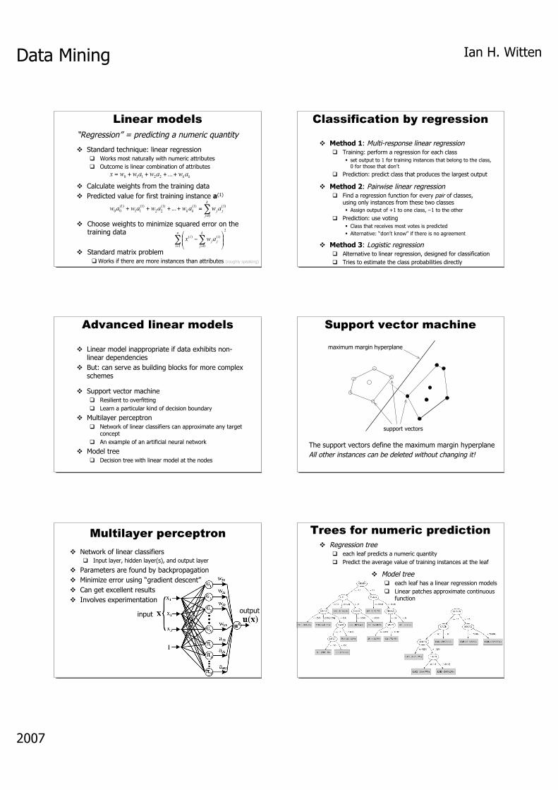
Linear models
Standard technique: linear regression Works most naturally with numeric attributes Outcome is linear combination of attributes
Calculate weights from the training data Predicted value for first training instance a(1)
kkawawawwx ++++= ...
22110
!=
=++++k
j
jjkk awawawawaw0
)1()1()1(
22
)1(
11
)1(
00 ...
Choose weights to minimize squared error on thetraining data
Standard matrix problem Works if there are more instances than attributes (roughly speaking)
2
1 0
)()(! != =
""#
$%%&
'(
n
i
k
j
i
jj
i awx
“Regression” = predicting a numeric quantity
Classification by regression
Method 1: Multi-response linear regression Training: perform a regression for each class
set output to 1 for training instances that belong to the class,0 for those that don’t
Prediction: predict class that produces the largest output
Method 2: Pairwise linear regression Find a regression function for every pair of classes,
using only instances from these two classes Assign output of +1 to one class, –1 to the other
Prediction: use voting Class that receives most votes is predicted Alternative: “don’t know” if there is no agreement
Method 3: Logistic regression Alternative to linear regression, designed for classification Tries to estimate the class probabilities directly
Advanced linear models
Linear model inappropriate if data exhibits non-linear dependencies
But: can serve as building blocks for more complexschemes
Support vector machine Resilient to overfitting Learn a particular kind of decision boundary
Multilayer perceptron Network of linear classifiers can approximate any target
concept An example of an artificial neural network
Model tree Decision tree with linear model at the nodes
Support vector machine
The support vectors define the maximum margin hyperplaneAll other instances can be deleted without changing it!
maximum margin hyperplane
support vectors
Multilayer perceptron
Network of linear classifiers Input layer, hidden layer(s), and output layer
Parameters are found by backpropagation Minimize error using “gradient descent” Can get excellent results Involves experimentation
input output
Trees for numeric prediction Regression tree
each leaf predicts a numeric quantity Predict the average value of training instances at the leaf
Model tree each leaf has a linear regression models Linear patches approximate continuous
function

Data Mining
2007
Ian H. Witten
Discussion of linear models
Linear regression: well-founded mathematicaltechnique
Can be used for classification in situations that are“linearly separable”
… but very susceptible to noise Support vector machines yield excellent performance
particularly in situations with many redundant attributes
Multilayer perceptrons (“neural nets”) can work well but often require much experimentation
Regression/model trees grew out of decision trees Regression trees were introduced in CART Model trees were developed by Quinlan
Agenda
A very simple strategy Overfitting, evaluation
Statistical modeling Bayes rule
Constructing decision trees Constructing rules
+ Association rules
Linear models Regression, perceptrons, neural nets, SVMs, model trees
Instance-based learning and clustering Hierarchical, probabilistic clustering
Engineering the input and output Attribute selection, data transformations, PCA Bagging, boosting, stacking, co-training
Instance-based learning
Search training set for instance that’s most like thenew one The instances themselves represent the “knowledge” Noise will be a problem
Similarity function defines what’s “learned” Euclidean distance Nominal attributes? Set to 1 if different, 0 if same Weight the attributes?
Lazy learning: do nothing until you have to Methods:
nearest-neighbor k-nearest-neighbor
“Rote learning” = simplest form of learning Often very accurate … but slow:
scan entire training data to make each prediction? sophisticated data structures can make this much faster
Assumes all attributes are equally important Remedy: attribute selection or weights
Remedies against noisy instances: Majority vote over the k nearest neighbors Weight instances according to their prediction accuracy Identify reliable “prototypes” for each class
Statisticians have used k-NN since 1950s If n → ∞ and k/n → 0, error approaches minimum
Instance-based learning
Clustering
No target value to predict Differences between models/algorithms:
Exclusive vs. overlapping Hierarchical vs. flat Incremental vs. batch learning Deterministic vs. probabilistic
Evaluation? Usually by inspection Clusters-to-classes evaluation? Probabilistic density estimation can be evaluated on
test data
Unsupervised vs supervised learning (classification)
Hierarchical clustering
Bottom up Start with single-instance clusters At each step, join the two closest clusters How to define the distance between clusters?
Distance between the two closest instances? Distance between the means
Top down Start with one universal cluster Find two clusters Proceed recursively
on each subset

Data Mining
2007
Ian H. Witten
To cluster data into k groups (k is predefined)
1. Choose k cluster centers (“seeds”) e.g. at random
2. Assign instances to clusters based on distance to cluster centroids
3. Compute centroids of clusters4. Go to step 1
until convergence
Results can depend strongly on initial seeds Can get trapped in local minumum
Rerun with different seeds?
Iterative: fixed num of clusters
The k-means algorithm
A 51A 43B 62B 64A 45A 42A 46A 45A 45
B 62A 47A 52B 64A 51B 65A 48A 49A 46
B 64A 51A 52B 62A 49A 48B 62A 43A 40
A 48B 64A 51B 63A 43B 65B 66B 65A 46
A 39B 62B 64A 52B 63B 64A 48B 64A 48
A 51A 48B 64A 42A 48A 41
Probabilistic clustering
Model data using a mixture of normal distributions One cluster, one distribution
governs probabilities of attribute values in that cluster
Finite mixtures : finite number of clusters
µA=50, σA =5, pA=0.6 µB=65, σB =2, pB=0.4
Learn the clusters ⇒ determine their parameter, ie mean, standard deviation
Performance criterion: likelihood of training data given the clusters
Iterative Expection-Maximization (EM) algorithm E step: Calculate cluster probability for each instance M step: Estimate distribution parameters from cluster probabilities
Finds a local maximum of the likelihood
Using the mixture model
Probability that instance x belongs to cluster A:
Likelihood of an instance given the clusters:
]Pr[
),;(
]Pr[
]Pr[]|Pr[]|Pr[
x
pxf
x
AAxxA AAA !µ
==2
2
2
)(
2
1),;( !
µ
!"!µ
#
=
x
exf
!=i
xx ]clusterPr[]cluster|Pr[]onsdistributi the|Pr[ ii
Extending the mixture model
More then two distributions: easy Several attributes: easy—assuming independence! Correlated attributes: difficult
Joint model: bivariate normal distribution with a(symmetric) covariance matrix
n attributes: need to estimate n + n (n+1)/2 parameters
Nominal attributes: easy (if independent) Missing values: easy Can use other distributions than normal:
“log-normal” if predetermined minimum is given “log-odds” if bounded from above and below Poisson for attributes that are integer counts
Unknown number of clusters: Use cross-validation to estimate k
Bayesian clustering
Problem: many parameters ⇒ EM overfits Bayesian approach : give every parameter a prior
probability distribution Incorporate prior into overall likelihood figure Penalizes introduction of parameters
Eg: Laplace estimator for nominal attributes Can also have prior on number of clusters! Implementation: NASA’s AUTOCLASS
Agenda
A very simple strategy Overfitting, evaluation
Statistical modeling Bayes rule
Constructing decision trees Constructing rules
+ Association rules
Linear models Regression, perceptrons, neural nets, SVMs, model trees
Instance-based learning and clustering Hierarchical, probabilistic clustering
Engineering the input and output Attribute selection, data transformations, PCA Bagging, boosting, stacking, co-training

Data Mining
2007
Ian H. Witten
Engineering the input & output
Attribute selection Scheme-independent, scheme-specific
Attribute discretization Unsupervised, supervised
Data transformations Ad hoc, Principal component analysis
Dirty data Data cleansing, robust regression, anomaly detection
Combining multiple models Bagging, randomization, boosting, stacking
Using unlabeled data Co-training
Just apply a learner? – NO!
Attribute selection
Adding a random (i.e. irrelevant) attribute cansignificantly degrade C4.5’s performance Problem: attribute selection based on smaller and
smaller amounts of data
IBL very susceptible to irrelevant attributes Number of training instances required increases
exponentially with number of irrelevant attributes
Naïve Bayes doesn’t have this problem Relevant attributes can also be harmful
Data transformations
Simple transformations can often make a largedifference in performance
Example transformations (not necessarily forperformance improvement): Difference of two date attributes Ratio of two numeric (ratio-scale) attributes Concatenating the values of nominal attributes Encoding cluster membership Adding noise to data Removing data randomly or selectively Obfuscating the data
Principal component analysis
Principal component analysis
Method for identifying the important “directions” inthe data
Can rotate data into (reduced) coordinate systemthat is given by those directions
Algorithm:1. Find direction (axis) of greatest variance2. Find direction of greatest variance that is perpendicular
to previous direction and repeat
Implementation: find eigenvectors of covariancematrix by diagonalization Eigenvectors (sorted by eigenvalues) are the directions
Combining multiple models
Basic idea:build different “experts,” let them vote
Advantage: often improves predictive performance
Disadvantage: usually produces output that is very hard to analyze but: there are approaches that aim to produce a single
comprehensible structure
Methods Bagging Randomization Boosting Stacking
Bagging
Combining predictions by voting/averaging Simplest way Each model receives equal weight
“Idealized” version: Sample several training sets of size n
(instead of just having one training set of size n) Build a classifier for each training set Combine the classifiers’ predictions
Learning scheme is unstable Þalmost always improves performance Small change in training data can make big change in
model (e.g. decision trees)

Data Mining
2007
Ian H. Witten
Randomization
Can randomize learning algorithm instead of input Some algorithms already have a random
component: eg. initial weights in neural net Most algorithms can be randomized, eg. greedy
algorithms: Pick from the N best options at random instead of
always picking the best options Eg.: attribute selection in decision trees
More generally applicable than bagging: e.g.random subsets in nearest-neighbor scheme
Can be combined with bagging
Boosting
Also uses voting/averaging Weights models according to performance Iterative: new models are influenced by
performance of previously built ones Encourage new model to become an “expert” for
instances misclassified by earlier models Intuitive justification: models should be experts that
complement each other
Several variants
Stacking
To combine predictions of base learners, don’t vote,use meta learner Base learners: level-0 models Meta learner: level-1 model Predictions of base learners are input to meta learner
Base learners are usually different schemes Can’t use predictions on training data to generate
data for level-1 model! Instead use cross-validation-like scheme
Hard to analyze theoretically: “black magic”
Using unlabeled data
Semisupervised learning: attempts to use unlabeleddata as well as labeled data The aim is to improve classification performance
Why try to do this? Unlabeled data is often plentifuland labeling data can be expensive Web mining: classifying web pages Text mining: identifying names in text Video mining: classifying people in the news
Leveraging the large pool of unlabeled exampleswould be very attractive
Co-training
Method for learning from multiple views (multiplesets of attributes), eg: First set of attributes describes content of web page Second set of attributes describes links that link to the
web page
Step 1: build model from each view Step 2: use models to assign labels to unlabeled
data Step 3: select those unlabeled examples that were
most confidently predicted (ideally, preserving ratioof classes)
Step 4: add those examples to the training set Step 5: go to Step 1 until data exhausted Assumption: views are independent
Agenda
A very simple strategy Overfitting, evaluation
Statistical modeling Bayes rule
Constructing decision trees Constructing rules
+ Association rules
Linear models Regression, perceptrons, neural nets, SVMs, model trees
Instance-based learning and Clustering Hierarchical, probabilistic clustering
Engineering the input and output Attribute selection, data transformations, PCA Bagging, boosting, stacking, co-training

Data Mining
2007
Ian H. Witten
Data mining algorithms
There is no magic in data mining Instead, a huge array of alternative techniques
There is no single universal “best method” Experiment! Which ones work best on your problem?
The WEKA machine learning workbench http://www.cs.waikato.ac.nz/ml/weka
Data mining: practical machine learning tools andtechniques by Ian H. Witten and Eibe Frank, 2005
Thank you for your attention!