Embed Size (px)
Citation preview

1
DATA MINING: NAÏVE BAYES
2
Naïve Bayes Classifier
We will start off with some mathematical background. But first we start with some visual intuition.
Thomas Bayes
1702 - 1761

3
An
ten
na
Le
ng
th
10
1 2 3 4 5 6 7 8 9 10
1
2
3
4
5
6
7
8
9
Grasshoppers Katydids
Abdomen Length
Remember this example? Let’s get lots more data…
4
An
ten
na
Le
ng
th
10
1 2 3 4 5 6 7 8 9 10
1
2
3
4
5
6
7
8
9
Katydids Grasshoppers
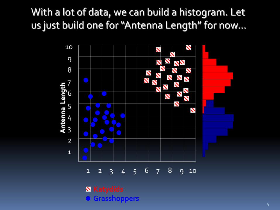
With a lot of data, we can build a histogram. Let us just build one for “Antenna Length” for now…
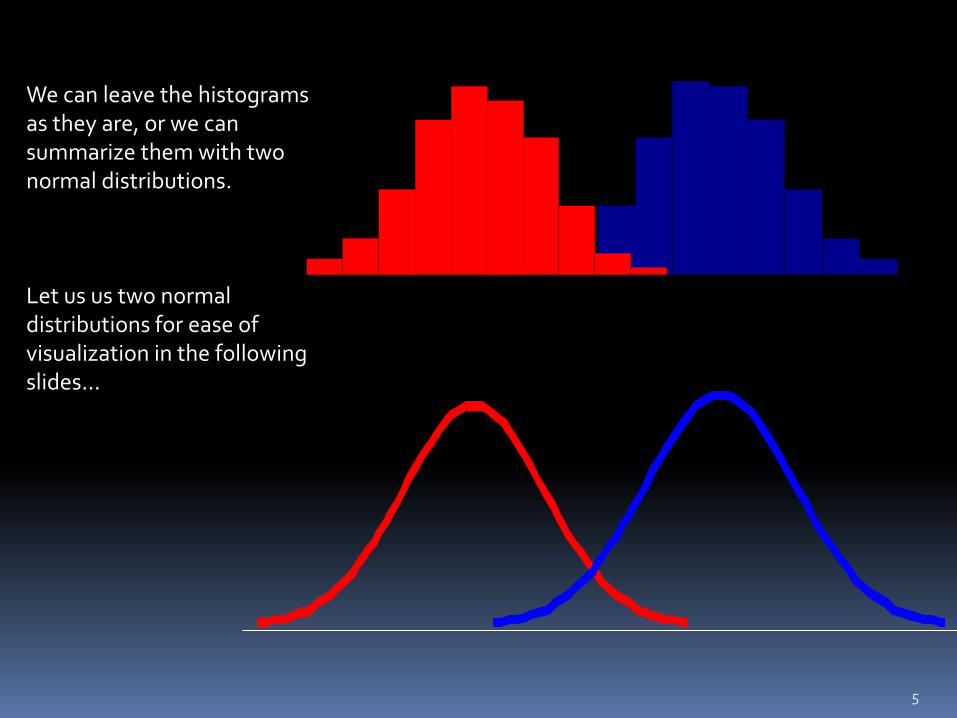
We can leave the histograms as they are, or we can summarize them with two normal distributions. Let us us two normal distributions for ease of visualization in the following slides…
5
3
Antennae length is 3
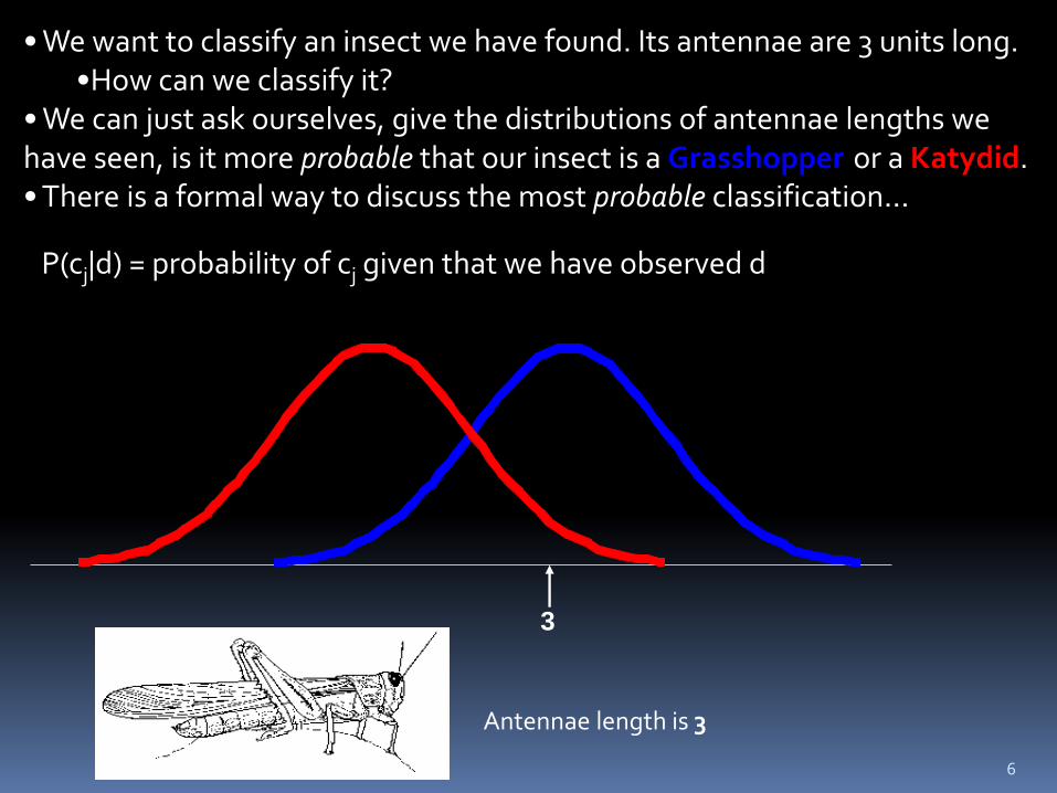
• We want to classify an insect we have found. Its antennae are 3 units long. •How can we classify it?
• We can just ask ourselves, give the distributions of antennae lengths we have seen, is it more probable that our insect is a Grasshopper or a Katydid. • There is a formal way to discuss the most probable classification…
6
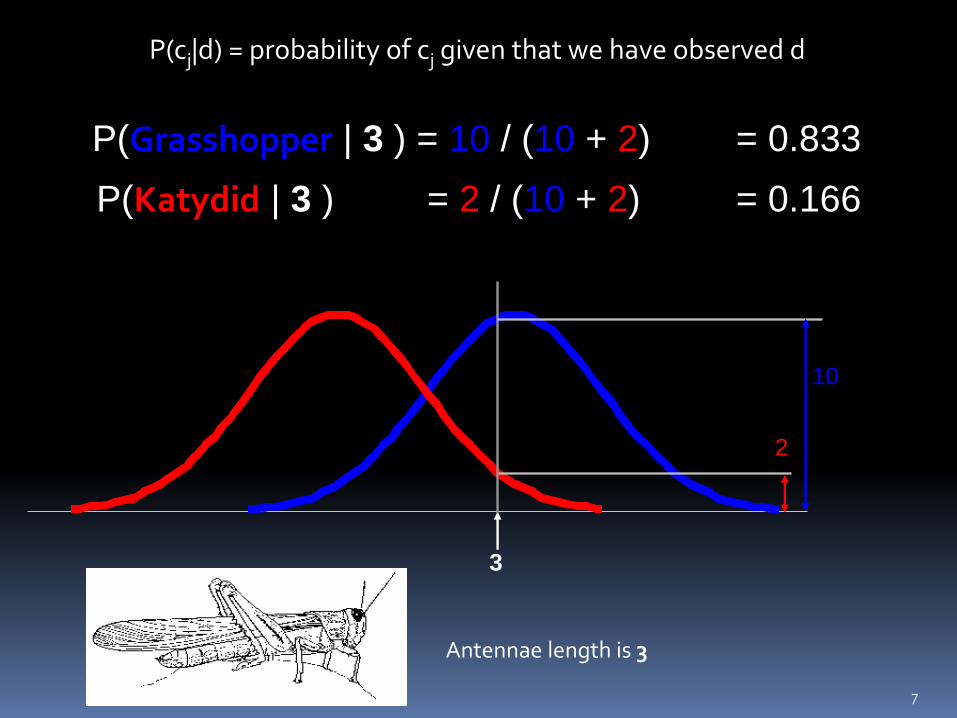
P(cj|d) = probability of cj given that we have observed d
10
2
P(Grasshopper | 3 ) = 10 / (10 + 2) = 0.833
P(Katydid | 3 ) = 2 / (10 + 2) = 0.166
3
Antennae length is 3
7
P(cj|d) = probability of cj given that we have observed d
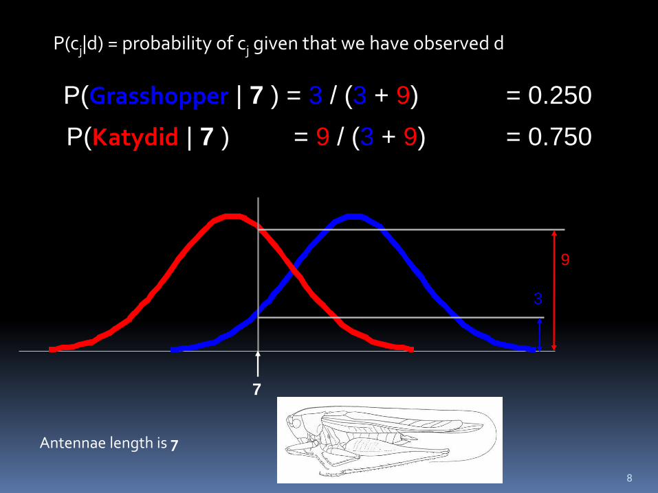
9
3
P(Grasshopper | 7 ) = 3 / (3 + 9) = 0.250
P(Katydid | 7 ) = 9 / (3 + 9) = 0.750
7
Antennae length is 7
8
P(cj|d) = probability of cj given that we have observed d
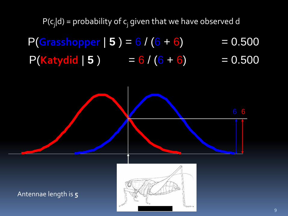
6 6
P(Grasshopper | 5 ) = 6 / (6 + 6) = 0.500
P(Katydid | 5 ) = 6 / (6 + 6) = 0.500
5
Antennae length is 5
9
P(cj|d) = probability of cj given that we have observed d
Bayes Classifier
A probabilistic framework for classification problems
Often appropriate because the world is noisy and also some relationships are probabilistic in nature
Is predicting who will win a baseball game probabilistic in nature?
Before getting the heart of the matter, we will go over some basic probability.
We will review the concept of reasoning with uncertainty, which is based on probability theory Should be review for many of you
10
Discrete Random Variables
A is a Boolean-valued random variable if A denotes an event, and there is some degree of uncertainty as to whether A occurs.
Examples A = The next patient you examine is suffering from inhalational
anthrax
A = The next patient you examine has a cough
A = There is an active terrorist cell in your city
We view P(A) as “the fraction of possible worlds in which A is true”
11
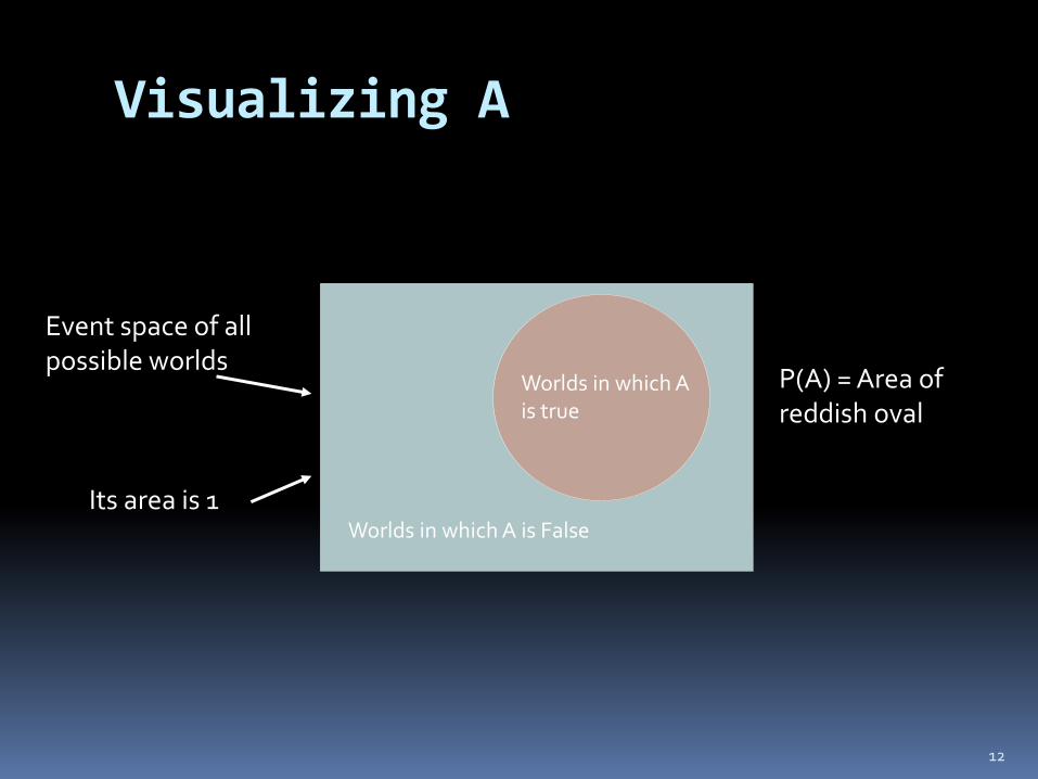
Visualizing A
12
Event space of all possible worlds
Its area is 1
Worlds in which A is False
Worlds in which A is true
P(A) = Area of reddish oval
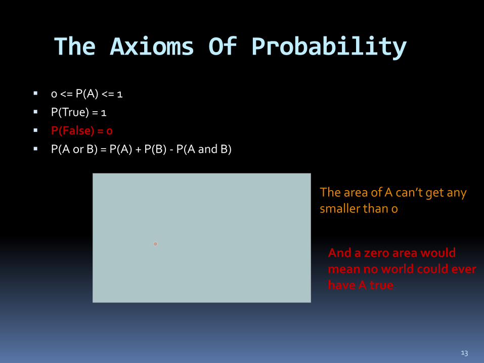
The Axioms Of Probability
0 <= P(A) <= 1
P(True) = 1
P(False) = 0
P(A or B) = P(A) + P(B) - P(A and B)
13
The area of A can’t get any smaller than 0
And a zero area would mean no world could ever have A true
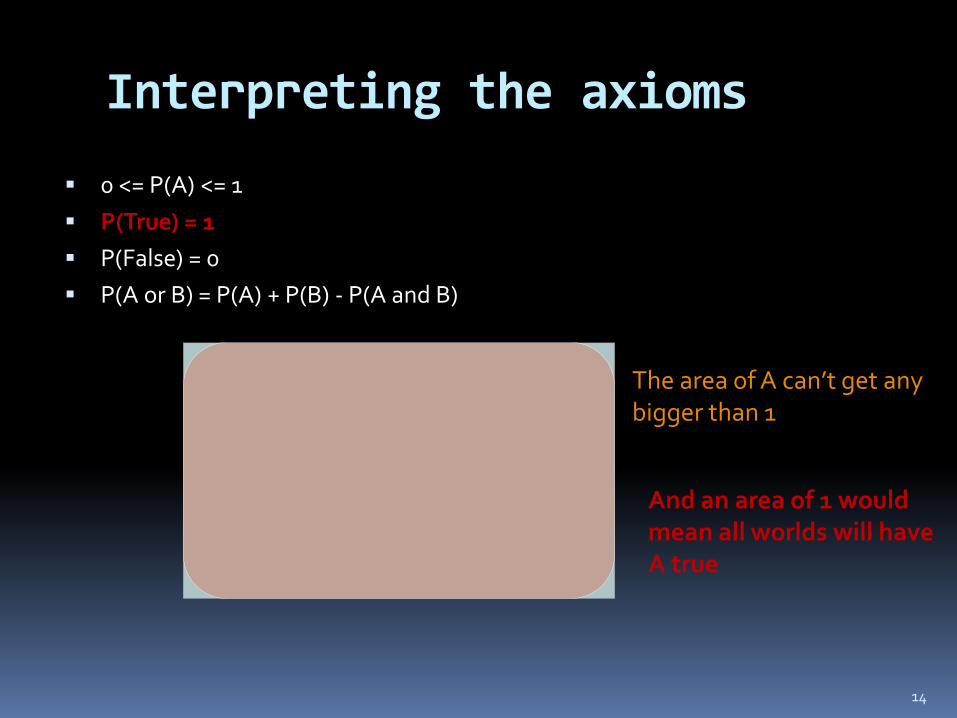
Interpreting the axioms
0 <= P(A) <= 1
P(True) = 1
P(False) = 0
P(A or B) = P(A) + P(B) - P(A and B)
14
The area of A can’t get any bigger than 1
And an area of 1 would mean all worlds will have A true
A
B
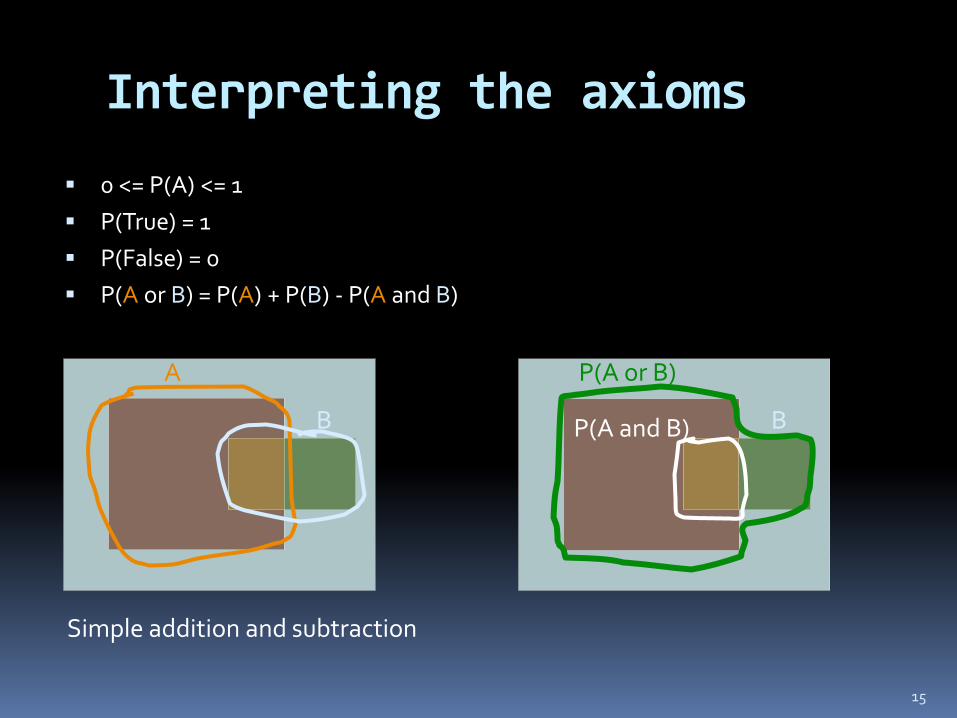
Interpreting the axioms
0 <= P(A) <= 1
P(True) = 1
P(False) = 0
P(A or B) = P(A) + P(B) - P(A and B)
15
P(A or B)
B P(A and B)
Simple addition and subtraction
Another Important Theorem
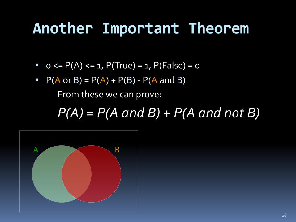
0 <= P(A) <= 1, P(True) = 1, P(False) = 0
P(A or B) = P(A) + P(B) - P(A and B)
From these we can prove:
P(A) = P(A and B) + P(A and not B)
16
A B
Conditional Probability
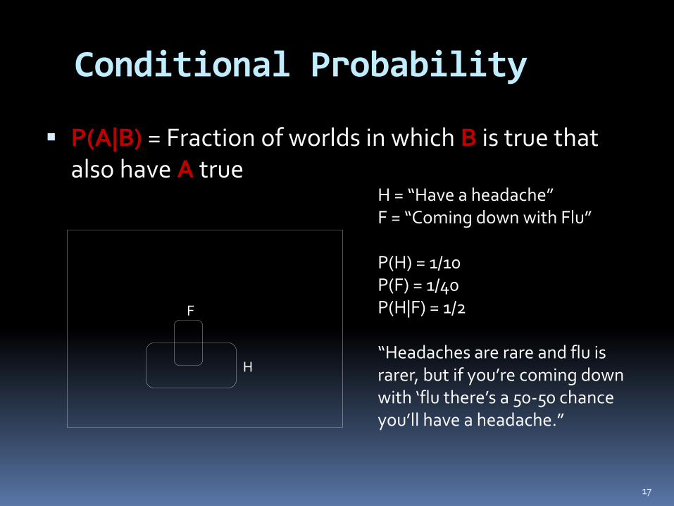
P(A|B) = Fraction of worlds in which B is true that also have A true
17
F
H
H = “Have a headache” F = “Coming down with Flu” P(H) = 1/10 P(F) = 1/40 P(H|F) = 1/2 “Headaches are rare and flu is rarer, but if you’re coming down with ‘flu there’s a 50-50 chance you’ll have a headache.”
Conditional Probability
18
F
H
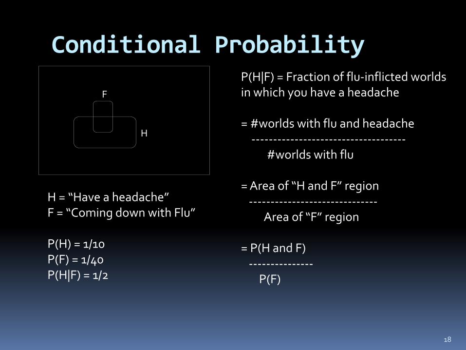
H = “Have a headache” F = “Coming down with Flu” P(H) = 1/10 P(F) = 1/40 P(H|F) = 1/2
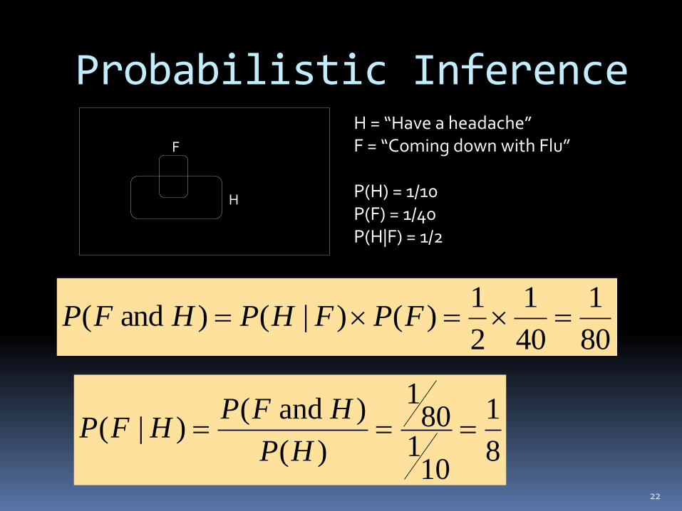
P(H|F) = Fraction of flu-inflicted worlds in which you have a headache = #worlds with flu and headache ------------------------------------ #worlds with flu = Area of “H and F” region ------------------------------ Area of “F” region = P(H and F) --------------- P(F)
Definition of Conditional Probability
19
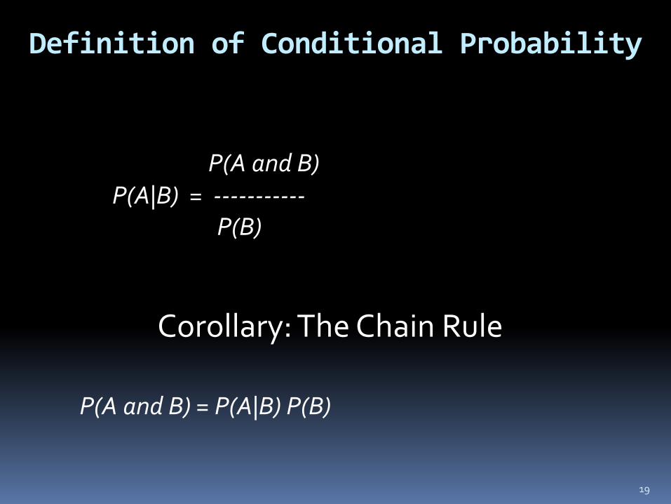
P(A and B) P(A|B) = ----------- P(B)
Corollary: The Chain Rule
P(A and B) = P(A|B) P(B)
Probabilistic Inference
20
F
H
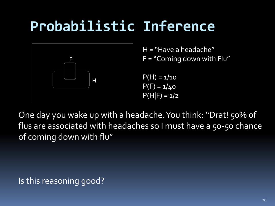
H = “Have a headache” F = “Coming down with Flu” P(H) = 1/10 P(F) = 1/40 P(H|F) = 1/2
One day you wake up with a headache. You think: “Drat! 50% of flus are associated with headaches so I must have a 50-50 chance of coming down with flu” Is this reasoning good?
Probabilistic Inference
21
F
H
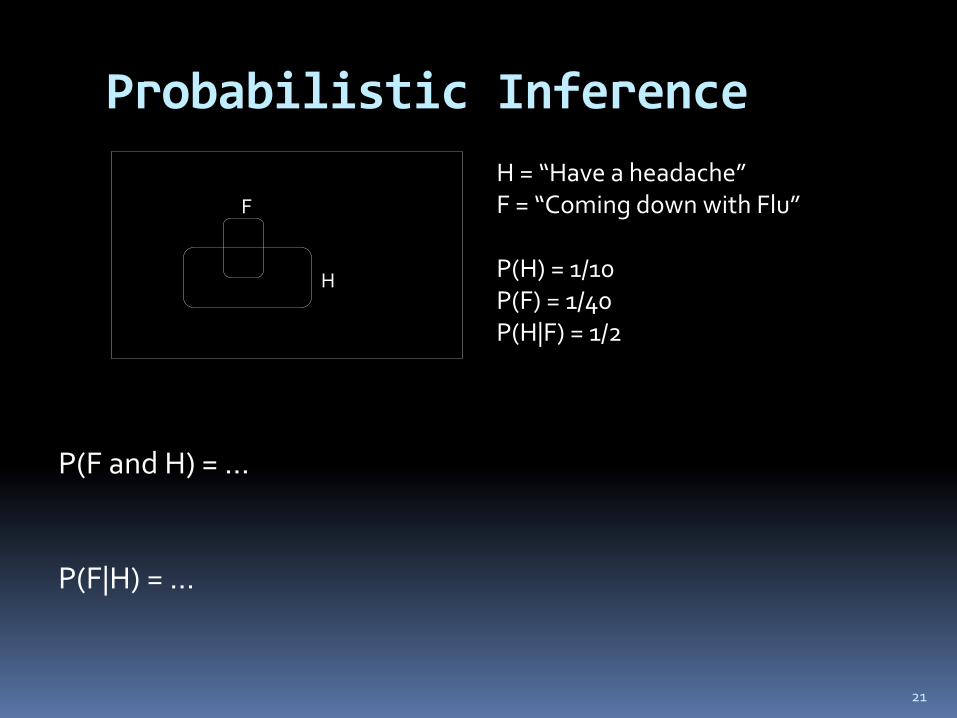
H = “Have a headache” F = “Coming down with Flu” P(H) = 1/10 P(F) = 1/40 P(H|F) = 1/2
P(F and H) = … P(F|H) = …
Probabilistic Inference
22
F
H
H = “Have a headache” F = “Coming down with Flu” P(H) = 1/10 P(F) = 1/40 P(H|F) = 1/2
8
1
10180
1
)(
) and ()|(
HP
HFPHFP
80
1
40
1
2
1)()|() and ( FPFHPHFP
What we just did…
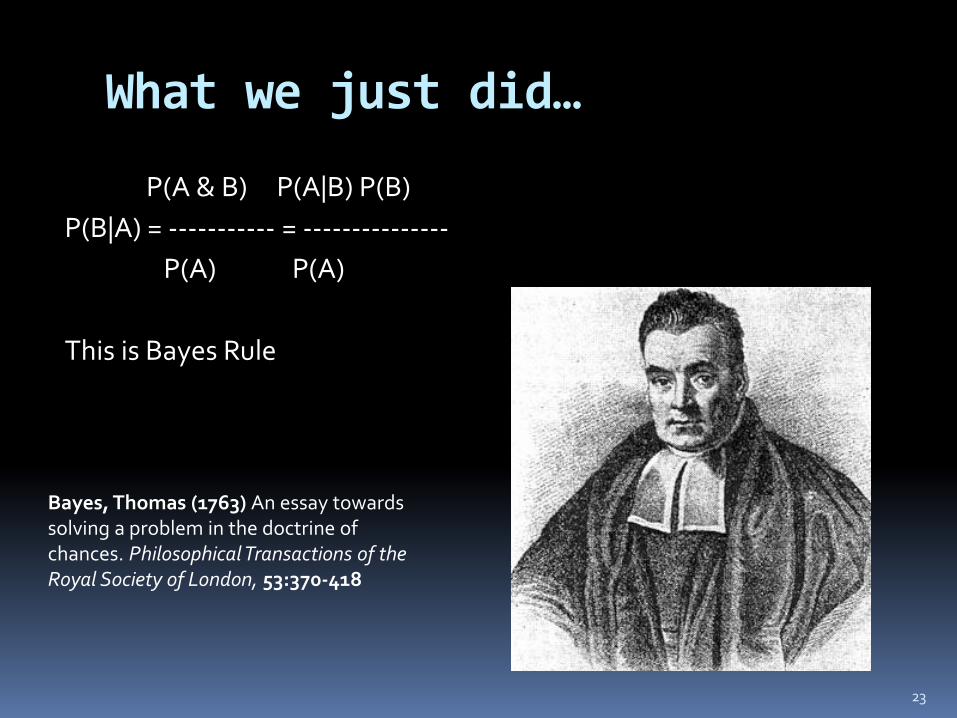
P(A & B) P(A|B) P(B)
P(B|A) = ----------- = ---------------
P(A) P(A)
This is Bayes Rule
23
Bayes, Thomas (1763) An essay towards solving a problem in the doctrine of chances. Philosophical Transactions of the Royal Society of London, 53:370-418
More Terminology
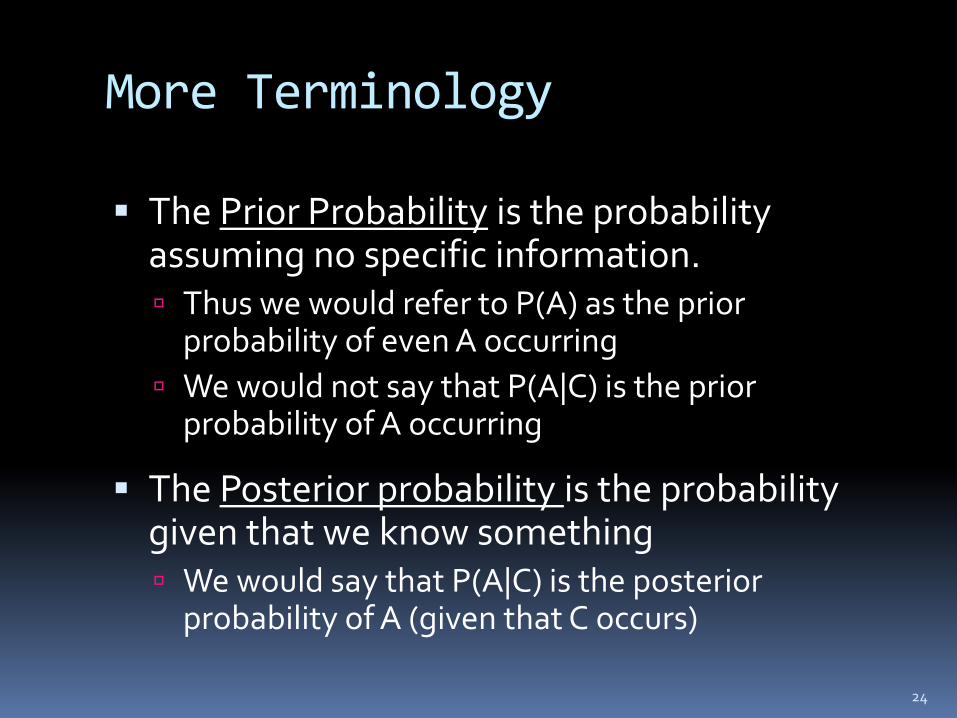
The Prior Probability is the probability assuming no specific information. Thus we would refer to P(A) as the prior
probability of even A occurring
We would not say that P(A|C) is the prior probability of A occurring
The Posterior probability is the probability given that we know something We would say that P(A|C) is the posterior
probability of A (given that C occurs)
24
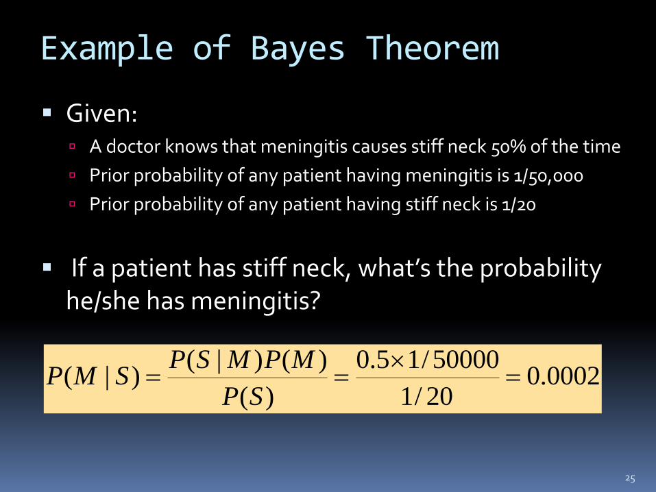
Example of Bayes Theorem
Given: A doctor knows that meningitis causes stiff neck 50% of the time
Prior probability of any patient having meningitis is 1/50,000
Prior probability of any patient having stiff neck is 1/20
If a patient has stiff neck, what’s the probability he/she has meningitis?
25
0002.020/1
50000/15.0
)(
)()|()|(
SP
MPMSPSMP
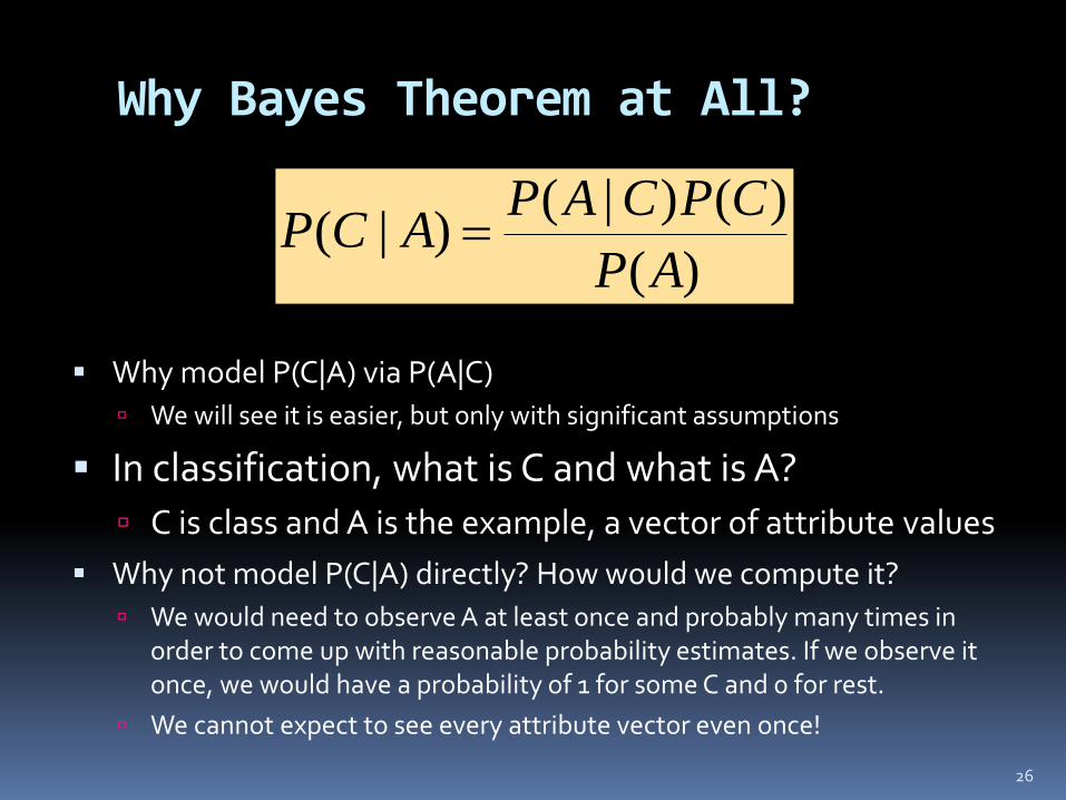
Why Bayes Theorem at All?
Why model P(C|A) via P(A|C)
We will see it is easier, but only with significant assumptions
In classification, what is C and what is A?
C is class and A is the example, a vector of attribute values
Why not model P(C|A) directly? How would we compute it?
We would need to observe A at least once and probably many times in order to come up with reasonable probability estimates. If we observe it once, we would have a probability of 1 for some C and 0 for rest.
We cannot expect to see every attribute vector even once!
26
)(
)()|()|(
AP
CPCAPACP
Bayes Classifiers
27
That was a visual intuition for a simple case of the Bayes classifier, also called:
• Idiot Bayes • Naïve Bayes • Simple Bayes
We are about to see some of the mathematical formalisms, and more examples, but keep in mind the basic idea. Find out the probability of the previously unseen instance belonging to each class, then simply pick the most probable class.

Bayesian Classifiers
Bayesian classifiers use Bayes theorem, which says
p(cj | d ) = p(d | cj ) p(cj)
p(d) p(cj | d) = probability of instance d being in class cj,
This is what we are trying to compute
p(d | cj) = probability of generating instance d given class cj,
We can imagine that being in class cj, causes you to have feature d with some probability
p(cj) = probability of occurrence of class cj,
This is just how frequent the class cj, is in our database
p(d) = probability of instance d occurring This can actually be ignored, since it is the same for all classes
28
Bayesian Classifiers
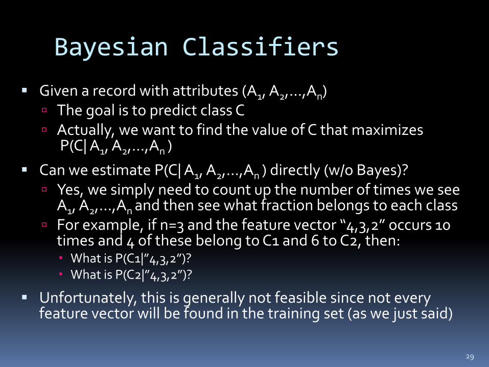
Given a record with attributes (A1, A2,…,An) The goal is to predict class C Actually, we want to find the value of C that maximizes
P(C| A1, A2,…,An )
Can we estimate P(C| A1, A2,…,An ) directly (w/o Bayes)? Yes, we simply need to count up the number of times we see
A1, A2,…,An and then see what fraction belongs to each class For example, if n=3 and the feature vector “4,3,2” occurs 10
times and 4 of these belong to C1 and 6 to C2, then: What is P(C1|”4,3,2”)? What is P(C2|”4,3,2”)?
Unfortunately, this is generally not feasible since not every feature vector will be found in the training set (as we just said)
29
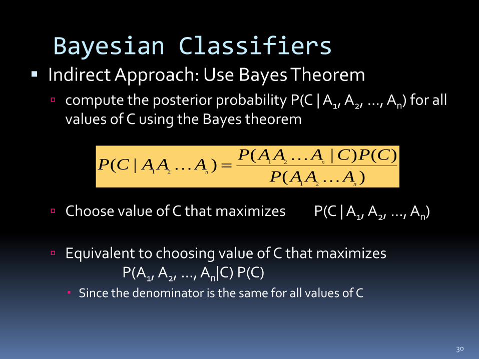
Bayesian Classifiers Indirect Approach: Use Bayes Theorem
compute the posterior probability P(C | A1, A2, …, An) for all values of C using the Bayes theorem
Choose value of C that maximizes P(C | A1, A2, …, An)
Equivalent to choosing value of C that maximizes P(A1, A2, …, An|C) P(C) Since the denominator is the same for all values of C
30
)(
)()|()|(
21
21
21
n
n
n
AAAP
CPCAAAPAAACP
Naïve Bayes Classifier
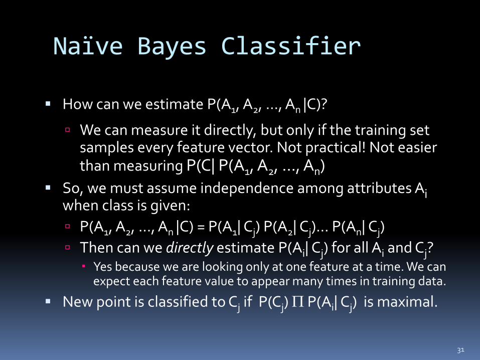
How can we estimate P(A1, A2, …, An |C)?
We can measure it directly, but only if the training set samples every feature vector. Not practical! Not easier than measuring P(C| P(A1, A2, …, An)
So, we must assume independence among attributes Ai when class is given:
P(A1, A2, …, An |C) = P(A1| Cj) P(A2| Cj)… P(An| Cj)
Then can we directly estimate P(Ai| Cj) for all Ai and Cj? Yes because we are looking only at one feature at a time. We can
expect each feature value to appear many times in training data.
New point is classified to Cj if P(Cj) P(Ai| Cj) is maximal.
31
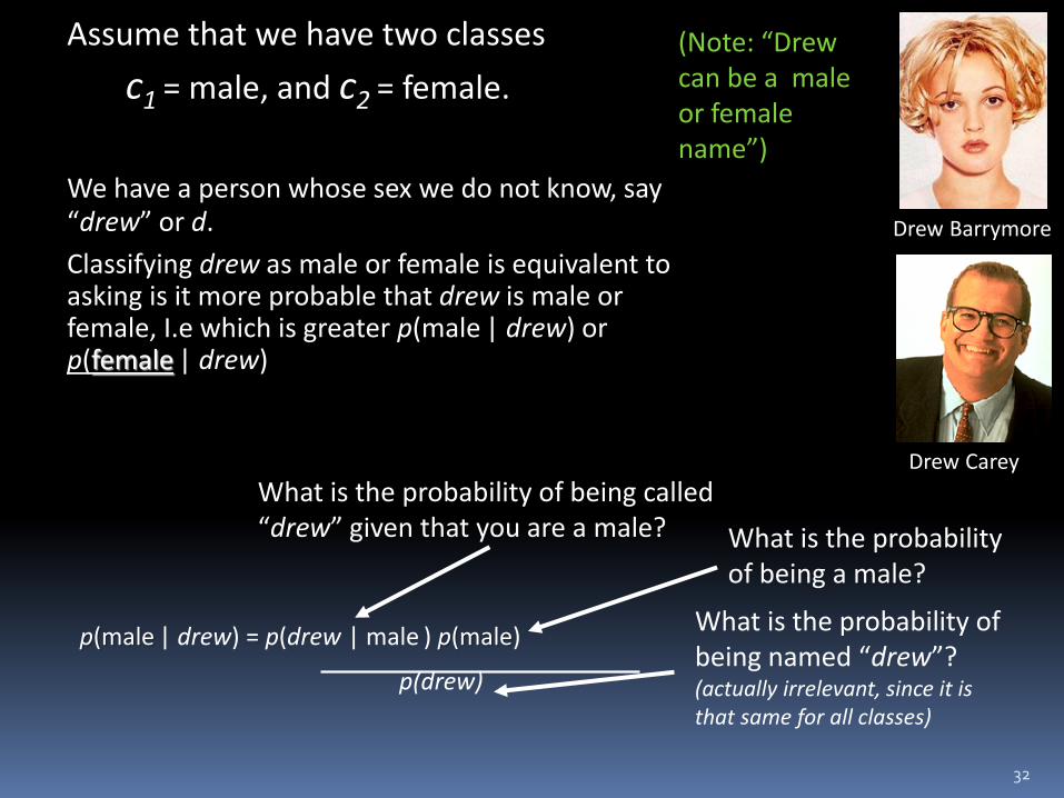
Assume that we have two classes
c1 = male, and c2 = female.
We have a person whose sex we do not know, say “drew” or d.
Classifying drew as male or female is equivalent to asking is it more probable that drew is male or female, I.e which is greater p(male | drew) or p(female | drew)
32
p(male | drew) = p(drew | male ) p(male)
p(drew)
(Note: “Drew can be a male or female name”)
What is the probability of being called “drew” given that you are a male? What is the probability
of being a male?
What is the probability of being named “drew”? (actually irrelevant, since it is that same for all classes)
Drew Carey
Drew Barrymore
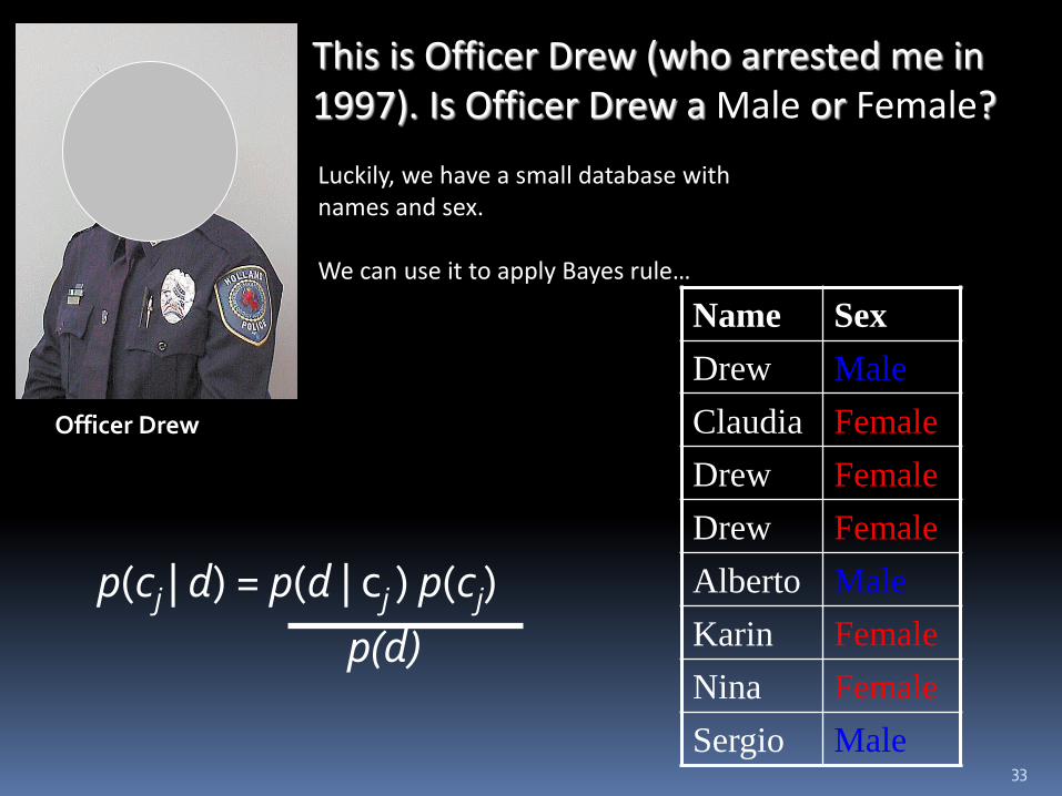
p(cj | d) = p(d | cj ) p(cj)
p(d)
Officer Drew
Name Sex
Drew Male
Claudia Female
Drew Female
Drew Female
Alberto Male
Karin Female
Nina Female
Sergio Male
This is Officer Drew (who arrested me in 1997). Is Officer Drew a Male or Female?
Luckily, we have a small database with names and sex. We can use it to apply Bayes rule…
33
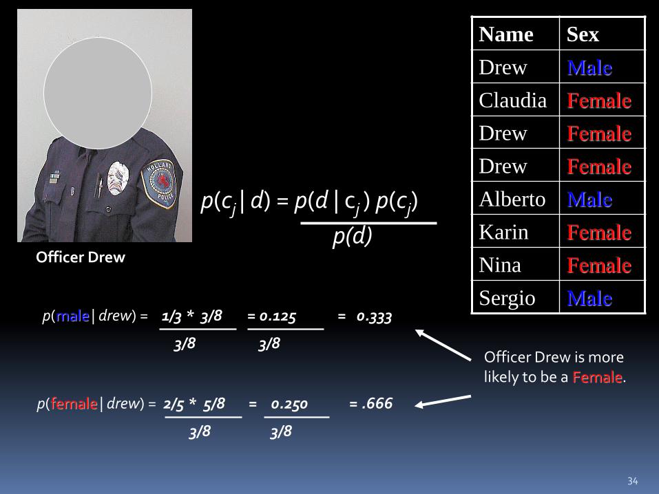
p(male | drew) = 1/3 * 3/8 = 0.125 = 0.333
3/8 3/8
p(female | drew) = 2/5 * 5/8 = 0.250 = .666
3/8 3/8
Officer Drew
p(cj | d) = p(d | cj ) p(cj)
p(d)
Name Sex
Drew Male
Claudia Female
Drew Female
Drew Female
Alberto Male
Karin Female
Nina Female
Sergio Male
Officer Drew is more likely to be a Female.
34
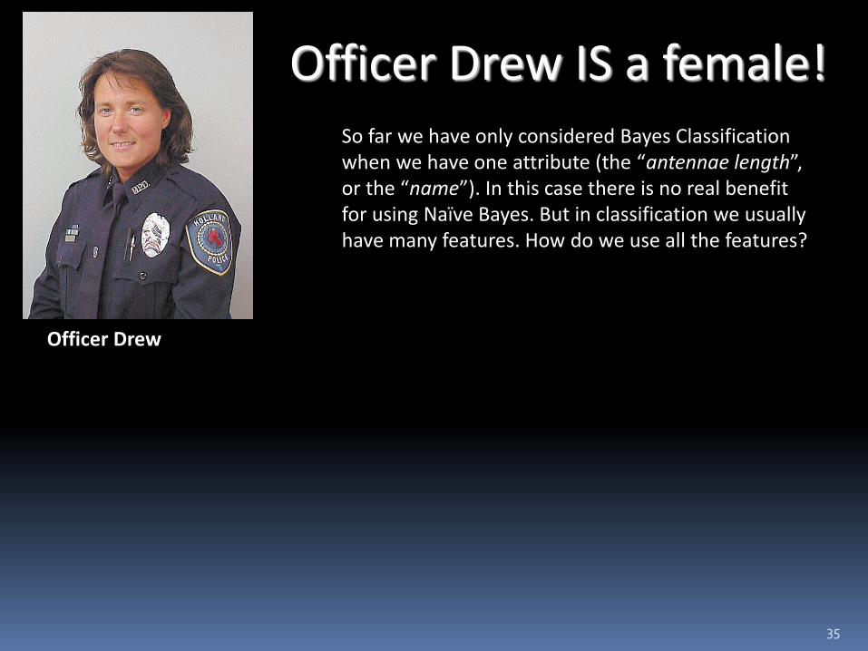
Officer Drew IS a female!
Officer Drew
So far we have only considered Bayes Classification when we have one attribute (the “antennae length”, or the “name”). In this case there is no real benefit for using Naïve Bayes. But in classification we usually have many features. How do we use all the features?
35
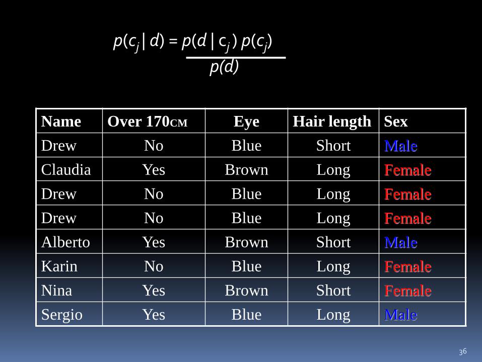
36
Name Over 170CM Eye Hair length Sex
Drew No Blue Short Male
Claudia Yes Brown Long Female
Drew No Blue Long Female
Drew No Blue Long Female
Alberto Yes Brown Short Male
Karin No Blue Long Female
Nina Yes Brown Short Female
Sergio Yes Blue Long Male
p(cj | d) = p(d | cj ) p(cj)
p(d)
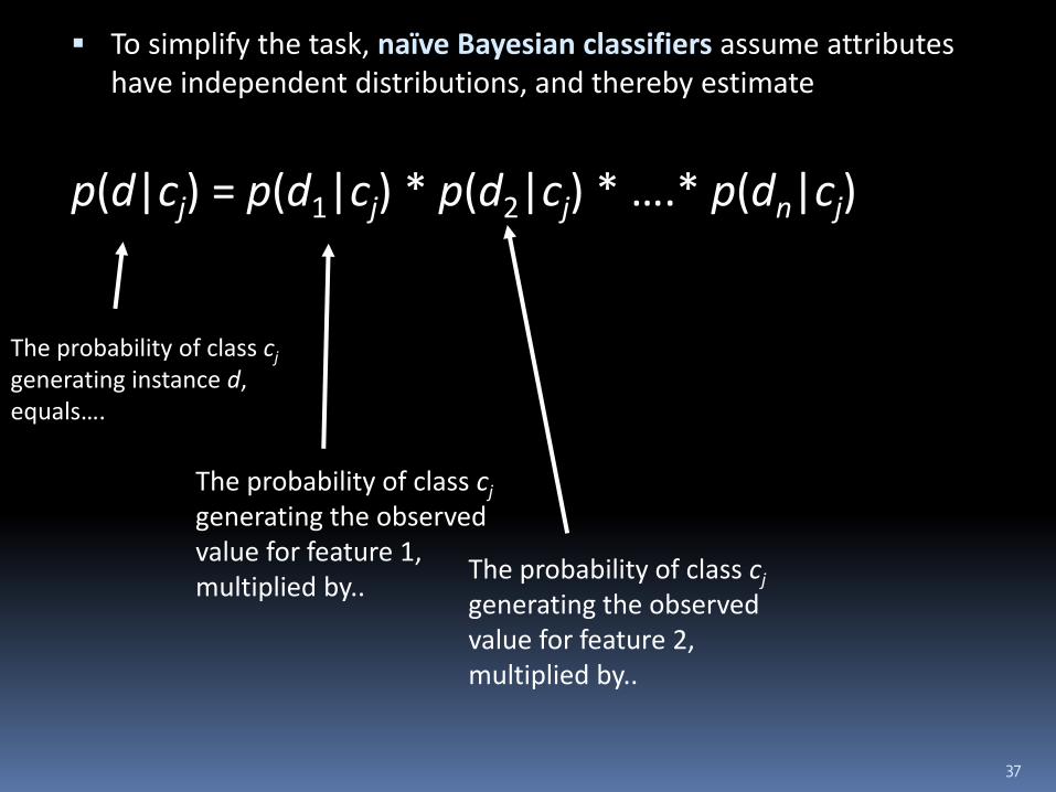
To simplify the task, naïve Bayesian classifiers assume attributes have independent distributions, and thereby estimate
p(d|cj) = p(d1|cj) * p(d2|cj) * ….* p(dn|cj)
37
The probability of class cj generating instance d, equals….
The probability of class cj generating the observed value for feature 1, multiplied by..
The probability of class cj generating the observed value for feature 2, multiplied by..
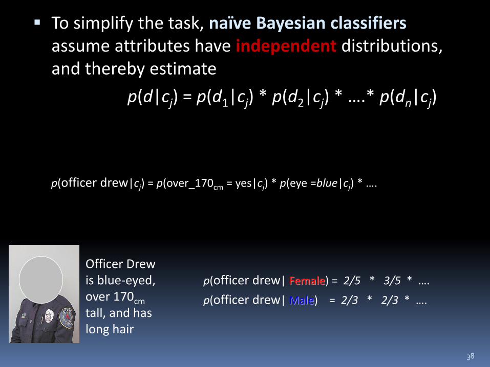
To simplify the task, naïve Bayesian classifiers assume attributes have independent distributions, and thereby estimate
p(d|cj) = p(d1|cj) * p(d2|cj) * ….* p(dn|cj)
38
p(officer drew|cj) = p(over_170cm = yes|cj) * p(eye =blue|cj) * ….
Officer Drew is blue-eyed, over 170cm tall, and has long hair
p(officer drew| Female) = 2/5 * 3/5 * ….
p(officer drew| Male) = 2/3 * 2/3 * ….
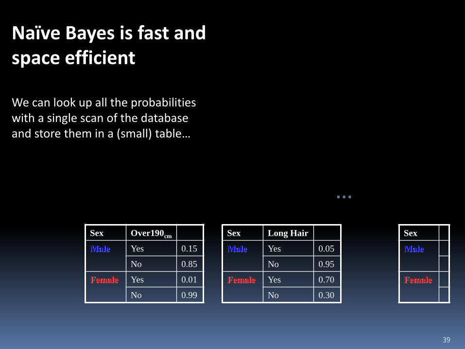
Naïve Bayes is fast and space efficient We can look up all the probabilities with a single scan of the database and store them in a (small) table…
Sex Over190cm
Male Yes 0.15
No 0.85
Female Yes 0.01
No 0.99
…
39
Sex Long Hair
Male Yes 0.05
No 0.95
Female Yes 0.70
No 0.30
Sex
Male
Female
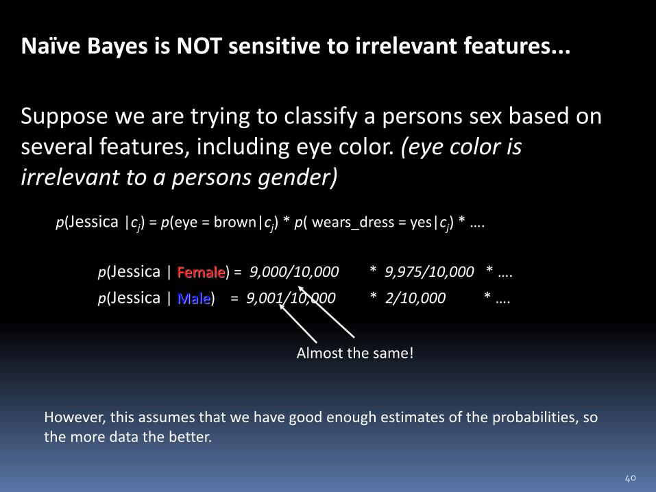
Naïve Bayes is NOT sensitive to irrelevant features...
Suppose we are trying to classify a persons sex based on several features, including eye color. (eye color is irrelevant to a persons gender)
p(Jessica | Female) = 9,000/10,000 * 9,975/10,000 * ….
p(Jessica | Male) = 9,001/10,000 * 2/10,000 * ….
p(Jessica |cj) = p(eye = brown|cj) * p( wears_dress = yes|cj) * ….
However, this assumes that we have good enough estimates of the probabilities, so the more data the better.
Almost the same!
40
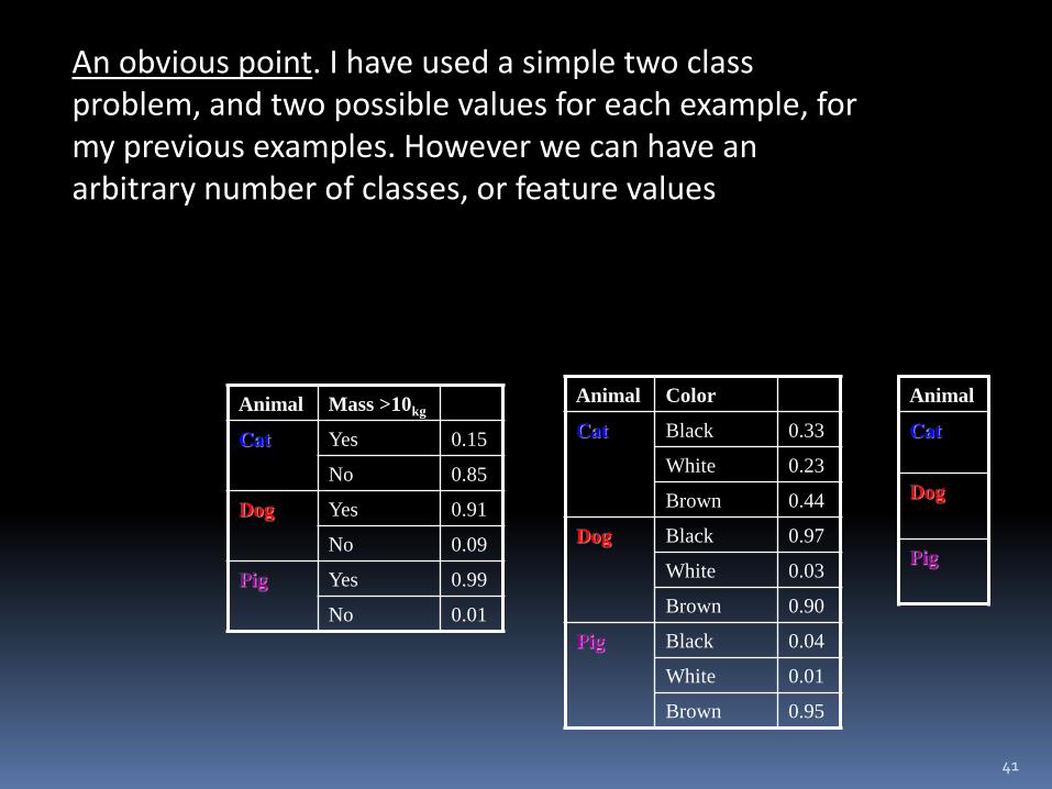
An obvious point. I have used a simple two class problem, and two possible values for each example, for my previous examples. However we can have an arbitrary number of classes, or feature values
Animal Mass >10kg
Cat Yes 0.15
No 0.85
Dog Yes 0.91
No 0.09
Pig Yes 0.99
No 0.01
41
Animal
Cat
Dog
Pig
Animal Color
Cat Black 0.33
White 0.23
Brown 0.44
Dog Black 0.97
White 0.03
Brown 0.90
Pig Black 0.04
White 0.01
Brown 0.95
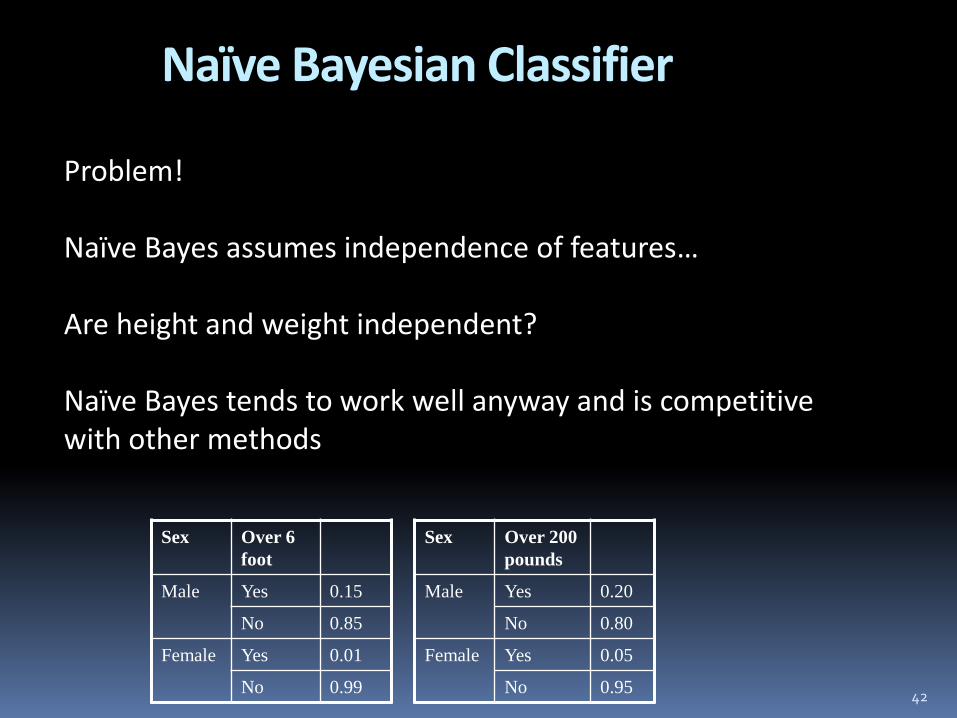
Naïve Bayesian Classifier
42
Problem! Naïve Bayes assumes independence of features… Are height and weight independent? Naïve Bayes tends to work well anyway and is competitive with other methods
Sex Over 6
foot
Male Yes 0.15
No 0.85
Female Yes 0.01
No 0.99
Sex Over 200
pounds
Male Yes 0.20
No 0.80
Female Yes 0.05
No 0.95

43
10
1 2 3 4 5 6 7 8 9 10
1
2
3
4
5
6
7
8
9
The Naïve Bayesian Classifier has a quadratic decision boundary
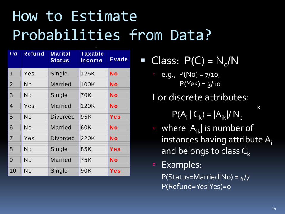
How to Estimate Probabilities from Data?
Class: P(C) = Nc/N e.g., P(No) = 7/10,
P(Yes) = 3/10
For discrete attributes:
P(Ai | Ck) = |Aik|/ Nc
where |Aik| is number of instances having attribute Ai and belongs to class Ck
Examples: P(Status=Married|No) = 4/7
P(Refund=Yes|Yes)=0
44
k
Tid Refund Marital Status
Taxable Income Evade
1 Yes Single 125K No
2 No Married 100K No
3 No Single 70K No
4 Yes Married 120K No
5 No Divorced 95K Yes
6 No Married 60K No
7 Yes Divorced 220K No
8 No Single 85K Yes
9 No Married 75K No
10 No Single 90K Yes 10
categoric
al
categoric
al
continuous
class
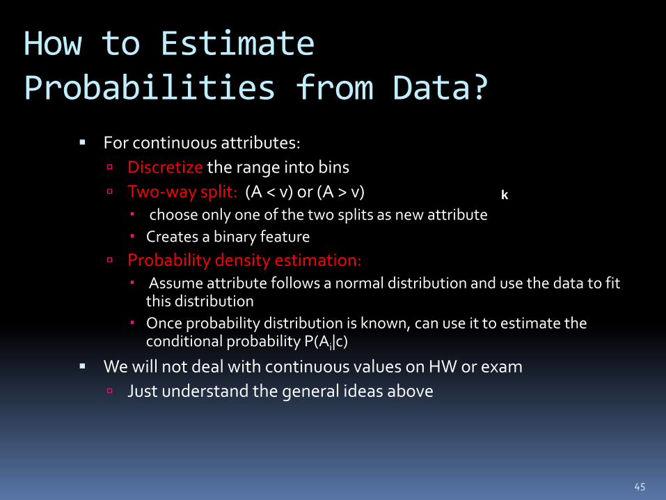
How to Estimate Probabilities from Data?
For continuous attributes:
Discretize the range into bins
Two-way split: (A < v) or (A > v) choose only one of the two splits as new attribute
Creates a binary feature
Probability density estimation: Assume attribute follows a normal distribution and use the data to fit
this distribution
Once probability distribution is known, can use it to estimate the conditional probability P(Ai|c)
We will not deal with continuous values on HW or exam
Just understand the general ideas above
45
k
Example of Naïve Bayes
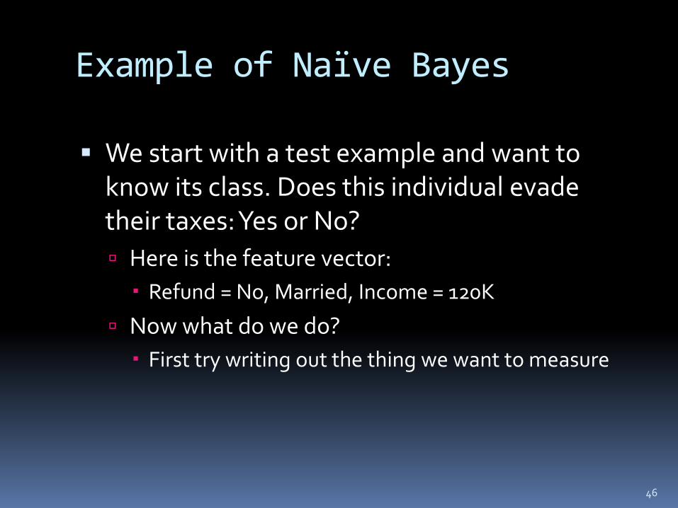
We start with a test example and want to know its class. Does this individual evade their taxes: Yes or No?
Here is the feature vector:
Refund = No, Married, Income = 120K
Now what do we do?
First try writing out the thing we want to measure
46
Example of Naïve Bayes
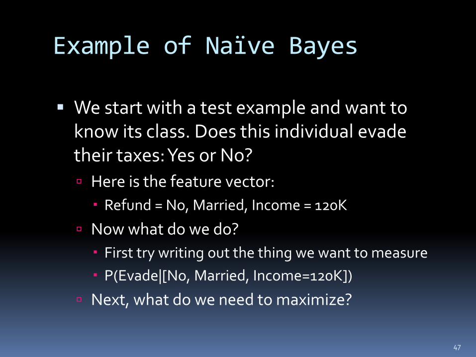
We start with a test example and want to know its class. Does this individual evade their taxes: Yes or No?
Here is the feature vector:
Refund = No, Married, Income = 120K
Now what do we do?
First try writing out the thing we want to measure
P(Evade|[No, Married, Income=120K])
Next, what do we need to maximize?
47
Example of Naïve Bayes
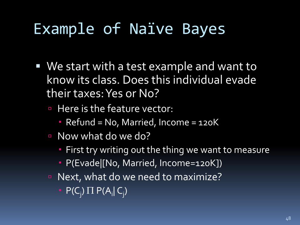
We start with a test example and want to know its class. Does this individual evade their taxes: Yes or No? Here is the feature vector:
Refund = No, Married, Income = 120K
Now what do we do? First try writing out the thing we want to measure
P(Evade|[No, Married, Income=120K])
Next, what do we need to maximize? P(Cj) P(Ai| Cj)
48
Example of Naïve Bayes
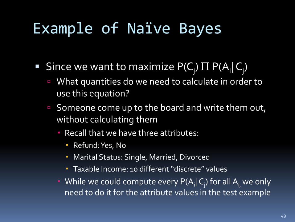
Since we want to maximize P(Cj) P(Ai| Cj)
What quantities do we need to calculate in order to use this equation?
Someone come up to the board and write them out, without calculating them
Recall that we have three attributes:
Refund: Yes, No
Marital Status: Single, Married, Divorced
Taxable Income: 10 different “discrete” values
While we could compute every P(Ai| Cj) for all Ai, we only need to do it for the attribute values in the test example
49
Values to Compute
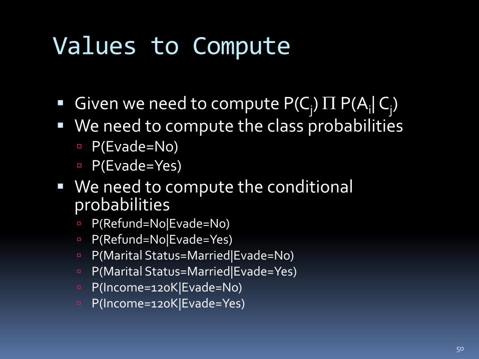
Given we need to compute P(Cj) P(Ai| Cj) We need to compute the class probabilities
P(Evade=No) P(Evade=Yes)
We need to compute the conditional probabilities P(Refund=No|Evade=No) P(Refund=No|Evade=Yes) P(Marital Status=Married|Evade=No) P(Marital Status=Married|Evade=Yes) P(Income=120K|Evade=No) P(Income=120K|Evade=Yes)
50

Computed Values
Given we need to compute P(Cj) P(Ai| Cj) We need to compute the class probabilities
P(Evade=No) = 7/10 = .7 P(Evade=Yes) = 3/10 = .3
We need to compute the conditional probabilities P(Refund=No|Evade=No) = 4/7 P(Refund=No|Evade=Yes) 3/3 = 1.0 P(Marital Status=Married|Evade=No) = 4/7 P(Marital Status=Married|Evade=Yes) =0/3 = 0 P(Income=120K|Evade=No) = 1/7 P(Income=120K|Evade=Yes) = 0/7 = 0
51
Finding the Class
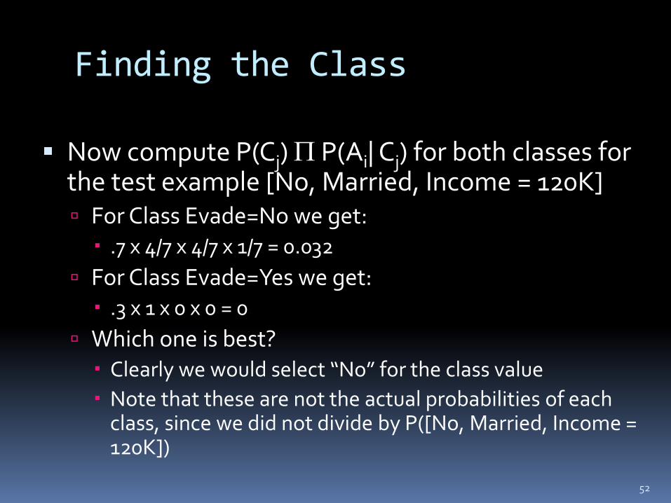
Now compute P(Cj) P(Ai| Cj) for both classes for the test example [No, Married, Income = 120K] For Class Evade=No we get:
.7 x 4/7 x 4/7 x 1/7 = 0.032
For Class Evade=Yes we get: .3 x 1 x 0 x 0 = 0
Which one is best? Clearly we would select “No” for the class value
Note that these are not the actual probabilities of each class, since we did not divide by P([No, Married, Income = 120K])
52
Naïve Bayes Classifier
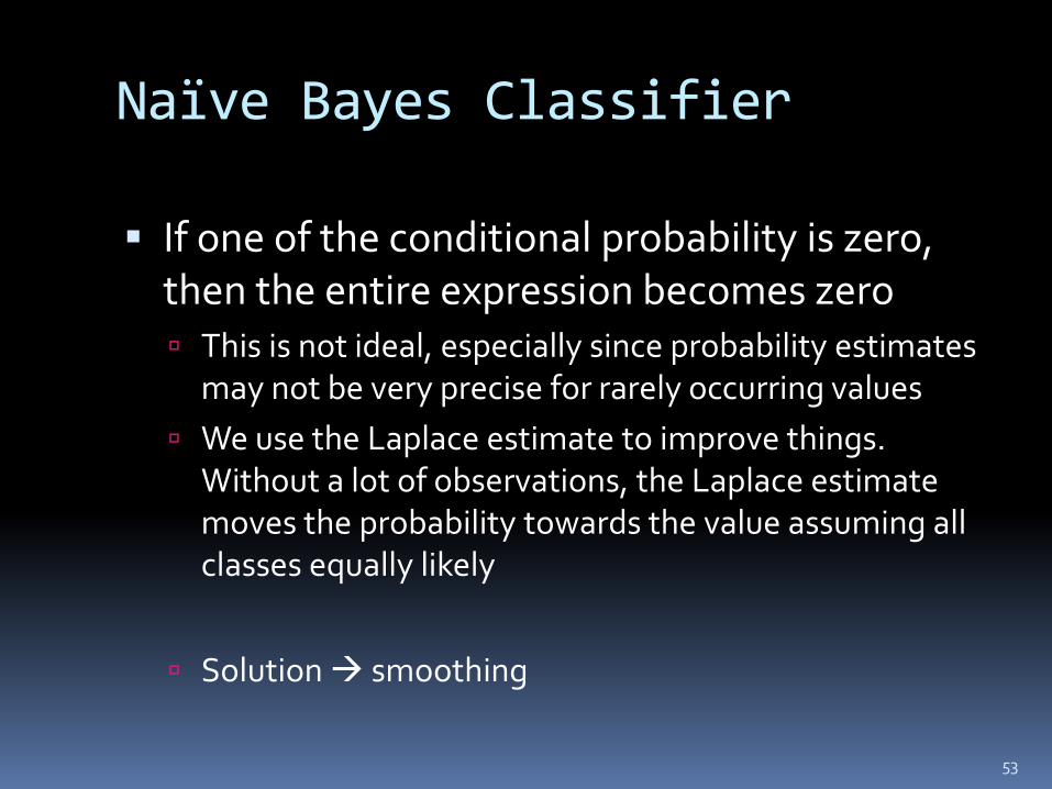
If one of the conditional probability is zero, then the entire expression becomes zero This is not ideal, especially since probability estimates
may not be very precise for rarely occurring values
We use the Laplace estimate to improve things. Without a lot of observations, the Laplace estimate moves the probability towards the value assuming all classes equally likely
Solution smoothing
53
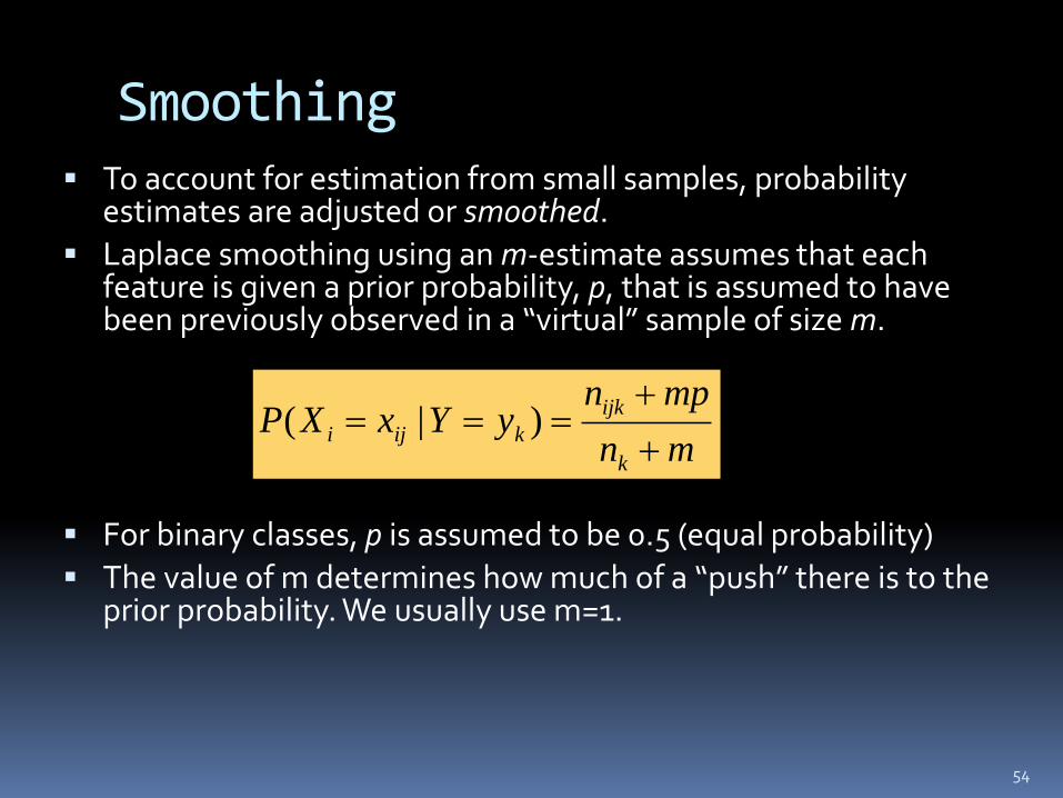
Smoothing To account for estimation from small samples, probability
estimates are adjusted or smoothed.
Laplace smoothing using an m-estimate assumes that each feature is given a prior probability, p, that is assumed to have been previously observed in a “virtual” sample of size m.
For binary classes, p is assumed to be 0.5 (equal probability)
The value of m determines how much of a “push” there is to the prior probability. We usually use m=1.
54
mn
mpnyYxXP
k
ijk
kiji
)|(
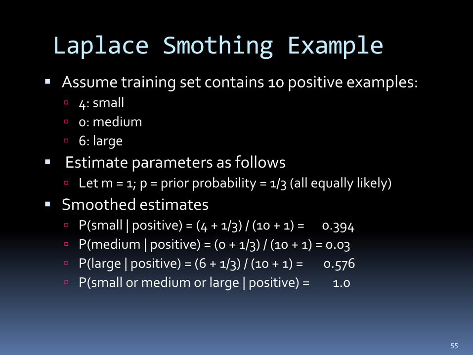
Laplace Smothing Example
Assume training set contains 10 positive examples: 4: small
0: medium
6: large
Estimate parameters as follows Let m = 1; p = prior probability = 1/3 (all equally likely)
Smoothed estimates P(small | positive) = (4 + 1/3) / (10 + 1) = 0.394
P(medium | positive) = (0 + 1/3) / (10 + 1) = 0.03
P(large | positive) = (6 + 1/3) / (10 + 1) = 0.576
P(small or medium or large | positive) = 1.0
55
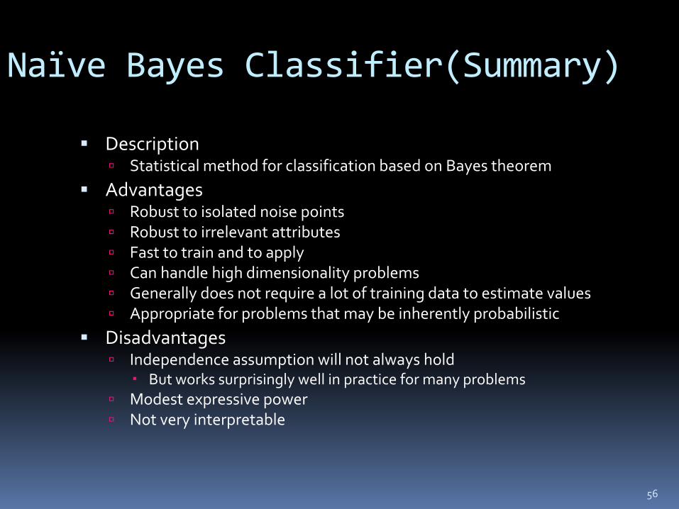
Naïve Bayes Classifier(Summary)
Description Statistical method for classification based on Bayes theorem
Advantages Robust to isolated noise points Robust to irrelevant attributes Fast to train and to apply Can handle high dimensionality problems Generally does not require a lot of training data to estimate values Appropriate for problems that may be inherently probabilistic
Disadvantages Independence assumption will not always hold
But works surprisingly well in practice for many problems
Modest expressive power Not very interpretable
56
More Examples
There are several detailed examples provided
Go over them before trying the HW, unless you are clear on Bayesian Classifiers
57

Play-tennis example: estimate P(xi|C)
Outlook Temperature Humidity Windy Class
sunny hot high false N
sunny hot high true N
overcast hot high false P
rain mild high false P
rain cool normal false P
rain cool normal true N
overcast cool normal true P
sunny mild high false N
sunny cool normal false P
rain mild normal false P
sunny mild normal true P
overcast mild high true P
overcast hot normal false P
rain mild high true N
outlook
P(sunny|p) = 2/9 P(sunny|n) = 3/5
P(overcast|p) = 4/9 P(overcast|n) = 0
P(rain|p) = 3/9 P(rain|n) = 2/5
Temperature
P(hot|p) = 2/9 P(hot|n) = 2/5
P(mild|p) = 4/9 P(mild|n) = 2/5
P(cool|p) = 3/9 P(cool|n) = 1/5
Humidity
P(high|p) = 3/9 P(high|n) = 4/5
P(normal|p) = 6/9 P(normal|n) = 2/5
windy
P(true|p) = 3/9 P(true|n) = 3/5
P(false|p) = 6/9 P(false|n) = 2/5
P(p) = 9/14
P(n) = 5/14
58
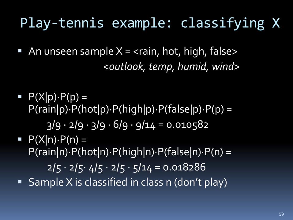
Play-tennis example: classifying X
An unseen sample X = <rain, hot, high, false>
<outlook, temp, humid, wind>
P(X|p)·P(p) = P(rain|p)·P(hot|p)·P(high|p)·P(false|p)·P(p) =
3/9 · 2/9 · 3/9 · 6/9 · 9/14 = 0.010582
P(X|n)·P(n) = P(rain|n)·P(hot|n)·P(high|n)·P(false|n)·P(n) =
2/5 · 2/5· 4/5 · 2/5 · 5/14 = 0.018286
Sample X is classified in class n (don’t play)
59
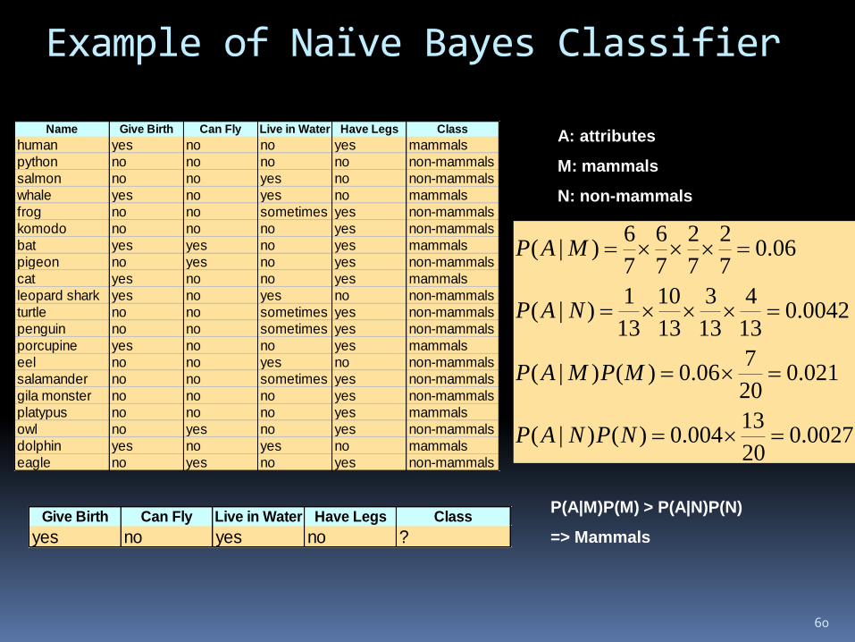
Example of Naïve Bayes Classifier
60
Name Give Birth Can Fly Live in Water Have Legs Class
human yes no no yes mammals
python no no no no non-mammals
salmon no no yes no non-mammals
whale yes no yes no mammals
frog no no sometimes yes non-mammals
komodo no no no yes non-mammals
bat yes yes no yes mammals
pigeon no yes no yes non-mammals
cat yes no no yes mammals
leopard shark yes no yes no non-mammals
turtle no no sometimes yes non-mammals
penguin no no sometimes yes non-mammals
porcupine yes no no yes mammals
eel no no yes no non-mammals
salamander no no sometimes yes non-mammals
gila monster no no no yes non-mammals
platypus no no no yes mammals
owl no yes no yes non-mammals
dolphin yes no yes no mammals
eagle no yes no yes non-mammals
Give Birth Can Fly Live in Water Have Legs Class
yes no yes no ?
0027.020
13004.0)()|(
021.020
706.0)()|(
0042.013
4
13
3
13
10
13
1)|(
06.07
2
7
2
7
6
7
6)|(
NPNAP
MPMAP
NAP
MAP
A: attributes
M: mammals
N: non-mammals
P(A|M)P(M) > P(A|N)P(N)
=> Mammals
61
• Advantages:
– Fast to train (single scan). Fast to classify
– Not sensitive to irrelevant features
– Handles real and discrete data
– Handles streaming data well
• Disadvantages:
– Assumes independence of features
Advantages/Disadvantages of Naïve Bayes