Embed Size (px)
Citation preview
Chloé-Agathe Azencott: Data Mining in Bioinformatics, Page 1
Data Mining in BioinformaticsDay 9: Graph Mining in Chemoinformatics
Chloé-Agathe Azencott & Karsten Borgwardt
February 18 to March 1, 2013
Machine Learning & Computational Biology Research GroupMax Planck Institutes Tübingen andEberhard Karls Universität Tübingen
Drug discovery
Chloé-Agathe Azencott: Data Mining in Bioinformatics, Page 2
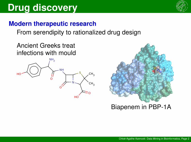
Modern therapeutic researchFrom serendipity to rationalized drug design
Ancient Greeks treatinfections with mould
CH 3
N
S
O
NH
O
HO
NH 2
O
HO
CH 3
Biapenem in PBP-1A
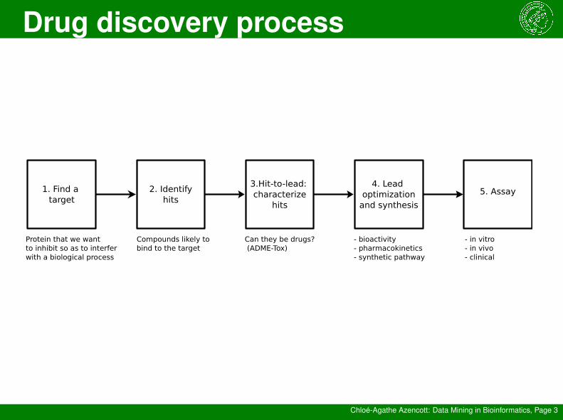
Drug discovery process
Chloé-Agathe Azencott: Data Mining in Bioinformatics, Page 3
1. Find a target
2. Identifyhits
3.Hit-to-lead: characterize
hits
4. Lead optimization
and synthesis
5. Assay
Protein that we want to inhibit so as to interfer with a biological process
Compounds likely to bind to the target
Can they be drugs? (ADME-Tox)
- in vitro- in vivo- clinical
- bioactivity- pharmacokinetics- synthetic pathway
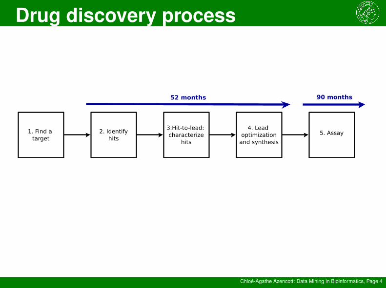
Drug discovery process
Chloé-Agathe Azencott: Data Mining in Bioinformatics, Page 4
52 months 90 months
1. Find a target
2. Identifyhits
3.Hit-to-lead: characterize
hits
4. Lead optimization
and synthesis
5. Assay
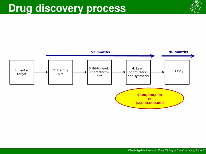
Drug discovery process
Chloé-Agathe Azencott: Data Mining in Bioinformatics, Page 5
$500,000,000to
$2,000,000,000
52 months 90 months
1. Find a target
2. Identifyhits
3.Hit-to-lead: characterize
hits
4. Lead optimization
and synthesis
5. Assay
Chemoinformatics
Chloé-Agathe Azencott: Data Mining in Bioinformatics, Page 6
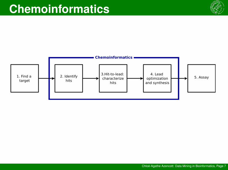
How can computer science help?→ Chemoinformatics!
“...the mixing of information resources to transform data into informa-tion, and information into knowledge, for the intended purpose of mak-ing better decisions faster in the arena of drug lead identification andoptimisation.” – F. K. Brown
“... the application of informatics methods to solve chemical problems.”– J. Gasteiger and T. Engel
Chemoinformatics
Chloé-Agathe Azencott: Data Mining in Bioinformatics, Page 7
Chemoinformatics
1. Find a target
2. Identifyhits
3.Hit-to-lead: characterize
hits
4. Lead optimization
and synthesis
5. Assay
Chemoinformatics
Chloé-Agathe Azencott: Data Mining in Bioinformatics, Page 8
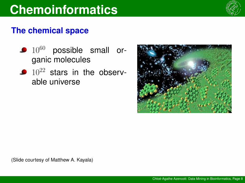
The chemical space
1060 possible small or-ganic molecules
1022 stars in the observ-able universe
(Slide courtesy of Matthew A. Kayala)
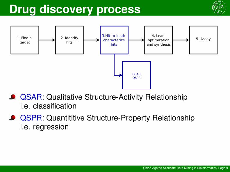
Drug discovery process
Chloé-Agathe Azencott: Data Mining in Bioinformatics, Page 9
QSARQSPR
1. Find a target
2. Identifyhits
3.Hit-to-lead: characterize
hits
4. Lead optimization
and synthesis
5. Assay
QSAR: Qualitative Structure-Activity Relationshipi.e. classification
QSPR: Quantititive Structure-Property Relationshipi.e. regression
Representing chemicals in silico
Chloé-Agathe Azencott: Data Mining in Bioinformatics, Page 10
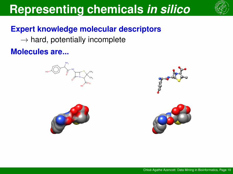
Expert knowledge molecular descriptors→ hard, potentially incomplete
Molecules are...
CH 3
N
S
O
NH
O
HO
NH 2
O
HO
CH 3
Representing chemicals in silico
Chloé-Agathe Azencott: Data Mining in Bioinformatics, Page 11
Similar Property PrincipleMolecules having similar structures should exhibit similaractivities.
→ Structure-based representationsCompare molecules by comparing substructures
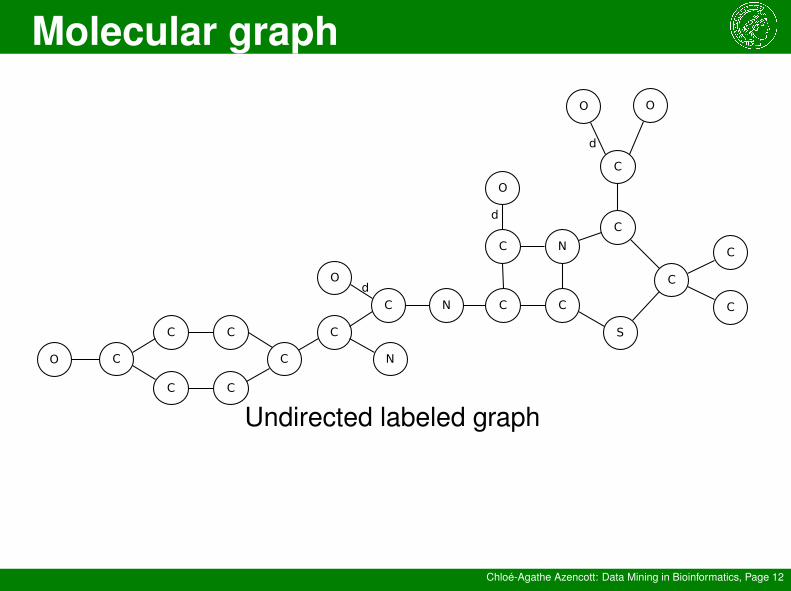
Molecular graph
Chloé-Agathe Azencott: Data Mining in Bioinformatics, Page 12
C
O
N C
C
C
N
O
S
C
C
O O
C
C
d
d
d
C
C
NC
C
C
C
C
CO
Undirected labeled graph
Fingerprints
Chloé-Agathe Azencott: Data Mining in Bioinformatics, Page 13
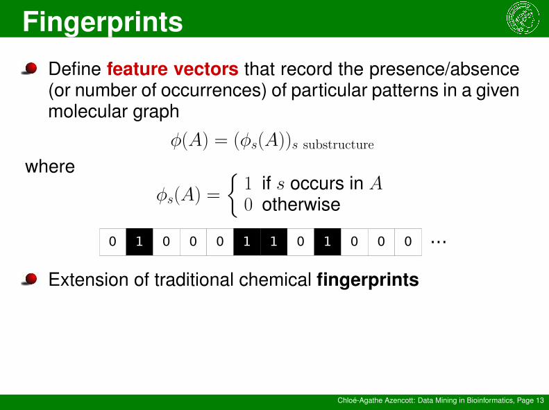
Define feature vectors that record the presence/absence(or number of occurrences) of particular patterns in a givenmolecular graph
φ(A) = (φs(A))s substructure
whereφs(A) =
{1 if s occurs in A0 otherwise
Extension of traditional chemical fingerprints
Fingerprints
Chloé-Agathe Azencott: Data Mining in Bioinformatics, Page 14
Learning from fingerprintsClassical machine learning and data mining techniquescan be applied to these vectorial feature representations.
Any distance / kernel can be usedClassificationFeature selectionClustering
Fingerprints
Chloé-Agathe Azencott: Data Mining in Bioinformatics, Page 15
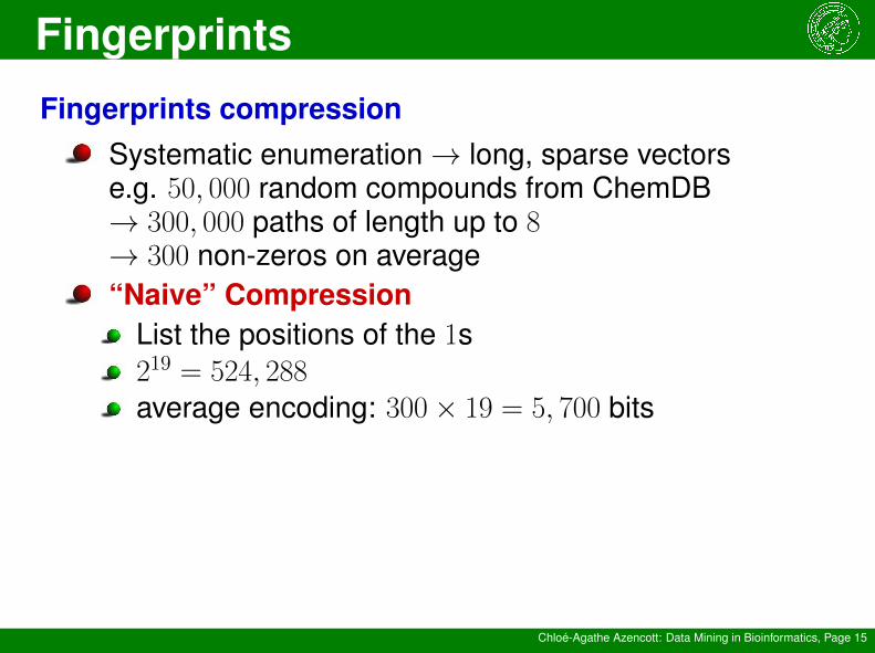
Fingerprints compressionSystematic enumeration→ long, sparse vectorse.g. 50, 000 random compounds from ChemDB→ 300, 000 paths of length up to 8→ 300 non-zeros on average“Naive” Compression
List the positions of the 1s219 = 524, 288average encoding: 300× 19 = 5, 700 bits
Fingerprints
Chloé-Agathe Azencott: Data Mining in Bioinformatics, Page 16
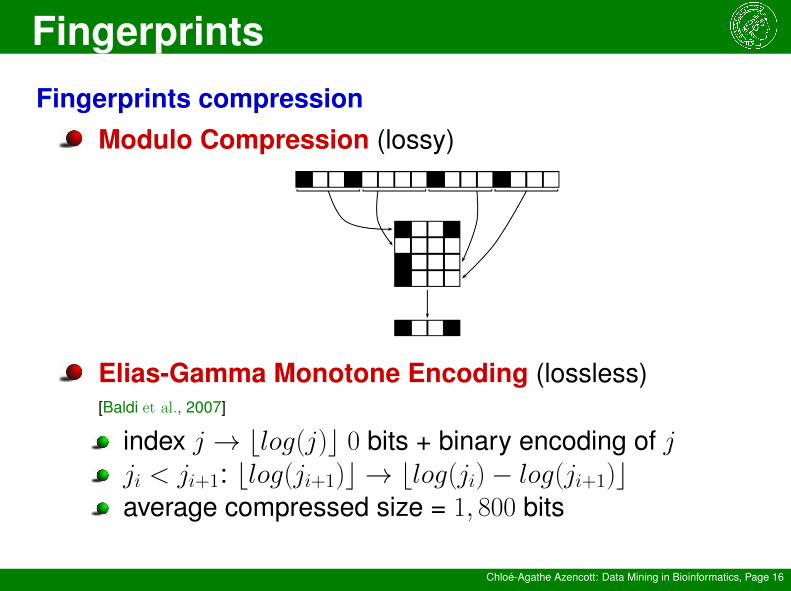
Fingerprints compressionModulo Compression (lossy)
Elias-Gamma Monotone Encoding (lossless)[Baldi et al., 2007]
index j → blog(j)c 0 bits + binary encoding of jji < ji+1: blog(ji+1)c → blog(ji)− log(ji+1)caverage compressed size = 1, 800 bits
Frequent patterns fingerprints
Chloé-Agathe Azencott: Data Mining in Bioinformatics, Page 17
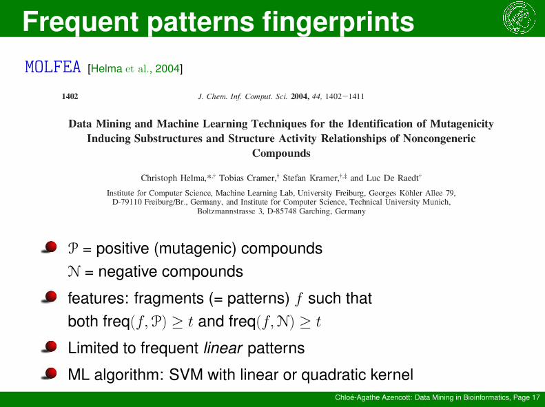
MOLFEA [Helma et al., 2004]
P = positive (mutagenic) compoundsN = negative compounds
features: fragments (= patterns) f such thatboth freq(f,P) ≥ t and freq(f,N) ≥ t
Limited to frequent linear patterns
ML algorithm: SVM with linear or quadratic kernel
Frequent patterns fingerprints
Chloé-Agathe Azencott: Data Mining in Bioinformatics, Page 18
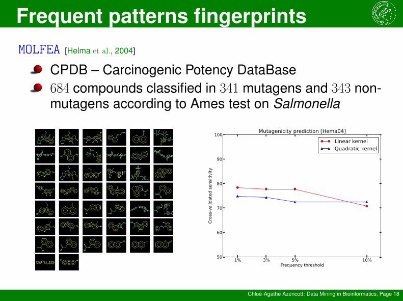
MOLFEA [Helma et al., 2004]
CPDB – Carcinogenic Potency DataBase684 compounds classified in 341 mutagens and 343 non-mutagens according to Ames test on Salmonella
1% 3% 5% 10%Frequency threshold
50
60
70
80
90
100
Cross-validated sensitivity
Mutagenicity prediction [Hema04]
Linear kernelQuadratic kernel
Spectrum kernels
Chloé-Agathe Azencott: Data Mining in Bioinformatics, Page 19
φ(A) = (φs(A))s∈S
Kspectrum(A,A′) = k(φ(A), φ(A′))
k ∈ RR|(S)|×R|(S)| can beDot product (linear kernel)
RBF kernel
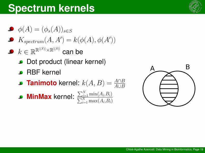
Tanimoto kernel: k(A,B) = A∩BA∪B
MinMax kernel:∑N
i=1min(Ai,Bi)∑Ni=1max(Ai,Bi)
Spectrum kernels
Chloé-Agathe Azencott: Data Mining in Bioinformatics, Page 20
Tanimoto and MinMaxBoth Tanimoto and Minmax are kernels.
Proof for Tanimoto: J.C. Gower A general coefficientof similarity and some of its properties. Biometrics1971.Proof for MinMax:
MinMax(x, y) =〈φ(x), φ(y)〉
〈φ(x), φ(x)〉 + 〈φ(y), φ(y)〉 − 〈φ(x), φ(y)〉with φ(x) of length: # patterns × max countφ(x)i = 1 iff. the pattern indexed by bi/qc appears morethan i mod q times in x
All patterns fingerprints
Chloé-Agathe Azencott: Data Mining in Bioinformatics, Page 21
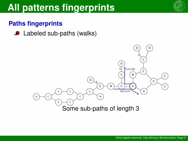
Paths fingerprintsLabeled sub-paths (walks)
O
N C C
N
O
S
C
C
O O
C
C
d
d
d
C
C
NsCsCsS
CsCsCdO
C
C
NC
C
C
C
C
CO
Some sub-paths of length 3
All patterns fingerprints
Chloé-Agathe Azencott: Data Mining in Bioinformatics, Page 22
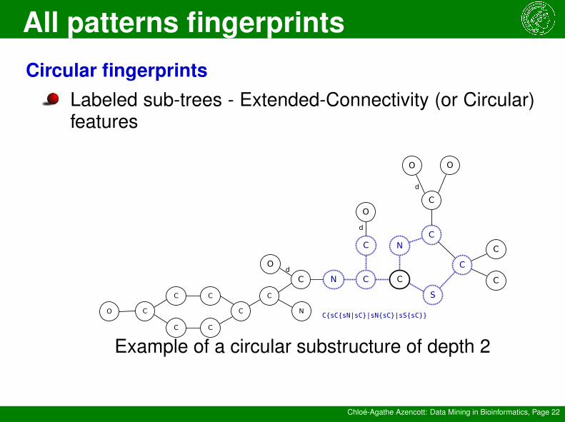
Circular fingerprintsLabeled sub-trees - Extended-Connectivity (or Circular)features
O
N C C
N
O
S
C
C
O O
C
Cd
d
d
C
C
C{sC{sN|sC}|sN{sC}|sS{sC}}
C
C
NC
C
C
C
C
CO
Example of a circular substructure of depth 2
All patterns fingerprints
Chloé-Agathe Azencott: Data Mining in Bioinformatics, Page 23
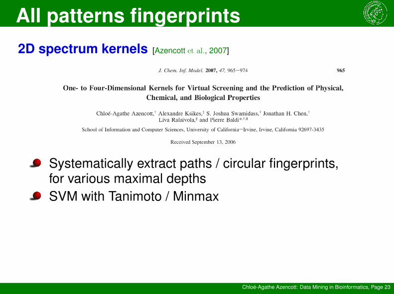
2D spectrum kernels [Azencott et al., 2007]
Systematically extract paths / circular fingerprints,for various maximal depthsSVM with Tanimoto / Minmax
All patterns fingerprints
Chloé-Agathe Azencott: Data Mining in Bioinformatics, Page 24
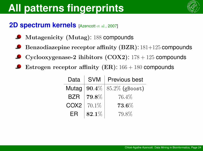
2D spectrum kernels [Azencott et al., 2007]
Mutagenicity (Mutag): 188 compounds
Benzodiazepine receptor affinity (BZR): 181+125 compounds
Cyclooxygenase-2 ihibitors (COX2): 178 + 125 compounds
Estrogen receptor affinity (ER): 166 + 180 compounds
Data SVM Previous bestMutag 90.4% 85.2% (gBoost)BZR 79.8% 76.4%
COX2 70.1% 73.6%
ER 82.1% 79.8%
Informative patterns
Chloé-Agathe Azencott: Data Mining in Bioinformatics, Page 25
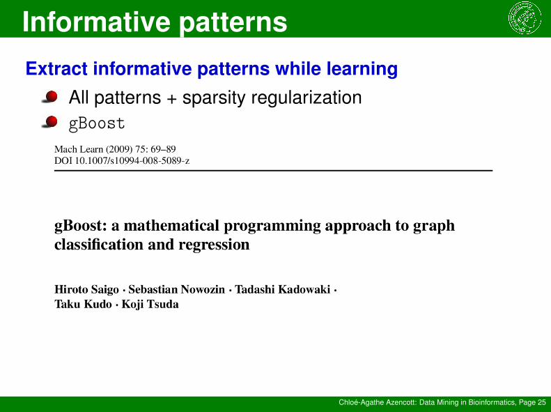
Extract informative patterns while learningAll patterns + sparsity regularizationgBoost
gBoost
Chloé-Agathe Azencott: Data Mining in Bioinformatics, Page 26
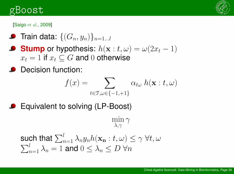
[Saigo et al., 2009]
Train data: {(Gn, yn)}n=1...l
Stump or hypothesis: h(x : t, ω) = ω(2xt − 1)xt = 1 if xt ⊆ G and 0 otherwise
Decision function:
f (x) =∑
t∈T,ω∈{−1,+1}
αtω h(x : t, ω)
Equivalent to solving (LP-Boost)
minλ,γ
γ
such that∑l
n=1 λnynh(xn : t, ω) ≤ γ ∀t, ω∑ln=1 λn = 1 and 0 ≤ λn ≤ D ∀n
gBoost
Chloé-Agathe Azencott: Data Mining in Bioinformatics, Page 27
[Saigo et al., 2009]
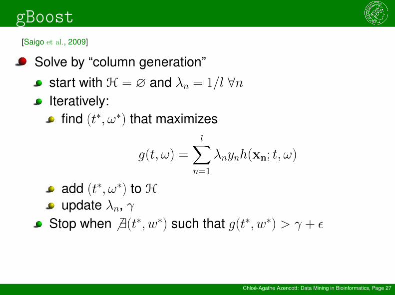
Solve by “column generation”
start with H = ∅ and λn = 1/l ∀nIteratively:
find (t∗, ω∗) that maximizes
g(t, ω) =l∑
n=1
λnynh(xn; t, ω)
add (t∗, ω∗) to H
update λn, γStop when 6 ∃(t∗, w∗) such that g(t∗, w∗) > γ + ε
gBoost
Chloé-Agathe Azencott: Data Mining in Bioinformatics, Page 28
[Saigo et al., 2009]
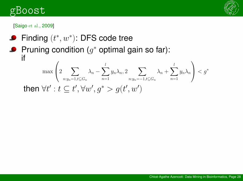
Finding (t∗, w∗): DFS code treePruning condition (g∗ optimal gain so far):if
max
2∑
n:yn=1,t⊆Gn
λn −l∑
n=1
ynλn, 2∑
n:yn=−1,t⊆Gn
λn +l∑
n=1
ynλn
< g∗
then ∀t′ : t ⊆ t′,∀w′, g∗ > g(t′, w′)
gBoost
Chloé-Agathe Azencott: Data Mining in Bioinformatics, Page 29
[Saigo et al., 2009]
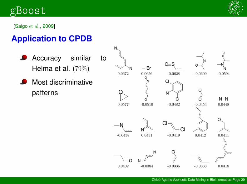
Application to CPDB
Accuracy similar toHelma et al. (79%)
Most discriminativepatterns
Weisfeiler-Lehman kernel
Chloé-Agathe Azencott: Data Mining in Bioinformatics, Page 30
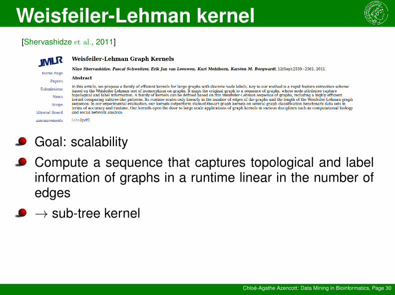
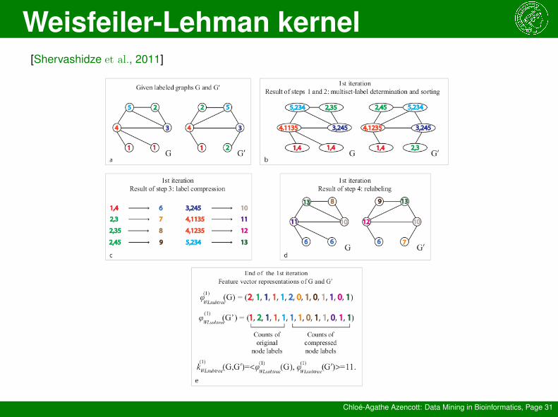
[Shervashidze et al., 2011]
Goal: scalability
Compute a sequence that captures topological and labelinformation of graphs in a runtime linear in the number ofedges
→ sub-tree kernel
Weisfeiler-Lehman kernel
Chloé-Agathe Azencott: Data Mining in Bioinformatics, Page 31
[Shervashidze et al., 2011]
Convolution kernels
Chloé-Agathe Azencott: Data Mining in Bioinformatics, Page 32
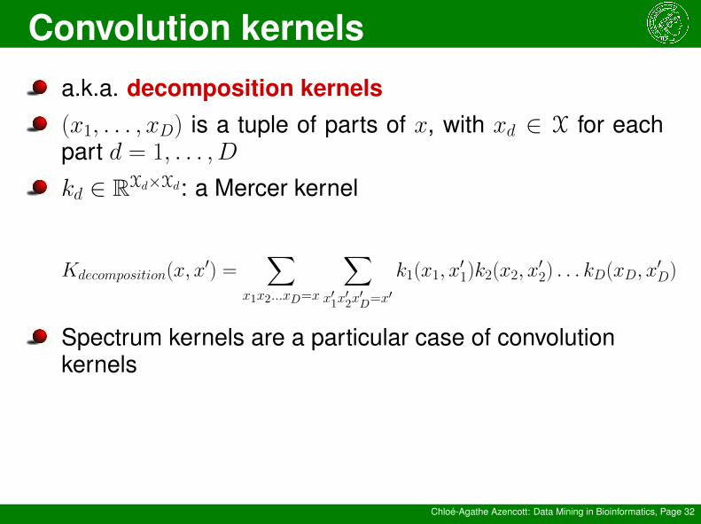
a.k.a. decomposition kernels(x1, . . . , xD) is a tuple of parts of x, with xd ∈ X for eachpart d = 1, . . . , D
kd ∈ RXd×Xd: a Mercer kernel
Kdecomposition(x, x′) =
∑x1x2...xD=x
∑x′1x′2x′D=x
′
k1(x1, x′1)k2(x2, x
′2) . . . kD(xD, x
′D)
Spectrum kernels are a particular case of convolutionkernels
Convolution kernels
Chloé-Agathe Azencott: Data Mining in Bioinformatics, Page 33
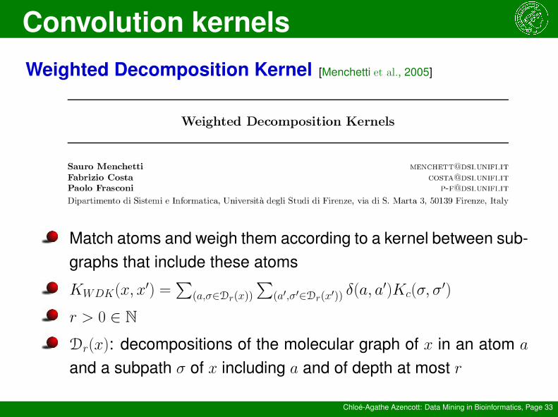
Weighted Decomposition Kernel [Menchetti et al., 2005]
Match atoms and weigh them according to a kernel between sub-graphs that include these atoms
KWDK(x, x′) =
∑(a,σ∈Dr(x))
∑(a′,σ′∈Dr(x′)) δ(a, a
′)Kc(σ, σ′)
r > 0 ∈ N
Dr(x): decompositions of the molecular graph of x in an atom a
and a subpath σ of x including a and of depth at most r
Convolution kernels
Chloé-Agathe Azencott: Data Mining in Bioinformatics, Page 34
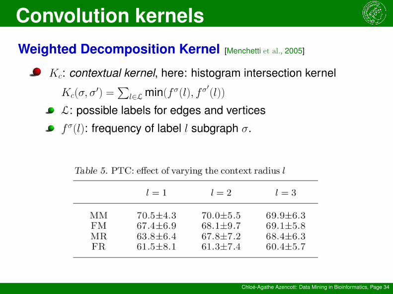
Weighted Decomposition Kernel [Menchetti et al., 2005]
Kc: contextual kernel, here: histogram intersection kernel
Kc(σ, σ′) =
∑l∈L min(fσ(l), fσ′(l))
L: possible labels for edges and vertices
fσ(l): frequency of label l subgraph σ.
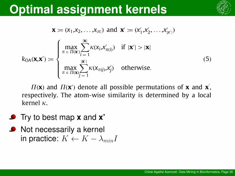
Optimal assignment kernels
Chloé-Agathe Azencott: Data Mining in Bioinformatics, Page 35
Try to best map x and x’Not necessarily a kernelin practice: K ← K − λminI
Optimal assignment kernels
Chloé-Agathe Azencott: Data Mining in Bioinformatics, Page 36
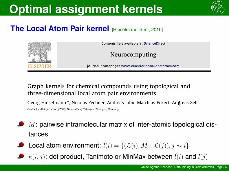
The Local Atom Pair kernel [Hinselmann et al., 2010]
M : pairwise intramolecular matrix of inter-atomic topological dis-tances
Local atom environment: l(i) = {(L(i),Mij,L(j)), j ∼ i}κ(i, j): dot product, Tanimoto or MinMax between l(i) and l(j)
Optimal assignment kernels
Chloé-Agathe Azencott: Data Mining in Bioinformatics, Page 37
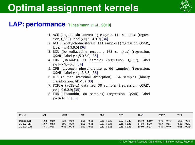
LAP: performance [Hinselmann et al., 2010]
Introducing spatial information
Chloé-Agathe Azencott: Data Mining in Bioinformatics, Page 38
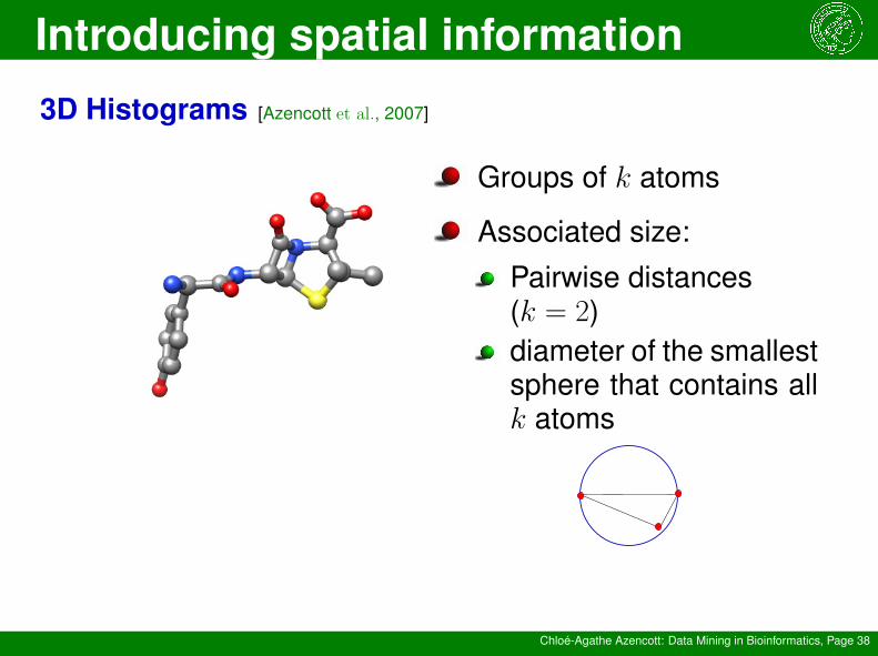
3D Histograms [Azencott et al., 2007]
Groups of k atoms
Associated size:
Pairwise distances(k = 2)diameter of the smallestsphere that contains allk atoms
Introducing spatial information
Chloé-Agathe Azencott: Data Mining in Bioinformatics, Page 39
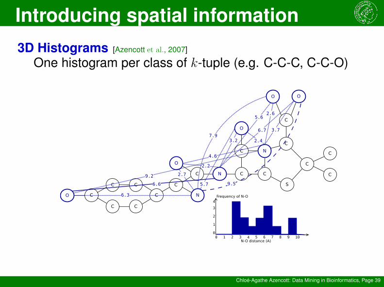
3D Histograms [Azencott et al., 2007]
One histogram per class of k-tuple (e.g. C-C-C, C-C-O)
C
O
N C
C
C
N
O
S
C
C
O O
C
C
C2.2
4.6
3.2
5.6
6.7
2.4
2.6
3.7
0 1 2 3 4 5 6 7
Frequency of N-O
N-O distance (A)
C
NC
C
C
C
C
CO 6.3
6.6
9.2 2.7
5.7
7.9
9.5
8 9 10
1
2
3
4
0
Introducing spatial information
Chloé-Agathe Azencott: Data Mining in Bioinformatics, Page 40
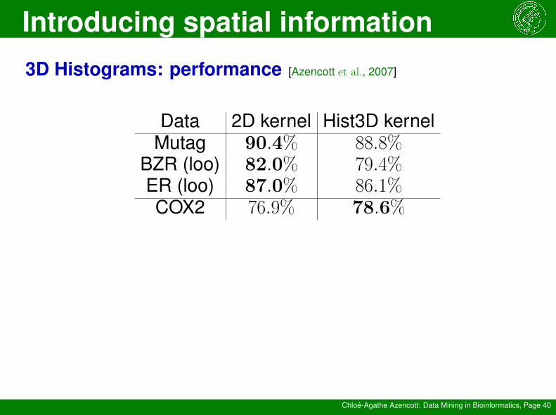
3D Histograms: performance [Azencott et al., 2007]
Data 2D kernel Hist3D kernelMutag 90.4% 88.8%
BZR (loo) 82.0% 79.4%ER (loo) 87.0% 86.1%COX2 76.9% 78.6%
Introducing spatial information
Chloé-Agathe Azencott: Data Mining in Bioinformatics, Page 41
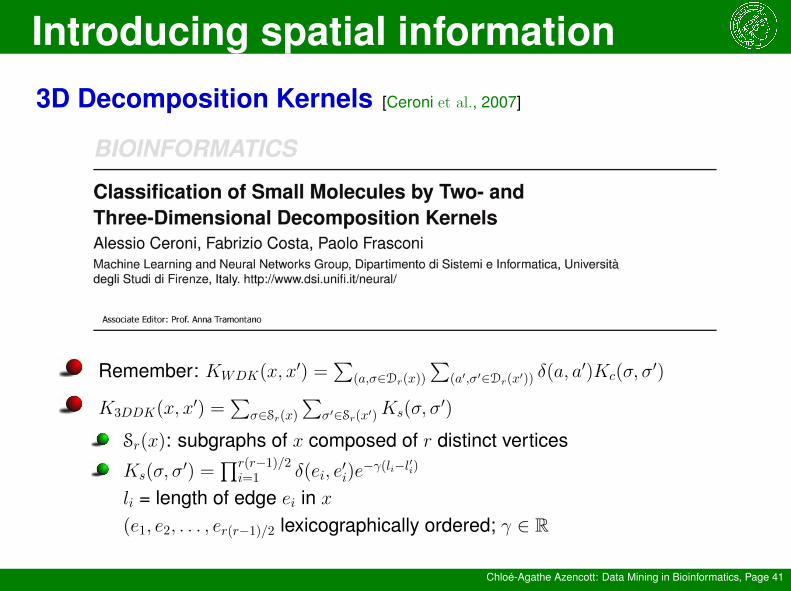
3D Decomposition Kernels [Ceroni et al., 2007]
Remember: KWDK(x, x′) =
∑(a,σ∈Dr(x))
∑(a′,σ′∈Dr(x′))
δ(a, a′)Kc(σ, σ′)
K3DDK(x, x′) =
∑σ∈Sr(x)
∑σ′∈Sr(x′)Ks(σ, σ
′)
Sr(x): subgraphs of x composed of r distinct vertices
Ks(σ, σ′) =
∏r(r−1)/2i=1 δ(ei, e
′i)e−γ(li−l′i)
li = length of edge ei in x(e1, e2, . . . , er(r−1)/2 lexicographically ordered; γ ∈ R
Introducing spatial information
Chloé-Agathe Azencott: Data Mining in Bioinformatics, Page 42
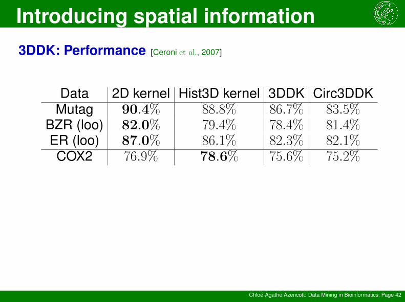
3DDK: Performance [Ceroni et al., 2007]
Data 2D kernel Hist3D kernel 3DDK Circ3DDKMutag 90.4% 88.8% 86.7% 83.5%
BZR (loo) 82.0% 79.4% 78.4% 81.4%ER (loo) 87.0% 86.1% 82.3% 82.1%COX2 76.9% 78.6% 75.6% 75.2%
Introducing spatial information
Chloé-Agathe Azencott: Data Mining in Bioinformatics, Page 43
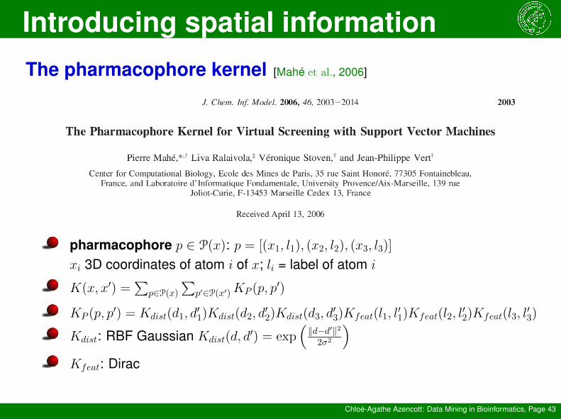
The pharmacophore kernel [Mahé et al., 2006]
pharmacophore p ∈ P(x): p = [(x1, l1), (x2, l2), (x3, l3)]
xi 3D coordinates of atom i of x; li = label of atom i
K(x, x′) =∑
p∈P(x)∑
p′∈P(x′)KP (p, p′)
KP (p, p′) = Kdist(d1, d
′1)Kdist(d2, d
′2)Kdist(d3, d
′3)Kfeat(l1, l
′1)Kfeat(l2, l
′2)Kfeat(l3, l
′3)
Kdist: RBF Gaussian Kdist(d, d′) = exp
(‖d−d′‖22σ2
)Kfeat: Dirac
Introducing spatial information
Chloé-Agathe Azencott: Data Mining in Bioinformatics, Page 44
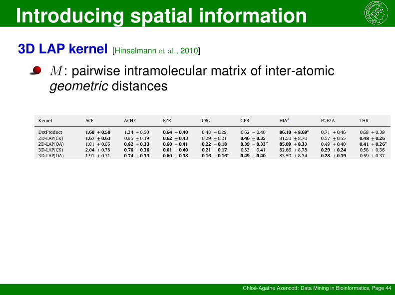
3D LAP kernel [Hinselmann et al., 2010]
M : pairwise intramolecular matrix of inter-atomicgeometric distances
Introducing spatial information
Chloé-Agathe Azencott: Data Mining in Bioinformatics, Page 45
ConclusionHow relevant is 3D information?How good is 3D information?
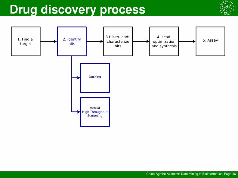
Drug discovery process
Chloé-Agathe Azencott: Data Mining in Bioinformatics, Page 46
Docking
VirtualHigh-Throughput
Screening
1. Find a target
2. Identifyhits
3.Hit-to-lead: characterize
hits
4. Lead optimization
and synthesis
5. Assay
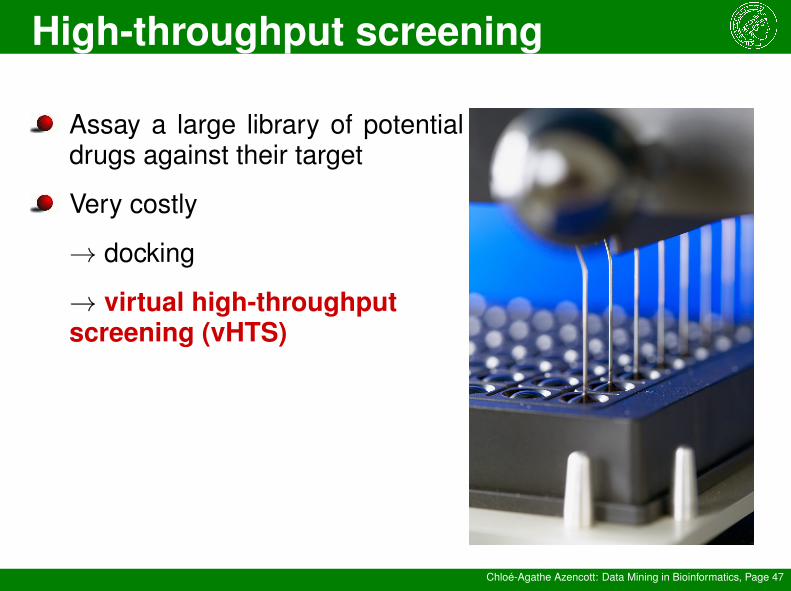
High-throughput screening
Chloé-Agathe Azencott: Data Mining in Bioinformatics, Page 47
Assay a large library of potentialdrugs against their target
Very costly
→ docking
→ virtual high-throughputscreening (vHTS)
Measuring performance
Chloé-Agathe Azencott: Data Mining in Bioinformatics, Page 48
Imbalanced data
Typically, most compounds are inactive ⇒ many more negativethan positive examples
E.g. DHFR data set:99, 995 chemicals screened for activity against dihydrofolatereductase; < 0.2% active compounds
Accuracy is not appropriate:predicting all compounds negative⇒ accuracy = 99.8%
sensitivity= # True Positives# Positives
specificity= # True Negatives# Negatives
For many methods, the output is continuous⇒ accuracy, sensitivity and specificity depend on a threshold θ
Measuring performance
Chloé-Agathe Azencott: Data Mining in Bioinformatics, Page 49
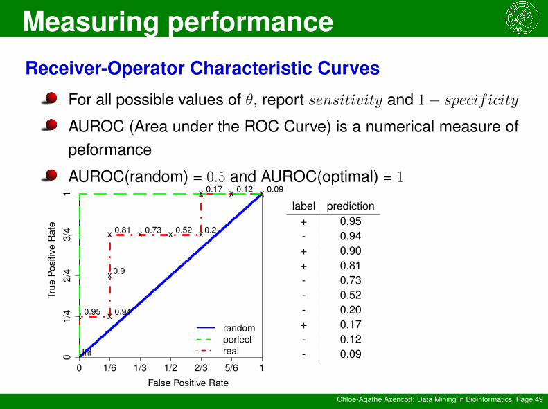
Receiver-Operator Characteristic Curves
For all possible values of θ, report sensitivity and 1− specificityAUROC (Area under the ROC Curve) is a numerical measure ofpeformance
AUROC(random) = 0.5 and AUROC(optimal) = 1
0 1/6 1/3 1/2 2/3 5/6 1
01
/42
/43
/41
False Positive Rate
Tru
e P
ositiv
e R
ate
x
x x
x
x x x x
x x x
Inf
0.95 0.94
0.9
0.81 0.73 0.52 0.2
0.17 0.12 0.09
random
perfect
real
label prediction+ 0.95- 0.94+ 0.90+ 0.81- 0.73- 0.52- 0.20+ 0.17- 0.12- 0.09
Measuring performance
Chloé-Agathe Azencott: Data Mining in Bioinformatics, Page 50
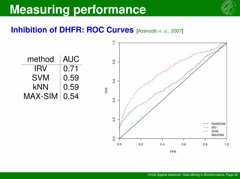
Inhibition of DHFR: ROC Curves [Azencott et al., 2007]
method AUCIRV 0.71SVM 0.59kNN 0.59
MAX-SIM 0.54
0.0 0.2 0.4 0.6 0.8 1.0
0.0
0.2
0.4
0.6
0.8
1.0
FPR
TP
R
RANDOM
IRV
SVM
MAXSIM
Measuring performance
Chloé-Agathe Azencott: Data Mining in Bioinformatics, Page 51
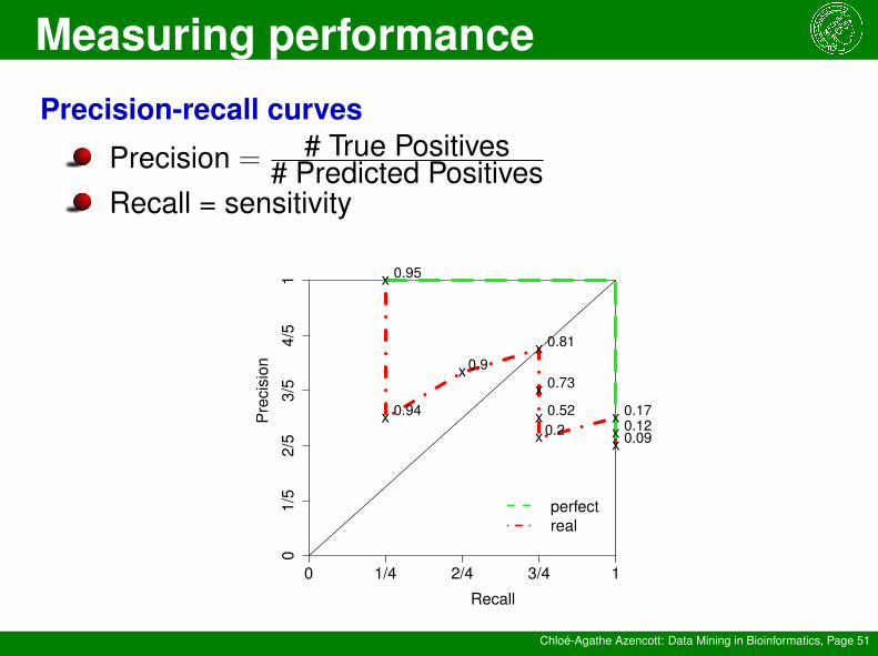
Precision-recall curves
Precision = # True Positives# Predicted Positives
Recall = sensitivity
0 1/4 2/4 3/4 1
01/5
2/5
3/5
4/5
1
Recall
Pre
cis
ion
x
x
x
x
x
x
x
xxx
0.95
0.94
0.9
0.81
0.73
0.52
0.2
0.170.120.09
perfect
real
Other applications
Chloé-Agathe Azencott: Data Mining in Bioinformatics, Page 52
Other applications of graph mining in chemoinformatics
Database indexing and searchPrediction of 3D structures of small compoundsand proteinsReaction Prediction
References and further reading
Chloé-Agathe Azencott: Data Mining in Bioinformatics, Page 53
[Azencott et al., 2007] Azencott, C.-A., Ksikes, A., Swamidass, S. J., Chen, J. H., Ralaivola, L. and Baldi, P. (2007). One-to four-dimensional kernels for virtual screening and the prediction of physical, chemical, and biological properties. Journal of chemical
information and modeling 47, 965–974. 23, 24, 38, 39, 40, 50
[Baldi et al., 2007] Baldi, P., Benz, R. W., Hirschberg, D. S. and Swamidass, S. J. (2007). Lossless compression of chemical fingerprintsusing integer entropy codes improves storage and retrieval. Journal of chemical information and modeling 47, 2098–2109. 16
[Ceroni et al., 2007] Ceroni, A., Costa, F. and Frasconi, P. (2007). Classification of small molecules by two-and three-dimensionaldecomposition kernels. Bioinformatics 23, 2038–2045. 41, 42
[Helma et al., 2004] Helma, C., Cramer, T., Kramer, S. and De Raedt, L. (2004). Data mining and machine learning techniques forthe identification of mutagenicity inducing substructures and structure activity relationships of noncongeneric compounds. Journal ofchemical information and computer sciences 44, 1402–1411. 17, 18
[Hinselmann et al., 2010] Hinselmann, G., Fechner, N., Jahn, A., Eckert, M. and Zell, A. (2010). Graph kernels for chemical compoundsusing topological and three-dimensional local atom pair environments. Neurocomputing 74, 219–229. 36, 37, 44
[Mahé et al., 2006] Mahé, P., Ralaivola, L., Stoven, V. and Vert, J.-P. (2006). The pharmacophore kernel for virtual screening withsupport vector machines. Journal of chemical information and modeling 46, 2003–2014. 43
[Menchetti et al., 2005] Menchetti, S., Costa, F. and Frasconi, P. (2005). Weighted Decomposition Kernels. In Proceedings of the 22nd
International Conference on Machine Learning pp. 585–592, ACM, Bonn, Germany. 33, 34
[Saigo et al., 2009] Saigo, H., Nowozin, S., Kadowaki, T., Kudo, T. and Tsuda, K. (2009). gBoost: a mathematical programmingapproach to graph classification and regression. Machine Learning 75, 69–89. 26, 27, 28, 29
[Shervashidze et al., 2011] Shervashidze, N., Schweitzer, P., van Leeuwen, E. J., Mehlhorn, K. and Borgwardt, K. M. (2011). Weisfeiler-Lehman graph kernels. Journal of Machine Learning Research 12, 2539–2561. 30, 31

The end
Chloé-Agathe Azencott: Data Mining in Bioinformatics, Page 54
Tomorrow: Projects Presentations
By 9:45 AM on Friday, March 1, 2013, please submit the following byemail to Prof. Borgwardt:
A short report on your project, that gives your answers to the ques-tions in Section 2 (You can ignore Section 1 here) in your exercisesheet
The code that you wrote as part of your project
Your presentation slides as a PDF.


![Data Mining in Bioinformatics Day 8: Clustering in ......Hierarchical clustering Karsten Borgwardt: Data Mining in Bioinformatics, Page 24 [Eisen et al., 1998] cluster E: genes encoding](https://img.pdfslide.us/doc/110x75/5f0d133d7e708231d4388e3e/data-mining-in-bioinformatics-day-8-clustering-in-hierarchical-clustering.jpg)