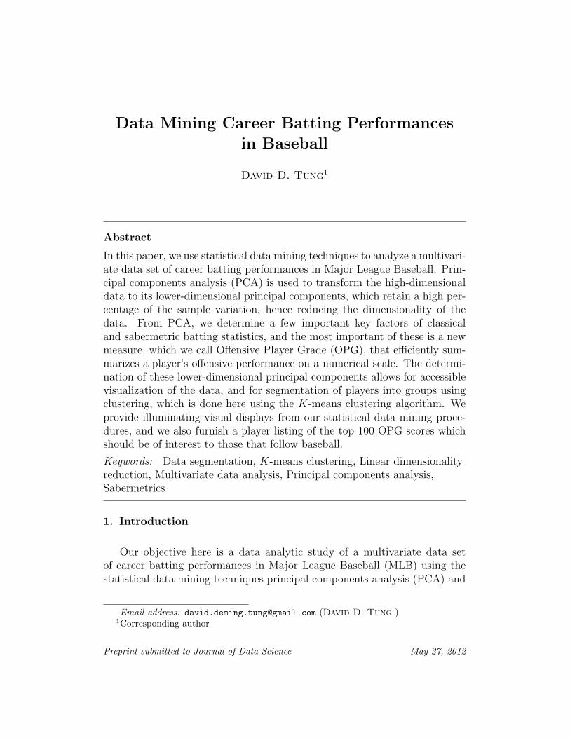
Data Mining Career Batting Performances

in Baseball

David D. Tung1

Abstract

In this paper, we use statistical data mining techniques to analyze a multivari-ate data set of career batting performances in Major League Baseball. Prin-cipal components analysis (PCA) is used to transform the high-dimensionaldata to its lower-dimensional principal components, which retain a high per-centage of the sample variation, hence reducing the dimensionality of thedata. From PCA, we determine a few important key factors of classicaland sabermetric batting statistics, and the most important of these is a newmeasure, which we call Offensive Player Grade (OPG), that efficiently sum-marizes a player’s offensive performance on a numerical scale. The determi-nation of these lower-dimensional principal components allows for accessiblevisualization of the data, and for segmentation of players into groups usingclustering, which is done here using the K-means clustering algorithm. Weprovide illuminating visual displays from our statistical data mining proce-dures, and we also furnish a player listing of the top 100 OPG scores whichshould be of interest to those that follow baseball.

Keywords: Data segmentation, K-means clustering, Linear dimensionalityreduction, Multivariate data analysis, Principal components analysis,Sabermetrics

1. Introduction

Our objective here is a data analytic study of a multivariate data setof career batting performances in Major League Baseball (MLB) using thestatistical data mining techniques principal components analysis (PCA) and

Email address: david.deming.tung@gmail.com (David D. Tung )1Corresponding author

Preprint submitted to Journal of Data Science May 27, 2012

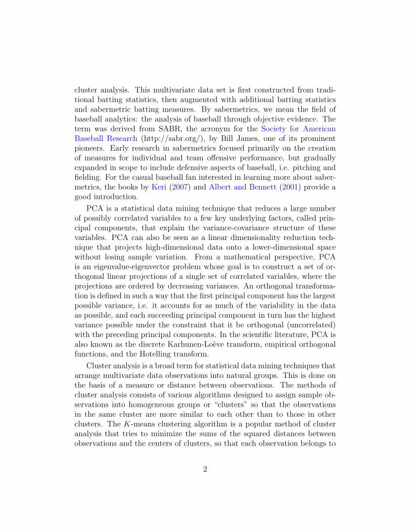
cluster analysis. This multivariate data set is first constructed from tradi-tional batting statistics, then augmented with additional batting statisticsand sabermetric batting measures. By sabermetrics, we mean the field ofbaseball analytics: the analysis of baseball through objective evidence. Theterm was derived from SABR, the acronym for the Society for AmericanBaseball Research (http://sabr.org/), by Bill James, one of its prominentpioneers. Early research in sabermetrics focused primarily on the creationof measures for individual and team offensive performance, but graduallyexpanded in scope to include defensive aspects of baseball, i.e. pitching andfielding. For the casual baseball fan interested in learning more about saber-metrics, the books by Keri (2007) and Albert and Bennett (2001) provide agood introduction.

PCA is a statistical data mining technique that reduces a large numberof possibly correlated variables to a few key underlying factors, called prin-cipal components, that explain the variance-covariance structure of thesevariables. PCA can also be seen as a linear dimensionality reduction tech-nique that projects high-dimensional data onto a lower-dimensional spacewithout losing sample variation. From a mathematical perspective, PCAis an eigenvalue-eigenvector problem whose goal is to construct a set of or-thogonal linear projections of a single set of correlated variables, where theprojections are ordered by decreasing variances. An orthogonal transforma-tion is defined in such a way that the first principal component has the largestpossible variance, i.e. it accounts for as much of the variability in the dataas possible, and each succeeding principal component in turn has the highestvariance possible under the constraint that it be orthogonal (uncorrelated)with the preceding principal components. In the scientific literature, PCA isalso known as the discrete Karhunen-Loeve transform, empirical orthogonalfunctions, and the Hotelling transform.

Cluster analysis is a broad term for statistical data mining techniques thatarrange multivariate data observations into natural groups. This is done onthe basis of a measure or distance between observations. The methods ofcluster analysis consists of various algorithms designed to assign sample ob-servations into homogeneous groups or “clusters” so that the observationsin the same cluster are more similar to each other than to those in otherclusters. The K-means clustering algorithm is a popular method of clusteranalysis that tries to minimize the sums of the squared distances betweenobservations and the centers of clusters, so that each observation belongs to

2

the cluster with the nearest mean. This results in a partitioning of the datainto Voronoi cells. Clustering is the most well-known example of unsuper-vised learning, and is philosophically different from classification, which likeregression is a supervised learning technique. In classification, it is knownhow many classes or groups are present in the data and which observationsare members of which class or group. The objective of classification is toclassify new observations into one of the known classes based on a learningset of the data. In clustering, the number of classes is unknown and so is themembership of observations into classes. Clustering is also known as datasegmentation and is used in many fields, including market research, biology,machine learning, pattern recognition, image analysis, information retrieval,and bioinformatics.

For a more thorough introduction to PCA and cluster analysis, as well asstatistical data mining, the reader is referred to Tuffery (2011), Johnson andWichern (2007), Hastie et al. (2009), and Izenman (2008). Wu et al. (2008)surveys the top data mining algorithms, covering classification, clustering,statistical learning, association analysis, and link mining. Jain (2010) surveysresearch done on cluster analysis. Bock (2008) presents a historical viewof the K-means clustering algorithm. Biau et al. (2008) discusses K-meansclustering when sample observations take values in a separable Hilbert space.Melnykov and Maitra (2010) surveys model-based clustering based on finitemixture models.

Data preparation and data description is detailed in the next section.PCA and K-means clustering is seen in Section 3. In Section 4, we discussthe PCA derived measure Offensive Player Grade (OPG).

2. Data Preparation and Description

A multivariate data set of career batting performances for MLB playerswas constructed from standard batting data found in the Lahman baseballdatabase, available on the internet at http://baseball1.com/statistics. Ver-sion 5.9 of the database was used, which covers all seasons through the year2011. The players’ surnames and first names and ID code were queriedfrom the ‘Master’ table of the database. Then player data for the followingbatting statistics were extracted from the ‘Batting’ table of the database:Games (G), At Bats (AB), Runs (R), Hits (H), Doubles (2B), Triples (3B),Home Runs (HR), Runs Batted In (RBI), Stolen Bases (SB), Caught Stealing

3

(CS), Walks (BB), Strikeouts (K), Intentional Walks (IBB), Hit By Pitcher(HBP), Sacrifice Hits (SH), Sacrifice Flies (SF), and Ground Into DoublePlay (GIDP). These batting statistics are frequencies or counts, and are thebasic building blocks for more complicated batting measures. Several of thesebatting statistics have incomplete data observations: SF is complete from theyear 1954 on, CS is complete from the year 1951 on, SH is complete from theyear 1894 on, HBP is complete from the year 1887 on, SB is complete fromthe year 1886 on. Where data was unavailable, its value was assumed to bezero following standard convention.

After transferring the extracted data to a spreadsheet, the following clas-sical and sabermetric batting statistics were also calculated for inclusion intothe data set: Total Bases (TB), Batting Average (BA), On Base Percentage(OBP), Slugging Average (SLG), On Base Plus Slugging (OPS), Total Aver-age (TA), Isolated Power (ISO), Secondary Average (SECA), Runs Created(RC), and Runs Created per Game (RC27). Formulae are given below:

TB = H + 2B + 2(3B) + 3(HR), (2.1)

BA =H

AB, (2.2)

OBP =H + BB + HBP

AB + BB + HBP + SF, (2.3)

SLG =TB

AB, (2.4)

OPS = OBP + SLG, (2.5)

TA =TB + BB + HBP + SB − CS

AB − H + CS + GIDP, (2.6)

ISO = SLG− BA =TB− H

AB, (2.7)

SECA =TB − H + BB + SB − CS

AB, (2.8)

RC =

(H + BB + HBP − CS − GIDP)· [ TB + 0.26(BB − IBB + HBP) + 0.52(SH + SF + SB)]

AB + BB + HBP + SH + SF,

(2.9)

RC27 =RC

(AB − H + SH + SF + CS + GIDP)/27. (2.10)

For completeness, we will briefly summarize these batting statistics. Total

4

Bases (TB) is the number of bases a player has gained with hits, i.e. the sumof his hits weighted by 1 for a single, 2 for a double, 3 for a triple and 4 fora home run. Batting Average (BA) is the most famous and quoted of allbaseball statistics: it is the ratio of hits to at-bats, not counting walks, hitby pitcher, or sacrifices. On Base Percentage (OBP) is the classical measurefor judging how good a batter is at getting on base: total number of timeson base divided by the total of at-bats, walks, hit by pitcher, and sacrificeflies. Slugging Average (SLG) is the classical measure of a batter’s powerhitting ability: total bases on hits divided by at-bats. The classic trio ofbatting statistics (BA, OBP, SLG) presented together, provide an excellentsummary of a player’s offensive ability, combining the ability to get on baseand to hit for power. For example, a player with (BA = 0.300, OBP = 0.400,SLG = 0.500) is considered an ideal offensive player.

The statistics we describe below are modern sabermetric batting mea-sures. The ability of a player to both get on base and to hit for power, twoimportant hitting skills, are represented in the famous sabermetric measureOn Base Plus Slugging (OPS), which is obtained by simply adding OBPand SLG. OPS is a quick and dirty statistic that correlates better with runsscoring than BA, OBP, or SLG alone. Total Average (TA) is essentially amodification of SLG, and is rather similar to OPS. Isolated Power (ISO) isa measure used to evaluate a batter’s pure power hitting ability. Since OBPand SLG are highly correlated, ISO was designed as an alternative measureof a player’s ability to hit for power not confounded with his ability to geton base. Secondary Average (SECA) is a modification of ISO and TA, anda good measure of extra base ability: the ratio of bases gained from othersources (extra base hits, walks and net stolen bases) to at-bats. Runs Cre-ated (RC) was created by Bill James and estimates the number of runs aplayers contributes to his team. Since RC estimates total run production,Runs Created per Game (RC27) is the conversion of RC to a rate statistic:RC is divided by an estimate of the number of games a player’s offensiverecord represents. This is done by estimating the total number of outs anddividing by 27 (27 outs in a 9 inning baseball game). RC27 estimates thenumber of runs produced by a team composed solely of the player analyzed.

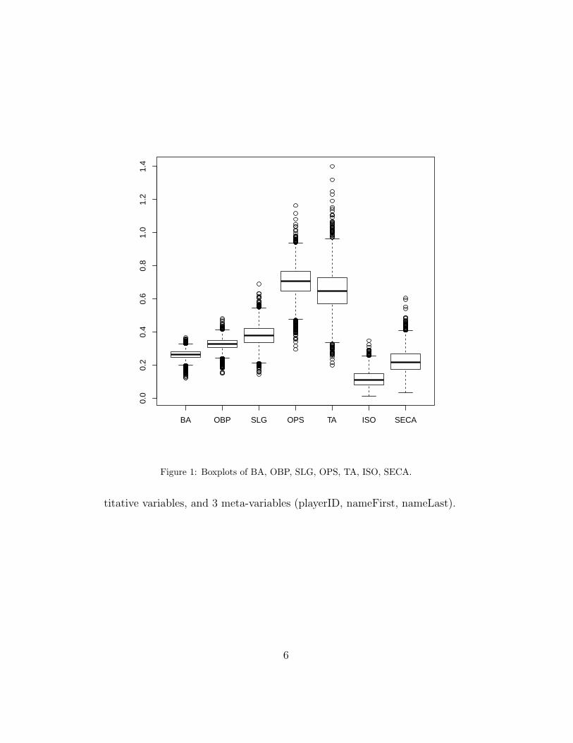
Only players with at least 1000 at-bats were considered in order to createa diverse collection of players for the data set, e.g. pitchers with significantbatting experience, lesser known “rank and file” type players, and activeplayers. The fully constructed data set contains 3491 observations, 27 quan-

5

BA OBP SLG OPS TA ISO SECA

0.0

0.2

0.4

0.6

0.8

1.0

1.2

1.4

Figure 1: Boxplots of BA, OBP, SLG, OPS, TA, ISO, SECA.

titative variables, and 3 meta-variables (playerID, nameFirst, nameLast).

6

24

68

1012

14

RC27

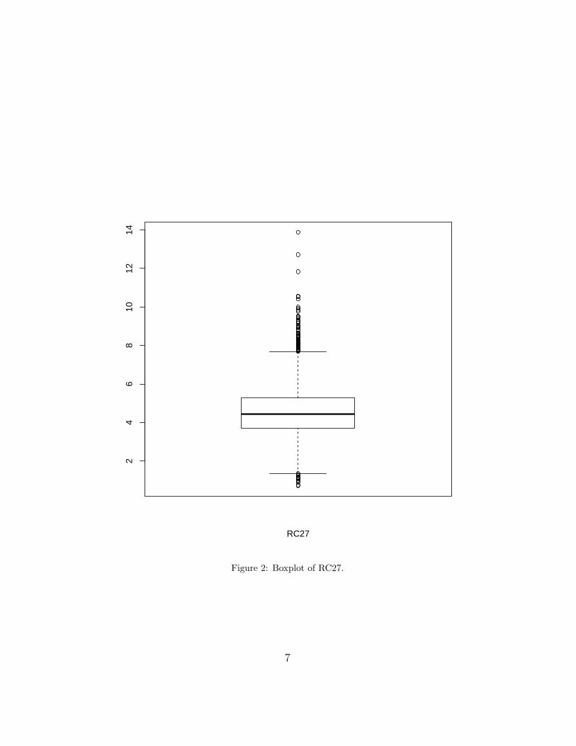
Figure 2: Boxplot of RC27.

7

3. Dimensionality Reduction and Clustering viaPrincipal Components Analysis

In this section, we analyze the batting statistics (BA, OBP, SLG, OPS,TA, ISO, SECA, RC27) through PCA and clustering. For this purpose, wetake the 3491 observations and these 8 variables or features as our workingdata set. Our data set can be represented by a data matrix X with n rowsand p columns, where the rows represent the observations as p-dimensionalvectors, and the columns represent the variables:

X =

xT1

xT2...xTn

=

x11 x12 . . . x1p

x21 x22 . . . x2p...

.... . .

...xn1 xn2 . . . xnp

. (3.1)

Here n = 3491 and p = 8. Visualizing 3491 points in an 8-dimensionalspace is rather troublesome, since we are used to visualizing at most three-dimensional data. PCA is a standard technique used to reduce a large numberof dimensions down to two or three dimensions for accessible visualization.The principal components are the new set of dimensions, where the firstdimension is the one that retains most of the original data’s variance.

We first introduce some extra notation from linear algebra and multivari-ate analysis. The n × 1 column vector whose entries are all 1 is denotedby

1 =

11...1

. (3.2)

The n× n matrix whose entries are all 1 is denoted by

11T =

1 1 . . . 11 1 . . . 1...

.... . .

...1 1 . . . 1

. (3.3)

8

The p× 1 vector of column means from the data matrix X can be written as

x =

x1

x2...xp

=1

nXT1. (3.4)

The n× p matrix of column means is denoted by

1

n11TX =

x1 x2 . . . xp

x1 x2 . . . xp...

.... . .

...x1 x2 . . . xp

. (3.5)

The sample variance-covariance matrix for the data matrix X is a p × pmatrix defined by

SX =1

n− 1

(X− 1

n11TX

)T (X− 1

n11TX

)=

1

n− 1XT

(I− 1

n11T

)X,

(3.6)where I is the n × n identity matrix whose entries are zero except on thediagonal where they are all 1.

In practice, variables measured on different scales or on a common scalewith differing ranges are typically standardized by constructing the standard-ized observations

zi = D−1/2(xi − x) =

xi1−x1√

s11xi2−x2√

s22...

xip−xp√spp

, i = 1, 2, . . . , n, (3.7)

where

D1/2 =

√s11 0 . . . 00

√s22 . . . 0

......

. . ....

0 0 . . .√spp

, (3.8)

9

is the sample standard deviation matrix. We will use

Z =

zT1zT2...zTn

=

x11−x1√

s11

x12−x2√s22

. . .x1p−xp√

sppx21−x1√

s11

x22−x2√s22

. . .x2p−xp√

spp...

.... . .

...xn1−x1√

s11

xn2−x2√s22

. . . xnp−xp√spp

=

(X− 1

n11TX

)D−1/2,

(3.9)to denote the standardized data matrix.

Observe that the sample variance-covariance matrix of Z is the samplecorrelation matrix of X, i.e.

SZ =1

n− 1

(Z− 1

n11TZ

)T (Z− 1

n11TZ

)=

1

n− 1ZTZ = D−1/2SXD

−1/2

= R. (3.10)

Since R is a symmetric matrix, it has the eigendecomposition

R = QΛQT , (3.11)

where Q is a p×p orthogonal matrix whose columns are the unit eigenvectorsof R, and Λ = diag(λ1, λ2, . . . , λp) is a diagonal matrix whose entries arethe eigenvalues of R, which are arranged in decreasing order. Note thatQT = Q−1.

The sample principal components are obtained by an orthogonal trans-formation of the standardized data matrix, i.e.

Z 7→ Y = ZQ, (3.12)

whereQ is the orthogonal matrix from the eigendecomposition. Equivalently,the sample principal components can be obtained from the original datamatrix X by the transformation:

X 7→ Y =

(X− 1

n11TX

)D−1/2Q. (3.13)

The sample variance-covariance matrix of Y = ZQ is given by Λ, the

10

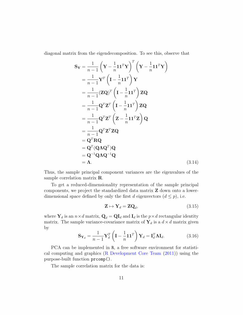
diagonal matrix from the eigendecomposition. To see this, observe that

SY =1

n− 1

(Y− 1

n11TY

)T (Y− 1

n11TY

)=

1

n− 1YT

(I− 1

n11T

)Y

=1

n− 1(ZQ)T

(I− 1

n11T

)ZQ

=1

n− 1QTZT

(I− 1

n11T

)ZQ

=1

n− 1QTZT

(Z− 1

n11TZ

)Q

=1

n− 1QTZTZQ

= QTRQ

= QT (QΛQT )Q

= Q−1QΛQ−1Q

= Λ. (3.14)

Thus, the sample principal component variances are the eigenvalues of thesample correlation matrix R.

To get a reduced-dimensionality representation of the sample principalcomponents, we project the standardized data matrix Z down onto a lower-dimensional space defined by only the first d eigenvectors (d ≤ p), i.e.

Z 7→ Yd = ZQd, (3.15)

whereYd is an n×d matrix, Qd = QId and Id is the p×d rectangular identitymatrix. The sample variance-covariance matrix of Yd is a d×d matrix givenby

SYd=

1

n− 1YT

d

(I− 1

n11T

)Yd = ITdΛId. (3.16)

PCA can be implemented in R, a free software environment for statisti-cal computing and graphics (R Development Core Team (2011)) using thepurpose-built function prcomp().

The sample correlation matrix for the data is:

11

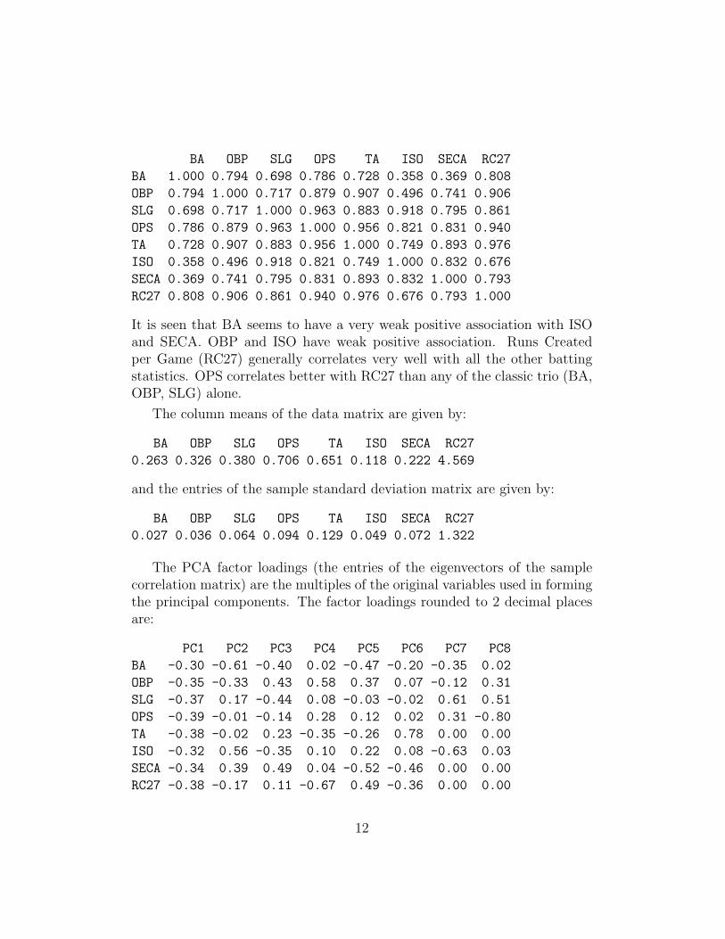
BA OBP SLG OPS TA ISO SECA RC27

BA 1.000 0.794 0.698 0.786 0.728 0.358 0.369 0.808

OBP 0.794 1.000 0.717 0.879 0.907 0.496 0.741 0.906

SLG 0.698 0.717 1.000 0.963 0.883 0.918 0.795 0.861

OPS 0.786 0.879 0.963 1.000 0.956 0.821 0.831 0.940

TA 0.728 0.907 0.883 0.956 1.000 0.749 0.893 0.976

ISO 0.358 0.496 0.918 0.821 0.749 1.000 0.832 0.676

SECA 0.369 0.741 0.795 0.831 0.893 0.832 1.000 0.793

RC27 0.808 0.906 0.861 0.940 0.976 0.676 0.793 1.000

It is seen that BA seems to have a very weak positive association with ISOand SECA. OBP and ISO have weak positive association. Runs Createdper Game (RC27) generally correlates very well with all the other battingstatistics. OPS correlates better with RC27 than any of the classic trio (BA,OBP, SLG) alone.

The column means of the data matrix are given by:

BA OBP SLG OPS TA ISO SECA RC27

0.263 0.326 0.380 0.706 0.651 0.118 0.222 4.569

and the entries of the sample standard deviation matrix are given by:

BA OBP SLG OPS TA ISO SECA RC27

0.027 0.036 0.064 0.094 0.129 0.049 0.072 1.322

The PCA factor loadings (the entries of the eigenvectors of the samplecorrelation matrix) are the multiples of the original variables used in formingthe principal components. The factor loadings rounded to 2 decimal placesare:

PC1 PC2 PC3 PC4 PC5 PC6 PC7 PC8

BA -0.30 -0.61 -0.40 0.02 -0.47 -0.20 -0.35 0.02

OBP -0.35 -0.33 0.43 0.58 0.37 0.07 -0.12 0.31

SLG -0.37 0.17 -0.44 0.08 -0.03 -0.02 0.61 0.51

OPS -0.39 -0.01 -0.14 0.28 0.12 0.02 0.31 -0.80

TA -0.38 -0.02 0.23 -0.35 -0.26 0.78 0.00 0.00

ISO -0.32 0.56 -0.35 0.10 0.22 0.08 -0.63 0.03

SECA -0.34 0.39 0.49 0.04 -0.52 -0.46 0.00 0.00

RC27 -0.38 -0.17 0.11 -0.67 0.49 -0.36 0.00 0.00

12

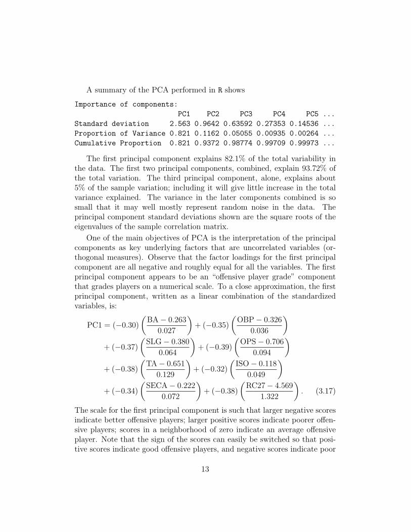
A summary of the PCA performed in R shows

Importance of components:

PC1 PC2 PC3 PC4 PC5 ...

Standard deviation 2.563 0.9642 0.63592 0.27353 0.14536 ...

Proportion of Variance 0.821 0.1162 0.05055 0.00935 0.00264 ...

Cumulative Proportion 0.821 0.9372 0.98774 0.99709 0.99973 ...

The first principal component explains 82.1% of the total variability inthe data. The first two principal components, combined, explain 93.72% ofthe total variation. The third principal component, alone, explains about5% of the sample variation; including it will give little increase in the totalvariance explained. The variance in the later components combined is sosmall that it may well mostly represent random noise in the data. Theprincipal component standard deviations shown are the square roots of theeigenvalues of the sample correlation matrix.

One of the main objectives of PCA is the interpretation of the principalcomponents as key underlying factors that are uncorrelated variables (or-thogonal measures). Observe that the factor loadings for the first principalcomponent are all negative and roughly equal for all the variables. The firstprincipal component appears to be an “offensive player grade” componentthat grades players on a numerical scale. To a close approximation, the firstprincipal component, written as a linear combination of the standardizedvariables, is:

PC1 = (−0.30)

(BA− 0.263

0.027

)+ (−0.35)

(OBP− 0.326

0.036

)+ (−0.37)

(SLG− 0.380

0.064

)+ (−0.39)

(OPS− 0.706

0.094

)+ (−0.38)

(TA− 0.651

0.129

)+ (−0.32)

(ISO− 0.118

0.049

)+ (−0.34)

(SECA− 0.222

0.072

)+ (−0.38)

(RC27− 4.569

1.322

). (3.17)

The scale for the first principal component is such that larger negative scoresindicate better offensive players; larger positive scores indicate poorer offen-sive players; scores in a neighborhood of zero indicate an average offensiveplayer. Note that the sign of the scores can easily be switched so that posi-tive scores indicate good offensive players, and negative scores indicate poor

13

offensive players: the negative signs are just an inconsequential artifact fromthe PCA numerical computations. Here and throughout, we define OPG =−PC1 to be the Offensive Player Grade statistic, and use the formula

OPG = 0.30

(BA− 0.263

0.027

)+ 0.35

(OBP− 0.326

0.036

)+ 0.37

(SLG− 0.380

0.064

)+ 0.39

(OPS− 0.706

0.094

)+ 0.38

(TA− 0.651

0.129

)+ 0.32

(ISO− 0.118

0.049

)+ 0.34

(SECA− 0.222

0.072

)+ 0.38

(RC27− 4.569

1.322

). (3.18)

In the next section, we will see that the OPG statistic is useful for summa-rizing a batter’s overall offensive performance with just one single number.

The factor loadings for the second principal component indicate that thesecond principal component clearly separates the power hitting measures ISOand SECA from the on base ability measures OBP and BA. Here, a positivescore indicates a player’s power hitting ability is better than his on baseability; a negative score indicates a player’s on base ability is better than hispower hitting ability. Scores in a neighborhood of zero are a mixed bag andindicate a player: (1) has a combination of power hitting ability and on baseability, or (2) has neither on base ability nor power hitting ability.

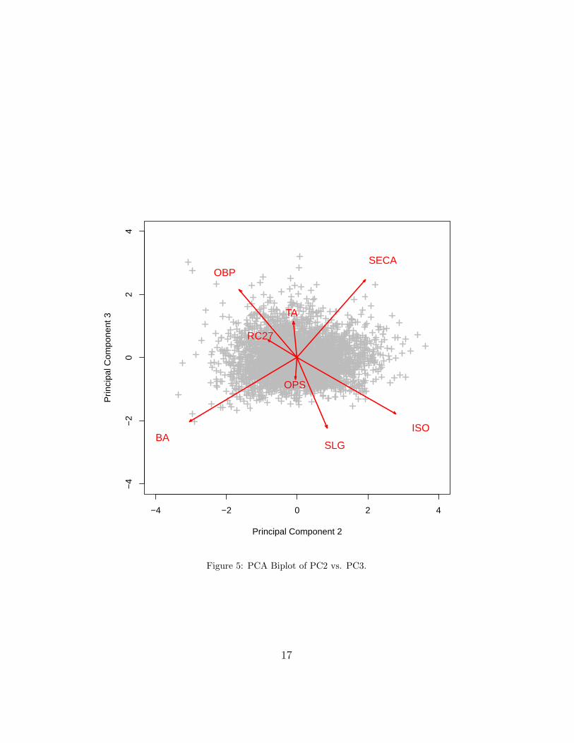
The factor loadings for the third principal component indicate that thethird principal component clearly separates OBP and SECA from BA, SLG,and ISO. The third component seems to separate those measures that dependon bases obtained via other sources (BB, HBP, and SB) from those measuresthat do not.

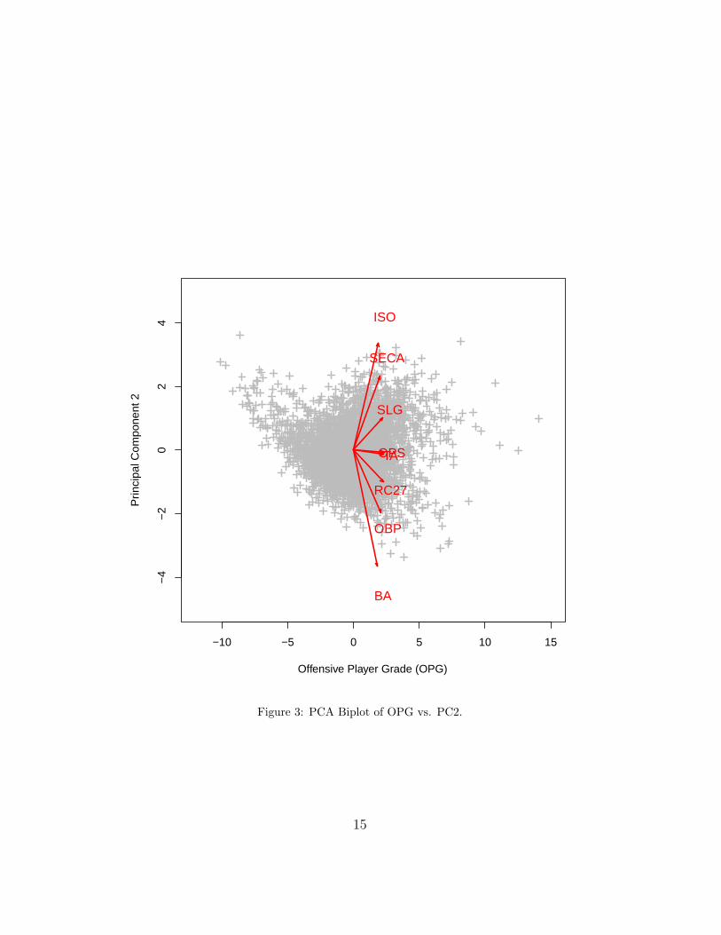
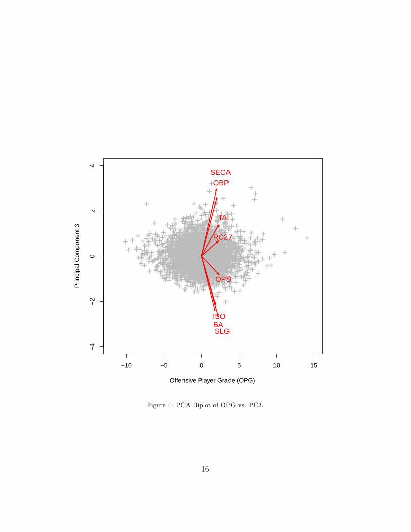
PCA is able to reduce the dimensionality of the data set from 3491 obser-vations on 8 variables to 3491 observations on 2 principal components whileretaining 93.72% of the sample variance, which is a very satisfactory result.Including the third principal component would retain 98.77% of the samplevariance. A PCA biplot gives us an accessible two-dimensional visualizationof the data. In Figures 3-5, PCA biplots display the 8-dimensional dataprojected down onto the lower-dimensional principal components.

The PCA projection of high-dimensional data onto a convenient lower-dimensional space also provides an opportunity for data segmentation. Seg-mentation will add detail and structure to the PCA biplots. In practice, it

14

−10 −5 0 5 10 15

−4

−2

02

4

Offensive Player Grade (OPG)

Prin

cipa

l Com

pone

nt 2

BA

OBP

SLG

OPSTA

ISO

SECA

RC27

Figure 3: PCA Biplot of OPG vs. PC2.

15

−10 −5 0 5 10 15

−4

−2

02

4

Offensive Player Grade (OPG)

Prin

cipa

l Com

pone

nt 3

BA

OBP

SLG

OPS

TA

ISO

SECA

RC27

Figure 4: PCA Biplot of OPG vs. PC3.

16

−4 −2 0 2 4

−4

−2

02

4

Principal Component 2

Prin

cipa

l Com

pone

nt 3

BA

OBP

SLG

OPS

TA

ISO

SECA

RC27

Figure 5: PCA Biplot of PC2 vs. PC3.

17

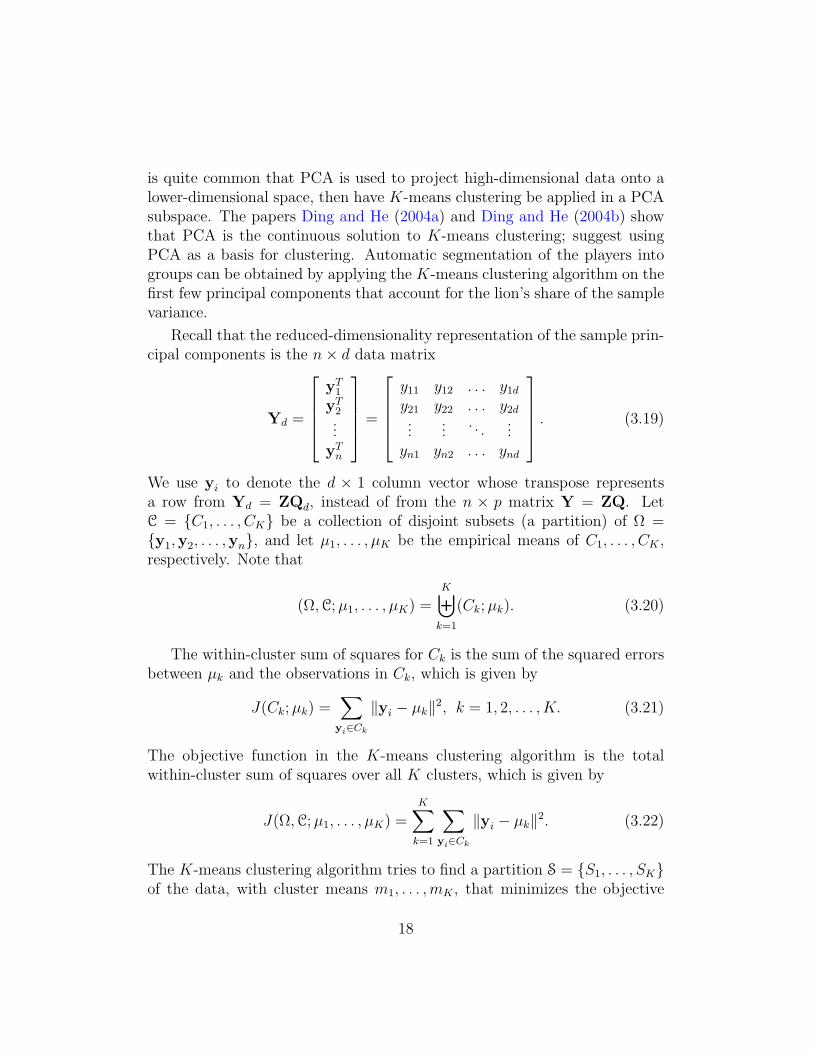
is quite common that PCA is used to project high-dimensional data onto alower-dimensional space, then have K-means clustering be applied in a PCAsubspace. The papers Ding and He (2004a) and Ding and He (2004b) showthat PCA is the continuous solution to K-means clustering; suggest usingPCA as a basis for clustering. Automatic segmentation of the players intogroups can be obtained by applying the K-means clustering algorithm on thefirst few principal components that account for the lion’s share of the samplevariance.

Recall that the reduced-dimensionality representation of the sample prin-cipal components is the n× d data matrix

Yd =

yT1

yT2...yTn

=

y11 y12 . . . y1dy21 y22 . . . y2d...

.... . .

...yn1 yn2 . . . ynd

. (3.19)

We use yi to denote the d × 1 column vector whose transpose representsa row from Yd = ZQd, instead of from the n × p matrix Y = ZQ. LetC = C1, . . . , CK be a collection of disjoint subsets (a partition) of Ω =y1,y2, . . . ,yn, and let µ1, . . . , µK be the empirical means of C1, . . . , CK ,respectively. Note that

(Ω,C;µ1, . . . , µK) =K⊎k=1

(Ck;µk). (3.20)

The within-cluster sum of squares for Ck is the sum of the squared errorsbetween µk and the observations in Ck, which is given by

J(Ck;µk) =∑yi∈Ck

∥yi − µk∥2, k = 1, 2, . . . , K. (3.21)

The objective function in the K-means clustering algorithm is the totalwithin-cluster sum of squares over all K clusters, which is given by

J(Ω,C;µ1, . . . , µK) =K∑k=1

∑yi∈Ck

∥yi − µk∥2. (3.22)

The K-means clustering algorithm tries to find a partition S = S1, . . . , SKof the data, with cluster means m1, . . . ,mK , that minimizes the objective

18

function, i.e.

J(Ω, S;m1, . . . ,mK) = minK

minµ1,...,µK

K∑k=1

∑yi∈Ck

∥yi − µk∥2. (3.23)

A cluster becomes more homogeneous as its within-cluster sum of squares de-creases; clustering of the sample observations gets better as the total within-cluster sum of squares decreases.

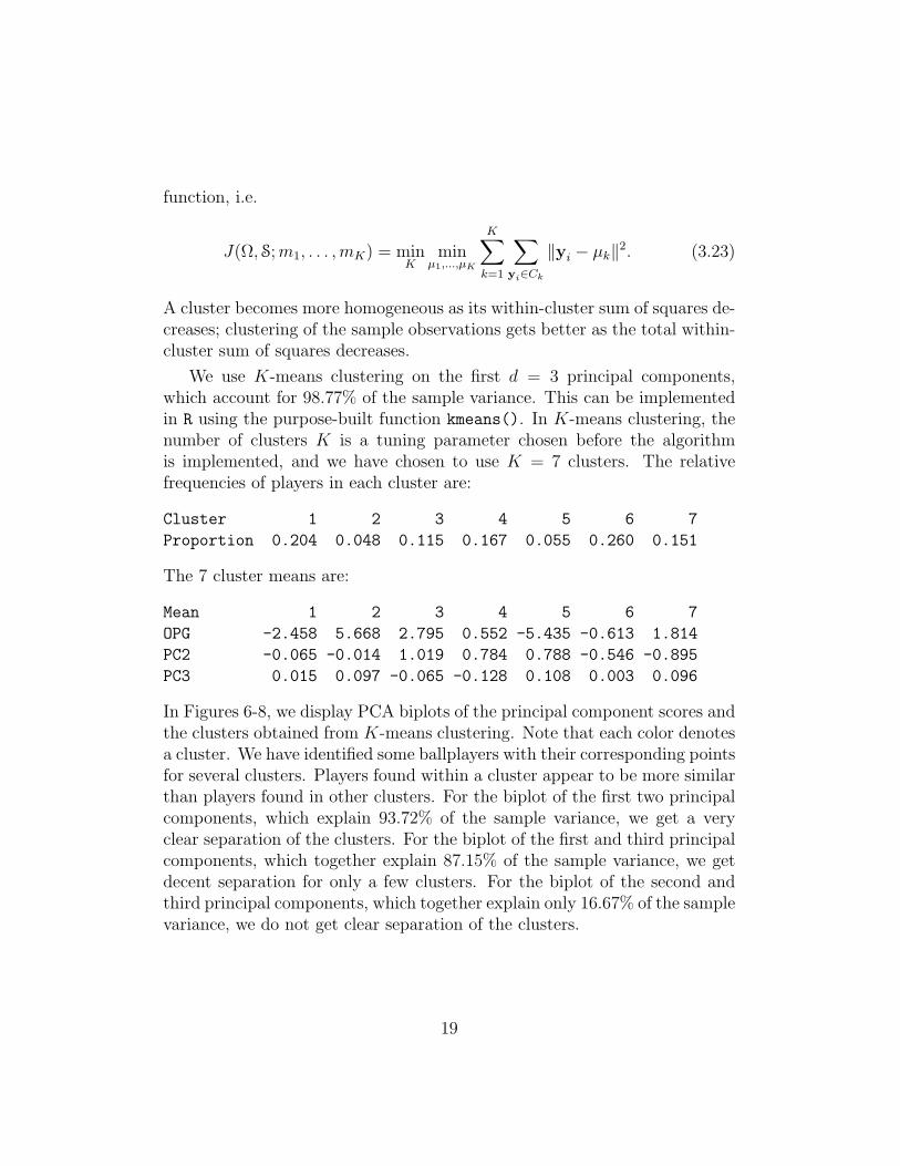
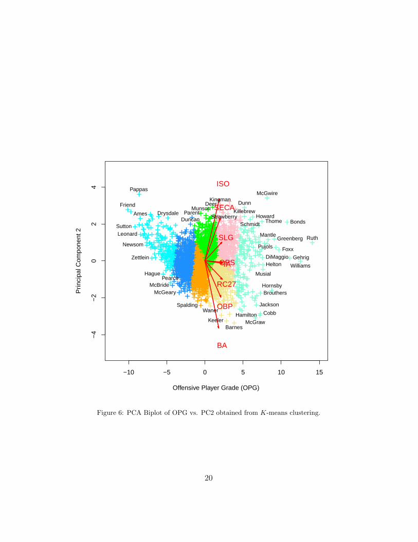
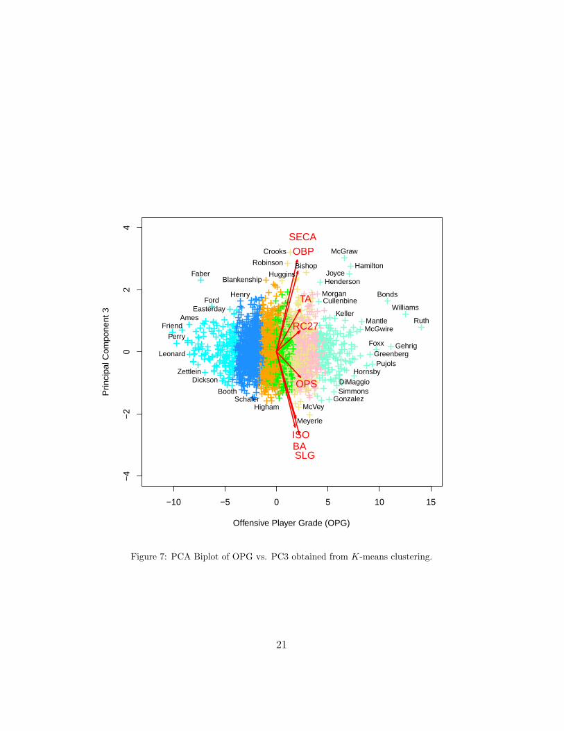
We use K-means clustering on the first d = 3 principal components,which account for 98.77% of the sample variance. This can be implementedin R using the purpose-built function kmeans(). In K-means clustering, thenumber of clusters K is a tuning parameter chosen before the algorithmis implemented, and we have chosen to use K = 7 clusters. The relativefrequencies of players in each cluster are:

Cluster 1 2 3 4 5 6 7

Proportion 0.204 0.048 0.115 0.167 0.055 0.260 0.151

The 7 cluster means are:

Mean 1 2 3 4 5 6 7

OPG -2.458 5.668 2.795 0.552 -5.435 -0.613 1.814

PC2 -0.065 -0.014 1.019 0.784 0.788 -0.546 -0.895

PC3 0.015 0.097 -0.065 -0.128 0.108 0.003 0.096

In Figures 6-8, we display PCA biplots of the principal component scores andthe clusters obtained from K-means clustering. Note that each color denotesa cluster. We have identified some ballplayers with their corresponding pointsfor several clusters. Players found within a cluster appear to be more similarthan players found in other clusters. For the biplot of the first two principalcomponents, which explain 93.72% of the sample variance, we get a veryclear separation of the clusters. For the biplot of the first and third principalcomponents, which together explain 87.15% of the sample variance, we getdecent separation for only a few clusters. For the biplot of the second andthird principal components, which together explain only 16.67% of the samplevariance, we do not get clear separation of the clusters.

19

−10 −5 0 5 10 15

−4

−2

02

4

Offensive Player Grade (OPG)

Prin

cipa

l Com

pone

nt 2

BA

OBP

SLG

OPSTA

ISO

SECA

RC27

Ames

Barnes

Bonds

Brouthers

Cobb

Deer

DiMaggio

DrysdaleDuncan

Dunn

Foxx

Friend

Gehrig

Greenberg

Hague

Hamilton

Helton

Hornsby

Howard

Jackson

Keeler

Killebrew

Kingman

Leonard Mantle

McBrideMcGeary

McGraw

McGwire

Munson

Musial

Newsom

Pappas

Parent

Pearce

Pujols

Ruth

Schmidt

Spalding

Strawberry

SuttonThome

Waner

Williams

Zettlein

Figure 6: PCA Biplot of OPG vs. PC2 obtained from K-means clustering.

20

−10 −5 0 5 10 15

−4

−2

02

4

Offensive Player Grade (OPG)

Prin

cipa

l Com

pone

nt 3

BA

OBP

SLG

OPS

TA

ISO

SECA

RC27Ames

Bishop

Blankenship

Bonds

Booth

Crooks

Cullenbine

Dickson DiMaggio

Easterday

Faber

Ford

Foxx

Friend

Gehrig

Gonzalez

Greenberg

Hamilton

Henderson

Henry

Higham

Hornsby

Huggins Joyce

Keller

Leonard

Mantle

McGraw

McGwire

McVey

Meyerle

Morgan

Perry

Pujols

Robinson

Ruth

SchaferSimmons

Williams

Zettlein

Figure 7: PCA Biplot of OPG vs. PC3 obtained from K-means clustering.

21

−4 −2 0 2 4

−4

−2

02

4

Principal Component 2

Prin

cipa

l Com

pone

nt 3

BA

OBP

SLG

OPS

TA

ISO

SECA

RC27

Andrews

Armas

Ashburn

Balboni

Barnes

Bassler

BishopBlankenship

BranyanBurkett

Childs

Cobb

Collins

Crooks

Cust

Dunn

Faber

GonzalezHall

HamiltonHuggins

Joyce

Keeler

Kingman

Lake

McGraw

McGwire

McVey

Meyerle

Nordhagen

Pappas

Phelps

PikeQuinn

Robinson

Spalding

Taylor

Tenace

Thames

Thomas

Waner

Westrum

Figure 8: PCA Biplot of PC2 vs. PC3 obtained from K-means clustering.

22

4. Offensive Player Grade (OPG)

This section is devoted to the PCA derived measure Offensive PlayerGrade. Recall that the formula for OPG is given by

OPG = 0.30

(BA− 0.263

0.027

)+ 0.35

(OBP− 0.326

0.036

)+ 0.37

(SLG− 0.380

0.064

)+ 0.39

(OPS− 0.706

0.094

)+ 0.38

(TA− 0.651

0.129

)+ 0.32

(ISO− 0.118

0.049

)+ 0.34

(SECA− 0.222

0.072

)+ 0.38

(RC27− 4.569

1.322

). (4.1)

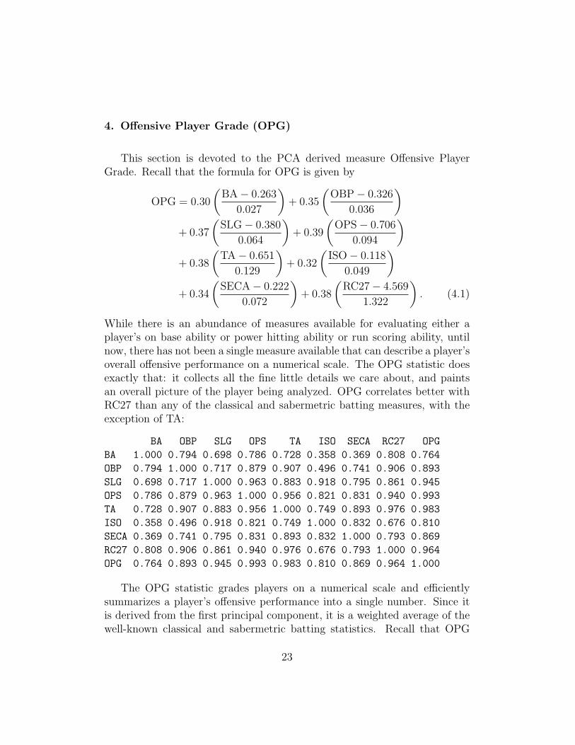
While there is an abundance of measures available for evaluating either aplayer’s on base ability or power hitting ability or run scoring ability, untilnow, there has not been a single measure available that can describe a player’soverall offensive performance on a numerical scale. The OPG statistic doesexactly that: it collects all the fine little details we care about, and paintsan overall picture of the player being analyzed. OPG correlates better withRC27 than any of the classical and sabermetric batting measures, with theexception of TA:

BA OBP SLG OPS TA ISO SECA RC27 OPG

BA 1.000 0.794 0.698 0.786 0.728 0.358 0.369 0.808 0.764

OBP 0.794 1.000 0.717 0.879 0.907 0.496 0.741 0.906 0.893

SLG 0.698 0.717 1.000 0.963 0.883 0.918 0.795 0.861 0.945

OPS 0.786 0.879 0.963 1.000 0.956 0.821 0.831 0.940 0.993

TA 0.728 0.907 0.883 0.956 1.000 0.749 0.893 0.976 0.983

ISO 0.358 0.496 0.918 0.821 0.749 1.000 0.832 0.676 0.810

SECA 0.369 0.741 0.795 0.831 0.893 0.832 1.000 0.793 0.869

RC27 0.808 0.906 0.861 0.940 0.976 0.676 0.793 1.000 0.964

OPG 0.764 0.893 0.945 0.993 0.983 0.810 0.869 0.964 1.000

The OPG statistic grades players on a numerical scale and efficientlysummarizes a player’s offensive performance into a single number. Since itis derived from the first principal component, it is a weighted average of thewell-known classical and sabermetric batting statistics. Recall that OPG

23

= −PC1, so larger positive OPG scores indicate better offensive players;larger negative OPG scores indicate poorer offensive players; OPG scores ina neighborhood of zero indicate an average offensive player. Within reason,one can compare the offensive performances between two comparable playerson the basis of OPG.

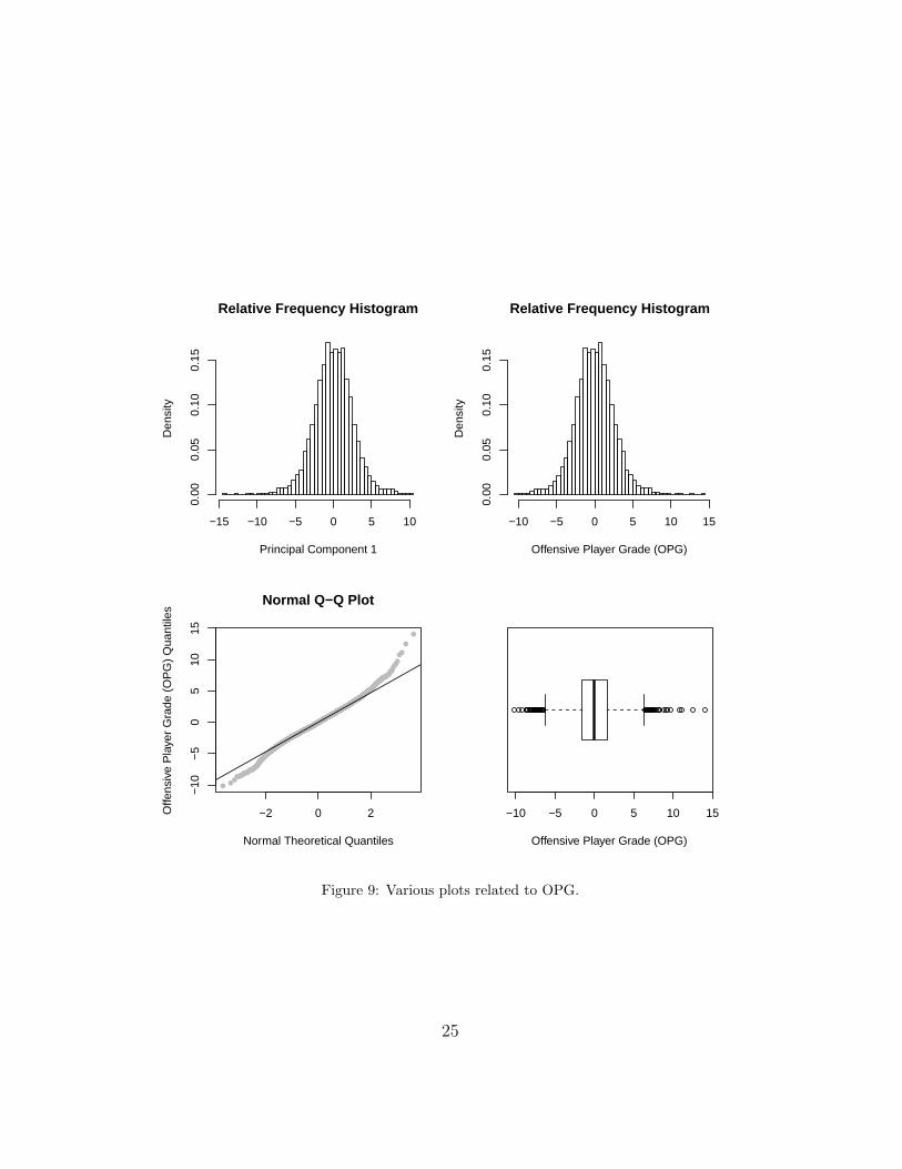
To get the most out of the OPG statistic, a partition of the range of valuesfor OPG should be established in a meaningful way. One might think aboutusing the Empirical Rule of the Normal distribution (the so-called “Three-Sigma Rule”) to establish a meaningful partition. The relative frequencyhistogram of the OPG scores appears to show an approximate Normal dis-tribution, but this may be misleading. In fact, the non-linearity in the Q-Qplot indicates an obvious departure from Normality. Moreover, the Shapiro-Wilk test concludes that the OPG scores are not distributed according tothe Normal distribution (the p-value is smaller than 0.01).

Since the Empirical Rule may not be reliable, a sensible and robust so-lution is to partition the range of values for OPG according to the samplequantiles. For example, we can compute the sample deciles of the OPGscores:

0% 10% 20% 30% 40% 50% 60% 70% 80% 90% 100%

-10.1 -3.0 -2.0 -1.3 -0.7 0.0 0.6 1.2 2.0 3.1 14.1

Then a possible partition of the range for OPG might go like this:

A = [3, Infinity),

B = [2, 3),

C = (-2, 2),

D = (-3, -2],

Fail = (-Infinity, -3].

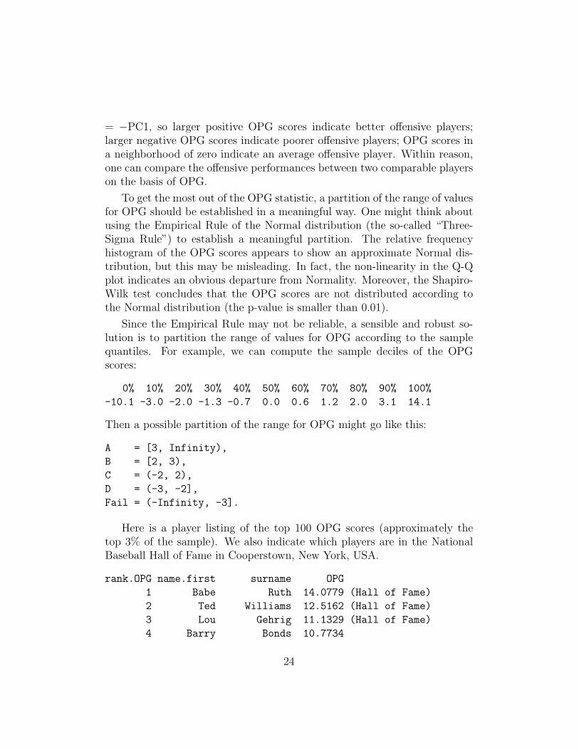
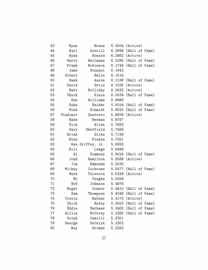
Here is a player listing of the top 100 OPG scores (approximately thetop 3% of the sample). We also indicate which players are in the NationalBaseball Hall of Fame in Cooperstown, New York, USA.

rank.OPG name.first surname OPG

1 Babe Ruth 14.0779 (Hall of Fame)

2 Ted Williams 12.5162 (Hall of Fame)

3 Lou Gehrig 11.1329 (Hall of Fame)

4 Barry Bonds 10.7734

24

Relative Frequency Histogram

Principal Component 1

Den

sity

−15 −10 −5 0 5 10

0.00

0.05

0.10

0.15

Relative Frequency Histogram

Offensive Player Grade (OPG)

Den

sity

−10 −5 0 5 10 15

0.00

0.05

0.10

0.15

−2 0 2

−10

−5

05

1015

Normal Q−Q Plot

Normal Theoretical Quantiles

Offe

nsiv

e P

laye

r G

rade

(O

PG

) Q

uant

iles

−10 −5 0 5 10 15

Offensive Player Grade (OPG)

Figure 9: Various plots related to OPG.

25

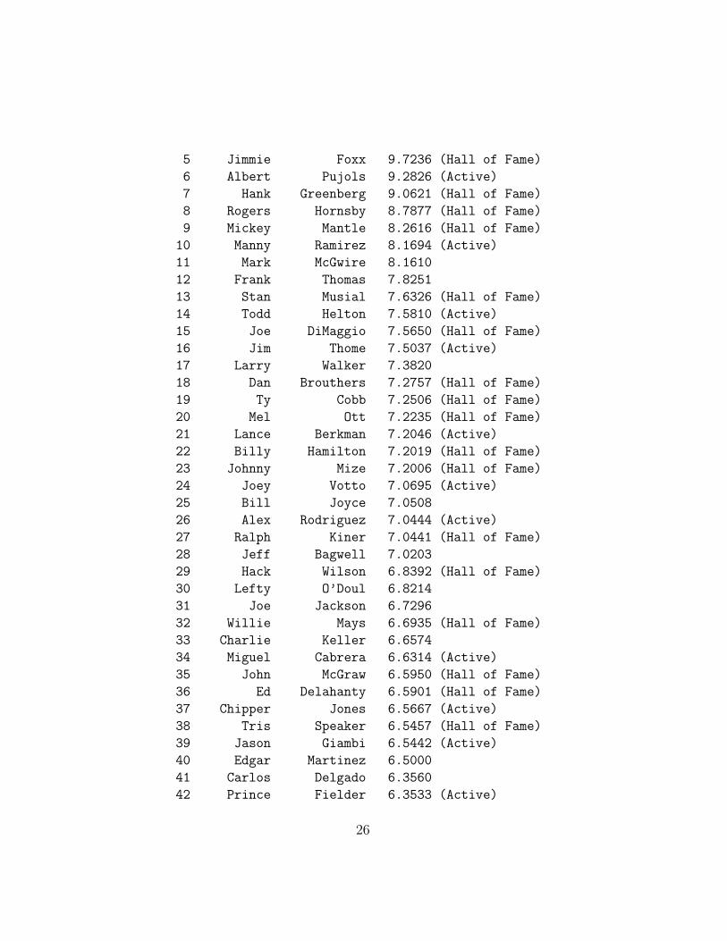
5 Jimmie Foxx 9.7236 (Hall of Fame)

6 Albert Pujols 9.2826 (Active)

7 Hank Greenberg 9.0621 (Hall of Fame)

8 Rogers Hornsby 8.7877 (Hall of Fame)

9 Mickey Mantle 8.2616 (Hall of Fame)

10 Manny Ramirez 8.1694 (Active)

11 Mark McGwire 8.1610

12 Frank Thomas 7.8251

13 Stan Musial 7.6326 (Hall of Fame)

14 Todd Helton 7.5810 (Active)

15 Joe DiMaggio 7.5650 (Hall of Fame)

16 Jim Thome 7.5037 (Active)

17 Larry Walker 7.3820

18 Dan Brouthers 7.2757 (Hall of Fame)

19 Ty Cobb 7.2506 (Hall of Fame)

20 Mel Ott 7.2235 (Hall of Fame)

21 Lance Berkman 7.2046 (Active)

22 Billy Hamilton 7.2019 (Hall of Fame)

23 Johnny Mize 7.2006 (Hall of Fame)

24 Joey Votto 7.0695 (Active)

25 Bill Joyce 7.0508

26 Alex Rodriguez 7.0444 (Active)

27 Ralph Kiner 7.0441 (Hall of Fame)

28 Jeff Bagwell 7.0203

29 Hack Wilson 6.8392 (Hall of Fame)

30 Lefty O’Doul 6.8214

31 Joe Jackson 6.7296

32 Willie Mays 6.6935 (Hall of Fame)

33 Charlie Keller 6.6574

34 Miguel Cabrera 6.6314 (Active)

35 John McGraw 6.5950 (Hall of Fame)

36 Ed Delahanty 6.5901 (Hall of Fame)

37 Chipper Jones 6.5667 (Active)

38 Tris Speaker 6.5457 (Hall of Fame)

39 Jason Giambi 6.5442 (Active)

40 Edgar Martinez 6.5000

41 Carlos Delgado 6.3560

42 Prince Fielder 6.3533 (Active)

26

43 Ryan Braun 6.3004 (Active)

44 Earl Averill 6.2896 (Hall of Fame)

45 Ryan Howard 6.2862 (Active)

46 Harry Heilmann 6.2295 (Hall of Fame)

47 Frank Robinson 6.1748 (Hall of Fame)

48 Jake Stenzel 6.1642

49 Albert Belle 6.1516

50 Hank Aaron 6.1138 (Hall of Fame)

51 David Ortiz 6.1035 (Active)

52 Matt Holliday 6.0632 (Active)

53 Chuck Klein 6.0539 (Hall of Fame)

54 Ken Williams 5.9986

55 Duke Snider 5.9154 (Hall of Fame)

56 Mike Schmidt 5.9030 (Hall of Fame)

57 Vladimir Guerrero 5.8839 (Active)

58 Babe Herman 5.8767

59 Dick Allen 5.7682

60 Gary Sheffield 5.7568

61 Brian Giles 5.7136

62 Mike Piazza 5.7051

63 Ken Griffey, Jr. 5.6926

64 Bill Lange 5.6499

65 Al Simmons 5.6024 (Hall of Fame)

66 Josh Hamilton 5.5588 (Active)

67 Jim Edmonds 5.5535

68 Mickey Cochrane 5.5477 (Hall of Fame)

69 Mark Teixeira 5.5338 (Active)

70 Mo Vaughn 5.5059

71 Bob Johnson 5.4876

72 Roger Connor 5.4410 (Hall of Fame)

73 Sam Thompson 5.4048 (Hall of Fame)

74 Travis Hafner 5.3173 (Active)

75 Chick Hafey 5.3053 (Hall of Fame)

76 Eddie Mathews 5.2405 (Hall of Fame)

77 Willie McCovey 5.2385 (Hall of Fame)

78 Dolph Camilli 5.2351

79 George Selkirk 5.2302

80 Ray Grimes 5.2292

27

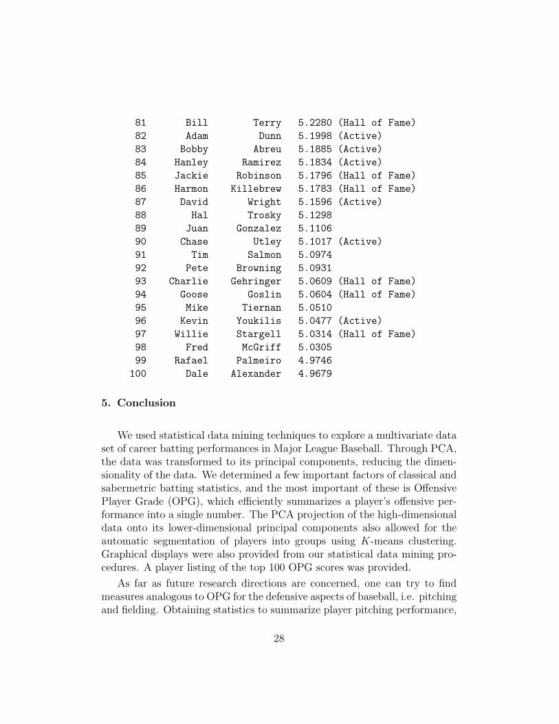
81 Bill Terry 5.2280 (Hall of Fame)

82 Adam Dunn 5.1998 (Active)

83 Bobby Abreu 5.1885 (Active)

84 Hanley Ramirez 5.1834 (Active)

85 Jackie Robinson 5.1796 (Hall of Fame)

86 Harmon Killebrew 5.1783 (Hall of Fame)

87 David Wright 5.1596 (Active)

88 Hal Trosky 5.1298

89 Juan Gonzalez 5.1106

90 Chase Utley 5.1017 (Active)

91 Tim Salmon 5.0974

92 Pete Browning 5.0931

93 Charlie Gehringer 5.0609 (Hall of Fame)

94 Goose Goslin 5.0604 (Hall of Fame)

95 Mike Tiernan 5.0510

96 Kevin Youkilis 5.0477 (Active)

97 Willie Stargell 5.0314 (Hall of Fame)

98 Fred McGriff 5.0305

99 Rafael Palmeiro 4.9746

100 Dale Alexander 4.9679

5. Conclusion

We used statistical data mining techniques to explore a multivariate dataset of career batting performances in Major League Baseball. Through PCA,the data was transformed to its principal components, reducing the dimen-sionality of the data. We determined a few important factors of classical andsabermetric batting statistics, and the most important of these is OffensivePlayer Grade (OPG), which efficiently summarizes a player’s offensive per-formance into a single number. The PCA projection of the high-dimensionaldata onto its lower-dimensional principal components also allowed for theautomatic segmentation of players into groups using K-means clustering.Graphical displays were also provided from our statistical data mining pro-cedures. A player listing of the top 100 OPG scores was provided.

As far as future research directions are concerned, one can try to findmeasures analogous to OPG for the defensive aspects of baseball, i.e. pitchingand fielding. Obtaining statistics to summarize player pitching performance,

28

and player fielding performance are of great interest. These might be calledPlayer Pitching Grade (PPG) and Player Fielding Grade (PFG), respectively.The methods employed here can be applied to other sports, e.g. basketball,football, ice hockey, etc. Statistical data mining alternatives to PCA includeIndependent Components Analysis (ICA) and Projection Pursuit (PP), cf.Hastie et al. (2009).

Albert, J., Bennett, J., 2001. Curve Ball: Baseball, Statistics, and the Roleof Chance in the Game. Copernicus Books.

Biau, G., Devroye, L., Lugosi, G., 2008. On the performance of clusteringin Hilbert spaces. IEEE Transactions on Information Theory 54, No. 2,781–790.

Bock, H., 2008. Origins and extensions of the k-means algorithm in clusteranalysis. Electronic Journal for History of Probability and Statistics 4, No.2.

Ding, C., He, X., 2004a. K-means clustering via principal component analy-sis. In: Proceedings of the 21st International Conference on Machine Learn-ing. Vol. 69. ACM Press, pp. 225232.

Ding, C., He, X., 2004b. Principal component analysis and effective K-meansclustering. In: Proceedings of the 2004 SIAM International Conference onData Mining. Vol. 2, No. 2. Society for Industrial and Applied Mathemat-ics, pp. 497–501.

Hastie, T., Tibshirani, R., Friedman, J., 2009. The Elements of StatisticalLearning: Data Mining, Inference, and Prediction, 2nd Edition. Springer.

Izenman, A. J., 2008. Modern Multivariate Statistical Techniques: Regres-sion, Classification, and Manifold Learning. Springer.

Jain, A., 2010. Data clustering: 50 years beyond K-means. Pattern Recogni-tion Letters 31, 651–666.

Johnson, R. A., Wichern, D. W., 2007. Applied Multivariate Statistical Anal-ysis, Sixth Edition. Prentice Hall.

Keri, J., 2007. Baseball Between the Numbers: Why Everything You Knowabout the Game Is Wrong. Perseus Publishing.

29

Melnykov, V., Maitra, R., 2010. Finite mixture models and model-basedclustering. Statistics Surveys 4, 80–116.

R Development Core Team, 2011. R: A Language and Environment for Sta-tistical Computing. R Foundation for Statistical Computing, Vienna, Aus-tria, ISBN 3-900051-07-0.URL http://www.R-project.org/

Tuffery, S., 2011. Data Mining and Statistics for Decision Making. Wiley.

Wu, X., Kumar, V., Quinlan, J. R., Ghosh, J., Yang, Q., Motoda, H.,McLachlan, G. J., Ng, A., Liu, B., Yu, P. S., Zhou, Z., Steinbach, M., Hand,D. J., Steinberg, D., 2008. Top 10 algorithms in data mining. Knowledgeand Information Systems 14, 1–37.

30