Embed Size (px)
Citation preview

Data Mining 2017Text Classification
Naive Bayes
Ad Feelders
Universiteit Utrecht
October 18, 2017
Ad Feelders ( Universiteit Utrecht ) Data Mining October 18, 2017 1 / 44
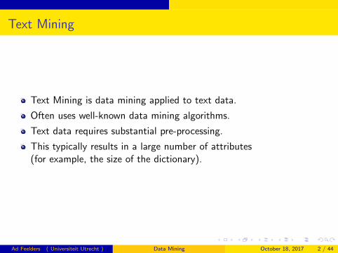
Text Mining
Text Mining is data mining applied to text data.
Often uses well-known data mining algorithms.
Text data requires substantial pre-processing.
This typically results in a large number of attributes(for example, the size of the dictionary).
Ad Feelders ( Universiteit Utrecht ) Data Mining October 18, 2017 2 / 44

Text Classification
Predict the class(es) of text documents.
Can be single-label or multi-label.
Multi-label classification is often performed by building multiplebinary classifiers (one for each possible class).
Examples of text classification:
topics of news articles,spam/no spam for e-mail messages,sentiment analysis (e.g. positive/negative review),opinion spam (e.g. fake reviews),music genre from song lyrics
Ad Feelders ( Universiteit Utrecht ) Data Mining October 18, 2017 3 / 44
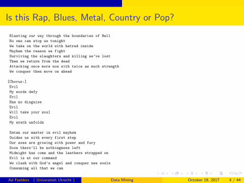
Is this Rap, Blues, Metal, Country or Pop?
Blasting our way through the boundaries of Hell
No one can stop us tonight
We take on the world with hatred inside
Mayhem the reason we fight
Surviving the slaughters and killing we’ve lost
Then we return from the dead
Attacking once more now with twice as much strength
We conquer then move on ahead
[Chorus:]
Evil
My words defy
Evil
Has no disguise
Evil
Will take your soul
Evil
My wrath unfolds
Satan our master in evil mayhem
Guides us with every first step
Our axes are growing with power and fury
Soon there’ll be nothingness left
Midnight has come and the leathers strapped on
Evil is at our command
We clash with God’s angel and conquer new souls
Consuming all that we can
Ad Feelders ( Universiteit Utrecht ) Data Mining October 18, 2017 4 / 44
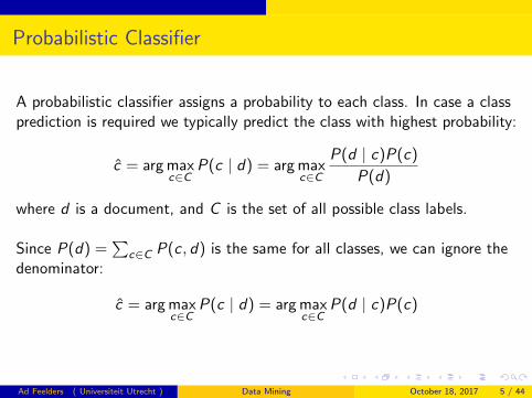
Probabilistic Classifier
A probabilistic classifier assigns a probability to each class. In case a classprediction is required we typically predict the class with highest probability:
c = arg maxc∈C
P(c | d) = arg maxc∈C
P(d | c)P(c)
P(d)
where d is a document, and C is the set of all possible class labels.
Since P(d) =∑
c∈C P(c , d) is the same for all classes, we can ignore thedenominator:
c = arg maxc∈C
P(c | d) = arg maxc∈C
P(d | c)P(c)
Ad Feelders ( Universiteit Utrecht ) Data Mining October 18, 2017 5 / 44
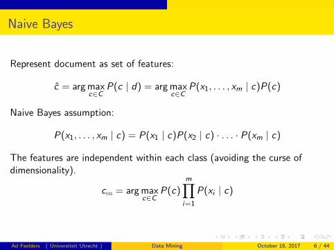
Naive Bayes
Represent document as set of features:
c = arg maxc∈C
P(c | d) = arg maxc∈C
P(x1, . . . , xm | c)P(c)
Naive Bayes assumption:
P(x1, . . . , xm | c) = P(x1 | c)P(x2 | c) · . . . · P(xm | c)
The features are independent within each class (avoiding the curse ofdimensionality).
cnb = arg maxc∈C
P(c)m∏
i=1
P(xi | c)
Ad Feelders ( Universiteit Utrecht ) Data Mining October 18, 2017 6 / 44
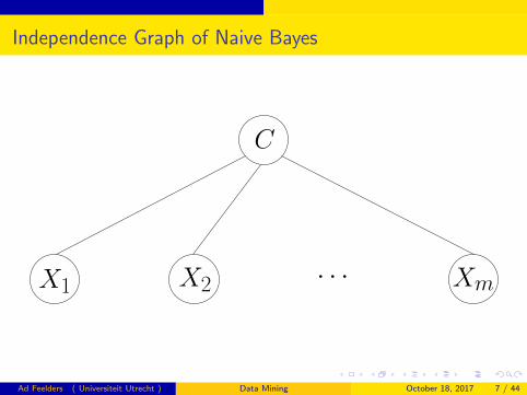
Independence Graph of Naive Bayes
C
X1 X2 Xm· · ·
Ad Feelders ( Universiteit Utrecht ) Data Mining October 18, 2017 7 / 44
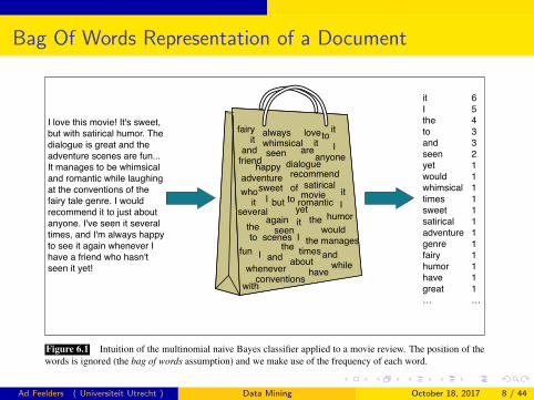
Bag Of Words Representation of a Document
6.1 • NAIVE BAYES CLASSIFIERS 3
6.1 Naive Bayes Classifiers
In this section we introduce the multinomial naive Bayes classifier, so called be-naive Bayesclassifier
cause it is a Bayesian classifier that makes a simplifying (naive) assumption abouthow the features interact.
The intuition of the classifier is shown in Fig. 6.1. We represent a text documentas if it were a bag-of-words, that is, an unordered set of words with their positionbag-of-words
ignored, keeping only their frequency in the document. In the example in the figure,instead of representing the word order in all the phrases like “I love this movie” and“I would recommend it”, we simply note that the word I occurred 5 times in theentire excerpt, the word it 6 times, the words love, recommend, and movie once, andso on.
it
it
itit
it
it
I
I
I
I
I
love
recommend
movie
thethe
the
the
to
to
to
and
andand
seen
seen
yet
would
with
who
whimsical
whilewhenever
times
sweet
several
scenes
satirical
romanticof
manages
humor
have
happy
fun
friend
fairy
dialogue
but
conventions
areanyone
adventure
always
again
about
I love this movie! It's sweet, but with satirical humor. The dialogue is great and the adventure scenes are fun... It manages to be whimsical and romantic while laughing at the conventions of the fairy tale genre. I would recommend it to just about anyone. I've seen it several times, and I'm always happy to see it again whenever I have a friend who hasn't seen it yet!
it Ithetoandseenyetwouldwhimsicaltimessweetsatiricaladventuregenrefairyhumorhavegreat…
6 54332111111111111…
Figure 6.1 Intuition of the multinomial naive Bayes classifier applied to a movie review. The position of thewords is ignored (the bag of words assumption) and we make use of the frequency of each word.
Naive Bayes is a probabilistic classifier, meaning that for a document d, out ofall classes c ∈C the classifier returns the class c which has the maximum posteriorprobability given the document. In Eq. 6.1 we use the hat notation ˆ to mean “ourˆ
estimate of the correct class”.
c = argmaxc∈C
P(c|d) (6.1)
This idea of Bayesian inference has been known since the work of Bayes (1763),Bayesianinference
and was first applied to text classification by Mosteller and Wallace (1964). The in-tuition of Bayesian classification is to use Bayes’ rule to transform Eq. 6.1 into otherprobabilities that have some useful properties. Bayes’ rule is presented in Eq. 6.2;it gives us a way to break down any conditional probability P(x|y) into three other
Ad Feelders ( Universiteit Utrecht ) Data Mining October 18, 2017 8 / 44
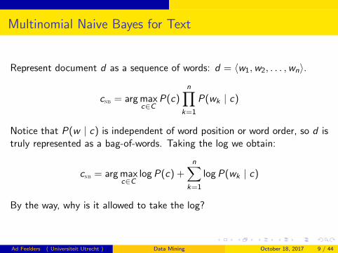
Multinomial Naive Bayes for Text
Represent document d as a sequence of words: d = 〈w1,w2, . . . ,wn〉.
cnb = arg maxc∈C
P(c)n∏
k=1
P(wk | c)
Notice that P(w | c) is independent of word position or word order, so d istruly represented as a bag-of-words. Taking the log we obtain:
cnb = arg maxc∈C
logP(c) +n∑
k=1
logP(wk | c)
By the way, why is it allowed to take the log?
Ad Feelders ( Universiteit Utrecht ) Data Mining October 18, 2017 9 / 44
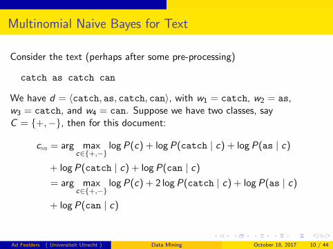
Multinomial Naive Bayes for Text
Consider the text (perhaps after some pre-processing)
catch as catch can
We have d = 〈catch, as, catch, can〉, with w1 = catch, w2 = as,w3 = catch, and w4 = can. Suppose we have two classes, sayC = {+,−}, then for this document:
cnb = arg maxc∈{+,−}
logP(c) + logP(catch | c) + logP(as | c)
+ logP(catch | c) + logP(can | c)
= arg maxc∈{+,−}
logP(c) + 2 logP(catch | c) + logP(as | c)
+ logP(can | c)
Ad Feelders ( Universiteit Utrecht ) Data Mining October 18, 2017 10 / 44
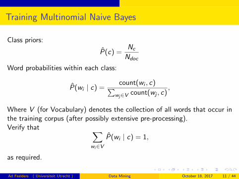
Training Multinomial Naive Bayes
Class priors:
P(c) =Nc
Ndoc
Word probabilities within each class:
P(wi | c) =count(wi , c)∑
wj∈V count(wj , c),
Where V (for Vocabulary) denotes the collection of all words that occur inthe training corpus (after possibly extensive pre-processing).Verify that ∑
wi∈VP(wi | c) = 1,
as required.
Ad Feelders ( Universiteit Utrecht ) Data Mining October 18, 2017 11 / 44
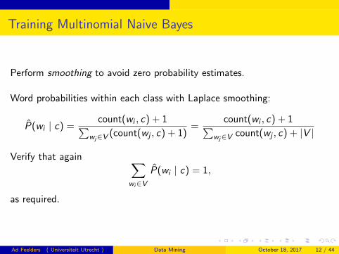
Training Multinomial Naive Bayes
Perform smoothing to avoid zero probability estimates.
Word probabilities within each class with Laplace smoothing:
P(wi | c) =count(wi , c) + 1∑
wj∈V (count(wj , c) + 1)=
count(wi , c) + 1∑wj∈V count(wj , c) + |V |
Verify that again ∑
wi∈VP(wi | c) = 1,
as required.
Ad Feelders ( Universiteit Utrecht ) Data Mining October 18, 2017 12 / 44
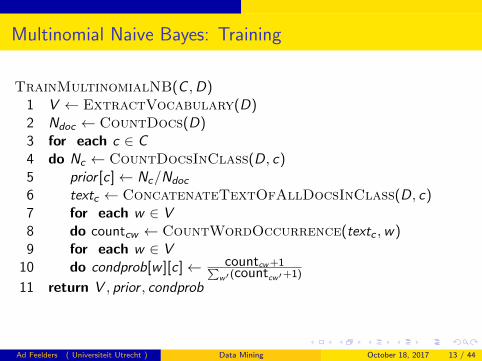
Multinomial Naive Bayes: Training
TrainMultinomialNB(C ,D)1 V ← ExtractVocabulary(D)2 Ndoc ← CountDocs(D)3 for each c ∈ C4 do Nc ← CountDocsInClass(D, c)5 prior [c]← Nc/Ndoc
6 textc ← ConcatenateTextOfAllDocsInClass(D, c)7 for each w ∈ V8 do countcw ← CountWordOccurrence(textc ,w)9 for each w ∈ V
10 do condprob[w ][c]← countcw+1∑w′ (countcw′+1)
11 return V , prior , condprob
Ad Feelders ( Universiteit Utrecht ) Data Mining October 18, 2017 13 / 44

Multinomial Naive Bayes: Prediction
Predict the class of a document d .
ApplyMultinomialNB(C ,V , prior , condprob, d)1 W ← ExtractWordOccurrencesFromDoc(V , d)2 for each c ∈ C3 do score[c]← log prior [c]4 for each w ∈W5 do score[c]+ = log condprob[w ][c]6 return arg maxc∈C score[c]
Ad Feelders ( Universiteit Utrecht ) Data Mining October 18, 2017 14 / 44
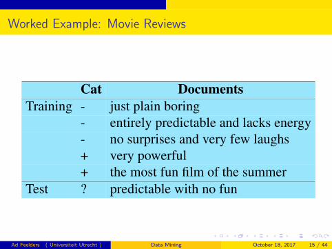
Worked Example: Movie Reviews
6 CHAPTER 6 • NAIVE BAYES AND SENTIMENT CLASSIFICATION
P(“fantastic”|positive) =count(“fantastic”,positive)∑
w∈V count(w,positive)= 0 (6.13)
But since naive Bayes naively multiplies all the feature likelihoods together, zeroprobabilities in the likelihood term for any class will cause the probability of theclass to be zero, no matter the other evidence!
The simplest solution is the add-one (Laplace) smoothing introduced in Chap-ter 4. While Laplace smoothing is usually replaced by more sophisticated smoothingalgorithms in language modeling, it is commonly used in naive Bayes text catego-rization:
P(wi|c) =count(wi,c)+1∑
w∈V (count(w,c)+1)=
count(wi,c)+1(∑w∈V count(w,c)
)+ |V | (6.14)
Note once again that it is a crucial that the vocabulary V consists of the unionof all the word types in all classes, not just the words in one class c (try to convinceyourself why this must be true; see the exercise at the end of the chapter).
What do we do about words that occur in our test data but are not in our vocab-ulary at all because they did not occur in any training document in any class? Thestandard solution for such unknown words is to ignore such words—remove themfrom the test document and not include any probability for them at all.
Finally, some systems choose to completely ignore another class of words: stopwords, very frequent words like the and a. This can be done by sorting the vocabu-stop words
lary by frequency in the training set, and defining the top 10–100 vocabulary entriesas stop words, or alternatively by using one of the many pre-defined stop word listavailable online. Then every instance of these stop words are simply removed fromboth training and test documents as if they had never occurred. In most text classi-fication applications, however, using a stop word list doesn’t improve performance,and so it is more common to make use of the entire vocabulary and not use a stopword list.
Fig. 6.2 shows the final algorithm.
6.3 Worked example
Let’s walk through an example of training and testing naive Bayes with add-onesmoothing. We’ll use a sentiment analysis domain with the two classes positive(+) and negative (-), and take the following miniature training and test documentssimplified from actual movie reviews.
Cat DocumentsTraining - just plain boring
- entirely predictable and lacks energy- no surprises and very few laughs+ very powerful+ the most fun film of the summer
Test ? predictable with no fun
The prior P(c) for the two classes is computed via Eq. 6.11 as NcNdoc
:
Ad Feelders ( Universiteit Utrecht ) Data Mining October 18, 2017 15 / 44
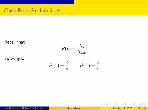
Class Prior Probabilities
Recall that:
P(c) =Nc
Ndoc
So we get:
P(+) =2
5P(−) =
3
5
Ad Feelders ( Universiteit Utrecht ) Data Mining October 18, 2017 16 / 44
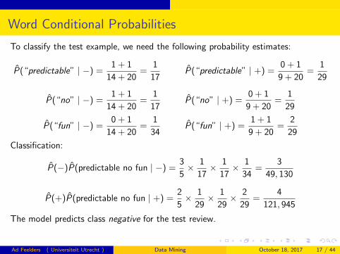
Word Conditional Probabilities
To classify the test example, we need the following probability estimates:
P(“predictable” | −) =1 + 1
14 + 20=
1
17P(“predictable” | +) =
0 + 1
9 + 20=
1
29
P(“no” | −) =1 + 1
14 + 20=
1
17P(“no” | +) =
0 + 1
9 + 20=
1
29
P(“fun” | −) =0 + 1
14 + 20=
1
34P(“fun” | +) =
1 + 1
9 + 20=
2
29
Classification:
P(−)P(predictable no fun | −) =3
5× 1
17× 1
17× 1
34=
3
49, 130
P(+)P(predictable no fun | +) =2
5× 1
29× 1
29× 2
29=
4
121, 945
The model predicts class negative for the test review.
Ad Feelders ( Universiteit Utrecht ) Data Mining October 18, 2017 17 / 44
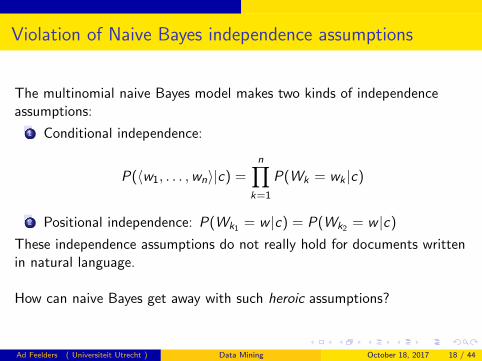
Violation of Naive Bayes independence assumptions
The multinomial naive Bayes model makes two kinds of independenceassumptions:
1 Conditional independence:
P(〈w1, . . . ,wn〉|c) =n∏
k=1
P(Wk = wk |c)
2 Positional independence: P(Wk1 = w |c) = P(Wk2 = w |c)
These independence assumptions do not really hold for documents writtenin natural language.
How can naive Bayes get away with such heroic assumptions?
Ad Feelders ( Universiteit Utrecht ) Data Mining October 18, 2017 18 / 44
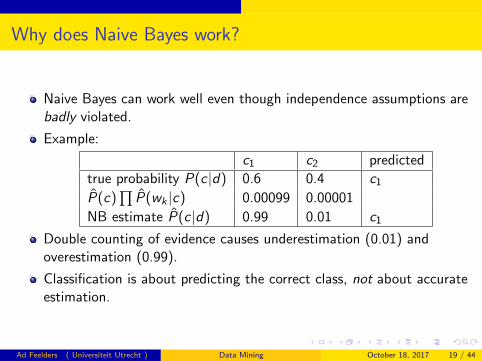
Why does Naive Bayes work?
Naive Bayes can work well even though independence assumptions arebadly violated.
Example:
c1 c2 predicted
true probability P(c |d) 0.6 0.4 c1P(c)
∏P(wk |c) 0.00099 0.00001
NB estimate P(c |d) 0.99 0.01 c1
Double counting of evidence causes underestimation (0.01) andoverestimation (0.99).
Classification is about predicting the correct class, not about accurateestimation.
Ad Feelders ( Universiteit Utrecht ) Data Mining October 18, 2017 19 / 44
Naive Bayes is not so naive
Probability estimates may be way off, but that doesn’t have to hurtclassification performance (much).
Requires the estimation of relatively few parameters, which may bebeneficial if you have a small training set.
Fast, low storage requirements
Ad Feelders ( Universiteit Utrecht ) Data Mining October 18, 2017 20 / 44
Feature Selection
The vocabulary of a training corpus may be huge, but not all words will begood class predictors.
How can we reduce the number of features?
Feature utility measures:
Frequency – select the most frequent terms.Mutual information – select the terms that have the highest mutualinformation with the class label.Chi-square test of independence between term and class label.
Sort features by utility and select top k.
Can we miss good sets of features this way?
Ad Feelders ( Universiteit Utrecht ) Data Mining October 18, 2017 21 / 44
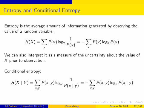
Entropy and Conditional Entropy
Entropy is the average amount of information generated by observing thevalue of a random variable:
H(X ) =∑
x
P(x) log21
P(x)= −
∑
x
P(x) log2 P(x)
We can also interpret it as a measure of the uncertainty about the value ofX prior to observation.
Conditional entropy:
H(X | Y ) =∑
x ,y
P(x , y) log21
P(x | y)= −
∑
x ,y
P(x , y) log2 P(x | y)
Ad Feelders ( Universiteit Utrecht ) Data Mining October 18, 2017 22 / 44
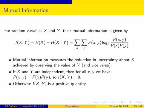
Mutual Information
For random variables X and Y , their mutual information is given by
I (X ;Y ) = H(X )− H(X | Y ) =∑
x
∑
y
P(x , y) log2P(x , y)
P(x)P(y)
Mutual information measures the reduction in uncertainty about Xachieved by observing the value of Y (and vice versa).
If X and Y are independent, then for all x , y we haveP(x , y) = P(x)P(y), so I (X ,Y ) = 0.
Otherwise I (X ;Y ) is a positive quantity.
Ad Feelders ( Universiteit Utrecht ) Data Mining October 18, 2017 23 / 44
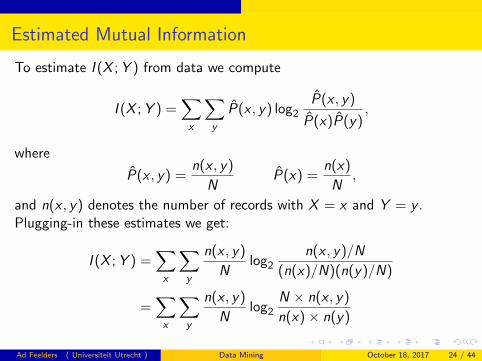
Estimated Mutual Information
To estimate I (X ;Y ) from data we compute
I (X ;Y ) =∑
x
∑
y
P(x , y) log2P(x , y)
P(x)P(y),
where
P(x , y) =n(x , y)
NP(x) =
n(x)
N,
and n(x , y) denotes the number of records with X = x and Y = y .Plugging-in these estimates we get:
I (X ;Y ) =∑
x
∑
y
n(x , y)
Nlog2
n(x , y)/N
(n(x)/N)(n(y)/N)
=∑
x
∑
y
n(x , y)
Nlog2
N × n(x , y)
n(x)× n(y)
Ad Feelders ( Universiteit Utrecht ) Data Mining October 18, 2017 24 / 44
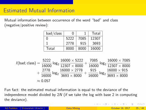
Estimated Mutual Information
Mutual information between occurrence of the word “bad” and class(negative/positive review):
bad/class 0 1 Total
0 5222 7085 123071 2778 915 3693
Total 8000 8000 16000
I (bad; class) =5222
16000log2
16000× 5222
12307× 8000+
7085
16000log2
16000× 7085
12307× 8000
+2778
16000log2
16000× 2778
3693× 8000+
915
16000log2
16000× 915
3693× 8000
≈ 0.057
Fun fact: the estimated mutual information is equal to the deviance of theindependence model divided by 2N (if we take the log with base 2 in computingthe deviance).
Ad Feelders ( Universiteit Utrecht ) Data Mining October 18, 2017 25 / 44
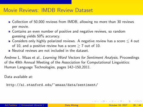
Movie Reviews: IMDB Review Dataset
Collection of 50,000 reviews from IMDB, allowing no more than 30 reviewsper movie.Contains an even number of positive and negative reviews, so randomguessing yields 50% accuracy.Considers only highly polarized reviews. A negative review has a score ≤ 4 outof 10, and a positive review has a score ≥ 7 out of 10.Neutral reviews are not included in the dataset.
Andrew L. Maas et al., Learning Word Vectors for Sentiment Analysis, Proceedingsof the 49th Annual Meeting of the Association for Computational Linguistics:Human Language Technologies, pages 142–150,2011.
Data available at:
http://ai.stanford.edu/~amaas/data/sentiment/
Ad Feelders ( Universiteit Utrecht ) Data Mining October 18, 2017 26 / 44

Analysis of Movie Reviews in R
# load the tm package
> library(tm)
# Read in the data using UTF-8 encoding
> reviews.neg <- Corpus(DirSource("D:/MovieReviews/train/neg",
encoding="UTF-8"))
> reviews.pos <- Corpus(DirSource("D:/MovieReviews/train/pos",
encoding="UTF-8"))
# Join negative and positive reviews into a single Corpus
> reviews.all <- c(reviews.neg,reviews.pos)
# create label vector (0=negative, 1=positive)
> labels <- c(rep(0,12500),rep(1,12500))
> reviews.all
<<VCorpus>>
Metadata: corpus specific: 0, document level (indexed): 0
Content: documents: 25000
Ad Feelders ( Universiteit Utrecht ) Data Mining October 18, 2017 27 / 44

Analysis of Movie Reviews
The first review before pre-processing:
> as.character(reviews.all[[1]])
[1] "Story of a man who has unnatural feelings for a pig.
Starts out with a opening scene that is a terrific example
of absurd comedy. A formal orchestra audience is turned into
an insane, violent mob by the crazy chantings of it’s singers.
Unfortunately it stays absurd the WHOLE time with no
general narrative eventually making it just too off putting.
Even those from the era should be turned off.
The cryptic dialogue would make Shakespeare seem easy to a
third grader. On a technical level it’s better than you might
think with some good cinematography by future great Vilmos Zsigmond.
Future stars Sally Kirkland and Frederic Forrest can be seen briefly."
Ad Feelders ( Universiteit Utrecht ) Data Mining October 18, 2017 28 / 44
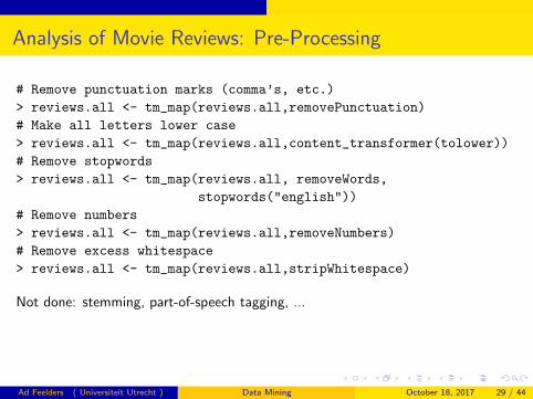
Analysis of Movie Reviews: Pre-Processing
# Remove punctuation marks (comma’s, etc.)
> reviews.all <- tm_map(reviews.all,removePunctuation)
# Make all letters lower case
> reviews.all <- tm_map(reviews.all,content_transformer(tolower))
# Remove stopwords
> reviews.all <- tm_map(reviews.all, removeWords,
stopwords("english"))
# Remove numbers
> reviews.all <- tm_map(reviews.all,removeNumbers)
# Remove excess whitespace
> reviews.all <- tm_map(reviews.all,stripWhitespace)
Not done: stemming, part-of-speech tagging, ...
Ad Feelders ( Universiteit Utrecht ) Data Mining October 18, 2017 29 / 44
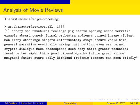
Analysis of Movie Reviews
The first review after pre-processing:
> as.character(reviews.all[[1]])
[1] "story man unnatural feelings pig starts opening scene terrific
example absurd comedy formal orchestra audience turned insane violent
mob crazy chantings singers unfortunately stays absurd whole time
general narrative eventually making just putting even era turned
cryptic dialogue make shakespeare seem easy third grader technical
level better might think good cinematography future great vilmos
zsigmond future stars sally kirkland frederic forrest can seen briefly"
Ad Feelders ( Universiteit Utrecht ) Data Mining October 18, 2017 30 / 44
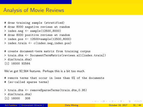
Analysis of Movie Reviews
# draw training sample (stratified)
# draw 8000 negative reviews at random
> index.neg <- sample(12500,8000)
# draw 8000 positive reviews at random
> index.pos <- 12500+sample(12500,8000)
> index.train <- c(index.neg,index.pos)
# create document-term matrix from training corpus
> train.dtm <- DocumentTermMatrix(reviews.all[index.train])
> dim(train.dtm)
[1] 16000 92564
We’ve got 92,564 features. Perhaps this is a bit too much.
# remove terms that occur in less than 5% of the documents
# (so-called sparse terms)
> train.dtm <- removeSparseTerms(train.dtm,0.95)
> dim(train.dtm)
[1] 16000 308
Ad Feelders ( Universiteit Utrecht ) Data Mining October 18, 2017 31 / 44
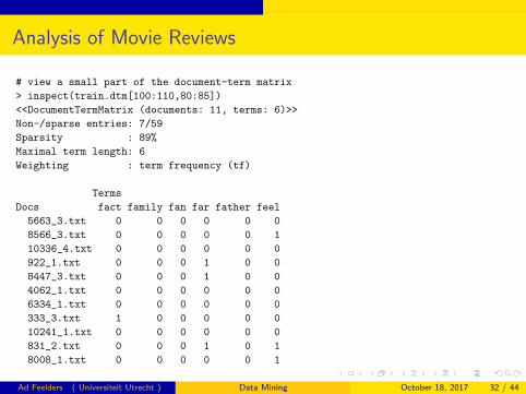
Analysis of Movie Reviews
# view a small part of the document-term matrix
> inspect(train.dtm[100:110,80:85])
<<DocumentTermMatrix (documents: 11, terms: 6)>>
Non-/sparse entries: 7/59
Sparsity : 89%
Maximal term length: 6
Weighting : term frequency (tf)
Terms
Docs fact family fan far father feel
5663_3.txt 0 0 0 0 0 0
8566_3.txt 0 0 0 0 0 1
10336_4.txt 0 0 0 0 0 0
922_1.txt 0 0 0 1 0 0
8447_3.txt 0 0 0 1 0 0
4062_1.txt 0 0 0 0 0 0
6334_1.txt 0 0 0 0 0 0
333_3.txt 1 0 0 0 0 0
10241_1.txt 0 0 0 0 0 0
831_2.txt 0 0 0 1 0 1
8008_1.txt 0 0 0 0 0 1
Ad Feelders ( Universiteit Utrecht ) Data Mining October 18, 2017 32 / 44
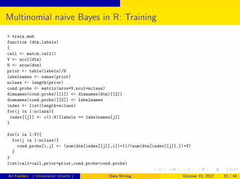
Multinomial naive Bayes in R: Training
> train.mnb
function (dtm,labels)
{
call <- match.call()
V <- ncol(dtm)
N <- nrow(dtm)
prior <- table(labels)/N
labelnames <- names(prior)
nclass <- length(prior)
cond.probs <- matrix(nrow=V,ncol=nclass)
dimnames(cond.probs)[[1]] <- dimnames(dtm)[[2]]
dimnames(cond.probs)[[2]] <- labelnames
index <- list(length=nclass)
for(j in 1:nclass){
index[[j]] <- c(1:N)[labels == labelnames[j]]
}
for(i in 1:V){
for(j in 1:nclass){
cond.probs[i,j] <- (sum(dtm[index[[j]],i])+1)/(sum(dtm[index[[j]],])+V)
}
}
list(call=call,prior=prior,cond.probs=cond.probs)
Ad Feelders ( Universiteit Utrecht ) Data Mining October 18, 2017 33 / 44
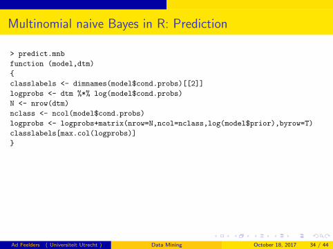
Multinomial naive Bayes in R: Prediction
> predict.mnb
function (model,dtm)
{
classlabels <- dimnames(model$cond.probs)[[2]]
logprobs <- dtm %*% log(model$cond.probs)
N <- nrow(dtm)
nclass <- ncol(model$cond.probs)
logprobs <- logprobs+matrix(nrow=N,ncol=nclass,log(model$prior),byrow=T)
classlabels[max.col(logprobs)]
}
Ad Feelders ( Universiteit Utrecht ) Data Mining October 18, 2017 34 / 44
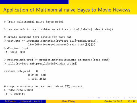
Application of Multinomial naive Bayes to Movie Reviews
# Train multinomial naive Bayes model
> reviews.mnb <- train.mnb(as.matrix(train.dtm),labels[index.train])
# create document term matrix for test set
> test.dtm <- DocumentTermMatrix(reviews.all[-index.train],
list(dictionary=dimnames(train.dtm)[[2]]))
> dim(test.dtm)
[1] 9000 308
> reviews.mnb.pred <- predict.mnb(reviews.mnb,as.matrix(test.dtm))
> table(reviews.mnb.pred,labels[-index.train])
reviews.mnb.pred 0 1
0 3459 848
1 1041 3652
# compute accuracy on test set: about 79% correct
> (3459+3652)/9000
[1] 0.7901111
Ad Feelders ( Universiteit Utrecht ) Data Mining October 18, 2017 35 / 44
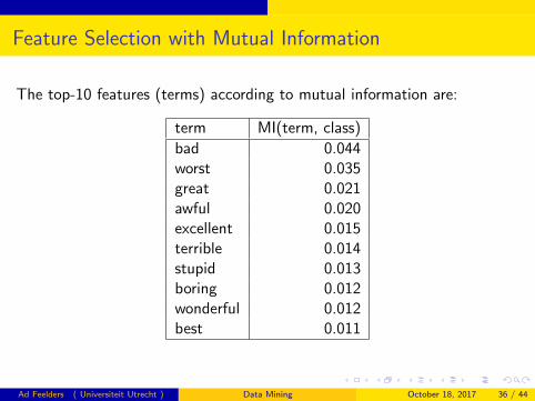
Feature Selection with Mutual Information
The top-10 features (terms) according to mutual information are:
term MI(term, class)
bad 0.044worst 0.035great 0.021awful 0.020excellent 0.015terrible 0.014stupid 0.013boring 0.012wonderful 0.012best 0.011
Ad Feelders ( Universiteit Utrecht ) Data Mining October 18, 2017 36 / 44
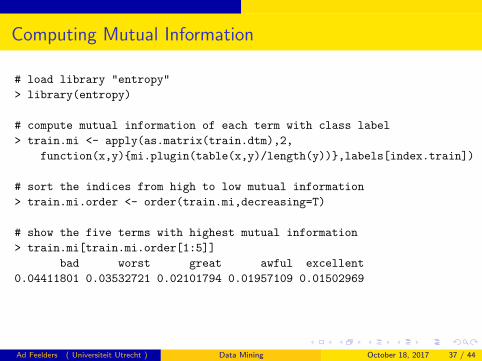
Computing Mutual Information
# load library "entropy"
> library(entropy)
# compute mutual information of each term with class label
> train.mi <- apply(as.matrix(train.dtm),2,
function(x,y){mi.plugin(table(x,y)/length(y))},labels[index.train])
# sort the indices from high to low mutual information
> train.mi.order <- order(train.mi,decreasing=T)
# show the five terms with highest mutual information
> train.mi[train.mi.order[1:5]]
bad worst great awful excellent
0.04411801 0.03532721 0.02101794 0.01957109 0.01502969
Ad Feelders ( Universiteit Utrecht ) Data Mining October 18, 2017 37 / 44
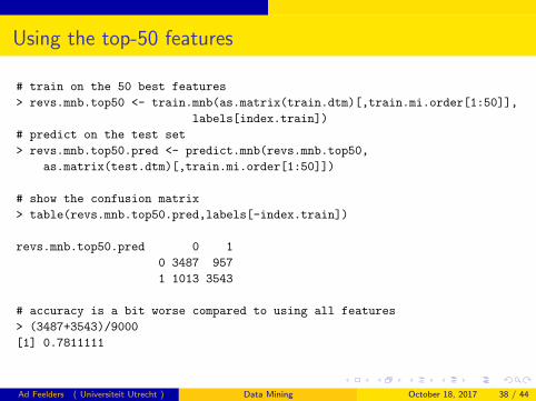
Using the top-50 features
# train on the 50 best features
> revs.mnb.top50 <- train.mnb(as.matrix(train.dtm)[,train.mi.order[1:50]],
labels[index.train])
# predict on the test set
> revs.mnb.top50.pred <- predict.mnb(revs.mnb.top50,
as.matrix(test.dtm)[,train.mi.order[1:50]])
# show the confusion matrix
> table(revs.mnb.top50.pred,labels[-index.train])
revs.mnb.top50.pred 0 1
0 3487 957
1 1013 3543
# accuracy is a bit worse compared to using all features
> (3487+3543)/9000
[1] 0.7811111
Ad Feelders ( Universiteit Utrecht ) Data Mining October 18, 2017 38 / 44
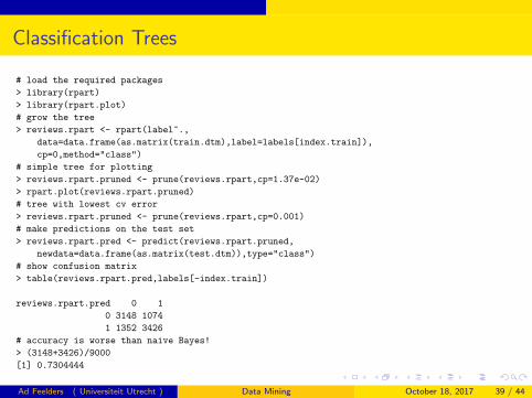
Classification Trees
# load the required packages
> library(rpart)
> library(rpart.plot)
# grow the tree
> reviews.rpart <- rpart(label~.,
data=data.frame(as.matrix(train.dtm),label=labels[index.train]),
cp=0,method="class")
# simple tree for plotting
> reviews.rpart.pruned <- prune(reviews.rpart,cp=1.37e-02)
> rpart.plot(reviews.rpart.pruned)
# tree with lowest cv error
> reviews.rpart.pruned <- prune(reviews.rpart,cp=0.001)
# make predictions on the test set
> reviews.rpart.pred <- predict(reviews.rpart.pruned,
newdata=data.frame(as.matrix(test.dtm)),type="class")
# show confusion matrix
> table(reviews.rpart.pred,labels[-index.train])
reviews.rpart.pred 0 1
0 3148 1074
1 1352 3426
# accuracy is worse than naive Bayes!
> (3148+3426)/9000
[1] 0.7304444
Ad Feelders ( Universiteit Utrecht ) Data Mining October 18, 2017 39 / 44
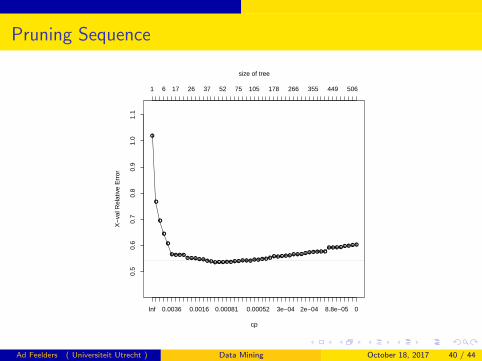
Pruning Sequence
●
●
●
●
●
● ● ● ●● ● ● ● ● ● ● ● ● ● ● ● ● ● ● ● ● ● ● ● ● ● ● ● ● ● ● ● ● ● ● ● ● ● ● ●
● ● ● ● ● ● ● ●
cp
X−
val R
elat
ive
Err
or
0.5
0.6
0.7
0.8
0.9
1.0
1.1
Inf 0.0036 0.0016 0.00081 0.00052 3e−04 2e−04 8.8e−05 0
1 6 17 26 37 52 75 105 178 266 355 449 506
size of tree
Ad Feelders ( Universiteit Utrecht ) Data Mining October 18, 2017 40 / 44
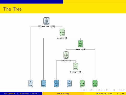
The Tree
bad >= 0.5
worst >= 0.5
great < 0.5
awful >= 0.5
boring >= 0.5
00.50
100%
00.2523%
10.5877%
00.135%
10.6172%
10.5553%
00.122%
10.5751%
00.242%
10.5949%
10.7519%
yes no
Ad Feelders ( Universiteit Utrecht ) Data Mining October 18, 2017 41 / 44
The Second Assignment: Text Classification
Text Classification for the Detection of Opinion Spam.
We analyze fake and genuine hotel reviews.
The genuine reviews have been collected from several popular onlinereview communities.
The fake reviews have been obtained from Mechanical Turk.
There are 400 reviews in each of the categories: positive truthful,positive deceptive, negative truthful, negative deceptive.
We will focus on the negative reviews and try to discriminate betweentruthful and deceptive reviews.
Hence, the total number of reviews in our data set is 800.
Ad Feelders ( Universiteit Utrecht ) Data Mining October 18, 2017 42 / 44

The Second Assignment: Text Classification
Analyse the data with:
1 Naive Bayes (generative linear classifier),
2 Regularized logistic regression (discriminative linear classifier),
3 Classification trees, (flexible classifier) and
4 Random forests (flexible classifier).
Ad Feelders ( Universiteit Utrecht ) Data Mining October 18, 2017 43 / 44
The Second Assignment: Text Classification
This is a data analysis assignment, not a programming assignment.
You will need to program a little to be able to perform theexperiments.
You only need to hand in a report of your analysis.
We recommend and support certain R packages (such as tm), but youare free to use whatever tools you want.
For possibly relevant R packages, have a look at:
https://cran.r-project.org/web/views/NaturalLanguageProcessing.html
The report should describe the analysis you performed in such a waythat the reader would be able reproduce it.
Ad Feelders ( Universiteit Utrecht ) Data Mining October 18, 2017 44 / 44