Embed Size (px)
Citation preview
Data Integration for Querying GeospatialSources�
Isabel F. Cruz and Huiyong Xiao
Department of Computer ScienceUniversity of Illinois at Chicago{ifc | hxiao}@cs.uic.edu
Abstract. Geospatial data management is fundamental for many ap-plications including land use planning and transportation and is criticalin emergency management. However, geospatial data are distributed,complex, and heterogeneous due to being independently developed byvarious levels of government and the private sector. Until now, the for-mulation of expressive queries on geospatial data, which contrast withsimple keyword-based queries, requires both user expertise and a greatdeal of manual intervention to determine the mappings between conceptsin potentially dozens of data sources.In this paper, we describe an ontology-based approach to the problem ofdata integration, specifically focusing on the issue of query processing in aheterogeneous setting. Our contributions include a mechanism for meta-data representation, an ontology alignment process, and a sound queryrewriting algorithm for answering queries across distributed geospatialdata sources. We demonstrate the practical impact of our approach inland use applications, which are exemplary of the extreme heterogeneityof data. We are leveraging current and emerging Semantic Web standardsand tools for modeling, storing, and processing data. Our contributionto geospatial data integration is significant because new data sources canbe added with relatively little effort, thus allowing for data manipulationand querying to extend seamlessly to the new data sources.
1 Introduction
Years of autonomic and uncoordinated development of classification schemesby government organizations and the private sector pose enormous challengesin integrating geospatial data. In this paper, our focus is on the integration ofgeospatial data that is created by the different counties and municipalities in thestate of Wisconsin and stored locally by the counties and municipalities. Amongthe available geospatial data, we have concentrated on land use data. We haveworked with the Wisconsin local government within the scope of WLIS (Wiscon-sin Land Information System) and the National Science Foundation under theirDigital Government and Information Integration programs. Data heterogeneity� This research was partially supported by the National Science Foundation under
Awards ITR IIS-0326284 and IIS-0513553.
2 Isabel F. Cruz and Huiyong Xiao
in the land use data domain has been hindering the cooperation among the localgovernments to achieve comprehensive land use planning across the borders ofthe different jurisdictions [33].
We propose an ontology-based approach to enable integration and interoper-ability of the local data sources. In our work we deal with two kinds of ontologies:an axiomatized set of concepts and relationship types and a taxonomy of entities[17]. We call the first kind schema-like ontologies, because they are associatedwith the structure or schema of the local sources. The second kind model theentities (instance names) that describe land usage (for example, agricultural,commercial, or residential), where the only type of relationship is that of sub-concept (or subclass) (for example, single family residences and multiple familyresidences are two subconcepts of residential), and are called taxonomy-like on-tologies in our discussion.
The ontologies that we use to represent the structure of the local data sources,which we call local ontologies, belong to the first type and can be obtained fromthe source schemas through a schema transformation process. The second typeof ontologies are the land use ontologies, which are part of the local ontologies;they represent land use taxonomies that classify land parcels in the local datasources according to their usage. In addition, our approach uses a global ordomain ontology that models the domain associated with the task at hand andenables mediation across the local data sources. The global ontology contains aglobal land use ontology that describes the land use domain.
The key to our approach lies in establishing mappings between the conceptsof the global ontology and the concepts of the local ontologies, a process calledalignment. Using those mappings, a single query can then be expressed in termsof the concepts of the global ontology (or of a local ontology) and be automati-cally rewritten and posed against the other ontologies. We focus on database-stylequeries as opposed to simpler and less expressive keyword-based queries.
Query processing can be performed in two ways: global-to-local and local-to-local. In the former case, we rewrite a query posed on the global ontology intosubqueries over the local sources (the global ontology acts as a uniform queryinterface of the integration system). In the latter case, we translate a query posedon a geospatial source to a query on any other geospatial source.
In this paper, we consider the alignment process of the local land use ontologywith the global land use ontology and propose an ontology alignment algorithmbased on a set of deduction rules, which can be performed automatically whencertain pre-conditions are established. We propose a sound query rewriting al-gorithm. The algorithm can compute a contained rewriting of a query in bothglobal-to-local and local-to-local querying. Query containment ensures that allthe answers retrieved by executing the rewriting are a subset of the answer tothe original query, thus guaranteeing precise query answering across distributeddata sources [23].
The rest of the paper is organized as follows. The data heterogeneity issues inland use management are discussed in Section 2. The ontology creation processis described in Section 3. In Section 4, we focus on an automatic algorithm for
Data Integration for Querying Geospatial Sources 3
ontology alignment. Query answering is presented in Section 5. In Section 6, wedescribe briefly the user interfaces that support ontology alignment and queryprocessing. We summarize related work in Section 7. Finally, we draw conclusionsand outline directions for future research in Section 8.
2 Data Heterogeneities
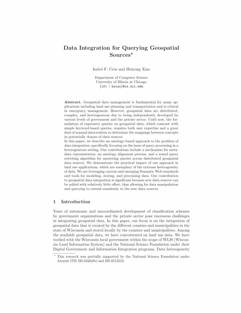
In this section, we describe in detail the kinds of heterogeneities that we en-counter when integrating data from the local geospatial sources. In these sources,data is stored in XML format. Figure 1 shows two fragments of land parcel data,including their DTD (on the left-hand side) and an XML fragment (on the right-hand side), which respectively exist in the local systems of Eau Claire Countyand Madison County. As we can observe, even though the local XML sourcespresent different structures and naming conventions, they share a common do-main with closely related meanings (or semantics), thus being ideal candidatesfor an integration system.
The previous examples display syntactic homogeneity in that they both useXML but have different structures, therefore displaying schematic heterogeneity.They may also encode their instances or values in different ways, thus displayingsemantic heterogeneity, in the sense that the same values may represent differentmeanings and that different values may have the same meaning [32]. Our discus-sion elaborates further on both kinds of heterogeneities. In the example shownin Figure 1, we see that the two source schemas overlap on most elements andboth have the same nesting depth. However, the elements of the land use codesare represented differently in the two schemas: the schema S1 uses four elements(broad, lu1, lu2, and lu3), whereas S2 uses a single element (land use). Fur-thermore, the values of such land use codes (in the XML instances) are encodedin different ways, namely characters for S1 and numbers for S2.
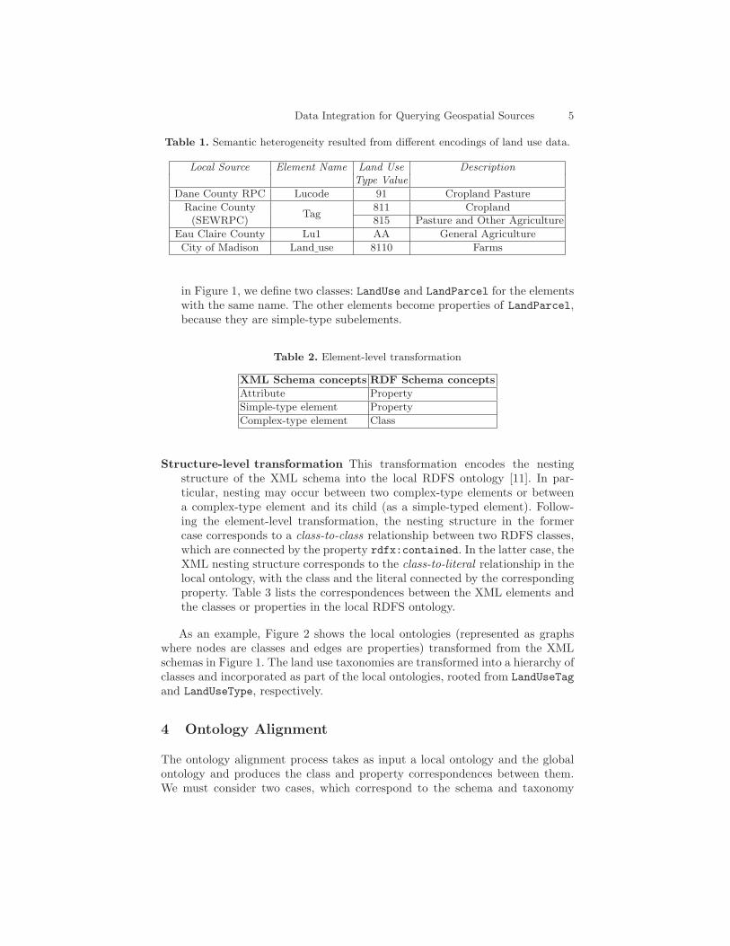
Land use codes in WLIS stand for land use types (or categories) and include,for example, agriculture, commerce, industry, institutions and residences. Besidesusing different names in different local source schemas, such land use codes havedifferent classification schemes associated with them, thus resulting in semanticheterogeneities across the local source schemas. This is illustrated by Table 1,where there are four element names (Lucode, Tag, Lu1 and Land use) from fourdifferent classification schemas. The descriptions in the table show that differentvalues represent closely related land use types.
In our approach, a local ontology is generated for each local XML sourcethat represents its schema. In addition, a global or domain ontology is definedto act as an integrated view and a uniform access interface to the distributeddata sources. Every local ontology is mapped to this global ontology, by estab-lishing the correspondences of their elements and attributes, which results in analignment on the local names. In addition to this schema level reconciliation, itis also necessary to have a global land use taxonomy, to which the local landuse taxonomies are mapped, so as to achieve a common understanding of the se-
4 Isabel F. Cruz and Huiyong Xiao
<?xml encoding="ISO-8859-1"?> <LandUse><!ELEMENT LandUse (LandParcel)> <LandParcel><!ELEMENT LandParcel (AREA, BROAD, LU1, <AREA>1704995.587470</AREA>
LU2, LU3, ..., JurisType, JurisName)> <BROAD>A</BROAD><!ELEMENT AREA (#PCDATA)> <LU1>AF</LU1><!ELEMENT BROAD (#PCDATA)> ......
<!ELEMENT LU1 (#PCDATA)> <JurisType>County</JurisType>...... <JurisName>EauClaire</JurisName><!ELEMENT JurisType (#PCDATA)> </LandParcel><!ELEMENT JurisName (#PCDATA)> ......
</LandUse>
a) Local XML data source S1 of Eau Claire County.
<?xml encoding="ISO-8859-1"?> <LandUse><!ELEMENT LandUse (LandParcel)> <LandParcel><!ELEMENT LandParcel (AREA, LAND USE, <AREA>1007908.5</AREA>
PARCEL ID, ..., JurisType, JurisName)> <LAND USE>9100</LAND USE><!ELEMENT AREA (#PCDATA)> <PARCEL ID>246710</PARCEL ID><!ELEMENT LAND USE (#PCDATA)> ......
<!ELEMENT PARCEL ID (#PCDATA)> <JurisType>County</JurisType>...... <JurisName>Madison</JurisName><!ELEMENT JurisType (#PCDATA)> </LandParcel><!ELEMENT JurisName (#PCDATA)> ......
</LandUse>
b) Local XML data source S2 of the City of Madison.
Fig. 1. Local XML land use data sources. In the data source S1, BROAD and LU1 definethe land use code, with BROAD as the first level and LU1 as a child level of BROAD. Inthe data source S2, LAND USE specifies the land use code. In both sources, the elementsJurisType and JurisName contain the jurisdiction type and name, respectively.
mantics of the land use codes in the local sources. All ontologies are representedusing RDF and RDFS.
3 Ontology Creation
The first step of the integration of XML geospatial data sources is the trans-formation from the XML source schema and data to an RDFS ontology and toRDF data. This transformation encompasses the following steps:
Element-level transformation This transformation defines the basic classesand properties of the local RDFS ontology according to the transformationcorrespondences shown in Table 2, with the structural relationships betweenthe elements not being considered for the time being. No new RDF metadataneed be defined here because rdfs:Class and rdfs:Property are sufficientto express classes and properties. For instance, to transform the DTD of S1
Data Integration for Querying Geospatial Sources 5
Table 1. Semantic heterogeneity resulted from different encodings of land use data.
Local Source Element Name Land Use DescriptionType Value
Dane County RPC Lucode 91 Cropland Pasture
Racine CountyTag
811 Cropland(SEWRPC) 815 Pasture and Other Agriculture
Eau Claire County Lu1 AA General Agriculture
City of Madison Land use 8110 Farms
in Figure 1, we define two classes: LandUse and LandParcel for the elementswith the same name. The other elements become properties of LandParcel,because they are simple-type subelements.
Table 2. Element-level transformation
XML Schema concepts RDF Schema concepts
Attribute Property
Simple-type element Property
Complex-type element Class
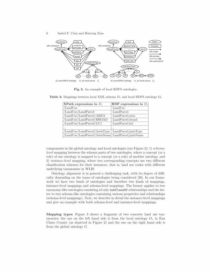
Structure-level transformation This transformation encodes the nestingstructure of the XML schema into the local RDFS ontology [11]. In par-ticular, nesting may occur between two complex-type elements or betweena complex-type element and its child (as a simple-typed element). Follow-ing the element-level transformation, the nesting structure in the formercase corresponds to a class-to-class relationship between two RDFS classes,which are connected by the property rdfx:contained. In the latter case, theXML nesting structure corresponds to the class-to-literal relationship in thelocal ontology, with the class and the literal connected by the correspondingproperty. Table 3 lists the correspondences between the XML elements andthe classes or properties in the local RDFS ontology.
As an example, Figure 2 shows the local ontologies (represented as graphswhere nodes are classes and edges are properties) transformed from the XMLschemas in Figure 1. The land use taxonomies are transformed into a hierarchy ofclasses and incorporated as part of the local ontologies, rooted from LandUseTagand LandUseType, respectively.
4 Ontology Alignment
The ontology alignment process takes as input a local ontology and the globalontology and produces the class and property correspondences between them.We must consider two cases, which correspond to the schema and taxonomy
6 Isabel F. Cruz and Huiyong Xiao
LandUse
LandParcel
rdfx:contained
Literal
rdfs:domain
rdfs:range
area
broad
lu1
jurisType
jurisName
Property
Class
LandUseTagrdfs:subClassOf
A R. . .
. . .
lu2
lu3
LandUse
LandParcel
rdfx:contained
Literal
area
Land_use
jurisType
jurisName
LandUseType
. . .
. . .
AA AD. . . RB RC. . .
parcel_id
1 8
11 12 19 81 8100810
a) Local RDFS ontology O1 for local source S1 b) Local RDFS ontology O2 for local source S2
Fig. 2. An example of local RDFS ontologies.
Table 3. Mappings between local XML schema D1 and local RDFS ontology O1
XPath expressions in D1 RDF expressions in O1
/LandUse LandUse
/LandUse/LandParcel LandParcel
/LandUse/LandParcel/AREA LandParcel.area
/LandUse/LandParcel/BROAD LandParcel.broad
/LandUse/LandParcel/LU1 LandParcel.lu1
... ...
/LandUse/LandParcel/JurisType LandParcel.jurisType
/LandUse/LandParcel/JurisName LandParcel.jurisName
components in the global ontology and local ontologies (see Figure 2): 1) schema-level mapping between the schema parts of two ontologies, where a concept (or arole) of one ontology is mapped to a concept (or a role) of another ontology, and2) instance-level mapping, where two corresponding concepts use two differentclassification schemes for their instances, that is, land use codes with differentunderlying taxonomies in WLIS.
Ontology alignment is in general a challenging task, with its degree of diffi-culty depending on the types of ontologies being considered [30]. In our frame-work we have two kinds of ontologies and therefore two kinds of mappings,instance-level mappings and schema-level mappings. The former applies to twotaxonomy-like ontologies consisting of only subClassOf relationships and the lat-ter to two schema-like ontologies containing various properties and relationships(schema-level mappings). Next, we describe in detail the instance-level mappingsand give an example with both schema-level and instance-level mappings.
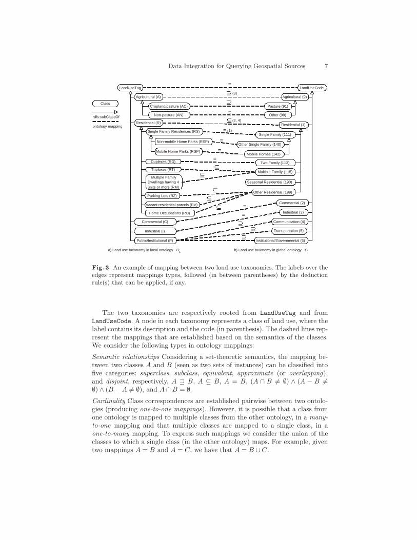
Mapping types Figure 3 shows a fragment of two concrete land use tax-onomies: the one on the left hand side is from the local ontology O1 in EauClaire County (as depicted in Figure 2) and the one on the right hand side isfrom the global ontology G.
Data Integration for Querying Geospatial Sources 7
rdfs:subClassOf
Class
ontology mapping
LandUseTag
Agricultural (A)
Residential (R)
Commercial (C)
Industrial (I)
Public/Institutional (P)
Single Family Residences (RS)
Mobile Home Parks (RSP)
LandUseCode
Agricultural (9)
Residential (1)
Transportation (5)
Industrial (3)
Single Family (111)
Two Family (113)
Multiple Family (115)
Other Single Family (140)
Mobile Homes (142)
Seasonal Residential (190)Multiple Family
Dwellings having 4units or more (RM)
Home Occupations (RO)
Vacant residential parcels (RV)
Parking Lots (RZ)
Communication (4)
Commercial (2)
Institutional/Governmental (6)
Non-mobile Home Parks (RSP)
Other Residential (199)
Duplexes (RD)
Triplexes (RT)
Cropland/pasture (AC)
Non-pasture (AN)
Pasture (91)
Other (99)
a) Land use taxonomy in local ontology O1
b) Land use taxonomy in global ontology G
=
=
= (1)
=
(2, 4)
=
=
=
(3)
=
Fig. 3. An example of mapping between two land use taxonomies. The labels over theedges represent mappings types, followed (in between parentheses) by the deductionrule(s) that can be applied, if any.
The two taxonomies are respectively rooted from LandUseTag and fromLandUseCode. A node in each taxonomy represents a class of land use, where thelabel contains its description and the code (in parenthesis). The dashed lines rep-resent the mappings that are established based on the semantics of the classes.We consider the following types in ontology mappings:
Semantic relationships Considering a set-theoretic semantics, the mapping be-tween two classes A and B (seen as two sets of instances) can be classified intofive categories: superclass, subclass, equivalent, approximate (or overlapping),and disjoint, respectively, A ⊇ B, A ⊆ B, A = B, (A ∩ B �= ∅) ∧ (A − B �=∅) ∧ (B −A �= ∅), and A ∩B = ∅.Cardinality Class correspondences are established pairwise between two ontolo-gies (producing one-to-one mappings). However, it is possible that a class fromone ontology is mapped to multiple classes from the other ontology, in a many-to-one mapping and that multiple classes are mapped to a single class, in aone-to-many mapping. To express such mappings we consider the union of theclasses to which a single class (in the other ontology) maps. For example, giventwo mappings A = B and A = C, we have that A = B ∪ C.
8 Isabel F. Cruz and Huiyong Xiao
Coverage We distinguish two types of mappings: fully covered and partially cov-ered. Let C and C ′ be two classes to be mapped, such that C1, ..., Cm are sub-classes of C, and C ′
1, ..., C′n are subclasses of C ′. We say that C (resp. C ′) is fully
covered if for each child Ci ∈ {C1, ..., Cm} (resp. for each child C ′j ∈ {C ′
1, ..., C′n})
there is a non-empty subset of {C ′1, ..., C
′n} to which Ci is mapped (respectively
there is a non-empty subset of {C1, ..., Cm} to which C ′j is mapped).
Deduction process In our approach, the ontology mapping process is per-formed using an inference process based on deduction rules. In the case that thededuction rules do not apply, then manual intervention by the user is needed.
This semi-automatic ontology mapping process follows two principles: (1)The deduction of the mapping between two nodes (from both taxonomies beingmapped) is determined by the mappings between their children. In other words,the mapping between two ontologies are performed in a level-wise fashion, drivenby the deduction rules that are defined based on the mapping semantics. (2) Theuser intervention is needed in two cases: when the mapping between two nodeshas insufficient information to determine its type (for example, when some ofthe children of one node have not been mapped) or when there is conflictinginformation (for example, that a node is both a superset and a subset of thecorresponding node).
We make the complete-partition assumption: for any class C in the taxon-omy, its subclasses C1, ..., Cn form a complete partition of the class, that is,C = C1 ∪ ... ∪ Cn. For instance, in the global taxonomy depicted in Figure 3,the two children Pasture(91) and Other(99) of the Agricultural(9) classform a complete partition of Agricultural(9), since Other(99) includes allagricultural lands that are not used for pasture.
We consider the following deduction rules:
Definition 1 (Deduction rules). Let C and C ′ be two fully covered classes,and C1, ..., Cm and C ′
1, ..., C′n be the subclasses of C and C ′, respectively. Then,
the mapping between C and C ′ can be obtained according to the following rules:
1) C = C ′, if for each Ci ∈ C, Ci is mapped to some k-element subset C ′′ of{C ′
1, ..., C′n} ( 1 ≤ k ≤ n′), such that Ci =
⋃kl=1 C
′′l .
2) C ⊆ C ′, if for each Ci ∈ C, Ci is mapped to some k-element subset C ′′ of{C ′
1, ..., C′n} ( 1 ≤ k ≤ n′), such that Ci =
⋃kl=1 C
′′l or Ci ⊆
⋃kl=1 C
′′l .
3) C ⊇ C ′, if for each Ci ∈ C, Ci is mapped to some k-element subset C ′′ of{C ′
1, ..., C′n} ( 1 ≤ k ≤ n′), such that Ci =
⋃kl=1 C
′′l or Ci ⊇
⋃kl=1 C
′′l .
The deduction rules in Definition 1 can be proved to be sound and completeby an induction on the set-theoretic semantics of each rule, under the complete-partition assumption and the assumption that the user-defined mappings aresemantically correct.
The above rules assume a full mapping between C and C ′. However, theystill hold for the case of a partial mapping, provided that we define the followingsupplemental rule: 4) Suppose that a class C is partially covered by C ′ and that
Data Integration for Querying Geospatial Sources 9
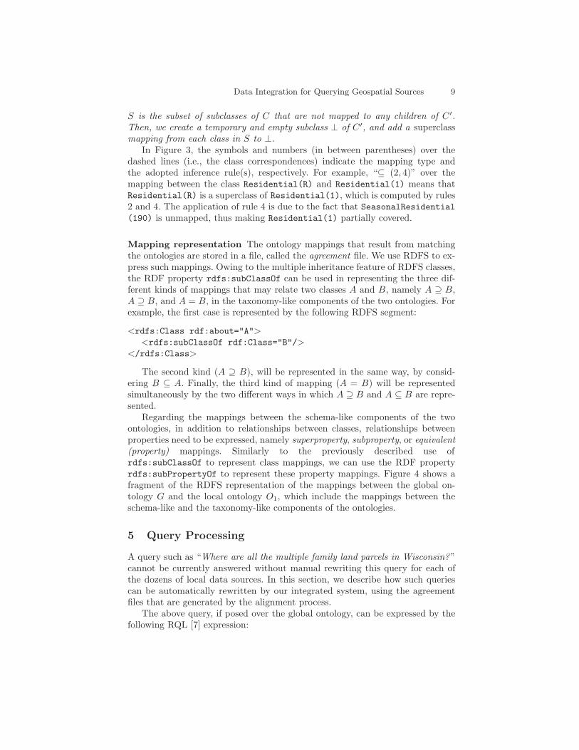
S is the subset of subclasses of C that are not mapped to any children of C ′.Then, we create a temporary and empty subclass ⊥ of C ′, and add a superclassmapping from each class in S to ⊥.
In Figure 3, the symbols and numbers (in between parentheses) over thedashed lines (i.e., the class correspondences) indicate the mapping type andthe adopted inference rule(s), respectively. For example, “⊆ (2, 4)” over themapping between the class Residential(R) and Residential(1) means thatResidential(R) is a superclass of Residential(1), which is computed by rules2 and 4. The application of rule 4 is due to the fact that SeasonalResidential(190) is unmapped, thus making Residential(1) partially covered.
Mapping representation The ontology mappings that result from matchingthe ontologies are stored in a file, called the agreement file. We use RDFS to ex-press such mappings. Owing to the multiple inheritance feature of RDFS classes,the RDF property rdfs:subClassOf can be used in representing the three dif-ferent kinds of mappings that may relate two classes A and B, namely A ⊇ B,A ⊇ B, and A = B, in the taxonomy-like components of the two ontologies. Forexample, the first case is represented by the following RDFS segment:
<rdfs:Class rdf:about="A"><rdfs:subClassOf rdf:Class="B"/>
</rdfs:Class>
The second kind (A ⊇ B), will be represented in the same way, by consid-ering B ⊆ A. Finally, the third kind of mapping (A = B) will be representedsimultaneously by the two different ways in which A ⊇ B and A ⊆ B are repre-sented.
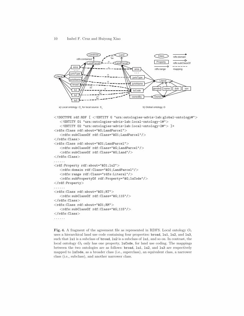
Regarding the mappings between the schema-like components of the twoontologies, in addition to relationships between classes, relationships betweenproperties need to be expressed, namely superproperty, subproperty, or equivalent(property) mappings. Similarly to the previously described use ofrdfs:subClassOf to represent class mappings, we can use the RDF propertyrdfs:subPropertyOf to represent these property mappings. Figure 4 shows afragment of the RDFS representation of the mappings between the global on-tology G and the local ontology O1, which include the mappings between theschema-like and the taxonomy-like components of the ontologies.
5 Query Processing
A query such as “Where are all the multiple family land parcels in Wisconsin?”cannot be currently answered without manual rewriting this query for each ofthe dozens of local data sources. In this section, we describe how such queriescan be automatically rewritten by our integrated system, using the agreementfiles that are generated by the alignment process.
The above query, if posed over the global ontology, can be expressed by thefollowing RQL [7] expression:
10 Isabel F. Cruz and Huiyong Xiao
LandParcel
Literal
rdfs:domain
rdfs:range
jurisType
jurisName
luCode
ownedBy
Property
Class
rdfs:subClassOf
LandUse
LandParcel
rdfx:contained
Literal
area
broad
lu1
jurisType
jurisName
. . .
lu2
lu3
a) Local ontology O1 for local source S
1
area
Owner
name dob ssngender
. . .
Land
mapping
=
=
=
=
=
b) Global ontology G
<!DOCTYPE rdf:RDF [ <!ENTITY G "urn:ontologies-advis-lab:global-ontology#"><!ENTITY O1 "urn:ontologies-advis-lab:local-ontology-1#"><!ENTITY O2 "urn:ontologies-advis-lab:local-ontology-2#"> ]>
<rdfs:Class rdf:about="&G;LandParcel"><rdfs:subClassOf rdf:Class="&O1;LandParcel"/>
</rdfs:Class><rdfs:Class rdf:about="&O1;LandParcel">
<rdfs:subClassOf rdf:Class="&G;LandParcel"/><rdfs:subClassOf rdf:Class="&G;Land"/>
</rdfs:Class>......
<rdf:Property rdf:about="&O1;lu2"><rdfs:domain rdf:Class="&O1;LandParcel"/><rdfs:range rdf:Class="rdfs:Literal"/><rdfs:subPropertyOf rdf:Property="&G;luCode"/>
</rdf:Property>......
<rdfs:Class rdf:about="&O1;RT"><rdfs:subClassOf rdf:Class="&G;115"/>
</rdfs:Class><rdfs:Class rdf:about="&O1;RM">
<rdfs:subClassOf rdf:Class="&G;115"/></rdfs:Class>......
Fig. 4. A fragment of the agreement file as represented in RDFS. Local ontology O1
uses a hierarchical land use code containing four properties: broad, lu1, lu2, and lu3,such that lu1 is a subclass of broad, lu2 is a subclass of lu1, and so on. In contrast, thelocal ontology O2 only has one property, luCode, for land use coding. The mappingsbetween the two ontologies are as follows: broad, lu1, lu2, and lu3 are respectivelymapped to luCode, as a broader class (i.e., superclass), an equivalent class, a narrowerclass (i.e., subclass), and another narrower class.
Data Integration for Querying Geospatial Sources 11
SELECT a, b, cFROM {$x}xyCoordinates{a}, {$x}bounding{b}, {$x}jurisName{c},
{$x}state{d}, {$x}luCode{e}WHERE d = "Wisconsin" and e = "115"
In the FROM clause, we use basic schema path expressions composed of theproperty name (e.g., bounding) and data variables (e.g., $x) or class variables(e.g., a). The properties xyCoordinates and bounding stand for the geographi-cal coordinates and boundaries of the land parcel, respectively. The other prop-erties were already discussed and shown in Figures 1 and 4. In what follows, wefocus on a particular subset of RQL, namely conjunctive RQL (c-RQL), whichis of the following form: ans(x) :– R1(x1), ..., Rn(xn)., where x ⊆ x1 ∪ ... ∪ xn
are variables or constants, and Ri(xi) (i ∈ [1..n]) is either a class predicate C(x)or a property predicate P (x, y). As usual, ans(x) is the head of the query, de-noted headQ, and R1(x1), ..., Rn(xn) is the body of the query, denoted bodyQ.For instance, the RQL query on multiple family land parcels can be expressedin c-RQL as follows:
ans(a, b, c) :– xyCoordinates(x, a), bounding(x, b), jurisName(x, c),state(x, "Wisconsin"), luCode(x, "115").
Query processing across the whole system can be performed in two direc-tions: global-to-local and local-to-local. We propose a query rewriting algorithm,QueryRewriting, which can be used in both cases. Query rewriting can be seenas a function Q′ = f(Q,M), where Q is the query to be rewritten, called sourcequery, M is the set of ontology mappings, and Q′ is the resulting query, calledtarget query. The algorithm is shown in Figure 5.
In the global-to-local case, the source query Q is posed on the global ontologyG, M is the set of mappings from G to every local ontology O1, ..., On, and thetarget query Q′ is the union of multiple subqueries over O1, ..., On. In the local-to-local case, Q is a local query posed on a local ontology Oi (i ∈ [1..n]), M isthe set of mappings from Oi to one or more local ontologies Oj (j ∈ [1..n] andj �= i), and Q′ is the union of multiple subqueries over all Oj . In the latter case,M is, in fact, a set of compositions of the mappings from Oi to G with thosefrom G to Oj .
The QueryRewriting algorithm consists of four main steps: 1) source queryexpansion using the source ontology constraints, 2) schema-level mapping wherethe expanded source query is rewritten into an intermediate target query usingschema-level mappings, 3) intermediate target query expansion using the targetontology constraints, and 4) instance-level mapping where the expanded inter-mediate target query is rewritten using instance-level mappings to obtain thefinal target query. In what follows, we cover the overall query processing by de-scribing the three key components of the four main steps listed above: queryexpansion, schema-level mapping, and instance-level mapping. Finally, we dis-cuss some of our assumptions and prove the correctness of the query rewritingalgorithm.
12 Isabel F. Cruz and Huiyong Xiao
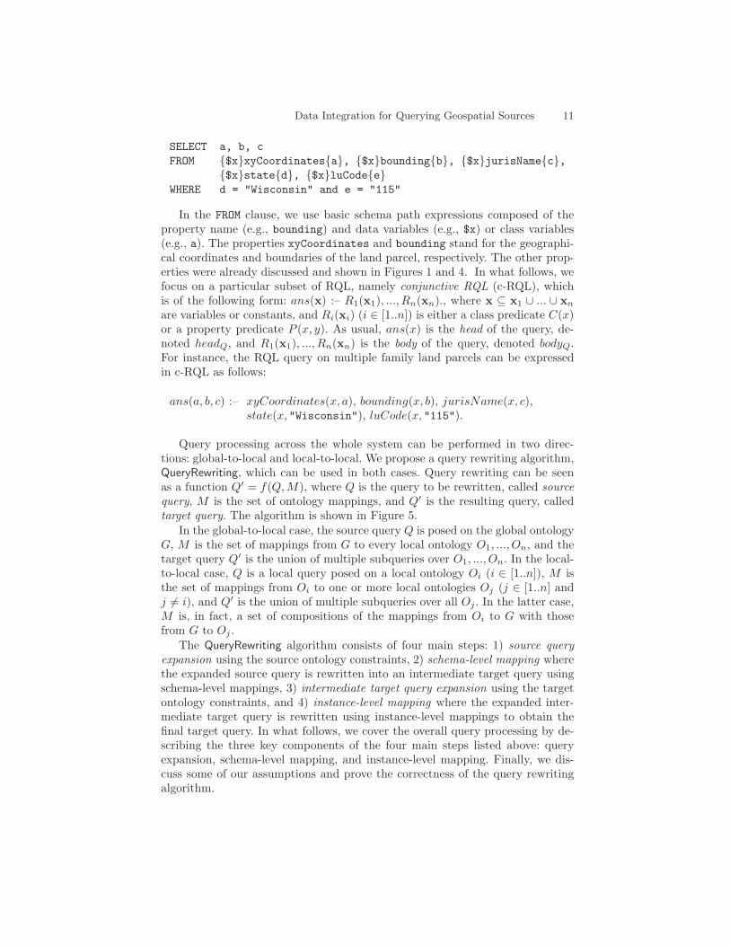
Algorithm QueryRewriting (Q, M)Input: a conjunctive query Q over ontology O; the mappings M betweenontologies O and O′.Output: a union Q of conjunctive queries Q′ over O′.1 headQ′ = headQ; bodyQ′ = null;2 Q∗ = QueryExpand(Q, Σ), where Σ is the set of constraints over O;3 Let φ be bodyQ∗ ;4 Let M1 be the part of schema-level mappings in M ;5 For each R(x) of φ6 For each ψ ∈M1
7 Let R′(x′) be the result of applying ψ on R(x);8 bodyQ′ = R′(x′) ∧ bodyQ′ ;9 Q′ = QueryExpand(Q′, Σ′), where Σ′ is the set of constraints over O′;10 Let M2 be the part of instance-level mappings in M ;11 Q = ConstantMapping(Q′, M2);12 Return Q;
Fig. 5. The QueryRewriting algorithm.
Query expansion In the above description of the QueryRewriting algorithm,both the source query Q and the intermediate target query Q′ are expandedusing the ontology constraints, respectively in Lines 2 and 9. This query ex-pansion process, as described by the QueryExpand function of Figure 6, usesthe strategy of applying the ontology constraints to “chase” the query, similarlyto the chase algorithm that is used in relational databases to compute depen-dency implications or optimize queries [1]. In relational databases, a databaseconstraint can be represented as a tgd (tuple generating dependency) in the form∀x∃y ϕ(x) → ψ(x,y), where ϕ and ψ are conjunctions of atoms. In an ontologysetting, we consider three kinds of constraints, namely, subclass, subproperty,and typing constraints, all of which can be represented as a tgd. Specifically, thetgd ∀x C1(x) → C2(x) corresponds to a subclass constraint C1 ⊆ C2; the tgd∀x∀y P1(x, y) → P2(x, y) corresponds to a subproperty constraint P1 ⊆ P2; andthe tgd ∀x∀y P (x, y) → A(x) (resp. ∀x∀y P (x, y) → B(y)) corresponds to atyping constraint that the instances of x (resp. y) are of type A (resp. B).
Similarly to the chase algorithm, QueryExpand is a non-deterministic pro-cess that terminates, provided that the dependencies are acyclic (we assume noconstraints such as A ⊆ B, B ⊆ C, and C ⊆ A in an ontology) and the ap-plications of dependencies do not introduce new variables into the query (sinceall the three constraints: subclass, subproperty, and typing do not contain theexistence quantifier). Under these conditions, given a conjunctive query Q andconstraints Σ over an ontology O, it has also been proved that the algorithmQueryExpand has the resulting query Q′ = QueryExpand (Q, Σ) equivalent to Q,denoted Q ≡ Q′ [1]. This means that the answers to both queries are the sameover all the ontology instances that satisfy the constraints. As an example, letus take the preceding query on multiple family land parcels, and denote it by Q.
Data Integration for Querying Geospatial Sources 13
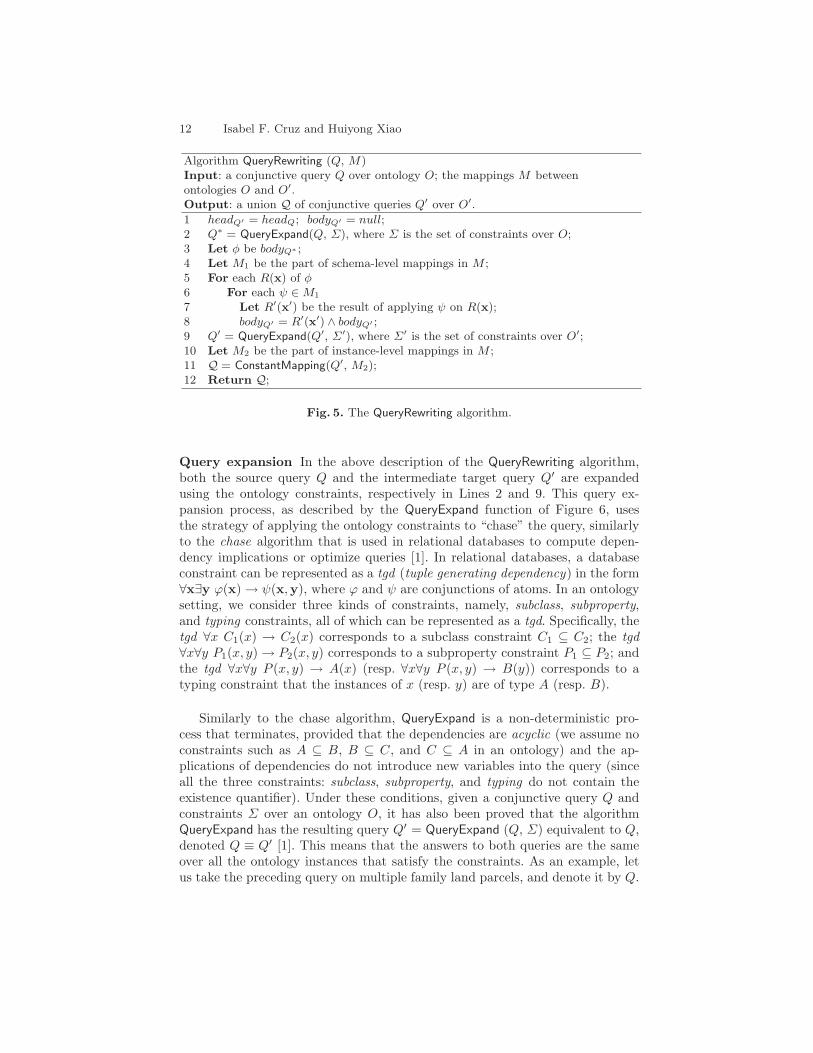
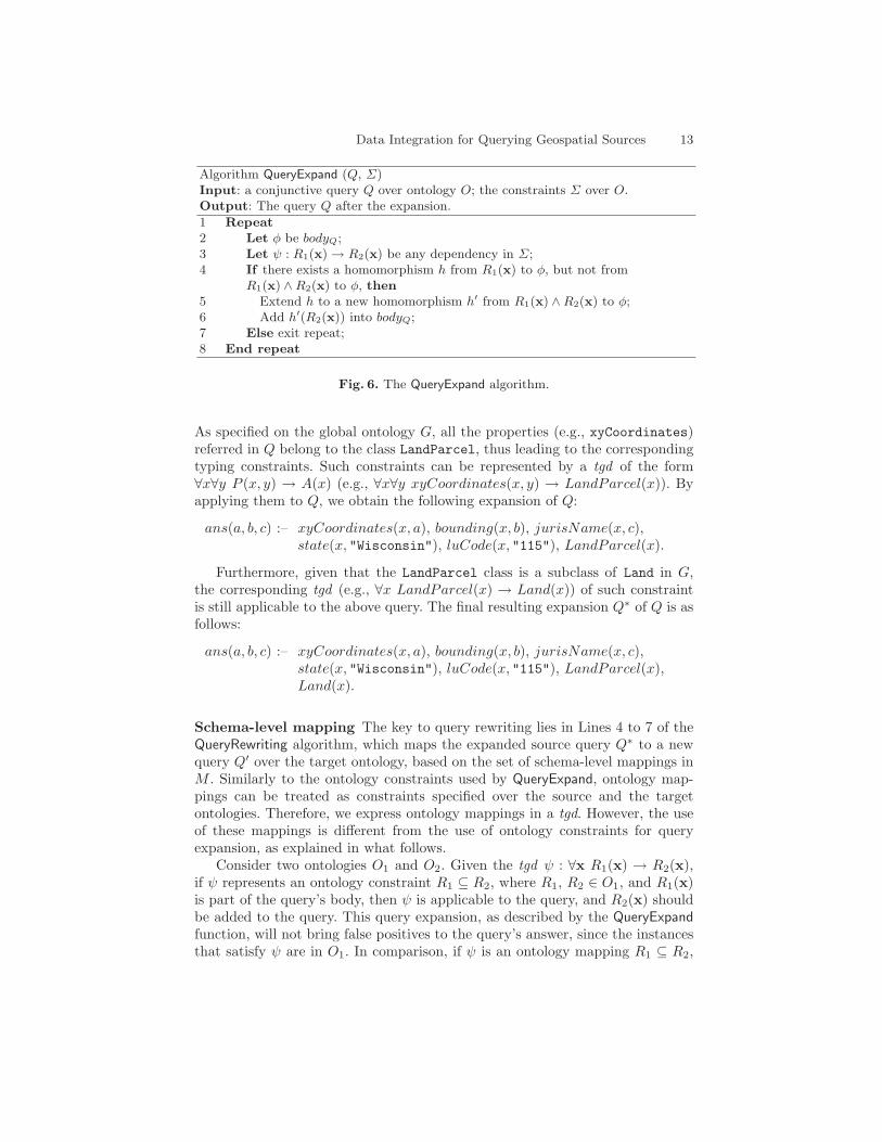
Algorithm QueryExpand (Q, Σ)Input: a conjunctive query Q over ontology O; the constraints Σ over O.Output: The query Q after the expansion.
1 Repeat2 Let φ be bodyQ;3 Let ψ : R1(x) → R2(x) be any dependency in Σ;4 If there exists a homomorphism h from R1(x) to φ, but not from
R1(x) ∧R2(x) to φ, then5 Extend h to a new homomorphism h′ from R1(x) ∧R2(x) to φ;6 Add h′(R2(x)) into bodyQ;7 Else exit repeat;8 End repeat
Fig. 6. The QueryExpand algorithm.
As specified on the global ontology G, all the properties (e.g., xyCoordinates)referred in Q belong to the class LandParcel, thus leading to the correspondingtyping constraints. Such constraints can be represented by a tgd of the form∀x∀y P (x, y) → A(x) (e.g., ∀x∀y xyCoordinates(x, y) → LandParcel(x)). Byapplying them to Q, we obtain the following expansion of Q:
ans(a, b, c) :– xyCoordinates(x, a), bounding(x, b), jurisName(x, c),state(x, "Wisconsin"), luCode(x, "115"), LandParcel(x).
Furthermore, given that the LandParcel class is a subclass of Land in G,the corresponding tgd (e.g., ∀x LandParcel(x) → Land(x)) of such constraintis still applicable to the above query. The final resulting expansion Q∗ of Q is asfollows:
ans(a, b, c) :– xyCoordinates(x, a), bounding(x, b), jurisName(x, c),state(x, "Wisconsin"), luCode(x, "115"), LandParcel(x),Land(x).
Schema-level mapping The key to query rewriting lies in Lines 4 to 7 of theQueryRewriting algorithm, which maps the expanded source query Q∗ to a newquery Q′ over the target ontology, based on the set of schema-level mappings inM . Similarly to the ontology constraints used by QueryExpand, ontology map-pings can be treated as constraints specified over the source and the targetontologies. Therefore, we express ontology mappings in a tgd. However, the useof these mappings is different from the use of ontology constraints for queryexpansion, as explained in what follows.
Consider two ontologies O1 and O2. Given the tgd ψ : ∀x R1(x) → R2(x),if ψ represents an ontology constraint R1 ⊆ R2, where R1, R2 ∈ O1, and R1(x)is part of the query’s body, then ψ is applicable to the query, and R2(x) shouldbe added to the query. This query expansion, as described by the QueryExpandfunction, will not bring false positives to the query’s answer, since the instancesthat satisfy ψ are in O1. In comparison, if ψ is an ontology mapping R1 ⊆ R2,
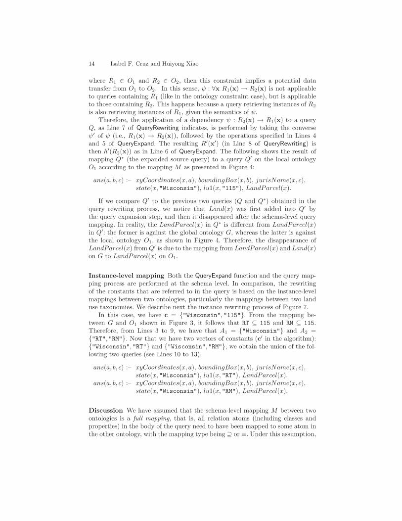
14 Isabel F. Cruz and Huiyong Xiao
where R1 ∈ O1 and R2 ∈ O2, then this constraint implies a potential datatransfer from O1 to O2. In this sense, ψ : ∀x R1(x) → R2(x) is not applicableto queries containing R1 (like in the ontology constraint case), but is applicableto those containing R2. This happens because a query retrieving instances of R2
is also retrieving instances of R1, given the semantics of ψ.Therefore, the application of a dependency ψ : R2(x) → R1(x) to a query
Q, as Line 7 of QueryRewriting indicates, is performed by taking the converseψ′ of ψ (i.e., R1(x) → R2(x)), followed by the operations specified in Lines 4and 5 of QueryExpand. The resulting R′(x′) (in Line 8 of QueryRewriting) isthen h′(R2(x)) as in Line 6 of QueryExpand. The following shows the result ofmapping Q∗ (the expanded source query) to a query Q′ on the local ontologyO1 according to the mapping M as presented in Figure 4:
ans(a, b, c) :– xyCoordinates(x, a), boundingBox(x, b), jurisName(x, c),state(x, "Wisconsin"), lu1(x, "115"), LandParcel(x).
If we compare Q′ to the previous two queries (Q and Q∗) obtained in thequery rewriting process, we notice that Land(x) was first added into Q′ bythe query expansion step, and then it disappeared after the schema-level querymapping. In reality, the LandParcel(x) in Q∗ is different from LandParcel(x)in Q′: the former is against the global ontology G, whereas the latter is againstthe local ontology O1, as shown in Figure 4. Therefore, the disappearance ofLandParcel(x) from Q′ is due to the mapping from LandParcel(x) and Land(x)on G to LandParcel(x) on O1.
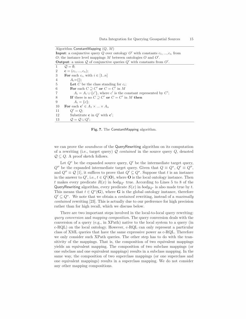
Instance-level mapping Both the QueryExpand function and the query map-ping process are performed at the schema level. In comparison, the rewritingof the constants that are referred to in the query is based on the instance-levelmappings between two ontologies, particularly the mappings between two landuse taxonomies. We describe next the instance rewriting process of Figure 7.
In this case, we have c = {"Wisconsin", "115"}. From the mapping be-tween G and O1 shown in Figure 3, it follows that RT ⊆ 115 and RM ⊆ 115.Therefore, from Lines 3 to 9, we have that A1 = {"Wisconsin"} and A2 ={"RT", "RM"}. Now that we have two vectors of constants (c′ in the algorithm):{"Wisconsin", "RT"} and {"Wisconsin", "RM"}, we obtain the union of the fol-lowing two queries (see Lines 10 to 13).
ans(a, b, c) :– xyCoordinates(x, a), boundingBox(x, b), jurisName(x, c),state(x, "Wisconsin"), lu1(x, "RT"), LandParcel(x).
ans(a, b, c) :– xyCoordinates(x, a), boundingBox(x, b), jurisName(x, c),state(x, "Wisconsin"), lu1(x, "RM"), LandParcel(x).
Discussion We have assumed that the schema-level mapping M between twoontologies is a full mapping, that is, all relation atoms (including classes andproperties) in the body of the query need to have been mapped to some atom inthe other ontology, with the mapping type being ⊇ or ≡. Under this assumption,
Data Integration for Querying Geospatial Sources 15
Algorithm ConstantMapping (Q, M)Input: a conjunctive query Q over ontology O′ with constants c1, ..., cn fromO; the instance level mappings M between ontologies O and O′.Output: a union Q of conjunctive queries Q′ with constants from O′.1 Q = ∅;2 c = (c1, ..., cn);3 For each ci, with i ∈ [1..n]4 Ai={};5 Let C be the class standing for ci;6 For each C ⊇ C′ or C = C′ in M7 Ai = Ai ∪ {c′}, where c′ is the constant represented by C′;8 If there is no C ⊇ C′ or C = C′ in M then9 Ai = {c};10 For each c′ ∈ A1 × ...×An
11 Q′ = Q;12 Substitute c in Q′ with c′;13 Q = Q∪Q′;
Fig. 7. The ConstantMapping algorithm.
we can prove the soundness of the QueryRewriting algorithm on its computationof a rewriting (i.e., target query) Q contained in the source query Q, denotedQ ⊆ Q. A proof sketch follows.
Let Q∗ be the expanded source query, Q′ be the intermediate target query,Q′′ be the expanded intermediate target query. Given that Q ≡ Q∗, Q′ ≡ Q′′,and Q′′ ≡ Q [1], it suffices to prove that Q′ ⊆ Q∗. Suppose that t is an instancein the answer to Q′, i.e., t ∈ Q′(O), where O is the local ontology instance. Thent makes every predicate R(x) in bodyQ′ true. According to Lines 5 to 8 of theQueryRewriting algorithm, every predicate S(x) in bodyQ∗ is also made true by t.This means that t ∈ Q∗(G), where G is the global ontology instance, thereforeQ′ ⊆ Q∗. We note that we obtain a contained rewriting, instead of a maximallycontained rewriting [23]. This is actually due to our preference for high precisionrather than for high recall, which we discuss below.
There are two important steps involved in the local-to-local query rewriting:query conversion and mapping composition. The query conversion deals with theconversion of a query (e.g., in XPath) native to the local system to a query (inc-RQL) on the local ontology. However, c-RQL can only represent a particularclass of XML queries that have the same expressive power as c-RQL. Thereforewe only consider such XPath queries. The other step has to do with the tran-sitivity of the mappings. That is, the composition of two equivalent mappingsyields an equivalent mapping. The composition of two subclass mappings (orone subclass and one equivalent mappings) results in a subclass mapping. In thesame way, the composition of two superclass mappings (or one superclass andone equivalent mappings) results in a superclass mapping. We do not considerany other mapping compositions.
16 Isabel F. Cruz and Huiyong Xiao
The last issue we discuss relates to the trade-off between the precision andrecall of the query processing. Currently, the the query rewriting algorithm onlyuses mappings that guarantee the correctness of the query. For instance, given aquery Q : {x|A(x)}, our query rewriting algorithm only rewrites Q to {x|B(x)}in two cases: A ⊇ B or A ≡ B. This ensures that we will not return to the userinstances that do not belong to A. But we may miss some instances of B thatare also instances of A and should be included in the answer to Q, thus loweringrecall. An alternative is to allow the approximate semantic relationship and toassign a score between [0..1] to every mapping based on the similarity of themapped classes or properties. Thus, query rewriting can calculate an estimatedprecision of the target query. In practice, different scenarios impose differentrequirements on the mappings. For example, an eCommerce application involv-ing purchase orders requires a very precise and complete translation of a query,whereas a search engine usually does not require an exact transformation [8].
6 User Interfaces
In this section, we briefly describe the two user interfaces that assist respectivelyin ontology alignment (and in particular instance-level mapping) and in queryprocessing.
6.1 Visual Ontology Alignment
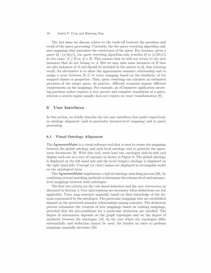
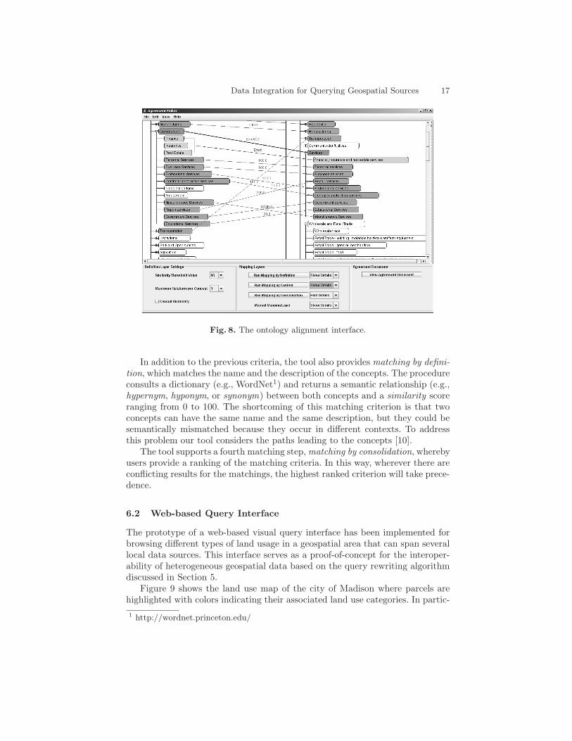
The AgreementMaker is a visual software tool that is used to create the mappingsbetween the global ontology and each local ontology and to generate the agree-ment documents [9]. With this tool, users load two ontologies side-by-side anddisplay each one as a tree of concepts as shown in Figure 8. The global ontologyis displayed on the left hand side and the local (target) ontology is displayed onthe right hand side. Concept (or class) names are displayed in rectangular nodeson the ontological trees.
The AgreementMaker implements a hybrid ontology matching process [28], bycombining several matching methods to determine the schema-level and instance-level mappings between both ontologies.
The first two criteria are the rule-based deduction and the user interaction, asdiscussed in Section 4. User interventions are necessary when deductions are notapplicable. Users map concepts manually based on their knowledge of the do-main represented by the ontologies. The particular mappings that are establisheddepend on the perceived semantic relationships among concepts. The deductionprocess automates the creation of new mappings based on existing mappings,provided that the pre-conditions for a particular deduction are satisfied. Thedegree of automation depends on the graph topologies and on the degree ofsimilarity between the ontologies [10]. In the case where the topologies differsubstantially and deduction cannot be used, the burden on users to performmappings manually increases [25].
Data Integration for Querying Geospatial Sources 17
Fig. 8. The ontology alignment interface.
In addition to the previous criteria, the tool also provides matching by defini-tion, which matches the name and the description of the concepts. The procedureconsults a dictionary (e.g., WordNet1) and returns a semantic relationship (e.g.,hypernym, hyponym, or synonym) between both concepts and a similarity scoreranging from 0 to 100. The shortcoming of this matching criterion is that twoconcepts can have the same name and the same description, but they could besemantically mismatched because they occur in different contexts. To addressthis problem our tool considers the paths leading to the concepts [10].
The tool supports a fourth matching step, matching by consolidation, wherebyusers provide a ranking of the matching criteria. In this way, wherever there areconflicting results for the matchings, the highest ranked criterion will take prece-dence.
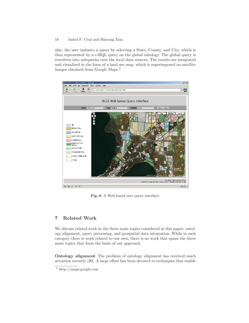
6.2 Web-based Query Interface
The prototype of a web-based visual query interface has been implemented forbrowsing different types of land usage in a geospatial area that can span severallocal data sources. This interface serves as a proof-of-concept for the interoper-ability of heterogeneous geospatial data based on the query rewriting algorithmdiscussed in Section 5.
Figure 9 shows the land use map of the city of Madison where parcels arehighlighted with colors indicating their associated land use categories. In partic-1 http://wordnet.princeton.edu/
18 Isabel F. Cruz and Huiyong Xiao
ular, the user initiates a query by selecting a State, County, and City, which isthen represented by a c-RQL query on the global ontology. The global query isrewritten into subqueries over the local data sources. The results are integratedand visualized in the form of a land use map, which is superimposed on satelliteimages obtained from Google Maps.2
Fig. 9. A Web-based user query interface.
7 Related Work
We discuss related work in the three main topics considered in this paper: ontol-ogy alignment, query processing, and geospatial data integration. While in eachcategory there is work related to our own, there is no work that spans the threemain topics that form the basis of our approach.
Ontology alignment The problem of ontology alignment has received muchattention recently [30]. A large effort has been devoted to techniques that enable
2 http://maps.google.com
Data Integration for Querying Geospatial Sources 19
the automatic (or semi-automatic) alignment of concepts across ontologies [15].Existing alignment approaches make use of one or more ontology alignment (ormatching) techniques belonging to the following three categories:
Element-level At the element level, matching can use various similarity mea-sures based, for example, on names of elements or their textual descriptions.A normalized numerical value is calculated for each of the matching candi-dates, and the best one is selected [4, 6, 26].
Structure-level The structure-level information that can be used by the match-ing process include the graph or taxonomy underlying the schema or ontol-ogy. Graphs are used as contextual information to map pairs of elements andthe taxonomy can provide the matching process with more semantics [24, 25].An example of semantic-level matching determines the similarity of two con-cepts based on the similarities of their ancestors [29]. In our approach, weconsider the semantic similarity of the concepts’ children, instead.
Instance-level Instance-level matching uses the actual contents (or instances)of the schema or ontology elements [12, 21].
Although we have two types of ontologies to align, namely the schema-like on-tologies and the taxonomy-like ontologies, in this paper we have mainly concen-trated on the alignment of the latter type. Taxonomy-like ontologies use only thesubconcept (or subclass) relationships between two entities, therefore they lendthemselves well to the use of structure-level methods. However, element-leveland instance-level approaches can be used in conjunction with our structure-level methods. In fact, our prototype makes use of element-level alignment asdescribed in Section 6.
Related systems to ours include Clio [20], COMA++ [3], and Falcon-AO [22].The first two place a strong emphasis on the user interface, like we do, whilethe last two share with our approach their support for structure-level automaticmatching methods.
Query processing When mappings are defined as (relational) views, queryprocessing is often referred in the literature as view-based query answering orrewriting [19]. However, few view-based query processing algorithms address theissue of query rewriting over ontologies involving the specific kinds of issuesinvolved, which we must take into account [31].
Schema and ontology-based query processing techniques have been proposedboth for centralized [2, 27, 34] and for peer-to-peer architectures [5, 13, 16].While most of these approaches focus on XML or relational query languages toperform the query rewriting, we use RQL because of our choice of metadata anddata representation.
Our ontology-based query rewriting algorithm is similar to the computeWTAalgorithm proposed by Calvanese et al. for query reformulation [5] as both as-sume consistent ontology mappings. However, we allow for the transformation ofthe values that are contained in the query based on the instance-level ontologymappings. In this way, we can address semantic heterogeneity, which occurs inthe land use codes.
20 Isabel F. Cruz and Huiyong Xiao
Another related approach considers constraint-based query processing in theClio system [34]. It focuses on schema mapping and data transformation betweennested (XML) schemas and relational databases by taking advantage of theschema semantics to generate consistent translations from source to target andby considering the constraints and structure of the target schema.
Geospatial data integration Information integration methodology from thedatabase community has been applied to spatial information systems. For ex-ample, the MIX framework offers a meditation approach for integrating het-erogeneous sources containing spatial data types (e.g., vector graphics, maps)and associated data (e.g., text, tables, figures, images) [18], which supports awide range of spatial applications. The system architecture comprises three lay-ers: a foundation layer consisting of databases and wrappers, a mediation layersupporting query and result exchange among the wrapped sources, and an appli-cation/user interface layer. In the foundation layer, the data model is exportedfrom the sources in the form of an XML DTD. In the case of spatial information,for example, the wrapper constructs the DTD by using the associated cataloginformation. The wrappers support scripts that execute complex queries as acombination of several primitive queries. As compared to our approach, seman-tic relationships are supported, for example in the form of spatial predicatessuch as within(region1,region2), but there is not an overall “semantic graph”that would support, for example, the alignment of spatial attributes.
VirGIS is a more recent approach for mediation of geographical informationsystems [14]. It differs from MIX in that it adopts newer standards such asGML (Geography Markup Language) for data modeling and WFS (Web Fea-ture Servers) to perform communications (e.g., queries) with clients. It supportsmappings between attributes or classes but no semantic overall framework ispresented.
8 Conclusions
In this paper, we focused on data integration and interoperability across dis-tributed geospatial data sources. To illustrate the impact of our approach weshowed practical examples that are derived from land use applications.
We propose an ontology-based approach to achieve the integration and inter-operability of the distributed geospatial data sources by solving both schematicand semantic heterogeneities. Two different kinds of mappings are establishedbetween the global ontology (which describes the domain) and each local ontol-ogy (which describes each data source): schema mappings between the schemaof both ontologies and instance mappings between the (land use) taxonomies ofboth ontologies.
We have discussed two modes of query processing in our system, global-to-local and local-to-local (or peer-to-peer). Query rewriting in both modes uses thepreviously established mappings. We propose a c-RQL (conjunctive RQL) query
Data Integration for Querying Geospatial Sources 21
rewriting algorithm, such that the resulting target query is contained in thesource query, thus providing sound answers to the source query.
Future work will focus on:
– Ontology alignment, and in particular the deduction-based method. Cur-rently, we make some assumptions on the topology of the ontologies. Withoutsuch assumptions, we may need to consider the combination of our bottom-up deduction process with top-down reasoning on mappings (e.g., [29]).
– Query rewriting, so as to take into account “approximate” mappings. In thiscase, precision and recall of query answering will depend on the similarityof the underlying mappings, thus making the ability to determine mappingsimilarities a critical task.
9 Acknowledgements
We would like to thank Nancy Wiegand and Steve Ventura, from the Land Infor-mation & Computer Graphics Facility at the University of Wisconsin-Madison,and the members of WLIS for discussions on land use and other scenarios relatedto geospatial data integration. We would also like to thank Sujan Bathala, NalinMakar, Afsheen Rajendran, and William Sunna for their help with the designand implementation of the user interfaces.
Bibliography
[1] S. Abiteboul, R. Hull, and V. Vianu. Foundations of Databases. Addison-Wesley, 1995.
[2] B. Amann, C. Beeri, I. Fundulaki, and M. Scholl. Querying XML SourcesUsing an Ontology-Based Mediator. In Confederated International Confer-ences DOA, CoopIS and ODBASE, volume 2519 of Lecture Notes in Com-puter Science, pages 429–448. Springer, 2002.
[3] D. Aumueller, H. H. Do, S. Massmann, and E. Rahm. Schema and OntologyMatching with COMA++. In ACM SIGMOD International Conference onManagement of Data, pages 906–908, 2005.
[4] S. Bergamaschi, S. Castano, and M. Vincini. Semantic Integration ofSemistructured and Structured Data Sources. SIGMOD Record, 28(1):54–59, 1999.
[5] D. Calvanese, G. D. Giacomo, D. Lembo, M. Lenzerini, and R. Rosati.What to Ask to a Peer: Ontology-based Query Reformulation. In Interna-tional Conference on Principles of Knowledge Representation and Reason-ing (KR), pages 469–478, 2004.
[6] S. Castano, V. D. Antonellis, and S. D. C. di Vimercati. Global Viewing ofHeterogeneous Data Sources. IEEE Transactions on Knowledge and DataEngineering, 13(2):277–297, 2001.
[7] V. Christophides, G. Karvounarakis, I. Koffina, G. Kokkinidis, A. Magka-naraki, D. Plexousakis, G. Serfiotis, and V. Tannen. The ICS-FORTHSWIM: A Powerful Semantic Web Integration Middleware. In InternationalWorkshop on Semantic Web and Databases (SWDB), pages 381–393, 2003.
[8] V. Cross. Uncertainty in the Automation of Ontology Matching. In In-ternational Symposium on Uncertainty Modeling and Analysis (ISUMA),pages 135–140, 2003.
[9] I. F. Cruz, W. Sunna, and A. Chaudhry. Semi-Automatic Ontology Align-ment for Geospatial Data Integration. In International Conference on Geo-graphic Information Science (GIScience), volume 3234 of Lecture Notes inComputer Science, pages 51–66. Springer, 2004.
[10] I. F. Cruz, W. G. Sunna, and K. Ayloo. Concept Level Matching of Geospa-tial Ontologies. In GIS Planet International Conference and Exhibition onGeographic Information, 2005.
[11] I. F. Cruz, H. Xiao, and F. Hsu. An Ontology-based Framework for Se-mantic Interoperability between XML Sources. In International DatabaseApplications and Engineering Symposium (IDEAS), pages 217–226, July2004.
[12] A. Doan, J. Madhavan, P. Domingos, and A. Y. Halevy. Learning to Mapbetween Ontologies on the Semantic Web. In International World WideWeb Conference (WWW), pages 662–673, 2002.
[13] M. Ehrig, C. Tempich, J. Broekstra, F. van Harmelen, M. Sabou, R. Siebes,S. Staab, and H. Stuckenschmidt. SWAP - Ontology-based Knowledge Man-
Data Integration for Querying Geospatial Sources 23
agement with Peer-to-Peer Technology. In German Workshop on Ontology-based Knowledge Management (WOW), 2003.
[14] M. Essid, F.-M. Colonna, O. Boucelma, and A. Betari. Querying Medi-ated Geographic Data Sources. In International Conference on ExtendingDatabase Technology (EDBT), volume 3896 of Lecture Notes in ComputerScience, pages 1176–1181. Springer, 2006.
[15] J. Euzenat, A. Isaac, C. Meilicke, P. Shvaiko, H. Stuckenschmidt, O. Svab,V. Svatek, W. R. van Hage, and M. Yatskevich. First Results of the Ontol-ogy Evaluation Initiative 2007. In Second ISWC International Workshopon Ontology Matching. CEUR-WS, 2007.
[16] E. Franconi, G. M. Kuper, A. Lopatenko, and I. Zaihrayeu. A DistributedAlgorithm for Robust Data Sharing and Updates in P2P Database Net-works. In Current Trends in Database Technology - EDBT 2004 Workshops,Lecture Notes in Computer Science, pages 446–455. Springer, 2004.
[17] T. R. Gruber. A Translation Approach to Portable Ontology Specifications.Knowledge Acquisition, 5(2):199–220, 1993.
[18] A. Gupta, R. Marciano, I. Zaslavsky, and C. K. Baru. Integrating GISand Imagery Through XML-Based Information Mediation. In InternationalWorkshop on Integrated Spatial Databases (ISD), Selected Papers, volume1737 of Lecture Notes in Computer Science, pages 211–234. Springer, 1999.
[19] A. Y. Halevy. Answering Queries Using Views: A Survey. VLDB Journal,10(4):270–294, 2001.
[20] M. A. Hernandez, R. J. Miller, and L. M. Haas. Clio: A Semi-AutomaticTool For Schema Mapping (demo). In ACM SIGMOD International Con-ference on Management of Data, page 607, 2001.
[21] R. Ichise, H. Takeda, and S. Honiden. Rule Induction for Concept HierarchyAlignment. In IJCAI Workshop on Ontologies and Information Sharing,2001.
[22] N. Jian, W. Hu, G. Cheng, and Y. Qu. Falcon-AO: Aligning Ontologieswith Falcon. In K-CAP 2005 Workshop on Integrating Ontologies. CEURWorkshop Proceedings 156, 2005.
[23] M. Lenzerini. Data Integration: A Theoretical Perspective. In ACMSIGMOD-SIGACT-SIGART Symposium on Principles of Database Systems(PODS), pages 233–246, 2002.
[24] S. Melnik, H. Garcia-Molina, and E. Rahm. Similarity Flooding: A VersatileGraph Matching Algorithm and Its Application to Schema Matching. InIEEE International Conference on Data Engineering (ICDE), pages 117–128, 2002.
[25] N. F. Noy and M. A. Musen. Anchor-PROMPT: Using Non-local Contextfor Semantic Matching. In IJCAI Workshop on Ontologies and InformationSharing, 2001.
[26] L. Palopoli, D. Sacca, and D. Ursino. An Automatic Techniques for Detect-ing Type Conflicts in Database Schemes. In International Conference onInformation and Knowledge Management (CIKM), pages 306–313, 1998.
[27] M. Peim, E. Franconi, N. W. Paton, and C. A. Goble. Query Processingwith Description Logic Ontologies Over Object-Wrapped Databases. In In-
24 Isabel F. Cruz and Huiyong Xiao
ternational Conference on Scientific and Statistical Database Management(SSDBM), pages 27–36, 2002.
[28] E. Rahm and P. A. Bernstein. A Survey of Approaches to AutomaticSchema Matching. VLDB Journal, 10(4):334–350, 2001.
[29] M. A. Rodrıguez and M. J. Egenhofer. Determining Semantic Similarityamong Entity Classes from Different Ontologies. IEEE Transactions onKnowledge and Data Engineering, 15(2):442–456, 2003.
[30] P. Shvaiko and J. Euzenat. A Survey of Schema-Based Matching Ap-proaches. In Journal on Data Semantics IV, volume 3730 of Lecture Notesin Computer Science, pages 146–171. Springer, 2005.
[31] H. Stuckenschmidt. Query Processing on the Semantic Web. KunstlicheIntelligenz (KI), 17(3):22–26, 2003.
[32] H. Wache, T. Vogele, U. Visser, H. Stuckenschmidt, G. Schuster, H. Neu-mann, and S. Hubner. Ontology-Based Integration of Information - A Sur-vey of Existing Approaches. In IJCAI Workshop on Ontologies and Infor-mation Sharing, 2001.
[33] N. Wiegand, D. Patterson, N. Zhou, S. Ventura, and I. F. Cruz. Query-ing Heterogeneous Land Use Data: Problems and Potential. In NationalConference for Digital Government Research (dg.o), pages 115–121, 2002.
[34] C. Yu and L. Popa. Constraint-Based XML Query Rewriting For DataIntegration. In ACM SIGMOD International Conference on Managementof Data, pages 371–382, 2004.