Embed Size (px)
Citation preview
Data forHelioseismology Testing
Dali GeorgobianiMichigan State University
Presenting the results of
Bob Stein (MSU) & Åke Nordlund (NBI, Denmark)with
David Benson (Kettering University)
Stanford, July 29, 2008
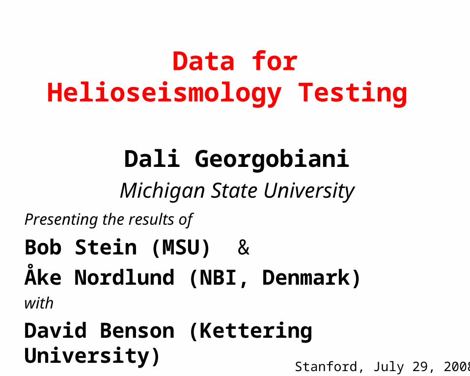
Numerical Method
Staggered mesh
Non-linear, fully compressible, 3D, explicit
Spatial differencing:
6th order centered finite difference
Time advancement:
3rd order Runge-Kutta
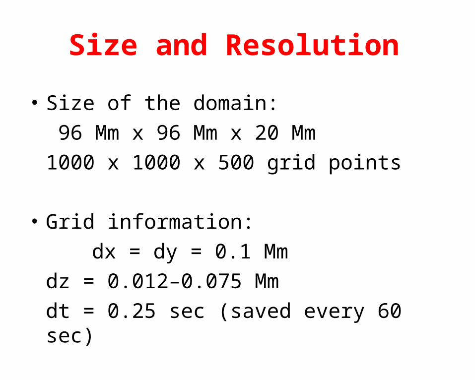
Size and Resolution
• Size of the domain:
96 Mm x 96 Mm x 20 Mm
1000 x 1000 x 500 grid points
• Grid information:
dx = dy = 0.1 Mm
dz = 0.012–0.075 Mm
dt = 0.25 sec (saved every 60 sec)
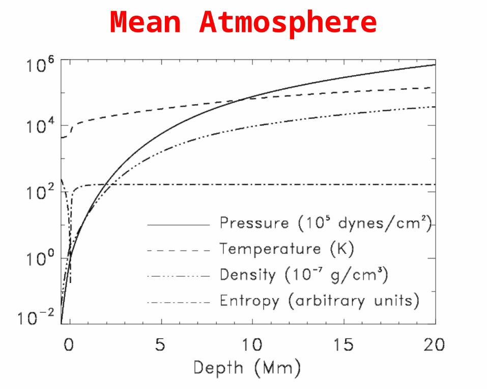
Mean Atmosphere
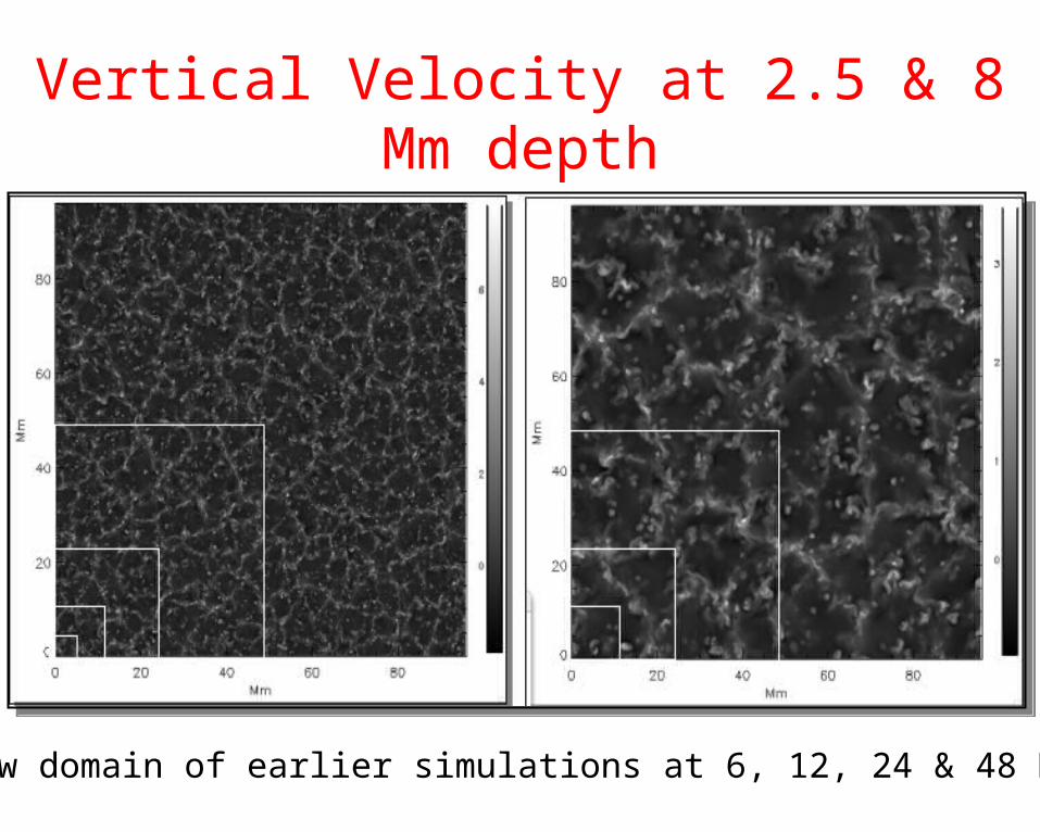
Vertical Velocity at 2.5 & 8 Mm depth
Boxes show domain of earlier simulations at 6, 12, 24 & 48 Mm widths.
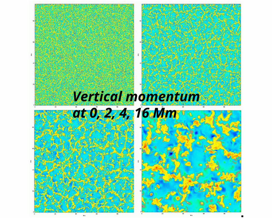
Vertical momentum at 0, 2, 4, 16 Mm
Vertical momentum vs depth
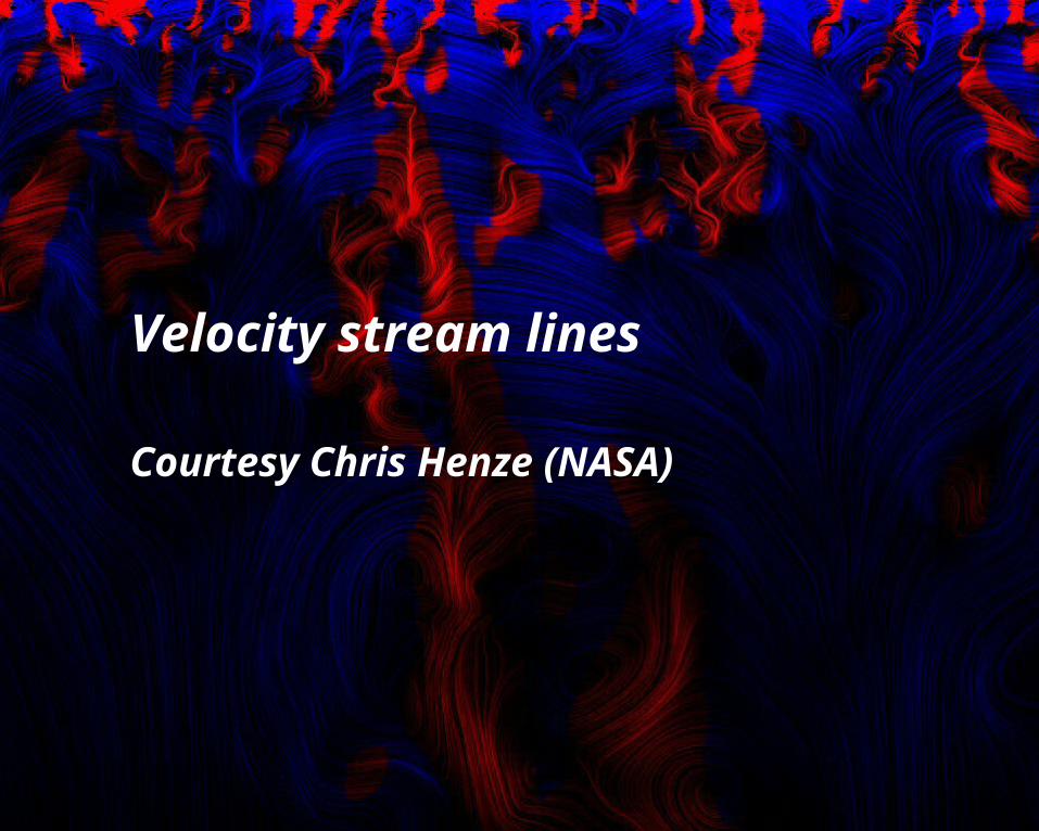
Velocity stream lines
Courtesy Chris Henze (NASA)
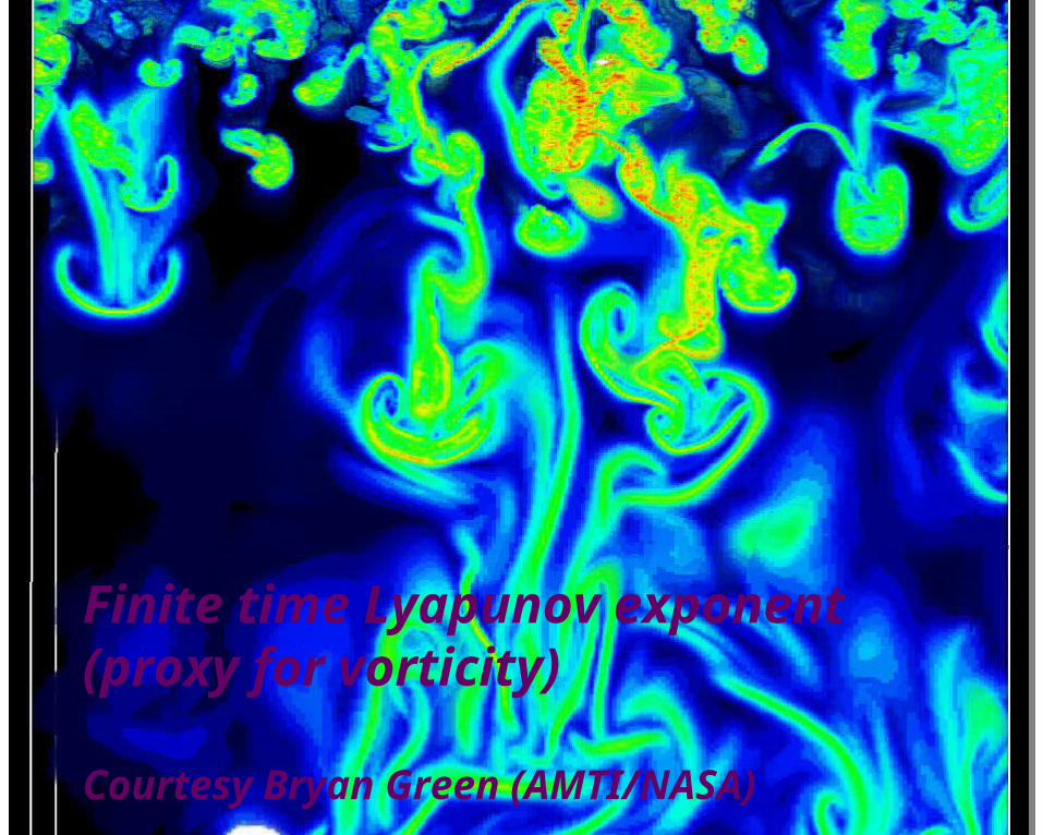
Finite time Lyapunov exponent(proxy for vorticity)
Courtesy Bryan Green (AMTI/NASA)
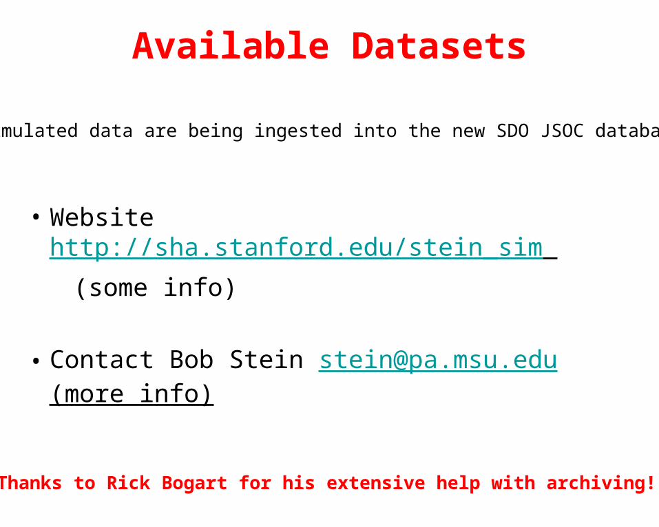
Available Datasets
• Website http://sha.stanford.edu/stein_sim
(some info)
• Contact Bob Stein [email protected] (more info)
Simulated data are being ingested into the new SDO JSOC database
Thanks to Rick Bogart for his extensive help with archiving!
Archived Data Description
• 9 variables: horizontal velocities Vx, Vz, vertical velocity Vy, temperature, density, pressure, internal energy, electron density, and
• Each snapshot of a variable is stored in a separate file; 9 variables at each time step are combined to be retrieved together
• Data are in FITS format
• Duration 511 minutes (360 minutes recorded, WIP)
• A snapshot of a variable occupies approximately 2 GB of disk space
• First and third directions are horizontal, second direction is vertical
• Vertical grid is provided separately
(The data will be available for retrieval soon – check with Rick)
Another Data Set
• 4 hour averages, with 2 hour overlap
• 6 variables: horizontal velocities Vx, Vz, vertical velocity Vy, temperature, density, and sound speed
• Simultaneous surface velocities
• Stored in the IDL SAVE format at MSU
• Work in progress… initial 6 variables calculated and stored, now adding internal energy E
Units of Variables
• Length is in 108 cm = 1 Mm
• Time is in 102 s
• Velocities Vx, Vz, and Vy are in 10 km/s
• Temperature is in K
• Density is in 10-7 g/cm3
• Pressure is in 105 dynes/cm2
• Internal energy is in 105 ergs/cm3
• Electron density is log cm-3
Data Analysis
• Power spectrum
• Tests of time-distance methods
Compare the results for the simulations and
the SOHO/MDI high-res observations
(211.5 Mm by 211.5 Mm patch, 512 min)
The following work was performed with
Junwei Zhao and Alexander Kosovichev
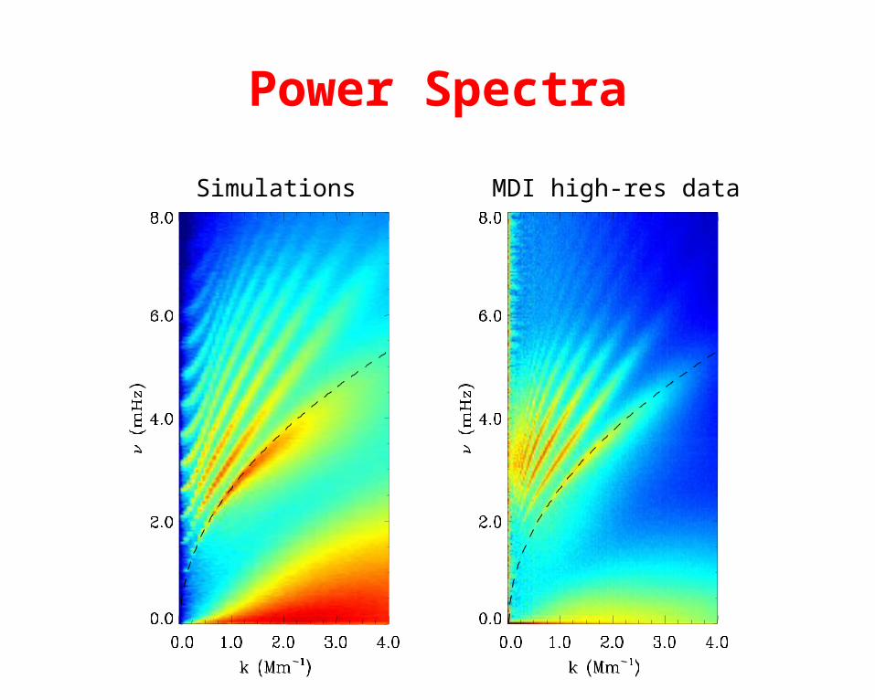
Power Spectra
Simulations MDI high-res data
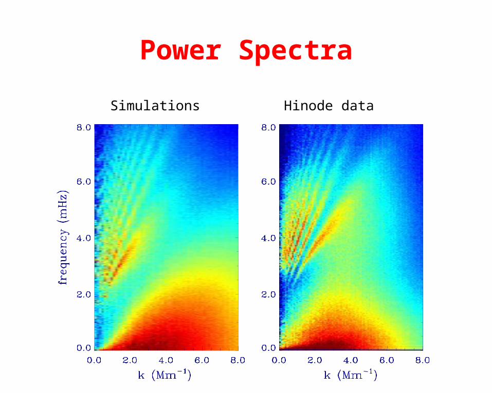
Power Spectra
Simulations Hinode data
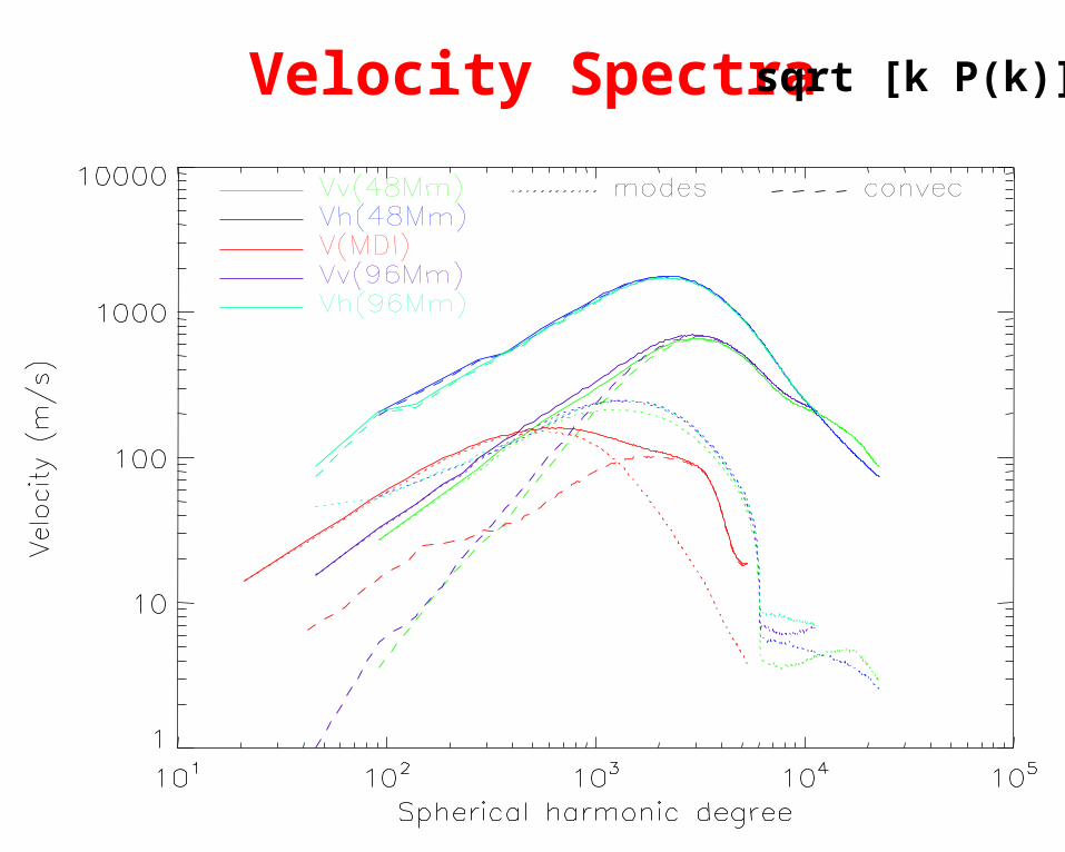
Velocity Spectra sqrt [k P(k)]
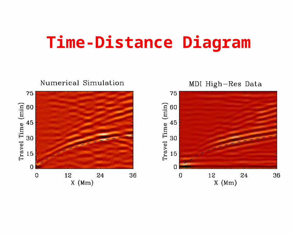
Time-Distance Diagram
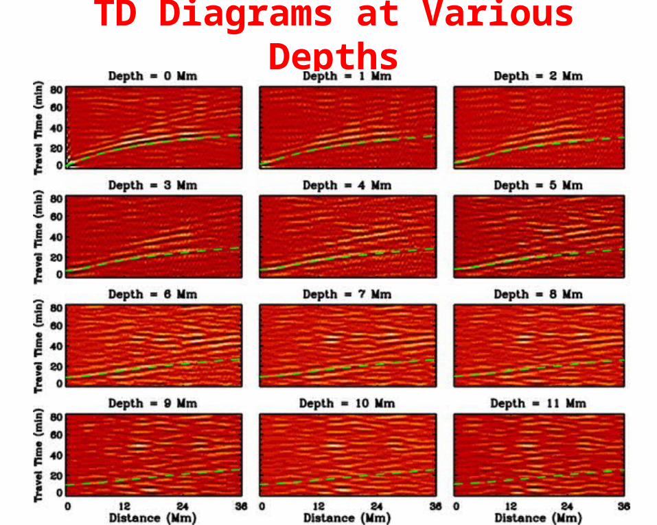
TD Diagrams at Various Depths
Exploring Simulated Surface Structures
• Spatial filtering
• Spectral analysis
• f-mode time-distance analysis
• Local correlation tracking
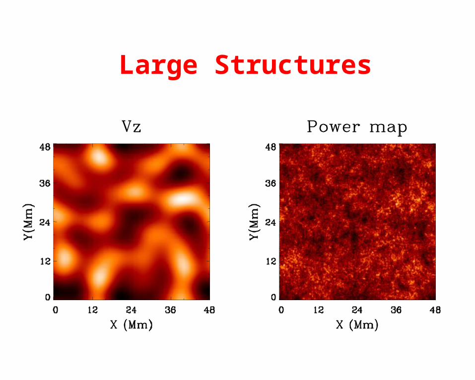
Large Structures
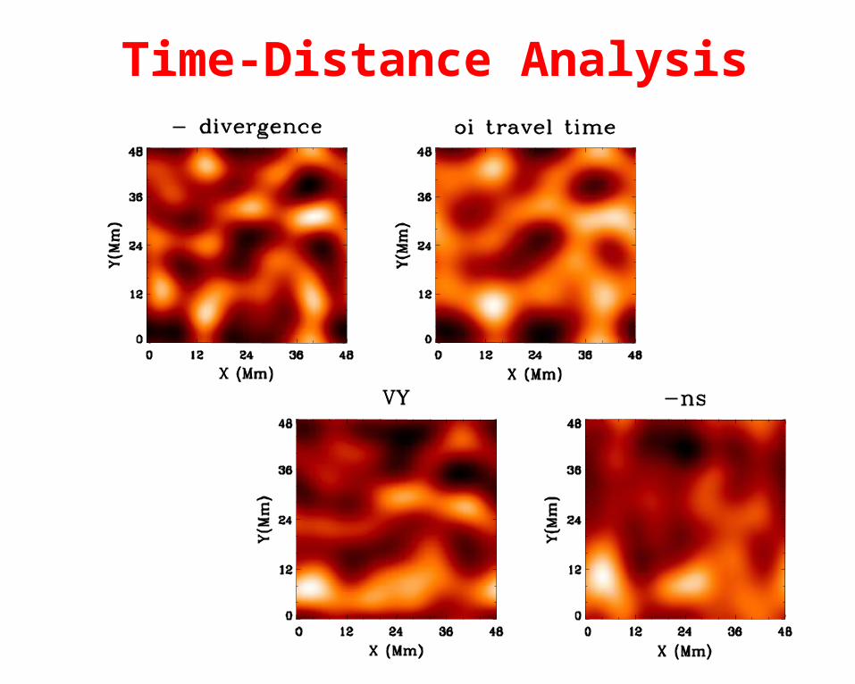
Time-Distance Analysis
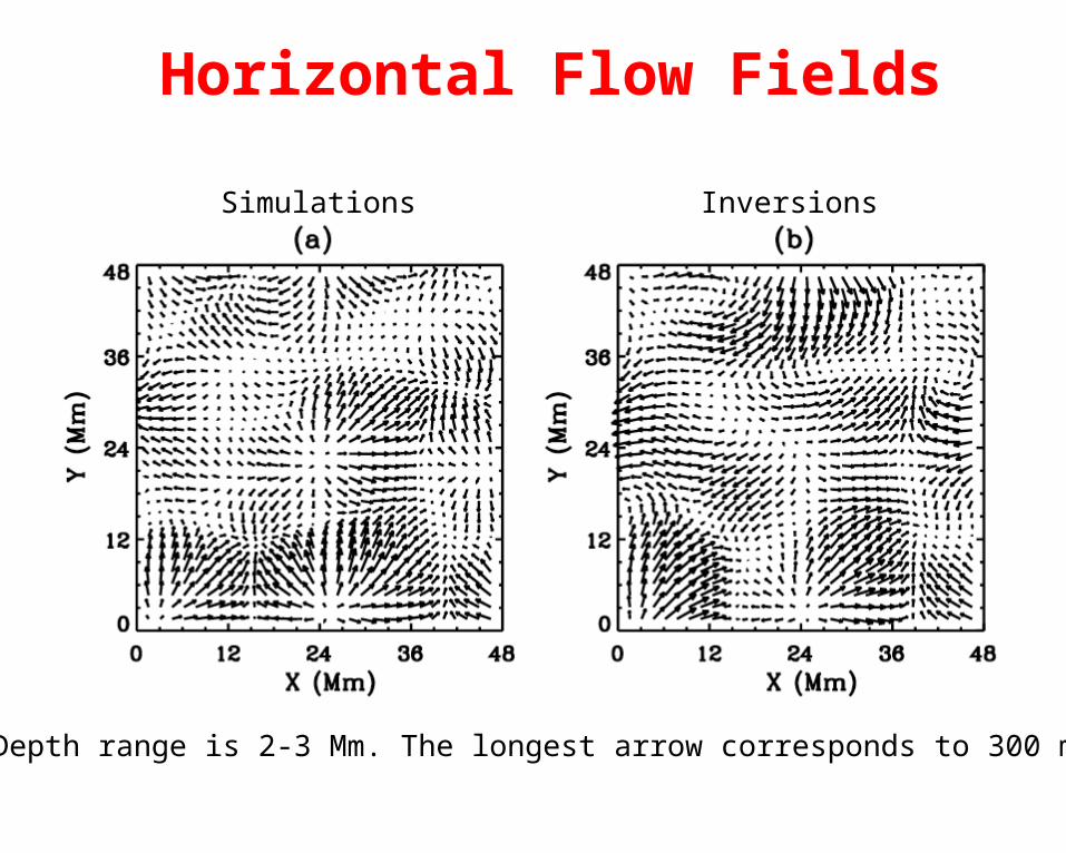
Horizontal Flow Fields
Simulations Inversions
Depth range is 2-3 Mm. The longest arrow corresponds to 300 m/s
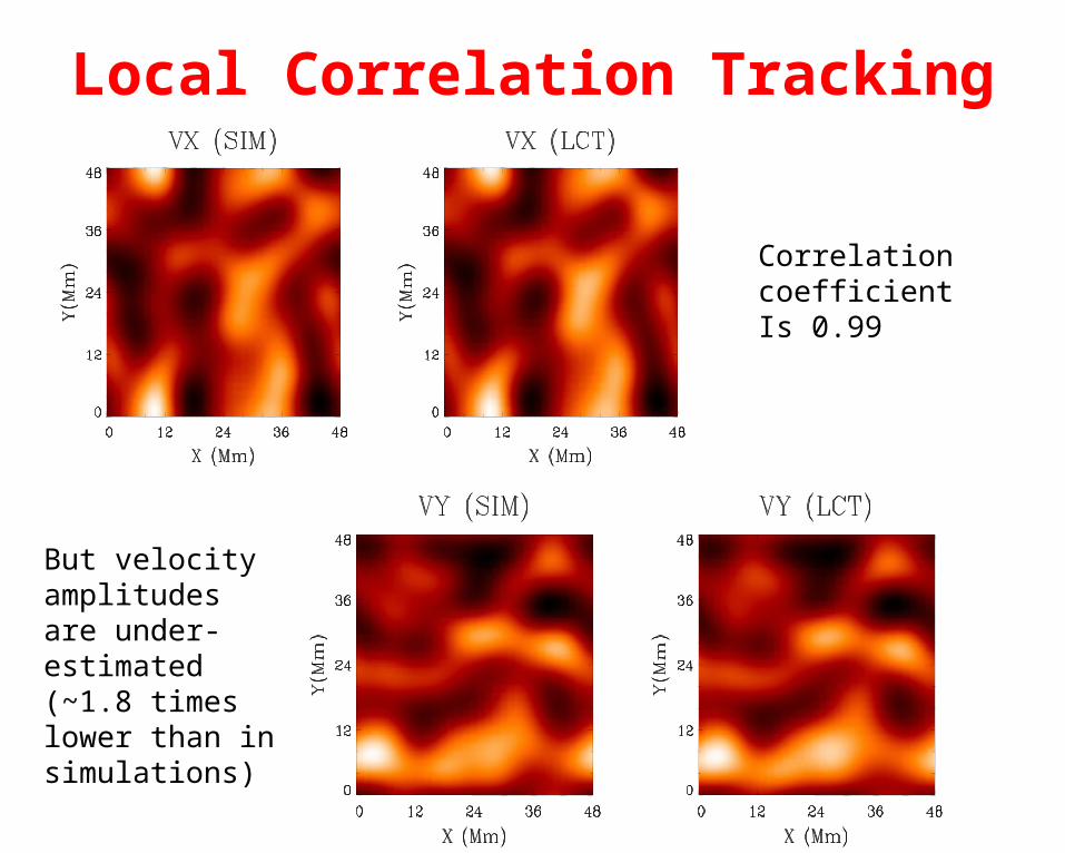
Local Correlation Tracking
CorrelationcoefficientIs 0.99
But velocityamplitudes are under-estimated(~1.8 timeslower than in simulations)
These simulations provide an excellentopportunity to validate various techniques, widely used in solar physics and helio-seismology for directly obtaining otherwise inaccessible properties (subsurfaceflows, structures etc.)
On the other hand, these analysis techniques also help to examinehow realistic the simulations are
Conclusions