Embed Size (px)
Citation preview
1
Data Driven Modellingfor Complex Systems
Dr Hua-Liang (Leon) Wei
Senior Lecturer in System Identification and Data Analytics
Head of Dynamic Modelling, Data Mining & Decision Making (3DM) Lab
Complex Systems & Signal Processing Research Group
Department of Automatic Control & System Engineering
University of Sheffield
Sheffield, UKJuly 26-28, 2017 HLW, Data Based Modelling, Slide 1 of 45
Data Driven Modelling
Similar Terminologies:
• Black-box Modelling
• Data-based Modelling
• Learning from Data
• System Identification
…, etc.
July 26-28, 2017 HLW, Data Based Modelling, Slide 2 of 45

2
Outline of the Talk
2) Three classes of models
─ White, grey and black-box models
3) Data-driven modelling
─ Letting data speak and learning from data
4) Examples
─ Using data-driven modelling techniques
1) A quick selective review of system models─ Model types and generalised linear models
July 26-28, 2017 HLW, Data Based Modelling, Slide 3 of 45
PART 1
A Quick Selective Review
of
System Models
July 26-28, 2017 HLW, Data Based Modelling, Slide 4 of 45

3
Linear vs NonlinearLinear Systems Nonlinear Systems
Linear systems are simple systems whose structure and behavior are regular and easy to understand.
Nonlinear systems are complex systems whose structure and behavior are normally difficult to analyse.
July 26-28, 2017
Linear vs Nonlinear Models
Linear Models
• Continuous-time model
• Continuous-time state space
• Continuous-time transferfunction
Nonlinear Models♦ Continuous-time NL model
♦ Continuous-time NL state space
♦ Continuous-time transfer functionfor a nonlinear system? (No, not really!)
• Discrete-time model
• Discrete-time transfer function (e.g. Z-transfer function)
• Discrete-time state space
♦ Discrete-time NL model
♦ Discrete-time NL state space
♦ Discrete-time transfer function for nonlinear systems? (No, not really!)
July 26-28, 2017 Dr HL Wei, Data Based Modelling, Slide 6 of 45
4
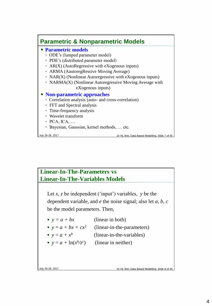
Parametric & Nonparametric Models
• Parametric models◦ ODE’s (lumped parameter model)
◦ PDE’s (distributed parameter model)
◦ AR(X) (AutoRegressive with eXogenous inputs)
◦ ARMA (AautoregRessive Moving Average)
◦ NAR(X) (Nonlinear Autoregressive with eXogenous inputs)
◦ NARMA(X) (Nonlinear Autoregressive Moving Average with
eXogenous inputs)
• Non-parametric approaches◦ Correlation analysis (auto- and cross-correlation)
◦ FFT and Spectral analysis
◦ Time-frequency analysis
◦ Wavelet transform
◦ PCA, ICA, …
◦ Bayesian, Gaussian, kernel methods, … etc.
July 26-28, 2017 Dr HL Wei, Data Based Modelling, Slide 7 of 45
Linear-In-The-Parameters vs
Linear-In-The-Variables Models
Let x, z be independent (‘input’) variables, y be the
dependent variable, and e the noise signal; also let a, b, c
be the model parameters. Then,
• y = a + bx (linear in both)
• y = a + bx + cx2 (linear-in-the-parameters)
• y = a + xb (linear-in-the-variables)
• y = a + ln(xb/zc) (linear in neither)
July 26-28, 2017 Dr HL Wei, Data Based Modelling, Slide 8 of 45

5
Regression Model (1)
The simplest case of linear regression is used for line fitting
y = ax + b (1)
The unbiased estimates of a and b can be calculated using given data
points (xk, yk) (k=1,2, …, N).
– The Simplest Case
July 26-28, 2017 Dr HL Wei, Data Based Modelling, Slide 9 of 45
Regression Model (2)
Multiple linear regression model has a form below
),,,(0
21
n
i
iin exaexxxfy
where xi is the ith ‘input’ (independent) variable, ai is the
associated model parameter.
• Given observational data points (xk, yk) (k=1,2, …, N), the
regression model becomes
n
i
kkiikknkkk exaexxxfy0
,,,2,1 ),,,(
– The Multiple Regression
July 26-28, 2017 Dr HL Wei, Data Based Modelling, Slide 10 of 45

6
1,1 2,1 ,1 1
1,2 2,2 ,2 2
1, 2, ,
1, , , ,
1, , , ,,
1, , , ,
m
m
NN N m N
x x x y
x x x yX
yx x x
y
1
( )
ˆ ( )
T T
T T
X
X X X
X X X
y a e
a y
a y
0
1 1ˆ ( ) ( )T T
m
a
aX X X
a
a y
NNmmNNN
mm
mm
exaxaxaay
exaxaxaay
exaxaxaay
,,22,110
22,2,222,1102
11,1,221,1101
Least squares estimator
Normal
equation
Regression Model (3)– The Vector and Matrix Form
July 26-28, 2017
Regression Model (4)– The General Form
• In general sense, regression model can be expressed in a
linear-in-the-parameters form
exxaxxaxxay nmmnn ),,(),,(),,( 1111100
eaaa mm )()()( 1100 xxx
m
i
ii ea0
)( x
whereφi(x) are called model regressors or model terms
formed by the n model variables through some linear or
nonlinear manners.
July 26-28, 2017 Dr HL Wei, Data Based Modelling, Slide 12 of 45

7
Regression Model (5)– The General Form: Examples
• Consider a nonlinear IO system described by the model
1( ) ( 2)y k a y k
2 ( 1) ( 1)a y k u k 2
3 ( 2)a u k 3
4 ( 1)a y k 2
5 ( 2) ( 2)a y k u k
)(ke
• Consider the model
y = β0 + β1 logx1 + β2 logx2 + ε
φ0(x1, x2)=1 φ1(x1, x2)=log x1 φ2(x1, x2)=log x2
φ5(x(k))
φ4(x(k))
φ3(x(k))
φ2(x(k))
φ1(x(k))
x1(k)= y(k-1)
x2(k)= y(k-2)
x3(k)= u(k-1)
x4(k)= u(k-2)
x(k)=[x1(k), x2(k), x3(k), x4(k)]T
July 26-28, 2017
Regression Model (6)– The General Form: Parameter Estimation
• Define the design matrix
))(( ))(( ))((
))2(( ))2(( ))2((
))1(( ))1(( ))1((
10
10
10
NNN m
m
m
xxx
xxx
xxx
)y()(θ̂ 1 TT
• Parameters can be estimated by least squares estimator
July 26-28, 2017 Dr HL Wei, Data Based Modelling, Slide 14 of 45

8
Regression Model (7)– Least Squares Method Is BLUE
• Least squares (LS) is BLUE
♦ Best (Minimum Variance)
♦ Linear
♦ Unbiased
♦ Estimator
• LS provides a unique solution if the design matrix is full
rank in column.
• LS is equivalent to maximum-likelihood if noise is
Gaussian.
July 26-28, 2017 Dr HL Wei, Data Based Modelling, Slide 15 of 45
Three Levels of Modelling for
Complex Systems
PART 2
July 26-28, 2017 HLW, Data Based Modelling, Slide 16 of 45

9
Three Classes of Boxes (Systems):
White, Grey and Black-Boxes
All necessary
information is
completely known
System information
is partly known (the
remaining part is
unknown)
No a priori
information of
the system is
available
White-Box Grey-Box Black-Box
July 26-28, 2017 HLW, Data Based Modelling, Slide 17 of 45
White-, Grey- and Black-Box
Modelling Approaches
Black-box
First principles &
data driven
modelling
techniques
Data driven
modelling
(let data speak
for themselves)
First principles e.g.
physical,
mechanical, and chemical laws
Grey-boxWhite-box
July 26-28, 2017 HLW, Data Based Modelling, Slide 18 of 45

10
Two Trivial Examples
x 2z x +2yy
2 inputs
x y z
0 1 2
0 2 4
1 1 3
1 2 5
2 1 6
2 2 8
x y z=f(x,y)
0 1 -3
0 2 -6
1 1 -2
1 2 -5
2 1 1
2 2 -2
x z (output) z (x,y)f
y
2 inputs
f(x,y) =???
1 output
z
July 26-28, 2017
Pictures above and below were from
Richard Seto’s lecture on Physics 2000.
Using Newton’s second law of motion, along the tangential direction, we have
212122
22111
)sin(),(
),(
xm
kx
L
gxxfx
xxxfx
21 , xx
Taking the state variables as
kLmgmL )sin(
White-Box Modelling:
An Example - Pendulum
we have the system state model
Using this model, we can do simulation and analysis etc.
July 26-28, 2017

11
Grey-Box Modelling
A Simple Example - Spring
f
g
e
d
cb
a
Force
Le
ng
th
b
a
c
d
ef
gRecord Force (N) Length (in)
1, a 1.1 1.5
2, b 1.9 2.1
3, c 3.2 2.5
4, d 4.4 3.3
5, e 5.9 4.1
6, f 7.4 4.6
7, g 9.2 5.0
Experimental data
Assume that the change in length of the spring is proportional to
the force applied (Hooke’s law),i.e., Length = a + b×Force.
With the known model structure, we can estimate the unknown
model parameters a and b using some standard algorithm.
When F = 5, L= ?
July 26-28, 2017
Grey-Box Modelling
A Simple Example – Parameter Estimation
Data Model
L a b F a =?
b =?
F L
1.1 1.5
1.9 2.1
3.2 2.5
4.4 3.3
5.9 4.1
7.4 4.6
9.2 5.0
1 1 1
2 2 2
7 7 7
1
1
1
L a b F e
L a b F e
L a b F e
1
2
3
4
5
6
7
1.5 1 1.1
2.1 1 1.9
2.5 1 3.2
3.3 1 4.4
4.1 1 5.9
4.6 1 7.4
5.0 1 9.2
e
e
ea
eb
e
e
e
A θ L e
1ˆ 1.20
( ) ( )ˆ 0.44
T Ta
A A A Lb
The suggested linear model L=1.2+0.44×F can only approximately represent
the data, that is why there is an error term e in each of the above equations. July 26-28, 2017

12
Black-Box Modelling
• White-Box: EVERYTHING of the system is
known (including model structure, parameters,
relevant governing laws and rules etc).
• Black-Box: NOTHING (or little) of the TRUE
system model is known or can be known.
Black-Box
DataWhat is available are recoded data
of the system behaviour of interest.
The objective is to learn a model or
a set of models from data.
July 26-28, 2017 HLW, Data Based Modelling, Slide 23 of 45
Uncovering A Black-Box
Letting Data Speak
and
Learning from Data
PART 3
July 26-28, 2017 HLW, Data Based Modelling, Slide 24 of 45

13
Data Driven Modelling
• Black-Box Modelling: To model black-box systems,
what we can do is to let data speak and learn from data.
Identification
Toolkit
Data Model
Black-Box
Data
• System Identification: A science of generating models
from data with no (or very limited) a priori knowledge of
the inherent system dynamics.
Common Model Classes:
• Linear vs Nonlinear
• Parametric vs Nonparametric
• Continuous vs Discrete time
• Lumped vs Distributed
Common Model Types:
• Regression, …
• Differential eqns, …
• Difference eqns, …
• Artificial neural nets, …
• Statistical models, …July 26-28, 2017
Input-Output Models (1)
...
20 40 60 80 100
0.1
0.2
0.3
0.4
20 40 60 80 100
0.3
0.4
0.5
0.6
Input signal Output signal
• Assumption:
a) System input and output signals are measurable.
b) The true system model structure is NOT known.
• Main Objective and Task:
To generate a model that well represents the relationship
and reveals the dynamics between the input and output.
July 26-28, 2017 HLW, Data Based Modelling, Slide 26 of 45

14
Input-Output Models (2)
( )y t
1 2( ) ( ( ), ( ), , ( )) ( )ny t f x t x t x t e t
System identification aims to find a model that represents
the relationship between system input and output such that
• f(•) can be any arbitrary function but often is chosen to be those that
are easily interpreted, or that have good properties and performance.
...
• x1(t), x2(t), …, xn(t) are called input variables (also called
independent variables, explanatory variables, or simply predictors).
• y(t) is the output variable (also known as dependent variable).
e(t) is noise or error that inevitably
exists in any data-driven modelling
1
2
( )( )
...( )n
x tx t
x t
July 26-28, 2017 HLW, Data Based Modelling, Slide 27 of 45
Input-Output Models (3) - ANNs
• Artificial Neural Networks (ANNs):
ANNs are among the most popular approaches to
data driven modelling.
• Appropriately trained ANNs
can have a very good
generalization property
(ie prediction capability)
• However, ANN models are opaque and cannot be
written down, and are difficult to interpret.
• ANN models may not be applicable in many real
application scenarios.
July 26-28, 2017 HLW, Data Based Modelling, Slide 28 of 45

15
I/O Models (4) – Linear Regression
• Linear regression models are of the form
• Note that in many data-based modelling tasks, the
parameters a0, a1, a2, …, an are unknown and need to be
estimated from observed data.
1 2
0 1 1 2 2
( ) ( ( ), ( ), , ( )) ( )
( ) ( ) ... ( ) ( )
n
n n
y t f x t x t x t e t
a a x t a x t a x t e t
• The estimates of these parameters can often be
obtained by means of a least squares (LS) method.
July 26-28, 2017 HLW, Data Based Modelling, Slide 29 of 45
I/O Models (5): Generalized Linear Regression
• Consider a simple case with only 3 explanatory variables:
x1(t), x2(t), x3(t). A generalized linear model for such a
case can be chosen as:
1 2 3
0 1 1 2 2 3 3
4 1 1 5 1 2 6 1 3
7 2 2 8 2 3 9 3 3
10 1 1 1 11 1 1 2
( , , )
...
...
...
y f x x x e
a a x a x a x
a x x a x x a x x
a x x a x x a x x
a x x x a x x x
e
All linear model terms
All cross product model
terms of degree 2
All cross product model
terms of degree 3
All model terms of
higher nonlinear degrees
e is modelling error
July 26-28, 2017 HLW, Data Based Modelling, Slide 30 of 45

16
I/O Models (4) – Linear Difference Eqns
• In dynamic system modelling, the explanatory
variables x1(t), x2(t), …, xn(t) are defined as the lagged
system input and output variables; in this case,
1 2
0 1 2
1 2
( ) [ ( ), ( ), , ( )] ( )
( 1) ( 2) ( )
( 1) ( 2) ( )
( )
n
p
q
y t f x t x t x t e t
a a y t a y t a y t p
b u t b u t b u t q
e t
• This is usually referred to as an AutoRegressive with
eXogenous (ARX) model, where p and q are called model
orders.
1
1
( ) ( 1)
...( ) ( )
( ) ( 1)
...( ) ( )
p
p
p q
x t y t
x t y t p
x t u t
x t u t q
...u(t)Input signal
y(t)Output signal
July 26-28, 2017 HLW, Data Based Modelling, Slide 31 of 45
I/O Models (5) – Nonlinear Difference Eqns
• Consider a simple nonlinear difference equation:
0 1 2 3
4 5 6
7 8 9
( ) ( 1) ( 2) ( 1)
( 1) ( 1) ( 1) ( 2) ( 1) ( 1)
( 2) ( 2) ( 2) ( 1) ( 1) ( 1)
...
...
( )
y t a a y t a y t a u t
a y t y t a y t y t a y t u t
a y t y t a y t u t a u t u t
e t
( ) [ ( 1), ( 2), ( 1)] ( )y t f y t y t u t e t
• We can use polynomials to approximate the nonlinear
function f[•] as below: All linear model
terms
All cross product model
terms of degree 2
All model terms of
higher nonlinear degrees
• This is usually referred to as a Nonlinear AutoRegressive with
eXogenous input model (NARX).July 26-28, 2017 HLW, Data Based Modelling, Slide 32 of 45
17
Application Examples
of
Data-Driven Modelling
PART 4
July 26-28, 2017 HLW, Data Based Modelling, Slide 33 of 45
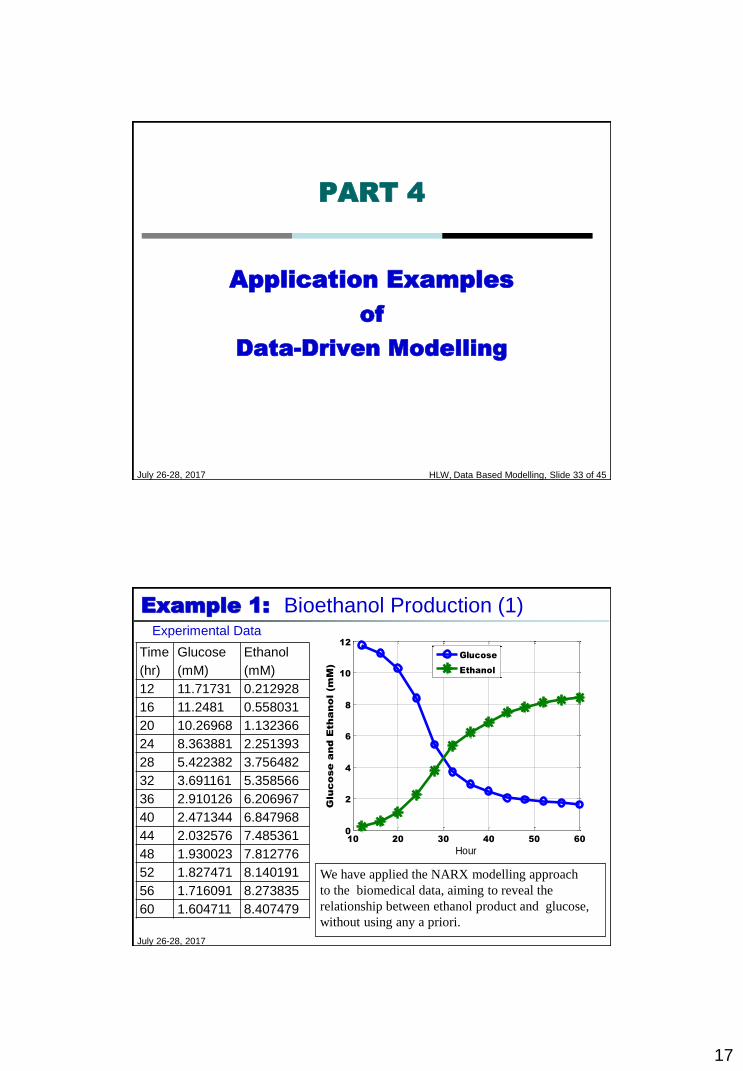
Example 1: Bioethanol Production (1)
Time
(hr)
Glucose
(mM)
Ethanol
(mM)
12 11.71731 0.212928
16 11.2481 0.558031
20 10.26968 1.132366
24 8.363881 2.251393
28 5.422382 3.756482
32 3.691161 5.358566
36 2.910126 6.206967
40 2.471344 6.847968
44 2.032576 7.485361
48 1.930023 7.812776
52 1.827471 8.140191
56 1.716091 8.273835
60 1.604711 8.407479
10 20 30 40 50 600
2
4
6
8
10
12
Hour
Glu
co
se
an
d E
th
an
ol (m
M)
Glucose
Ethanol
We have applied the NARX modelling approach
to the biomedical data, aiming to reveal the
relationship between ethanol product and glucose,
without using any a priori.
Experimental Data
July 26-28, 2017

18
Example 1: Bioethanol Production (2)
The identified NARX Model is
Ethanol(t) = 0.951356×Ethanol(t-1)+0.403146×Glucose(t-2)
– 0.041709×Glucose(t)×Glucose(t-3) + e(t)
10 20 30 40 50 60
0
2
4
6
8
Hour
Eth
an
ol (
mM
)
Measurement
Model prediction
Prediction error
This is a simple
model that can
perfectly link the
system output
(ethonal) to the
input (glucose).
July 26-28, 2017 HLW, Data Based Modelling, Slide 35 of 45
Example 2:
High Tide Forecast at the Venice Lagoon (1)
• A multiscale Cardinal B-spline NARMAX model was
employed
• The identified model was used to predict water levels
of year 1993
• For a case study, the hourly water level data for
year 1992 were used for model estimation
July 26-28, 2017 HLW, Data Based Modelling, Slide 36 of 45

19
Example 3: (cont.)
High Tide Forecast at the Venice Lagoon (2)
0 50 100 150 200-40
-20
0
20
40
60
80
100
120
140
Time [hr]
Wa
ter
Le
vel [
cm]
• 24 hours ahead prediction of water level at the Venice Lagoon in 1993
• Thin solid line: measurements; thick dashed: model prediction
July 26-28, 2017
Example 3: Dst Index Prediction (1)
• Output signaly(t) = Dst(t) (disturbance storm time, [nT]) index
• Input variable
u(t) = VBs(t) (solar wind rectified electric field [mv/m])
• Training data Hourly Dst index and VBs data, March 1-31, 1979
No. of samples = 744
• Test data Hourly Dst index and VBs data, April 1-30, 1979
No. of samples = 720
02486.0)( ty )1(98368.0 ty )1()1(92130.0 3 tuty
)2()3()1(51936.0 2 tutyty )2()1()1(25977.1 2 tututy
• Identified model
July 26-28, 2017 HLW, Data Based Modelling, Slide 38 of 45

20
Example 4: Dst Index Prediction (2)
• Training data: Hourly Dst index and VBs data, March 1-31, 1979 (~ 744)
• Test data: Hourly Dst index and VBs data, April 1-30, 1979 (~ 720)
July 26-28, 2017 HLW, Data Based Modelling, Slide 39 of 45
Example 4: Dst Index Prediction (3)
• Storm 1: PE = 91.48% (PE: Prediction Efficiency)
• Storm 2: PE = 92.17%
• All test data: PE = 93.34%
July 26-28, 2017 HLW, Data Based Modelling, Slide 40 of 45

21
The Understanding of Complex
Systems Needs Data-Driven
Modelling
July 26-28, 2017 HLW, Data Based Modelling, Slide 41 of 45
System Identification Has Many Applications
for the Analysis of Complex Systems
Chertsey BBC, Surry (9.04 am 13th Feb 2014)
In practice, theoretical models are very difficult, if not impossible, to obtain (as they need first principles) . Data-driven modelling provides a complementary but powerful tool for understanding complex systems.
July 26-28, 2017

22
Tips for Data Driven Modelling
and
Concluding Remarks
July 26-28, 2017 HLW, Data Based Modelling, Slide 43 of 45
Tips for Data Driven Modelling
• Always try the simplest possible models first (e.g. linear).
• If a simpler model works, then forget complex models.
• Keep in mind the main purpose of your modelling task.
• Transparent, parsimonious and easily interpretable models
(e.g. regression models) are desirable if you are aiming to reveal dependency and interaction relationships between different explanatory variables/factors.
• If the modelling task is merely focused on prediction or
classification, then either parametric models (e.g. linear regressons) or complicated opaque models (such as ANN models) can be an option.
July 26-28, 2017 Dr HL Wei, Data Based Modelling, Slide 44 of 45

23
Concluding Remarks
• System identification and data driven modelling,
as powerful state-of-the-art approaches, have been widely applied to various areas of science and engineering.
• No particular modelling methods are always the
‘best’ and/or ‘universal’ for all applications, and therefore it is not possible or appropriate to claim that one approach is always better than all the others for solving all problems.
July 26-28, 2017 Dr HL Wei, Data Based Modelling, Slide 45 of 45
Key References1. Wei, H.L., Billings, S.A., & Liu, J. (2004) ‘Term and variable selection for nonlinear system
identification’, International Journal of Control, 77, 86-110.
2. Wei, H.L., Billings, S.A., & Balikhin, M.A. (2004) ‘Prediction of the Dst index using multiresolution wavelet models’ Journal of Geophysical Research, 109, A07212.
3. Wei, H.L., & Billings, S.A. (2006) ‘Long term prediction of nonlinear time series using multiresolution models’, International Journal of Control, 79, 569-580.
4. Wei, H.L., & Billings, S.A. (2006) ‘An efficient nonlinear cardinal B-spline model for high tide forecasts at the Venice Lagoon’, Nonlinear Processes in Geophysics,13,577-584.
5. Wei, H.L., Billings, S.A., & Balikhin, M.A.(2006) ‘Wavelet based nonparametric NARX models for nonlinear input-output system identification’, International Journal of Systems Science, 37(15), 1089-1096.
6. Wei, H.L, Zhu, D., Billings, S.A., & Balikhin, M.A. (2007) ‘Forecasting the geomagnetic activity of the Dst index using multiscale radial basis function networks’, Advances in Space Research, 40, 1863-1870.
7. Billings, S.A., Wei, H.L., & Balikhin, M.A. (2007) ‘Generalised multiscale radial basis function networks’, Neural Networks, 20(10), 1081-1094.
8. Billings, S.A., & Wei, H.L.(2008) ‘An adaptive search algorithm for model subset selection and nonlinear system identification’, International Journal of Control, 81,714-724.
9. Wei, H.L., & Billings, S.A. (2008) ‘Model structure selection using an integrated forward orthogonal search algorithm assisted by squared correlation and mutual information’, International Journal of Modelling, Identification and Control, 3, 341-356.
10. Billings, S.A. (2013) Nonlinear system identification: NARMAX methods in the time, frequency, and spatio-temporal domains: John Wiley & Sons.
11. Ayala Solares, J. R., Wei, H.L., Boynton, R. J., Walker, S. N., & Billings, S. A. (2016) ‘Modelling and Prediction of Global Magnetic Disturbance in Near-Earth Space: a Case Study for Kp Index using NARX Models’, Space Weather, 14(10), 899-916.July 26-28, 2017

24
We gratefully acknowledge that part of this work was supported by:
• EC Horizon 2020 Research and Innovation Action Framework Programme (Grant No 637302 and grant title “PROGRESS”).
• Engineering and Physical Sciences Research Council (EPSRC) (Grant No EP/I011056/1)
• EPSRC Platform Grant (Grant No EP/H00453X/1)
Acknowledgement
July 26-28, 2017
Thank You !Any Questions?
July 26-28, 2017 HLW, Data Based Modelling, Slide 48 of 45