DATA-DRIVEN ENGINEERING OF OPTICAL NETWORKS

by

Steven Santaniello

Copyright © Steven Santaniello 2021

A Report submitted to the Faculty of

COLLEGE OF OPTICAL SCIENCES

In Partial Fulfillment of the Requirements

For the Degree of

MASTER OF SCIENCE

In the Graduate College

THE UNIVERSITY OF ARIZONA

2021

Contents

1 Abstract 3

2 Introduction 4

2.1 Optical Networking and Data . . . . . . . . . . . . . . . . . . 4

2.2 Fiber Transmission . . . . . . . . . . . . . . . . . . . . . . . . 5

2.3 Erbium Doped Fiber Amplifiers . . . . . . . . . . . . . . . . . 7

2.4 Re-configurable Optical Add-Drop Multiplexers . . . . . . . . 8

2.5 Machine Learning and SDN . . . . . . . . . . . . . . . . . . . 11

2.6 Quality of Transmission . . . . . . . . . . . . . . . . . . . . . 13

3 Characterization of SDN Networks 15

3.1 COSMOS Wireless Testbed Overview . . . . . . . . . . . . . . 15

3.2 Characterization of Lumentum ROADM EDFAs . . . . . . . . 16

3.3 Experiemental Setup . . . . . . . . . . . . . . . . . . . . . . . 17

3.3.1 Single Channel Ripple (SCR) . . . . . . . . . . . . . . 18

3.3.2 WDM Ripple . . . . . . . . . . . . . . . . . . . . . . . 19

3.3.3 Individual Channel Loading Configurations . . . . . . . 19

3.4 Single Channel Ripple Characterization . . . . . . . . . . . . . 19

3.5 WDM Ripple Characterization . . . . . . . . . . . . . . . . . . 21

3.6 Individual Channel Configuration Characterization . . . . . . 21

4 Statistical Evaluation 26

4.1 Bayesian Estimation . . . . . . . . . . . . . . . . . . . . . . . 26

1

4.2 Bayesian Estimation of Ripple Fourier Coefficients . . . . . . . 27

4.3 Generation of Random Gain Curves . . . . . . . . . . . . . . . 31

4.4 Limit on Variance . . . . . . . . . . . . . . . . . . . . . . . . . 32

4.5 A Brief Note on Randomized Channel Loading . . . . . . . . . 33

5 Conclusions and Further Research 35

References 37

Appendices 40

A JSON to XLSX Python Scripts 40

2

1 Abstract

The world is becoming increasingly globalized and connected, with the

internet playing the majority role. Today’s internet capabilities are heavily

dependent on optical networking, which uses the properties of light waves to

encode data and send them across cables at the speed of light. The ability

to transmit light at many wavelengths in one fiber, known as Wavelength

Division Multiplexing (WDM), is perhaps the most important enabler of

higher speed and concurrent transmission as more people use the network.

The network usage surge of the COVID-19 pandemic has strained the current

system and highlighted a need to improve network performance evaluation

methods. Fortunately, with the rise of big data, Machine Learning (ML) has

become an attractive and hot topic in handling large amounts of information.

Optical networking is now in a unique situation to employ ML methods

to formulate and understand the customized optical topologies necessary in

modern times. Existing tools, such as the COSMOS testbed in Manhattan,

are a great learning tool that can allow for the collection, interpretation,

and prediction of optical networking performance. These tools, combined

with statistics and data science, will lead into a new generation of optical

networking as the world moves into the virtual age.

3

2 Introduction

The world is increasingly finding itself in a world of big-data, and the

internet is not immune. Between 2005 and 2019, the percentage of the world

population with access to the internet surged from 20% to 50% [1]. This

challenge has only been enhanced by the recent pandemic, which initially

put a strain on telecommunication networks and caused a 38% bandwidth

usage surge from 2019-2020 and a world data transfer rate of around 700

Tbit/s. To handle the high traffic loads, network providers need to be able

to send data more efficiently than they ever have before. The result is a

growing reliance on optical networking.

2.1 Optical Networking and Data

Optical networking involves sending signals encoded in light waves through

free space and optical fibers. The basic concept of this is shown in Figure 1.

An user generates a traffic demand, which is encoded and sent to a transmit-

ter. The transmitter interacts with a laser source to imprint the signal onto

physical properties of the light wave, known as modulation. The encoded

signal is sent via optical fiber to a receiver, which converts the signal back

to the electric domain to interact with the data center’s rack storage. The

request is then processed and data is transmitted back through the network

to the user.

In practice, there is not always a direct link from user straight to the de-

4

sired data source – a signal may need to repeat the process through several

cross-links before reaching the final data center. Thus, the linear transmis-

sion in Figure 1 becomes more of a web, with signals from various sources

traversing the same path between different nodes. As these webs get bigger,

it becomes harder to ensure consistent data transmission in fibers, harder to

distinguish between signals, and harder to handle requests in short amounts

of time. Measurement of signal quality, usually referred to as Quality of

Transmission (QoT), is important in determining how well optical networks

perform. With the rise of on-board optical channel power monitors and other

measurement devices, QoT has the potential to make use of date driven

methods. Fortunately, the parallel development of data science and artificial

intelligence has opened up a breadth of techniques that can be applied to

optical networking to make sense of the data and accelerate network growth.

We will look at several key components in optical networks in subsequent

sections and how the relationship to data can lead to areas of improvement.

2.2 Fiber Transmission

At the heart of any optical communication network is fiber transmis-

sion. The evolution of fiber technology since its inception is 1966 along with

the parallel development in semiconductor lasers has seen data transmission

move from 2.5 Gb/s single channel setups to commercial 400 Gb/s flexible

Wavelength Division Multiplexed (WDM) grids, capable of transmission over

5

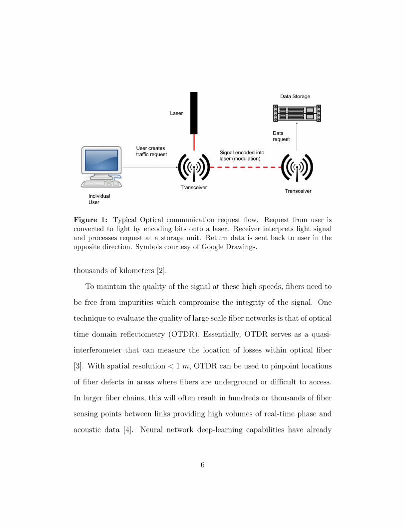
Figure 1: Typical Optical communication request flow. Request from user isconverted to light by encoding bits onto a laser. Receiver interprets light signaland processes request at a storage unit. Return data is sent back to user in theopposite direction. Symbols courtesy of Google Drawings.

thousands of kilometers [2].

To maintain the quality of the signal at these high speeds, fibers need to

be free from impurities which compromise the integrity of the signal. One

technique to evaluate the quality of large scale fiber networks is that of optical

time domain reflectometry (OTDR). Essentially, OTDR serves as a quasi-

interferometer that can measure the location of losses within optical fiber

[3]. With spatial resolution < 1 m, OTDR can be used to pinpoint locations

of fiber defects in areas where fibers are underground or difficult to access.

In larger fiber chains, this will often result in hundreds or thousands of fiber

sensing points between links providing high volumes of real-time phase and

acoustic data [4]. Neural network deep-learning capabilities have already

6

been shown [5] and could easily extend into OTDR sensing of telecom fiber

networks to handle the data loads. By generating neural networks to recover

detailed information, network providers can implement real time monitoring

of large sections of fiber and deploy teams to fix fiber issues with a high degree

of accuracy in the location of the disturbance. Minimizing the complexity

and difficulty of identifying fiber breaks will go a long way in not only network

management, but also identifying better locations for network deployment as

the globe becomes increasingly connected.

2.3 Erbium Doped Fiber Amplifiers

Even with perfect fiber quality, loss is unavoidable in fibers over extremely

large distances as are seen in modern networks. Even though telecom wave-

lengths around 1550 nm minimize fiber loss (Figure 2), a loss of 0.2 dB/km

is detrimental over thousands of kilometers. Erbium Doped Fiber Ampli-

fiers (EDFAs) serve to boost optical signals by sending light through a gain

medium, restoring the signal to desired power levels. Two main types of

EDFAs are relevant to telecom networking – booster amplifiers and pre-

amplifiers. Booster EDFAs increase the optical power before transmission

into a fiber line while pre-amplifiers increase the power of the signal before

entering the optical receiver. In either case, it is essential to understand the

performance of these amplifiers across the bandwidth of interest to optimize

the performance of optical systems.

The gain curve of EDFAs is not typically flat over the entire C-band de-

7

spite having one of the broadest gain spectra in optical amplifiers. Without

uniform gain, signals sent over different wavelengths will experience different

amplification inside the amplifier and have been measured using weak optical

probe sampling [6]. Recently, many EDFA units such as in the Lumentum

ROADM Whitebox 20 have included on-board Optical Channel Monitors

(OCMs) that can measure the channel power directly. With the capacity to

write automated scripts that connect to the on-board channel monitor, a high

volume of data can be obtained for any custom channel loading configuration

using a WSS (see Section 3). A strong characterization of amplifier gains us-

ing real loaded channels can pave the way for Machine Learning techniques

to generate predictions and estimates of amplifier performance based on ex-

perimental data in addition to theoretical considerations. These machine

learning modules could then interact with the next generation of network-

ing emulators such as Mininet Optical [7] and could improve the utility and

cost-saving properties of virtual network test beds.

2.4 Re-configurable Optical Add-Drop Multiplexers

Wavelength Division Multiplexing (WDM) has paved the way for the high

capacity of optical networks. WDM refers to ”bundling” many wavelengths of

light into one stream to be sent through a network simultaneously. Network

providers can thus send dozens of signals together at once through a single

fiber, which not only saves cost but allows for a higher data transfer rate.

Re-configurable add-drop multiplexers (ROADMs) have been established

8

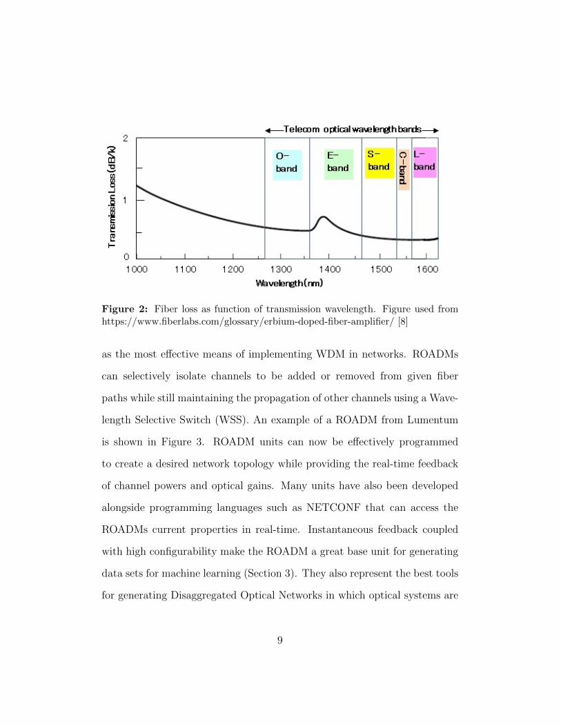
Figure 2: Fiber loss as function of transmission wavelength. Figure used fromhttps://www.fiberlabs.com/glossary/erbium-doped-fiber-amplifier/ [8]

as the most effective means of implementing WDM in networks. ROADMs

can selectively isolate channels to be added or removed from given fiber

paths while still maintaining the propagation of other channels using a Wave-

length Selective Switch (WSS). An example of a ROADM from Lumentum

is shown in Figure 3. ROADM units can now be effectively programmed

to create a desired network topology while providing the real-time feedback

of channel powers and optical gains. Many units have also been developed

alongside programming languages such as NETCONF that can access the

ROADMs current properties in real-time. Instantaneous feedback coupled

with high configurability make the ROADM a great base unit for generating

data sets for machine learning (Section 3). They also represent the best tools

for generating Disaggregated Optical Networks in which optical systems are

9

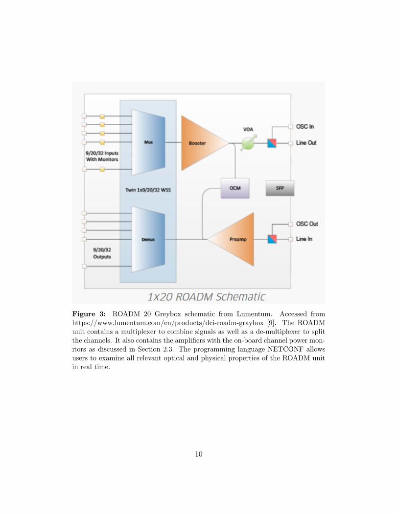
Figure 3: ROADM 20 Greybox schematic from Lumentum. Accessed fromhttps://www.lumentum.com/en/products/dci-roadm-graybox [9]. The ROADMunit contains a multiplexer to combine signals as well as a de-multiplexer to splitthe channels. It also contains the amplifiers with the on-board channel power mon-itors as discussed in Section 2.3. The programming language NETCONF allowsusers to examine all relevant optical and physical properties of the ROADM unitin real time.

10

not designed end to end by single vendors. With devices that can process

multiple network requests from different sources, we can deploy more cost

and space-efficient networks while maintaining the necessary configurability

across multiple users.

ROADM units also make for useful devices in optical testbeds, such as

COSMOS [10]. Testbeds are controlled optical networks that are created to

emulate an actual deployed network in local settings. The high degree of flex-

ibility in channel configurations that ROADMs can create along with a WSS

and a variable laser source can allow researchers to configure many optical

topologies in seconds. Testbeds provide a better way to test hypotheses and

strategies in optical networking, as equipment is very expensive and difficult

to implement quickly. It also provides a controlled setting with streamlined

data collection to allow for rigorous testing and implementation of SDN con-

trol planes.

2.5 Machine Learning and SDN

A growing subject in the realm of optical networking is machine learn-

ing and AI-based data analysis methods. Part of the motivation for this

deals with network reconfiguration – demands on the network can often

change rapidly, while the actual reconfiguration of the network takes much

longer. Predicting these changes proactively is nearly impossible for a net-

work provider, hence motivating the need for automated and smart solutions.

The key foundation of machine learning in networking is known as Soft-

11

ware Defined Networking (SDN). In brief, SDN separates the control plane

from the physical data plane that forwards network traffic [11]. Before SDN,

everything was managed and controlled at the hardware level. SDN brings

virtualization to the network and centralizes the control flow away from in-

dividual network elements [12]. Using protocols such as OpenFlow, network

managers have software access to flow tables that can forward changes to the

physical layer to manage traffic. As the internet moves towards a data-driven

approach, SDN will enable the transition between legacy networks and the

abstract virtual networks of the future.

Even with its utility, SDN still may have trouble with the high growth

of internet usage (Section 2) and the high increase of high data applications

such as big data and video streams. This is where Machine Learning (ML) is

applicable. The union of SDN and ML is sometimes referred to as a Knowl-

edge Based Network (KDN). Machine learning algorithms, and by extension

KDN, are highly dependent on the training data set used to inform the ML

as well as the predictive ability of generated Machine Learning classifiers. In

this way, many have focused their research into identifying classifiers that

hold high predictive merit [13]. For example, the most misclassified group

of light channels might be in the ”minority group”, which will not show a

large drop in classification accuracy percentages overall. Receiver operating

characteristic curves, or ROC curves, can help to identify the frequency of

specific types of errors and help to understand which light channels are actu-

ally ”bad” and need to be reconfigured. ROC curves show the performance

12

of binary classifiers, such as determining good vs. bad optical channels, as

discrimination thresholds are varied. KDN will always have a constant battle

with creating classifiers that over-fit the training data, meaning that classi-

fiers also need to evaluated with ROC as well as regression tests to evaluate

the practicality of the design in implementation.

A promising subset of ML in end-to-end transmission system design is

that of deep neural networks. For instance, a recent paper has showcased

speeds of 42 Gb/s over 40 km of transmission and as high as 84 Gb/s over

20 km while staying below the hard-decision forward error correction coding

limit [14]. This concept of layered algorithms can help network providers

to extract anything from low-level values such as optical power to higher-

level, more complex terms such as gOSNR. These terms are associated with

the topic of quality of transmission (QoT), which is the subject of the next

section.

2.6 Quality of Transmission

QoT is a wide-ranging term used to describe the quality of optical signals

in optical networks. In simple end-to-end systems, this is relatively straight

forward as signal to noise ratio (SNR) and bit-error rates (BER) directly

correspond to the quality of the signal. However, in the dynamic and cloud-

based networks of today, QoT is a complex phenomenon that often requires

multiple levels of analysis. These figures of merit can be calculated across

all possible optical paths in a network, which grow exponentially with more

13

nodes. As DWDM backbone workloads increase, QoT becomes a global prob-

lem rather than simply a local measurement. This section aims to explore

some machine learning methods dealing with QoT.

Machine learning problems revolve around finding generalized, efficient

classifiers from a set of quality training data. Since changes to a SDN net-

work come from the control plane, the data used to make ML predictions

including those about QoT need to come only from data accessible to the

control plane [13]. A proper flow of information from network element reports

to controlled data structures and then to a defined ML database typically

represents how training sets are built. For example, hops in an optical path

as well as losses in dB may be recorded in hardware specific data structures,

and SDN planes will need to convert the formatting and store it in an appro-

priate database. Choice of relevant data is dependent on the purpose, but

QoT often references power and noise measurements. Once data is compiled,

ML algorithms employ statistical strategies to determine ”good” and ”bad”

channels. One such example is Logistic Regression which forms the proba-

bilistic backbone of support vector machines and operates as a linear binary

classifier. Other options available for analyzing tabular data include gradient

boosting and random forests which represent ensemble data modeling. This

is beyond the scope of this report, although some important statistical con-

cepts related to these algorithms will be explored in Section 4 with Bayesian

recursion.

14

3 Characterization of SDN Networks

Section 2 surveyed current literature about the current state and future

goals of SDN network evaluation. In this section, a real-life example will

be explored with the COSMOS (Cloud Enhanced Open Software Defined

Mobile Wireless Testbed for City-Scale Deployment) Testbed.

3.1 COSMOS Wireless Testbed Overview

COSMOS, located in upper Manhattan, is designed to provide real-world

experimental capabilities on a city-scale configurable optical network (Fig-

ure 4). The central Calient Switch allows researchers to send optical signals

with up to 95 independent wavelength channels across a configurable net-

work operated by an SDN controller. Experimenters then have full access

to all network data and can monitor in real time the performance of desired

optical topologies. An example of a programmable optical topology is given

in Figure 6. The core of the network consists of the programmable Calient

switch, connected fiber spools, and 6 available ROADM units. As we will

see in Section 3.2, the comb source can use a WSS to generate the 95 optical

channels which can be sent through the Calient to ROADM amplifiers to

characterize their performance. COSMOS is thus a convenient and useful

option for testing the real-world performance of networking controllers and

components simultaneously.

15

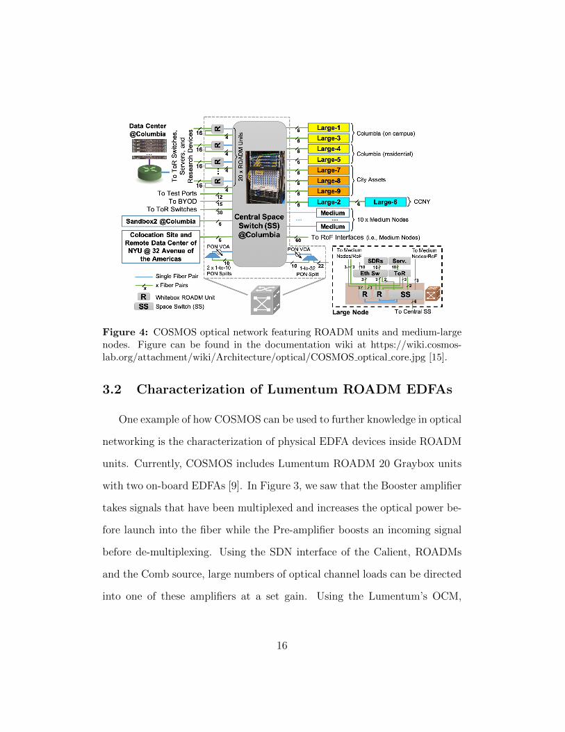
Figure 4: COSMOS optical network featuring ROADM units and medium-largenodes. Figure can be found in the documentation wiki at https://wiki.cosmos-lab.org/attachment/wiki/Architecture/optical/COSMOS optical core.jpg [15].

3.2 Characterization of Lumentum ROADM EDFAs

One example of how COSMOS can be used to further knowledge in optical

networking is the characterization of physical EDFA devices inside ROADM

units. Currently, COSMOS includes Lumentum ROADM 20 Graybox units

with two on-board EDFAs [9]. In Figure 3, we saw that the Booster amplifier

takes signals that have been multiplexed and increases the optical power be-

fore launch into the fiber while the Pre-amplifier boosts an incoming signal

before de-multiplexing. Using the SDN interface of the Calient, ROADMs

and the Comb source, large numbers of optical channel loads can be directed

into one of these amplifiers at a set gain. Using the Lumentum’s OCM,

16

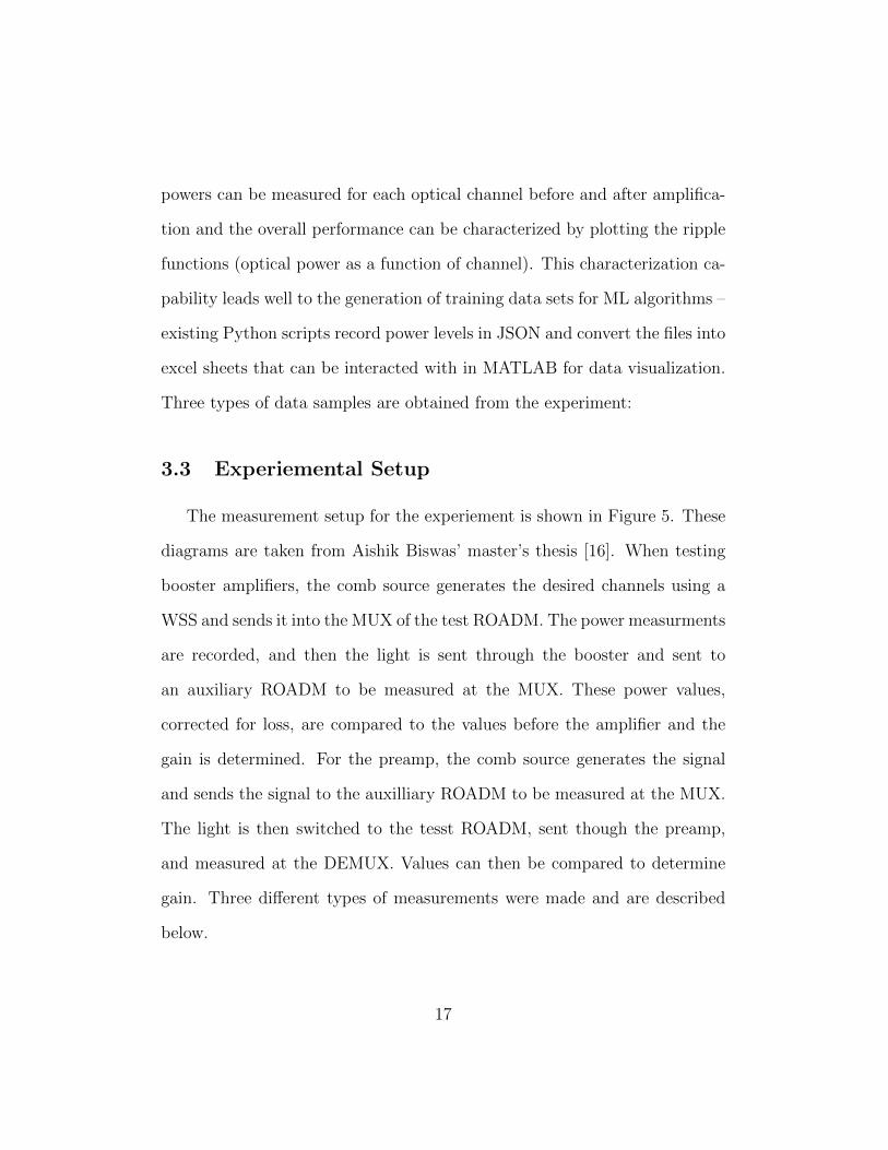
powers can be measured for each optical channel before and after amplifica-

tion and the overall performance can be characterized by plotting the ripple

functions (optical power as a function of channel). This characterization ca-

pability leads well to the generation of training data sets for ML algorithms –

existing Python scripts record power levels in JSON and convert the files into

excel sheets that can be interacted with in MATLAB for data visualization.

Three types of data samples are obtained from the experiment:

3.3 Experiemental Setup

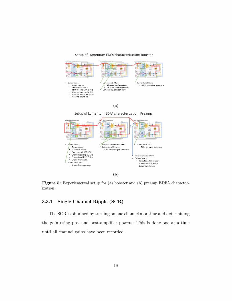
The measurement setup for the experiement is shown in Figure 5. These

diagrams are taken from Aishik Biswas’ master’s thesis [16]. When testing

booster amplifiers, the comb source generates the desired channels using a

WSS and sends it into the MUX of the test ROADM. The power measurments

are recorded, and then the light is sent through the booster and sent to

an auxiliary ROADM to be measured at the MUX. These power values,

corrected for loss, are compared to the values before the amplifier and the

gain is determined. For the preamp, the comb source generates the signal

and sends the signal to the auxilliary ROADM to be measured at the MUX.

The light is then switched to the tesst ROADM, sent though the preamp,

and measured at the DEMUX. Values can then be compared to determine

gain. Three different types of measurements were made and are described

below.

17

(a)

(b)

Figure 5: Experiemental setup for (a) booster and (b) preamp EDFA character-ization.

3.3.1 Single Channel Ripple (SCR)

The SCR is obtained by turning on one channel at a time and determining

the gain using pre- and post-amplifier powers. This is done one at a time

until all channel gains have been recorded.

18

3.3.2 WDM Ripple

Similar to the SCR, the WDM ripple uses pre- and post-amplifier powers

to determine channel gain through the amplifier, but this time it is done all

at once by turning on all channels and recording the powers simultaneously.

3.3.3 Individual Channel Loading Configurations

Most of the samples obtained from the experiments are randomized chan-

nel loading configuration power curves. These are obtained by generating a

list of 2-10 channels to turn on and measuring the output power of all channels

post-amplifier. We will examine the statistical reasoning behind stopping at

10 channels in Section 4. The result is a mostly flat power curve with the

activated channels showing peaks corresponding to the set gain values. We

will now look at some sample data in detail.

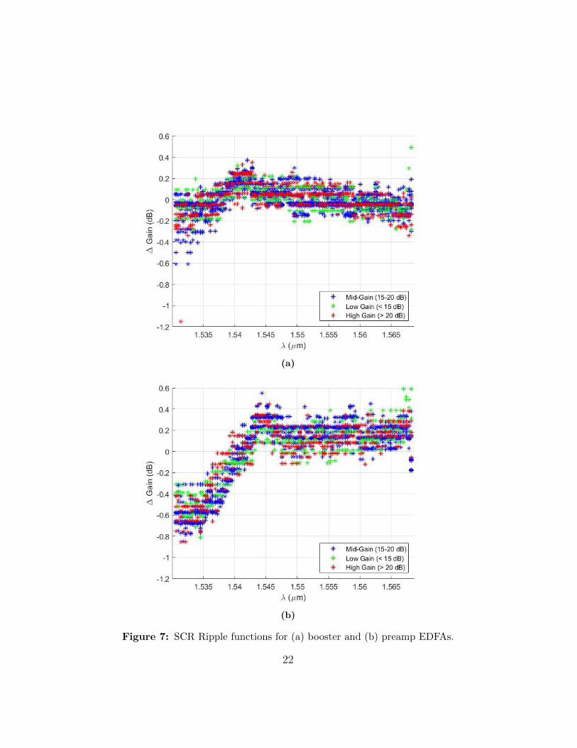
3.4 Single Channel Ripple Characterization

The term ”Single Channel Ripple” refers to gain measurements taken by

activating one channel, recording the power before and after the amplifier,

and turning it off again before moving to the next channel. The result is a

gain measurement for each of the 95 channels. To find the SCR function, the

mean gain is calculated and subtracted from the channel gain measurement:

∆Gi = Gi −1

n

95∑i=1

Gi (1)

19

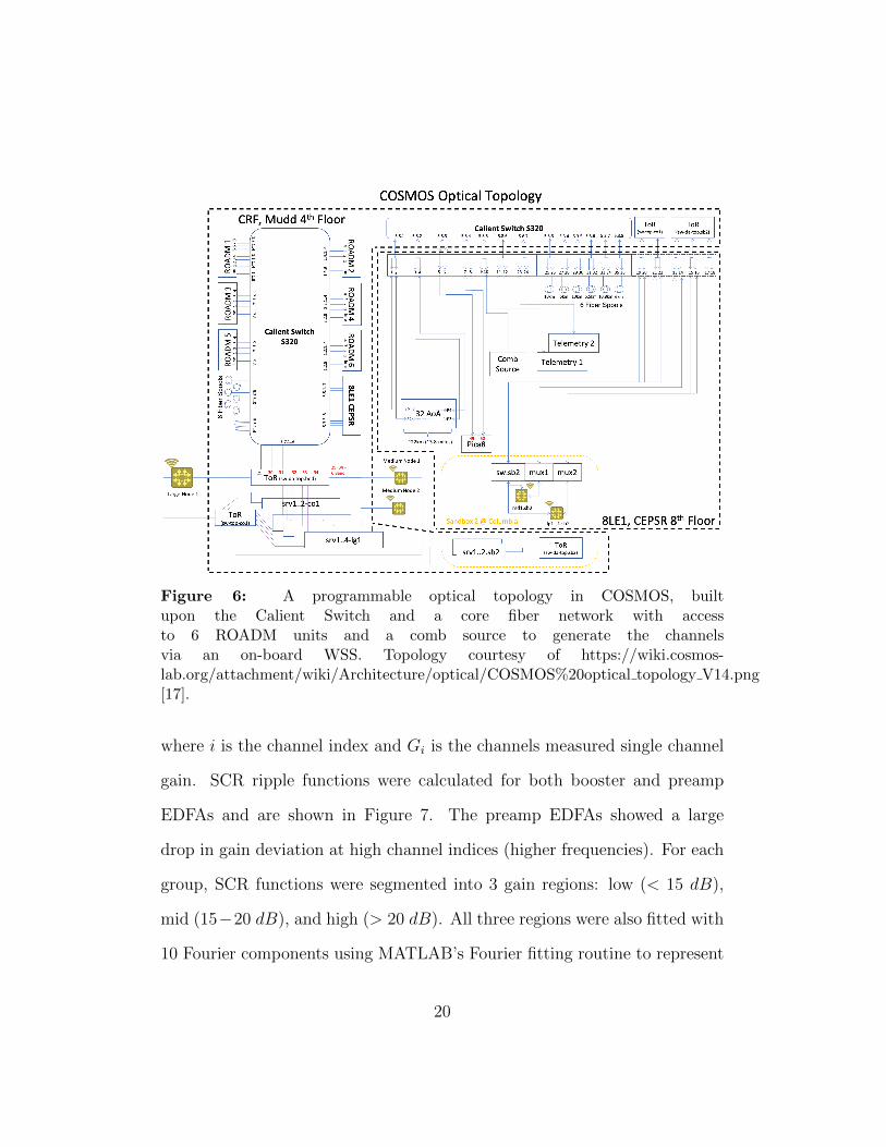
Figure 6: A programmable optical topology in COSMOS, builtupon the Calient Switch and a core fiber network with accessto 6 ROADM units and a comb source to generate the channelsvia an on-board WSS. Topology courtesy of https://wiki.cosmos-lab.org/attachment/wiki/Architecture/optical/COSMOS%20optical topology V14.png[17].

where i is the channel index and Gi is the channels measured single channel

gain. SCR ripple functions were calculated for both booster and preamp

EDFAs and are shown in Figure 7. The preamp EDFAs showed a large

drop in gain deviation at high channel indices (higher frequencies). For each

group, SCR functions were segmented into 3 gain regions: low (< 15 dB),

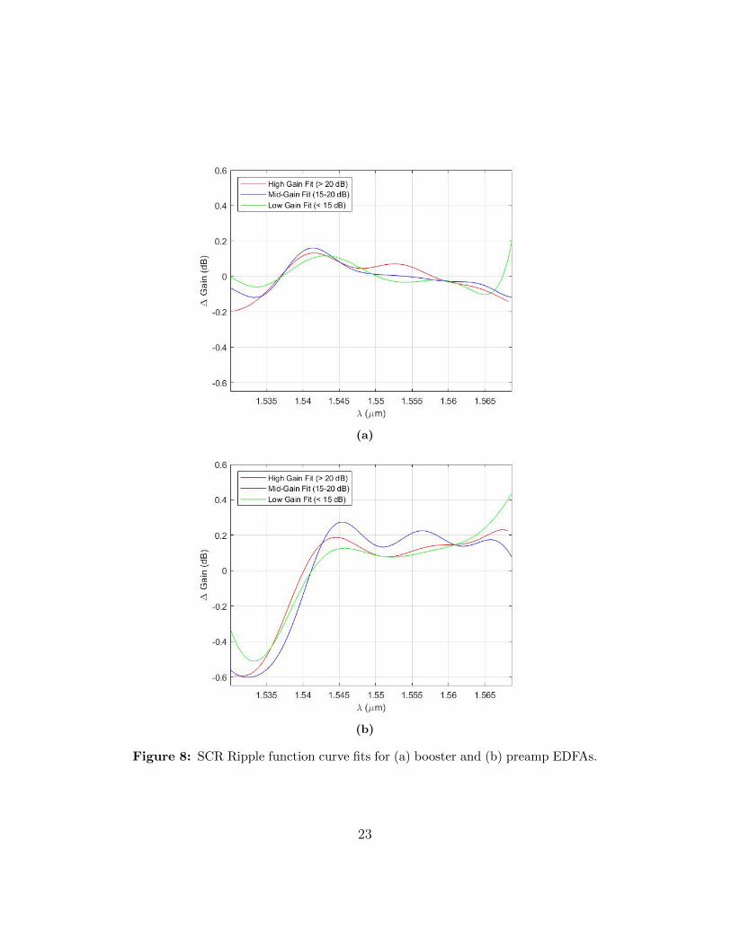
mid (15−20 dB), and high (> 20 dB). All three regions were also fitted with

10 Fourier components using MATLAB’s Fourier fitting routine to represent

20

the data as a Fourier series:

FG = a0 +4∑i=1

ai cos(ixω) + bi sin(ixω) (2)

In Section 4, we will develop a probability distribution for these coefficients

using an empirical prior distribution and Bayesian Recursion to refine the

posterior distribution. The results of the fittings are shown in Figure 8.

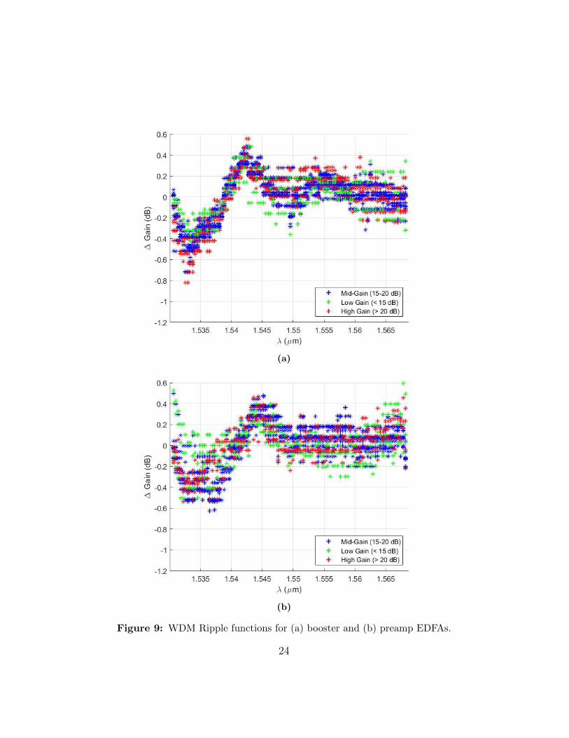
3.5 WDM Ripple Characterization

The WDM ripple function is related to the SCR, but instead of turning

on and measuring one channel at a time, all 95 channels are activated and

measured at the same time. The results from the same test samples as

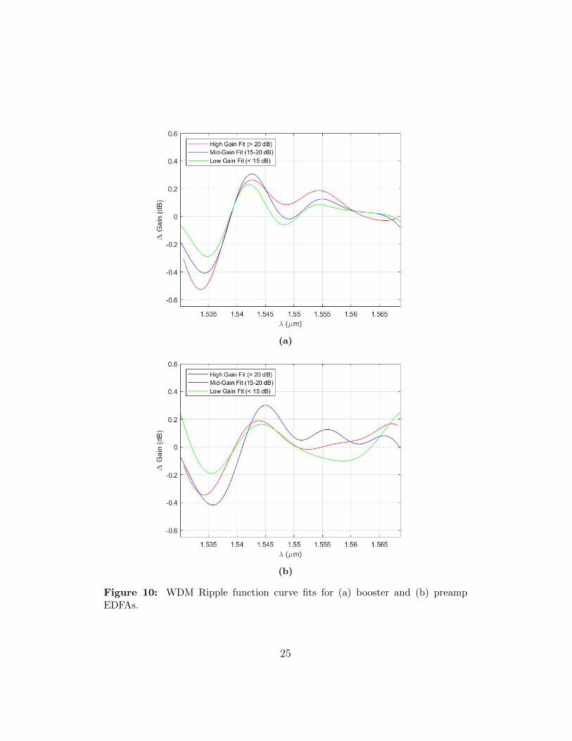
Section 3.3 are shown in Figure 9. Fourier fits to the data are also shown

in Figure 10. An interesting trend with the WDM ripple as opposed to the

SCR function is that the Fourier fits of the booster and preamplifier EDFAs

exhibit a more similar behavior to each other. This is because of the tendency

of EDFA gain curves to ”saturate” and resemble a universal WDM curve as

many channels are activated. In other words, individual characteristics and

wavelength dependent gain have less effect as many channels are activated.

3.6 Individual Channel Configuration Characterization

With each amplifier test, 3600 samples of individual random loading con-

figurations are recorded and stored for training purposes. More work needs

21

(a)

(b)

Figure 7: SCR Ripple functions for (a) booster and (b) preamp EDFAs.

22

(a)

(b)

Figure 8: SCR Ripple function curve fits for (a) booster and (b) preamp EDFAs.

23

(a)

(b)

Figure 9: WDM Ripple functions for (a) booster and (b) preamp EDFAs.

24

(a)

(b)

Figure 10: WDM Ripple function curve fits for (a) booster and (b) preampEDFAs.

25

to be done to characterize these samples and to examine their significance in

finding outlier cases.

4 Statistical Evaluation

In Section 3, three types of data were reported. The goal of this section

is to attempt to describe statistically the significance of the EDFA tests and

to present a method for deriving a probability distribution. The concept of

Bayesian Estimation will be used on the Fourier coefficients for the ripple

functions, and will be introduced here.

4.1 Bayesian Estimation

A common goal in statistics is to use an obtained sample to gain inference

about unknown parameters. Classical approaches to statistics often assume

the unknown parameter θ is fixed, and the sample will give us a range of

plausible values that θ might take. In Bayesian estimation, the approach

is slightly different and resembles Bayes’ Rule [18]. The parameter θ is as-

sumed to vary according to a distribution π(θ), and is known as the prior

distribution. The prior distribution is based on prior knowledge and is for-

mulated prior to the sample being taken. Common methods for forming a

prior distribution range from experimental beliefs held by the investigator to

an empirical distribution formed from previous experiments. Once a sample

X1...Xn is taken, the prior distribution is updated with the knowledge of the

26

sample by:

π(θ|x) =f(x|θ) π(θ)

m(x)(3)

Where f(x|θ) π(x) is the joint distribution of the sample and the prior dis-

tribution and m(x) is the marginal distribution of the sample found by:

m(x) =∫f(x|θ)π(x) dθ (4)

In this sense, the distribution that estimates θ can be continually updated

using the distribution of incoming samples. An important assumption that

simplifies the computation of m(x) is the independence of the prior and the

conditional distribution. Since π(θ) is developed independent of future sam-

ples and the samples of EDFA data are taken as independent measurements,

we will assume this condition is satisfied. The benefits of this approach is

that the posterior distribution can become a prior distribution in further

testing, and the distribution describing ripple function Fourier coefficients

can be refined with further testing.

4.2 Bayesian Estimation of Ripple Fourier Coefficients

Based on the lack of existing data on Fourier fitting of ripple functions,

we will attempt Bayesian Recursion using empirical data for booster ampli-

fiers. In the data set under study, there are 24 measurements of 10 Fourier

coefficients that describe the ripple function. We will use the first 5 tests to

generate the prior distribution for each coefficient. Also, due to the lack of

27

µ σa0 -0.0961 1.5638a1 0.0473 2.2449b1 -0.3711 1.5599a2 0.3414 0.7298b2 -0.2699 1.6097a3 0.3229 0.3216b3 -0.0119 0.7442a4 0.1069 0.1605b4 0.0282 0.1379w 5.12 e-11 1.12 e-10

Table 1: Empirical mean and standard deviation of normal prior distribution forripple fit coefficients.

data, a nominal place to start is to estimate each distribution as a normal

distribution:

π(θ) =1√2πσ

exp(−1

2σ2(x− µ)2

)(5)

Using the initial 5 samples, ten normal distributions describing a0...b4 were

formulated using MATLAB’s normfit function, generating a µ and σ for

each coefficient. The results of the empirical fitting are shown in Table 1.

For example, the coefficient a0 has the values of µ = −0.0096 and σ = 1.564,

meaning the distribution of a0 is the normal distribution shown in Figure

11. Now that we have fit a prior distribution, we can ”update” it with the

rest of the samples to see if the normal distribution holds to more samples.

For the rest of the samples, the distribution fit to the coefficients was no

longer constrained to a normal distribution, but turned out to be the best

fit in all cases. This result draws an interesting parallel between the concept

28

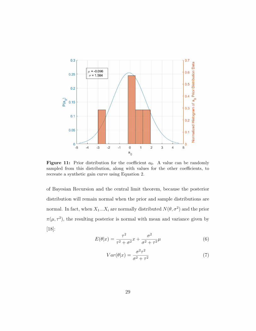
Figure 11: Prior distribution for the coefficient a0. A value can be randomlysampled from this distribution, along with values for the other coefficients, torecreate a synthetic gain curve using Equation 2.

of Bayesian Recursion and the central limit theorem, because the posterior

distribution will remain normal when the prior and sample distributions are

normal. In fact, when X1...Xi are normally distributed N(θ, σ2) and the prior

π(µ, τ 2), the resulting posterior is normal with mean and variance given by

[18]:

E(θ|x) =τ 2

τ 2 + σ2x+

σ2

σ2 + τ 2µ (6)

V ar(θ|x) =σ2τ 2

σ2 + τ 2(7)

29

µ σa0 0.0093 1.5563a1 0.0024 2.2206b1 0.1377 1.5549a2 0.1166 0.7270b2 0.0729 1.597a3 0.1043 0.3204b3 7.65 e-4 0.7266a4 0.0138 0.1381b4 8.13 e-4 0.1364w 6.68 e-13 8.84 e-13

Table 2: Posterior fourier coefficient mean and standard deviation. All parame-ters apply to a normal distribution.

The new parameters of the final posterior distribution are shown in Table

2. Only two coefficients, b3 and w, had a strong enough dependence on x

to need it for a good approximation of E(θ|x). The other coefficients had

τ2

τ2+σ2 = 10−5 or lower and thus E(θ|x) was dominated by the term depending

on µ. To determine the final values in the table, another test was used to

simplify the b3 and w expressions.

It is natural to wonder if the results of the Bayesian method has advan-

tages over the conventional method of statistics. Looking at Equations 6 and

7, we can see that the results for E(θ|x) and V ar(θ|x) depend heavily on the

variances of the prior and sample distributions. When σ >> τ , more weight

is given to prior distribution, whereas when τ >> σ, the sample gets more

weight. In the case shown here, the incoming sample variance was much

higher than that of the prior, so not a lot of change occurred from prior to

posterior. However, if we had chosen 5 samples with a higher variance, then

30

the sample would have had more weight and a larger change in expectation

would occur. The classical framework of statistics does not allow as much

flexibility to incoming samples, and this Bayesian framework will allow the

distribution to be refined with further testing.

4.3 Generation of Random Gain Curves

The goal of generating the distribution for Fourier fitting coefficients was

to be able to generate random realistic curves that resemble real gain ripples.

Now that each Fourier coefficient was modeled by a distribution of the form

in Equation (2), we are able to create synthetic distributions across our

channel spectrum. The results of 5 randomly generated curves are shown

in Figure 12. The deviation ∆ Gain is an order of magnitude higher than

expected from the sample data in Section 3. As we know from statistics,

independent draws from normal distributions lead to a normal distribution

with a variance scaled by 1/n. As more samples are considered, the variance

of the distribution is likely to decrease proportionally to this factor. 5 random

curves generated with 1/10 of the variance of Bayesian estimation lead to the

curves shown in Figure 13. These curves now have a more realistic value for

∆ Gain and exhibit more similar behavior to each other. As more samples

are collected, this Bayesian framework should allow for increasingly more

accurate representations of real gain curves and more relevant uses of Data

Augmentation, which can help create useful machine learning test cases from

artificial data.

31

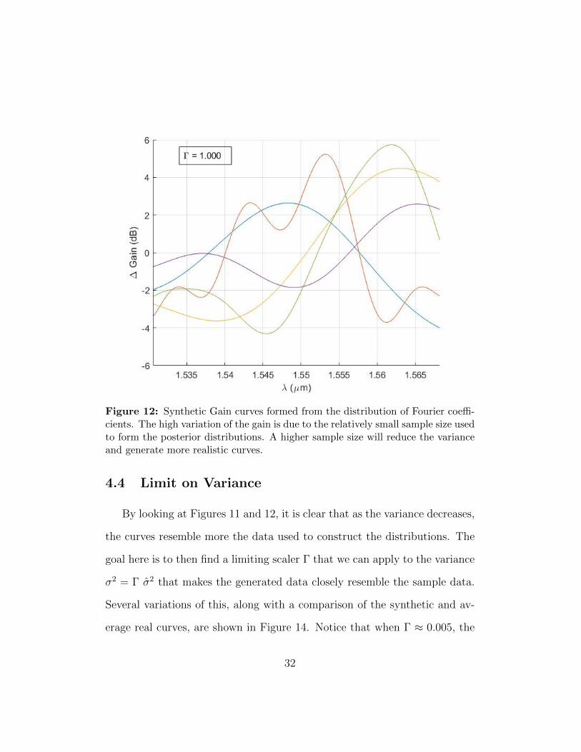
Figure 12: Synthetic Gain curves formed from the distribution of Fourier coeffi-cients. The high variation of the gain is due to the relatively small sample size usedto form the posterior distributions. A higher sample size will reduce the varianceand generate more realistic curves.

4.4 Limit on Variance

By looking at Figures 11 and 12, it is clear that as the variance decreases,

the curves resemble more the data used to construct the distributions. The

goal here is to then find a limiting scaler Γ that we can apply to the variance

σ2 = Γ σ2 that makes the generated data closely resemble the sample data.

Several variations of this, along with a comparison of the synthetic and av-

erage real curves, are shown in Figure 14. Notice that when Γ ≈ 0.005, the

32

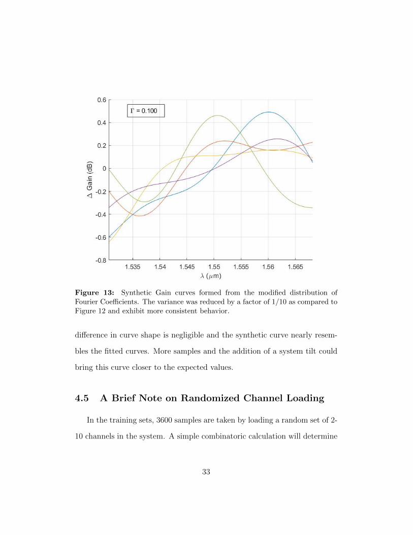
Figure 13: Synthetic Gain curves formed from the modified distribution ofFourier Coefficients. The variance was reduced by a factor of 1/10 as compared toFigure 12 and exhibit more consistent behavior.

difference in curve shape is negligible and the synthetic curve nearly resem-

bles the fitted curves. More samples and the addition of a system tilt could

bring this curve closer to the expected values.

4.5 A Brief Note on Randomized Channel Loading

In the training sets, 3600 samples are taken by loading a random set of 2-

10 channels in the system. A simple combinatoric calculation will determine

33

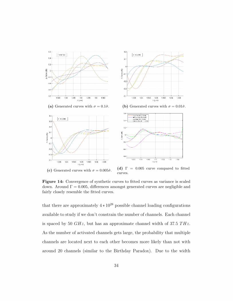
(a) Generated curves with σ = 0.1σ. (b) Generated curves with σ = 0.01σ.

(c) Generated curves with σ = 0.005σ.(d) Γ = 0.005 curve compared to fittedcurves.

Figure 14: Convergence of synthetic curves to fitted curves as variance is scaleddown. Around Γ = 0.005, differences amongst generated curves are negligible andfairly closely resemble the fitted curves.

that there are approximately 4 ∗ 1028 possible channel loading configurations

available to study if we don’t constrain the number of channels. Each channel

is spaced by 50 GHz, but has an approximate channel width of 37.5 THz.

As the number of activated channels gets large, the probability that multiple

channels are located next to each other becomes more likely than not with

around 20 channels (similar to the Birthday Paradox). Due to the width

34

of the channel and the limited channel parameter space, the ripple function

will begin to wash out over time and tend to the WDM case as the noise

bleeds in to ”off” channels. Studying the region of 2-10 channels allows for

edge cases to be considered while these pseudo-WDM ripple cases can be

ignored, allowing the parameter space to be reduced by at least 14 orders of

magnitude. As more is discovered about how edge-case loading configurations

affect amplifier performance, there should be a volume of data to support ML

correcting methods in unique channel loading cases.

5 Conclusions and Further Research

The world of ML and optical networking are becoming increasingly con-

nected as demands on DWDM backbones increase. The growing size of

networks and the rapid increase in customized optical topologies continue

to make QoT estimation a difficult and complex challenge. The COSMOS

optical testbed provides us with a unique opportunity to test artificial intel-

ligence methods and develop strategies to predict the performance of optical

networks. As we have seen in Sections 3 and 4, there is an ample amount of

data available about the optical components in COSMOS and some useful

insights about potential roadblocks that can be encountered. As COSMOS

expands, more experimentation is in planning which will allow us to compare

the use of a new class of optical testbeds – virtual simulators and emulators,

such as Mininet optical. Mininet will allow researchers to generate their own

35

optical networks in a virtual machine environment and test experimental sce-

narios without the financial resource investment in expensive hardware. As

optical networking moves towards its own data revolution, tools like COS-

MOS, Mininet, and ML QoT estimation will lead the way in ensuring network

providers are able to meet the demands of an interconnected world.

36

References

[1] I. T. Union, “Measuring digital development facts and figures 2020,”

Place des Nations 1211 Geneva 20 Switzerland, 2020. [Online]. Avail-

able: https://www.itu.int/en/ITU-D/Statistics/Documents/

facts/FactsFigures2020.pdf.

[2] X. Liu, “Evolution of fiber-optic transmission and networking toward

the 5g era,” iScience, vol. 22, pp. 489–506, 2019. doi: https://doi.

org/10.1016/j.isci.2019.11.026.

[3] S. V. Shatalin, V. N. Treschikov, and A. J. Rogers, “Interferometric op-

tical time-domain reflectometry for distributed optical-fiber sensing,”

Applied Optics, vol. 37, no. 24, 1998. doi: http://dx.doi.org/10.

1364/AO.37.005600.

[4] P. Westbrook, “Big data on the horizon from a new generation of dis-

tributed optical fiber sensors,” APL Photonics, vol. 5, no. 2, p. 020 401,

2020. doi: https://doi.org/10.1063/1.5144123.

[5] A. Sinha, J. Lee, S. Li, and G. Barbastathis, “Lensless computational

imaging through deep learning,” Optica, vol. 4, pp. 1117–1125, 9 2017.

doi: https://doi.org/10.1364/OPTICA.4.001117.

[6] W. Mo, S. Zhu, Y. Li, and D. C. Kilper, “Edfa wavelength dependent

gain spectrum measurement using weak optical probe sampling,” IEEE

Photonics Technology Letters, vol. 30, pp. 177–180, 2 2017. doi: https:

//doi.org/10.1109/LPT.2017.2779746.

37

[7] B. Lantz, A. A. Dıaz-Montiel, J. Yu, C. Rios, M. Ruffini, and D. Kilper,

“Demonstration of software-defined packet-optical network emulation

with mininet-optical and onos,” in 2020 Optical Fiber Communications

Conference and Exhibition (OFC), 2020, pp. 1–3.

[8] F. L. Inc., Erbium-doped fiber amplifier (edfa). [Online]. Available:

https://www.fiberlabs.com/glossary/erbium- doped- fiber-

amplifier/, (accessed: 03.28.2021).

[9] L. O. LLC, Roadm graybox. [Online]. Available: https://www.lumentum.

com/en/products/dci-roadm-graybox, (accessed: 03.28.2021).

[10] Cosmos. [Online]. Available: https://www.cosmos-lab.org/.

[11] M. Cooney, What is sdn and where software-defined networking is go-

ing, Apr. 2019. [Online]. Available: https://www.networkworld.com/

article/3209131/what- sdn- is- and- where- its- going.html,

(accessed: 03.28.2021).

[12] M. Jammal, T. Singh, A. Shami, R. Asal, and Y. Li, “Software de-

fined networking: State of the art and research challenges,” Computer

Networks, vol. 72, May 2014. doi: 10.1016/j.comnet.2014.07.004.

[13] S. Kozdrowski, P. Cichosz, P. Paziewski, and S. Sujecki, “Machine

learning algorithms for prediction of the quality of transmission in opti-

cal networks,” Entropy, vol. 23, no. 1, 2021. doi: 10.3390/e23010007.

38

[14] B. Karanov, M. Chagnon, F. Thouin, T. A. Eriksson, H. Bulow, D.

Lavery, P. Bayvel, and L. Schmalen, “End-to-end deep learning of op-

tical fiber communications,” Journal of Lightwave Technology, vol. 36,

no. 20, pp. 4843–4855, 2018. doi: 10.1109/JLT.2018.2865109.

[15] [Online]. Available: https://wiki.cosmos-lab.org/attachment/

wiki/Architecture/optical/COSMOS%5C_optical%5C_core.jpg.

[16] A. Biswas, “Telemetry and data collection for artificial intelligence

in optical systems,” M.S. thesis, 2020. [Online]. Available: https://

repository.arizona.edu/handle/10150/645778.

[17] [Online]. Available: https://wiki.cosmos-lab.org/attachment/

wiki/Architecture/optical/COSMOS%5C%20optical%5C_topology%

5C_V14.png.

[18] G. Casella and R. L. Berger, Statistical Inference. 511 Forest Lodge

Road Pacific Grove, CA 93950: Duxbury, 2002.

39

Appendices

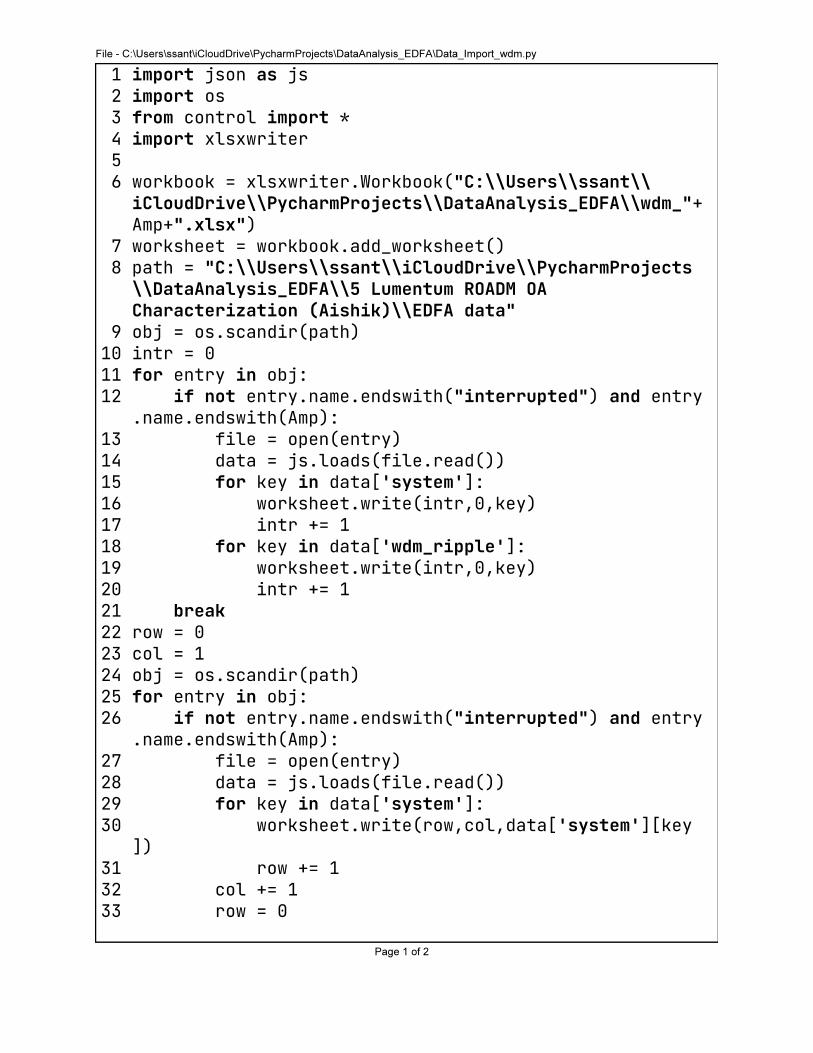
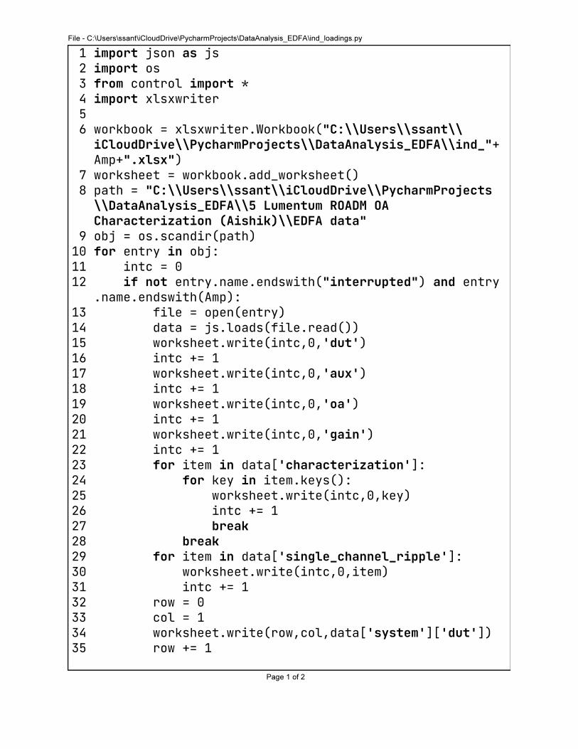
A JSON to XLSX Python Scripts

The following scripts were written to take EDFA data from the extraction

scripts and convert it from JSON format in an XLSX file to be easily worked

with in MATLAB.

40