1

DATA COMMUNICATIONS

&

COMPUTER NETWORK

LECTURE NOTES

By R.P.Nayak

Department of Computer Science and Engineering, Kalahandi,

Bhawanipatna 766002

2

Course of Studies

Module – I (12 Hrs) Overview of Data Communications and Networking. Physical Layer : Analog and Digital, Analog Signals, Digital Signals, Analog versus Digital, Data Rate Limits, Transmission Impairment, More about signals. Digital Transmission: Line coding, Block coding, Sampling, Transmission mode. Analog Transmission: Modulation of Digital Data; Telephone modems, modulation of Analog signals. Multiplexing : FDM , WDM , TDM. Transmission Media: Guided Media, Unguided Media (wireless). Circuit switching and Telephone Network: Circuit switching, Telephone network.

Module –II (12 Hrs) Data Link Layer Error Detection and Correction: Types of Errors, Detection, Error Correction Data Link Control and Protocols: Flow and Error Control, Stop-and-wait ARQ. Go-Back-N ARQ, Selective Repeat ARQ, HDLC. Point-to –Point Access: PPP ,Point –to- Point Protocol, PPP Stack, Multiple Access: Random Access, Controlled Access, Channelization. Local area Network: Ethernet, Traditional Ethernet, Fast Ethernet, Gigabit Ethernet. Token bus, Token ring. Wireless LANs: IEEE 802.11, Bluetooth Virtual Circuits: Frame Relay and ATM. Module – III (12 Hrs) Network Layer: Host to Host Delivery: Internetworking, addressing and Routing. Network Layer Protocols: ARP, IPV4, ICMP, IPV6 and ICMPV6. Transport Layer: Process to Process Delivery: UDP, TCP, Congestion Control and Quality of Service. Application Layer : Client Server Model, Socket Interface, Domain Name System (DNS), Electronic Mail (SMTP) and File Transfer (FTP), HTTP and WWW. Text Books: 1. Data Communications and Networking: Behrouz A. Forouzan, Tata McGraw-Hill, 4

th Ed

2. Computer Networks: A. S. Tannenbum, D. Wetherall, Prentice Hall, Imprint of Pearson 5th

Ed Reference Book : . 1. Computer Networks:A system Approach:Larry L, Peterson and Bruce S.

Davie,Elsevier, 4th

Ed 2. Computer Networks: Natalia Olifer, Victor Olifer, Willey India 3. Data and Computer Communications: William Stallings, Prentice Hall, Imprint of

Pearson, 9th

Ed. 4. Data communication & Computer Networks: Gupta, Prentice Hall of India 5. Network for Computer Scientists & Engineers: Zheng, Oxford University Press 6. Data Communications and Networking: White, Cengage Learning

3

Module -i & Module-ii Important topics discussed:

1. Components of Data communication 2. Network physical structures 3. Network models 4. OSI Model 5. TCP/IP protocol 6. Different types of addresses 7. Nyquist bit rate 8. Shannon Capacity 9. PCM 10. Transmission modes 11. Manchester and Differential Manchester 12. Transmission Modes 13. Working of circuit-switched network, datagram network, virtual-

circuit network 14. Error Detection and Correction Methods

4

Data Communications

The fundamental purpose of a communication system is the exchange of data between two communicable devices. So to make the communication possible, the devices need to be connected through some form of transmission medium such as a wire cable.

For data communications to occur, the communicating devices must be part of a communication system made up of a combination of hardware (physical equipment) and software (programs).

The effectiveness of a data communications system depends on four fundamental characteristics: delivery, accuracy, timeliness, and jitter.

1. Delivery: The system must deliver data to the correct destination. Data must be received by the

intended device or user and only by that device or user.

2. Accuracy: The system must deliver the data accurately. Data that have been altered in

transmission and left uncorrected are unusable.

3. Timeliness: The system must deliver data in a timely manner. Data delivered late are useless. In

the case of video and audio, timely delivery means delivering data as they are produced, in the

same order that they are produced, and without significant delay. This kind of delivery is called

real-time transmission.

4. Jitter: Jitter refers to the variation in the packet arrival time. It is the uneven delay in the

delivery of audio or video packets. For example, let us assume that video packets are sent every

30ms. If some of the packets arrive with 30ms delay and others with 40ms delay, an uneven

quality in the video is the result.

Components of a data communications system A data communications system has five components:

Message: The message is the information (data) to be communicated. Popular forms of

information include text, numbers, pictures, audio, and video.

Sender: The sender is the device that sends the data message. It can be a computer,

workstation, telephone handset, video camera, and so on.

Receiver: The receiver is the device that receives the message. It can be a computer,

workstation, telephone handset, television, and so on.

5

Transmission medium: The transmission medium is the physical path by which a message

travels from sender to receiver. Some examples of transmission media include twisted-pair wire,

coaxial cable, fiber-optic cable, and radio waves.

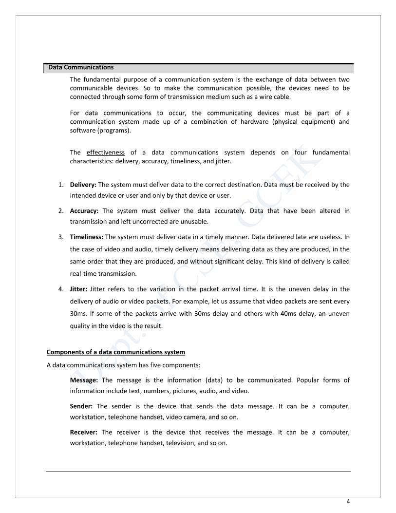
Protocol: A protocol is a set of rules that govern data communications. It represents an

agreement between the communicating devices. Without a protocol, two devices may be

connected but not communicating, just as a person speaking French cannot be understood by a

person who speaks only Japanese.

Fig. 1.1 components of data communication Data Flow Communication between two devices can be simplex, half-duplex, or full-duplex. Simplex

In simplex mode, the communication is unidirectional, as on a one-way street. Only one of the

two devices on a link can transmit; the other can only receive.

Keyboards and traditional monitors are examples of simplex devices. The keyboard can only

introduce input; the monitor can only accept output.

The simplex mode can use the entire capacity of the channel to send data in one direction.

Half-Duplex

In half-duplex mode, each station can both transmit and receive, but not at the same time.

When one device is sending, the other can only receive, and vice versa.

The half-duplex mode is like a one-lane road with traffic allowed in both directions. When cars

are traveling in one direction, cars going the other way must wait.

6

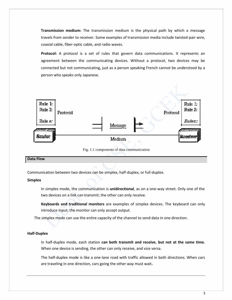
In a half-duplex transmission, the entire capacity of a channel is taken over by whichever of

the two devices is transmitting at the time.

Walkie-talkies and CB(citizens band) radios are both half-duplex systems.

Fig. 1.2 Data flow (simplex,half-duplex, and full-duplex)

Full Duplex

In full-duplex mode, both stations can transmit and receive simultaneously.

The full-duplex mode is like a two way street with traffic flowing in both directions at the

same time.

One common example of full-duplex communication is the telephone network. When two

people are communicating by a telephone line, both can talk and listen at the same time.

Network A network is a set of devices (often referred to as nodes) connected by communication links. A node can

be a computer, printer, or any other device capable of sending and/or receiving data generated by other

nodes on the network.

7

Distributed Processing Most networks use distributed processing, in which a task is divided among multiple computers. Instead

of one single large machine being responsible for all aspects of a process, separate computer (usually a

personal computer or workstation) handle a subset. Network Criteria A network must be able to meet a certain number of criteria. The most important of these are

performance, reliability, and security. Performance

Performance can be measured in many ways, including transmit time and response time.

Transmit time is the amount of time required for a message to travel from one device to

another. Response time is the elapsed time between an inquiry and a response.

The performance of a network depends on a number of factors, including the number of users,

the type of transmission medium, the capabilities of the connected hardware, and the efficiency

of the software.

Performance is often evaluated by two networking metrics: throughput and delay. We often

need more throughputs and less delay.

Reliability In addition to accuracy of delivery, network reliability is measured by the frequency of failure, the time it

takes a link to recover from a failure.

Security Network security issues include protecting data from unauthorized access, protecting data from damage

and development, and implementing policies and procedures for recovery from breaches and data losses.

Type of Connection

A network is two or more devices connected through links. A link is a communications pathway that

transfers data from one device to another. For visualization purposes, it is simplest to imagine any link

as a line drawn between two points.

Point-to-Point: A point-to-point connection provides a dedicated link between two devices. The entire

capacity of the link is reserved for transmission between those two devices.

Ex: changing television channels by infrared remote control.

8

Fig. 1.3 Types of connections: point-to-point and multipoint Multipoint: A multipoint (also called multi drop) connection is one in which more than two specific

devices share a single link. In a multipoint environment, the capacity of the channel is shared, either

spatially or temporally.

Physical Topology The term physical topology refers to the way in which a network is laid out physically: I/O or more

devices connect to a link; two or more links form a topology. There are four basic topologies possible: mesh, star, bus, and ring. Mesh Topology

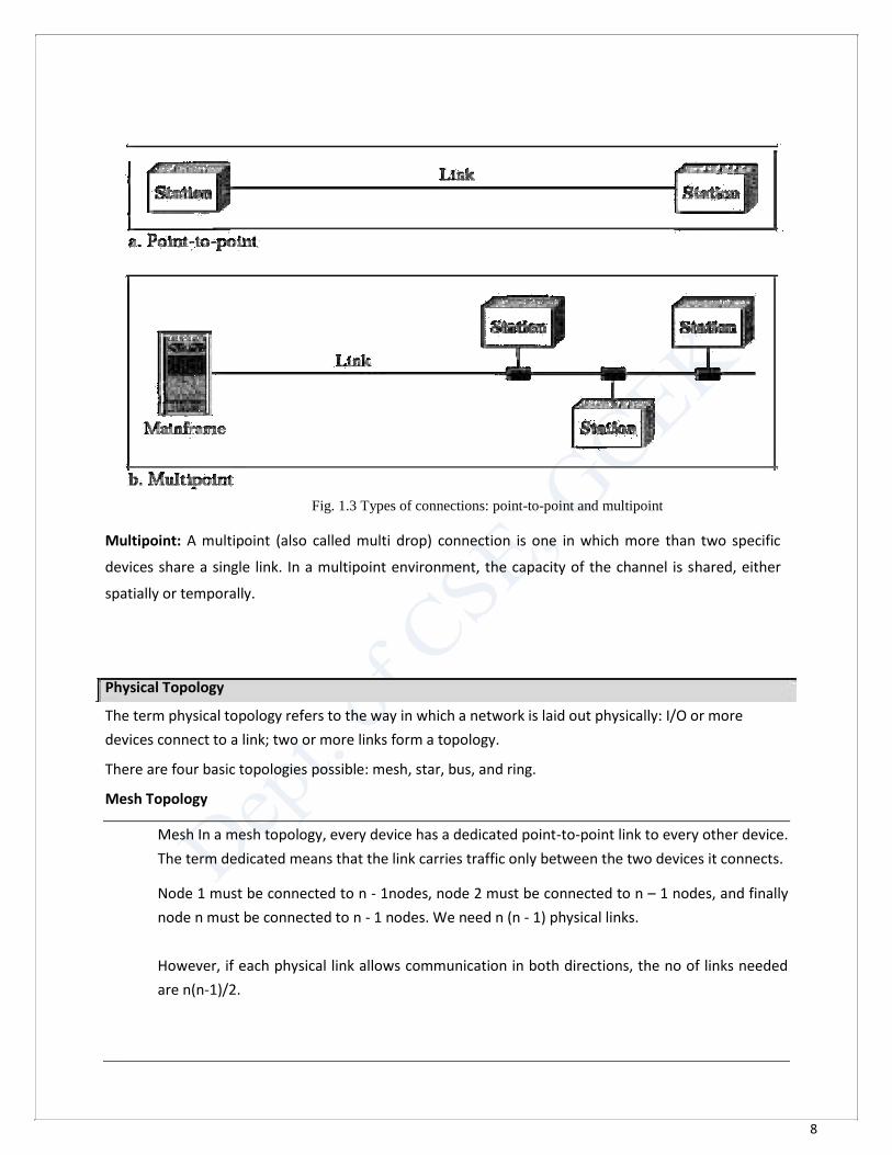
Mesh In a mesh topology, every device has a dedicated point-to-point link to every other device.

The term dedicated means that the link carries traffic only between the two devices it connects.

Node 1 must be connected to n - 1nodes, node 2 must be connected to n – 1 nodes, and finally

node n must be connected to n - 1 nodes. We need n (n - 1) physical links.

However, if each physical link allows communication in both directions, the no of links needed

are n(n-1)/2.

9

Fig. 1.4 star topology

Advantages

The use of dedicated links guarantees that each connection can carry its own data load, thus

eliminating the traffic problems that can occur when links must be shared by multiple devices.

A mesh topology is robust. If one link becomes unusable, it does not incapacitate the entire

system.

There is the advantage of privacy or security. When every message travels along a dedicated

line, only the intended recipient sees it.

Point-to-point links make fault identification and fault isolation easy.

Disadvantages

Amount of cabling and the number of I/O ports required.

The sheer bulk of the wiring can be greater than the available space (in walls, ceilings, or floors)

can accommodate.

The hardware required to connect each link (I/O ports and cable) can be prohibitively expensive.

Star Topology

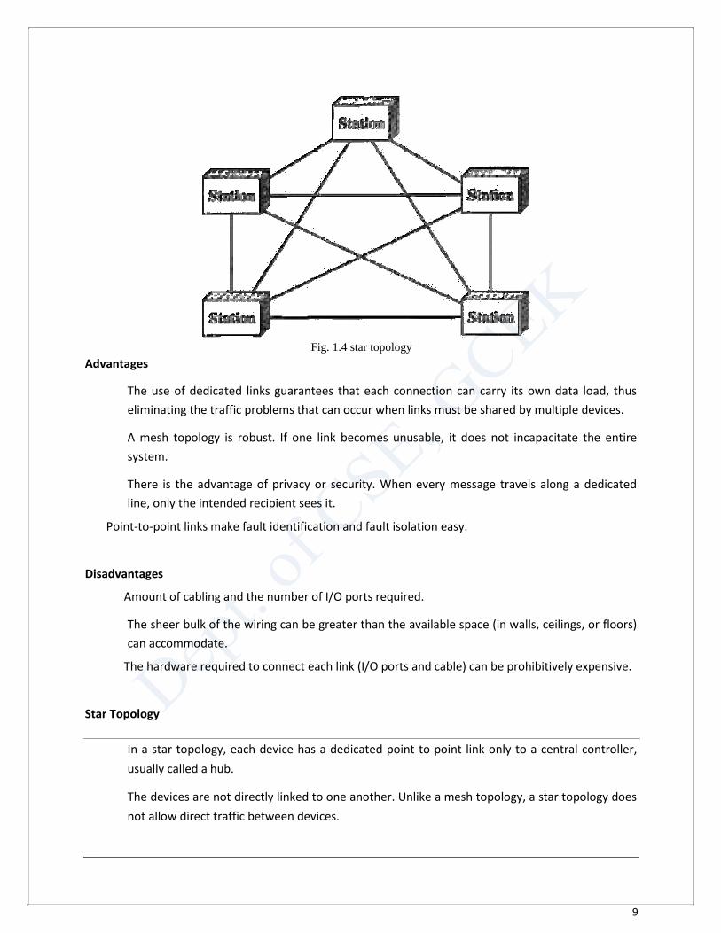
In a star topology, each device has a dedicated point-to-point link only to a central controller,

usually called a hub.

The devices are not directly linked to one another. Unlike a mesh topology, a star topology does

not allow direct traffic between devices.

10

The controller acts as an exchange: If one device wants to send data to another, it sends the data to

the controller, which then relays the data to the other connected device.

Fig. 1.5: star topology

Advantages

A star topology is less expensive than a mesh topology.

In a star, each device needs only one link and one I/O port to connect it to any number of

others. This factor also makes it easy to install and reconfigure.

Far less cabling needs to be housed, and additions, moves, and deletions involve only one

connection: between that device and the hub.

Other advantages include robustness. If one link fails, only that link is affected. All other links

remain active.

Disadvantages

The dependency of the whole topology bon one single point, the hub. If the hub goes down, the

whole system is dead.

Although a star requires far less cable than a mesh, each node must be linked to a central hub.

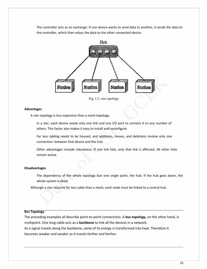
Bus Topology The preceding examples all describe point-to-point connections. A bus topology, on the other hand, is

multipoint. One long cable acts as a backbone to link all the devices in a network.

As a signal travels along the backbone, some of its energy is transformed into heat. Therefore it

becomes weaker and weaker as it travels farther and farther.

11

Fig. 1.6: bus topology

Advantages

Bus topology includes ease of installation.

A bus uses less cabling than mesh or star topologies.

Disadvantages

Difficult reconnection and fault isolation.

A fault or break in the bus cable stops all transmission, even between devices on the same side of

the problem.

Ring topology

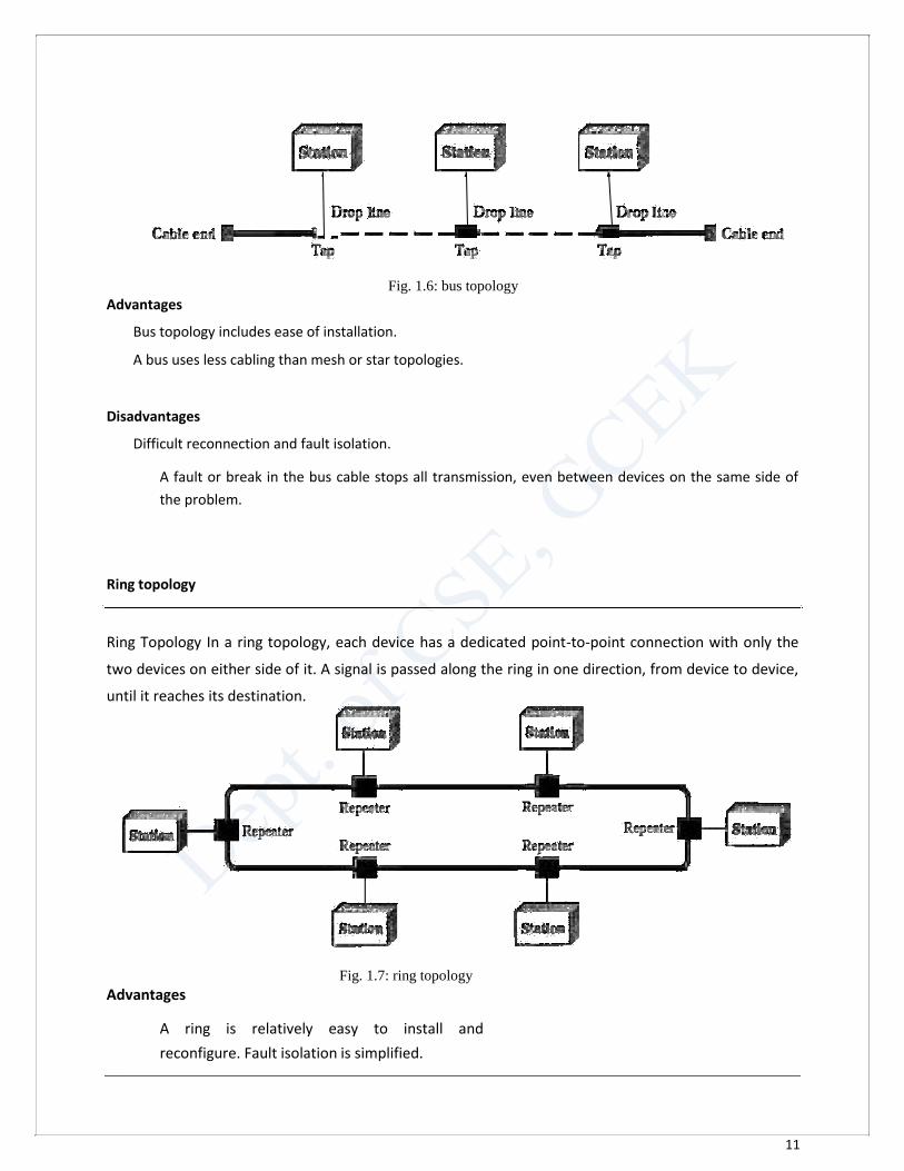
Ring Topology In a ring topology, each device has a dedicated point-to-point connection with only the

two devices on either side of it. A signal is passed along the ring in one direction, from device to device,

until it reaches its destination.

Fig. 1.7: ring topology Advantages

A ring is relatively easy to install and

reconfigure. Fault isolation is simplified.

12

Disadvantages

Unidirectional traffic can be a disadvantage.

In a simple ring, a break in the ring (such as a disabled station) can disable the entire network.

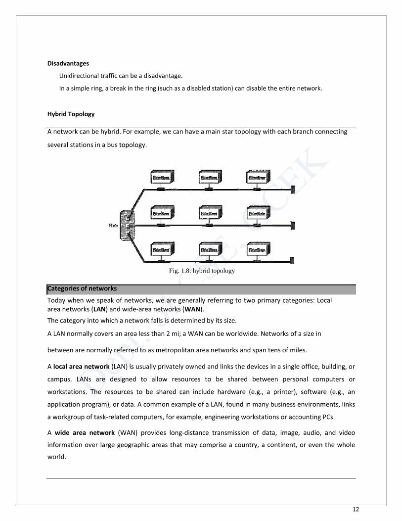
Hybrid Topology

A network can be hybrid. For example, we can have a main star topology with each branch connecting several stations in a bus topology. Fig. 1.8: hybrid topology Categories of networks Today when we speak of networks, we are generally referring to two primary categories: Local area networks (LAN) and wide-area networks (WAN). The category into which a network falls is determined by its size. A LAN normally covers an area less than 2 mi; a WAN can be worldwide. Networks of a size in between are normally referred to as metropolitan area networks and span tens of miles. A local area network (LAN) is usually privately owned and links the devices in a single office, building, or

campus. LANs are designed to allow resources to be shared between personal computers or

workstations. The resources to be shared can include hardware (e.g., a printer), software (e.g., an

application program), or data. A common example of a LAN, found in many business environments, links

a workgroup of task-related computers, for example, engineering workstations or accounting PCs. A wide area network (WAN) provides long-distance transmission of data, image, audio, and video

information over large geographic areas that may comprise a country, a continent, or even the whole

world.

13

A metropolitan area network (MAN) is a network with a size between a LAN and a WAN. It normally

covers the area inside a town or a city. It is designed for customers who need a high-speed connectivity,

normally to the Internet, and have endpoints spread over a city or part of city. A good example of a MAN

is the part of the telephone company network that can provide a high-speed DSL line to the customer.

Most common LAN topologies are bus, ring and star.

Distance Location Network Used 10 meters Classroom LAN 100 meters Building LAN 1000 meters Campus LAN 2-50 kilometers City MAN 100 kilometers County WAN 1,000 kilometers Continent WAN 10,000 kilometers Planet – Internet WAN

14

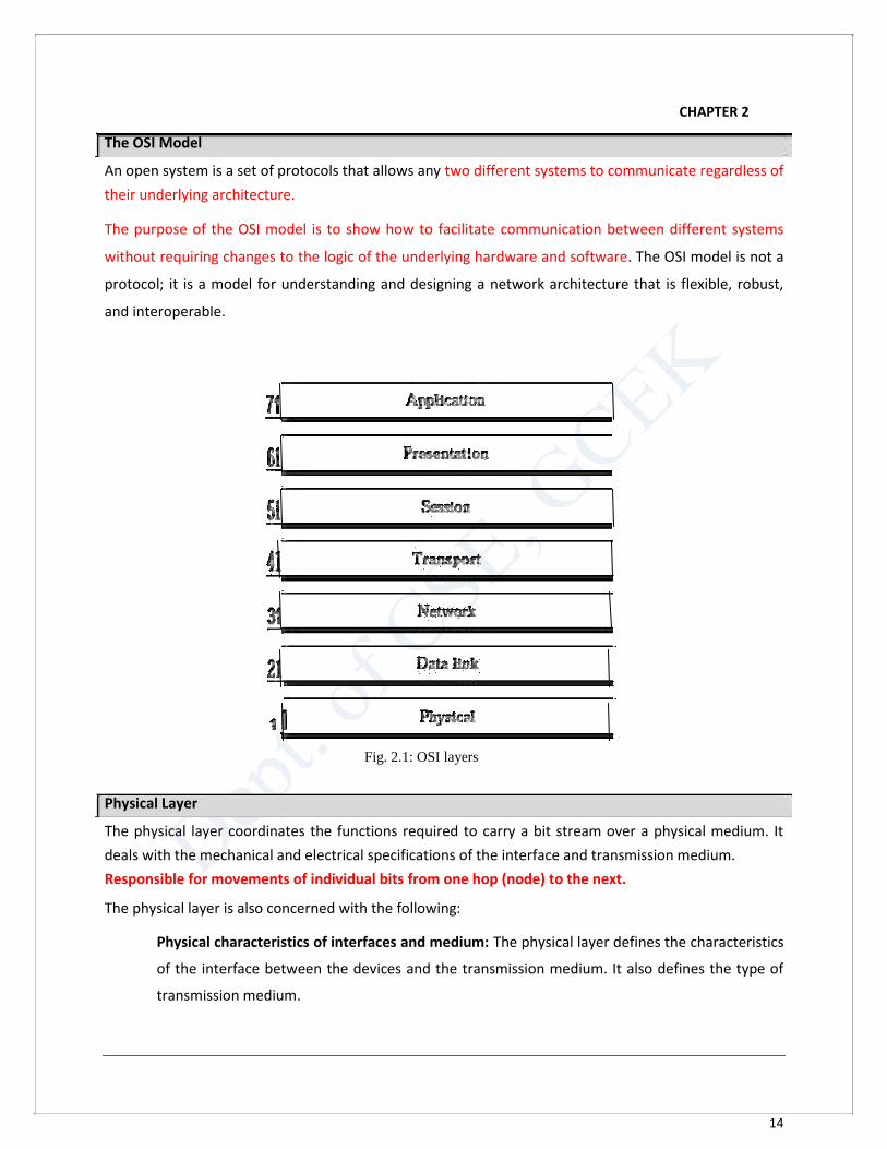
CHAPTER 2 The OSI Model An open system is a set of protocols that allows any two different systems to communicate regardless of

their underlying architecture. The purpose of the OSI model is to show how to facilitate communication between different systems

without requiring changes to the logic of the underlying hardware and software. The OSI model is not a

protocol; it is a model for understanding and designing a network architecture that is flexible, robust,

and interoperable.

Fig. 2.1: OSI layers

Physical Layer The physical layer coordinates the functions required to carry a bit stream over a physical medium. It

deals with the mechanical and electrical specifications of the interface and transmission medium.

Responsible for movements of individual bits from one hop (node) to the next. The physical layer is also concerned with the following:

Physical characteristics of interfaces and medium: The physical layer defines the characteristics

of the interface between the devices and the transmission medium. It also defines the type of

transmission medium.

15

Representation of bits: The physical layer data consists of a stream of bits (sequence of Os or 1s)

with no interpretation. To be transmitted, bits must be encoded into signals--electrical or optical.

The physical layer defines the type of encoding (how Os and I s are changed to signals).

Data rate: The transmission rate-the number of bits sent each second-is also defined by the physical

layer. In other words, the physical layer defines the duration of a bit, which is how long it lasts.

Synchronization of bits: The sender and receiver not only must use the same bit rate but also must

be synchronized at the bit level. In other words, the sender and the receiver clocks must be

synchronized.

Line configuration: The physical layer is concerned with the connection of devices to the media. In a

point-to-point configuration, two devices are connected through a dedicated link. In a multipoint

configuration, a link is shared among several devices.

Physical topology: The physical topology defines how devices are connected to make a network.

Devices can be connected by using a mesh topology (every device is connected to every other

device), a star topology (devices are connected through a central device), a ring topology (each

device is connected to the next, forming a ring), a bus topology (every device is on a common link),

or a hybrid topology (this is a combination of two or more topologies).

Transmission mode: The physical layer also defines the direction of transmission between two

devices: simplex, half-duplex, or full-duplex. In simplex mode, only one device can send; the other

can only receive. The simplex mode is a one-way communication. In the half-duplex mode, two

devices can send and receive, but not at the same time. In a full-duplex (or simply duplex) mode, two

devices can send and receive at the same time.

Data Link Layer The data link layer transforms the physical layer, a raw transmission facility, to a reliable link. It makes

the physical layer appear error-free to the upper layer (network layer).

Responsible for moving frames from one hop (node) to the next. Other responsibilities of the data link layer include the following:

Framing: The data link layer divides the stream of bits received from the network layer into

manageable data units called frames.

Physical addressing: If frames are to be distributed to different systems on the network, the

data link layer adds a header to the frame to define the sender and/or receiver of the frame. If

16

the frame is intended for a system outside the sender's network, the receiver address is the address

of the device that connects the network to the next one.

Flow control: If the rate at which the data are absorbed by the receiver is less than the rate at which

data are produced in the sender, the data link layer imposes a flow control mechanism to avoid

overwhelming the receiver.

Error control: The data link layer adds reliability to the physical layer by adding mechanisms to

detect and retransmit damaged or lost frames. It also uses a mechanism to recognize duplicate

frames. Error control is normally achieved through a trailer added to the end of the frame.

Access control: When two or more devices are connected to the same link, data link layer protocols

are necessary to determine which device has control over the link at any given time.

Network Layer The network layer is responsible for the source-to-destination delivery of a packet, possibly across

multiple networks (links). Whereas the data link layer oversees the delivery of the packet between two

systems on the same network (links), the network layer ensures that each packet gets from its point of

origin to its final destination. Other responsibilities of the network layer include the following:

Logical addressing. The physical addressing implemented by the data link layer handles the

addressing problem locally. If a packet passes the network boundary, we need another

addressing system to help distinguish the source and destination systems. The network layer

adds a header to the packet coming from the upper layer that, among other things, includes the

logical addresses of the sender and receiver. We discuss logical addresses later in this chapter.

Routing. When independent networks or links are connected to create internetworks (network

of networks) or a large network, the connecting devices (called routers or switches) route or

switch the packets to their final destination. One of the functions of the network layer is to

provide this mechanism. Transport Layer The transport layer is responsible for process-to-process delivery of the entire message. A process is an

application program running on a host. Whereas the network layer oversees source-to-destination

delivery of individual packets, it does not recognize any relationship between those packets. Other responsibilities of the transport layer include the following:

17

Service-point addressing: Computers often run several programs at the same time. For this reason,

source-to-destination delivery means delivery not only from one computer to the next but also from

a specific process (running program) on one computer to a specific process (running program) on the

other. The transport layer header must therefore include a type of address called a service-point

address (or port address). The network layer gets each packet to the correct computer; the transport

layer gets the entire message to the correct process on that computer.

Segmentation and reassembly: A message is divided into transmittable segments, with each

segment containing a sequence number. These numbers enable the transport layer to reassemble

the message correctly upon arriving at the destination and to identify and replace packets that were

lost in transmission.

Connection control: The transport layer can be either connectionless or connection oriented.

A connectionless transport layer treats each segment as an independent packet and delivers it to the

transport layer at the destination machine. A connection oriented transport layer makes a

connection with the transport layer at the destination machine first before delivering the packets.

After all the data are transferred, the connection is terminated.

Flow control: Like the data link layer, the transport layer is responsible for flow control. However,

flow control at this layer is performed end to end rather than across a single link.

Error control: Like the data link layer, the transport layer is responsible for error control. However,

error control at this layer is performed process-to process rather than across a single link. The

sending transport layer makes sure that the entire message arrives at the receiving transport layer

without error (damage, loss, or duplication). Error correction is usually achieved through

retransmission.

Session Layer The services provided by the first three layers (physical, data link, and network) are not sufficient for

some processes. The session layer is the network dialog controller. It establishes, maintains, and

synchronizes the interaction among communicating systems. The session layer is responsible for dialog

control and synchronization.

Also used to establish, manage and terminate sessions.

18

Specific responsibilities of the session layer include the following: Dialog control: The session layer allows two systems to enter into a dialog. It allows the communication between two processes to take place in either half duplex (one way at a time) or full-duplex (two ways at a time) mode. Synchronization: The session layer allows a process to add checkpoints, or synchronization points, to a stream of

data. For example, if a system is sending a file of 2000 pages, it is advisable to insert checkpoints after every 100

pages to ensure that each 100-page unit is received and acknowledged independently. In this case, if a crash

happens during the transmission of page 523, the only pages that need to be resent after system recovery are

pages 501 to 523. Pages previous to 501 need not be resent.

Presentation Layer The presentation layer is concerned with the syntax and semantics of the information exchanged between two systems. Specific responsibilities of the presentation layer include the following:

Translation: The processes (running programs) in two systems are usually exchanging

information in the form of character strings, numbers, and so on. The information must be

changed to bit streams before being transmitted. Because different computers use different

encoding systems, the presentation layer is responsible for interoperability between these

different encoding methods. The presentation layer at the sender changes the information from

its sender-dependent format into a common format. The presentation layer at the receiving

machine changes the common format into its receiver-dependent format.

Encryption: To carry sensitive information, a system must be able to ensure privacy. Encryption

means that the sender transforms the original information another form and sends the resulting

message out over the network. Decryption reverses the original process to transform the

message back to its original form.

Compression: Data compression reduces the number of bits contained in the information. Data

compression becomes particularly important in the transmission of multimedia such as text,

audio, and video.

19

Application Layer The application layer enables the user, whether human or software, to access the network. It provides

user interfaces and support for services such as electronic mail, remote file access and transfer, shared

database management, and other types of distributed information services, ex. FTAM used for file

transfer and management, X.400 for message handling and X.500 for directory services.

TCP/IP Protocol Suites:

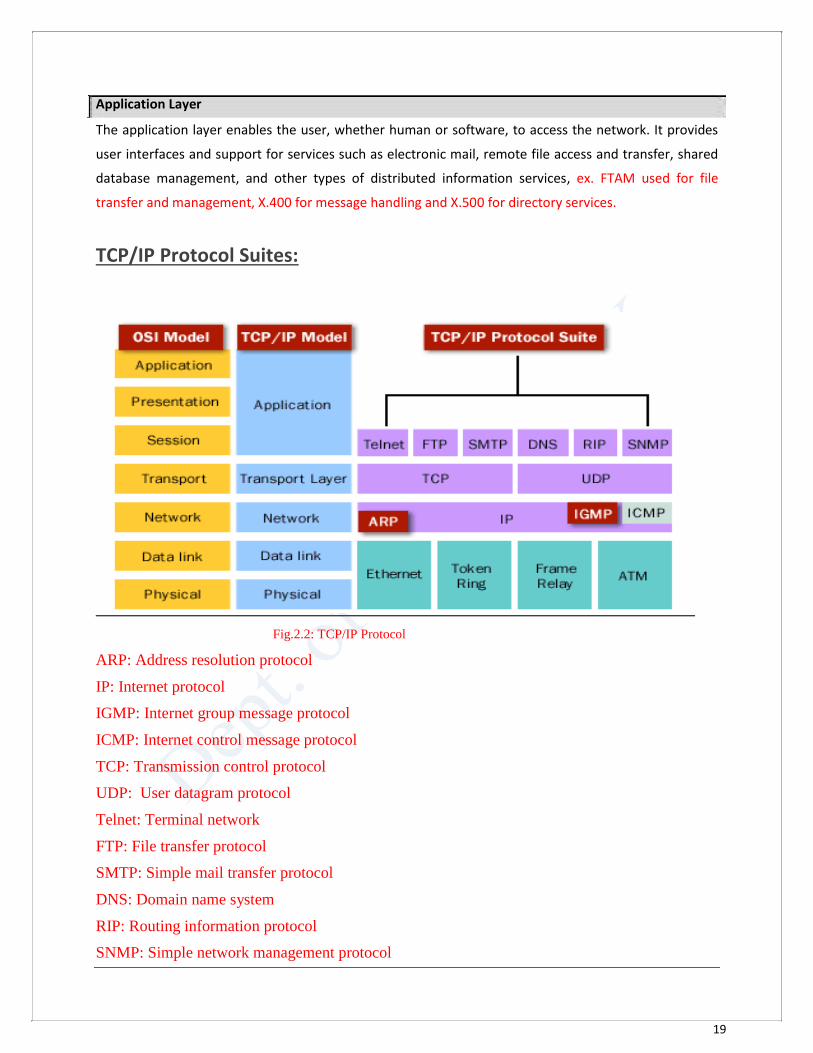
Fig.2.2: TCP/IP Protocol ARP: Address resolution protocol IP: Internet protocol IGMP: Internet group message protocol ICMP: Internet control message protocol TCP: Transmission control protocol UDP: User datagram protocol Telnet: Terminal network FTP: File transfer protocol SMTP: Simple mail transfer protocol DNS: Domain name system RIP: Routing information protocol SNMP: Simple network management protocol

20

CHAPTER 3 ANALOG AND DIGITAL SIGNAL

One of the major functions of the physical layer is to move data in the form of electromagnetic

signals across a transmission medium.

Both data and the signals that represent them can be either analog or digital in form.

Analog and Digital Data

Data can be analog or digital. The term analog data refers to information that is continuous;

digital data refers to information that has discrete states.

For example, an analog clock that has hour, minute, and second hands gives information in a

continuous form; the movements of the hands are continuous. On the other hand, a digital clock

that reports the hours and the minutes will change suddenly from 8:05 to 8:06.

Analog data, such as the sounds made by a human voice, take on continuous values. When

someone speaks, an analog wave is created in the air. This can be captured by a microphone and

converted to an analog signal or sampled and converted to a digital signal.

Digital data take on discrete values. For example, data are stored in computer memory in the

form of Os and 1s. They can be converted to a digital signal or modulated into an analog signal

for transmission across a medium.

Analog and Digital Signals

Like the data they represent, signals can be either analog or digital. An analog signal has

infinitely many levels of intensity over a period of time.

A digital signal, on the other hand, can have only a limited number of defined values. Although

each value can be any number, it is often as simple as 1 and 0.

Periodic and Non periodic Signals

Both analog and digital signals can take one of two forms: periodic or non periodic.

A periodic signal completes a pattern within a measurable time frame, called a period, and

repeats that pattern over subsequent identical periods. The completion of one full pattern is

called a cycle.

A non periodic signal changes without exhibiting a pattern or cycle that repeats over time.

21

Both analog and digital signals can be periodic or non periodic. In data communications, we

commonly use periodic analog signals (because they need less bandwidth) and non periodic digital

signals (because they can represent variation in data).

Periodic Analog Signals

Periodic analog signals can be classified as simple or composite.

A simple periodic analog signal, a sine wave, cannot be decomposed into simpler signals.

A composite periodic analog signal is composed of multiple sine waves.

Sine Wave

The sine wave is the most fundamental form of a periodic analog signal. When we visualize it as

a simple oscillating curve, its change over the course of a cycle is smooth and consistent, a

continuous, rolling flow.

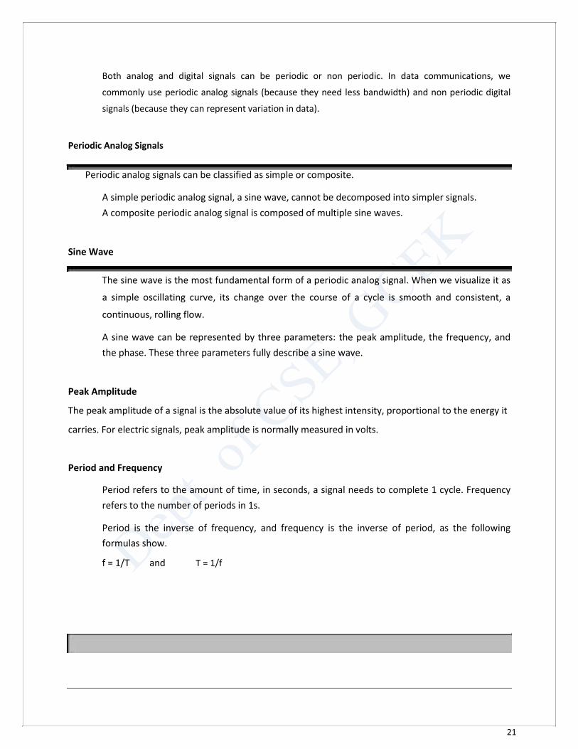
A sine wave can be represented by three parameters: the peak amplitude, the frequency, and

the phase. These three parameters fully describe a sine wave.

Peak Amplitude The peak amplitude of a signal is the absolute value of its highest intensity, proportional to the energy it carries. For electric signals, peak amplitude is normally measured in volts.

Period and Frequency

Period refers to the amount of time, in seconds, a signal needs to complete 1 cycle. Frequency

refers to the number of periods in 1s.

Period is the inverse of frequency, and frequency is the inverse of period, as the following

formulas show.

f = 1/T and T = 1/f

22

Milliseconds (ms) 10-3

s Kilohertz (kHz)

Microseconds (µs) 10-6

s Megahertz (MHz

Nanoseconds (ns) 10-9

s Gigahertz (GHz)

Picoseconds (ps) 10-12 s Terahertz (THz)

Fig. 2.3: signal with different amplitudes Composite Signals

Simple sine waves have many applications in daily life. We can send a single sine wave to carry

electric energy from one place to another. For example, the power company sends a single sine

wave with a frequency of 60 Hz to distribute electric energy to houses and businesses.

A single frequency sine wave is not useful in data communications; we need to send a

composite signal, a signal made of many simple sine waves.

According to Fourier analysis, any composite signal is a combination of simple sine waves with

different frequencies, amplitudes, and phases.

Unit Equivalent Unit

Seconds (s) 1 s Hertz (Hz)

23

Bandwidth

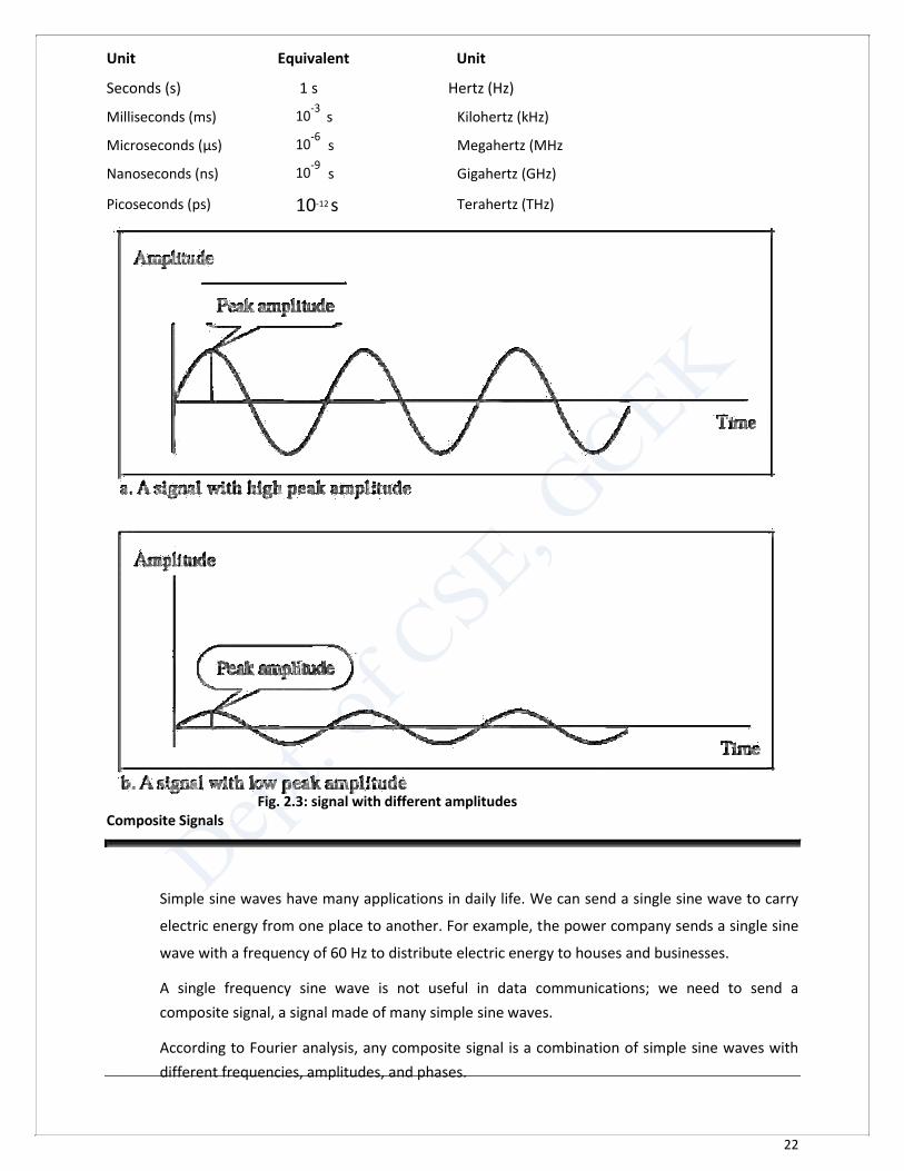
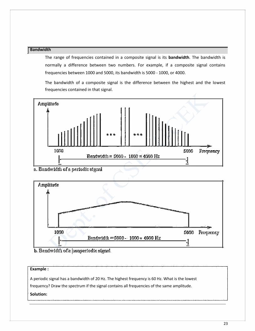
The range of frequencies contained in a composite signal is its bandwidth. The bandwidth is

normally a difference between two numbers. For example, if a composite signal contains

frequencies between 1000 and 5000, its bandwidth is 5000 - 1000, or 4000.

The bandwidth of a composite signal is the difference between the highest and the lowest

frequencies contained in that signal.

Example : A periodic signal has a bandwidth of 20 Hz. The highest frequency is 60 Hz. What is the lowest

frequency? Draw the spectrum if the signal contains all frequencies of the same amplitude. Solution:

24

Let fh be the highest frequency, fz the lowest frequency, and B the bandwidth.

Then B =fh - fz 20 =60 - fz or fz =60 - 20=40 Hz

Digital Signal In addition to being represented by an analog signal, information can also be represented by a digital

signal. For example, 1 can be encoded as a positive voltage and a 0 as zero voltage. A digital signal can

have more than two levels.

In general, if a signal has L levels, each level needs log2 L bits. Example: A digital signal has eight levels. How many bits are needed per level? Solution: We calculate the number of bits from the formula: Number of bits per level =log2 8 =3 Each signal level is represented by 3 bits.

Bit Rate

Most digital signals are non periodic, and thus period and frequency are not appropriate

characteristics. Another term-bit rate is used to describe digital signals.

The bit rate is the number of bits sent in 1s, expressed in bits per second (bps). Example : Assume we need to download text documents at the rate of 100 pages per minute. What is the required

bit rate of the channel? Solution: A page is an average of 24 lines with 80 characters in each line. If we assume that one character requires

8 bits, the bit rate is 100 x 24 x 80 x 8 =1,636,000 bps =1.636 Mbps Bit Length We discussed the concept of the wavelength for an analog signal: the distance one cycle occupies on the

transmission medium. We can define something similar for a digital signal: the bit length. The bit length

is the distance one bit occupies on the transmission medium. Bit length=propagation speed x bit duration

25

Data Rate Limits A very important consideration in data communications is how fast we can send data, in bits per second

over a channel. Data rate depends on three factors: 1. The bandwidth available 2. The level of the signals we use 3. The quality of the channel (the level of noise) Two theoretical formulas were developed to calculate the data rate: one by Nyquist for a noiseless

channel, another by Shannon for a noisy channel.

Noiseless Channel: Nyquist Bit Rate For a noiseless channel, the Nyquist bit rate formula defines the theoretical maximum bit rate BitRate = 2 x bandwidth x l0g2 L In this formula, bandwidth is the bandwidth of the channel, L is the number of signal levels used to

represent data, and Bit Rate is the bit rate in bits per second. Example: Consider a noiseless channel with a bandwidth of 3000 Hz transmitting a signal with two signal levels.

The maximum bit rate can be calculated as BitRate =2 x 3000 x log2 2 =6000 bps

Noisy Channel: Shannon Capacity In reality, we cannot have a noiseless channel; the channel is always noisy. In 1944, Claude Shannon

introduced a formula, called the Shannon capacity, to determine the theoretical highest data rate for a

noisy channel:

Capacity =bandwidth X log2 (1 +SNR) In this formula, bandwidth is the bandwidth of the channel, SNR is the signal-to-noise ratio, and capacity

is the capacity of the channel in bits per second. Note that in the Shannon formula there is no indication

of the signal level, which means that no matter how many levels we have, we cannot achieve a data rate

higher than the capacity of the channel. In other words, the formula defines a characteristic of the

channel, not the method of transmission.

26

Example: Consider an extremely noisy channel in which the value of the signal-to-noise ratio is almost zero. In

other words, the noise is so strong that the signal is faint. For this channel the capacity C is calculated as

C=B log2 (1 + SNR) =B l0g2 (1 + 0) =B log2 1 = B x 0 =0 This means that the capacity of this channel is zero regardless of the bandwidth. In other words, we

cannot receive any data through this channel.

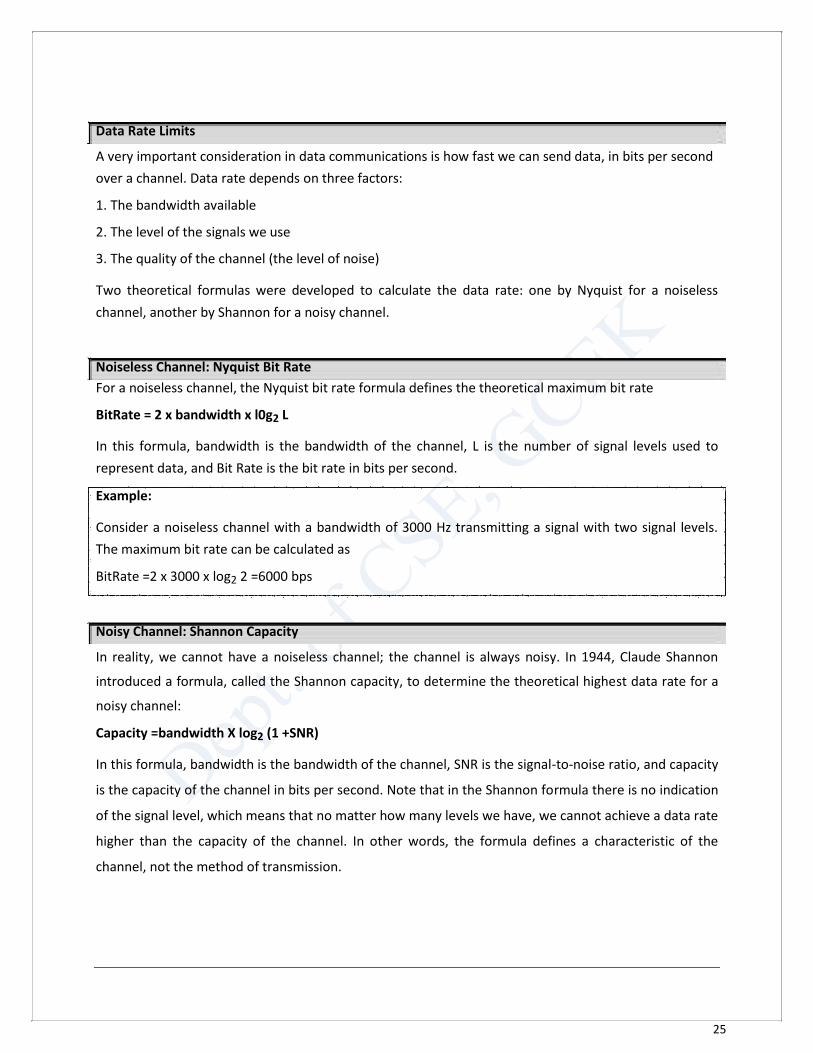
Transmission Impairment Signals travel through transmission media, which are not perfect. The imperfection causes signal

impairment. This means that the signal at the beginning of the medium is not the same as the signal at

the end of the medium. What is sent is not what is received. Three causes of impairment are

attenuation, distortion, and noise.

Attenuation Attenuation means a loss of energy. When a signal, simple or composite, travels through a medium, it

loses some of its energy in overcoming the resistance of the medium. That is why a wire carrying electric

signals gets warm, if not hot, after a while. Some of the electrical energy in the signal is converted to

heat. To compensate for this loss, amplifiers are used to amplify the signal.

Decibel

To show that a signal has lost or gained strength, engineers use the unit of the decibel.

The decibel (dB) measures the relative strengths of two signals or one signal at two different

points.

Note that the decibel is negative if a signal is attenuated and positive if a signal is amplified.

27

Variables PI and P2 are the powers of a signal at points 1 and 2, respectively. Example: Suppose a signal travels through a transmission medium and its power is reduced to one-half. Find

the attenuation (loss of power). Solution: dB=10 log (P/2P)= -3 dB

Example: A signal travels through an amplifier, and its power is increased 10 times Find the amplification (gain of

power). Solution: dB=10 log (10P/P)= 10 dB

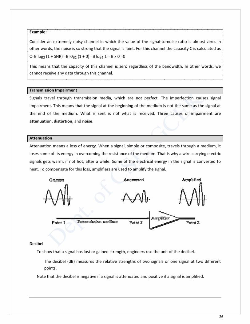
Distortion Distortion means that the signal changes its form or shape.

Distortion can occur in a composite signal made of different frequencies. Each signal component

has its own propagation speed (see the next section) through a medium and, therefore, its own

delay in arriving at the final destination. Differences in delay may create a difference in phase if

the delay is not exactly the same as the period duration.

In other words, signal components at the receiver have phases different from what they had at

the sender. The shape of the composite signal is therefore not the same.

28

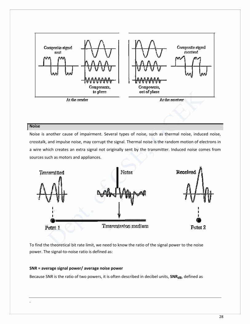
Noise Noise is another cause of impairment. Several types of noise, such as thermal noise, induced noise,

crosstalk, and impulse noise, may corrupt the signal. Thermal noise is the random motion of electrons in

a wire which creates an extra signal not originally sent by the transmitter. Induced noise comes from

sources such as motors and appliances.

To find the theoretical bit rate limit, we need to know the ratio of the signal power to the noise

power. The signal-to-noise ratio is defined as:

SNR = average signal power/ average noise power Because SNR is the ratio of two powers, it is often described in decibel units, SNRdB, defined as

.

29

Example The power of a signal is 10 mW and the power of the noise is 1 µW; what are the values of SNR

and SNRdB? Solution: The values of SNR and SNRdB can be calculated as follows: SNR = 10

-2/10

-6 =10, 000

SNRdB =10 log 1010

4 =10 × 4=40

Performance: The performance can be by checking the following parameters.

1) Bandwidth: can be represented in terms of hertz as well as bits per second. The bandwidth utilization should be high.

2) Throughput: is a measure of how fast we can actually send data through a network. So we may have a link with a bandwidth of 1 mbps, but we can only send let 300 kbps. So the throughput is 300kbps. The throughput should be high.

3) Latency: it defines how long it takes for an entire message to completely arrive at the destination from the time the 1st bit is sent out from the source. Latency= propagation time + transmission time + queuing time + processing time

The latency should be low.

30

This page is left vacant intentionally

31

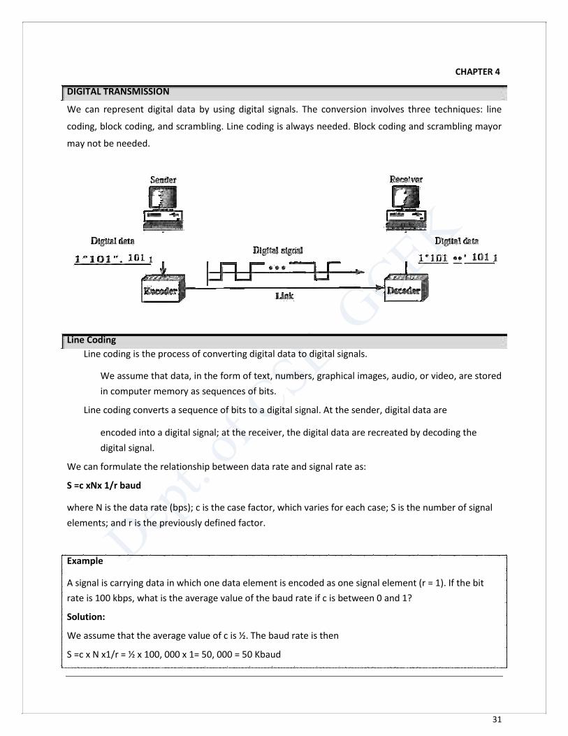
CHAPTER 4 DIGITAL TRANSMISSION We can represent digital data by using digital signals. The conversion involves three techniques: line

coding, block coding, and scrambling. Line coding is always needed. Block coding and scrambling mayor

may not be needed.

Line Coding

Line coding is the process of converting digital data to digital signals.

We assume that data, in the form of text, numbers, graphical images, audio, or video, are stored

in computer memory as sequences of bits.

Line coding converts a sequence of bits to a digital signal. At the sender, digital data are

encoded into a digital signal; at the receiver, the digital data are recreated by decoding the

digital signal. We can formulate the relationship between data rate and signal rate as: S =c xNx 1/r baud where N is the data rate (bps); c is the case factor, which varies for each case; S is the number of signal

elements; and r is the previously defined factor.

Example A signal is carrying data in which one data element is encoded as one signal element (r = 1). If the bit

rate is 100 kbps, what is the average value of the baud rate if c is between 0 and 1? Solution: We assume that the average value of c is ½. The baud rate is then S =c x N x1/r = ½ x 100, 000 x 1= 50, 000 = 50 Kbaud

32

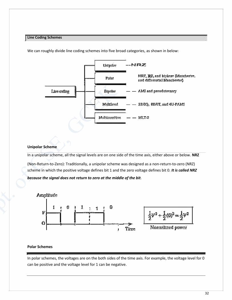
Line Coding Schemes We can roughly divide line coding schemes into five broad categories, as shown in below: Unipolar Scheme In a unipolar scheme, all the signal levels are on one side of the time axis, either above or below. NRZ (Non-Return-to-Zero): Traditionally, a unipolar scheme was designed as a non-return-to-zero (NRZ)

scheme in which the positive voltage defines bit 1 and the zero voltage defines bit 0. It is called NRZ because the signal does not return to zero at the middle of the bit.

Polar Schemes

In polar schemes, the voltages are on the both sides of the time axis. For example, the voltage level for 0

can be positive and the voltage level for 1 can be negative.

33

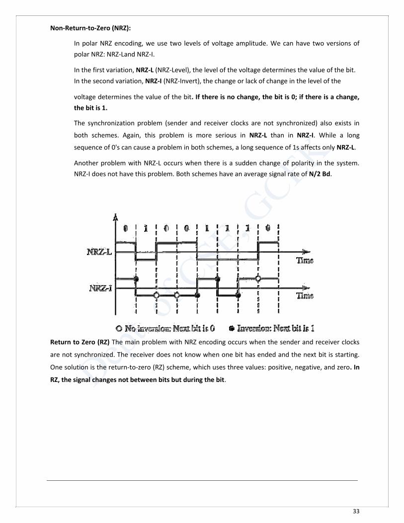
Non-Return-to-Zero (NRZ):

In polar NRZ encoding, we use two levels of voltage amplitude. We can have two versions of

polar NRZ: NRZ-Land NRZ-I.

In the first variation, NRZ-L (NRZ-Level), the level of the voltage determines the value of the bit.

In the second variation, NRZ-I (NRZ-Invert), the change or lack of change in the level of the

voltage determines the value of the bit. If there is no change, the bit is 0; if there is a change,

the bit is 1.

The synchronization problem (sender and receiver clocks are not synchronized) also exists in

both schemes. Again, this problem is more serious in NRZ-L than in NRZ-I. While a long

sequence of 0's can cause a problem in both schemes, a long sequence of 1s affects only NRZ-L.

Another problem with NRZ-L occurs when there is a sudden change of polarity in the system.

NRZ-I does not have this problem. Both schemes have an average signal rate of N/2 Bd.

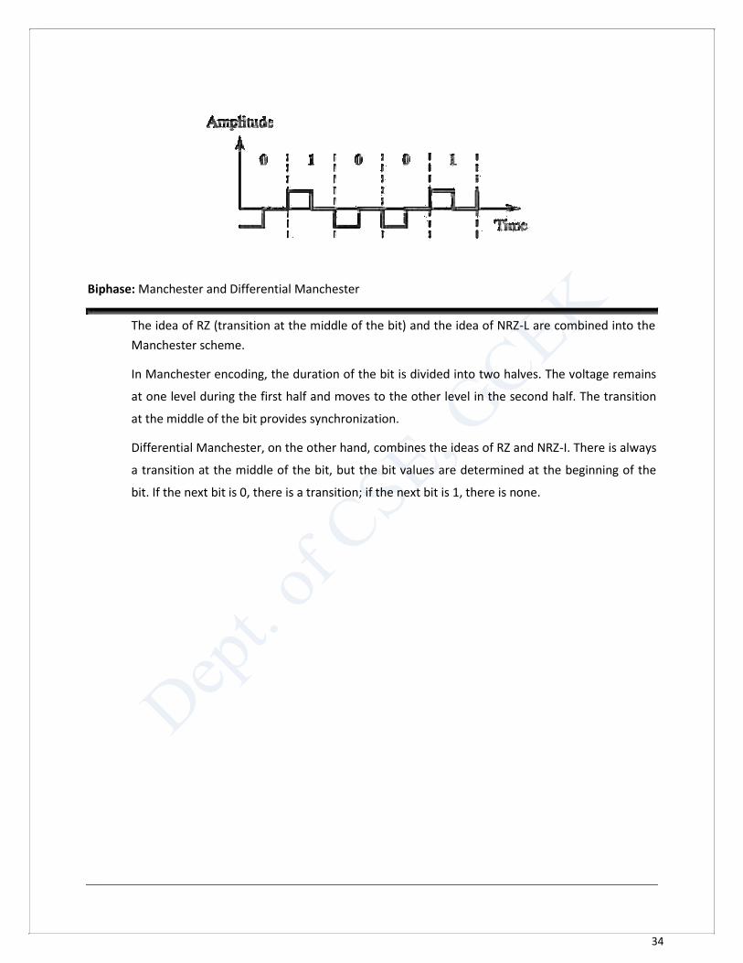
Return to Zero (RZ) The main problem with NRZ encoding occurs when the sender and receiver clocks

are not synchronized. The receiver does not know when one bit has ended and the next bit is starting.

One solution is the return-to-zero (RZ) scheme, which uses three values: positive, negative, and zero. In

RZ, the signal changes not between bits but during the bit.

34

Biphase: Manchester and Differential Manchester

The idea of RZ (transition at the middle of the bit) and the idea of NRZ-L are combined into the

Manchester scheme.

In Manchester encoding, the duration of the bit is divided into two halves. The voltage remains

at one level during the first half and moves to the other level in the second half. The transition

at the middle of the bit provides synchronization.

Differential Manchester, on the other hand, combines the ideas of RZ and NRZ-I. There is always

a transition at the middle of the bit, but the bit values are determined at the beginning of the

bit. If the next bit is 0, there is a transition; if the next bit is 1, there is none.

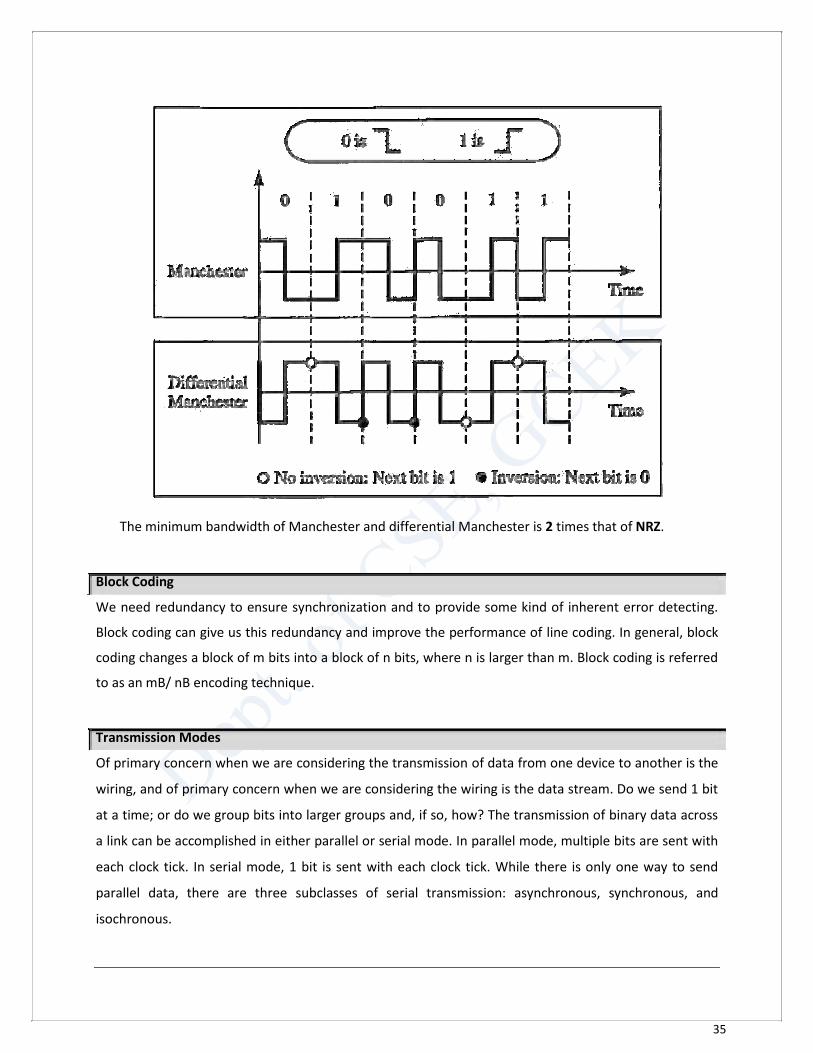
35

The minimum bandwidth of Manchester and differential Manchester is 2 times that of NRZ.

Block Coding We need redundancy to ensure synchronization and to provide some kind of inherent error detecting.

Block coding can give us this redundancy and improve the performance of line coding. In general, block

coding changes a block of m bits into a block of n bits, where n is larger than m. Block coding is referred

to as an mB/ nB encoding technique.

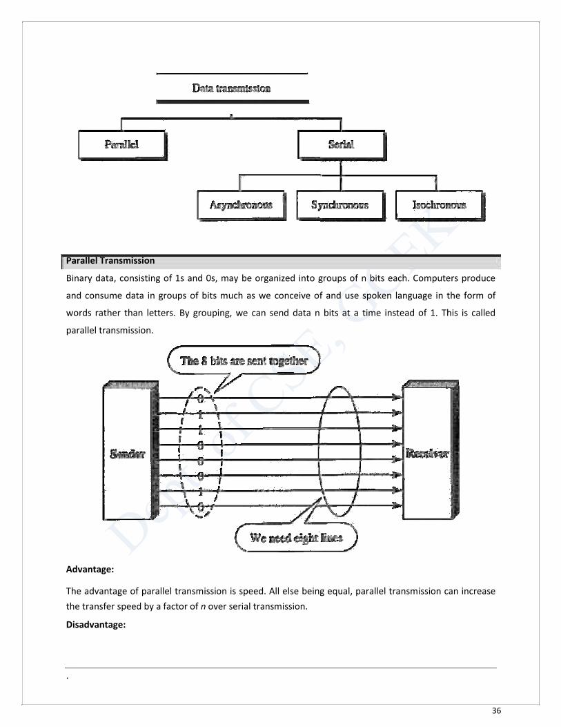
Transmission Modes Of primary concern when we are considering the transmission of data from one device to another is the

wiring, and of primary concern when we are considering the wiring is the data stream. Do we send 1 bit

at a time; or do we group bits into larger groups and, if so, how? The transmission of binary data across

a link can be accomplished in either parallel or serial mode. In parallel mode, multiple bits are sent with

each clock tick. In serial mode, 1 bit is sent with each clock tick. While there is only one way to send

parallel data, there are three subclasses of serial transmission: asynchronous, synchronous, and

isochronous.

36

Parallel Transmission Binary data, consisting of 1s and 0s, may be organized into groups of n bits each. Computers produce

and consume data in groups of bits much as we conceive of and use spoken language in the form of

words rather than letters. By grouping, we can send data n bits at a time instead of 1. This is called

parallel transmission.

Advantage: The advantage of parallel transmission is speed. All else being equal, parallel transmission can increase

the transfer speed by a factor of n over serial transmission. Disadvantage: .

37

Parallel transmission requires n communication lines just to transmit the data stream. Because this is expensive, parallel transmission is usually limited to short distances.

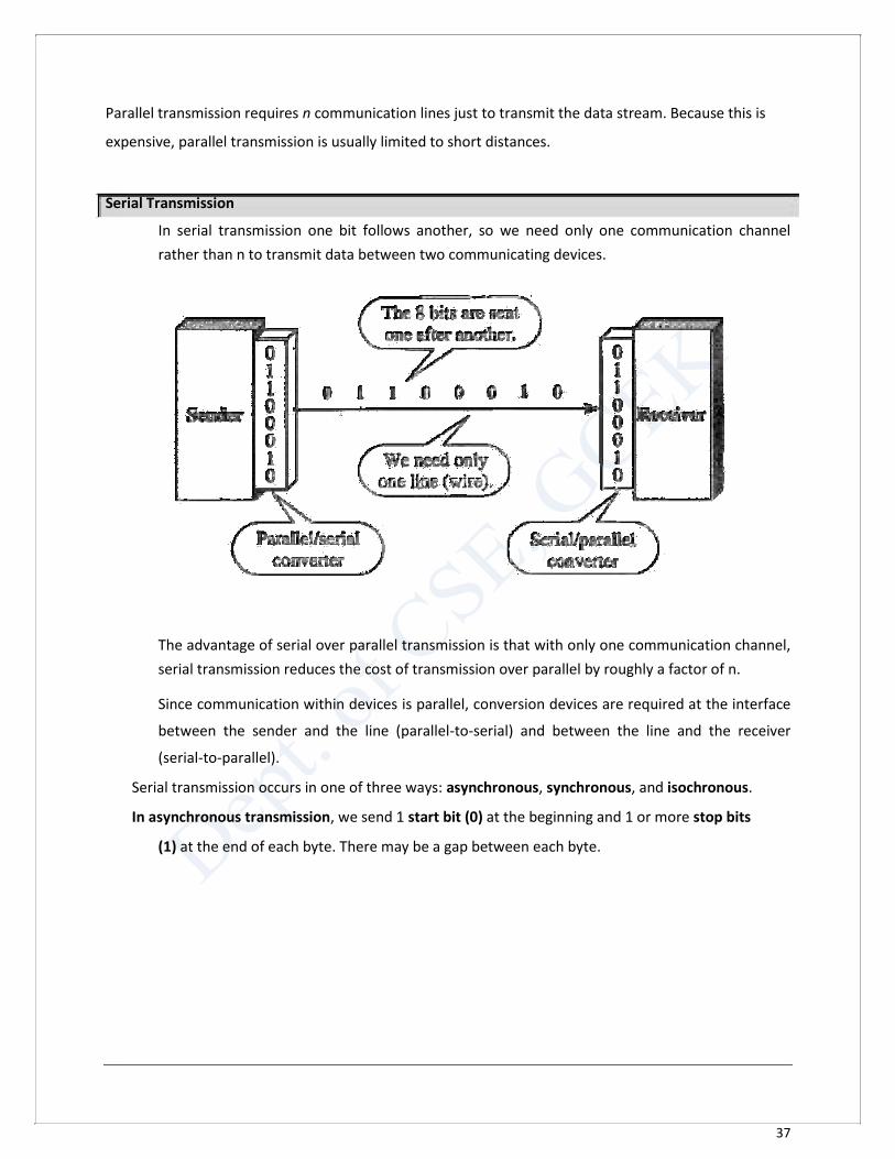
Serial Transmission

In serial transmission one bit follows another, so we need only one communication channel

rather than n to transmit data between two communicating devices.

The advantage of serial over parallel transmission is that with only one communication channel,

serial transmission reduces the cost of transmission over parallel by roughly a factor of n.

Since communication within devices is parallel, conversion devices are required at the interface

between the sender and the line (parallel-to-serial) and between the line and the receiver

(serial-to-parallel).

Serial transmission occurs in one of three ways: asynchronous, synchronous, and isochronous.

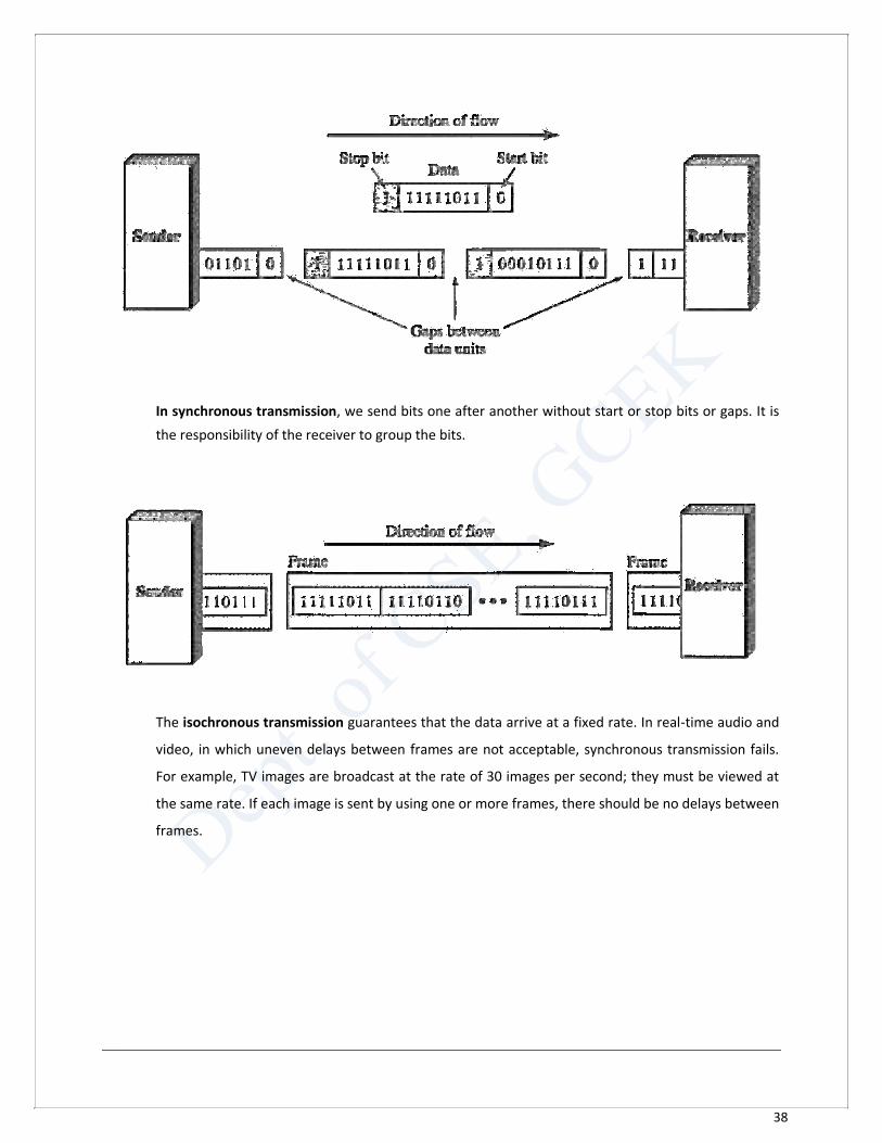
In asynchronous transmission, we send 1 start bit (0) at the beginning and 1 or more stop bits

(1) at the end of each byte. There may be a gap between each byte.

38

In synchronous transmission, we send bits one after another without start or stop bits or gaps. It is

the responsibility of the receiver to group the bits.

The isochronous transmission guarantees that the data arrive at a fixed rate. In real-time audio and

video, in which uneven delays between frames are not acceptable, synchronous transmission fails.

For example, TV images are broadcast at the rate of 30 images per second; they must be viewed at

the same rate. If each image is sent by using one or more frames, there should be no delays between

frames.

39

CHAPTER 5

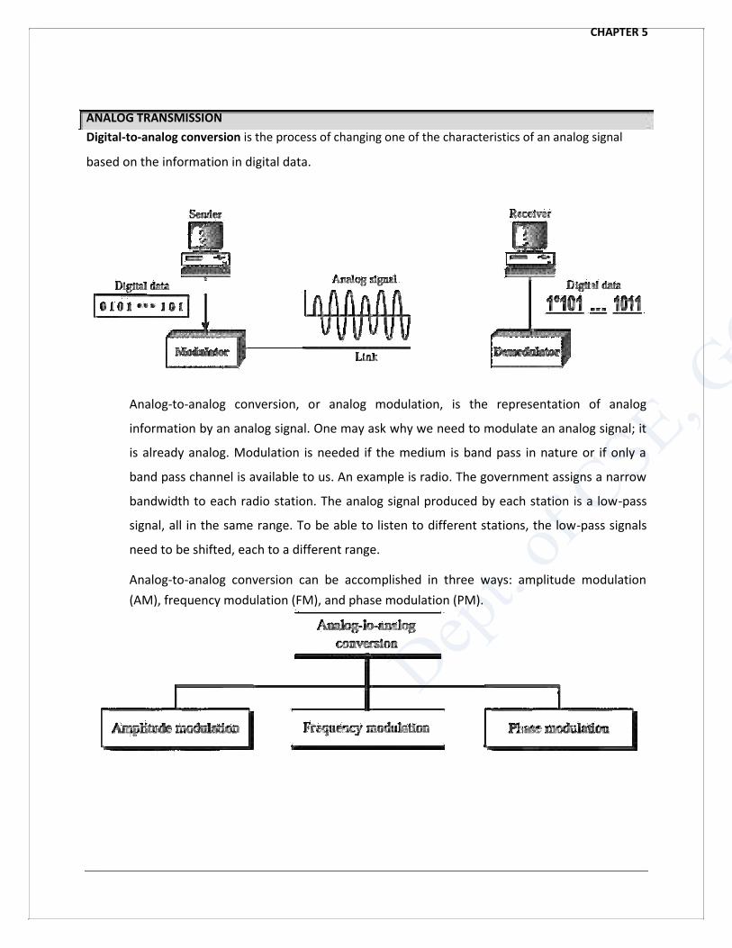
ANALOG TRANSMISSION Digital-to-analog conversion is the process of changing one of the characteristics of an analog signal based on the information in digital data.

Analog-to-analog conversion, or analog modulation, is the representation of analog

information by an analog signal. One may ask why we need to modulate an analog signal; it

is already analog. Modulation is needed if the medium is band pass in nature or if only a

band pass channel is available to us. An example is radio. The government assigns a narrow

bandwidth to each radio station. The analog signal produced by each station is a low-pass

signal, all in the same range. To be able to listen to different stations, the low-pass signals

need to be shifted, each to a different range.

Analog-to-analog conversion can be accomplished in three ways: amplitude modulation

(AM), frequency modulation (FM), and phase modulation (PM).

40

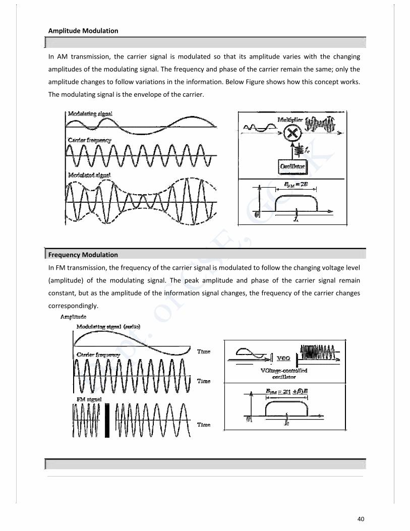
Amplitude Modulation

In AM transmission, the carrier signal is modulated so that its amplitude varies with the changing

amplitudes of the modulating signal. The frequency and phase of the carrier remain the same; only the

amplitude changes to follow variations in the information. Below Figure shows how this concept works.

The modulating signal is the envelope of the carrier.

Frequency Modulation In FM transmission, the frequency of the carrier signal is modulated to follow the changing voltage level

(amplitude) of the modulating signal. The peak amplitude and phase of the carrier signal remain

constant, but as the amplitude of the information signal changes, the frequency of the carrier changes

correspondingly.

41

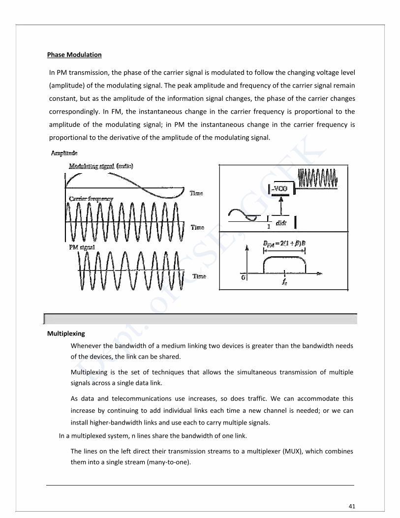
Phase Modulation

In PM transmission, the phase of the carrier signal is modulated to follow the changing voltage level

(amplitude) of the modulating signal. The peak amplitude and frequency of the carrier signal remain

constant, but as the amplitude of the information signal changes, the phase of the carrier changes

correspondingly. In FM, the instantaneous change in the carrier frequency is proportional to the

amplitude of the modulating signal; in PM the instantaneous change in the carrier frequency is

proportional to the derivative of the amplitude of the modulating signal.

Multiplexing

Whenever the bandwidth of a medium linking two devices is greater than the bandwidth needs

of the devices, the link can be shared.

Multiplexing is the set of techniques that allows the simultaneous transmission of multiple

signals across a single data link.

As data and telecommunications use increases, so does traffic. We can accommodate this

increase by continuing to add individual links each time a new channel is needed; or we can

install higher-bandwidth links and use each to carry multiple signals.

In a multiplexed system, n lines share the bandwidth of one link.

The lines on the left direct their transmission streams to a multiplexer (MUX), which combines

them into a single stream (many-to-one).

42

This page is left vacant intentionally

43

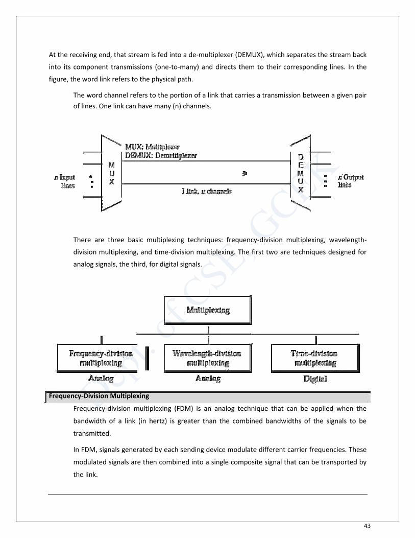
At the receiving end, that stream is fed into a de-multiplexer (DEMUX), which separates the stream back

into its component transmissions (one-to-many) and directs them to their corresponding lines. In the

figure, the word link refers to the physical path.

The word channel refers to the portion of a link that carries a transmission between a given pair

of lines. One link can have many (n) channels.

There are three basic multiplexing techniques: frequency-division multiplexing, wavelength-

division multiplexing, and time-division multiplexing. The first two are techniques designed for

analog signals, the third, for digital signals.

Frequency-Division Multiplexing

Frequency-division multiplexing (FDM) is an analog technique that can be applied when the

bandwidth of a link (in hertz) is greater than the combined bandwidths of the signals to be

transmitted.

In FDM, signals generated by each sending device modulate different carrier frequencies. These

modulated signals are then combined into a single composite signal that can be transported by

the link.

44

Carrier frequencies are separated by sufficient bandwidth to accommodate the modulated

signal.

These bandwidth ranges are the channels through which the various signals travel. Channels can

be separated by strips of unused bandwidth-guard bands-to prevent signals from overlapping.

In addition, carrier frequencies must not interfere with the original data frequencies.

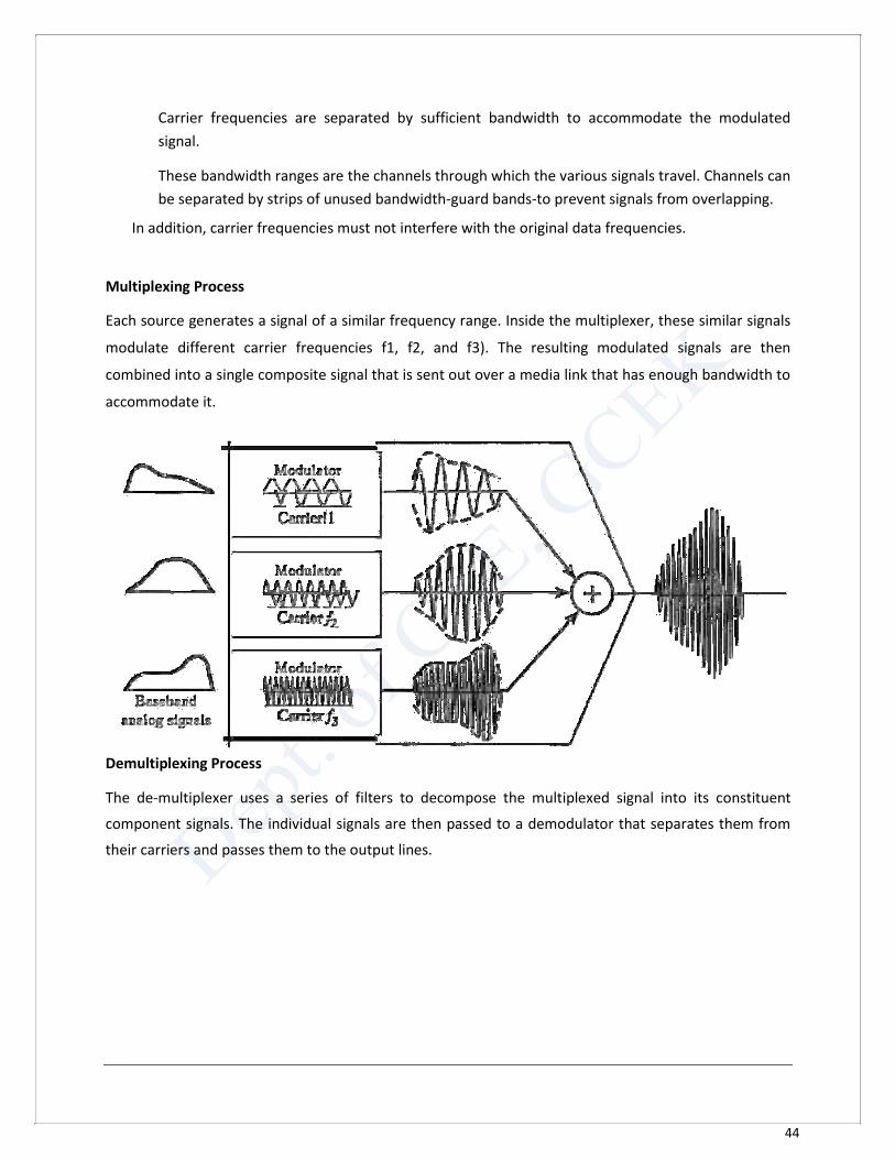
Multiplexing Process Each source generates a signal of a similar frequency range. Inside the multiplexer, these similar signals

modulate different carrier frequencies f1, f2, and f3). The resulting modulated signals are then

combined into a single composite signal that is sent out over a media link that has enough bandwidth to

accommodate it.

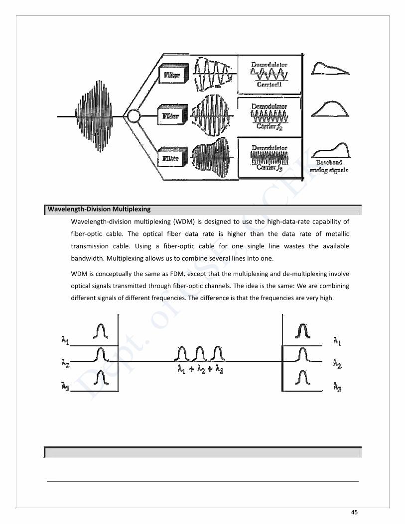
Demultiplexing Process The de-multiplexer uses a series of filters to decompose the multiplexed signal into its constituent

component signals. The individual signals are then passed to a demodulator that separates them from

their carriers and passes them to the output lines.

45

Wavelength-Division Multiplexing

Wavelength-division multiplexing (WDM) is designed to use the high-data-rate capability of

fiber-optic cable. The optical fiber data rate is higher than the data rate of metallic

transmission cable. Using a fiber-optic cable for one single line wastes the available

bandwidth. Multiplexing allows us to combine several lines into one.

WDM is conceptually the same as FDM, except that the multiplexing and de-multiplexing involve

optical signals transmitted through fiber-optic channels. The idea is the same: We are combining

different signals of different frequencies. The difference is that the frequencies are very high.

46

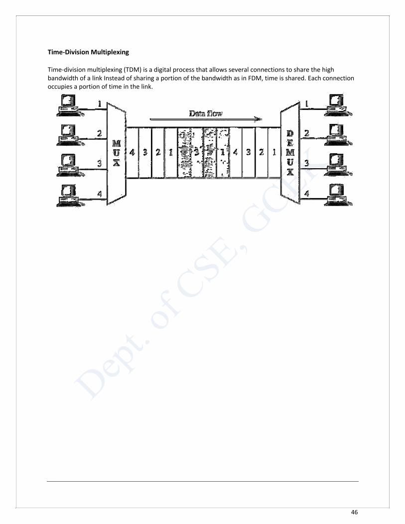
Time-Division Multiplexing Time-division multiplexing (TDM) is a digital process that allows several connections to share the high bandwidth of a link Instead of sharing a portion of the bandwidth as in FDM, time is shared. Each connection occupies a portion of time in the link.

47

CHAPTER 6 TRANSMISSION MEDIA

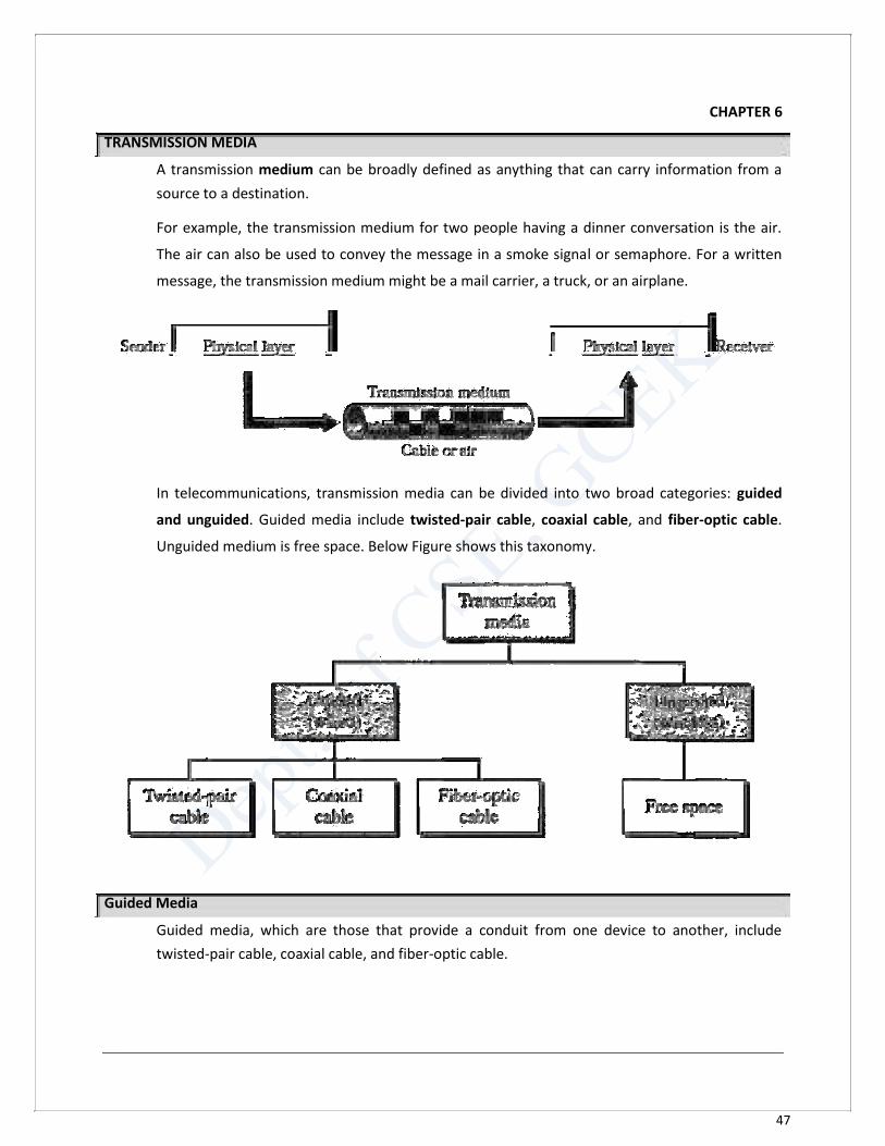
A transmission medium can be broadly defined as anything that can carry information from a

source to a destination.

For example, the transmission medium for two people having a dinner conversation is the air.

The air can also be used to convey the message in a smoke signal or semaphore. For a written

message, the transmission medium might be a mail carrier, a truck, or an airplane.

In telecommunications, transmission media can be divided into two broad categories: guided

and unguided. Guided media include twisted-pair cable, coaxial cable, and fiber-optic cable.

Unguided medium is free space. Below Figure shows this taxonomy.

Guided Media

Guided media, which are those that provide a conduit from one device to another, include

twisted-pair cable, coaxial cable, and fiber-optic cable.

48

A signal traveling along any of these media is directed and contained by the physical limits of the

medium. Twisted-pair and coaxial cable use metallic (copper) conductors that accept and

transport signals in the form of electric current.

Optical fiber is a cable that accepts and transports signals in the form of light.

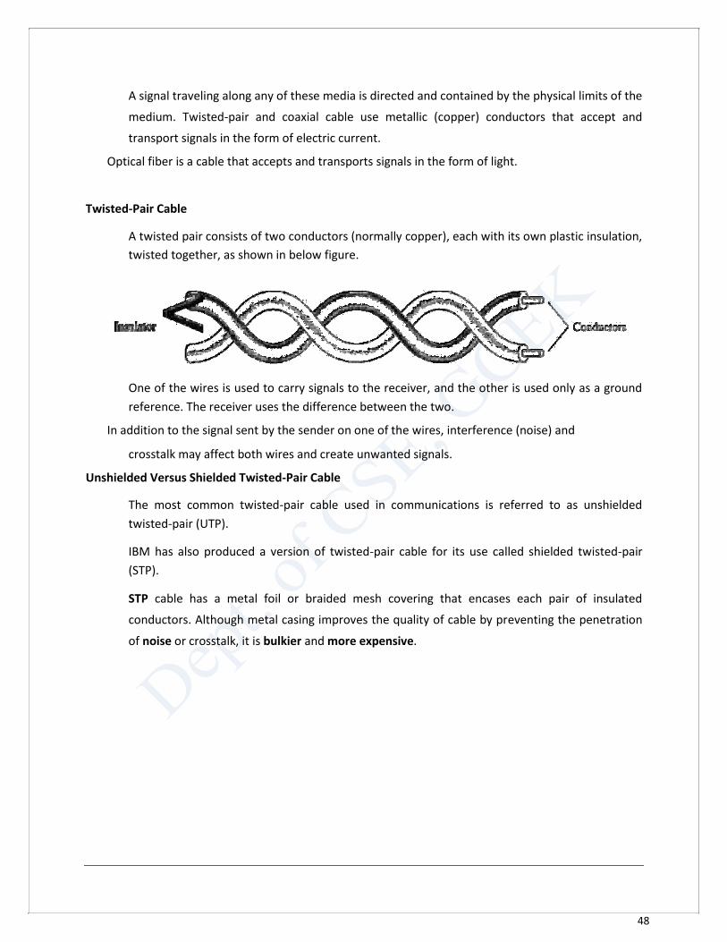
Twisted-Pair Cable

A twisted pair consists of two conductors (normally copper), each with its own plastic insulation,

twisted together, as shown in below figure.

One of the wires is used to carry signals to the receiver, and the other is used only as a ground

reference. The receiver uses the difference between the two.

In addition to the signal sent by the sender on one of the wires, interference (noise) and

crosstalk may affect both wires and create unwanted signals. Unshielded Versus Shielded Twisted-Pair Cable

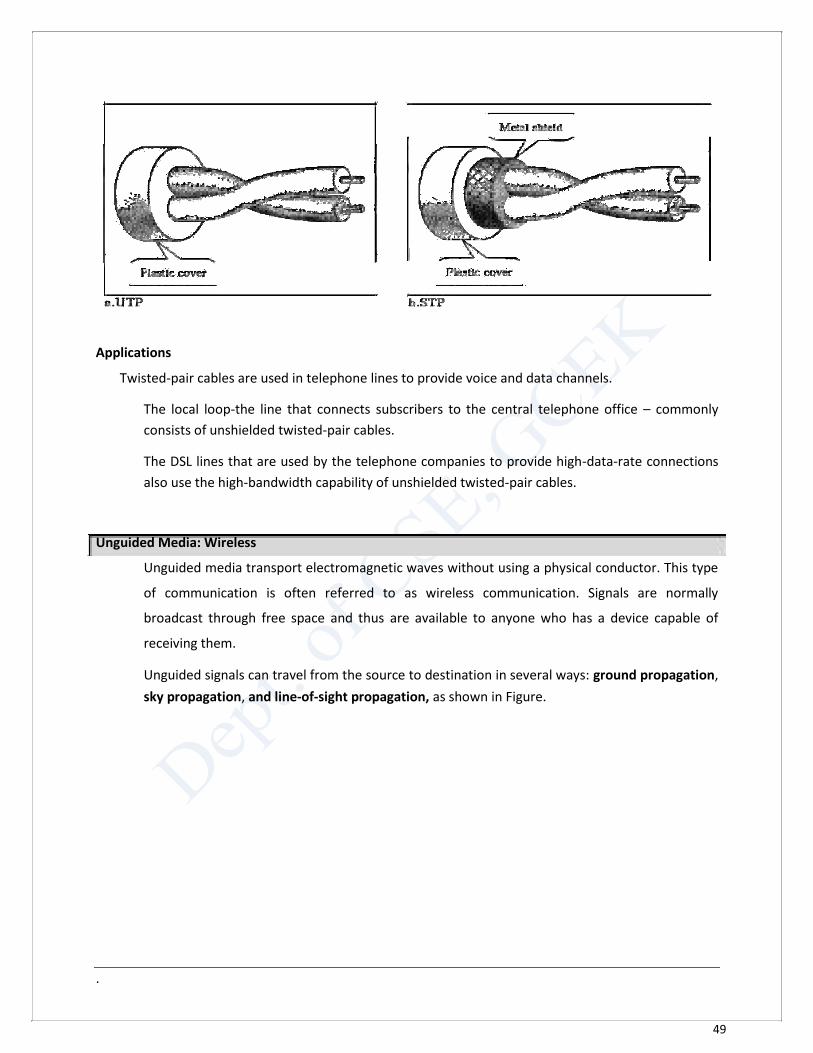
The most common twisted-pair cable used in communications is referred to as unshielded

twisted-pair (UTP).

IBM has also produced a version of twisted-pair cable for its use called shielded twisted-pair

(STP).

STP cable has a metal foil or braided mesh covering that encases each pair of insulated

conductors. Although metal casing improves the quality of cable by preventing the penetration

of noise or crosstalk, it is bulkier and more expensive.

49

Applications

Twisted-pair cables are used in telephone lines to provide voice and data channels.

The local loop-the line that connects subscribers to the central telephone office – commonly

consists of unshielded twisted-pair cables.

The DSL lines that are used by the telephone companies to provide high-data-rate connections

also use the high-bandwidth capability of unshielded twisted-pair cables.

Unguided Media: Wireless

Unguided media transport electromagnetic waves without using a physical conductor. This type

of communication is often referred to as wireless communication. Signals are normally

broadcast through free space and thus are available to anyone who has a device capable of

receiving them.

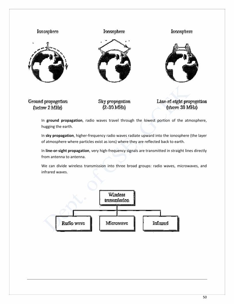
Unguided signals can travel from the source to destination in several ways: ground propagation,

sky propagation, and line-of-sight propagation, as shown in Figure.

.

50

In ground propagation, radio waves travel through the lowest portion of the atmosphere,

hugging the earth.

In sky propagation, higher-frequency radio waves radiate upward into the ionosphere (the layer

of atmosphere where particles exist as ions) where they are reflected back to earth.

In line-or-sight propagation, very high-frequency signals are transmitted in straight lines directly

from antenna to antenna.

We can divide wireless transmission into three broad groups: radio waves, microwaves, and

infrared waves.

51

Radio Waves

Although there is no clear-cut demarcation between radio waves and microwaves,

electromagnetic waves ranging in frequencies between 3 kHz and 1 GHz are normally called

radio waves; waves ranging in frequencies between 1 and 300 GHz are called microwaves.

Radio waves, for the most part, are omni-directional. When an antenna transmits radio waves,

they are propagated in all directions. This means that the sending and receiving antennas do not

have to be aligned.

The omni-directional property has a disadvantage, too. The radio waves transmitted by one

antenna are susceptible to interference by another antenna that may send signals using the

same frequency or band.

Radio waves, particularly those waves that propagate in the sky mode, can travel long distances.

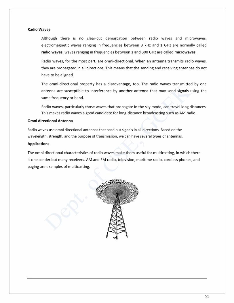
This makes radio waves a good candidate for long-distance broadcasting such as AM radio. Omni directional Antenna Radio waves use omni directional antennas that send out signals in all directions. Based on the

wavelength, strength, and the purpose of transmission, we can have several types of antennas. Applications The omni directional characteristics of radio waves make them useful for multicasting, in which there

is one sender but many receivers. AM and FM radio, television, maritime radio, cordless phones, and

paging are examples of multicasting.

52

Microwaves

Electromagnetic waves having frequencies between I and 300 GHz are called microwaves. Microwaves are unidirectional.

When an antenna transmits microwave waves, they can be narrowly focused. This means that

the sending and receiving antennas need to be aligned. The unidirectional property has an

obvious advantage. A pair of antennas can be aligned without interfering with another pair of

aligned antennas.

The following describes some characteristics of microwave propagation:

Microwave propagation is line-of-sight. Since the towers with the mounted antennas

need to be in direct sight of each other, towers that are far apart need to be very tall.

The curvatures of the earth as well as other blocking obstacles do not allow two short

towers to communicate by using microwaves. Repeaters are often needed for long

distance communication.

Very high-frequency microwaves cannot penetrate walls. This characteristic can be a

disadvantage if receivers are inside buildings.

The microwave band is relatively wide, almost 299 GHz. Therefore wider sub bands can

be assigned, and a high data rate is possible.

Use of certain portions of the band requires permission from authorities.

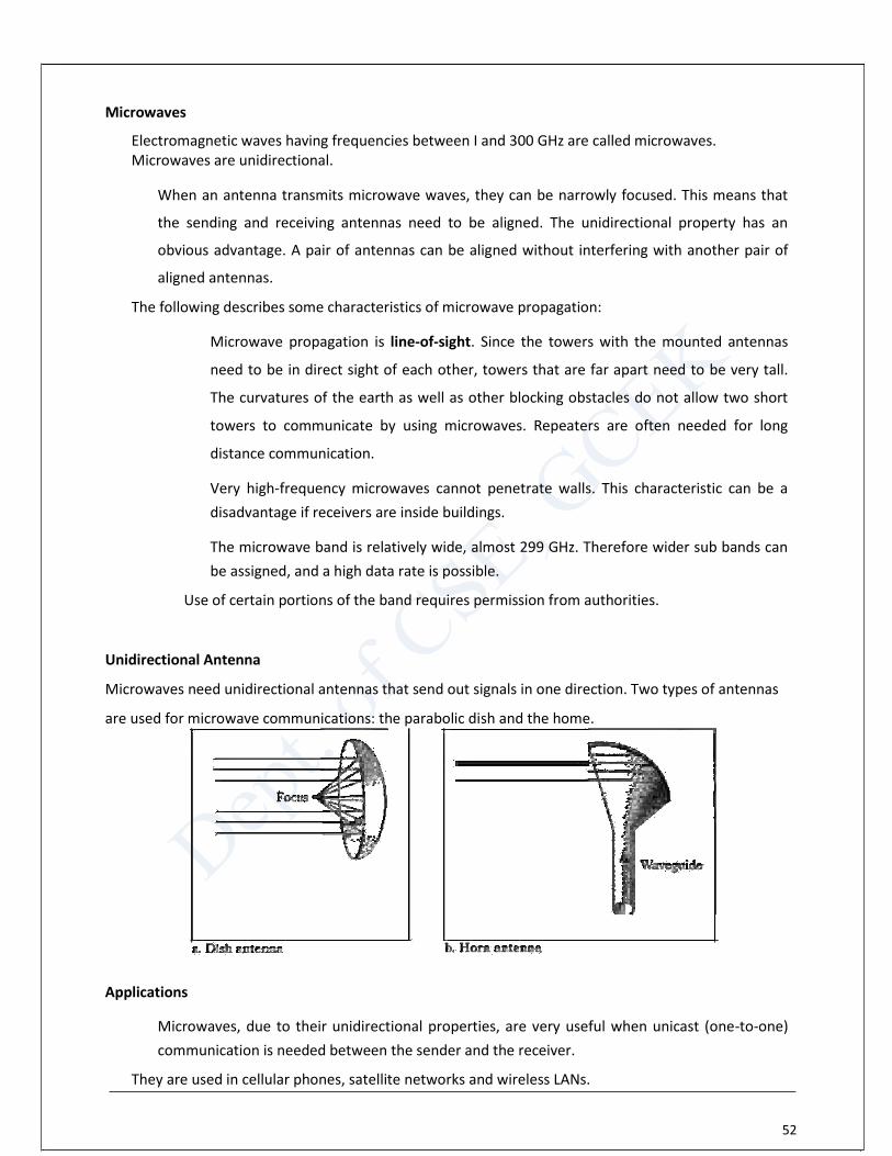
Unidirectional Antenna Microwaves need unidirectional antennas that send out signals in one direction. Two types of antennas are used for microwave communications: the parabolic dish and the home. Applications

Microwaves, due to their unidirectional properties, are very useful when unicast (one-to-one)

communication is needed between the sender and the receiver.

They are used in cellular phones, satellite networks and wireless LANs.

53

Infrared Infrared waves, with frequencies from 300 GHz to 400 THz (wavelengths from 1 mm to 770 nm), can be

used for short-range communication. Infrared waves, having high frequencies, cannot penetrate walls. Applications The infrared band, almost 400 THz, has an excellent potential for data transmission. Such a wide

bandwidth can be used to transmit digital data with a very high data rate.

54

CHAPTER 7 SWITCHING A switched network consists of a series of interlinked nodes, called switches. Switches are devices

capable of creating temporary connections between two or more devices linked to the switch. In a

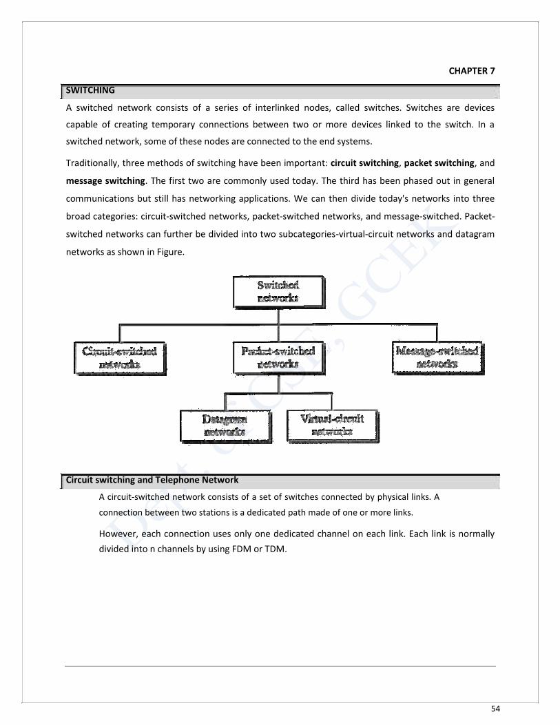
switched network, some of these nodes are connected to the end systems. Traditionally, three methods of switching have been important: circuit switching, packet switching, and

message switching. The first two are commonly used today. The third has been phased out in general

communications but still has networking applications. We can then divide today's networks into three

broad categories: circuit-switched networks, packet-switched networks, and message-switched. Packet-

switched networks can further be divided into two subcategories-virtual-circuit networks and datagram

networks as shown in Figure.

Circuit switching and Telephone Network

A circuit-switched network consists of a set of switches connected by physical links. A

connection between two stations is a dedicated path made of one or more links.

However, each connection uses only one dedicated channel on each link. Each link is normally

divided into n channels by using FDM or TDM.

55

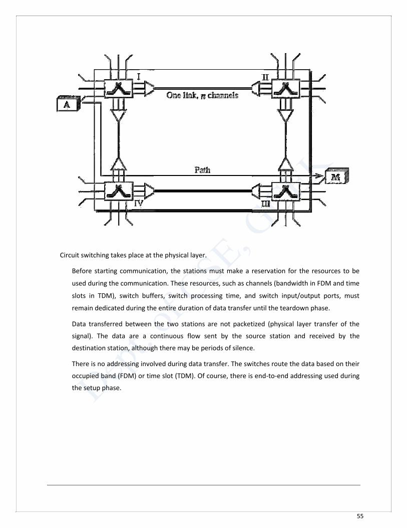
Circuit switching takes place at the physical layer.

Before starting communication, the stations must make a reservation for the resources to be

used during the communication. These resources, such as channels (bandwidth in FDM and time

slots in TDM), switch buffers, switch processing time, and switch input/output ports, must

remain dedicated during the entire duration of data transfer until the teardown phase.

Data transferred between the two stations are not packetized (physical layer transfer of the

signal). The data are a continuous flow sent by the source station and received by the

destination station, although there may be periods of silence.

There is no addressing involved during data transfer. The switches route the data based on their

occupied band (FDM) or time slot (TDM). Of course, there is end-to-end addressing used during

the setup phase.

56

Three Phases The actual communication in a circuit-switched network requires three phases: connection setup, data transfer, and connection teardown. Setup Phase Before the two parties (or multiple parties in a conference call) can communicate, a dedicated circuit

(combination of channels in links) needs to be established. The end systems are normally connected

through dedicated lines to the switches, so connection setup means creating dedicated channels

between the switches. Data Transfer Phase After the establishment of the dedicated circuit (channels), the two parties can transfer data. Teardown Phase When one of the parties needs to disconnect, a signal is sent to each switch to release the resources. Circuit-Switched Technology in Telephone Networks The telephone companies have previously chosen the circuit switched approach to switching in the

physical layer; today the tendency is moving toward other switching techniques. For example, the

telephone number is used as the global address, and a signaling system (called SS7) is used for the setup

and teardown phases.

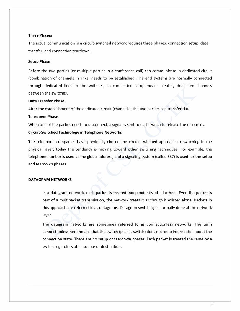
DATAGRAM NETWORKS

In a datagram network, each packet is treated independently of all others. Even if a packet is

part of a multipacket transmission, the network treats it as though it existed alone. Packets in

this approach are referred to as datagrams. Datagram switching is normally done at the network

layer.

The datagram networks are sometimes referred to as connectionless networks. The term

connectionless here means that the switch (packet switch) does not keep information about the

connection state. There are no setup or teardown phases. Each packet is treated the same by a

switch regardless of its source or destination.

57

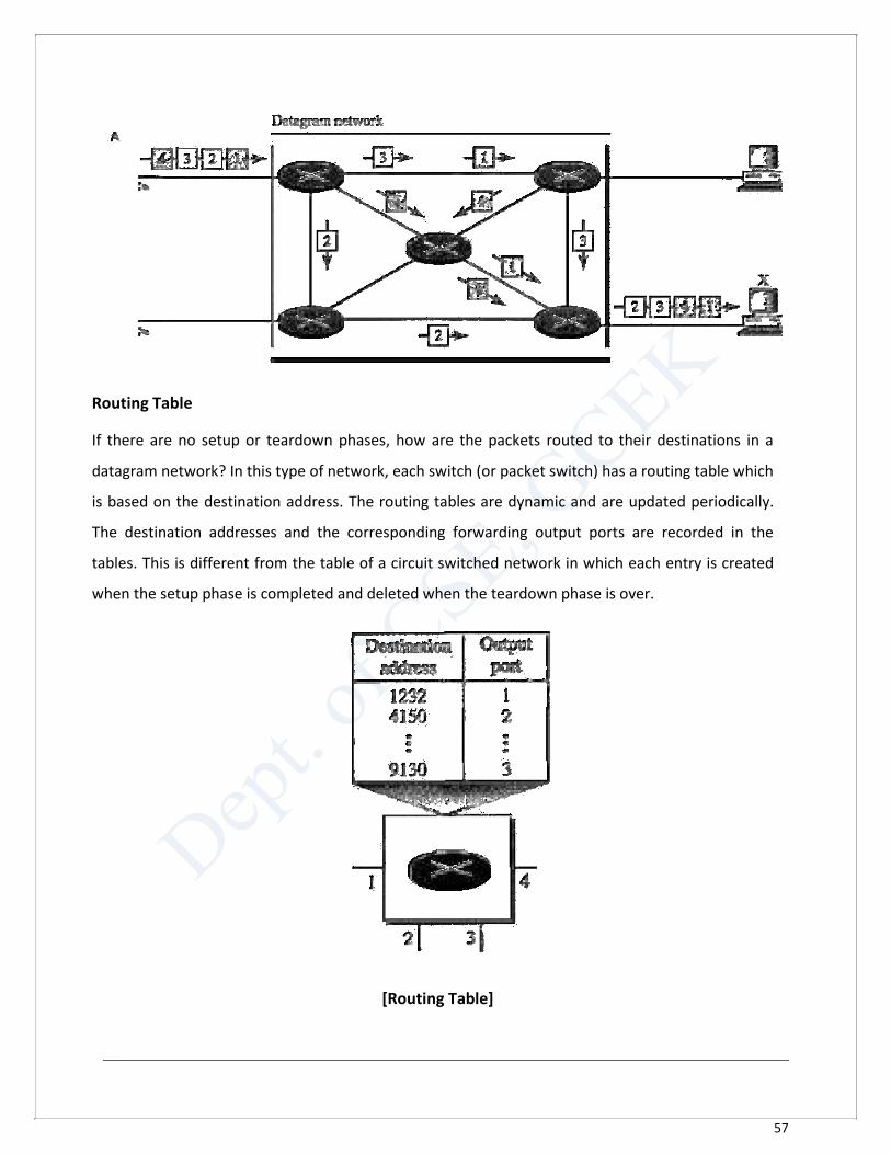
Routing Table If there are no setup or teardown phases, how are the packets routed to their destinations in a

datagram network? In this type of network, each switch (or packet switch) has a routing table which

is based on the destination address. The routing tables are dynamic and are updated periodically.

The destination addresses and the corresponding forwarding output ports are recorded in the

tables. This is different from the table of a circuit switched network in which each entry is created

when the setup phase is completed and deleted when the teardown phase is over.

[Routing Table]

58

Destination Address Every packet in a datagram network carries a header that contains, among other information, the

destination address of the packet. When the switch receives the packet, this destination address is

examined; the routing table is consulted to find the corresponding port through which the packet should

be forwarded. This address, unlike the address in a virtual-circuit-switched network, remains the same

during the entire journey of the packet. Efficiency The efficiency of a datagram network is better than that of a circuit-switched network; resources are

allocated only when there are packets to be transferred. If a source sends a packet and there is a delay

of a few minutes before another packet can be sent, the resources can be reallocated during these

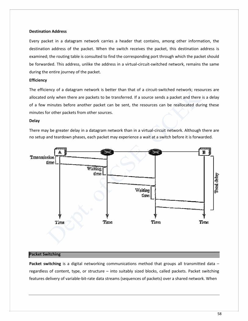
minutes for other packets from other sources. Delay There may be greater delay in a datagram network than in a virtual-circuit network. Although there are

no setup and teardown phases, each packet may experience a wait at a switch before it is forwarded.

Packet Switching Packet switching is a digital networking communications method that groups all transmitted data –

regardless of content, type, or structure – into suitably sized blocks, called packets. Packet switching

features delivery of variable-bit-rate data streams (sequences of packets) over a shared network. When

59

traversing network adapters, switches, routers and other network nodes, packets are buffered and

queued, resulting in variable delay and throughput depending on the traffic load in the network.

Packet switching contrasts with another principal networking paradigm, circuit switching, a method

which sets up a limited number of dedicated connections of constant bit rate and constant delay

between nodes for exclusive use during the communication session. In case of traffic fees (as opposed

to flat rate), for example in cellular communication services, circuit switching is characterized by a fee

per time unit of connection time, even when no data is transferred, while packet switching is

characterized by a fee per unit of information.

Two major packet switching modes exist: (1) Connectionless packet switching, also known as datagram switching, and (2) Connection-oriented packet switching, also known as virtual circuit switching.

In the first case each packet includes complete addressing or routing information. The packets are

routed individually, sometimes resulting in different paths and out-of-order delivery.

In the second case a connection is defined and preallocated in each involved node during a connection

phase before any packet is transferred.

60

CHAPTER 8 ERROR DETECTION AND CORRECTION Data can be corrupted during transmission. Some applications require that errors be detected and

corrected. Types of Errors Whenever bits flow from one point to another, they are subject to unpredictable changes because of

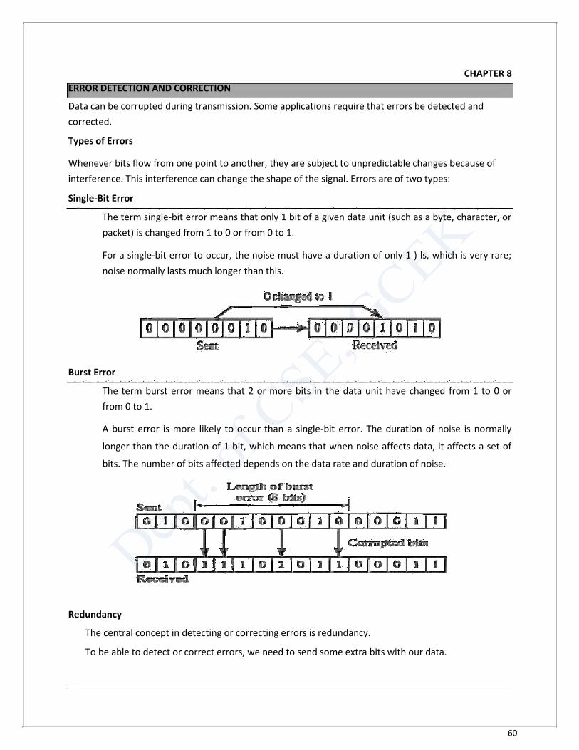
interference. This interference can change the shape of the signal. Errors are of two types: Single-Bit Error

The term single-bit error means that only 1 bit of a given data unit (such as a byte, character, or

packet) is changed from 1 to 0 or from 0 to 1.

For a single-bit error to occur, the noise must have a duration of only 1 ) ls, which is very rare;

noise normally lasts much longer than this.

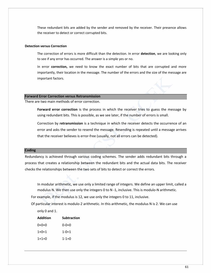
Burst Error

The term burst error means that 2 or more bits in the data unit have changed from 1 to 0 or

from 0 to 1.

A burst error is more likely to occur than a single-bit error. The duration of noise is normally

longer than the duration of 1 bit, which means that when noise affects data, it affects a set of

bits. The number of bits affected depends on the data rate and duration of noise.

Redundancy

The central concept in detecting or correcting errors is redundancy.

To be able to detect or correct errors, we need to send some extra bits with our data.

61

These redundant bits are added by the sender and removed by the receiver. Their presence allows

the receiver to detect or correct corrupted bits.

Detection versus Correction

The correction of errors is more difficult than the detection. In error detection, we are looking only

to see if any error has occurred. The answer is a simple yes or no.

In error correction, we need to know the exact number of bits that are corrupted and more

importantly, their location in the message. The number of the errors and the size of the message are

important factors.

Forward Error Correction versus Retransmission There are two main methods of error correction.

Forward error correction is the process in which the receiver tries to guess the message by

using redundant bits. This is possible, as we see later, if the number of errors is small.

Correction by retransmission is a technique in which the receiver detects the occurrence of an

error and asks the sender to resend the message. Resending is repeated until a message arrives

that the receiver believes is error-free (usually, not all errors can be detected).

Coding Redundancy is achieved through various coding schemes. The sender adds redundant bits through a

process that creates a relationship between the redundant bits and the actual data bits. The receiver

checks the relationships between the two sets of bits to detect or correct the errors.

In modular arithmetic, we use only a limited range of integers. We define an upper limit, called a

modulus N. We then use only the integers 0 to N -1, inclusive. This is modulo-N arithmetic.

For example, if the modulus is 12, we use only the integers 0 to 11, inclusive.

Of particular interest is modulo-2 arithmetic. In this arithmetic, the modulus N is 2. We can use

only 0 and 1.

Addition Subtraction

0+0=0 0-0=0

1+0=1 1-0=1

1+1=0 1-1=0

62

0+1=1 0-1=1

Particularly that addition and subtraction give the same results. In this arithmetic we use the XOR

(exclusive OR) operation for both addition and subtraction. The result of an XOR operation is 0 if two

bits are the same; the result is 1 if two bits are different.

If the modulus is not 2, addition and subtraction are distinct.

BLOCK CODING

In block coding, we divide our message into blocks, each of k bits, called data words. We add r

redundant bits to each block to make the length n = k + r. The resulting n-bit blocks are called

code words.

With k bits, we can create a combination of 2k data words; with n bits, we can create a

combination of 2n code words. Since n > k, the number of possible code words is larger than the

number of possible data words. The block coding process is one-to-one; the same data word is

always encoded as the same codeword. This means that we have 2n - 2k code words that are

not used.

Error Detection The sender creates code words out of data words by using a generator that applies the rules and

procedures of encoding. Each codeword sent to the receiver may change during transmission. If the

received codeword is the same as one of the valid code words, the word is accepted; the corresponding

data word is extracted for use. If the received codeword is not valid, it is discarded. However, if the

codeword is corrupted during transmission but the received word still matches a valid codeword, the

error remains undetected. This type of coding can detect only single errors. Two or more errors may

remain undetected.

63

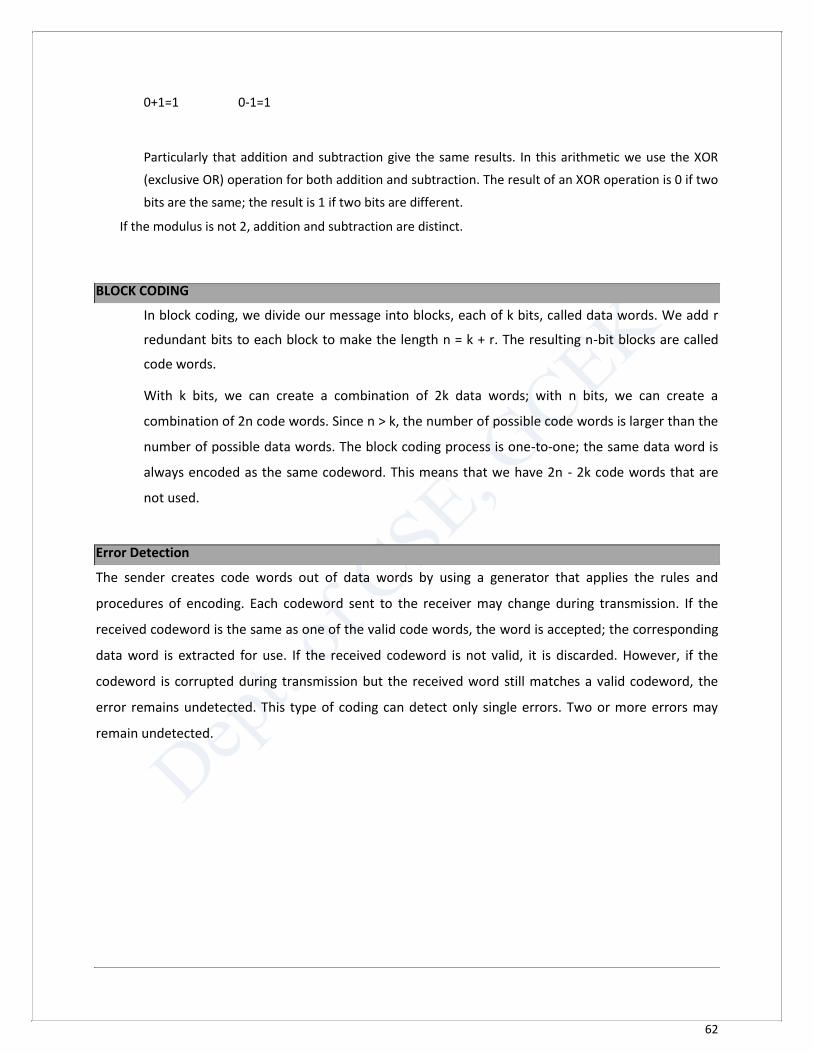
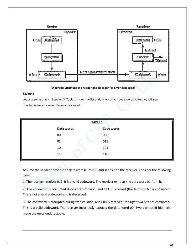
[Diagram: Structure of encoder and decoder for Error detection]

Example Let us assume that k =2 and n =3. Table 1 shows the list of data words and code words. Later, we will see how to derive a codeword from a data word.

TABLE 1

Data words Code words

00 000

01 011

10 101

11 110

Assume the sender encodes the data word 01 as 011 and sends it to the receiver. Consider the following

cases: 1. The receiver receives 011. It is a valid codeword. The receiver extracts the data word 01 from it. 2. The codeword is corrupted during transmission, and 111 is received (the leftmost bit is corrupted).

This is not a valid codeword and is discarded. 3. The codeword is corrupted during transmission, and 000 is received (the right two bits are corrupted).

This is a valid codeword. The receiver incorrectly extracts the data word 00. Two corrupted bits have

made the error undetectable.

64

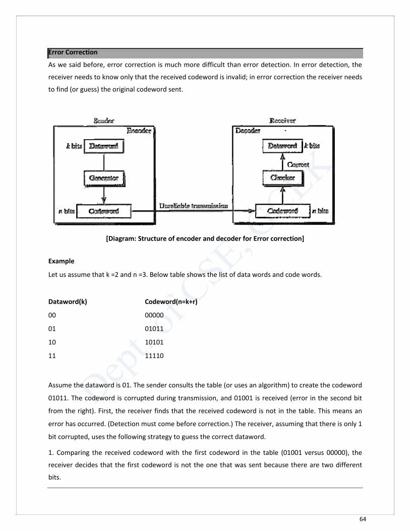
Error Correction As we said before, error correction is much more difficult than error detection. In error detection, the

receiver needs to know only that the received codeword is invalid; in error correction the receiver needs

to find (or guess) the original codeword sent.

[Diagram: Structure of encoder and decoder for Error correction] Example Let us assume that k =2 and n =3. Below table shows the list of data words and code words.

Dataword(k) Codeword(n=k+r)

00 00000

01 01011

10 10101

11 11110 Assume the dataword is 01. The sender consults the table (or uses an algorithm) to create the codeword

01011. The codeword is corrupted during transmission, and 01001 is received (error in the second bit

from the right). First, the receiver finds that the received codeword is not in the table. This means an

error has occurred. (Detection must come before correction.) The receiver, assuming that there is only 1

bit corrupted, uses the following strategy to guess the correct dataword. 1. Comparing the received codeword with the first codeword in the table (01001 versus 00000), the

receiver decides that the first codeword is not the one that was sent because there are two different

bits.

65

2. By the same reasoning, the original codeword cannot be the third or fourth one in the table. 3. The original codeword must be the second one in the table because this is the only one that differs

from the received codeword by 1 bit. The receiver replaces 01001 with 01011 and consults the table to

find the dataword 01.

Hamming Distance

The Hamming distance between two words (of the same size) is the number of differences

between the corresponding bits.

The Hamming distance can easily be found if we apply the XOR operation on the two words and

count the number of 1s in the result. Note that the Hamming distance is a value greater than

zero.

The minimum Hamming distance is the smallest Hamming distance between all possible pairs in

a set of words.

Example: Let us find the Hamming distance between two pairs of words. 1. The Hamming distance d (000, 011) is 2 because 000 XOR 011 is 011 (two 1s). 2. The Hamming distance d (10101, 11110) is 3 because 10101 XOR 11110 is 01011 (three 1s).

Linear Block Codes

In a linear block code, the exclusive OR (XOR) of any two valid code words creates another valid

codeword.

The scheme in Table 1 is a linear block code because the result of XORing any codeword with

any other codeword is a valid codeword. For example, the XORing of the second and third code

words creates the fourth one.

Let us now show some linear block codes. These codes are trivial because we can easily find the

encoding and decoding algorithms and check their performances.

66

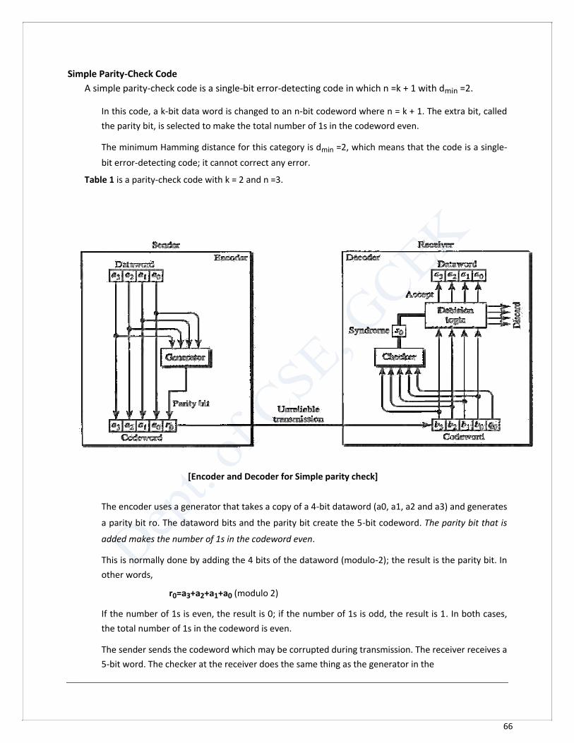
Simple Parity-Check Code

A simple parity-check code is a single-bit error-detecting code in which n =k + 1 with dmin =2.

In this code, a k-bit data word is changed to an n-bit codeword where n = k + 1. The extra bit, called

the parity bit, is selected to make the total number of 1s in the codeword even.

The minimum Hamming distance for this category is dmin =2, which means that the code is a single-

bit error-detecting code; it cannot correct any error.

Table 1 is a parity-check code with k = 2 and n =3.

[Encoder and Decoder for Simple parity check]

The encoder uses a generator that takes a copy of a 4-bit dataword (a0, a1, a2 and a3) and generates

a parity bit ro. The dataword bits and the parity bit create the 5-bit codeword. The parity bit that is

added makes the number of 1s in the codeword even.

This is normally done by adding the 4 bits of the dataword (modulo-2); the result is the parity bit. In

other words,

r0=a3+a2+a1+a0 (modulo 2)

If the number of 1s is even, the result is 0; if the number of 1s is odd, the result is 1. In both cases,

the total number of 1s in the codeword is even.

The sender sends the codeword which may be corrupted during transmission. The receiver receives a

5-bit word. The checker at the receiver does the same thing as the generator in the

67

sender with one exception: The addition is done over all 5 bits. The result, which is called the

syndrome, is just 1 bit. The syndrome is 0 when the number of 1s in the received codeword is

even; otherwise, it is 1.

s0=b3+b2+b1+b0 (modulo 2)

The syndrome is passed to the decision logic analyzer. If the syndrome is 0, there is no error in the

received codeword; the data portion of the received codeword is accepted as the dataword; if the

syndrome is 1, the data portion of the received codeword is discarded. The dataword is not created.

Example: Let us look at some transmission scenarios. Assume the sender sends the dataword 1011. The codeword created from this dataword is 10111, which is sent to the receiver. We examine five cases: 1. No error occurs; the received codeword is 10111. The syndrome is 0. The dataword 1011 is created.

2. One single-bit error changes a1. The received codeword is 10011. The syndrome is 1. No dataword is

created. 3. One single-bit error changes ro.The received codeword is 10110. The syndrome is 1. No dataword is

created. 4. An error changes ro and a second error changes a3. The received codeword is 00110. The

syndrome is 0. The dataword 0011 is created at the receiver. Note that here the dataword is wrongly created

due to the syndrome value. The simple parity-check decoder cannot detect an even number of errors. The

errors cancel each other out and give the syndrome a value of 0. 5. Three bits-a3, a2, and a1-are changed by errors. The received codeword is 01011. The syndrome is 1. The

dataword is not created. This shows that the simple parity check, guaranteed to detect one single error, can

also find any odd number of errors.

Hamming Code

These codes were originally designed with d min = 3, which means that they can detect up to two

errors or correct one single error. Although there are some Hamming codes that can correct

more than one error, our discussion focuses on the single-bit error-correcting code.

Let us find the relationship between n and k in a Hamming code. We need to choose an integer m >= 3.

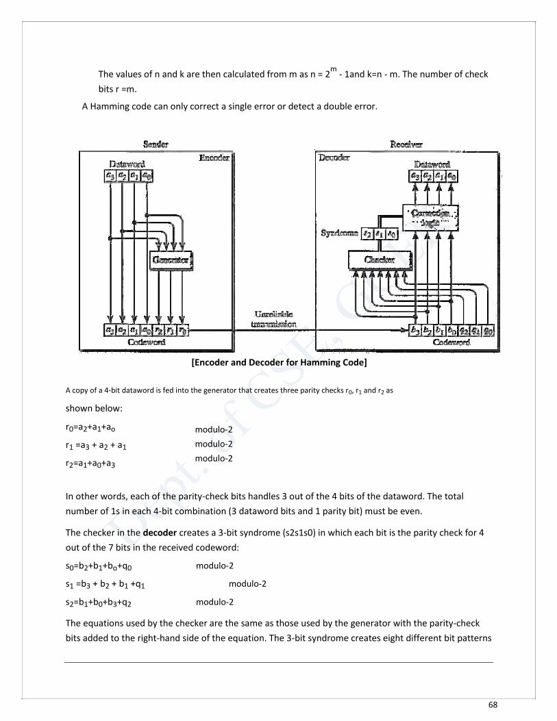
68

The values of n and k are then calculated from m as n = 2

m - 1and k=n - m. The number of check

bits r =m.

A Hamming code can only correct a single error or detect a double error.

[Encoder and Decoder for Hamming Code]

A copy of a 4-bit dataword is fed into the generator that creates three parity checks r0, r1 and r2 as shown below:

r0=a2+a1+ao

r1 =a3 + a2 + a1

r2=a1+a0+a3 In other words, each of the parity-check bits handles 3 out of the 4 bits of the dataword. The total

number of 1s in each 4-bit combination (3 dataword bits and 1 parity bit) must be even. The checker in the decoder creates a 3-bit syndrome (s2s1s0) in which each bit is the parity check for 4

out of the 7 bits in the received codeword: s0=b2+b1+bo+q0 modulo-2

s1 =b3 + b2 + b1 +q1 modulo-2

s2=b1+b0+b3+q2 modulo-2 The equations used by the checker are the same as those used by the generator with the parity-check

bits added to the right-hand side of the equation. The 3-bit syndrome creates eight different bit patterns

modulo-2

modulo-2

modulo-2

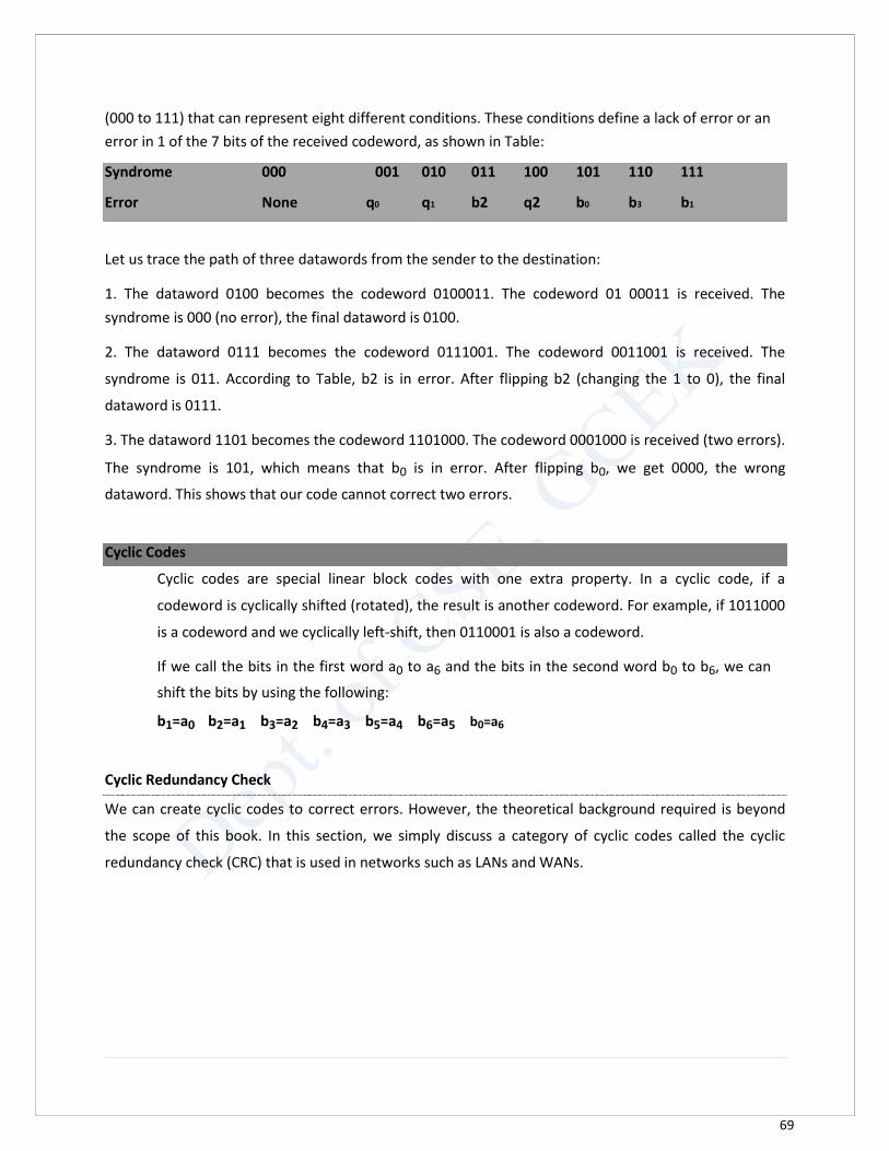
69

(000 to 111) that can represent eight different conditions. These conditions define a lack of error or an

error in 1 of the 7 bits of the received codeword, as shown in Table: Syndrome 000 001 010 011 100 101 110 111

Error None q0 q1 b2 q2 b0 b3 b1

Let us trace the path of three datawords from the sender to the destination: 1. The dataword 0100 becomes the codeword 0100011. The codeword 01 00011 is received. The

syndrome is 000 (no error), the final dataword is 0100. 2. The dataword 0111 becomes the codeword 0111001. The codeword 0011001 is received. The

syndrome is 011. According to Table, b2 is in error. After flipping b2 (changing the 1 to 0), the final

dataword is 0111. 3. The dataword 1101 becomes the codeword 1101000. The codeword 0001000 is received (two errors).

The syndrome is 101, which means that b0 is in error. After flipping b0, we get 0000, the wrong

dataword. This shows that our code cannot correct two errors.

Cyclic Codes

Cyclic codes are special linear block codes with one extra property. In a cyclic code, if a

codeword is cyclically shifted (rotated), the result is another codeword. For example, if 1011000

is a codeword and we cyclically left-shift, then 0110001 is also a codeword.

If we call the bits in the first word a0 to a6 and the bits in the second word b0 to b6, we can

shift the bits by using the following:

b1=a0 b2=a1 b3=a2 b4=a3 b5=a4 b6=a5 b0=a6

Cyclic Redundancy Check We can create cyclic codes to correct errors. However, the theoretical background required is beyond

the scope of this book. In this section, we simply discuss a category of cyclic codes called the cyclic

redundancy check (CRC) that is used in networks such as LANs and WANs.

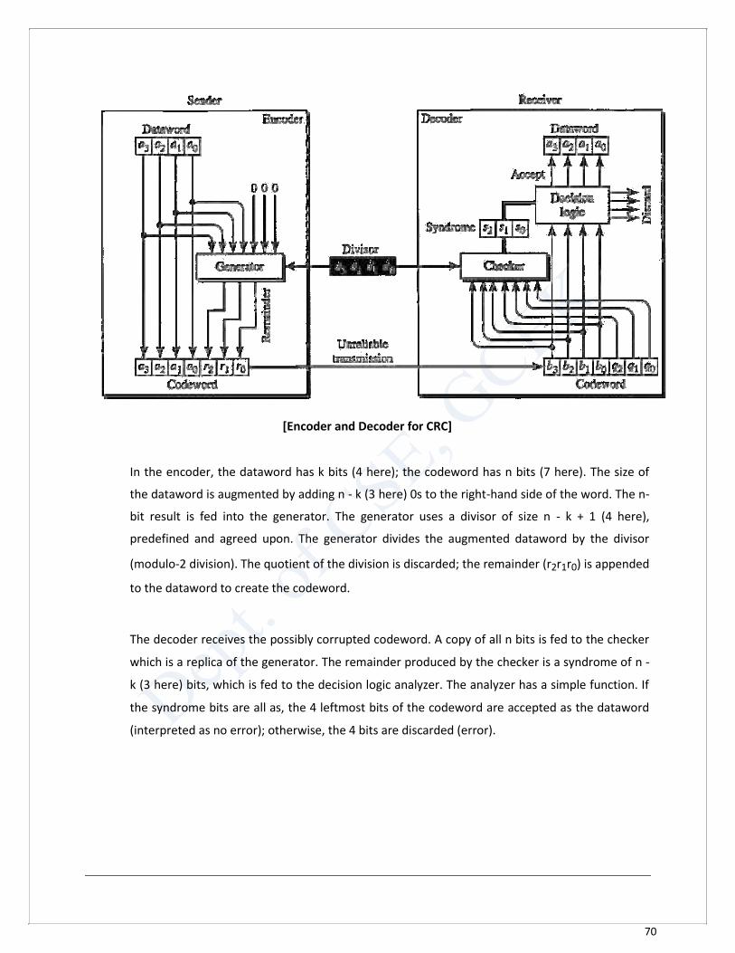
70

[Encoder and Decoder for CRC]

In the encoder, the dataword has k bits (4 here); the codeword has n bits (7 here). The size of

the dataword is augmented by adding n - k (3 here) 0s to the right-hand side of the word. The n-

bit result is fed into the generator. The generator uses a divisor of size n - k + 1 (4 here),

predefined and agreed upon. The generator divides the augmented dataword by the divisor

(modulo-2 division). The quotient of the division is discarded; the remainder (r2r1r0) is appended

to the dataword to create the codeword.

The decoder receives the possibly corrupted codeword. A copy of all n bits is fed to the checker

which is a replica of the generator. The remainder produced by the checker is a syndrome of n -

k (3 here) bits, which is fed to the decision logic analyzer. The analyzer has a simple function. If

the syndrome bits are all as, the 4 leftmost bits of the codeword are accepted as the dataword

(interpreted as no error); otherwise, the 4 bits are discarded (error).

71

Polynomial

A pattern of 0s and 1s can be represented as a polynomial with coefficients of 0 and 1. The power of each term shows the

position of the bit; the coefficient shows the value of the bit. Below figure shows a binary pattern and its polynomial

representation.

72

Chapter 9 DATA LINK CONTROL

The two main functions of the data link layer are data link control and media access control.

The first, data link control, deals with the design and procedures for communication between

two adjacent nodes: node-to-node communication.

The second function of the data link layer is media access control, or how to share the link.

Data link control functions include framing, flow and error control, and software implemented

protocols that provide smooth and reliable transmission of frames between nodes.

Framing

The data link layer, on the other hand, needs to pack bits into frames, so that each frame is

distinguishable from another.

Framing in the data link layer separates a message from one source to a destination, or from

other messages to other destinations, by adding a sender address and a destination address.

The destination address defines where the packet is to go; the sender address helps the

recipient acknowledge the receipt. Frames can be of fixed or variable size.

1. Fixed-Size Framing

In fixed-size framing, there is no need for defining the boundaries of the frames; the size itself can

be used as a delimiter.

2. Variable-Size Framing

In variable-size framing, we need a way to define the end of the frame and the beginning of the

next. Historically, two approaches were used for this purpose: a character-oriented approach and a

bit-oriented approach.

Character-Oriented Protocols In a character-oriented protocol, data to be carried are 8-bit characters.

The header, which normally carries the source and destination addresses and other control

information, and the trailer, which carries error detection or error correction redundant bits, are

also multiples of 8 bits.

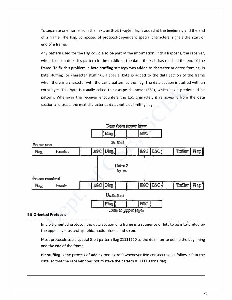
73

To separate one frame from the next, an 8-bit (I-byte) flag is added at the beginning and the end

of a frame. The flag, composed of protocol-dependent special characters, signals the start or

end of a frame.

Any pattern used for the flag could also be part of the information. If this happens, the receiver,

when it encounters this pattern in the middle of the data, thinks it has reached the end of the

frame. To fix this problem, a byte-stuffing strategy was added to character-oriented framing. In

byte stuffing (or character stuffing), a special byte is added to the data section of the frame

when there is a character with the same pattern as the flag. The data section is stuffed with an

extra byte. This byte is usually called the escape character (ESC), which has a predefined bit

pattern. Whenever the receiver encounters the ESC character, it removes it from the data

section and treats the next character as data, not a delimiting flag.

Bit-Oriented Protocols

In a bit-oriented protocol, the data section of a frame is a sequence of bits to be interpreted by

the upper layer as text, graphic, audio, video, and so on.

Most protocols use a special 8-bit pattern flag 01111110 as the delimiter to define the beginning

and the end of the frame.

Bit stuffing is the process of adding one extra 0 whenever five consecutive 1s follow a 0 in the

data, so that the receiver does not mistake the pattern 0111110 for a flag.

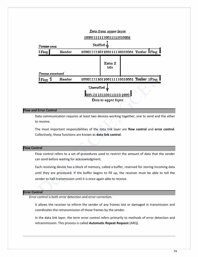
74

Flow and Error Control

Data communication requires at least two devices working together, one to send and the other

to receive.

The most important responsibilities of the data link layer are flow control and error control.

Collectively, these functions are known as data link control.

Flow Control

Flow control refers to a set of procedures used to restrict the amount of data that the sender

can send before waiting for acknowledgment.

Each receiving device has a block of memory, called a buffer, reserved for storing incoming data

until they are processed. If the buffer begins to fill up, the receiver must be able to tell the

sender to halt transmission until it is once again able to receive.

Error Control

Error control is both error detection and error correction.

It allows the receiver to inform the sender of any frames lost or damaged in transmission and

coordinates the retransmission of those frames by the sender.

In the data link layer, the term error control refers primarily to methods of error detection and

retransmission. This process is called Automatic Repeat Request (ARQ).

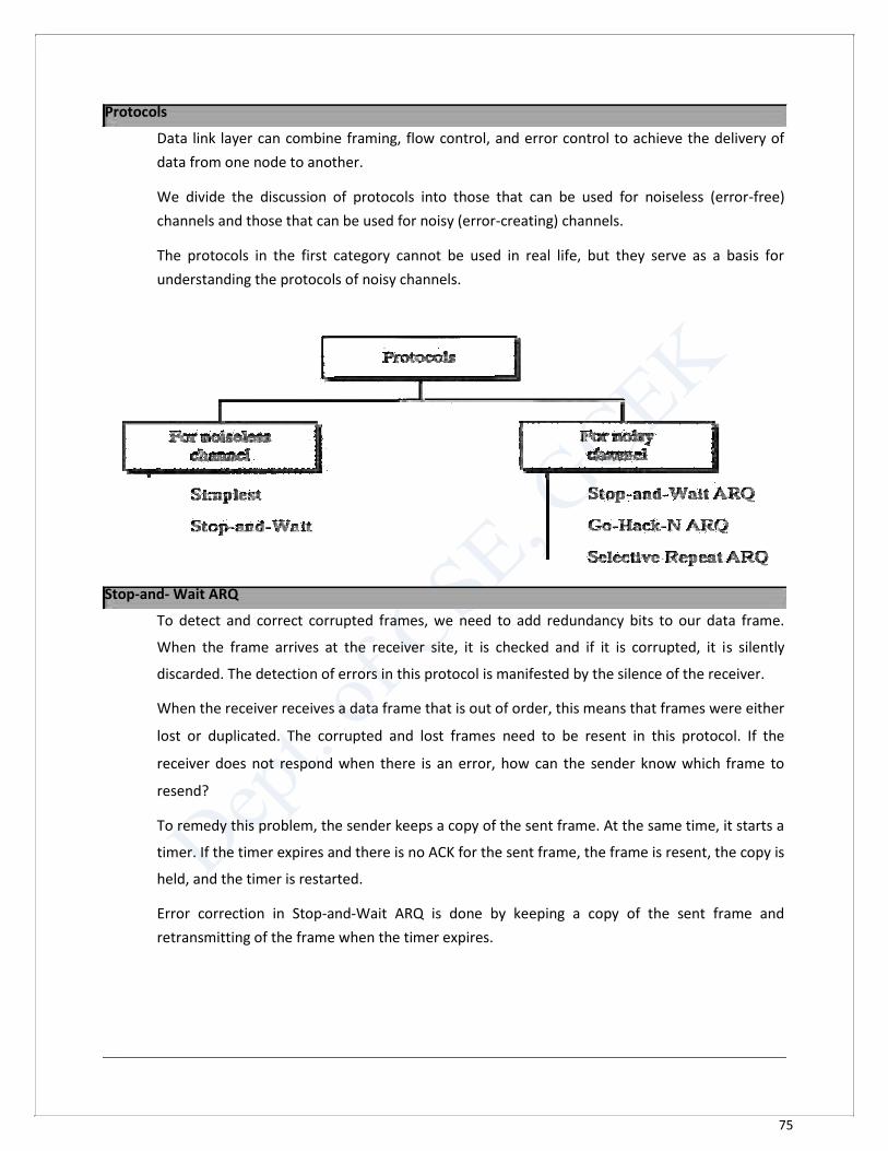
75

Protocols

Data link layer can combine framing, flow control, and error control to achieve the delivery of

data from one node to another.

We divide the discussion of protocols into those that can be used for noiseless (error-free)

channels and those that can be used for noisy (error-creating) channels.

The protocols in the first category cannot be used in real life, but they serve as a basis for

understanding the protocols of noisy channels.

Stop-and- Wait ARQ

To detect and correct corrupted frames, we need to add redundancy bits to our data frame.

When the frame arrives at the receiver site, it is checked and if it is corrupted, it is silently

discarded. The detection of errors in this protocol is manifested by the silence of the receiver.

When the receiver receives a data frame that is out of order, this means that frames were either

lost or duplicated. The corrupted and lost frames need to be resent in this protocol. If the

receiver does not respond when there is an error, how can the sender know which frame to

resend?

To remedy this problem, the sender keeps a copy of the sent frame. At the same time, it starts a

timer. If the timer expires and there is no ACK for the sent frame, the frame is resent, the copy is

held, and the timer is restarted.

Error correction in Stop-and-Wait ARQ is done by keeping a copy of the sent frame and

retransmitting of the frame when the timer expires.

76

Sequence Numbers

A frame is numbered by sequence numbers. A field is added to the data frame to hold the sequence number of that frame.

If we decide that the field is m bits long, the sequence numbers start from 0, go to 2m

- 1, and

then are repeated. Let us consider three cases: 1. The frame arrives safe and sound at the receiver site; the receiver sends an acknowledgment. The

acknowledgment arrives at the sender site, causing the sender to send the next frame numbered x + 1. 2. The frame arrives safe and sound at the receiver site; the receiver sends an acknowledgment, but the

acknowledgment is corrupted or lost. The sender resends the frame (numbered x) after the time-out.

Note that the frame here is a duplicate. The receiver can recognize this fact because it expects frame x +

1 but frame x was received. 3. The frame is corrupted or never arrives at the receiver site; the sender resends the frame (numbered x) after the time-out.

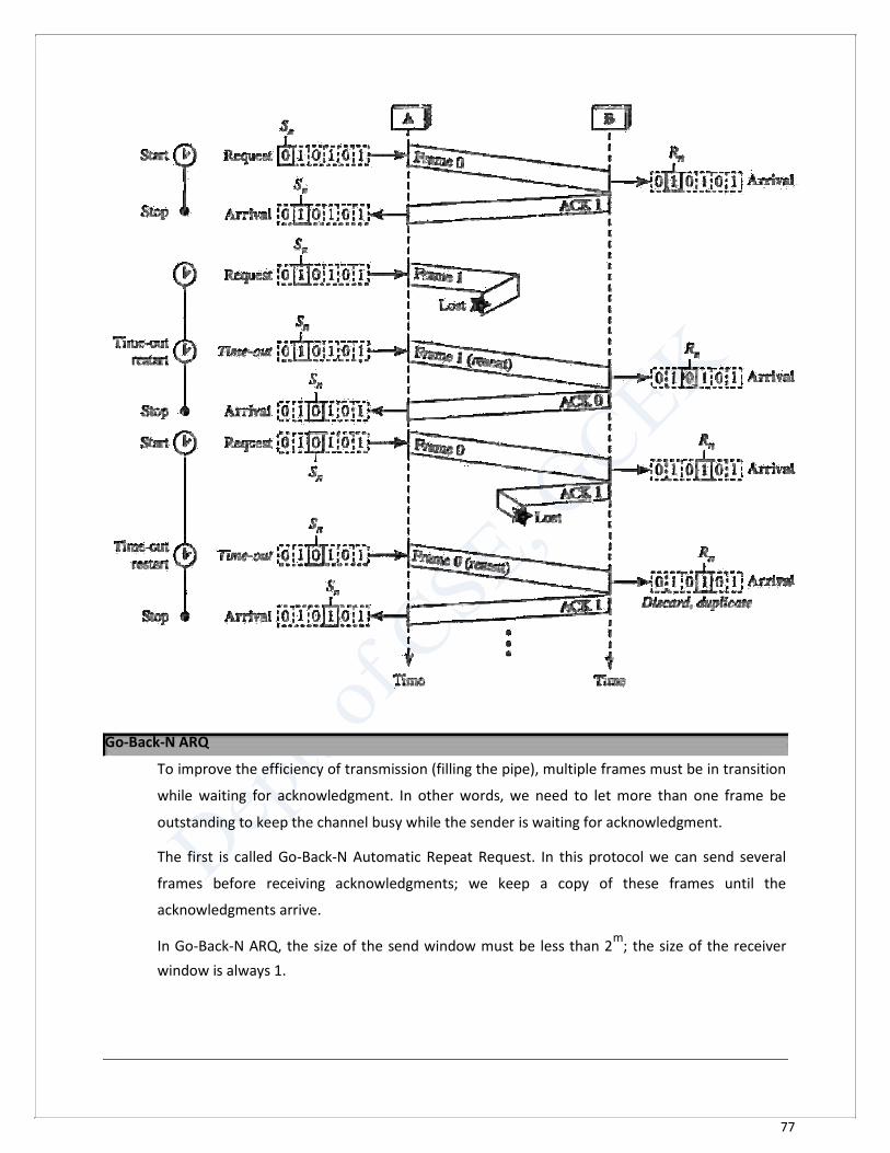
77

Go-Back-N ARQ

To improve the efficiency of transmission (filling the pipe), multiple frames must be in transition

while waiting for acknowledgment. In other words, we need to let more than one frame be

outstanding to keep the channel busy while the sender is waiting for acknowledgment.

The first is called Go-Back-N Automatic Repeat Request. In this protocol we can send several

frames before receiving acknowledgments; we keep a copy of these frames until the

acknowledgments arrive.

In Go-Back-N ARQ, the size of the send window must be less than 2m

; the size of the receiver

window is always 1.

78

Sequence Numbers

Frames from a sending station are numbered sequentially. However, because we need to include the

sequence number of each frame in the header, we need to set a limit. If the header of the frame allows

m bits for the sequence number, the sequence numbers range from 0 to 2m

- 1. For example, if m is 4,

the only sequence numbers are 0 through 15 inclusive. However, we can repeat the sequence. So the

sequence numbers are 0, 1, 2, 3, 4, 5, 6, 7, 8, 9, 10, 11, 12, 13, 14, 15, 0, 1, 2, 3, 4, 5, 6, 7, 8, 9, 10, 11, .......

In other words, the sequence numbers are modulo-2m

. In the Go-Back-N Protocol, the sequence

numbers are modulo 2m

, where m is the size of the sequence number field in bits. . Sliding Window In Go-Back-N Automatic Repeat Request, the sliding window is an abstract concept that defines the

range of sequence numbers that is the concern of the sender and receiver. In other words, the sender

and receiver need to deal with only part of the possible sequence numbers. The range which is the

concern of the sender is called the send sliding window; the range that is the concern of the receiver is

called the receive sliding window. The window at any time divides the possible sequence numbers into four regions.

The first region, from the far left to the left wall of the window, defines the sequence numbers

belonging to frames that are already acknowledged. The sender does not worry about these

frames and keeps no copies of them.

The second region defines the range of sequence numbers belonging to the frames that are sent

and have an unknown status. The sender needs to wait to find out if these frames have been

received or were lost. We call these outstanding frames.

The third range defines the range of sequence numbers for frames that can be sent; however,

the corresponding data packets have not yet been received from the network layer.

Finally, the fourth region defines sequence numbers that cannot be used until the window

slides.

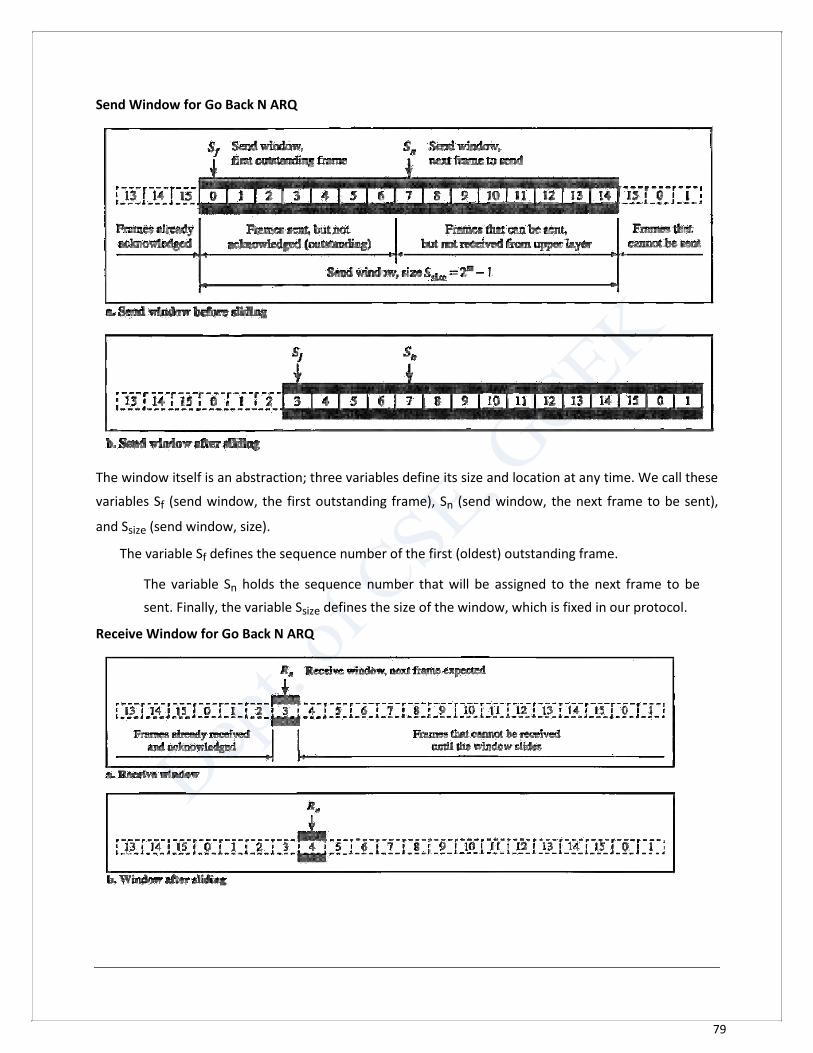
79

Send Window for Go Back N ARQ

The window itself is an abstraction; three variables define its size and location at any time. We call these

variables Sf (send window, the first outstanding frame), Sn (send window, the next frame to be sent),

and Ssize (send window, size).

The variable Sf defines the sequence number of the first (oldest) outstanding frame.

The variable Sn holds the sequence number that will be assigned to the next frame to be

sent. Finally, the variable Ssize defines the size of the window, which is fixed in our protocol. Receive Window for Go Back N ARQ

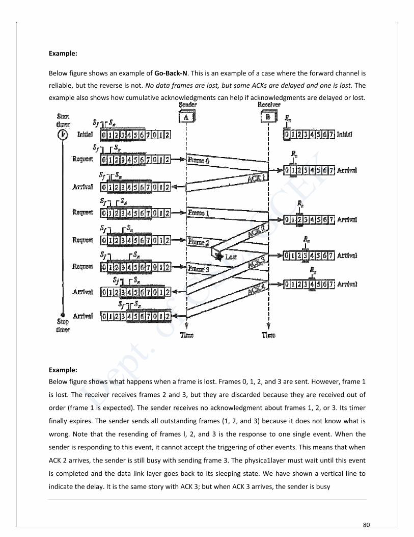
80

Example: Below figure shows an example of Go-Back-N. This is an example of a case where the forward channel is

reliable, but the reverse is not. No data frames are lost, but some ACKs are delayed and one is lost. The

example also shows how cumulative acknowledgments can help if acknowledgments are delayed or lost.

Example: Below figure shows what happens when a frame is lost. Frames 0, 1, 2, and 3 are sent. However, frame 1

is lost. The receiver receives frames 2 and 3, but they are discarded because they are received out of

order (frame 1 is expected). The sender receives no acknowledgment about frames 1, 2, or 3. Its timer

finally expires. The sender sends all outstanding frames (1, 2, and 3) because it does not know what is

wrong. Note that the resending of frames l, 2, and 3 is the response to one single event. When the

sender is responding to this event, it cannot accept the triggering of other events. This means that when

ACK 2 arrives, the sender is still busy with sending frame 3. The physica1layer must wait until this event

is completed and the data link layer goes back to its sleeping state. We have shown a vertical line to

indicate the delay. It is the same story with ACK 3; but when ACK 3 arrives, the sender is busy

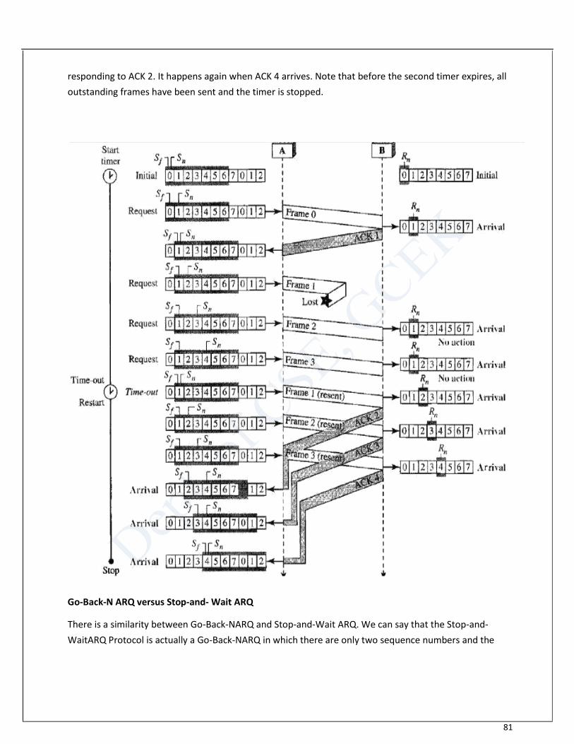
81

responding to ACK 2. It happens again when ACK 4 arrives. Note that before the second timer expires, all

outstanding frames have been sent and the timer is stopped.

Go-Back-N ARQ versus Stop-and- Wait ARQ There is a similarity between Go-Back-NARQ and Stop-and-Wait ARQ. We can say that the Stop-and-

WaitARQ Protocol is actually a Go-Back-NARQ in which there are only two sequence numbers and the

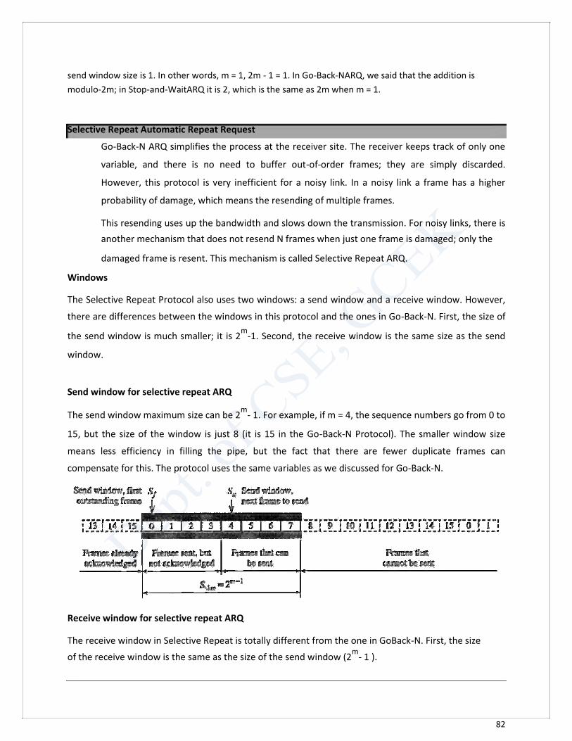
82

send window size is 1. In other words, m = 1, 2m - 1 = 1. In Go-Back-NARQ, we said that the addition is

modulo-2m; in Stop-and-WaitARQ it is 2, which is the same as 2m when m = 1.

Selective Repeat Automatic Repeat Request

Go-Back-N ARQ simplifies the process at the receiver site. The receiver keeps track of only one

variable, and there is no need to buffer out-of-order frames; they are simply discarded.

However, this protocol is very inefficient for a noisy link. In a noisy link a frame has a higher

probability of damage, which means the resending of multiple frames.

This resending uses up the bandwidth and slows down the transmission. For noisy links, there is

another mechanism that does not resend N frames when just one frame is damaged; only the

damaged frame is resent. This mechanism is called Selective Repeat ARQ. Windows The Selective Repeat Protocol also uses two windows: a send window and a receive window. However,

there are differences between the windows in this protocol and the ones in Go-Back-N. First, the size of

the send window is much smaller; it is 2m

-1. Second, the receive window is the same size as the send

window.

Send window for selective repeat ARQ

The send window maximum size can be 2m

- 1. For example, if m = 4, the sequence numbers go from 0 to

15, but the size of the window is just 8 (it is 15 in the Go-Back-N Protocol). The smaller window size

means less efficiency in filling the pipe, but the fact that there are fewer duplicate frames can

compensate for this. The protocol uses the same variables as we discussed for Go-Back-N.

Receive window for selective repeat ARQ The receive window in Selective Repeat is totally different from the one in GoBack-N. First, the size

of the receive window is the same as the size of the send window (2m

- 1 ).

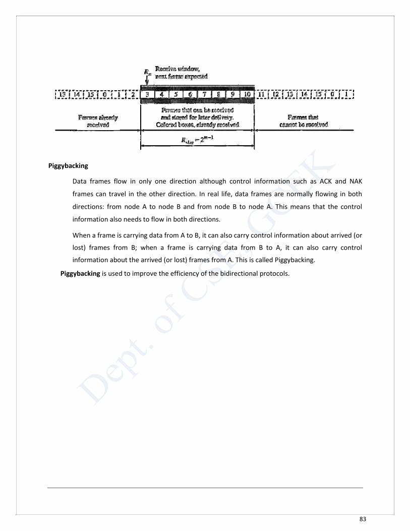
83

Piggybacking

Data frames flow in only one direction although control information such as ACK and NAK

frames can travel in the other direction. In real life, data frames are normally flowing in both

directions: from node A to node B and from node B to node A. This means that the control

information also needs to flow in both directions.

When a frame is carrying data from A to B, it can also carry control information about arrived (or

lost) frames from B; when a frame is carrying data from B to A, it can also carry control

information about the arrived (or lost) frames from A. This is called Piggybacking.

Piggybacking is used to improve the efficiency of the bidirectional protocols.

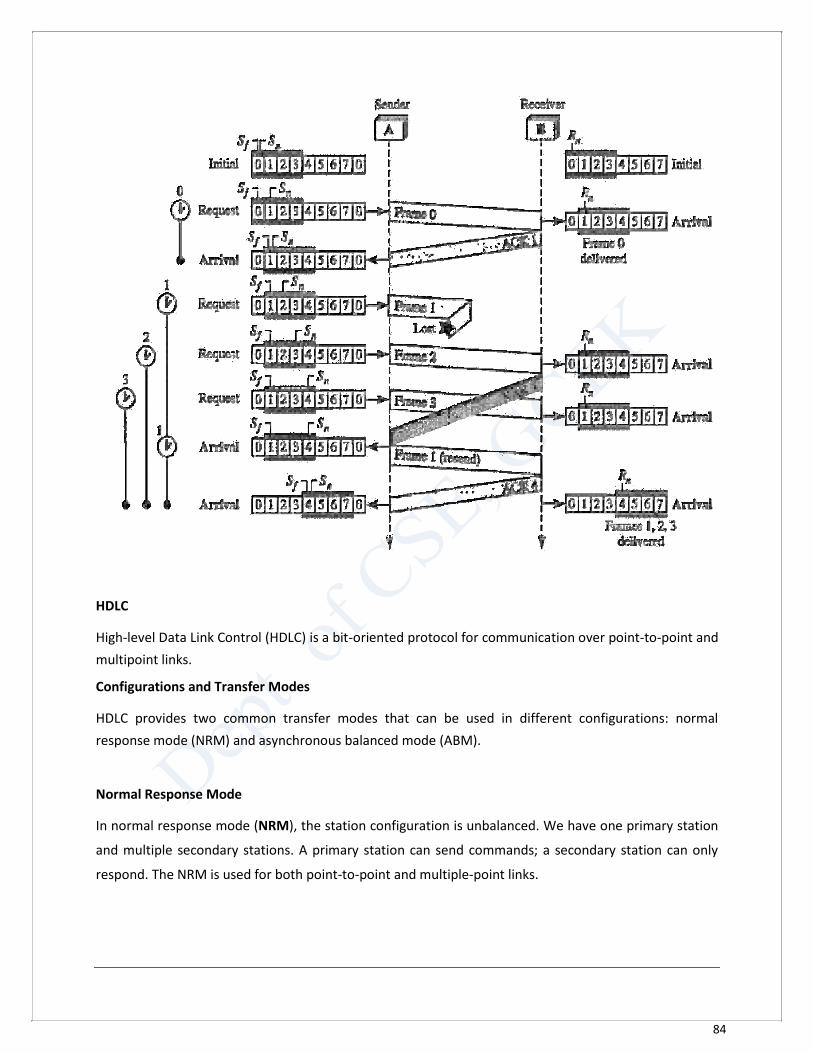
84

HDLC High-level Data Link Control (HDLC) is a bit-oriented protocol for communication over point-to-point and

multipoint links. Configurations and Transfer Modes HDLC provides two common transfer modes that can be used in different configurations: normal

response mode (NRM) and asynchronous balanced mode (ABM).

Normal Response Mode In normal response mode (NRM), the station configuration is unbalanced. We have one primary station

and multiple secondary stations. A primary station can send commands; a secondary station can only

respond. The NRM is used for both point-to-point and multiple-point links.

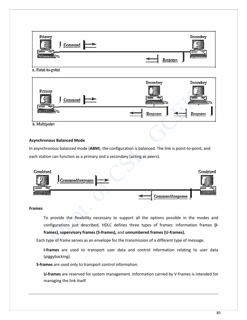
85

Asynchronous Balanced Mode In asynchronous balanced mode (ABM), the configuration is balanced. The link is point-to-point, and each station can function as a primary and a secondary (acting as peers).

Frames

To provide the flexibility necessary to support all the options possible in the modes and

configurations just described, HDLC defines three types of frames: information frames (I-

frames), supervisory frames (S-frames), and unnumbered frames (U-frames).

Each type of frame serves as an envelope for the transmission of a different type of message.

I-frames are used to transport user data and control information relating to user data

(piggybacking).

S-frames are used only to transport control information.

U-frames are reserved for system management. Information carried by V-frames is intended for

managing the link itself.

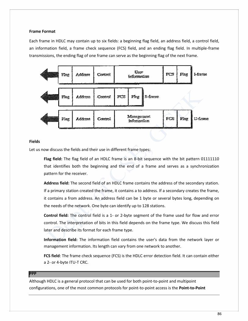
86

Frame Format Each frame in HDLC may contain up to six fields: a beginning flag field, an address field, a control field,

an information field, a frame check sequence (FCS) field, and an ending flag field. In multiple-frame

transmissions, the ending flag of one frame can serve as the beginning flag of the next frame.

Fields Let us now discuss the fields and their use in different frame types:

Flag field: The flag field of an HDLC frame is an 8-bit sequence with the bit pattern 01111110

that identifies both the beginning and the end of a frame and serves as a synchronization

pattern for the receiver.

Address field: The second field of an HDLC frame contains the address of the secondary station.

If a primary station created the frame, it contains a to address. If a secondary creates the frame,

it contains a from address. An address field can be 1 byte or several bytes long, depending on

the needs of the network. One byte can identify up to 128 stations.

Control field: The control field is a 1- or 2-byte segment of the frame used for flow and error

control. The interpretation of bits in this field depends on the frame type. We discuss this field

later and describe its format for each frame type.

Information field: The information field contains the user's data from the network layer or

management information. Its length can vary from one network to another.

FCS field: The frame check sequence (FCS) is the HDLC error detection field. It can contain either

a 2- or 4-byte ITU-T CRC.

PPP Although HDLC is a general protocol that can be used for both point-to-point and multipoint

configurations, one of the most common protocols for point-to-point access is the Point-to-Point

87

Protocol (PPP). Today, millions of Internet users who need to connect their home computers to the

server of an Internet service provider use PPP.

PPP provides several services:

1. PPP defines the format of the frame to be exchanged between devices.

2. PPP defines how two devices can negotiate the establishment of the link and the exchange of data.

3. PPP defines how network layer data are encapsulated in the data link frame.

4. PPP defines how two devices can authenticate each other.

5. PPP provides multiple network layer services supporting a variety of network layer protocols.

6. PPP provides connections over multiple links.

7. PPP provides network address configuration. This is particularly useful when a home user needs a temporary

network address to connect to the Internet.

On the other hand, to keep PPP simple, several services are missing:

I. PPP does not provide flow control. A sender can send several frames one after another with no

concern about overwhelming the receiver.

2. PPP has a very simple mechanism for error control. A CRC field is used to detect errors. If the frame is corrupted,

it is silently discarded; the upper-layer protocol needs to take care of the problem. Lack of error control and

sequence numbering may cause a packet to be received out of order.

3. PPP does not provide a sophisticated addressing mechanism to handle frames in a multipoint configuration. Frame Format of PPP Flag: A PPP frame starts and ends with a I-byte flag with the bit pattern 01111110. Although this pattern

is the same as that used in HDLC, there is a big difference. PPP is a byte-oriented protocol; HDLC is a bit-

oriented protocol.

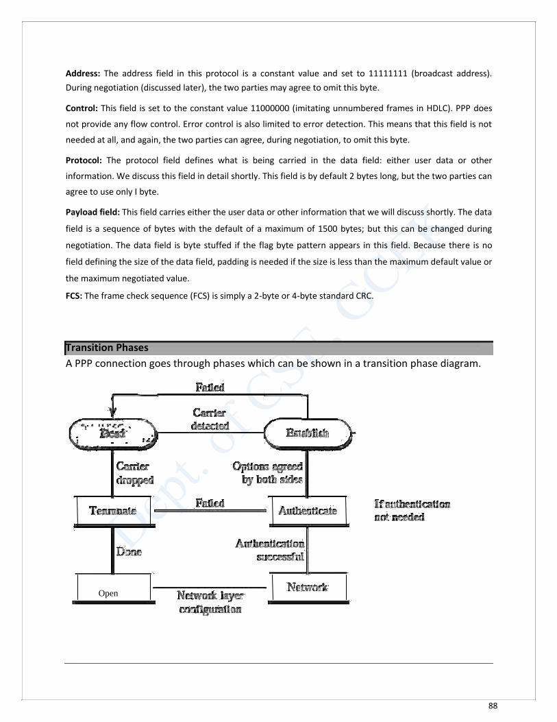
88

Address: The address field in this protocol is a constant value and set to 11111111 (broadcast address).

During negotiation (discussed later), the two parties may agree to omit this byte. Control: This field is set to the constant value 11000000 (imitating unnumbered frames in HDLC). PPP does

not provide any flow control. Error control is also limited to error detection. This means that this field is not

needed at all, and again, the two parties can agree, during negotiation, to omit this byte. Protocol: The protocol field defines what is being carried in the data field: either user data or other

information. We discuss this field in detail shortly. This field is by default 2 bytes long, but the two parties can

agree to use only I byte. Payload field: This field carries either the user data or other information that we will discuss shortly. The data

field is a sequence of bytes with the default of a maximum of 1500 bytes; but this can be changed during

negotiation. The data field is byte stuffed if the flag byte pattern appears in this field. Because there is no

field defining the size of the data field, padding is needed if the size is less than the maximum default value or

the maximum negotiated value. FCS: The frame check sequence (FCS) is simply a 2-byte or 4-byte standard CRC.

Transition Phases A PPP connection goes through phases which can be shown in a transition phase diagram. i

Open

89

Dead: In the dead phase the link is not being used. There is no active carrier (at the physical layer) and

the line is quiet. Establish: When one of the nodes starts the communication, the connection goes into this phase. In this

phase, options are negotiated between the two parties. If the negotiation is successful, the system goes

to the authentication phase (if authentication is required) or directly to the networking phase. The link

control protocol packets, discussed shortly, are used for this purpose. Several packets may be

exchanged here. Authenticate: The authentication phase is optional; the two nodes may decide, during the

establishment phase, not to skip this phase. However, if they decide to proceed with authentication,

they send several authentication packets, discussed later. If the result is successful, the connection goes

to the networking phase; otherwise, it goes to the termination phase. Network: In the network phase, negotiation for the network layer protocols takes place. PPP specifies

that two nodes establish a network layer agreement before data at the network layer can be exchanged.

The reason is that PPP supports multiple protocols at the network layer. If a node is running multiple

protocols simultaneously at the network layer, the receiving node needs to know which protocol will

receive the data. Open: In the open phase, data transfer takes place. When a connection reaches this phase, the

exchange of data packets can be started. The connection remains in this phase until one of the

endpoints wants to terminate the connection. Terminate: In the termination phase the connection is terminated. Several packets are exchanged

between the two ends for house cleaning and closing the link.

90

This page is left vacant intentionally