The Pennsylvania State University

The Graduate School

Department of Computer Science and Engineering

DATA COLLECTION USING RFID AND MOBILE READERS

A Thesis in

Computer Science and Engineering

by

Michael Lin

c© 2008 Michael Lin

Submitted in Partial Fulfillmentof the Requirements

for the Degree of

Master of Science

May 2008

The thesis of Michael Lin was reviewed and approved* by the following.

Thomas F. La PortaDistinguished Professor of Computer Science and EngineeringThesis Adviser

Guohong CaoAssociate Professor of Computer Science and Engineering

Raj AcharyaProfessor of Computer Science and EngineeringHead of the Department of Computer Science and Engineering

*Signatures are on file in the Graduate School.

iii

Abstract

RFID tags are widely used to track inventory as it enters and exits warehouses. However,

the limitations of passive RFID technology prevents its use in real-time inventory management.

In this thesis, we present two novel methods of combining RFID technology with mobile robots

to extend RFID’s use in real-time inventory management. Our first method uses both a mesh

network of active RFID tags and a single mobile reader to enable real-time querying of goods

in a warehouse. The combination of the mesh network and mobile reader gives the system

the flexibility to find data paths that efficiently distribute energy consumption, reducing power

consumption by up to 80% while maintaining query response times of under 40 seconds. We also

present a system of multiple mobile readers connected via a base station or ad-hoc network in a

passive RFID tag-equipped warehouse. We find that our flexible grid robot movement algorithm

performed within 5% of the optimal naive algorithm in the base station case, and outperformed

all other algorithms by up to 80% in the ad-hoc case. We conclude that using both RFID

and mobile readers provides a superb combination of capabilities supporting real-time inventory

management.

iv

Table of Contents

List of Tables . . . . . . . . . . . . . . . . . . . . . . . . . . . . . . . . . . . . . . . . . . . vi

List of Figures . . . . . . . . . . . . . . . . . . . . . . . . . . . . . . . . . . . . . . . . . . vii

Chapter 1. Introduction . . . . . . . . . . . . . . . . . . . . . . . . . . . . . . . . . . . . . 11.1 RFID Tags . . . . . . . . . . . . . . . . . . . . . . . . . . . . . . . . . . . . . 21.2 Mobile Readers . . . . . . . . . . . . . . . . . . . . . . . . . . . . . . . . . . . 4

Chapter 2. Single Reader Data Gathering in Active RFID Networks . . . . . . . . . . . . 62.1 Backbone Setup . . . . . . . . . . . . . . . . . . . . . . . . . . . . . . . . . . . 7

2.1.1 Index Node Selection . . . . . . . . . . . . . . . . . . . . . . . . . . . . 72.1.2 Energy Requirements . . . . . . . . . . . . . . . . . . . . . . . . . . . 102.1.3 Example . . . . . . . . . . . . . . . . . . . . . . . . . . . . . . . . . . . 112.1.4 Indexing . . . . . . . . . . . . . . . . . . . . . . . . . . . . . . . . . . . 12

2.2 Backbone Network Formation . . . . . . . . . . . . . . . . . . . . . . . . . . . 132.2.1 Backbone Network Formation Algorithm . . . . . . . . . . . . . . . . . 132.2.2 Updating the Backbone Network . . . . . . . . . . . . . . . . . . . . . 17

2.3 Query Resolution . . . . . . . . . . . . . . . . . . . . . . . . . . . . . . . . . . 172.3.1 Query Types . . . . . . . . . . . . . . . . . . . . . . . . . . . . . . . . 172.3.2 Query Time Constraints . . . . . . . . . . . . . . . . . . . . . . . . . . 182.3.3 Resolving Simple Queries . . . . . . . . . . . . . . . . . . . . . . . . . 19

2.3.3.1 Determining the Query Resolution Time . . . . . . . . . . . 202.3.3.2 Protocol Outline . . . . . . . . . . . . . . . . . . . . . . . . . 22

2.3.4 Resolving Complex Queries . . . . . . . . . . . . . . . . . . . . . . . . 222.4 Implementation and Simulation . . . . . . . . . . . . . . . . . . . . . . . . . . 232.5 Results . . . . . . . . . . . . . . . . . . . . . . . . . . . . . . . . . . . . . . . . 242.6 Conclusion . . . . . . . . . . . . . . . . . . . . . . . . . . . . . . . . . . . . . . 25

Chapter 3. Multiple Reader Data Gathering with Passive RFID Tags . . . . . . . . . . . 313.1 Mathematical Model . . . . . . . . . . . . . . . . . . . . . . . . . . . . . . . . 32

3.1.1 Expected Number of Hops in an Active Tag Network . . . . . . . . . . 333.1.2 Expected Number of Transmissions in an Active Tag Network . . . . . 333.1.3 Expected Lifetime of Active Tag Network . . . . . . . . . . . . . . . . 343.1.4 Cost Analysis for Active Tag Network . . . . . . . . . . . . . . . . . . 343.1.5 Cost Analysis for Passive Tag Network . . . . . . . . . . . . . . . . . . 35

3.2 Algorithms for Fully Connected Multiple Readers . . . . . . . . . . . . . . . . 353.2.1 Locating Data Sources . . . . . . . . . . . . . . . . . . . . . . . . . . . 353.2.2 Data Collection . . . . . . . . . . . . . . . . . . . . . . . . . . . . . . . 36

3.2.2.1 Areas of Responsibility . . . . . . . . . . . . . . . . . . . . . 363.2.2.2 Rest Points . . . . . . . . . . . . . . . . . . . . . . . . . . . . 37

3.2.3 Fully Connected Protocol . . . . . . . . . . . . . . . . . . . . . . . . . 383.2.4 Fully Connected Protocol Variations . . . . . . . . . . . . . . . . . . . 39

3.3 Algorithms for Multi-hop Connected Multiple Readers . . . . . . . . . . . . . 403.3.1 Multi-hop Protocol . . . . . . . . . . . . . . . . . . . . . . . . . . . . . 423.3.2 Multi-hop Protocol Variations . . . . . . . . . . . . . . . . . . . . . . . 43

3.4 Implementation and Simulation . . . . . . . . . . . . . . . . . . . . . . . . . . 43

v

3.4.1 Simulation Details . . . . . . . . . . . . . . . . . . . . . . . . . . . . . 443.4.1.1 Queries . . . . . . . . . . . . . . . . . . . . . . . . . . . . . . 44

3.5 Results . . . . . . . . . . . . . . . . . . . . . . . . . . . . . . . . . . . . . . . . 463.5.1 Fully Connected Results . . . . . . . . . . . . . . . . . . . . . . . . . . 463.5.2 Multi-hop Results . . . . . . . . . . . . . . . . . . . . . . . . . . . . . 47

3.6 Analysis . . . . . . . . . . . . . . . . . . . . . . . . . . . . . . . . . . . . . . . 483.6.1 Secondary Distance . . . . . . . . . . . . . . . . . . . . . . . . . . . . . 483.6.2 Results Analysis . . . . . . . . . . . . . . . . . . . . . . . . . . . . . . 49

3.7 Conclusion . . . . . . . . . . . . . . . . . . . . . . . . . . . . . . . . . . . . . . 51

Chapter 4. Conclusion . . . . . . . . . . . . . . . . . . . . . . . . . . . . . . . . . . . . . . 63

References . . . . . . . . . . . . . . . . . . . . . . . . . . . . . . . . . . . . . . . . . . . . . 65

vi

List of Tables

2.1 Notation . . . . . . . . . . . . . . . . . . . . . . . . . . . . . . . . . . . . . . . . . 72.2 Index Node Selection Messages . . . . . . . . . . . . . . . . . . . . . . . . . . . . 102.3 Indexing Messages . . . . . . . . . . . . . . . . . . . . . . . . . . . . . . . . . . . 132.4 Backbone Network Messages . . . . . . . . . . . . . . . . . . . . . . . . . . . . . 17

3.1 Simulation parameters. . . . . . . . . . . . . . . . . . . . . . . . . . . . . . . . . . 443.2 Aggregate results from skew and no skew simulations with 16 mobile readers

moving at 3 feet per second. . . . . . . . . . . . . . . . . . . . . . . . . . . . . . . 50

vii

List of Figures

2.1 Index Selection Example . . . . . . . . . . . . . . . . . . . . . . . . . . . . . . . . 112.2 Node identity dissemination . . . . . . . . . . . . . . . . . . . . . . . . . . . . . . 142.3 Ring formation example . . . . . . . . . . . . . . . . . . . . . . . . . . . . . . . . 162.4 Hybrid and movement-only success rate . . . . . . . . . . . . . . . . . . . . . . . 272.5 Total distance travelled . . . . . . . . . . . . . . . . . . . . . . . . . . . . . . . . 282.6 Movement of the mobile reader in the hybrid and pure movement schemes. . . . 292.7 Power consumption per node . . . . . . . . . . . . . . . . . . . . . . . . . . . . . 30

3.1 Query forwarding in multi-hop operation . . . . . . . . . . . . . . . . . . . . . . . 523.2 Average time per query v. mobile reader speed with four fully connected readers 533.3 Average time per query v. mobile reader speed with 16 fully connected readers . 543.4 Distance v. mobile reader speed with four fully connected readers . . . . . . . . . 553.5 Distance v. mobile reader speed with 16 fully connected readers . . . . . . . . . . 563.6 Time v. mobile reader speed with 16 multi-hop connected readers . . . . . . . . 573.7 Distance v. mobile reader speed with 16 multi-hop connected readers . . . . . . . 583.8 Secondary distance v. mobile reader speed with 16 multi-hop connected readers . 593.9 Secondary distance example . . . . . . . . . . . . . . . . . . . . . . . . . . . . . . 603.10 Reader positions using the naive algorithm . . . . . . . . . . . . . . . . . . . . . 613.11 Reader positions using the flexible grid algorithm . . . . . . . . . . . . . . . . . . 62

1

Chapter 1

Introduction

Radio frequency identification (RFID) tags are an ideal foundation for inventory control

systems. They are small, very low-cost, and can store more than enough information to uniquely

identify items in even the largest warehouses. However, RFID tags’ simplicity also limits their

functionality. Although they can store information, typical passive RFID tags cannot perform

calculations or actively broadcast data. Furthermore, passive RFID tags must be read from

within roughly 10 feet, making it impossible to install an RFID reader that covers an entire

warehouse.

These limitations mean that although RFID can be used to track inventory on a high

level, such as determining which warehouse an item is in, it cannot be used to determine the

exact location of the item. Current inventory control systems using RFID read items’ RFID

tags when the item enters and leaves the warehouse, but once the item is in the warehouse

the RFID tag remains unused. This system of reading RFID tags prevents real-time inventory

access. Furthermore, since items are only read when they are brought into the warehouse, their

exact current location in the warehouse cannot be known. This is especially problematic in large

warehouses, where items can often be misplaced and difficult to relocate.

Current RFID technology is also of limited use in temporary warehouses. For example, a

military may quickly set up a temporary supply depot while preparing for a battle. In a chaotic

temporary warehouse, accurate inventory control is difficult to achieve and highly valuable. How-

ever, these temporary warehouses may not have the necessary infrastructure to support current

RFID inventory control systems, preventing their use. Temporary warehouses require that an

2

inventory control system be robust enough to cope with unannounced item arrival and departure,

as well as being simple enough to be deployed in an area with poor infrastructure support.

In this thesis we present two novel methods of using RFID to extend the capabilities of

inventory control systems to include real-time inventory control and infrastructure-free inventory

control. The first method we propose takes advantage of a new type of RFID tag known as an

active RFID tag, also known as simply active tags. Active tags are similar to passive RFID tags,

but are powered and able to perform computations and communicate with other tags or readers.

We supplement our use of active tags with a mobile robot with an active tag reader, referred to

as a mobile reader. We capitalize on the strengths of both active tags and the mobile reader to

provide a robust real-time inventory system.

The second method we propose in this thesis further explores the development of the

mobile reader while eliminating the requirement for active tags. Since items in warehouses are

often tagged with passive tags already, this greatly reduces the cost of entry for our system. To

compensate for the loss of capabilities from switching from active tags to passive tags, we increase

the number and complexity of the mobile readers.

In the remainder of this chapter, we discuss passive and active RFID in detail and introduce

our mobile readers. The remainder of this thesis is organized as follows: in Chapter 2 we present

a method of using active RFID tags and a single mobile reader to achieve efficient real-time

inventory control. In Chapter 3, we present a method using passive RFID tags and multiple

mobile readers. We conclude in Chapter 4.

1.1 RFID Tags

Currently, there are two major types of RFID tags in use: passive and active. Passive

tags are widespread, while active tags have only recently been introduced. Passive RFID tags

are simple, unpowered circuits that can only be read by a powered reader. Since passive tags

can only hold a few kilobytes of information, they are commonly used as identifiers for items

3

ranging from inventory in warehouses to patients in hospitals. They can perform no calculations

or transmissions; they can only be read. Some passive tags can be rewritten while being read,

while others simply hold a unique identifier and cannot be changed. Although long-range reading

of passive RFID tags is possible in some cases, most uses of passive tags assume readers will be

within three feet of tags they are reading. Although passive tags have very limited capabilities,

their simplicity allows them to be mass-produced at a very low cost. Passive tags can be printed

in rolls of thousands for only a few cents per tag. Additionally, since passive tags are unpowered,

their lifetimes are essentially unlimited, barring destruction of the tag itself.

Unlike passive tags, active tags are powered and can perform basic processing. Active tags

can hold far more information than passive tags, in the range of hundreds of kilobytes, rather

than tens. Furthermore, they can transmit over an antenna, which allows them to be read much

more easily than passive tags, and in some cases allows them to communicate with each other.

Naturally, this complexity comes at a cost. Since active tags are powered, their lifetimes are

limited to the lifetimes of their batteries. Furthermore, individual active tags are an order of

magnitude more expensive than passive tags: typical active tags are priced in the tens of dollars,

compared to the tens of cents of passive tags. Active tags find use in similar situations as passive

tags, although their high cost limits them from being as ubiquitous as passive tags. Whereas

each item in a warehouse may be tagged with a passive tag, active tags are commonly built into

pallets or other storage containers, with an expected lifetime of five years.

The additional capabilities of active tags allow them to be used in much more complex

ways than passive tags. Their capabilities essentially mirror those of sensor motes, such as the

Crossbow MicaZ [1], which allows the large body of research developed for sensors and sensor

networks to be used to design active tag systems. In particular, much research has been done on

ad-hoc networks formed between large numbers of sensor motes, also known as mesh networks.

We leverage this existing research in mesh networks using sensors to develop mesh networks using

active tags.

4

Mesh networks’ essential functions are the same as traditional networks, but the limitations

of wireless technology and the limited resources of the motes change the dynamics of the network.

Most importantly, mesh networks are completely decentralized, which combined with the limited

resources of the nodes makes routing very difficult. Existing research has provided a number of

solutions to the routing problem, which we take of advantage of in our single reader protocol.

Although active tags provide new capabilities that allow for more robust system design,

they are still limited by battery life concerns. Battery life is critical in actual warehouse op-

erations, since there will typically be hundreds or thousands of active tags in a warehouse. It

is simply infeasible to replace batteries on such a large scale, so active tags are designed to be

disposable, with an expected battery life of up to five years. Network transmission is the most

power consuming operation an active tag can perform, so we must be extremely economical with

transmissions. This is problematic in a data querying system, where query responses can be

very large; for example, a single query could ask for the full inventory of a crate that contains

hundreds of items. We use mobile readers to ameliorate the impact of large data transfers in

active tag networks, and to enable real-time querying in passive tag networks.

1.2 Mobile Readers

We use mobile readers for two separate but related tasks in each of the systems presented

in this paper. In the active tag system we use a mobile reader to reduce the energy cost of large

data transfers by increasing the time cost. Rather than using the mesh network to transfer a

large dataset, the mobile reader will move to the data to pick it up. Since the mobile reader must

physically travel to the data, this takes more time, but it also reduces energy consumption. In

the passive tag system, there is no mesh network, so all tag reads must be done by the mobile

reader.

The concept of a mobile reader originated from the fact that warehouses often have either

autonomous or human-driven vehicles performing various tasks in the warehouse. Robots can

5

be used in certain situations to pick up or drop off goods, or forklifts can be used by humans

to move large amounts of goods. By simply attaching a small computer and an RFID reader to

such vehicles, warehouses can greatly improve their inventorying. Although we use robots in our

solution, RFID readers can also be attached to humans, for example on a belt clip.

As a prototype for our mobile reader, we used a simple two-wheeled robot design. Our

robots were designed and constructed by Tim Bolbrock, who also provided the programming

interface with the robots. Our robots have a maximum speed of less than 1 meter per second,

which is acceptable for a prototype, but not for a full working model. In our simulations we

anticipated robots with speeds of 0.5 to 5 meters per second. For comparison, a forklift in a

warehouse has a top speed of 5-10 miles per hour, or 2.2-4.5 meters per second.

6

Chapter 2

Single Reader Data Gathering in Active RFID Networks

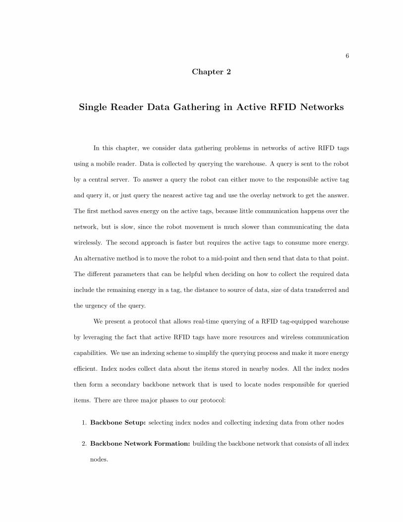
In this chapter, we consider data gathering problems in networks of active RIFD tags

using a mobile reader. Data is collected by querying the warehouse. A query is sent to the robot

by a central server. To answer a query the robot can either move to the responsible active tag

and query it, or just query the nearest active tag and use the overlay network to get the answer.

The first method saves energy on the active tags, because little communication happens over the

network, but is slow, since the robot movement is much slower than communicating the data

wirelessly. The second approach is faster but requires the active tags to consume more energy.

An alternative method is to move the robot to a mid-point and then send that data to that point.

The different parameters that can be helpful when deciding on how to collect the required data

include the remaining energy in a tag, the distance to source of data, size of data transferred and

the urgency of the query.

We present a protocol that allows real-time querying of a RFID tag-equipped warehouse

by leveraging the fact that active RFID tags have more resources and wireless communication

capabilities. We use an indexing scheme to simplify the querying process and make it more energy

efficient. Index nodes collect data about the items stored in nearby nodes. All the index nodes

then form a secondary backbone network that is used to locate nodes responsible for queried

items. There are three major phases to our protocol:

1. Backbone Setup: selecting index nodes and collecting indexing data from other nodes

2. Backbone Network Formation: building the backbone network that consists of all index

nodes.

7

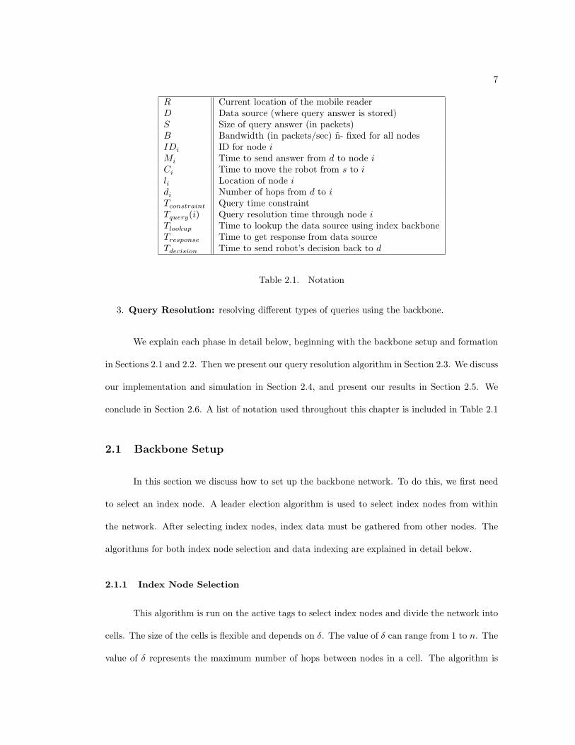
R Current location of the mobile readerD Data source (where query answer is stored)S Size of query answer (in packets)B Bandwidth (in packets/sec) n- fixed for all nodesIDi ID for node iMi Time to send answer from d to node iCi Time to move the robot from s to ili Location of node idi Number of hops from d to iTconstraint Query time constraintTquery(i) Query resolution time through node iTlookup Time to lookup the data source using index backboneTresponse Time to get response from data sourceTdecision Time to send robot’s decision back to d

Table 2.1. Notation

3. Query Resolution: resolving different types of queries using the backbone.

We explain each phase in detail below, beginning with the backbone setup and formation

in Sections 2.1 and 2.2. Then we present our query resolution algorithm in Section 2.3. We discuss

our implementation and simulation in Section 2.4, and present our results in Section 2.5. We

conclude in Section 2.6. A list of notation used throughout this chapter is included in Table 2.1

2.1 Backbone Setup

In this section we discuss how to set up the backbone network. To do this, we first need

to select an index node. A leader election algorithm is used to select index nodes from within

the network. After selecting index nodes, index data must be gathered from other nodes. The

algorithms for both index node selection and data indexing are explained in detail below.

2.1.1 Index Node Selection

This algorithm is run on the active tags to select index nodes and divide the network into

cells. The size of the cells is flexible and depends on δ. The value of δ can range from 1 to n. The

value of δ represents the maximum number of hops between nodes in a cell. The algorithm is

8

based on a leader election algorithm [2], with modifications to optimize for index node selection

rather than leader election. The selection criterion is a function, fi, of available memory, m,

residual energy, e, and distance to the current index node, d. Since we are selecting index nodes,

the amount of available memory and energy determine the usefulness of a node as an index node.

New index nodes will replicate information from old index nodes. Therefore, minimizing the

distance between the new and old index nodes will reduce the overhead of transferring old index

information. Energy consumption will be discussed in more detail below.

Leader election algorithms are based on spanning tree algorithms [3]. The basic concept is

to use directed flooding to create a spanning tree rooted at a single node—the leader. An arbitrary

node begins an election by broadcasting an election message. Nodes that receive this message

participate in the election by forwarding the message to their neighbors. As the tree spreads,

parent-child relationships are established between nodes and the nodes from which they received

the election message. Every node keeps track of its parent and children, as they are important in

the later stages of the algorithm. When every node in the network is participating in the election,

the tree is complete, with nodes on the edge of the network being leaf nodes. The tree then shrinks

back toward the leader along the same paths it took as it grew. To accomplish this, leaf nodes

send an election acknowledgment (not to be confused with the single message acknowledgment

sent upon receipt of the election message) to their parent nodes, who will send their election

acknowledgment to their parent nodes only when they have received election acknowledgments

from all of their children. Eventually all of the election acknowledgments are aggregated as they

go up the tree and arrive at the node that started the election. This node completes the election

by sending a message announcing that it is the leader over the tree that now exists in the network.

In a typical leader election algorithm, an arbitrary node starts the election. However,

since our algorithm has a strictly defined function, fi, for the selection of appropriate leaders, we

can optimize the beginning stages of an election by increasing the likelihood of a highly weighted

node starting an election.

9

We introduce a sliding probability, p, that is proportional to each node’s weight as de-

termined by fi. This probability will then be used to determine whether or not a node will

start an election at each tick of a timer. For example, if we define p as fi

fMAX, a node with

maximal weight will start the election with probability 1. However, if a node’s weight is 50% of

the maximum, it will start an election with probability 0.5 at each tick of the timer. We can

optimize the probability method by choosing a probability function that begins aggressively and

then sharply reduces the probability over time, which increases the number of viable nodes at

the beginning of network formation.

Our algorithm further differs from standard leader election algorithms by selecting multiple

index nodes instead of a single leader node. We want index nodes to be roughly uniformly spread

across the physical area of the network, but an in-network algorithm will generally not have any

information about the physical layout of the network. To overcome this problem, we exploit the

fact that nodes know their location. If two nodes, A and B, come across each other in the course

of the algorithm, A will join the tree of the B if and only if B is less than δ distance away.

With these additions, a leader election will run as follows: a node with a high fi will

start an election with probability pi on each clock tick. When a node starts an election, it

broadcasts a message to its neighbors, which participate in the election by forwarding the message

to their downstream neighbors. This forwarding continues without acknowledgment until a node

times out or all nodes within δ of the originating node are participating in the election. This

determines the cell’s boundaries. Once the boundary has been defined, the edge nodes send an

acknowledgment upstream. Acknowledgments are aggregated and sent to the originating node,

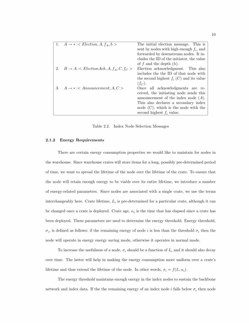
which then sends a message announcing the winner of the election. Table 2.2 summarizes the

messages used in this protocol.

10

1. A → ∗ :< Election, A, fA, h > The initial election message. This issent by nodes with high enough fi, andforwarded by downstream nodes. It in-cludes the ID of the initiator, the valueof f and the depth (h).

2. B → A :< ElectionAck, A, fA, C, fC > Election acknowledgment. This alsoincludes the the ID of that node withthe second highest fi (C) and its value(fC).

3. A → ∗ :< Announcement,A, C > Once all acknowledgments are re-ceived, the initiating node sends thisannouncement of the index node (A).This also declares a secondary indexnode (C), which is the node with thesecond highest fi value.

Table 2.2. Index Node Selection Messages

2.1.2 Energy Requirements

There are certain energy consumption properties we would like to maintain for nodes in

the warehouse. Since warehouse crates will store items for a long, possibly pre-determined period

of time, we want to spread the lifetime of the node over the lifetime of the crate. To ensure that

the node will retain enough energy to be viable over its entire lifetime, we introduce a number

of energy-related parameters. Since nodes are associated with a single crate, we use the terms

interchangeably here. Crate lifetime, Li is pre-determined for a particular crate, although it can

be changed once a crate is deployed. Crate age, αi is the time that has elapsed since a crate has

been deployed. These parameters are used to determine the energy threshold. Energy threshold,

σi, is defined as follows: if the remaining energy of node i is less than the threshold σi then the

node will operate in energy energy saving mode, otherwise it operates in normal mode.

To increase the usefulness of a node, σi should be a function of Li and it should also decay

over time. The latter will help in making the energy consumption more uniform over a crate’s

lifetime and thus extend the lifetime of the node. In other words, σi = f(L,αi).

The energy threshold maintains enough energy in the index nodes to sustain the backbone

network and index data. If the the remaining energy of an index node i falls below σi then node

11

i will notify the secondary index node from the election to have it take over as the new index

node.

2.1.3 Example

B5

D7

A3

C2

1. B5

D7

A3

C2

2.

B5

D7

A3

C2

3. B5

D7

A3

C2

4.

Fig. 2.1. Index Selection Example

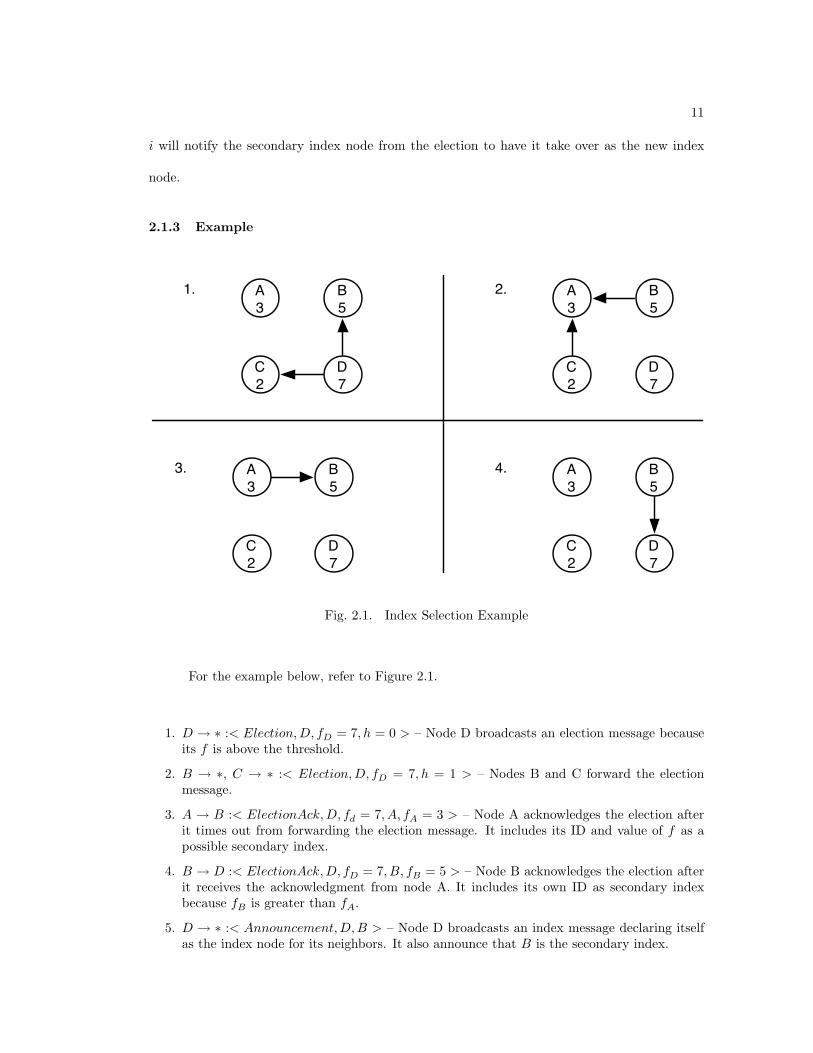
For the example below, refer to Figure 2.1.

1. D → ∗ :< Election, D, fD = 7, h = 0 > – Node D broadcasts an election message becauseits f is above the threshold.

2. B → ∗, C → ∗ :< Election,D, fD = 7, h = 1 > – Nodes B and C forward the electionmessage.

3. A → B :< ElectionAck, D, fd = 7, A, fA = 3 > – Node A acknowledges the election afterit times out from forwarding the election message. It includes its ID and value of f as apossible secondary index.

4. B → D :< ElectionAck, D, fD = 7, B, fB = 5 > – Node B acknowledges the election afterit receives the acknowledgment from node A. It includes its own ID as secondary indexbecause fB is greater than fA.

5. D → ∗ :< Announcement,D,B > – Node D broadcasts an index message declaring itselfas the index node for its neighbors. It also announce that B is the secondary index.

12

2.1.4 Indexing

The basis for our indexing algorithm is ARI, adaptive ring indexing [4]. We use a simplified

version that is less robust but easier to manage. Following the selection of the index nodes, these

nodes will begin the process of collecting index information for the nodes in their cell. The

specific data that nodes will index depends on the items that are in the warehouse. Typical item

properties include color, serial number, type, or category. Since the index node election created

a tree, all nodes belonging to a certain index node have a path to the index node, which greatly

simplifies the process of collecting index data. The index node simply broadcasts a request for

index data to its nearest neighbors, who respond and forward the message to their children in

the tree. Eventually the index node will either finish indexing its cell or refuse to accept more

data due to storage limitations. If the index node’s remaining memory reaches capacity before

it has index data for all of its children, the cell must be split into two. Since this algorithm also

chooses a backup index node, the current index node simply sends a message telling that index

node to split off and form another cell.

After the index node indexes the nodes in its cell for the first time, periodic updates are

necessary to ensure that index data is fresh. Since nodes will not be continually updating, nodes

simply send an update message to their index node whenever their index data changes. While

this minimizes the number of messages sent and ensures that index data will be up-to-date, it

allows the possibility of an index node not knowing when a node has left its cell. An alternative

method for updating is for nodes to send periodic refresh messages, which can include update

information and also ensure that the index node is immediately notified if a node leaves the cell.

The drawback of this method is the high number of messages that will be sent over the lifetime

of the network. If the contents of crates are rarely updated, this can lead to a large number of

redundant messages. The preferred method depends on external properties, such as the pattern

of item removal in the warehouse. Table 2.3 summarizes the messages used in this protocol.

13

1. AI → B :< SendIndex,AI > Index node AI asks all nodes B in the cell to generateindex information

2. B → AI :< IndexData, B > Node B sends index information to AI

Table 2.3. Indexing Messages

2.2 Backbone Network Formation

A backbone network is formed within the mesh network to optimize query resolution.

The algorithm for forming the network and an example are given below. This algorithm is run

during the network bootstrap process and changes to the backbone network are dealt with on an

individual basis.

2.2.1 Backbone Network Formation Algorithm

As stated above, we assume the network uses a geographically-aware routing protocol for

routing between all network nodes. In addition to this network, we form a backbone network of

index nodes that will provide a direct link to index information for query resolution. By using

a backbone network instead of flooding, we can minimize the number of messages needed to

complete a query, thus helping reduce overall energy consumption of the network. The tradeoff

is that energy consumption will be concentrated in index nodes and nodes that connect index

nodes to each other. Index nodes will have high energy consumption regardless of their use in a

backbone network, and the use of an energy aware routing protocol can spread the energy load

on interconnecting nodes.

The backbone network can be considered as a normal network, with non-index nodes

acting as links between index nodes. Thus, normal routing protocols can be used to form the

network, although energy-aware routing should be used to maximize the lifetime of the network.

We use a ring as the topology of the backbone network. The main advantage of using a ring is

its very simple maintenance; each node need only to know its successor and predecessor for the

ring to be complete. If an index node is leaving the ring, due to low energy level, it only needs

14

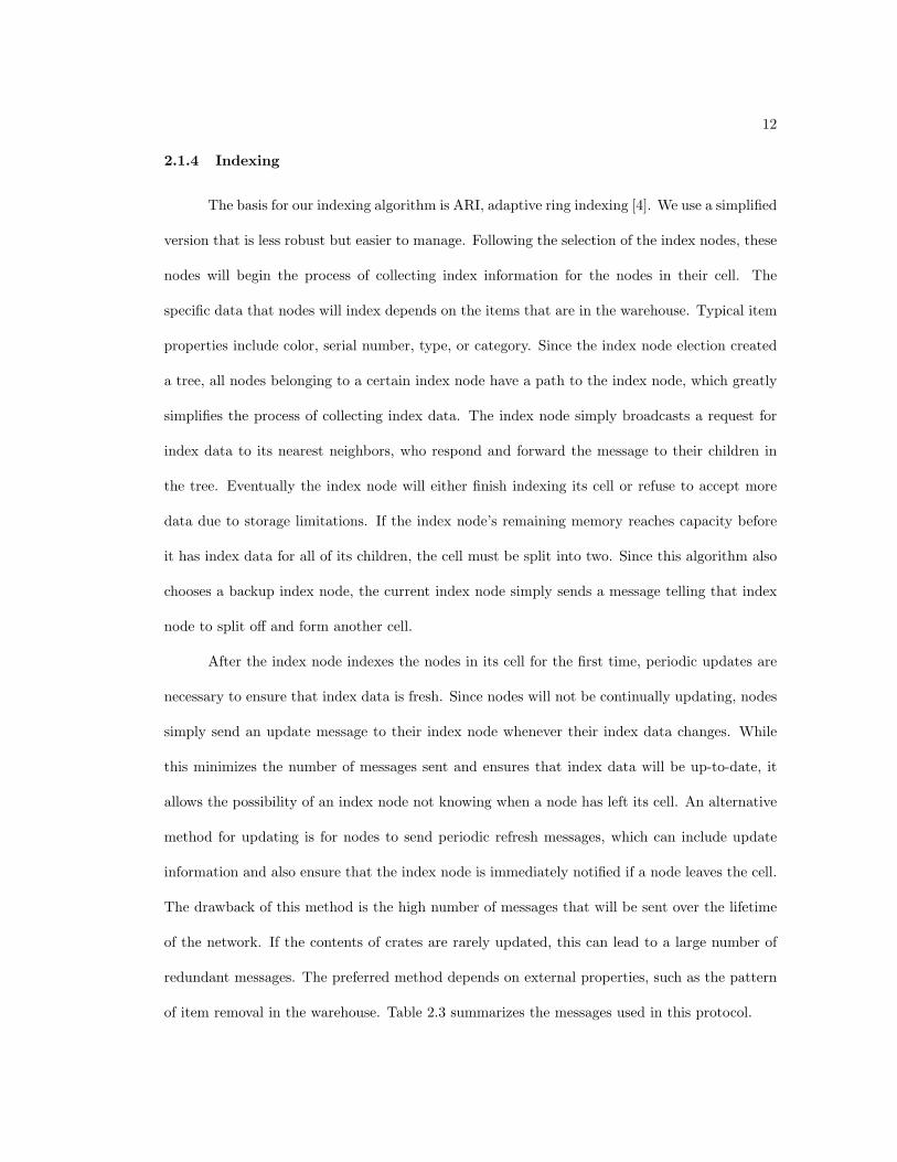
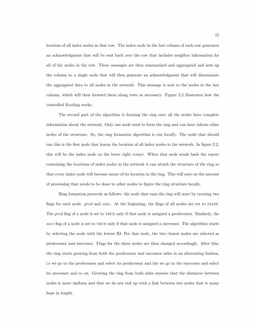
Fig. 2.2. In this example, nodes send identity messages to the right, as shown by the solidarrows. These messages are aggregated and sent down, indicated by the bold arrow. Once thecorner node receives these aggregate messages, they are sent back up and across the warehouse,as shown by the dotted arrows.

to inform these to nodes of the identity of its replacement. We are currently considering other

topologies like a tree which might provide better lookup performance.

The algorithm to form the ring consists of two parts. In the first part, index nodes inform

each other of their location. Next, each index node runs a ring formation algorithm and since all

nodes share the same information about the index locations they will end up forming the same

ring. It is important to note that the ring that is built is virtual and consists of index nodes only.

Because index nodes may be multiple hops away from each other, other nodes in the network

must act as bridges between them. So, even though two nodes may be adjacent in the backbone

ring they might actually be multiple hops away from each other.

To disseminate location information we use a controlled flooding scheme that minimizes

the number of exchanged messages. We use a virtual grid in which index nodes first send discovery

messages down the rows until the edge column is reached. The discovery message accumulates the

15

location of all index nodes in that row. The index node in the last column of each row generates

an acknowledgment that will be sent back over the row that includes neighbor information for

all of the nodes in the row. These messages are then summarized and aggregated and sent up

the column to a single node that will then generate an acknowledgment that will disseminate

the aggregated data to all nodes in the network. This message is sent to the nodes in the last

column, which will then forward them along rows as necessary. Figure 2.2 illustrates how the

controlled flooding works.

The second part of the algorithm is forming the ring once all the nodes have complete

information about the network. Only one node need to form the ring and can later inform other

nodes of the structure. So, the ring formation algorithm is run locally. The node that should

run this is the first node that learns the location of all index nodes in the network. In figure 2.2,

this will be the index node on the lower right corner. When that node sends back the report

containing the locations of index nodes in the network it can attach the structure of the ring so

that every index node will become aware of its location in the ring. This will save on the amount

of processing that needs to be done in other nodes to figure the ring structure locally.

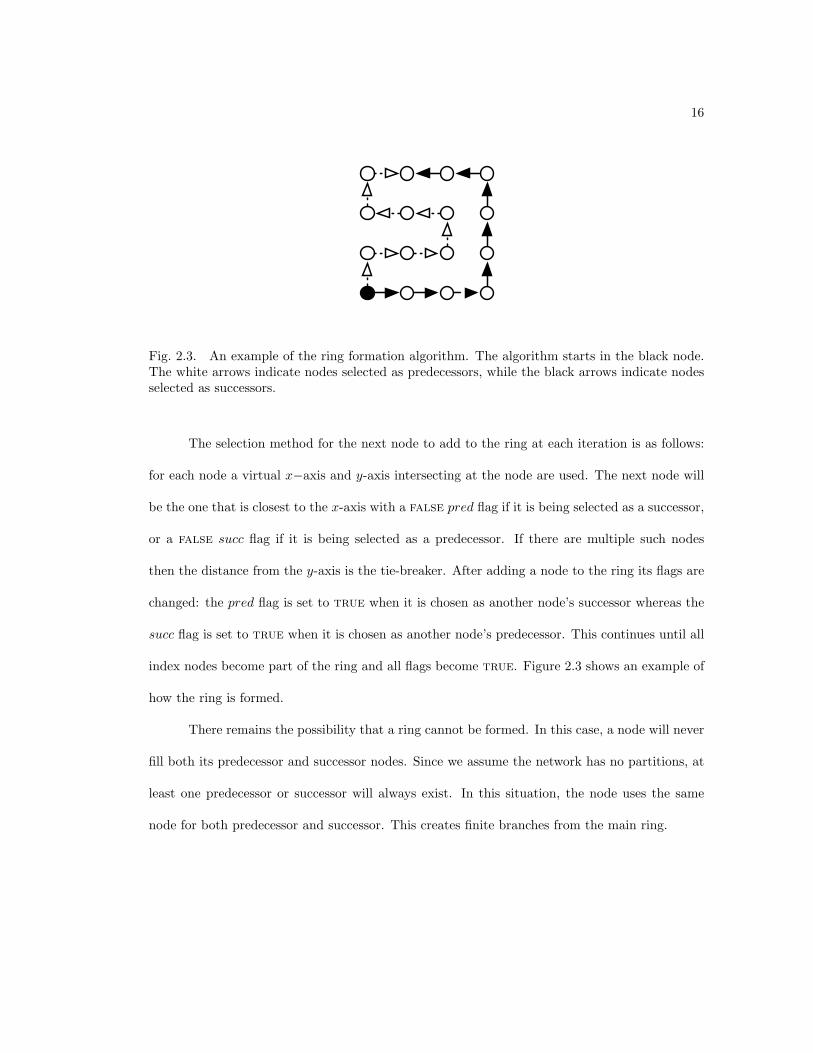
Ring formation proceeds as follows: the node that runs the ring will start by creating two

flags for each node: pred and succ. At the beginning, the flags of all nodes are set to false.

The pred flag of a node is set to true only if that node is assigned a predecessor. Similarly, the

succ flag of a node is set to true only if that node is assigned a successor. The algorithm starts

by selecting the node with the lowest ID. For that node, the two closest nodes are selected as

predecessor and successor. Flags for the three nodes are then changed accordingly. After this,

the ring starts growing from both the predecessor and successor sides in an alternating fashion,

i.e we go to the predecessor and select its predecessor and the we go to the successor and select

its successor and so on. Growing the ring from both sides ensures that the distances between

nodes is more uniform and that we do not end up with a link between two nodes that is many

hops in length.

16

Fig. 2.3. An example of the ring formation algorithm. The algorithm starts in the black node.The white arrows indicate nodes selected as predecessors, while the black arrows indicate nodesselected as successors.

The selection method for the next node to add to the ring at each iteration is as follows:

for each node a virtual x−axis and y-axis intersecting at the node are used. The next node will

be the one that is closest to the x-axis with a false pred flag if it is being selected as a successor,

or a false succ flag if it is being selected as a predecessor. If there are multiple such nodes

then the distance from the y-axis is the tie-breaker. After adding a node to the ring its flags are

changed: the pred flag is set to true when it is chosen as another node’s successor whereas the

succ flag is set to true when it is chosen as another node’s predecessor. This continues until all

index nodes become part of the ring and all flags become true. Figure 2.3 shows an example of

how the ring is formed.

There remains the possibility that a ring cannot be formed. In this case, a node will never

fill both its predecessor and successor nodes. Since we assume the network has no partitions, at

least one predecessor or successor will always exist. In this situation, the node uses the same

node for both predecessor and successor. This creates finite branches from the main ring.

17

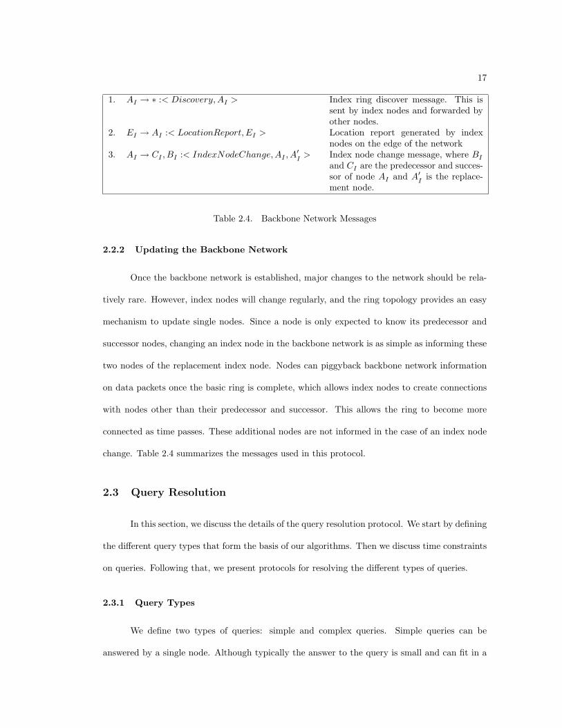
1. AI → ∗ :< Discovery, AI > Index ring discover message. This issent by index nodes and forwarded byother nodes.

2. EI → AI :< LocationReport, EI > Location report generated by indexnodes on the edge of the network

3. AI → CI , BI :< IndexNodeChange,AI , A′I

> Index node change message, where BI

and CI are the predecessor and succes-sor of node AI and A′

Iis the replace-

ment node.

Table 2.4. Backbone Network Messages

2.2.2 Updating the Backbone Network

Once the backbone network is established, major changes to the network should be rela-

tively rare. However, index nodes will change regularly, and the ring topology provides an easy

mechanism to update single nodes. Since a node is only expected to know its predecessor and

successor nodes, changing an index node in the backbone network is as simple as informing these

two nodes of the replacement index node. Nodes can piggyback backbone network information

on data packets once the basic ring is complete, which allows index nodes to create connections

with nodes other than their predecessor and successor. This allows the ring to become more

connected as time passes. These additional nodes are not informed in the case of an index node

change. Table 2.4 summarizes the messages used in this protocol.

2.3 Query Resolution

In this section, we discuss the details of the query resolution protocol. We start by defining

the different query types that form the basis of our algorithms. Then we discuss time constraints

on queries. Following that, we present protocols for resolving the different types of queries.

2.3.1 Query Types

We define two types of queries: simple and complex queries. Simple queries can be

answered by a single node. Although typically the answer to the query is small and can fit in a

18

single message, this is not always the case. For example a simple query could ask, “Where is the

item with ID #19250?” The response to this query would take only a single message, since it is

only a question of existence and location. Larger simple queries can also exist, such as, “What

are all of the items in Crate #12919?” Although this is still a simple query that can be answered

by a single node, the response is much larger than in the previous example. Note that queries

this simple can be answered by either the node that is closest to item or that node’s index node,

which can improve querying performance.

The second type of query is complex queries. In complex queries the answer must be read

and aggregated from several nodes. For example, a complex query could ask, “How many shoes

are in the warehouse?” To answer this, the query must reach all nodes with shoes or all indexing

nodes that have indexed this information. Complex queries can also combine queries, such as

finding whether an item is available, and if so, in what colors. Complex queries are much more

difficult to resolve because they require coordination and aggregation of information across the

entire warehouse. We concentrate on simple queries and leave the design and implementation of

algorithms for complex queries as future work.

2.3.2 Query Time Constraints

Every query has a time constraint, Tconstraint, within which it should be resolved. This

determines how urgent is the query. For real-time applications, Tconstraint can be set to a very

small value indicating that it requires the minimum possible delay. For low priority queries,

Tconstraint can be set to a large value indicating that it does not require any special treatment

and can be answered with a higher delay. An example of a low priority query would be nightly

inventory checks that can be batched and resolved as the robot moves around the warehouse. In

between the two extremes, time constraints can be set to any value according to the application

and its delay requirements.

19

2.3.3 Resolving Simple Queries

Query resolution for simple queries consists of three main steps: sending the query and

locating the data source, getting an initial response from the data source regarding the query

answer, deciding what the robot should do, i.e. whether it should move, and if so, to which node,

or if it should wait for the data to be sent over the network.

A query is generated by a central server and sent to the robot, R. When the robot receives

the query it sends it to the nearest index node, I. If no index node is within communication

range, the robot sends the query to the nearest node which then forwards it to an index node.

Next, the index node determines the location of the data source, D. This is done by sending

the query over the backbone network to reach all index nodes. In the ring, the query is sent in

both directions to reduce lookup time. The time it takes to locate the data source is referred to

as Tlookup. To make the lookup time faster for later queries, location information is cached as

memory is available in the index nodes. Since items can be moved, cached data has a timer after

which it must be refreshed or deleted.

Once the data source is found using the backbone, it sends a response message back to

the robot. If the queried data is small enough to fit in a single message, it is included in the

message and the query is resolved. If the data cannot fit in one message the data source still

sends a response message containing the ID, the location of the data source, and the size of the

answer, S. Along the way back to R, each node, i, in the path appends its ID and location to

the message, so the message contains a path back to the data source. Since we use geographic

based routing, this path will always be the shortest possible path in terms of physical distance.

The time it takes for the response to get back to R is Tresponse. This time includes both the

lookup time and the time needed to send the response message from D to R.

Using the information it has about the warehouse layout and the information gathered

from nodes in the path, the robot decides its next course of action. The robot has three possible

20

courses of action: it can move to the data source, request that the data source send the response

over the network to the robot’s current location, or request that the data source send the response

to an intermediary node from which the robot will pick up the data. The robot chooses its course

of action based on the query’s time constraint. The robot calculates the query resolution time,

Tquery(i), for each point i in the path between the data source and its current location. Tquery(i)

includes both the time for the data to be transferred to node i and the time it takes the robot to

physically move to node i. Obviously Tquery(i) is dominated by the robot’s moving time. Tquery(i)

must be less than the time constraint, Tconstraint. To prevent excess energy consumption, the

robot chooses the node that is the fewest hops away from the data source that the robot can

move to in time. The next section describes this process in more detail.

2.3.3.1 Determining the Query Resolution Time

To determine the query resolution time, the robot first decides from which point in the

path it is going to collect the data. First, the robot calculates the time, Ci, it would take to travel

to any node i in the path. It then calculates the time, Mi, it takes to transmit the data from

D to any node i in the path. In most cases Ci >> Mi. The robot then picks the node x which

is closest to the data source such that Tquery(i) ≤ Tconstraint. The resolution time Tquery(x)

includes the time to get the initial response from D and the larger of Cx and Tdecision + Mx.

Since the robot knows the layout of the warehouse, its current location, the location of

all nodes i on the path from the data source to the robot, and its movement speed, determining

the value of Ci for any point i is easy. To determine Mi for each node in the path, the robot

uses size of the response, S, the transfer rate of the mesh network, B, and the number of hops

between i and the data source, di and the following equation:

Mi =S

B× (di − 1) (2.1)

21

Now we consider the response time. This is equal to the time to locate the data source, Tlookup

plus the time it takes to send the response packet from D to R over dR hops:

Tresponse = Tlookup +dR

B(2.2)

Next we look at the time to send the robot’s decision back to D, which is the time it takes to

send a single packet back to D over dR hops:

Tdecision =dR

B(2.3)

Finally, the query resolution time if node x in the path is chosen is:

Tquery(x) = Tresponse + max(Tdecision + Mx, Cx) +S

B(2.4)

Recall that S is the size of the response and B is the transfer rate of the network. As mentioned

earlier, this accounts for the time to get the initial response from D, the greater of the time it

takes the robot to reach node i or the time it takes the data to reach node i, and the time needed

to get the answer (which is S packets) from i.

The robot chooses the node x that is closest to the data source such that:

Tquery(x) ≤ Tconstraint (2.5)

When x is found, the robot moves to that location and asks the data source to simultaneously

forward the data to x. If for all nodes i on the path Tquery(i) > Tconstraint, this path cannot be

used and the query cannot be resolved. This is extremely unlikely for reasonable Tconstraint, since

the robot can always choose to have the data source send the entire response over the network.

22

2.3.3.2 Protocol Outline

The following outlines the algorithm used to resolve simple queries:

1. R → I : < Query, Tconstraint > – Robot (R) sends query to nearest index node (I).

2. I : locate D – Index node locates data source (D) using backbone.

3. if S = 1 : D → s : < Answer > – if answer fits in one packet send it back to R. end.

4. else D → R : < Response, S, ID1, l1, ID2, l2, ..., IDn, ln > – D sends response messageback to R including the answer size (S), IDs and locations of intermediate nodes (1, ..., n).

5. R : selects x – R selects a node x to which the data should be forwarded according to2.3.3.1.

6. if x = R robot waits for the dataelse robot moves to x

7. if x = D data source waits for robotelse D forwards data to x

8. R → x : < Query > – Robot sends query to x

9. x → D : < Answer > – x sends answer to robot

2.3.4 Resolving Complex Queries

Although we did not fully develop algorithms for resolving complex queries, in this section

we briefly outline possible methods that can be used to resolve complex queries. As discussed

earlier, complex queries require combining data from multiple nodes in the network, which greatly

increases the complexity of the problem. It is impossible to directly apply our method for

resolving simple queries to complex queries, but we can see how it is possible to adapt our

protocol to handle data from multiple sources. For instance, suppose a query asks for the total

number of shoes in a warehouse. Assume for simplicity that all index nodes have fully indexed

the nodes for which they are responsible. Even with this simplification, this problem is incredibly

complex. The query still requires data from every single index node in the network, which could

easily number in the hundreds in a large network. The robot must choose optimal intermediary

nodes from which to pick up the data from each index node. With hundreds of index nodes and

23

thousands of possible intermediary nodes, a combinatorial explosion is inevitable, making this

problem undecidable in polynomial time.

Clearly, directly applying our simple query protocol to the complex query case is infeasible.

However, a small change to the algorithm can greatly reduce the number of possible paths the

robot could take to pick up all of the data from the warehouse. The robot can choose one or

more fusion points, where multiple nodes can send data for pickup. The number of nodes that

send data to a single fusion point is limited by the storage capacity of the fusion point, but

even multiple fusion points would vastly reduce the number of possible paths the robot can take.

Choosing a good fusion point is a difficult problem in and of itself, but it may be easier to choose

a fusion point in a connected mesh network than to choose an optimal path for a robot to travel

to hundreds of nodes.

2.4 Implementation and Simulation

Due to the lack of available active tags that matched our desired feature set, we used

Crossbow MicaZ motes to approximate active tags. They have essentially the same feature set,

with similar processing and storage limitations, so we felt that this substitution was appropriate.

The MicaZ motes run TinyOS [5], an embedded operating system designed for sensor motes.

We implemented our algorithms in TinyOS 2.0. In addition, we implemented a mobile reader

platform interfaced with a MicaZ mote. Although our implementation ran on real motes, it

was not feasible to run an actual experiment with hundreds of motes and a reader, so we used

TinyOS’s built-in simulator, TOSSIM, to simulate larger experiments with the reader and collect

results.

To test our algorithms, we simulated a small network of 150 motes in a 100 ft. × 100 ft.

warehouse and a large network of 900 motes in a 1000 ft. × 1000 ft. warehouse. We simulated

our full algorithm on each the network: each group of nodes chose an index node, indexed sample

data, and formed a backbone network. We then ran 650 queries on each network, using only

24

the mobile reader without the mesh network, our hybrid movement and transmission algorithm,

and using only the mesh network without the reader. We measured the total distance travelled

by the mobile reader, the power consumption of the network, and the success rate of queries, as

measured by the number of queries that met a randomly chosen time constraint. We also tracked

the movement of the mobile reader. Since TOSSIM does not simulate power usage, we measured

power consumption as a function of the number of transmissions a node made.

2.5 Results

It is important to keep in mind the desired benefit of using the mobile reader and mesh

network. Using only the active tag mesh network to resolve queries would reduce latency, but

this approach would also be severely limited by the battery life of the active tags. Similarly, only

using a single mobile reader that travels to each active tag to read query data would eliminate

battery life concerns, but it would also have very high latency since the reader would have to

move all the way to the tag for every query. The hybrid approach is designed to balance the

trade-off between latency and battery life.

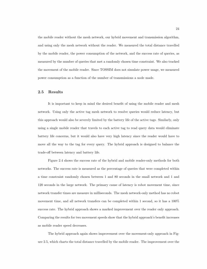
Figure 2.4 shows the success rate of the hybrid and mobile reader-only methods for both

networks. The success rate is measured as the percentage of queries that were completed within

a time constraint randomly chosen between 1 and 80 seconds in the small network and 1 and

120 seconds in the large network. The primary cause of latency is robot movement time, since

network transfer times are measure in milliseconds. The mesh network-only method has no robot

movement time, and all network transfers can be completed within 1 second, so it has a 100%

success rate. The hybrid approach shows a marked improvement over the reader only approach.

Comparing the results for two movement speeds show that the hybrid approach’s benefit increases

as mobile reader speed decreases.

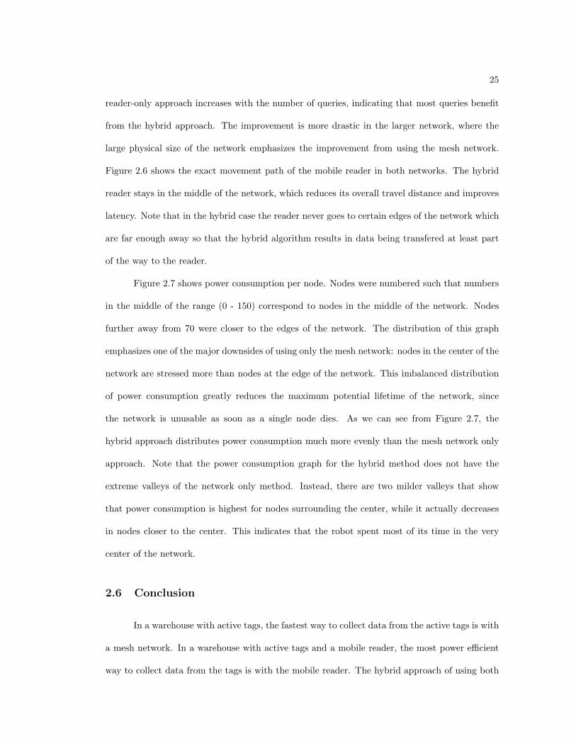
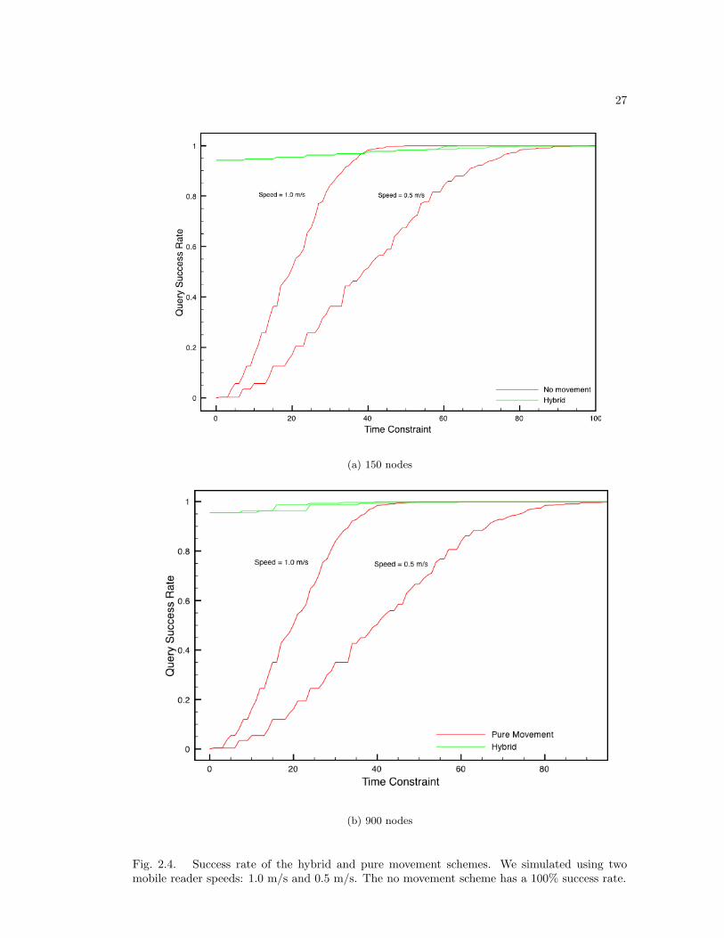
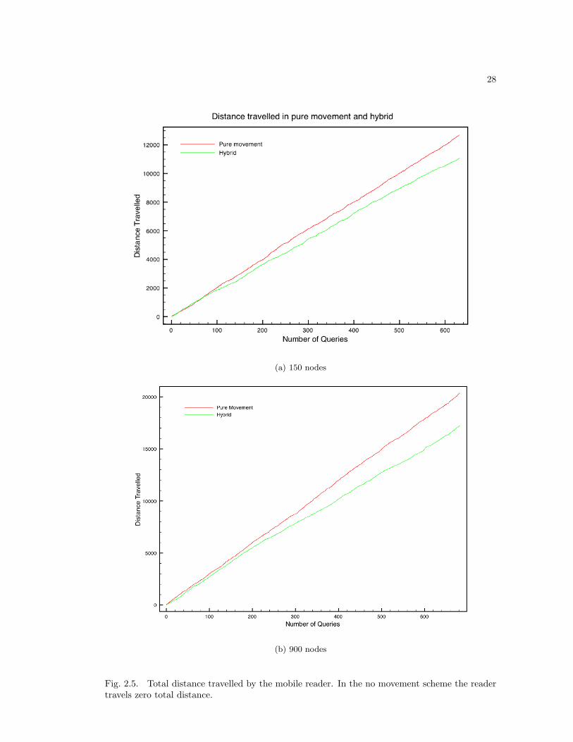
The hybrid approach again shows improvement over the movement-only approach in Fig-

ure 2.5, which charts the total distance travelled by the mobile reader. The improvement over the

25

reader-only approach increases with the number of queries, indicating that most queries benefit

from the hybrid approach. The improvement is more drastic in the larger network, where the

large physical size of the network emphasizes the improvement from using the mesh network.

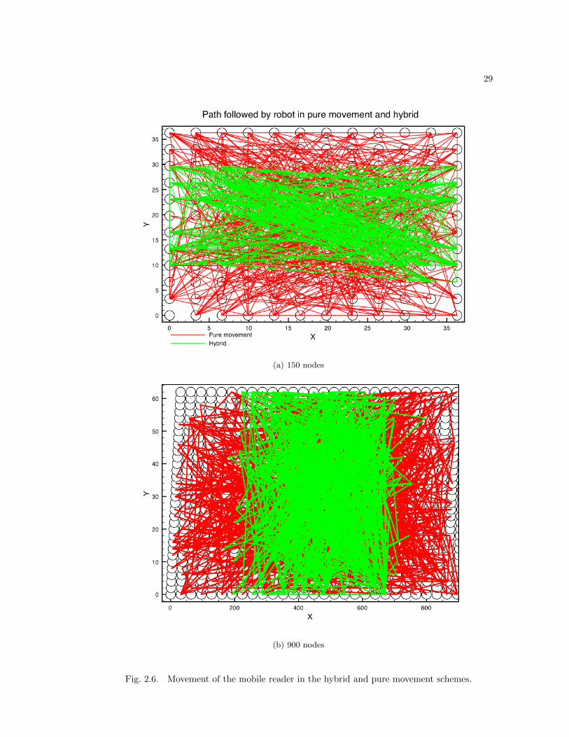
Figure 2.6 shows the exact movement path of the mobile reader in both networks. The hybrid

reader stays in the middle of the network, which reduces its overall travel distance and improves

latency. Note that in the hybrid case the reader never goes to certain edges of the network which

are far enough away so that the hybrid algorithm results in data being transfered at least part

of the way to the reader.

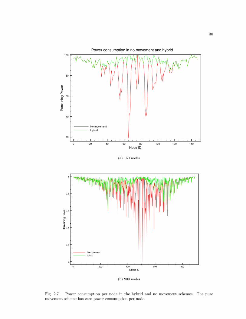
Figure 2.7 shows power consumption per node. Nodes were numbered such that numbers

in the middle of the range (0 - 150) correspond to nodes in the middle of the network. Nodes

further away from 70 were closer to the edges of the network. The distribution of this graph

emphasizes one of the major downsides of using only the mesh network: nodes in the center of the

network are stressed more than nodes at the edge of the network. This imbalanced distribution

of power consumption greatly reduces the maximum potential lifetime of the network, since

the network is unusable as soon as a single node dies. As we can see from Figure 2.7, the

hybrid approach distributes power consumption much more evenly than the mesh network only

approach. Note that the power consumption graph for the hybrid method does not have the

extreme valleys of the network only method. Instead, there are two milder valleys that show

that power consumption is highest for nodes surrounding the center, while it actually decreases

in nodes closer to the center. This indicates that the robot spent most of its time in the very

center of the network.

2.6 Conclusion

In a warehouse with active tags, the fastest way to collect data from the active tags is with

a mesh network. In a warehouse with active tags and a mobile reader, the most power efficient

way to collect data from the tags is with the mobile reader. The hybrid approach of using both

26

the mesh network and a mobile reader is neither the fastest nor the most power efficient, but it

can provide the most useful trade-off between the two.

27

(a) 150 nodes

(b) 900 nodes

Fig. 2.4. Success rate of the hybrid and pure movement schemes. We simulated using twomobile reader speeds: 1.0 m/s and 0.5 m/s. The no movement scheme has a 100% success rate.

28

(a) 150 nodes

(b) 900 nodes

Fig. 2.5. Total distance travelled by the mobile reader. In the no movement scheme the readertravels zero total distance.

29

(a) 150 nodes

(b) 900 nodes

Fig. 2.6. Movement of the mobile reader in the hybrid and pure movement schemes.

30

(a) 150 nodes

(b) 900 nodes

Fig. 2.7. Power consumption per node in the hybrid and no movement schemes. The puremovement scheme has zero power consumption per node.

31

Chapter 3

Multiple Reader Data Gathering

with Passive RFID Tags

Previously, we addressed the problem of real-time inventory tracking and querying in

an active tag network. Although we found that it was possible to successfully use active tags

networks in combination with a mobile reader to enable real-time access to inventory information,

active tags of the type required for a robust implementation are currently not in widespread use

due to prohibitive costs. We therefore turn our attention to passive RFID tags, which are cheap

and widely available, and in many cases are already used to provide some inventory tracking.

Unlike active RFID tags, passive RFID tags have no processing or networking capabilities

and can only be read by an RFID reader. Furthermore, RFID tags can only be read from within

a short range, roughly 10 feet with current technology. These limitations immediately prevent

us from adapting our work from active tags to passive tags–there is simply no way to perform

any calculations on a passive RFID tag, let alone run complex network protocols.

We can, however, adapt our mobile reader to work with passive tags instead of active

tags. A mobile reader presents a natural solution to many of the limitations of passive RFID

tags. The reader can perform any necessary computing, and the reader can move to within range

of a passive tag to read it. In essence, we can make any passive tag a part of a larger network,

with the mobile reader moving to read tags as necessary. Of course, with a mobile reader we are

limited by the speed of the reader, which can be a severe obstacle when fulfilling many queries

in large warehouses. An obvious solution to this problem is to introduce multiple mobile readers

which can communicate with each other and coordinate their movements around the warehouse

to maximize efficiency.

32

Since we are changing the architecture of our system, we must also update our assumptions.

Most importantly, in the single reader case we assume that the reader is always connected to

a base station through which it receives queries. With multiple readers, the strong assumption

that all readers are always connected to a base station is no longer necessary. It is possible to

form a multi-hop network between readers to exchange queries, thus requiring only one reader

to be connected at any time. However, since readers can move out of range of each other,

disconnections are possible between not only a reader and the query source, but also between

readers themselves. This added complexity decreases efficiency, but allows the system to be much

more flexible.

With these changes in mind, we can describe our new goal more explicitly. We consider the

problem of real-time inventory querying using passive RFID tags with multiple mobile readers

in both a fully connected network with a base station and a multi-hop, ad-hoc network. We

present algorithms for fully connected robot movement scheduling in Section 3.2, and algorithms

for multi-hop operation in Section 3.3. We simulated our algorithms and implemented them

on our existing mobile reader platform, as described in Section 3.4. Finally, we discuss our

results in Section 3.5. Before we begin our discussion of work with multiple readers, we present

a mathematical model to motivate our use of multiple readers in the next section.

3.1 Mathematical Model

To motivate our work with multiple robots, we present a rough mathematical model to

perform a cost-benefit analysis of using multiple robots versus replacing an active tag network.

We first assume an active tag network with a single mobile reader and compute its costs, which

we compare to using multiple readers with passive tags.

33

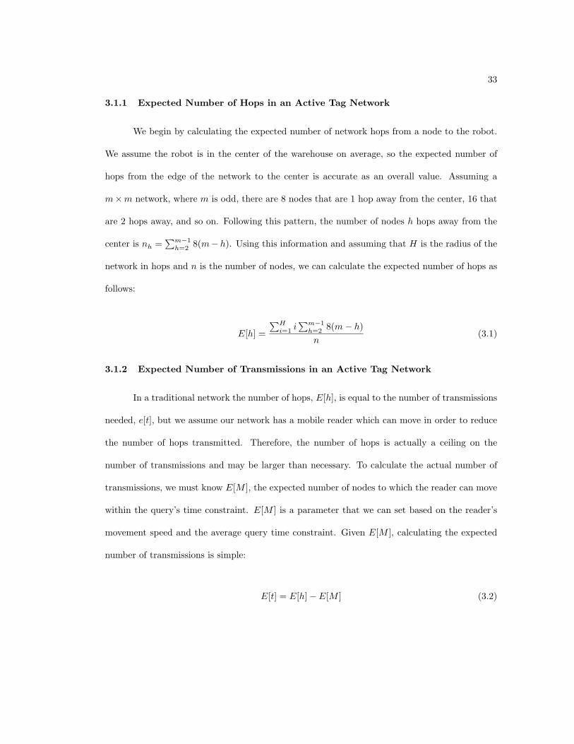
3.1.1 Expected Number of Hops in an Active Tag Network

We begin by calculating the expected number of network hops from a node to the robot.

We assume the robot is in the center of the warehouse on average, so the expected number of

hops from the edge of the network to the center is accurate as an overall value. Assuming a

m×m network, where m is odd, there are 8 nodes that are 1 hop away from the center, 16 that

are 2 hops away, and so on. Following this pattern, the number of nodes h hops away from the

center is nh =∑m−1

h=28(m− h). Using this information and assuming that H is the radius of the

network in hops and n is the number of nodes, we can calculate the expected number of hops as

follows:

E[h] =∑H

i=1i∑m−1

h=28(m− h)

n(3.1)

3.1.2 Expected Number of Transmissions in an Active Tag Network

In a traditional network the number of hops, E[h], is equal to the number of transmissions

needed, e[t], but we assume our network has a mobile reader which can move in order to reduce

the number of hops transmitted. Therefore, the number of hops is actually a ceiling on the

number of transmissions and may be larger than necessary. To calculate the actual number of

transmissions, we must know E[M ], the expected number of nodes to which the reader can move

within the query’s time constraint. E[M ] is a parameter that we can set based on the reader’s

movement speed and the average query time constraint. Given E[M ], calculating the expected

number of transmissions is simple:

E[t] = E[h]− E[M ] (3.2)

34

3.1.3 Expected Lifetime of Active Tag Network

Given the expected number of transmissions in the network, we can calculate the expected

remaining lifetime of the network based on the total energy of the network, E, the number of

queries performed, Q, and the expected number of transmissions per query, E[t].

Lifetime = E −QE[t] (3.3)

We note that when the expected remaining lifetime of the network is 0, the network has no

remaining energy. By setting Equation 3.3 to 0 and solving for Q, we can calculate the number

of queries the network can support before dying, Qf :

Qf =E

E[t](3.4)

3.1.4 Cost Analysis for Active Tag Network

Our prototype robot costs approximately $400 to build. Assuming that per-robot cost

remains the same, we can use $400 as an estimate of robot cost. Although there is not an

exact product that matches our active RFID tag currently available, other active RFID tags are

available for prices between $5 and $100. We currently use Crossbow MicaZ sensor motes as a

development testbed, which are $125 each when purchased in low quantities. Since we envision

our use of active RFID tags in high-density, high-population environments, we use $5 as our cost

estimate for active RFID tags, which is lower than the current average cost of active RFID tags.

Using our model with a E[M ] value of 30 nodes, performing 1,000,000 queries in a 10,200

node network (m = 101) requires 10,200 active tags, with a total cost of $51,000 and 1 robot

with a cost of $400. The total cost of the network is $51,400.

35

3.1.5 Cost Analysis for Passive Tag Network

Passive tags are an order of magnitude cheaper than active tags. Passive RFID tags cost

as little as $0.20 each in printable, stickered rolls of thousands. 10,200 passive RFID tags would

cost only $2,040. The number of robots required to read these tags depends largely on the

organization and distribution of the tags; a conservative estimate of 1 robot per 200 tags requires

51 robots at a total cost of $20,400. The total cost of the system is then $22,440, less than half

that of the active tag network. When labor costs for replacing active tags are considered, active

tag networks become even more expensive. With this cost analysis motivating our work, we now

consider algorithms for multiple readers.

3.2 Algorithms for Fully Connected Multiple Readers

As described earlier, the protocol has two basic steps. The first step is locating the data

source that is responsible for the desired data. The second step is collecting the data using the

mobile reader. In this section we discuss the protocol for multiple readers in a fully connected

network with a base station in full detail.

3.2.1 Locating Data Sources

Initially, we assume we know the approximate location of the data. Our motivation for

making this assumption is that warehouses are typically organized in some human-friendly fashion

in order for warehouse workers to locate items. Using this knowledge, we know roughly where

an item is and can send a mobile reader to that location to determine the precise location of the

item.

In future work we will incorporate a centralized or distributed caching scheme into our

protocol. With a cache, mobile readers can continually read tags in order to update the cache as

they move around the warehouse fulfilling queries. Furthermore, we can include other modes of

36

cache updating, such as handheld RFID readers used by warehouse workers, or readers attached

to forklifts.

3.2.2 Data Collection

After locating the tag, a robot must travel to the tag and read it to complete the query.

The robots determine which robot will retrieve the data by running our protocol. Given a

single query, choosing which robot to send is easy: we simply send the nearest robot. However,

given a distribution of queries over time, the decision of which robot to send becomes more

difficult. For instance, consider a highly skewed distribution with hotspots that are clustered

physically, temporally, or both. Hotspots can occur if a particular item or class of items is on

sale, which increases customer interest, and accordingly the number of queries for those items.

In a distribution with hotspots, it may be optimal to keep a robot in the hotspot that will not

respond to queries outside the hotspot. The difficulty here lies in determining when a hotspot

is occurring. Since we have no knowledge of future queries, we must rely on heuristics based on

past queries. We introduce two concepts, areas of responsibility and rest points, to heuristically

determine when a hotspot is occurring.

3.2.2.1 Areas of Responsibility

When queries are uniformly distributed, any particular reader will respond to queries from

a large area. A simple example is four readers in a square warehouse. Each reader should be

responsible for an area roughly equivalent to a quadrant. However, when a hotspot occurs, we

can reasonably expect that the hotspot will be smaller than a quadrant. The exact size of a

hotspot depends on a number of other factors, such as warehouse organization, type of hotspot,

and duration of the hotspot; since by definition a hotspot is a clustering of queries, we can assume

that the hotspot will be fairly small. The concept of areas of responsibilities attempts to measure

37

the average area a reader stays within. If this area is small enough, we can assume a reader is in

a hotspot, and act accordingly.

A reader’s area of responsibility is the range within which the reader will respond to

queries. An area of responsibility is described as a circle of radius ARr, centered upon either the

reader itself, r, or the reader’s rest point, RPr (described below). Since areas of responsibilities

are circles, they will not provide full coverage in a rectangular warehouse, and there will be

overlap between the areas of responsibilities of different readers. In these cases, we revert back

to the simple method of sending the closest robot.

The value of ARtr, the area of responsibility radius at time t, is determined by the weighted

moving average of the distance reader r travels, dr:

ARtr

= α(dr) + (1− α)ARt−1r

Where ARt−1r

is the previous value of ARr, dr is the distance the reader travelled to read the

last tag it was chosen to read, and α is a parameter. Experimentally, we have found that a value

of α = 0.1 works well.

3.2.2.2 Rest Points

Once a reader’s area of responsibility is determined, the question of where to center the

area of responsibility arises. The area of responsibility can be centered on some fixed point,

such as the reader’s starting location, or it can be centered on the robot itself. If the area of

responsibility is centered on a fixed point, while it may accurately reflect the size of a hotspot, it

in no way reflects the location of the hotspot. Meanwhile, if the area of responsibility is centered

on the reader itself, it may move too quickly and erratically to reflect the true location of the

hotspot. A compromise between the two, a moving average of the reader’s location, is needed.

38

We determine a reader’s rest point, RPr, using the reader’s average location over a number

of queries, rp recalculate, with maximal outliers removed. We remove outliers to eliminate the

effect of single queries that lie far away from a robot’s normal roaming area. rp recalculate is a

parameter; experiments have shown 15 to be an appropriate value.

It should be noted that a reader does not return to its rest point after each query. Rather,

the rest point is the point on which the reader’s area of responsibility is centered. As described

in the next section, in our standard protocol the reader can move out of its area of responsibility

if necessary to fulfill a query, but will always return to the area of responsibility after fulfilling

the query. Further note that in some of the protocol variations described in Section 3.2.4, the

area of responsibility is centered on the reader itself; in these cases the reader can never leave its

area of responsibility and the rest point is meaningless.

3.2.3 Fully Connected Protocol

We now describe in detail the protocol that the mobile readers follow.

1. A query is sent to all of the robots via a base station from a centralized server.

2. Since we assume the location of all queries is known, we immediately proceed to choosing

a robot to retrieve the data. There are three cases:

• The query is in one and only one robot’s area of responsibility. This robot is chosen

to retrieve the data.

• The query is in no robots’ area of responsibility. The nearest robot is chosen to retrieve

the data.

• The query is in more than one robot’s area of responsibility. Of the robots in whose

areas of responsibilities the query is located, the closest one is chosen to retrieve the

data.

39

3. Once the chosen robot arrives at the data location, it reads the RFID tag and sends the

information back to the server via the base station. At this point it also updates its area of

responsibility using the equation above, and updates its rest point if rp recalculate queries

have passed since it last changed its rest point.

4. If the robot has moved outside its area of responsibility, it now moves back to the closest

point within the area of responsibility.

3.2.4 Fully Connected Protocol Variations

In addition to the original protocol above, we developed a number of variants on the

protocol for comparison purposes.

Simple In this variation, we ignore both areas of responsibilities and rest points and simply

choose the closest robot. Robots rest wherever their last query put them.

AR + RP This is the protocol described in 3.2.3

AR Only In this variation, we only adjust and follow the area of responsibility, which is always

centered on the robot. There are no rest points. Since the area of responsibility is centered

on the robot itself, it can never leave its area of responsibility.

Flexible Grid This is similar to the AR Only protocol, but the areas of responsibilities are

fixed on each robot’s starting location. Like the AR Only protocol, there are no rest

points. Unlike the AR Only protocol, robots can leave their areas of responsibility, and

must return to them if they do.

RP Only In this variation, we only adjust rest points. The area of responsibility is of fixed size

and centered on the rest point.

Return to Center In this variation, the robot always returns to its origin location after re-

sponding to a query. Areas of responsibilities and rest points are ignored.

40

3.3 Algorithms for Multi-hop Connected Multiple Readers

Although it is easy to simulate a warehouse where mobile readers are always connected

with a central server and have perfect information about the network, that will not always be

the case in an actual deployment. Real-time inventory systems are often designed with military

use in mind, since the constraints of a battlefield often requires that warehouses be quickly

constructed with little time to deploy proper infrastructure. In this case, it is easy to imagine a

battlefield storage area that contains thousands of RFID-tagged items but no wireless networking

infrastructure. If there are no wireless base stations, the mobile readers must rely on a multi-hop

mesh network in order to communicate.

Queries must still originate from outside the mobile readers, for example, from a wireless-

equipped laptop connected to the mesh network at the edge of the warehouse. Furthermore,

queries can no longer be sent to all readers—they can only be sent to whatever readers are in

range of the query source. Therefore, queries must either be saved by the readers that are in

range and transmitted to the other readers at a later time, or the querying algorithms must be

run on an incomplete set of readers.

With these changes to the underlying network, in multi-hop operation we can no longer

assume readers have perfect information about the network. Indeed, because of disconnections

readers often have very poor information about the network. It is only safe to assume that a

reader will know the location of itself and nodes it is connected to via the mesh network, which

makes it inefficient to use our mobile reader algorithms without modification, since they assume

all the readers know the locations of all of the other readers. Furthermore, since queries now

originate from specific locations, and not from a central server to which all readers have access,

once a query has been fulfilled, the reader must transmit the result back to the query source.

We made a number of additions to our assumptions and algorithms in order to accommo-

date the differences between multi-hop and centralized operation. In our simulation, queries now

41

originate from locations on the edge of the warehouse. The locations are uniformly distributed

across all four sides of the warehouse and the location from which a query originates is chosen

at random. Additionally, query responses must be transferred back to the originating location

before a query is considered complete. While it may be possible that a query source is in range

of no readers, we assume that queries can only originate from query sources that are in range of

readers. To simulate multi-hop operation, we must be able to determine if readers are in wireless

communication range of each other and query sources. We use a wireless range parameter, set

to 300 feet to reflect current wireless technology, to simulate wireless disconnections.

Since queries originate from a specific location and the querying algorithms only run on

the readers that receive the query, it is often the case that the reader responding to a query is not

the optimal reader. In order to counter this inefficiency, as a reader moves to a query location,

it periodically searches for other readers. If it locates another reader that is closer to the query

location than it is, it transfers the query to that reader via the mesh network. This cascading

effect greatly reduces the distance readers must travel to fulfill queries. This effect combined with

limited wireless range increases the usefulness of locality and increases the performance of the

flexible grid and rest point algorithms relative to the naive and areas of responsibility algorithms.

Figure 3.1 illustrates this cascade effect.

In order to transmit queries responses back to their corresponding query sources, we

introduce a query return stage to all algorithms. Upon reading an RFID tag and obtaining a

query result, readers return to the query source location while continuously searching for other

readers that are closer to the query source, as they do when moving to read queries. The cascading

effect once again reduces moving distance. Once a reader is within wireless range of the query

source, it can transmit the query result back to the source and the query is considered answered.

In the next section we present updated protocols that reflect these changes.

42

3.3.1 Multi-hop Protocol

The base multi-hop protocol is described in detail below.

1. A query is broadcast from a query origin point such as a laptop on the edge of the network.

All robots in range of the broadcast will react to the query. We assume at least one robot

is in range of the broadcast.

2. If a robot in broadcast range of the query origin point is connected to any other robots, it

forwards the query information to those robots.

3. As with the fully connected protocol, we assume the location of the query is known. We

proceed to choosing which robot will respond to the query. The basic protocol for choosing

which robot will respond to the query is the same as in the fully connected case. However,

since the robots are not fully connected, only robots that received the query take part in

the protocol. As before, there are three cases:

• The query is in one and only one robot’s area of responsibility. This robot is chosen

to retrieve the data.

• The query is in no robots’ area of responsibility. The nearest robot is chosen to retrieve

the data.

• The query is in more than one robot’s area of responsibility. Of the robots in whose

areas of responsibilities the query is located, the closest one is chosen to retrieve the

data.

4. Once a robot is chosen to respond to the query, it begins to move to the data location.

While it is moving, it periodically pings for other robots in its wireless range. If a robot that

is closer to the data location than the current chosen robot responds, the current chosen

robot forwards the query information to that robot and returns to its area of responsibility.

The new robot repeats this process until a robot reaches the data location.

43

5. Once the chosen robot arrives at the data location, it reads the RFID tag. The robot must

now transfer the response to the query origin point. If the query origin point is within

broadcast range, the robot simply sends the response over the network. If the query origin

point is not within broadcast range, the robot begins to move back to the query origin

point.

6. As the robot is moving back to the query origin point, it periodically pings for other robots

in its wireless range. If a robot that is closer to the query origin point than the current

robot responds, the current robot forwards the query response to that robot and returns to

its area of responsibility. The new robot repeats this process until a robot is within range

of the query origin point.

7. Once a robot is within wireless range of the query origin point, it transmits the query

response to the query origin point, completing the query.

8. Every time a robot forwards query data, it updates its area of responsibility using the

equation above, and updates its rest point if rp recalculate queries have passed since it

last changed its rest point.

3.3.2 Multi-hop Protocol Variations

The protocol variations we developed for the fully connected case also apply to the multi-

hop case. The variant protocols are the same as in the fully connected case, but with the addition

of query and response forwarding between robots.

3.4 Implementation and Simulation

To test our algorithms, we both implemented and simulated them. We simulated and

tuned our algorithms using a custom Python simulation that modeled thousands of passive tags

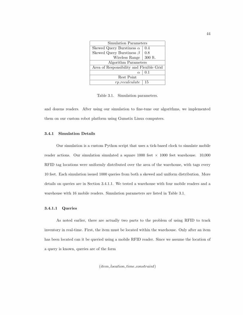
44

Simulation ParametersSkewed Query Burstiness α 0.4Skewed Query Burstiness β 0.8

Wireless Range 300 ft.Algorithm Parameters

Area of Responsibility and Flexible Gridα 0.1

Rest Pointrp recalculate 15

Table 3.1. Simulation parameters.

and dozens readers. After using our simulation to fine-tune our algorithms, we implemented

them on our custom robot platform using Gumstix Linux computers.

3.4.1 Simulation Details

Our simulation is a custom Python script that uses a tick-based clock to simulate mobile

reader actions. Our simulation simulated a square 1000 feet × 1000 feet warehouse. 10,000

RFID tag locations were uniformly distributed over the area of the warehouse, with tags every

10 feet. Each simulation issued 1000 queries from both a skewed and uniform distribution. More

details on queries are in Section 3.4.1.1. We tested a warehouse with four mobile readers and a

warehouse with 16 mobile readers. Simulation parameters are listed in Table 3.1.

3.4.1.1 Queries

As noted earlier, there are actually two parts to the problem of using RFID to track

inventory in real-time. First, the item must be located within the warehouse. Only after an item

has been located can it be queried using a mobile RFID reader. Since we assume the location of

a query is known, queries are of the form

(item, location, time constraint)

45

Where item is the item we are searching for, location is the item’s location, and time constraint

is an optional time constraint on the query.

Although our system and algorithms can be used to answer individual queries, it is more

interesting to look at an overall distribution of queries over time. There are two basic distributions

of queries over a warehouse: uniform and skewed. A uniform distribution is simple: queries are

uniformly distributed over the entire warehouse area. This could occur in a warehouse where

items are very well distributed and no particular item is more or less popular than average.

In a real warehouse, however, it is likely that some items will be more popular than others

and will therefore be queried more often. For instance, if a store is having a sale on a particular

brand of shoes, the area where those shoes are located will be more heavily loaded with queries.

In this case, we say the queries have a skewed distribution, and that a hotspot has developed in

shoe department.

When queries are uniformly distributed, all readers will respond to queries from a large

area. A simple example is four readers in a square warehouse. Each reader should be responsible

for an area roughly equivalent to a quadrant. However, a hotspot must be a concentration of many

queries in a short of amount of time in a smaller than average area in order to be distinguished

from uniformly distributed queries.

The exact shape and size of a hotspot depends on a number of outside factors, such as

warehouse organization, cause of the hotspot, and duration of the hotspot, but since a hotspot

is defined as a noticeable clustering of queries, we can assume that the hotspot will be distin-

guishably small. In many ways a skewed distribution is more interesting to study than a uniform

distribution: identifying when a skew or hotspot occurs is important and non-trivial, and opti-

mal robot movement can be greatly affected by a skew. With this in mind, our algorithms are

designed to accommodate both skewed and uniform queries.

We used two algorithms to shape the skewed query distribution: a burstiness algorithm

and the Zipf distribution [6]. We used the burstiness algorithm to determine when to begin

46

a burst of queries in the hotspot. Within the hotspot, queries were distributed using the Zipf

distribution.

The burstiness algorithm is:

• If not in burst, enter a burst with probability α, remain not in a burst with probability

1− α

• If in a burst, remain in the burst with probability β, leave the burst with probability 1− β

α and β are parameters, our simulations were run using α = 0.4 and β = 0.8.

The Zipf distribution is a commonly used distribution that models elements discretely

distributed with a power law. The exact formula is:

f(k, θ,N) =1/kθ∑N

n=11/nθ

Where N is the total number of elements, k is the rank of the given element, and θ is a parameter

that characterizes the distribution. We used θ = 40 to indicate a highly skewed distribution.

3.5 Results

In this section we present simulation results for both fully connected and multi-hop algo-

rithms.

3.5.1 Fully Connected Results

Our results for four readers are shown in Figure 3.2 and results for 16 readers are in

Figure 3.3. In the skewed and uniform case we find that the naive algorithm gives the best

performance. To understand why, it is important to understand how each algorithm operates.

The naive algorithm is actually very efficient: it sends the closest reader to respond to each

query, and the readers make no extraneous movements after responding to queries. Areas of

47

responsibility, flexible grid, and rest points all require non-optimal reader choices and extraneous

movements. Our design intention for those algorithms was to to preserve reader locality around

a hotspot. Each algorithm was designed to keep one reader in a hotspot and force other readers

to answer that reader’s queries so it would not have to leave the hotspot.

Unfortunately, the loss of efficiency from forcing non-optimal reader choices and super-

fluous movement was greater than any gain in efficiency from keeping a reader in a hotspot.

Figures 3.4 and 3.5 show that the total distance traveled by each reader for the area of respon-

sibility, flexible grid, and rest point algorithms is uniformly higher than the distance traveled

for the naive algorithm. Moreover, there is a direct relationship between an increase in distance

traveled and an increase in average time per query.

Increasing the number of readers decreased overall time per query, but did not cause drastic

changes in the relative performance of the algorithms. The performance differences between the

algorithms, which was generally under 10% in the four reader case shrinks even more in the 16

reader case. It is important to note that although our algorithms performed worse than the

naive algorithm in the centralized case, the performance delta is very small. Furthermore, the

increased locality of our algorithms becomes important in multi-hop operation.

3.5.2 Multi-hop Results

Multi-hop results are shown in Figure 3.6. Although in the fully connected, centralized

mode of operation no algorithm performed markedly better than the others, in the multi-hop

case the flexible grid algorithm is clearly the best performer.

Figures 3.7 and 3.8 show the distance travelled by the readers in each algorithm. Figure 3.7

shows the total distance travelled by all readers over the entire run of the simulation. Again, the

flexible grid algorithm clearly outperforms the others. Figure 3.8 shows the secondary distance

all readers travelled over the simulation. The secondary distance measures distance travelled by

a reader after receiving a forwarded query from another reader.

48

3.6 Analysis

In the multiple reader system, we found dramatic performance differences between our

reader scheduling algorithms in the multi-hop case. In this section we formalize the differences

between algorithms in the multi-hop case in order to provide a clearer understanding of the

benefits of our algorithms and the differences between them.

3.6.1 Secondary Distance

We introduced secondary distance in Section 3.5.2, where we used it as one performance

measure of our algorithms. Here we formalize our argument for using secondary distance as a

performance measure and analyze its effects on overall performance.

As defined earlier, secondary distance is any distance a robot moves when it is not the

original recipient of a query. Consider the simple example in Figure 3.9 with three readers: A,

B, and C. Robot A receives a query from an external source, then forwards it to robot B, which

then forwards it to robot C, which reads the tag. The distances robots B and C moved are both

secondary distances. Similarly, when returning a query to the query origin, any distance moved

by robots that were forwarded the query response is a secondary distance.

To begin our analysis, we first define d1, the primary distance. In the single-hop case,

this is simply the distance from the closest reader to the RFID tag. In the multi-hop case, this

is the distance from the first robot that received the query to the RFID tag. If that robot does

not encounter any robots that are closer to the tag, then the primary distance is also the total

distance travelled to read the tag. If the robot does forward the query, we define the distance the

first robot travelled before forwarding the query as d′1, and the remaining distance to the tag as

d⊥1

= d1 − d′1. For simplicity, we discuss only the distance travelled from the query origin to the

tag, and not the distance travelled from the tag back to the query origin. A symmetric analysis

can be carried out for the return case.

49

Next, we define ds, the secondary distance. ds is the sum of any distance travelled by

robots that are not the original receivers of a query. The distance travelled by the second robot

is d2, by the third d3, and so on, with the last robot’s distance defined as dn. Then we have the

following definition of ds:

ds =n∑

i=2

di

With ds defined, we can determine the distance saved by forwarding a query, df :

df = d⊥1− ds

d⊥1

should always be less than ds, since queries are only forwarded if the second robot is closer

to the tag.

Finally, we define the total distance travelled for a query, dt:

dt = d′1

+ ds

3.6.2 Results Analysis

In the previous section we defined the secondary distance, ds. Now we examine the results

to determine how much influence secondary distance has on overall performance. We compare

the results of the naive algorithm, which performed best in the single-hop case with those of the

flexible grid algorithm, which performed best in the multi-hop case.

Table 3.2 shows aggregate values of dt, ds, and df for the naive and flexible grid algorithms,

as well as the percentage of total movement that was due to secondary movement and the total

number of handoffs from one robot to another. These results show that secondary movement

was the primary contributor to total distance travelled in both algorithms, but significantly more

so in the naive case than in the flexible grid case. While secondary movement contributed 85%

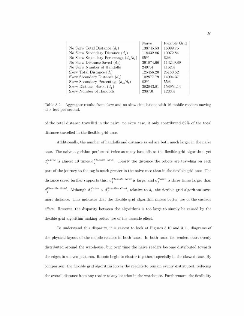
50

Naive Flexible GridNo Skew Total Distance (dt) 138745.53 16099.75No Skew Secondary Distance (ds) 118432.86 10072.84No Skew Secondary Percentage (ds/dt) 85% 62%No Skew Distance Saved (df ) 391874.66 113249.89No Skew Number of Handoffs 2497.4 1162.4Skew Total Distance (dt) 125456.20 25153.52Skew Secondary Distance (ds) 102877.79 14004.37Skew Secondary Percentage (ds/dt) 82% 55%Skew Distance Saved (df ) 382843.81 158954.14Skew Number of Handoffs 2387.0 1233.4

Table 3.2. Aggregate results from skew and no skew simulations with 16 mobile readers movingat 3 feet per second.

of the total distance travelled in the naive, no skew case, it only contributed 62% of the total

distance travelled in the flexible grid case.

Additionally, the number of handoffs and distance saved are both much larger in the naive

case. The naive algorithm performed twice as many handoffs as the flexible grid algorithm, yet

dNaives

is almost 10 times dFlexible Grids

. Clearly the distance the robots are traveling on each

part of the journey to the tag is much greater in the naive case than in the flexible grid case. The

distance saved further supports this: dFlexible Gridf

is large, and dNaivef

is three times larger than

dFlexible Gridf

. Although dNaivef

> dFlexible Gridf

, relative to dt, the flexible grid algorithm saves

more distance. This indicates that the flexible grid algorithm makes better use of the cascade

effect. However, the disparity between the algorithms is too large to simply be caused by the

flexible grid algorithm making better use of the cascade effect.

To understand this disparity, it is easiest to look at Figures 3.10 and 3.11, diagrams of

the physical layout of the mobile readers in both cases. In both cases the readers start evenly

distributed around the warehouse, but over time the naive readers become distributed towards

the edges in uneven patterns. Robots begin to cluster together, especially in the skewed case. By

comparison, the flexible grid algorithm forces the readers to remain evenly distributed, reducing

the overall distance from any reader to any location in the warehouse. Furthermore, the flexibility

51

of the flexible grid algorithm allows readers to settle in positions where they provide the maximal

benefit in terms of handoffs. Readers in the center of the warehouse position themselves such

that readers from either edge quickly hand off queries to readers in the center. While this may

occur in the naive algorithm, the lack of structure in the algorithm seems to prevent readers from

finding such positions.

Although we only compared the flexible grid and naive algorithms, our results show that

the AR only, RP only, AR + RP, and RTC algorithms performed similarly to the naive algorithm.

An interesting artifact of the analysis of the flexible grid algorithm is that the steady state

in which the readers settle near the end of the simulation has readers in the center forwarding

queries while moving very little. This indicates that a system using both fixed and mobile readers

may perform well.

3.7 Conclusion

Our results have shown that in the fully connected case, the naive algorithm performs

the best, although the remaining algorithms performed very closely to the naive algorithm, with

only a 5% performance difference between most algorithms. In the multi-hop case, the flexible

grid algorithm is the clear winner, with the readers moving up to 80% less distance than the

naive algorithm. This is a vast improvement, and makes the flexible grid algorithm the overall

best-performing algorithm. Although the naive algorithm is superior in the fully connected case,

if there is any chance that a base station will not be available, the flexible grid algorithm is the

best choice.

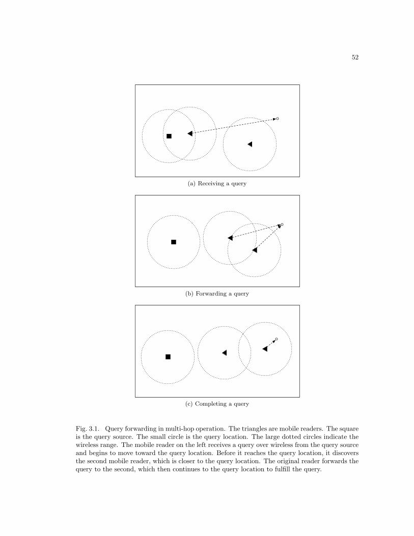
52

(a) Receiving a query

(b) Forwarding a query

(c) Completing a query

Fig. 3.1. Query forwarding in multi-hop operation. The triangles are mobile readers. The squareis the query source. The small circle is the query location. The large dotted circles indicate thewireless range. The mobile reader on the left receives a query over wireless from the query sourceand begins to move toward the query location. Before it reaches the query location, it discoversthe second mobile reader, which is closer to the query location. The original reader forwards thequery to the second, which then continues to the query location to fulfill the query.

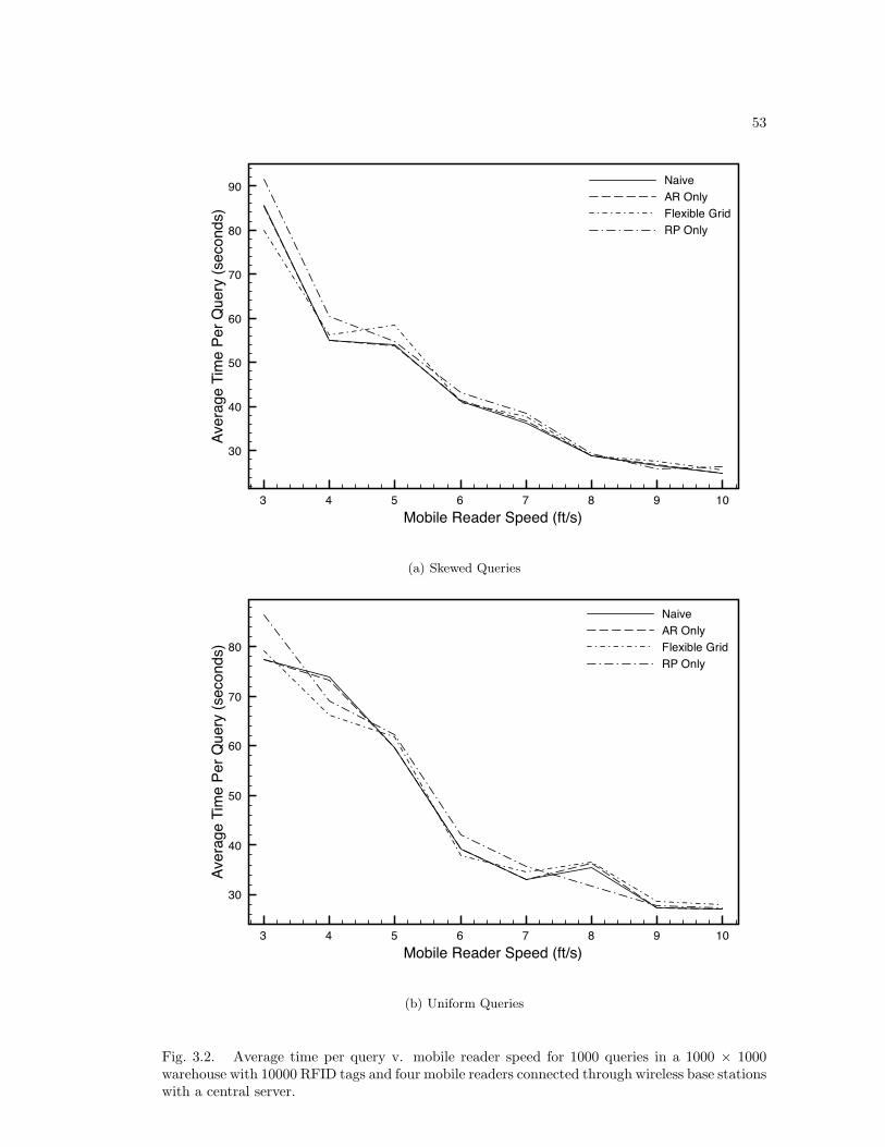
53

3 4 5 6 7 8 9 10Mobile Reader Speed (ft/s)

30

40

50

60

70

80

90

Aver

age

Tim

e Pe

r Que

ry (s

econ

ds)

NaiveAR OnlyFlexible GridRP Only

(a) Skewed Queries

3 4 5 6 7 8 9 10Mobile Reader Speed (ft/s)

30

40

50

60

70

80

Aver

age

Tim

e Pe

r Que

ry (s

econ

ds)

NaiveAR OnlyFlexible GridRP Only

(b) Uniform Queries

Fig. 3.2. Average time per query v. mobile reader speed for 1000 queries in a 1000 × 1000warehouse with 10000 RFID tags and four mobile readers connected through wireless base stationswith a central server.

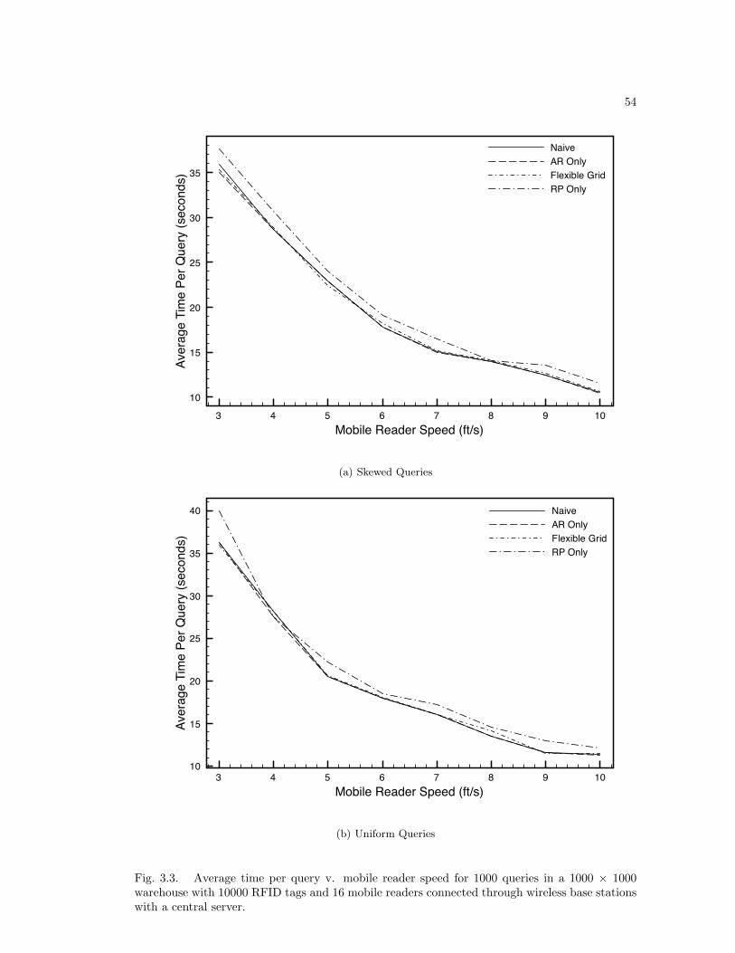
54

3 4 5 6 7 8 9 10Mobile Reader Speed (ft/s)

10

15

20

25

30

35Av

erag

e Ti

me

Per Q

uery

(sec

onds

)

NaiveAR OnlyFlexible GridRP Only

(a) Skewed Queries

3 4 5 6 7 8 9 10Mobile Reader Speed (ft/s)

10

15

20

25

30

35

40

Aver

age

Tim

e Pe

r Que

ry (s

econ

ds)

NaiveAR OnlyFlexible GridRP Only

(b) Uniform Queries

Fig. 3.3. Average time per query v. mobile reader speed for 1000 queries in a 1000 × 1000warehouse with 10000 RFID tags and 16 mobile readers connected through wireless base stationswith a central server.

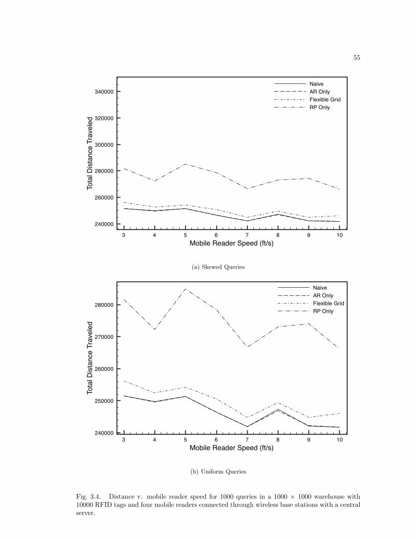
55

3 4 5 6 7 8 9 10Mobile Reader Speed (ft/s)

240000

260000

280000

300000

320000

340000To

tal D

istan

ce T

rave

led

NaiveAR OnlyFlexible GridRP Only

(a) Skewed Queries

3 4 5 6 7 8 9 10Mobile Reader Speed (ft/s)

240000

250000

260000

270000

280000

Tota

l Dist

ance

Tra

vele

d

NaiveAR OnlyFlexible GridRP Only

(b) Uniform Queries

Fig. 3.4. Distance v. mobile reader speed for 1000 queries in a 1000 × 1000 warehouse with10000 RFID tags and four mobile readers connected through wireless base stations with a centralserver.

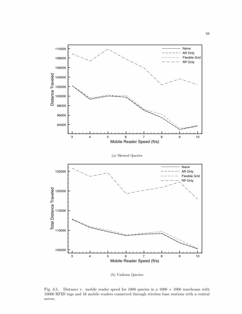
56

3 4 5 6 7 8 9 10Mobile Reader Speed (ft/s)

94000

96000

98000

100000

102000

104000

106000

108000

110000Di

stan

ce T

rave

led

NaiveAR OnlyFlexible GridRP Only

(a) Skewed Queries

3 4 5 6 7 8 9 10Mobile Reader Speed (ft/s)

105000

110000

115000

120000

125000

Tota

l Dist

ance

Tra

vele

d

NaiveAR OnlyFlexible GridRP Only

(b) Uniform Queries

Fig. 3.5. Distance v. mobile reader speed for 1000 queries in a 1000 × 1000 warehouse with10000 RFID tags and 16 mobile readers connected through wireless base stations with a centralserver.

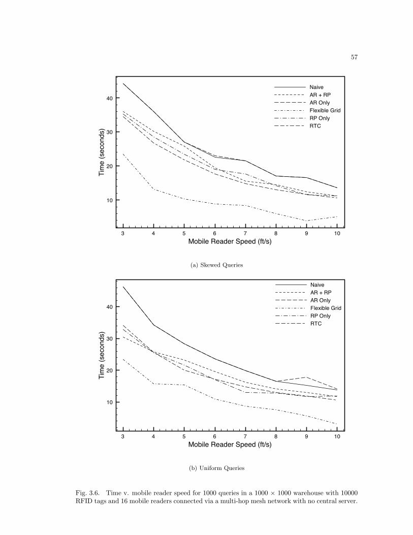
57

3 4 5 6 7 8 9 10Mobile Reader Speed (ft/s)

10

20

30

40Ti

me

(sec

onds

)

NaiveAR + RPAR OnlyFlexible GridRP OnlyRTC

(a) Skewed Queries

3 4 5 6 7 8 9 10Mobile Reader Speed (ft/s)

10

20

30

40

Tim

e (s

econ

ds)

NaiveAR + RPAR OnlyFlexible GridRP OnlyRTC

(b) Uniform Queries

Fig. 3.6. Time v. mobile reader speed for 1000 queries in a 1000 × 1000 warehouse with 10000RFID tags and 16 mobile readers connected via a multi-hop mesh network with no central server.

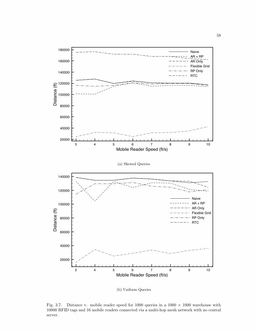
58

3 4 5 6 7 8 9 10Mobile Reader Speed (ft/s)

20000

40000

60000

80000

100000

120000

140000

160000

180000Di

stan

ce (f

t)NaiveAR + RPAR OnlyFlexible GridRP OnlyRTC

(a) Skewed Queries

3 4 5 6 7 8 9 10Mobile Reader Speed (ft/s)

20000

40000

60000

80000

100000

120000

140000

Dist

ance

(ft)

NaiveAR + RPAR OnlyFlexible GridRP OnlyRTC

(b) Uniform Queries

Fig. 3.7. Distance v. mobile reader speed for 1000 queries in a 1000 × 1000 warehouse with10000 RFID tags and 16 mobile readers connected via a multi-hop mesh network with no centralserver.

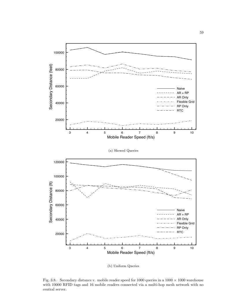
59

3 4 5 6 7 8 9 10Mobile Reader Speed (ft/s)

20000

40000

60000

80000

100000Se

cond

ary

Dist

ance

(fee

t)

NaiveAR + RPAR OnlyFlexible GridRP OnlyRTC

(a) Skewed Queries

3 4 5 6 7 8 9 10Mobile Reader Speed (ft/s)

20000

40000

60000

80000

100000

120000

Seco

ndar

y Di

stan

ce (f

t)

NaiveAR + RPAR OnlyFlexible GridRP OnlyRTC

(b) Uniform Queries

Fig. 3.8. Secondary distance v. mobile reader speed for 1000 queries in a 1000 × 1000 warehousewith 10000 RFID tags and 16 mobile readers connected via a multi-hop mesh network with nocentral server.

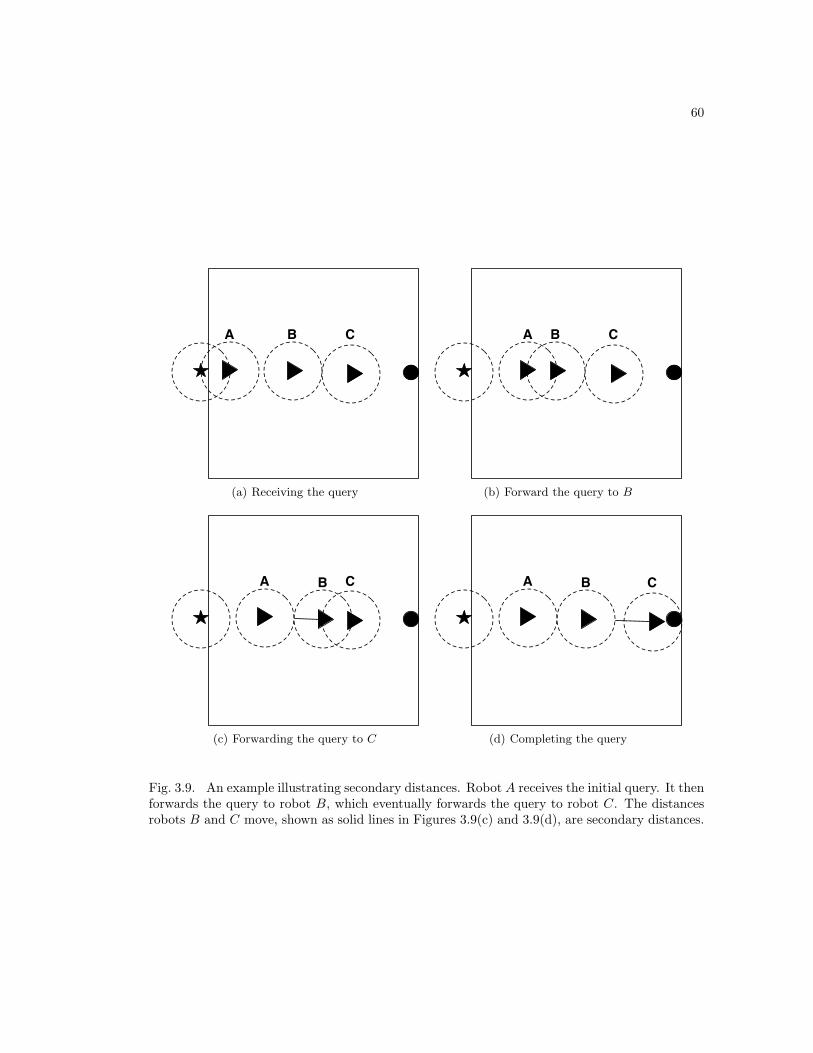
60

A

A B C

(a) Receiving the query

A

A B C

(b) Forward the query to B

A

A B C

(c) Forwarding the query to C

A

A B C

(d) Completing the query

Fig. 3.9. An example illustrating secondary distances. Robot A receives the initial query. It thenforwards the query to robot B, which eventually forwards the query to robot C. The distancesrobots B and C move, shown as solid lines in Figures 3.9(c) and 3.9(d), are secondary distances.

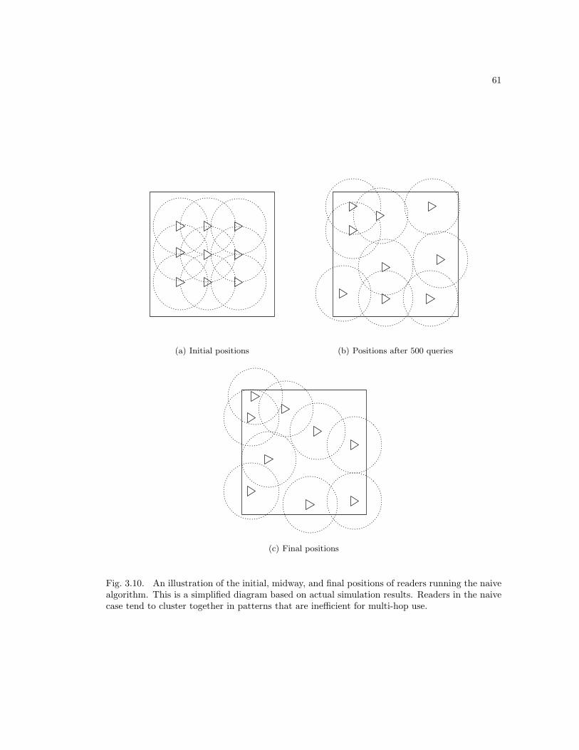
61

(a) Initial positions (b) Positions after 500 queries

(c) Final positions

Fig. 3.10. An illustration of the initial, midway, and final positions of readers running the naivealgorithm. This is a simplified diagram based on actual simulation results. Readers in the naivecase tend to cluster together in patterns that are inefficient for multi-hop use.

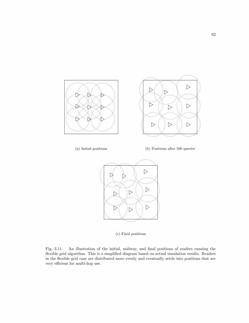
62

(a) Initial positions (b) Positions after 500 queries

(c) Final positions

Fig. 3.11. An illustration of the initial, midway, and final positions of readers running theflexible grid algorithm. This is a simplified diagram based on actual simulation results. Readersin the flexible grid case are distributed more evenly and eventually settle into positions that arevery efficient for multi-hop use.

63

Chapter 4

Conclusion

RFID has seen widespread acceptance as a means of tracking inventory in warehouses, but

technological limitations have prevented its use in real-time inventory tracking. We presented two

methods of adopting both newer active RFID technology and existing passive RFID technology

to real-time inventory systems. Key to both of these solutions is the use of a mobile robot to

compensate for RFID’s weaknesses. In our active tag system, we used a mobile reader to reduce

reliance on a mesh network formed by active RFID tags. While the mesh network alone is

sufficient to enable real-time inventory tracking, the addition of a mobile reader gave the system

the flexibility to optimize and reduce overall power consumption while maintaining lower latency

than a robot-only design.

Mobile readers were also vital in the design of our passive RFID system. Using mobile

readers we were able to overcome the severe limitations on capabilities that prevent passive RFID

tags from being used in more complex systems. In particular, mobile readers allowed us to treat

passive RFID tags as part of a larger network formed by other readers. We presented systems

using either readers that were able to connect to a base station for query dissemination and

coordination or readers connecting to each other via a multi-hop ad-hoc network with discon-

nections. In the fully connected base station case we found that the naive algorithm for reader

scheduling and movement performed best, while in the multi-hop case our flexible grid algorithm

outperformed the other algorithms we designed by up to 80%.

The active and passive tag systems both take advantage of mobile robots to expand the

use of RFID tags beyond their inherent limitations. In the active tag system the expanded

power supply of the reader enabled the design of a long-term inventory system that was not as

64

dependent on battery life as an active tag-only system. In the passive tag system the mobility

and networking capabilities of the reader automated the human component of reading passive

RFID tags and allowed the design of a versatile inventory system that does not require a large

amount of infrastructure to operate. In both cases a multi-modal approach to the problem gave

rise to new design possibilities their ensuing solutions.

Both systems presented in this thesis only scratch the surface of what is possible with

their respective technologies. In the active tag system, much work can be done in the area

of complex queries. We only briefly introduced them here, but we anticipate that algorithms

for solving complex queries will be difficult to find and optimize. Furthermore, our design was

limited to one mobile reader; system response time could be improved by using multiple readers,

or a combination of fixed and mobile readers. With multiple readers the problem of resolving

complex queries becomes even more interesting.

There are also a number of future steps for our passive tag system. Although we tried

many variations of algorithms, we were unable to find an algorithm that performed uniformly

better than the naive algorithm in the fully connected case. Finding such an algorithm is one

potential path for future work, as is attempting to formalize the system to find provably optimal

algorithms. As mentioned in Chapter 3, we assume the location of the tag is known to the

reader. This is a strong assumption to make and work is in progress on designing centralized and

peer-to-peer caches that would eliminate this requirement.

RFID tags and readers and mobile, semi-autonomous robots have both been used exten-

sively in warehouses. By combining the two we were able to design novel methods to overcome

long-standing limitations of both technologies. Although we present many concrete algorithms

and solutions, our most important insight is simple and abstract: the sum is greater than the

whole of its parts.

65

References

[1] (2007, January) Crossbow technology. [Online]. Available: http://www.xbow.com/Home/

HomePage.aspx

[2] S. Vasudevan, J. Kurose, and D. Towsley, “Design and analysis of a leader election algorithm

for mobile ad hoc networks,” in the proceedings of the 12th IEEE International Conference

on Network Protocols (ICNP’04), 2004, pp. 350–360.

[3] R. Gallager, P. Humblet, and P. Spira, “A distributed algorithm for minimum-weight spanning

trees,” ACM Trans. Program. Lang. Syst., vol. 5, no. 1, pp. 66–77, 1983.

[4] W. Zhang, G. Cao, and T. L. Porta, “Data dissemination with ring-based index for wireless

sensor networks,” in the proceedings of the 11th IEEE International Conference on Network

Protocols (ICNP’03), 2003, p. 305.

[5] (January, 2007) Tinyos community forum. [Online]. Available: http://www.tinyos.net/

[6] G. Zipf, Human Behavior and the Principle of Least Effort. Addison-Wesley, 1949.