Data Cleaning in Finance and Insurance Risk Modeling

Presented by Ulrich Müller

Conference “Data in Complex Systems” (GIACS) Palermo, Italy, April 7-9, 2008

2

Overview

Finance and insurance industry

Risk management, solvency tests, valuation

New requirements for quantitative models and data

Accounting data not always directly applicable to fair-market valuation and risk assessment

Data sources, data errors

Analysis, elimination, substitution of input data

Case study 1: insurance reserving risk

Case study 2: economic scenario generator

Case study 3: high-frequency, real-time data

3

Quantitative risk modeling

Finance and insurance industry: quantitative risk management becomes more important, with increased requirements

Risk management, solvency tests, valuation:

Regulation of banks: Basel II

(Re-)insurance: Solvency II; Swiss Solvency Test (SST)

Rating agencies: Enterprise Risk Management (ERM)

Analysts (but profits may matter more than quantitative risks)

Quantitative risk modeling

Based on historical data (directly or indirectly through calibration)

High demand for data quality

Risk is about extreme events statistical measures with high weight of extreme observations

“Outliers” matter, methods of robust statistics hardly applicable.

4

The problem: Reliable risk estimates from data with possible errors

Data source 1

Data source 2???Basic historical data

set, with data errors

Reliable risk estimates based on reliable data

→ →→→

Different data sources for quantitative risk management:

• Accounting figures

• Industry data from databases

• Publicly available market data

Most data sources have errors, every data source needs validation

What is an „error“?

Data may be correct from a certain point of view and yet not be a accurate basis for quantitative risk assessment.

5

Why can correct accounting data lead to wrong risk measurement?

Accounting figures:

Well-defined standards; audited processes (Sarbanes-Oxley)

Correctness in the legal sense (not economic)

Future risks are often excluded, “off balance sheet”

Book values often deviate from market values

False bookings may not be reversed before the next quarter

Market values (fair values), relevant for risk assessment:

Preferably derived from known transaction prices, then mark-to-market, then reality-based “mark-to-model“

All factors included: price of risk (market, credit, liquidity risk)

The two worlds occasionally meet: valuation for impairment test (market value ≥ book value); new accounting standards

6

Case study 1: Data in the risk analysis of insurance loss reserves

Loss reserves of a (re)insurance company:

Amount of reserves = Expected size all of claims to be paid in the future, given all the existing “earned” (≈ old) contracts

Reserves are best estimates.

Estimates may need correction based on new claim information

Upward correction of reserves loss, balance sheet hit

Reserve risk = risk of upward correction of loss reserves

Reserve risk is a dominating risk type, often exceeding the risks due to new business (e.g. future catastrophes) and invested asset risk

Reserve risks can be assessed quantitatively.

For assessing reserve risks, we use historical claim data

7

Triangle analysis of cumulative insurance claimsDevelopment year (years since the underwriting of contracts)

Under-writing year (when contracts were written)

↓

This triangle is the basis of further analysis. Here: cumulative reported claims. There are other types (claims paid, …).

8

Measuring the stochastic behavior of historical claim reserves: Mack’s method

Chain-ladder method: computing the average development of claims over the years

Result: Typical year-to-year development factors for claims ( patterns)

Method by Mack (1993): computing local deviations from these average development factors

Variance of those local deviations estimate of reserve risk

Very sensitive to local data errors overestimation of risk

As most quantitative risk estimates, this cannot be robust statistics

Correctness of data is very important, data cleaning needed

Many triangles for different lines of business thousands of data points to be analyzed in the search for data errors

9

Chain ladder and Mack's method: some formulas

Development factor: factor between values of subsequent development years in the triangle, fi, j = Li, j+1 / Li, j

Chain ladder factor: the mean development factor f j for all underwriting years i

Local deviation from the chain ladder factor: fi, j - f j

This local deviation can be large in case of data errors.

Method by Mack (1993):

Estimate of reserve risk = Weighted variance σ² of the local deviations, over the whole triangle

σ² = Σ Li, j ( fi, j - f j )² = Σ Li, j ( Li, j+1 / Li, j - f j )²

Bad values of fi, j - f j enter this calculation in squared form

very sensitive to data errors

10

Data errors = “outliers”?

Simple error detection: identifying the largest local deviations from typical development factors

The largest deviations are sometimes aberrant: “outliers”

These outliers may reflect reality. Do not automatically filter them away!

Outlier search is just good enough for finding suspicious cases

Further confirmation needed to identify a suspicious case as an error.

Further error identification through

human effort, e.g. investigation of historical booking errors

sophisticated mathematical criteria automatic data cleaning

11

Development of cumulative reported claims for one underwriting year of one line of business

False booking in development year 11, corrected in subsequent year 12.

All claim reports are cumulative (since underwriting of contracts).

↑ ↓

12

Data error criterion: booking errors immediately corrected in the subsequent period?

A too high reserve booking for a contract cannot be easily corrected, once a quarterly or an annual report has been finalized and audited

Such errors will typically be corrected in the subsequent period

Data filtering criterion:

A suspicious claim booking was most probably wrong if it was reversed in the subsequent period

This has been confirmed in cases investigated by experts

An automated data cleaning procedure based on this criterion

Development factors affected by this error are eliminated from Mack’s reserving risk analysis data gap

Mack’s method works with data gaps. In other cases: replace bad observations by best estimates for the correct ones.

13

Case study 2: Economic Scenario Generator (ESG)

Generating economic scenarios for risk management and other purposes.

Non-parametric ESG:

Direct algorithm for simulation of future economic developments

Directly using historical data (not just in prior calibration)

Method used here: bootstrapping (or resampling)

SCOR’s ESG based on bootstrapping has some secondary elements with parameters: “semi-parametric”

This scenario generator heavily relies on historical economic data

Completeness of historical data is vital.

Correctness of historical data is vital, especially for risk analysis which is strongly affected by extreme values in the data.

14

Economic Scenario Generator (ESG):Motivation, purpose, features

Consistent scenarios for the future of the economy, needed for:

Modeling assets and liabilities affected by economy

Expected returns, risks, full distributions

Business decisions (incl. asset allocation, hedging of risks)

Many economic variables: yield curves, asset classes, inflation, …

6 currency zones (flexible)

Correlations, dependencies between all economic variables

Heavy tails of distributions

Realistic behavior of autoregressive volatility clusters

Realistic, arbitrage-free yield-curve behavior

Short-term and long-term scenarios (month/quarter … 40 years)

15

Influence of the economy on an insurance company

Economy

Interest Rates• Value of bond investments

• government bonds• corporate bonds

• (Re)Insurance business• life business• credit (re)insurance• …

Investment Indices• Value of

• equity investments• hedge fund investments• real estate investments• …

Inflation• Severity of (re)insurance losses

• prices of houses and goods• prices of services• value of stabilisation (index) clauses in reinsurance treaties• …

Credit cycle• Severity of the credit and surety business• Value of corporate bonds (defaults and credit spreads)• Defaults of reinsurers or retro- cessionaires

16

Using economic scenarios to measure risks and determine an asset management strategy

Economic

Indicator (EI)

Investments

GDPFX

Equity indices

Yield curves... LoB1

LoB2

LoB3

Cash flow

Accounting

Liabilities

Assets

Economy

LoB4LoB5

LoB6LoB7

LoB8LoB9LoB10

LoB11

17

ESG based on bootstrapping

Our implementation: Economic Scenario Generator (ESG) based on bootstrapping

Bootstrapping the behavior of historical data for simulating the future

Bootstrapping is a method that automatically fulfills many requirements, e.g. realistic dependencies between variables.

Some variables need additional modeling (“filtered bootstrap”):

Tail correction for modeling heavy tails (beyond the quantiles of historical data)

GARCH models for autoregressive clustering of volatility

Yield curve preprocessing (using forward interest rates) in order to obtain arbitrage-free, realistic behavior.

Weak mean reversion of some variables (interest rates, inflation, …) in order to obtain realistic long-term behavior.

18

Economic variables:historical data vectors as a basis

Data vector

ec

on

om

ic v

ari

ab

les

USD Equity

USD CPI

USD GDP

USD IR 3m

USD IR 6m

USD IR 1y

USD IR 30y

USD Hedge Funds

EUR Equity

EUR CPI

EUR GDP

EUR IR 3m

EUR IR 6m

EUR IR 1y

EUR IR 30y

EUR FX Rate

GBP Equity

GBP ...

GBP FX Rate

JPY Equity

JPY ...

JPY FX Rate

AUD Equity

AUD ...

AUD FX Rate

USD IR ..

EUR IR ..

CHF Equity

CHF ...

CHF FX Rate

CHF Real Estate

3337.41

120.9

11262

0.90%

0.99%

1.22%

5.01%

286.9

2498.85

114.2

1584316

2.04%

2.06%

2.18%

4.95%

1.2591

5577.71

...

1.7858

1064.61

...

0.0093088

2617.79

...

0.75200

..

..

1540.54

...

0.80694

176.55

time

31.12.20033384.48

123.0

11448

0.92%

1.01%

1.11%

4.70%

296.7

2578.43

115.0

n.a.

1.89%

1.85%

1.87%

4.78%

1.2316

5531.21

...

1.8463

1190.33

...

0.0095946

2744.92

...

0.76695

..

..

1589.48

...

0.79005

178.14

31.03.2004 Currencies:

AUD, CHF, EUR, GBP, JPY, USD

Economic variables:

Equity index (MSCI)

Foreign exchange rate

Inflation (CPI)

Gross domestic product

Risk-free yield curves

Hedge funds indices (for USD)

Real Estate (for CHF, USD)

MBS and bond indices (derived from yield curves)

Credit cycle index (derived from yield curves incl. corporate)

19

The bootstrapping method:data sample, innovations, simulation

time

Historic data

vectors

eco

no

mic

va

riab

les

Future simulated data vectors

eco

no

mic

va

riab

les

time

Innovation

vectors

Last known

vector

scenarios

time

eco

no

mic

va

riab

les

US

D

eq

uity

EU

R F

X ra

teG

BP

5 ye

ar IR

20

Economic Scenario Generator Application: Functionality

ALM Information Backbone

FED

Non- - Bloomberg

time series

Economic

raw data

Enhanced

time series

Economic

Scenarios

Bloomberg

Manual Input

Analysis, inter -

and extrapolation,

statistical tests

ESG Scenario

IglooTM

Import

IglooTM

interface

Reporting

Simulation Post-processing

↑ Data cleaning as one module in the

architecture of the application

21

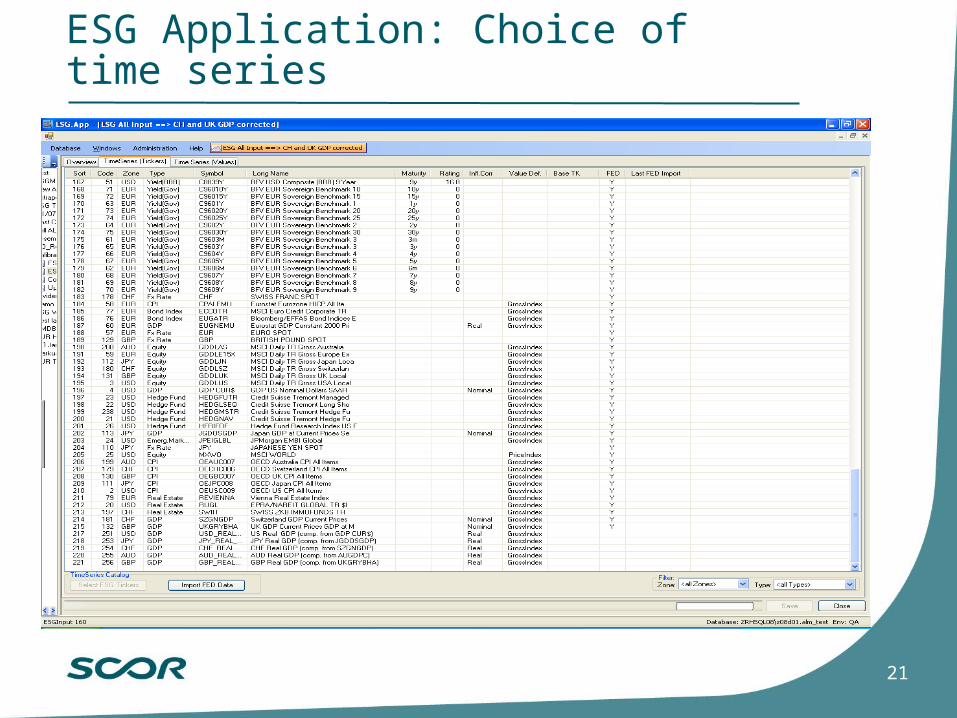
ESG Application: Choice of time series

22

ESG Application: Many time series values, analyzing completeness and correctness

23

Input data validation and completion in the ESG Application

~50 quarterly observations for hundreds of time series thousands of historical values to be validated, with regular addition of new data

Simple detection of suspicious values, identifying large deviations from expectation. Criterion: deviation > 4 times the standard deviation

Suspicious values have to be evaluated by human experts here

Eliminated bad values leave a data gap

Other data gaps originate from data sources (e.g.delayed reporting of inflation figures)

The method requires completeness of input data gap filling

Need data interpolation and extrapolation

univariate gap filling algorithms, using one time series only

multivariate gap filling, e.g. estimating missing yield values of one maturity based on yield values of other maturities

24

Result example: Simulated yield curves, simulation 2007Q3 end 2008

EUR yield curve (zero coupon, risk-free), Sep 2007 and examples of simulated curves for Dec 2008

2%

3%

4%

5%

6%

0 1 2 3 4 5 6 7 8 9 10 11 12 13 14 15 16 17 18 19 20

Maturity [years]

Inte

res

t ra

te le

ve

l

curve of 2007Q3

simulation example 1

EUR yield curve (zero coupon, risk-free), Sep 2007 and examples of simulated curves for Dec 2008

2%

3%

4%

5%

6%

0 1 2 3 4 5 6 7 8 9 10 11 12 13 14 15 16 17 18 19 20

Maturity [years]

Inte

res

t ra

te le

ve

l

curve of 2007Q3

simulation example 1

simulation example 2

EUR yield curve (zero coupon, risk-free), Sep 2007 and examples of simulated curves for Dec 2008

2%

3%

4%

5%

6%

0 1 2 3 4 5 6 7 8 9 10 11 12 13 14 15 16 17 18 19 20

Maturity [years]

Inte

res

t ra

te le

ve

l

curve of 2007Q3

simulation example 1

simulation example 2

simulation example 3

EUR yield curve (zero coupon, risk-free), Sep 2007 and examples of simulated curves for Dec 2008

2%

3%

4%

5%

6%

0 1 2 3 4 5 6 7 8 9 10 11 12 13 14 15 16 17 18 19 20

Maturity [years]

Inte

res

t ra

te le

ve

l

curve of 2007Q3

simulation example 1

simulation example 2

simulation example 3

simulation example 4

25

Case study 3: High-frequency ticker data

Tick-by-tick data, irregularly spaced, produced and collected in real time by banks, trading platforms or data vendors

Example: foreign exchange ticks, intra-day trading

Why to analyze such high-frequency data?

Measuring „Realized Volatility” with high precision

High-frequency, real-time risk assessment

Automated information services or trading algorithms

Research (pioneer work by Olsen & Associates in the 1990s)

Time series with huge numbers of observations: thousands per day, millions in years

Too many data for human validation and cleaning, need automated algorithms

26

Special requirements for the analysis and the filtering of high-frequency data

Returns of market prices often have distributions with heavy tails and fluctuating volatility levels problem: „outliers“ may be correct. Need to a good model of true behavior to identify wrong data

Real-time data cleaning is hard: decision on validity needed before the arrival of new confirming observations

Time matters: The first tick after a period of missing data is especially hard to validate

Validation is easier when shifts are rapidly confirmed by many new ticks

Introduce an adaptive filter that learns from the data while validating:

The cleaning algorithm carries its own statistics calculator

Data cleaning parameters continuously adapt to statistics

Algorithm survives shifts in market behavior, structural breaks

27

Conclusion: Recommended procedure for data cleaning

Data source 1 Data source 2

Evaluation of Outliers by

Human Experts Error

Identification

Sophisticated Statistical Criteria, Adaptive

Filtering Automatic Error

Detection

Validated Data Set, Possibly

with Data Gaps

Data Gap Filling (Intrapolation, Extrapolation),

if Required

Basic Historical Data Set

Simple Statistical

Outlier Analysis Suspicious

Data

Main Data Analysis: Robust

Methods if Possible (Hardly Possible in Risk

Assessment)

↓ ↓

↓ ↓

↓

↓

→ →

↑

28

Thank you …

... for your attention!