Section 1:

In the Parametric Method section of the course, we learned how to draw a separation hyperplane between two classes by obtaining w0, the argmax of the cost function J(w)=wTSBw / wTSww. The solution was found to be w0= Sw

-1(m1-m2), where m1 and m2 are the sample means of each class, respectively.

Some students raised the question: can one simply use J(w)= wTSBw instead (i.e. setting Sw as the identity matrix in the solution wo? Investigate this question by numerical experimentation.

In our numerical experiment, the data used is of the following nature: • We decided on using 3 class data • An 8 dimensional data was chosen to be reduced to a 3 –dimensional using fisher

linear discriminant analysis. o The choice of 8D data is arbitrary o It is reduced to 3-d because we have 3 classes and it is possible to

visualize the 3-d data • The data is a random sample from ‘Multivariate Normal Distribution’.

o We have used ‘mnvrnd’ from MATLAB to generate the data • The code for FLDA (Fisher Linear Discriminant Analysis) is obtained from

http://www.mit.edu/~linuo/Matlab%20Scripts.html • We have used 300 training data points and 150 test data points

We followed the “Design of Experiment” methodology to run our numerical experiments. The following two factors are considered here:

1. Mean of the normal distribution 2. Co-variance of the normal distribution 3. Co-variance taken as Identity Matrix

For each of the above factors we have a ‘high value’ and ‘low value’ as explained below:

1. Distribution means a. If the distribution means of the 3 classes are far apart we consider this as

the ‘high’ value else it is ‘low value’ 2. Co-Variance

a. The ‘covariance matrix elements’ of the distributions are taken either less than 1 (< 1) for small covariance case or >>1 (greater than 1 and less than 10) for large covariance case.

3. For the case of analyzing the importance of within class scatter, covariance is taken as an identity matrix (for low value) or as stated in point 2 (high value)

a. Scatter matrix is Identity Matrix – Low value b. Scatter matrix is not Identity Matrix but calculated – High value

We have a total of 8 (2 * 2 * 2) possible experiments. We have a repeat for each experiment to confirm the experimental run. We have performed the classification using majority voting procedure and the results are shown in Table 1:

High (Mean & Covariance)

Low (Mean & Covariance)

High Covariance & Low Mean

Low Covariance & High Mean

High (Scatter)

0.7 0.91 0.87 0.72 Low (Scatter)

0.67 0.9 0.73 0.67

Table 1. Classification Results of the test data reduced from 8-D space to 3-D space

Reasoning: We found that the scatter (with-in class) has to be minimized because a huge spread in the data points of the classes resulted in an inefficient classification (bolded in the table above). This is evident in the case where the means are not far apart and the covariance matrix of the classes is high (The spread is high). Minimizing the with-in class scatter has always resulted in a better classification as seen in the results above. The figures below help in visualizing the classification.

-40

-20

0

20

-1-0.500.511.5-8

-6

-4

-2

0

2

4

6

X-Axis

Data Projected onto 3-D space using Fisher-LDA (Calculated Scatter Matrix)

Y-Axis

Z-A

xis

Class-1Class-2Class-3

-1000

-500

0

500

-100-50050100150

-600

-400

-200

0

200

400

600

X-Axis

Data Projected onto 3-D space using Fisher-LDA(Scatter Matrix is an Identity Matrix)

Y-Axis

Z-A

xis

Class-1Class-2Class-3

Computational Issues & Conclusions: We have tested the computational issues that might arise for the calculation of the scatter matrix. As we increased the dimension (ex. >30) for a multi-class case (>2 classes), the computations became slow. We found that for a data-set with large number of features, the scatter matrix usage might result in a huge computational burden. The scatter matrix calculation plays an important role if the covariance matrix has large values resulting in correlation and large spread in the data. So we conclude that using the scatter matrix is a trade-off between the accuracy and computational burden. Section 2: Database Used for the Experiments: We have used Reuters-21758 database for text classification in our experiments (see http://www.cc.gatech.edu/~hskim/). Throughout the report, we assume that the document set is represented in an m x n (term x document) matrix. Each value in the matrix represents the normalized frequency of appearance of a term in a document. The basis for normalization is given in [1]. Data of only 10 classes is used for training and testing purposes as the computational complexity increased drastically with the number of classes. The number of terms used to identify the documents is 11941. We have used 712 documents for training and 274 documents for testing purposes. Hence, the size of training database is 11941 x 712, and the size of testing database is 11941 x 274.

Dimension Reduction: Since we are using only 10 classes of data, 11941 dimensions are redundant for classification. Hence we perform dimension reduction on the original database. Intuitively, since we have 10 classes, we have reduced the database to 10 dimensions. The dimension reduction is performed using the ‘Centroid Algorithm’ [1]. For achieving good results, we first cluster the data using k-means clustering algorithm and then reduce the dimensions of the database using the centroid algorithm. This preserves the clusters after dimension reduction also. Throughout this report we use the term ‘Reduced Data’ to refer to the data obtained by performing dimension reduction. The dimensions of the reduced data used for training are 10 x 712 and those used for testing are 10 x 274. 2a) Data Classification using Support Vector Machines: Support vector machines (SVMs) are a set of related supervised learning methods used for classification and regression. SVMs were originally developed to for two-group classification problems, but the same approach has been used for multiple classes [2, 3]. SVMs produce a quadratic programming (QP) problem. There exist different approaches to solve this problem namely all-together, one-against-one and one-against-all as mentioned in [2]. Hsu et al. presented a survey comparing these three techniques in [2], showing that ‘one-against-one’ technique produces better accuracy and requires less number of support vectors, and hence lower computation time. In our experiments we investigate this claim by classifying the reduced data using all the approaches and comparing the accuracy. We have implemented the three approaches on reduced data. Implementation: The MATLAB code is downloaded from http://asi.insa-rouen.fr/enseignants/~arakotom/toolbox/index.html. This code is explained in Section 4. Table 2a-1 shows the results of our experiments for ‘one-against-one’ approach comparing the accuracies of full data and reduced data. It can be seen that polynomial kernel results in the highest accuracy. It can also be seen that linear kernel performs better than Gaussian kernel. One of the possible reasons for this is that a linear kernel performs better than Gaussian kernel for Gaussian distributed data. The data used by us is approximately Gaussian; hence the linear kernel outperforms the Gaussian kernel. Table 2a-2 shows the comparison of accuracies obtained by various approaches. Note that these experiments are performed using the reduced data.

Kernel Training Accuracy (%) of Full Data

(11941 x 712)

Testing Accuracy (%) of Full Data

(11941 x 712)

Training Accuracy (%)

of Reduced Data (10 x 712)

Testing Accuracy (%)

of Reduced Data (10 x 712)

Linear (C = 1) 90.3 84.3 88.3 82.7 Linear (C= 10) 92.5 85.1 90.1 83.3 Poly (d = 2) 93.1 85.6 91.7 84.0 Poly (d = 3) 91.4 85.3 89.0 84.9

Poly (d = 4) 89.3 84.8 87.8 85.1 RBF (γ = 0.5) 92.0 85.6 89.2 82.9 RBF (γ = 1.0) 88.3 83.2 87.3 83.2 Gaussian 85.6 82.1 84.2 79.3 Table 2a-1. Accuracy measurements using ‘one-against-one’ approach in SVMs comparing the performance of classifier using full data and reduced data.

Kernel Scheme 1 Scheme 2 Scheme 3 Linear (C = 1) 82.7 80.7 79.1 Linear (C= 10) 83.3 83.3 81.2 Poly (d = 2) 84.0 83.5 82.0 Poly (d = 3) 84.9 84.2 83.3 Poly (d = 4) 85.1 84.2 82.1 RBF (γ = 0.5) 82.9 84.3 78.5 RBF (γ = 1.0) 83.2 83.1 79.6 Gaussian 79.3 78.7 77.5

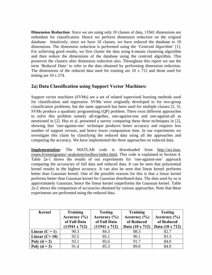
Table 2a-2. Comparison of testing accuracies for different approaches of solving QP in SVMs (Here scheme 1 is ‘one-against-one’, scheme 2 is ‘all-together’ and scheme 3 is ‘one-against-all’). Observation: We observe that there is a slight loss of accuracy by reducing the dimensions of the data, however by saving huge amount of computational time. The execution time of SVMs for full data requires more than 3 hrs, while the classification using reduced data takes few seconds. Also, from Table 2a-2, it is apparent that ‘one-against-one’ approach performs better than the other two approaches (‘one-against-all’ and ‘all-together’). This might not be true in all the cases. To play safe, it is better to use ‘all-together’ approach, which creates the decision boundary by considering all the classes. From our experiments, we can also see that the accuracies obtained by ‘one-against-one’ and ‘all-together’ approaches are almost the same. 2b) Data Classification using Artificial Neural Networks: Implementation: A MATLAB tool called ‘nntool’ is used for classifying the data using artificial neural networks. As can be seen from the Figure 2b-1, ‘nntool’ is a graphical user interface. The training data and the training class information can be either created or imported from the workspace. Since the Reuter’s data is huge, we have imported the ‘.mat’ files from the workspace. This tool facilitates us to select the type of neural network and the number of neurons.

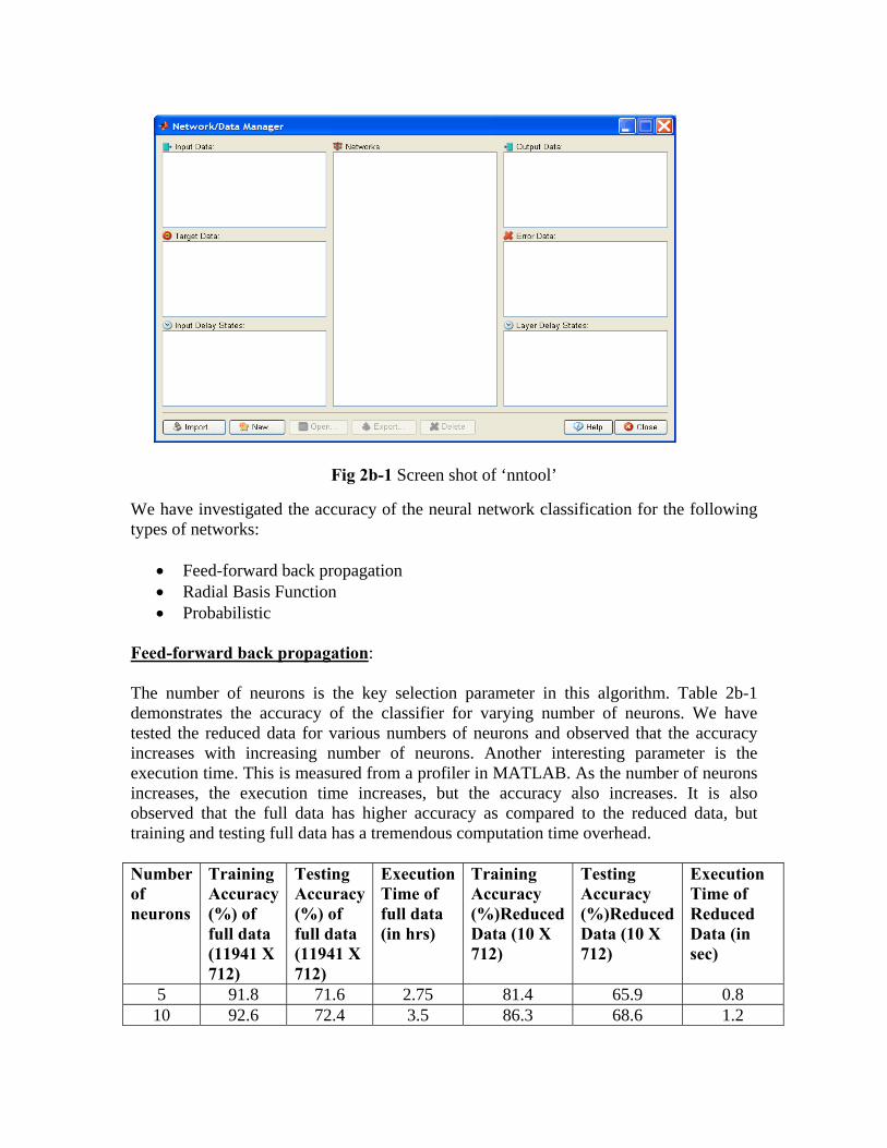
Fig 2b-1 Screen shot of ‘nntool’

We have investigated the accuracy of the neural network classification for the following types of networks:

• Feed-forward back propagation • Radial Basis Function • Probabilistic

Feed-forward back propagation: The number of neurons is the key selection parameter in this algorithm. Table 2b-1 demonstrates the accuracy of the classifier for varying number of neurons. We have tested the reduced data for various numbers of neurons and observed that the accuracy increases with increasing number of neurons. Another interesting parameter is the execution time. This is measured from a profiler in MATLAB. As the number of neurons increases, the execution time increases, but the accuracy also increases. It is also observed that the full data has higher accuracy as compared to the reduced data, but training and testing full data has a tremendous computation time overhead. Number of neurons

Training Accuracy (%) of full data (11941 X 712)

Testing Accuracy (%) of full data (11941 X 712)

Execution Time of full data (in hrs)

Training Accuracy (%)Reduced Data (10 X 712)

Testing Accuracy (%)Reduced Data (10 X 712)

Execution Time of Reduced Data (in sec)

5 91.8 71.6 2.75 81.4 65.9 0.8 10 92.6 72.4 3.5 86.3 68.6 1.2

20 > 5 hrs 91.2 69.1 1.8 30 95.8 72.5 2.4 40 96.4 75.3 3.2 50 97.2 78.6 5.8

Table 2b-1. Accuracy measurements using feed-forward back-propagation neural networks for varying number of neurons. (The empty boxes correspond to cases with very high execution time, these cases are omitted). Radial Basis Function: Literature survey says that neural networks with radial basis function achieve very high accuracy for most of the data sets [4]. So, it is important to compare other types of neural networks with that using radial basis function. There is a critical implementation issue arising with the representation of the class information in this case. The class information has to be represented in the form of a vector (of size #classes x #documents) each column containing all zeros except a one in the row corresponding to the class it belongs to, instead of a row/column vector. This helps in perceiving and building the network with a better accuracy. The second and the third columns of Table 2b-3 show this difference in accuracies. The testing accuracy obtained for the first case is 17.8%, where as the accuracy for the second case is 86.5%. Training Accuracy

(%) Testing Accuracy (%) Execution Time

Full Data (11941 X 712)

87.8 83.7 3.25 hrs

Reduced Data (10 X 712) (without converting the class info. to vectors)

91.6 17.8 2.7 sec

Reduced Data (10 X 712) (after converting the class info. to vectors)

99.1 86.5 2.7 sec

Table 2b-3. Accuracy and execution time measurements for neural networks using radial basis function We use a MATLAB command called ‘ind2vec’ to convert the row vector into a vector of size (#classes x #documents) Probabilistic Neural Networks:

Probabilistic neural networks are implemented by determining the density of the data using Parzen windows, and classifying them using the neural networks. Table 2b-2 shows the accuracy and execution time of the Reuter’s data. It cab be seen that huge amount of time (> 3hrs) can be saved by reducing the dimension, with only little loss in accuracy (1.5%). It is always not necessary that the dimension reduction causes loss of accuracy. Sometimes, the necessary information is lost; so the performance degrades. Sometimes, the dimension reduction can reduce the noise, thereby increasing the performance of the classifier. Since we are using cluster preserving technique, not much information is lost, so the accuracy does not vary significantly. Training Accuracy (%) Testing Accuracy (%) Execution Time Full Data (11941 X 712)

87.19 85.84 3.12 hrs

Reduced Data (10 X 712)

83.34 84.32 3.2 sec

Table 2b-2. Accuracy and execution time measurements for probabilistic neural networks Observation: By comparing the above three types of neural networks, we observed that neural networks implemented using radial basis functions have higher performance than other two types of networks for Reuter’s data. Also, dimension reduction does not result in loss of accuracy to a very great extent, but reduces the computation time by a great deal. 2c) Comparing SVMs and Artificial Neural Networks: Theoretical:

• Hidden neurons are the building blocks of the artificial neural networks where as support vectors are the building blocks of SVMs.

• Artificial neural networks can be used for regression where as SVMs cannot be.

Experimental: From the results of our experiments, we observe that:

• For the reduced data, we observe that the execution time of SVMs is less than that of ANNs to achieve comparable accuracy, though SVMs solve the quadratic programming problem. The possible explanation is that, in ANNs, the number of parameters (weights + bias) to be optimized is large (for 50 neurons in hidden layer, it is approximately 1000).

• In our experiments, the highest accuracy for SVMs is achieved by a polynomial kernel, where as the highest accuracy for ANNs is achieved by an RBF neuron.

Section 3: 3a) Data Classification Using Parzen Windows: Parzen window is used to estimate the density in a non-parametric fashion and build a classifier based on the densities of classes. The code downloaded from http://www.mathworks.com/matlabcentral/fileexchange/loadFile.do?objectId=11880&objectType=FILE is used for our experiments. The files used in our experiments are discussed in Section 4. This code determines the density of the sample data and uses this data to build a neural network classifier to classify the data. The parameter ‘spread’ determines the Parzen window (RBF spread in this code) size. The code uses a radial basis Parzen window (see http://www.faqs.org/faqs/ai-faq/neural-nets/part2/section-20.html) and varied the spread for varying the window size. Gaussian Parzen windows can also be used and the variance can be varied to vary the window size. Table 3a shows the training and testing accuracies for the full and reduced data using various spreads. From the results, it is apparent that accuracy degrades when the window size is too small or too large. This is because, smaller windows do not generalize the distribution, where as larger windows result in over-generalizing, thus degrading the accuracy. The underlined accuracies are the best accuracies obtained with the given parameters.

Spread Full Data Training

Accuracy (%) (11941 x 712)

Full Data Testing

Accuracy (%) (11941 x 712)

Reduced Data Training

Accuracy (%) (10 x 712)

Reduced Data Testing

Accuracy (%) (10 x 712)

0 3.2 8.7 0 7.3 0.05 97.3 78.9 94.5 76.7 0.1 91.2 77.3 89.33 77.370.15 87.9 75.2 85.39 74.45 0.2 85.6 74.3 82.87 70.07 0.5 61.2 52.1 58.15 45.99 1.0 41.0 32.4 35.96 29.2

Table 3a Comparison of accuracies for full and reduced data using various spreads of Parzen window. Note: It is observed that the MATLAB function ‘newpnn’ achieves the same results. This function also implements the density estimation and building a neural network classifier. 3b,c) Data Classification Using KNN: Brief introduction to the k-nearest neighbor algorithm

The k-nearest neighbor algorithm is a simple machine learning algorithm. An object is classified by a majority vote of its neighbors, with the object being assigned to the class most common amongst its k- nearest neighbors. k is a positive integer, typically small. If k = 1, then the object is simply assigned to the class of its nearest neighbor (called nearest neighbor algorithm). In binary (two class) classification problems, it is helpful to choose k to be an odd number as this avoids tied votes. Table 3bc shows the performance of the classifiers for varying number of neighbors. # Neighbors Type Euclidean Manhattan Cosine Correlation

Nearest 73.7 74.8 74.8 74.1 Random 73.7 74.8 74.8 74.1

1

Consensus 73.7 74.8 74.8 74.1 Nearest 73.36 75.55 76.3 76.64Random 74.1 75.2 77 75.91

5 Consensus 51.8 52.2 55.1 53.3

Nearest 74.45 74.81 75.18 75.55 Random 74.1 74.45 74.82 75.18

15 Consensus 33.2 33.9 40.14 40.15

Nearest 75.91 74.82 75.91 76.64 Random 76.3 74.82 75.91 76.3

30 Consensus 20.07 18.97 24.82 24.82

Nearest 75.55 76.3 73.732 72.99 Random 75.55 75.18 73.72 73

45 Consensus 10.95 8.03 17.52 18.25

Nearest 74.81 75.18 72.99 73.35 Random 74.45 74.45 73.36 73

60 Consensus 7.66 7.29 12.77 12.77

Nearest 73.36 71.17 70.44 68.98 Random 73.36 71.17 70.07 68.98

100

Consensus 0 0 3.28 0.73 Nearest 68.25 67.52 68.61 60.95 Random 67.52 66.79 67.88 60.95

150

Consensus 0 0 0 0 Table 3bc. Accuracy results obtained by varying parameters namely, the number of neighbors, distance metric and decision rule. Procedure In the case of testing k-nearest neighbor algorithm, we have performed experiments changing k (number of nearest neighbors), distance type (Euclidean, Manhattan, Cosine and Correlation) and rule to classify (Nearest, Random and Consensus). We have used Matlab’s “knnclassify” to perform our experiments.

Observations 1. For selecting k We observe that increasing k doesn’t always increase the accuracy. For the nearest neighbor case (k=1) we observe that though the classifier accuracy is not optimal, it is comparable with the highest classification accuracy. Optimal k value (and the classification accuracy) depends on factors like the number of classes under consideration, amount of data and its quality (number of data points/class and features representing the class density). In our experiment with 10 classes and 10 features (reduced space), we observe that k=30 is the optimal neighbor number. By increasing k (k>30), we found that the classification accuracy has decreased. This could be attributed to losing of (distinct) boundaries between classes. Though increasing k reduces the effect of noise, it could also affect the class boundary distinction resulting in reduced classifier accuracy. 2. Distance Type The following distance metrics are used for comparison:

• Euclidean: second order norm between two points • Manhattan: Sum of absolute differences (also called city block) • Cosine: One minus the cosine of the angle included between points (treated as

vectors) • Correlation: One minus the sample correlation between points (treated as vectors)

We observe that the type of distance used has little effect on classification accuracy. We implemented the k-nearest neighbor algorithm on dimensionally reduced data. As we know dimensional reduction reduces the correlation between features. We attribute the dimensional reduction to be the reason for unaffected classification accuracy with distance type. 3. Classification Rule The following classification rules are used:

• Nearest: Majority rule with nearest point tie-break • Random: Majority rule with random point tie-break • Consensus: points where the all the k nearest neighbors are not from the same

class, are not assigned to any class.

We observe that ‘Consensus’ has the least classifier accuracy. This is because ‘Consensus’ rule doesn’t associate a data point to any class in case of a tie. We also observe that the consensus classifier accuracy has reduced with increase of k value. This is expected if the data is equally represented from all the classes (Data points/class).The ‘nearest’ and ‘random’ classification rules result in similar accuracies.

3d) Comparing Parzen windows, NN and kNN: As a rule of thumb, nonparametric density estimation usually requires a large amount of training data to provide a good estimate of the true distribution of a data set. However, the most important factor that is often overlooked is not the amount of training data, but rather how well the training set represents the actual distribution of the data. Due to the accuracy of our classifiers, it appears that the features obtained after the dimension reduction are highly representative of the overall data distribution. It is very difficult to differentiate the three techniques, because the performances vary depending on the parameters and applications. We observe the following differences for our text classification data:

• The classifier performance is determined by the window size in the case of Parzen windows, where as the number of neighbors and the distance metric in the case of kNN. For NN, however the number of neighbors is fixed, and the only parameter that can be varied is the distance metric.

• From our results, we observe that the classifier accuracy is very sensitive to

window size (or RBF spread) in case of Parzen windows, where as the number of neighbors and distance metric do not vary the accuracy drastically. For kNN and NN, the consensus method results in very low accuracy.

• The classification rule does not change the performance of the classifier in the

case of nearest neighbors because, we consider only one neighbor, where as for kNN (k>1), the majority classification rule results in high accuracy.

References:

[1] H. Kim, P. Howland, and H. Park, Dimension Reduction in Text Classification with Support Vector Machines, Journal of Machine Learning, Vol. 6, pp. 37-53.

[2] C.-W. Hsu and C.-J.Lin, A comparison of Methods for Multi-class Support Vector Machines, IEEE Transactions on Neural Networks, vol. 13, pp. 415-425, 2002.

[3] J. Wetson and C. Watkins, Multi-class Support Vector Machines, Proceedings of ESANN99, Brussels, 1999. [4] Baughman, D. R. and Liu, Y. A. 1995 Neural Networks in Bioprocessing and Chemical Engineering: with Disk. 1st. Academic Press, Inc.

Section 4: MATLAB Code: The following code implements dimension reduction: % code for clustering the data % k-means clustering is implmented as its (see wikipedia) easy and k can be % mentioned before the start of clustering. %X is the data to be clustered % In our case k = 10 classes clc; clear; %X should be of the form documents * termmatrix for kmeans clustering %traindata is of the reqd form. % I am testing on 712 documents. So its 712 * 11941 matrix X = dlmread('traindata_1.txt'); %the loop below builds class information file. Each row is a document and the value of the class info file tells us which class it belongs to classData = dlmread('classdata_train.txt'); k=1; classInfo = zeros(max(classData),1); for i=1:1:length(classData) for j=k:1:classData(i) classInfo(j,1)=i; end k=classData(i)+1; end dlmwrite('classInfo.txt',classInfo'); %C is the cluster centroid matrix %if X is n*m then C is k*m where k is number of clusters % in our case n is the total number of documents (training) and k will be % reduced document clusters k=10; %[CI C] = kmeans(X,k); [CI C] = kmeans(X,k,'emptyaction','singleton');

%to get columns as clusters, we take transpose C=C'; dlmwrite('centroid_indeces.txt',CI); dlmwrite('centroid.txt',C); % below we will build a cluster class matrix for the clustered data cC = zeros(k,length(classData)); for i=1:1:length(classInfo) cC(CI(i,1),classInfo(i,1))= cC(CI(i,1),classInfo(i,1)) +1; end dlmwrite('cC.txt',cC); [Mcc Icc] = max(cC,[],2); dlmwrite('cCIndex.txt',Icc); %Icc1 tells us what clusters belong to what class %For dimensionality reduction case Training is done on the clustered data. %so we will do C = C' above %Dimensionality Reduction methods %1. Centroid Algorithm for Dimension Reduction s1 = size(X); %for all rows of X i.e for all documents for i=1:1:s1(1,1) redA1(:,i) = lsqnonneg(C,X(i,:)'); end %write the redA1 dlmwrite('redA1.txt',redA1); %X has dimension termmatrix * docs (11914 * 714) is reduced to (redA) with %10 * 714 % have to perform clustering on the reduced data!!!! We have to use the % same number of clusters as in the beginning. It is 10 in our case. redA1=redA1'; redA2=redA2';

k=10; [X1 C1] = kmeans(redA1,k,'emptyaction','singleton'); C1 = C1'; %in the case of training with dim. reduced clustered data, we have to use C1 %we have to build a 10 * 10 matrix for finding the class that each cluster %will belong to %k is the no of clusters k=10; clustClass1 = zeros(k,length(classData)); clustClass2 = zeros(k,length(classData)); for i=1:1:length(classInfo) clustClass1(X1(i,1),classInfo(i,1))= clustClass1(X1(i,1),classInfo(i,1)) +1; end dlmwrite('clustClass1.txt',clustClass1); [Mcc1 Icc1] = max(clustClass1,[],2); dlmwrite('ccIndex1.txt',Icc1); %Icc1 tells us what clusters belong to what class for i=1:1:length(classInfo) clustClass2(X2(i,1),classInfo(i,1))= clustClass2(X2(i,1),classInfo(i,1)) +1; end B1 = dlmread('testdata_1.txt'); s1=size(B1); for i=1:1:s1(1,1) redB1(:,i) = lsqnonneg(C,B1(i,:)'); end dlmwrite('test_data_centroid.txt',redB1); Prob 1)

• Matlab code for performing "Fisher linear discriminant" analysis was downloaded from http://mit.edu/~linuo/www/files/LDAplane.m

• This code takes the training data, its labels and test data as its arguments and returns the projected training and test data, projection plane details and the classification results.

MATLAB code: function [w, f, b, fTrain, fTest] = LDAplane (data, label, test) % Estimate the vector w normal to the linear discriminant hyperplane % data is the matrix: each row is one data point, each column is one % feature (dimension) of the data % % Note: currently, this program supports muliti classification, label has % to be adjcent integer numbers (e.g. [0 1 2 ...k] for k classes) % sorting matrix w=[]; f=[]; b=[]; fTrain=[]; fTest=[]; data=data'; featNum=size(data,1); dataNum=size(data,2); for Nclass=min(label):max(label) covB=[]; covW=[]; mui=[]; classLabel=(label==Nclass); for k=0:1 % Load digits x=data(:,find(classLabel==k)); eval(['x',num2str(k),'=x;']); %mean mui(:,end+1)=mean(x,2); end mu=mean(mui,2); %covariance covW=0; covB=0; for k=0:1 eval(['x=x',num2str(k),';']); for n=1:size(x,2) covW=covW+(x(:,n)-mui(:,k+1))*(x(:,n)-mui(:,k+1))'; end

end covW=covW/dataNum; %normal vector to Hyperplane classW=-inv(covW)*diff(mui,1,2); %offset prior=0; %prior=log(size(x0,2)/size(x1,2)); classB=1/2*sum(mui,2)'*inv(covW)*diff(mui,1,2)+prior; %projecting and offseting (this computes vote) fTestClass=-(test*classW+classB); fTrainClass=-(data'*classW+classB); %offseting classF=fTestClass; %Output into sorting matrix w(:,end+1)=classW; f(:,end+1)=classF; b(:,end+1)=classB; fTrain(:,end+1)=fTrainClass; fTest(:,end+1)=fTestClass; end % Classify by taking votes [dummy f]=max(f,[],2); f=f+min(label)-1; return

Prob 2)

a) The code for implementing support vector machines is downloaded from http://asi.insa-rouen.fr/enseignants/~arakotom/toolbox/index.html . We used the following functions for our experiments:

• svmmulticlass.m: function to determine the support vectors, given the

training data and the class information, using ‘all-together’ approach • svmmulticlassoneagainstone.m: function to determine the support vectors

using ‘one-against-one’ approach, given the training data and the class information.

• svmmulticlassoneagainstall.m: function to determine the support vectors using ‘one-against-all’ approach, given the training data and the class information.

• svmkernel.m: function to design the svm kernels used for training and classifying the data.

• svmmultival.m: function used to classify the data from the support vectors obtained from training.

b) Used ‘nntool’ and varied parameters (See the explanation in Section 2b for more

detail) svmmulticlass.m: function [xsup,w,b,nbsv,pos,alpha]=svmmulticlass(x,y,nbclass,C,epsilon,kernel,kerneloption,verbose, alphainit) % USAGE %[xsup,w,b,nbsv,pos,alpha]=svmmulticlass(x,y,nbclas,C,epsilon,kernel,kerneloption,verbose, alphainit) % % Support vector machine for multiclass CLASSIFICATION % This routine classify the training set with a support vector machine % using quadratic programming algorithm (active constraints method) % % INPUT % % Training set % x : input data % y : output data % parameters % c : Bound on the lagrangian multipliers % lambda : Conditioning parameter for QP method % kernel : kernel type. classical kernel are % % Name parameters % 'poly' polynomial degree % 'gaussian' gaussian standard deviation % % for more details see svmkernel % % kerneloption : parameters of kernel % % for more details see svmkernel % % verbose : display outputs (default value is 0: no display) % % alphainit : initialization vector of QP problem % % OUTPUT % % xsup coordinates of the Support Vector % w weight % b bias % pos position of Support Vector % alpha Lagragian multiplier

% % % see also svmreg, svmkernel, svmval if nargin< 9 alphainit=[]; end; if nargin < 8 verbose = 1; end if nargin < 7 kerneloption = 5; end if nargin < 6 kernel = 'gaussian'; end if nargin < 5 epsilon = 0.0000001; end if nargin < 4 C = 10000000; end verbose %------------------------------------------------------ % initialisation %------------------------------------------------------- [y,ind]=sort(y); x=x(ind,:); yextended=repmat(y,nbclass,1); xextended=repmat(x,nbclass,1); ell=size(x,1); n=sum(y==1); if size(C,1)==1 C=C*ones(size(y)); end; %------------------------------------------------------ % construction des matrices associé au pb QP %------------------------------------------------------- MatAux=zeros(ell,ell); MatAuxQ3=zeros(ell,ell); Q21=zeros(ell*nbclass,ell*nbclass); Q22=zeros(ell*nbclass,ell*nbclass);

debut=1; debutQ3=1; for s=1:nbclass indclass=find(y==s); ellinclass=length(indclass); MatAux(debut:debut+ellinclass-1,debut:debut+ellinclass-1)=svmkernel(x(indclass,:),kernel,kerneloption); debut=debut+ellinclass; MatAuxQ3(debutQ3:debutQ3+ell-1,debutQ3:debutQ3+ell-1)=svmkernel(x,kernel,kerneloption); debutQ3=debutQ3+ell; for j=1:ell Kij=svmkernel(x,kernel,kerneloption,x(j,:)); yj=y(j); Q21( (yj-1)*ell +1: yj *ell, (s-1)*ell + j )= -Kij; ind=find(yextended==s); Q22(ind,(s-1)*ell + j )= - svmkernel(xextended(ind,:),kernel,kerneloption,x(j,:)); end; end; Q1=repmat(MatAux,nbclass,nbclass); Q3=MatAuxQ3; Q2=Q21+Q22; Q=Q1+Q2+Q3; %------------------------------------------------------ % Les contraintes %------------------------------------------------------- yii=[]; Am=zeros(nbclass, size(yextended,1)); Am1=zeros(nbclass, size(yextended,1)); for s=1:nbclass ind=(s-1)*ell+1: s*ell; Am(s,ind)=ones(1,length(ind)); ind1=find(yextended==s); Am1(s,ind1)=ones(1,length(ind1)); yii= [yii;y==s]; end; A=Am-Am1; c=2*ones(size(yextended)); b=zeros(size(A,1),1); Cvect=repmat(C,3,1); unused=find(yii==1); Cvect(unused)=0.00000*ones(length(unused),1);

xinit=zeros(size(Cvect)); xinit(n+1)=Cvect(n+1)/2; [xnew, lambda, pos] = monqp(Q,c,A',b,Cvect,epsilon,verbose,x,[],xinit); b=-lambda; alpha=zeros(size(Cvect)); alpha(pos)=xnew; w=zeros(size(xextended,1),1); xsup=[]; for s=1:nbclass for i=1:ell if y(i)==s for m=1:nbclass w((s-1)*ell+i)=w((s-1)*ell+i)+alpha((m-1)*ell+i); end; end; w((s-1)*ell+i)=w((s-1)*ell+i)-alpha((s-1)*ell+i); end; end; waux=[]; for s=1:nbclass ind=find(w((s-1)*ell+1:(s-1)*ell+ell)~=0); waux=[waux;w( (s-1)*ell+ ind)]; nbsv(s)=length(ind); xsup=[xsup; x(ind,:)]; end; w=waux; svmmulticlassoneagainstall.m: function [xsup,w,b,nbsv,pos,obj]=svmmulticlassoneagainstall(x,y,nbclass,c,epsilon,kernel,kerneloption,verbose,warmstart); % USAGE [xsup,w,b,nbsv,pos,obj]=svmmulticlass(x,y,nbclass,c,epsilon,kernel,kerneloption,verbose); % % % SVM Multi Classes Classification One against Others algorithm % % y is the target vector which contains integer from 1 to nbclass. % % This subroutine use the svmclass function % % the differences lies in the output nbsv which is a vector % containing the number of support vector for each machine % learning. % For xsup, w, b, the output of each ML are concatenated % in line.

% % % See svmclass, svmmultival % xsup=[]; % 3D matrices can not be used as numebr of SV changes w=[]; b=[]; pos=[]; span=1; qpsize=1000; nbsv=zeros(1,nbclass); nbsuppvector=zeros(1,nbclass); obj=0; for i=1:nbclass yone=(y==i)+(y~=i)*-1; if exist('warmstart') & isfield(warmstart,'nbsv'); nbsvinit=cumsum([0 warmstart.nbsv]); alphainit=zeros(size(yone)); alphainit(warmstart.pos(nbsvinit(i)+1:nbsvinit(i+1)))= abs(warmstart.alpsup(nbsvinit(i)+1:nbsvinit(i+1))); else alphainit=[]; end; if size(yone,1)>4000 [xsupaux,waux,baux,posaux]=svmclassls(x,yone,c,epsilon,kernel,kerneloption,verbose,span,qpsize,alphainit); else [xsupaux,waux,baux,posaux,timeaux,alphaaux,objaux]=svmclass(x,yone,c,epsilon,kernel,kerneloption,verbose,span,alphainit); end; nbsv(i)=length(posaux); xsup=[xsup;xsupaux]; w=[w;waux]; b=[b;baux]; pos=[pos;posaux]; obj=obj+objaux; end; svmmulticlassoneagainstone.m: function [xsup,w,b,nbsv,classifier,pos,obj]=svmmulticlassoneagainstone(x,y,nbclass,c,epsilon,kernel,kerneloption,verbose,warmstart); %[xsup,w,b,nbsv,classifier,posSigma]=svmmulticlassoneagainstone(x,y,nbclass,c,epsilon,kernel,kerneloption,verbose); % % %

% SVM Multi Classes Classification One against Others algorithm % % y is the target vector which contains integer from 1 to nbclass. % % This subroutine use the svmclass function % % the differences lies in the output nbsv which is a vector % containing the number of support vector for each machine % learning. % For xsup, w, b, the output of each ML are concatenated % in line. % % classifier gives which class against which one % if nargin < 8 verbose=0; end; xsup=[]; % 3D matrices can not be used as numebr of SV changes w=[]; b=[]; pos=[]; SigmaOut=[]; span=1; classifier=[]; nbsv=zeros(1,nbclass); nbsuppvector=zeros(1,nbclass); k=1; if isempty(x) & strcmp(kernel,'numerical') & isfield(kerneloption,'matrix') Kaux=kerneloption.matrix; kernelparam=1; xapp=[]; else kernelparam=0; end; obj=0; for i=1:nbclass-1 for j=i+1:nbclass indi=find(y==i); indj=find(y==j); yone=[ones(length(indi),1);-ones(length(indj),1)]; if ~isempty(x) xapp=[x(indi,:); x(indj,:)]; end; if exist('warmstart') & isfield(warmstart,'nbsv'); nbsvinit=cumsum([0 warmstart.nbsv]); alphainit=zeros(size(yone)); aux=[indi;indj]; posaux=find(ismember(aux,warmstart.pos(nbsvinit(k)+1:nbsvinit(k+1)))); alphainit(posaux)= abs(warmstart.alpsup(nbsvinit(k)+1:nbsvinit(k+1))); else alphainit=[];

end; if kernelparam==1; if size(indi,1)==1 && size(indi,2)>1 kerneloption.matrix=Kaux([indi indj],[indi indj]); else kerneloption.matrix=Kaux([indi ;indj],[indi; indj]); end end; [xsupaux,waux,baux,posaux,timeaux,alphaaux,objaux]=svmclass(xapp,yone,c,epsilon,kernel,kerneloption,verbose,span,alphainit); [n1,n2]=size(waux); nbsv(k)=n1; classifier(k,:)=[i j]; xsup=[xsup;xsupaux]; w=[w;waux]; b=[b;baux]; aux=[indi;indj]; pos=[pos;aux(posaux)]; obj=obj+objaux; k=k+1; end; end; svmkernel.m: function [K,option]=svmkernel(x,kernel,kerneloption,xsup,framematrix,vector,dual); % Usage K=svkernel(x,kernel,kerneloption,xsup,frame,vector,dual); % % Returns the scalar product of the vectors x by using the % mapping defined by the kernel function or x and xsup % if the matrix xsup is defined % % Input % % x :input vectors % kernel : kernel function % Type Function Option % Polynomial 'poly' Degree (<x,xsup>+1)^d % Homogeneous polynomial 'polyhomog' Degree <x,xsup>^d % Gaussian 'gaussian' Bandwidth % Heavy Tailed RBF 'htrbf' [a,b] %see Chappelle 1999 % Mexican 1D Wavelet 'wavelet' % Frame kernel 'frame' 'sin','numerical'... %

% kerneloption : scalar or vector containing the option for the kernel % 'gaussian' : scalar gamma is identical for all coordinates % otherwise is a vector of length equal to the number of % coordinate % % % 'poly' : kerneloption is a scalar given the degree of the polynomial % or is a vector which first element is the degree of the polynomial % and other elements gives the bandwidth of each dimension. % thus the vector is of size n+1 where n is the dimension of the problem. % % % xsup : support vector % % ----- 1D Frame Kernel -------------------------- % % framematrix frame elements for frame kernel % vector sampling position of frame elements % dual dual frame % frame,vector and dual are respectively the matrices and the vector where the frame % elements have been processed. these parameters are used only in case % % % see also svmreg,svmclass,svmval, kernelwavelet,kernelframe if nargin < 6 vector=[]; dual=[]; end; if nargin <5 frame=[]; end; if nargin<4 xsup=x; end; if nargin<3 kerneloption=1; end; if nargin<2 kernel='gaussian'; end; if isempty(xsup) xsup=x; end; [n1 n2]=size(x); [n n3]=size(xsup); ps = zeros(n1,n); % produit scalaire switch lower(kernel) case 'poly' [nk,nk2]=size(kerneloption); if nk>nk2

kerneloption=kerneloption'; nk2=nk; end; if nk2==1 degree=kerneloption; var=ones(1,n2); elseif nk2 ==2 degree=kerneloption(1); var=ones(1,n2)*kerneloption(2); elseif nk2== n2+1 degree=kerneloption(1); var=kerneloption(2:n2+1); elseif nk2 ==n2+2 degree=kerneloption(1); var=kerneloption(2:n2+1); end; if nk2==1 aux=1; else aux=repmat(var,n,1); end; ps= x *(xsup.*aux.^2)'; if degree > 1 K =(ps+1).^degree; else K=ps; end; case 'polyhomog' [nk,nk2]=size(kerneloption); if nk>nk2 kerneloption=kerneloption'; nk2=nk; end; if nk2==1 degree=kerneloption; var=ones(1,n2); else if nk2 ~=n2+1 degree=kerneloption(1); var=ones(1,n2)*kerneloption(2); else degree=kerneloption(1); var=kerneloption(2:nk2); end; end; aux=repmat(var,n,1); ps= x *(xsup.*aux.^2)'; K =(ps).^degree;

case 'gaussian' [nk,nk2]=size(kerneloption); if nk ~=nk2 if nk>nk2 kerneloption=kerneloption'; end; else kerneloption=ones(1,n2)*kerneloption; end; if length(kerneloption)~=n2 & length(kerneloption)~=n2+1 error('Number of kerneloption is not compatible with data...'); end; metric = diag(1./kerneloption.^2); ps = x*metric*xsup'; [nps,pps]=size(ps); normx = sum(x.^2*metric,2); normxsup = sum(xsup.^2*metric,2); ps = -2*ps + repmat(normx,1,pps) + repmat(normxsup',nps,1) ; K = exp(-ps/2); case 'htrbf' % heavy tailed RBF %see Chappelle Paper% b=kerneloption(2); a=kerneloption(1); for i=1:n ps(:,i) = sum( abs((x.^a - ones(n1,1)*xsup(i,:).^a)).^b ,2); end; K = exp(-ps); case 'gaussianslow' % %b=kerneloption(2); %a=kerneloption(1); for i=1:n ps(:,i) = sum( abs((x - ones(n1,1)*xsup(i,:))).^2 ,2)./kerneloption.^2/2; end; K = exp(-ps); case 'multiquadric' metric = diag(1./kerneloption); ps = x*metric*xsup'; [nps,pps]=size(ps); normx = sum(x.^2*metric,2); normxsup = sum(xsup.^2*metric,2); ps = -2*ps + repmat(normx,1,pps) + repmat(normxsup',nps,1) ; K=sqrt(ps + 0.1); case 'wavelet' K=kernelwavelet(x,kerneloption,xsup);

case 'frame' K=kernelframe(x,kerneloption,xsup,framematrix,vector,dual); case 'wavelet2d' K=wav2dkernelint(x,xsup,kerneloption); case 'radialwavelet2d' K=radialwavkernel(x,xsup); case 'tensorwavkernel' [K,option]=tensorwavkernel(x,xsup,kerneloption); case 'numerical' K=kerneloption.matrix; case 'polymetric' K=x*kerneloption.metric*xsup'; case 'jcb' K=x*xsup'; end; svmmultival.m: function [ypred,maxi,ypredMat]=svmmultival(x,xsup,w,b,nbsv,kernel,kerneloption) % USAGE ypred=svmmultival(x,xsup,w,b,nbsv,kernel,kerneloption) % % Process the class of a new point x of a one-against-all % or a all data at once MultiClass SVM % % This function should be used in conjuction with the output of % svmmulticlass. % % % See also svmmulticlass, svmval % [n1,n2]=size(x); nbclass=length(nbsv); y=zeros(n1,nbclass); nbsv=[0 nbsv]; aux=cumsum(nbsv); for i=1:nbclass if ~isempty(xsup) xsupaux=xsup(aux(i)+1:aux(i)+nbsv(i+1),:); waux=w(aux(i)+1:aux(i)+nbsv(i+1)); baux=b(i); ypred(:,i)= svmval(x,xsupaux,waux,baux,kernel,kerneloption); else if isempty(x) % Kernel matrix is given as a parameter waux=w(aux(i)+1:aux(i)+nbsv(i+1)); baux=b(i); kernel='numerical'; xsupaux=[]; pos=aux(i)+1:aux(i)+nbsv(i+1); kerneloption2.matrix=kerneloption.matrix(:,pos);

ypred(:,i)= svmval(x,xsupaux,waux,baux,kernel,kerneloption2); end; end; end; ypredMat=ypred; [maxi,ypred]=max(ypred'); maxi=maxi'; ypred=ypred'; Prob 3)

a) The MATLAB code is developed based on the code taken from http://www.mathworks.com/matlabcentral/ fileexchange/loadFile.do?objectId=11880&objectType=FILE . The following files are used for the classification:

• parzenPNNlearn.m – builds the neural network parameters from the densities of training data estimated by Parzen windows.

• parzenPNNclassify.m – classifies the test data based on the network parameters determined by the parzenPNNlearn.m

Alternately, the MATLAB function ‘newpnn’ can be used.

b, c) The MATLAB function ‘knnclassify’ is used to classify the data using k-Nearest Neighbors density estimation. k = 1 corresponds the ‘Nearest Neighbor’ classification.

parzenPNNlearn.m:

function net = parzenPNNlearn(samples,classification, spread) % PARZENPNNLEARN Creates a Parzen probabilistic neural network % % This funcion generates a Parzen PNN (Probabilistic Neural Network) from % a list of classified samples. The samples are given in the format of a % matrix containing a single sample per row. The returned structure is a % Parzen PNN and must be used with the parzen PNN manipulation functions. % % Parameters % ---------- % IN: % samples = The set of samples. % classification = The classification of the samples. % spread = Radial basis spread of the Parzen window % autocentering or not, whilst a vector can define the % selected center. (def=true) % OUT:

% net = The parzen PNN. % % Pre % --- % - The input samples must be passed as a row-samples matrix. % - The classification vector must have the same number of elements as the % number of columns of the samples matrix. % % Post % ---- % - The returned structure is a valid parzenPNN structure. % % Examples % -------- % % A training set for the class 'a' and 'b': % img=ones(100); % f=figure; imshow(img); sa=getpoints; close(f); % f=figure; imshow(img); sb=getpoints; close(f); % % The samples matrix: % S = [sa,sb]; % % The classification vector: % C = [repmat('a',[1,size(sa,2)]),repmat('b',[1,size(sb,2)])]; % % Generating the network: % net = parzenPNNlearn(S,C), % % See also % -------- % parzenPNNclassify, parzenPNNimprove % Check params: if nargin<2 || size(samples,2)~=numel(classification) error('A samples matrix and a classification vector must be provided!'); end if nargin<3 center=true; end % Generating the center: if isa(center,'logical') % Generating automatically the center: if center center = mean(samples,2); else center = zeros(size(samples,1),1); end else % Checking the given mean: if ~vectCheckShape(center,[size(samples,1),1]) error('The specified center is not a point of the samples space (wrong dimensionality)!'); end end % Counting the classes and generating the classes vector: classes = unique(classification);

% Centering the data: samples = samples - repmat(center,[1,size(samples,2)]); % Obtaining the normalization factors: normvals = sqrt(sum(samples.^2)); % Normalizing: samples = samples./repmat(normvals,[size(samples,1),1]); % Creating the network structure: net.ws = samples; net.classes = classes; net.center = center; % Preparing the set of classification indexes: nc = numel(classes); net.classInds = cell(1,nc); for i=1:nc % Finding the indexes for this class: net.classInds{i} = find(classification==classes(i)); end net.b{1} = zeros(Q,1)+sqrt(-log(.5))/spread;

parzenPNNclassify.m:

function [class,score,scores] = parzenPNNclassify(net,X,nonlin) % PARZENPNNCLASSIFY Classifies a vector x given a parzenPNN network. % % This funcion uses a Parzen PNN (Probabilistic Neural Network) to % classify a given vector x. Also the scores of the vector are given to % allow to the user to manipulate it and compute confidences. % % Parameters % ---------- % IN: % net = The parzen PNN. % X = The matrix containing column vectors that must be classified. % nonlin = The nonlinearity funciton or the sigma value for the default % one. (def=@(u)(exp((u-1)./sigma.^2))) (def sigma=2) % OUT: % class = The class of the vector. % score = The score of the selected class. % scores = The scores obtained for each class. % % Pre % --- % - The input network must be a valid parzenPNN structure. % - The vector x must have the same number of elements as the % number of columns of the samples matrix in the network. % % Post % ----

% - Only a class is returned. % - A score is returned in the vector scores for each class. % % Check params: if nargin<2 || size(net.ws,1)~=size(X,1) error('A valid parzenPNN and a vector with the same number of values must be provided!'); end if nargin<3 % A nonlinearity with default sigma: nonlin = @(u)(exp((u-1)./4)); elseif ~isa(nonlin,'function_handle') % Using nonlin as the sigma value: sigma = nonlin; nonlin = @(u)(exp((u-1)./sigma.^2)); end % Centering the data: X = X - repmat(net.center,[1,size(X,2)]); % Compute the activation values for the first nurons layer: activations = X'*net.ws; % Using the nonlinearity function: activations = nonlin(activations); % Generating the scores: nc = numel(net.classes); nx = size(X,2); scores = zeros(nx,nc); for i=1:nc % Getting the activation values for this class and summing up: scores(:,i) = sum(activations(:,net.classInds{i}),2); end % Selecting the winning class: class = repmat(net.classes(1),[1,nx]); score = zeros(1,nx); for j=1:nx % Getting the best choice: [s,pos] = max(scores(j,:)); % Saving the values: score(j) = s; class(j) = net.classes(pos); end