Embed Size (px)
Citation preview

Data Break 7: Kriging the Meuse River
BIOS 737 Fall 2012
Fall 2012
BIOS 737 Data Break 7: Kriging the Meuse River
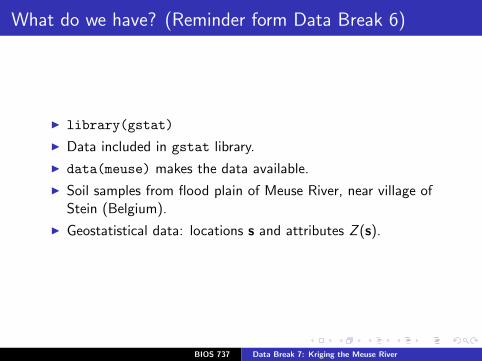
What do we have? (Reminder form Data Break 6)
I library(gstat)
I Data included in gstat library.
I data(meuse) makes the data available.
I Soil samples from flood plain of Meuse River, near village ofStein (Belgium).
I Geostatistical data: locations s and attributes Z (s).
BIOS 737 Data Break 7: Kriging the Meuse River

What do we want?
I Predictions of zinc across the entire flood plain.
I Mean square prediction error at each point.
BIOS 737 Data Break 7: Kriging the Meuse River
Kriging steps
I Empirical semivariogram.
I Fit theoretical semivariogram to empirical semivariogramvalues.
I Krige with best fitting semivariogram values.
BIOS 737 Data Break 7: Kriging the Meuse River
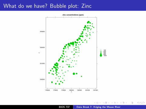
What do we have? Bubble plot: Zinc
zinc concentrations (ppm)
x
y
330000
331000
332000
333000
178500 179000 179500 180000 180500 181000 181500
1002004008001600
BIOS 737 Data Break 7: Kriging the Meuse River
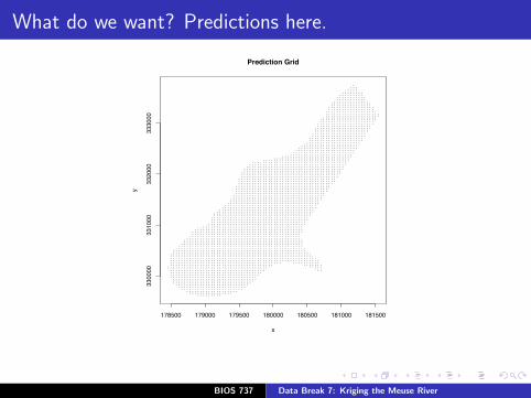
What do we want? Predictions here.
178500 179000 179500 180000 180500 181000 181500
330000
331000
332000
333000
x
y
Prediction Grid
BIOS 737 Data Break 7: Kriging the Meuse River
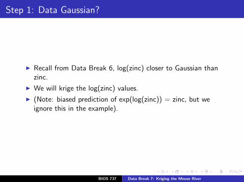
Step 1: Data Gaussian?
I Recall from Data Break 6, log(zinc) closer to Gaussian thanzinc.
I We will krige the log(zinc) values.
I (Note: biased prediction of exp(log(zinc)) = zinc, but weignore this in the example).
BIOS 737 Data Break 7: Kriging the Meuse River
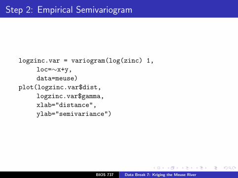
Step 2: Empirical Semivariogram
logzinc.var = variogram(log(zinc) 1,loc=∼x+y,data=meuse)
plot(logzinc.var$dist,logzinc.var$gamma,xlab="distance",ylab="semivariance")
BIOS 737 Data Break 7: Kriging the Meuse River
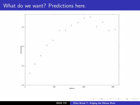
What do we want? Predictions here.
distance
semiva
riance
0.0
0.2
0.4
0.6
0 500 1000 1500
BIOS 737 Data Break 7: Kriging the Meuse River
Some other cool plots
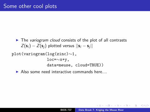
I The variogram cloud consists of the plot of all contrastsZ (si )− Z (sj) plotted versus ||si − sj ||
plot(variogram(log(zinc)∼1,loc=∼x+y,data=meuse, cloud=TRUE))
I Also some need interactive commands here....
BIOS 737 Data Break 7: Kriging the Meuse River
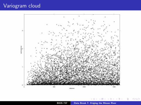
Variogram cloud
distance
semiva
riance
0
1
2
3
0 500 1000 1500
BIOS 737 Data Break 7: Kriging the Meuse River

Step 2: Fit Theoretical Semivariograms
I fit.variogram function in gstat
I Not entirely clear what optimization rule, based on practicalexperience rather than theoretical motivation.
I To get best fitting spherical semivariogram...
model.1 = fit.variogram(logzinc.var,vgm(psill=1,model="Sph",range=300,nugget=1))
plot(logzinc.var, model=model.1)title("Best Fit Spherical")
BIOS 737 Data Break 7: Kriging the Meuse River
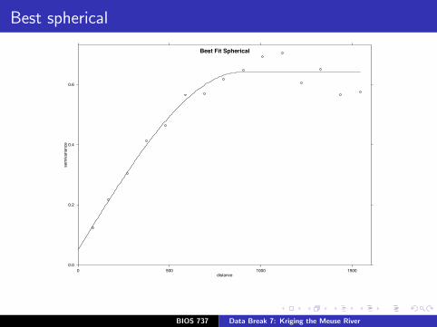
Best spherical
distance
semiva
riance
0.0
0.2
0.4
0.6
0 500 1000 1500
Best Fit Spherical
BIOS 737 Data Break 7: Kriging the Meuse River
Step 2: Fit Theoretical Semivariograms
I To get best fitting exponential semivariogram...
model.1 <- fit.variogram(logzinc.var,vgm(psill=1,model="Exp",range=300,nugget=1))
plot(logzinc.var, model=model.1)title("Best Fit Exponential")
BIOS 737 Data Break 7: Kriging the Meuse River
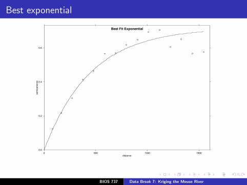
Best exponential
distance
semiva
riance
0.0
0.2
0.4
0.6
0 500 1000 1500
Best Fit Exponential
BIOS 737 Data Break 7: Kriging the Meuse River
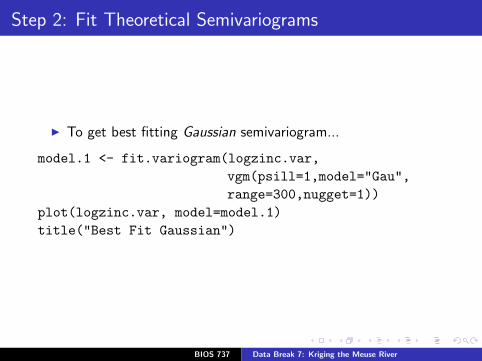
Step 2: Fit Theoretical Semivariograms
I To get best fitting Gaussian semivariogram...
model.1 <- fit.variogram(logzinc.var,vgm(psill=1,model="Gau",range=300,nugget=1))
plot(logzinc.var, model=model.1)title("Best Fit Gaussian")
BIOS 737 Data Break 7: Kriging the Meuse River

Best Gaussian
distance
semiva
riance
0.0
0.2
0.4
0.6
0 500 1000 1500
Best Fit Gaussian
BIOS 737 Data Break 7: Kriging the Meuse River
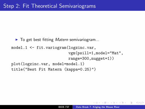
Step 2: Fit Theoretical Semivariograms
I To get best fitting Matern semivariogram...
model.1 <- fit.variogram(logzinc.var,vgm(psill=1,model="Mat",range=300,nugget=1))
plot(logzinc.var, model=model.1)title("Best Fit Matern (kappa=0.25)")
BIOS 737 Data Break 7: Kriging the Meuse River
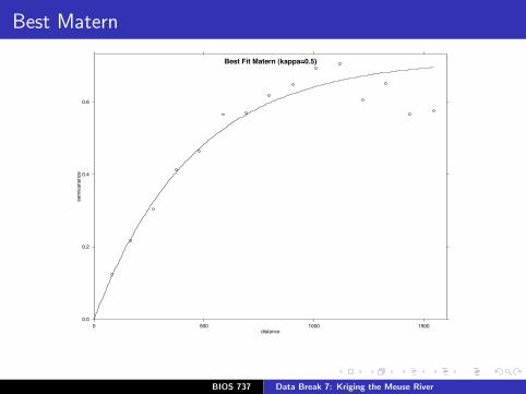
Best Matern
distance
semiva
riance
0.0
0.2
0.4
0.6
0 500 1000 1500
Best Fit Matern (kappa=0.5)
BIOS 737 Data Break 7: Kriging the Meuse River
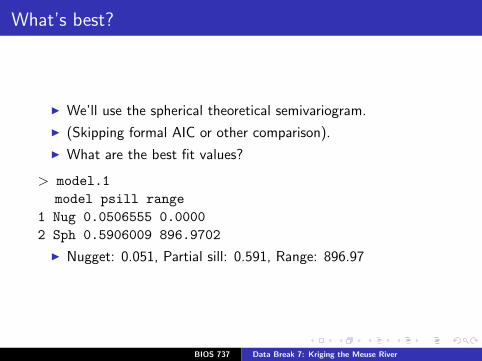
What’s best?
I We’ll use the spherical theoretical semivariogram.
I (Skipping formal AIC or other comparison).
I What are the best fit values?
> model.1model psill range
1 Nug 0.0506555 0.00002 Sph 0.5906009 896.9702
I Nugget: 0.051, Partial sill: 0.591, Range: 896.97
BIOS 737 Data Break 7: Kriging the Meuse River
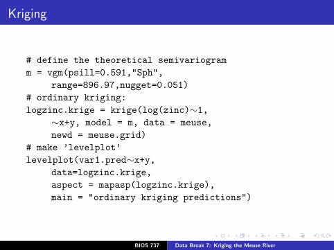
Kriging
# define the theoretical semivariogramm = vgm(psill=0.591,"Sph",
range=896.97,nugget=0.051)# ordinary kriging:logzinc.krige = krige(log(zinc)∼1,
∼x+y, model = m, data = meuse,newd = meuse.grid)
# make ’levelplot’levelplot(var1.pred∼x+y,
data=logzinc.krige,aspect = mapasp(logzinc.krige),main = "ordinary kriging predictions")
BIOS 737 Data Break 7: Kriging the Meuse River
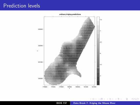
Prediction levels
ordinary kriging predictions
x
y
330000
331000
332000
333000
178500 179000 179500 180000 180500 181000 181500
−5
−5.5
−6
−6.5
−7
−7.5
BIOS 737 Data Break 7: Kriging the Meuse River
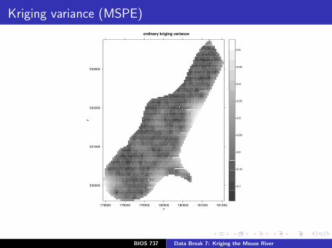
Kriging variance (MSPE)
ordinary kriging variance
x
y
330000
331000
332000
333000
178500 179000 179500 180000 180500 181000 181500
−0.1
−0.15
−0.2
−0.25
−0.3
−0.35
−0.4
−0.45
−0.5
BIOS 737 Data Break 7: Kriging the Meuse River
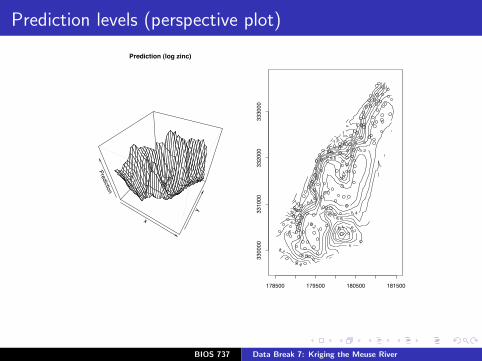
Prediction levels (perspective plot)
x
y
Prediction
Prediction (log zinc)
178500 179500 180500 181500
330000
331000
332000
333000
BIOS 737 Data Break 7: Kriging the Meuse River
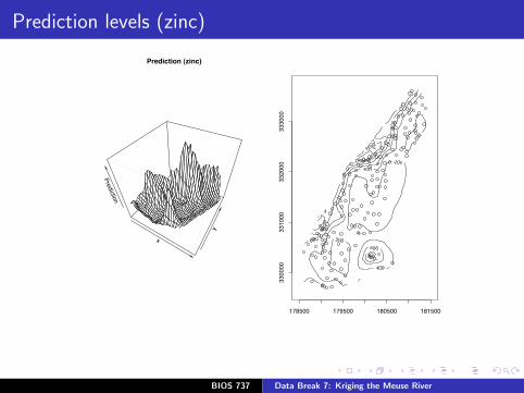
Prediction levels (zinc)
x
y
Prediction
Prediction (zinc)
178500 179500 180500 181500
330000
331000
332000
333000
BIOS 737 Data Break 7: Kriging the Meuse River
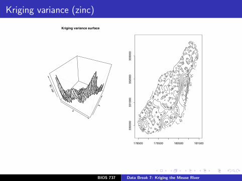
Kriging variance (zinc)
x
y
Kr. var
Kriging variance surface
178500 179500 180500 181500
3300
0033
1000
3320
0033
3000
BIOS 737 Data Break 7: Kriging the Meuse River
Notes
I MSPE highest where fewest observations.
I Back-transforming to original zinc levels gives idea ofprediction, but is no longer BLUP (we lose “L” and “U”).
I gstat does much more complicated analyses too.
BIOS 737 Data Break 7: Kriging the Meuse River
Summary of geostatistical methods
I We’ve really only seen the whirlwind tour of the basicelements.
I Semivariogram.
I Ordinary kriging.
I Many other options too.
I Questions?
BIOS 737 Data Break 7: Kriging the Meuse River
HW 3
I Repeat this analysis for the Smoky Mountain pH data.
I Should be able to use the data break code to do this.
I Due 12/3, graphs, output.
BIOS 737 Data Break 7: Kriging the Meuse River

Project 2
I Write up results of HW 4 as a report with Introduction,Methods, Results, and Discussion sections.
I Due 12/10, 5pm.
BIOS 737 Data Break 7: Kriging the Meuse River

![À } o © ] } } v Ì ] v · Bb7 Bb7 Db7 Db7 Eb7 Gm7 Db7 * D.C. al Fine Fine (third time) Db 13 Plav through entire form 3 ti mes. Db7 Eb7 F#m7](https://img.pdfslide.us/doc/110x75/5fbec29cae3b4c7bca046993/-o-v-oe-v-bb7-bb7-db7-db7-eb7-gm7-db7-dc-al-fine-fine-third.jpg)