Data-based Techniques to Improve State Estimation in Model …jbr · stay away from home for so long. My brother, Subash Rajaa, has been a constant source My brother, Subash Rajaa,

Data-based Techniques to Improve State Estimation in

Model Predictive Control

by

Murali Rajaa Rajamani

A dissertation submitted in partial fulfillment

of the requirements for the degree of

DOCTOR OF PHILOSOPHY

(Chemical Engineering)

at the

UNIVERSITY OF WISCONSIN–MADISON

2007

c© Copyright by Murali Rajaa Rajamani 2007

All Rights Reserved

i

To my family:

Dearest Dad, Mom, Brother and Paati

for their endless love and unconditional support

ii

Data-based Techniques to Improve State Estimation in

Model Predictive Control


Under the supervision of Professor James B. Rawlings

At the University of Wisconsin–Madison

Specifying the state estimator in model predictive control (MPC) requires sepa-

rate knowledge of the disturbances entering the states and the measurements, which

is usually lacking. In this dissertation, we develop the Autocovariance Least-Squares

(ALS) technique which uses the correlations between routine operating data to form a

least-squares problem to estimate the covariances for the disturbances. The ALS tech-

nique guarantees positive semidefinite covariance estimates by solving a semidefinite

programming (SDP) problem. Many efficient algorithms for solving SDPs are available in

the literature. New and simple necessary and sufficient conditions for the uniqueness of

the covariance estimates are presented. We also formulate the optimal weighting to be

used in the least-squares objective in the ALS technique to ensure minimum variance in

the estimates. A modification to the above technique is then presented to estimate the

iii

stochastic disturbance structure and the minimum number of disturbances required to

represent the data.

Simplifications to the ALS technique are presented to facilitate implementation. It

is also shown that the choice of the disturbance model in MPC does not affect the closed-

loop performance if appropriate covariances are used in specifying the state estimator.

The ALS technique is used to estimate the appropriate covariances regardless of the

plant’s true unknown disturbance source and the resulting estimator gain is shown to

compensate for an incorrect choice of the source of the disturbance.

The parallels between the ALS technique and the maximum likelihood estimation

(MLE) technique are shown by formulating the MLE as an equivalent ALS optimization

with a particular choice for the weighting in the ALS objective.

An industrial application of the ALS technique on a nonlinear blending drum

model and industrial operating data is described and the results are shown to give

improved state estimates as compared to rough industrial estimates for the covariances.

Moving horizon estimator (MHE) and particle filters (PF) are two common state

estimators used with nonlinear models. We present a novel hybrid of the MHE with the

PF to combine the advantages of both techniques. The improved performance of the

hybrid MHE/PF technique is illustrated on an example.

iv

v

Acknowledgments

I thank the Divine for giving me everything I have so far and for having blessed me with

good fortune. I am indebted to a great many people for making my years in Madison

and graduate school a priceless experience.

I begin with the following Sanskrit saying by Adi Shankara: “ Guru Brahma, Guru

Vishnu, Guru Devo Maheshwara. Guru Sakshath Parambrahma, Tasmai Shri Gurave

Namaha,” translated in English as “Guru is the creator Brahma, Guru is the preserver

Vishnu, Guru is the destroyer Shiva. Guru is directly the supreme spirit – I offer my

salutations to this Guru.” I consider my advisor Prof. Jim Rawlings to be my Guru,

without whose guidance I would not have gained even the fraction of my achievements

in Madison. I am amazed time and again by his clarity of thinking, depth of analysis

and simplification to the fundamentals. I will miss my intellectual interactions with him

and I hope I have another opportunity to work with him in the future. He has been an

idol to me and I will strive to think and work as efficiently and quickly as he.

I thank Profs. Graham, Maravelias, Barmish and Wright for taking time to be on

my thesis committee.

I reserve my deepest gratitude and love for my father. It was my Dad’s wish that

vi

I pursue my graduate studies in the USA, and is the only reason for my present stature.

His efforts and support for our family will remain unparalleled and I often look to the

heavens to seek his blessings. My mom has constantly showered me with affection and

reduced the physical distance between us through her love, making it possible for me to

stay away from home for so long. My brother, Subash Rajaa, has been a constant source

of encouragement and advice throughout my graduate school. Without his comfort,

love and words of wisdom my work here would have been impossible.

Mary Diaz has been the ‘mother’ to the Rawlings’ group and I have been especially

close to her. I will miss Mary and her goodies. John Eaton has been extremely helpful and

patient in answering all my dumb Linux questions. Within the Rawlings’ group, I have

developed friendships and acquaintances with past and present members. I treasure

my friendship with Paul Larsen who has been my office-mate for the past five years. He

has endured me, answered my questions, listened to my opinions and offered relief to

my rants at all times. Ethan Mastny has been a great and fun person to work with and

has been the go-to person with answers to all questions. I have enjoyed interacting with

Aswin Venkat within the group and outside at other times. I hope he remains the ‘cool’

dude that he always was. I thank Brian Odelson for helping me with getting acquainted

with the research in the group and Eric Haseltine for being the senior with helpful advice

and suggestions at all times. In the relatively short time I had with the new members,

Brett Stewart and Rishi Amrit, I believe the group has a bright future. I wish them the

best for their remaining years in the group. Rishi, being the youngest member in the

vii

group, has been helpful with simulations and particularly sporting with my practical

jokes on him. Among other past and present graduate students in the department,

I have found conversations with Aaron Lowe, Sebastian Hensel, Cliff Amundsen, Paul

Bandi and Alexander Lutz have been a good relief during days of stressful work.

Over the five years in the Madison, I have made many life-long friends, who made

my times in Madison extremely enjoyable. I will miss the unforgettable times with

Manan Chopra and his opinions on every imaginable topic. I hope to see him in Wall

Street soon and to continue my friendship with him in the future. I have been fortunate

to have met Pallavi Umarji and I thank her for her company and friendship over the

last couple of years. Soujanya Jampala has been a great friend in Madison and I wish

the best for her life and career. Anand Nilekar, Rahul Nabar, Somen Saha and Ronak

Vakil have been dependable friends and have providing me with timely advice and help.

Santosh Reddy and Manish Rathi have always been welcoming for a night of poker and

relief at their popular ‘farmhouse’. Over the last year or so Pratik Pranay, Rohit Malshe,

Shailesh Moolya, Uday Bapu, Vikram Adhikarla and Arvind Manian have given good

company. Finally, Sury, my roommate for four years, deserves a special mention for

being a brother-like figure to me in Madison.


University of Wisconsin–Madison

October 2007

viii

ix

Contents

Abstract ii

Acknowledgments v

List of Tables xv

List of Figures xvii

Chapter 1 Introduction 1

1.1 Dissertation Overview . . . . . . . . . . . . . . . . . . . . . . . . . . . . . . . . . 5

Chapter 2 Literature Review 9

2.1 Review of Previous Work . . . . . . . . . . . . . . . . . . . . . . . . . . . . . . . 10

2.1.1 Subspace Identification Techniques . . . . . . . . . . . . . . . . . . . . 10

2.1.2 Maximum Likelihood Estimation and Grey-box Modelling . . . . . . 14

2.1.3 Correlation Techniques . . . . . . . . . . . . . . . . . . . . . . . . . . . 16

2.2 Comparison to other Correlation based Methods . . . . . . . . . . . . . . . . 18

Chapter 3 The Autocovariance Least-Squares (ALS) Technique with Semidefinite

x

Programming (SDP) 23

3.1 Background . . . . . . . . . . . . . . . . . . . . . . . . . . . . . . . . . . . . . . . 25

3.2 The Autocovariance Least-Squares (ALS) Technique . . . . . . . . . . . . . . 28

3.3 Conditions for Uniqueness . . . . . . . . . . . . . . . . . . . . . . . . . . . . . . 32

3.4 The ALS-SDP method . . . . . . . . . . . . . . . . . . . . . . . . . . . . . . . . . 35

3.4.1 Example . . . . . . . . . . . . . . . . . . . . . . . . . . . . . . . . . . . . . 41

3.5 Conclusions . . . . . . . . . . . . . . . . . . . . . . . . . . . . . . . . . . . . . . . 43

3.6 Appendix . . . . . . . . . . . . . . . . . . . . . . . . . . . . . . . . . . . . . . . . 45

3.6.1 Proof of Lemma 3.2 . . . . . . . . . . . . . . . . . . . . . . . . . . . . . . 45

3.6.2 Proof of Lemma 3.3 . . . . . . . . . . . . . . . . . . . . . . . . . . . . . . 47

3.6.3 Some Useful Derivatives of Matrix Functions . . . . . . . . . . . . . . 48

3.6.4 The ALS Technique for the Full Autocovariance Matrix . . . . . . . . 49

Chapter 4 Optimal Weighting of the ALS Objective and Implementation Issues 53

4.1 Minimum Variance and Optimal Weighting . . . . . . . . . . . . . . . . . . . . 54

4.1.1 Example of Lower Variance . . . . . . . . . . . . . . . . . . . . . . . . . 58

4.1.2 Conclusions . . . . . . . . . . . . . . . . . . . . . . . . . . . . . . . . . . . 59

4.2 Estimating the Cross-Covariance Term from Data . . . . . . . . . . . . . . . 60

4.2.1 ALS Column Formulation for Estimating the Cross-Covariance . . . 64

4.2.2 Alternative Techniques for Estimating the Cross-Covariance . . . . 65

4.2.3 Conditions for Uniqueness with Cross-Covariance term . . . . . . . 67

xi

4.3 Mathematical Simplications to Speed up the Computation of the ALS Tech-

nique . . . . . . . . . . . . . . . . . . . . . . . . . . . . . . . . . . . . . . . . . . . 67

4.3.1 Simplification using Kronecker products . . . . . . . . . . . . . . . . . 68

4.3.2 Simplifications for the Inverse . . . . . . . . . . . . . . . . . . . . . . . 70

4.3.3 Other Simplifications . . . . . . . . . . . . . . . . . . . . . . . . . . . . . 72

4.4 Appendix . . . . . . . . . . . . . . . . . . . . . . . . . . . . . . . . . . . . . . . . 75

4.4.1 Proof of Lemma 4.1 . . . . . . . . . . . . . . . . . . . . . . . . . . . . . . 75

Chapter 5 Applying the ALS Technique for Misassigned Disturbance Models in

Offset-free Model Predictive Control 79

5.1 Background . . . . . . . . . . . . . . . . . . . . . . . . . . . . . . . . . . . . . . . 82

5.1.1 State Estimation . . . . . . . . . . . . . . . . . . . . . . . . . . . . . . . . 85

5.1.2 Target Calculation . . . . . . . . . . . . . . . . . . . . . . . . . . . . . . . 87

5.1.3 Regulation . . . . . . . . . . . . . . . . . . . . . . . . . . . . . . . . . . . . 88

5.2 Motivation . . . . . . . . . . . . . . . . . . . . . . . . . . . . . . . . . . . . . . . . 89

5.3 Model Equivalence . . . . . . . . . . . . . . . . . . . . . . . . . . . . . . . . . . . 91

5.3.1 Special Case of Equivalence . . . . . . . . . . . . . . . . . . . . . . . . . 96

5.3.2 Equivalent Closed-loop Performance . . . . . . . . . . . . . . . . . . . 96

5.4 Using Correlations to Estimate Filter Gain . . . . . . . . . . . . . . . . . . . . 99

5.5 Simulation Examples . . . . . . . . . . . . . . . . . . . . . . . . . . . . . . . . . 106

5.5.1 Deterministic Disturbances . . . . . . . . . . . . . . . . . . . . . . . . . 107

5.5.2 Stochastic Disturbances . . . . . . . . . . . . . . . . . . . . . . . . . . . 110

xii

5.6 Conclusions . . . . . . . . . . . . . . . . . . . . . . . . . . . . . . . . . . . . . . . 115

5.7 Appendix . . . . . . . . . . . . . . . . . . . . . . . . . . . . . . . . . . . . . . . . 117

5.7.1 Proof of Lemma 5.1 . . . . . . . . . . . . . . . . . . . . . . . . . . . . . . 117

5.7.2 Closed-Loop Cost . . . . . . . . . . . . . . . . . . . . . . . . . . . . . . . 118

5.7.3 Alternate Derivation of the Transformation matrix . . . . . . . . . . 120

Chapter 6 Connections between ALS and Maximum Likelihood Estimation (MLE)123

6.1 Maximum Likelihood Formulation . . . . . . . . . . . . . . . . . . . . . . . . . 126

6.1.1 Connections of MLE and the ALS formulation when N = Nd . . . . . 131

6.1.2 MLE and ALS with Window Size N . . . . . . . . . . . . . . . . . . . . . 133

6.2 Conclusions . . . . . . . . . . . . . . . . . . . . . . . . . . . . . . . . . . . . . . . 135

Chapter 7 Industrial Application of the ALS Technique and Extension to Nonlin-

ear Models 137

7.1 Noise Covariance Estimation for Nonlinear Models . . . . . . . . . . . . . . . 138

7.1.1 Time-varying Autocovariance Least-Squares Technique . . . . . . . . 140

7.2 Industrial Blending Drum Example . . . . . . . . . . . . . . . . . . . . . . . . . 146

7.2.1 Simulation Results . . . . . . . . . . . . . . . . . . . . . . . . . . . . . . 149

7.2.2 Using Real Industrial Data . . . . . . . . . . . . . . . . . . . . . . . . . . 151

7.2.3 Conclusions . . . . . . . . . . . . . . . . . . . . . . . . . . . . . . . . . . . 159

7.3 Connections between IDF and Using Integrating Input Disturbance Models 161

7.4 Implicit Dynamic Feedback (IDF) . . . . . . . . . . . . . . . . . . . . . . . . . . 162

xiii

7.5 Equivalence between integrating disturbance models and IDF for discrete-

time systems . . . . . . . . . . . . . . . . . . . . . . . . . . . . . . . . . . . . . . 164

7.5.1 Input Disturbance Models . . . . . . . . . . . . . . . . . . . . . . . . . . 165

7.5.2 IDF for discrete-time models . . . . . . . . . . . . . . . . . . . . . . . . 166

7.5.3 IDF on Continuous time systems . . . . . . . . . . . . . . . . . . . . . . 168

7.5.4 Conclusions . . . . . . . . . . . . . . . . . . . . . . . . . . . . . . . . . . . 168

7.6 Using ALS with Shell Multivariable Optimization Control (SMOC) . . . . . . 169

7.6.1 Model Description . . . . . . . . . . . . . . . . . . . . . . . . . . . . . . . 169

7.6.2 Examples . . . . . . . . . . . . . . . . . . . . . . . . . . . . . . . . . . . . 171

7.7 Appendix . . . . . . . . . . . . . . . . . . . . . . . . . . . . . . . . . . . . . . . . 177

7.7.1 Plots showing the Improvement in the State Estimates for the Indus-

trial Data Sets I, II, III, IV and V . . . . . . . . . . . . . . . . . . . . . . . 177

Chapter 8 Other Nonlinear State Estimation Techniques : Hybrid of Particle Fil-

ters and Moving Horizon Estimation 183

8.1 Introduction . . . . . . . . . . . . . . . . . . . . . . . . . . . . . . . . . . . . . . . 183

8.2 Nonlinear State Estimation . . . . . . . . . . . . . . . . . . . . . . . . . . . . . . 185

8.2.1 Moving Horizon Estimation . . . . . . . . . . . . . . . . . . . . . . . . . 186

8.2.2 Particle Filters . . . . . . . . . . . . . . . . . . . . . . . . . . . . . . . . . 187

8.2.3 Combination of MHE with Particle Filters (PF) . . . . . . . . . . . . . . 192

8.3 Example of Improved State Estimation with the MHE/PF hybrid . . . . . . . 193

8.4 Conclusions to the Performance of the MHE/PF hybrid . . . . . . . . . . . . 197

xiv

8.5 Appendix . . . . . . . . . . . . . . . . . . . . . . . . . . . . . . . . . . . . . . . . 201

8.5.1 Proof of Proposition 1 . . . . . . . . . . . . . . . . . . . . . . . . . . . . 201

8.5.2 Proof of Proposition 2 . . . . . . . . . . . . . . . . . . . . . . . . . . . . 203

8.5.3 Proof of Law of Total Variance . . . . . . . . . . . . . . . . . . . . . . . 204

8.5.4 Optimal and the Simplest Importance Function applied to Linear

Model . . . . . . . . . . . . . . . . . . . . . . . . . . . . . . . . . . . . . . 205

Chapter 9 Conclusions and Future Work 211

9.1 Summary of Contributions . . . . . . . . . . . . . . . . . . . . . . . . . . . . . . 211

9.2 Recommended Future Work . . . . . . . . . . . . . . . . . . . . . . . . . . . . . 213

9.2.1 Identifying Incorrect Input to Output Model . . . . . . . . . . . . . . . 213

9.2.2 Quantifying Closed-loop Controller Performance . . . . . . . . . . . . 214

9.2.3 Improving Nonlinear State Estimation . . . . . . . . . . . . . . . . . . 215

Vita 235

xv

List of Tables

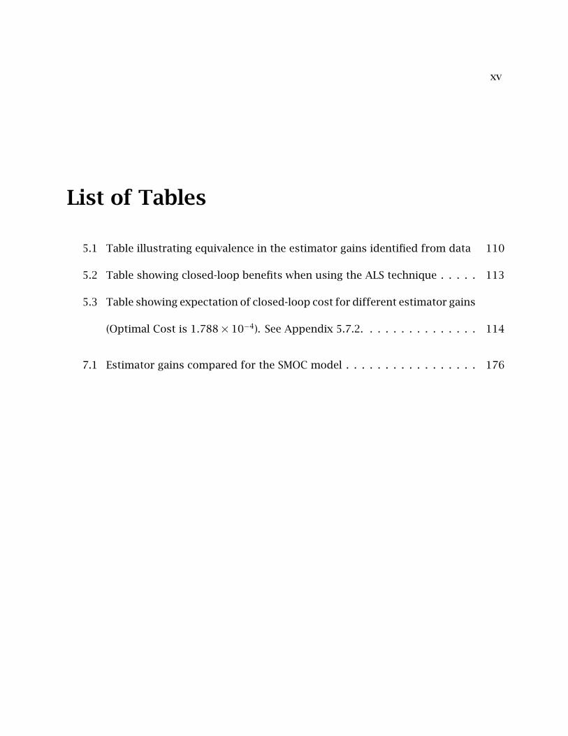
5.1 Table illustrating equivalence in the estimator gains identified from data 110

5.2 Table showing closed-loop benefits when using the ALS technique . . . . . 113

5.3 Table showing expectation of closed-loop cost for different estimator gains

(Optimal Cost is 1.788× 10−4). See Appendix 5.7.2. . . . . . . . . . . . . . . 114

7.1 Estimator gains compared for the SMOC model . . . . . . . . . . . . . . . . . 176

xvi

xvii

List of Figures

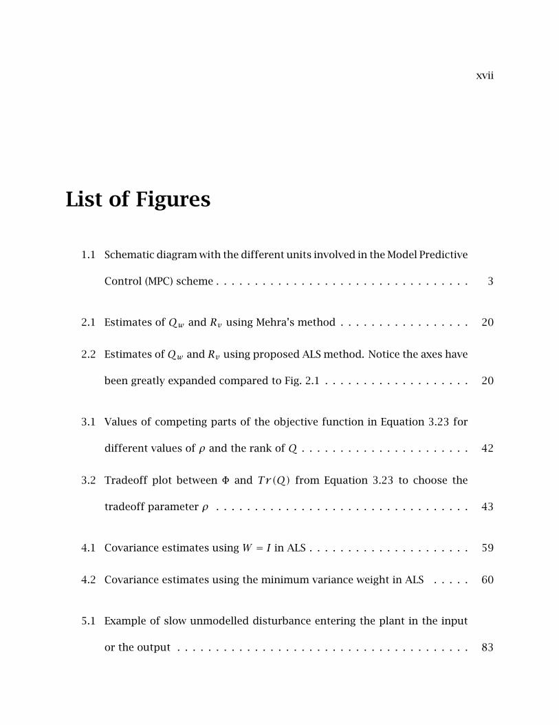
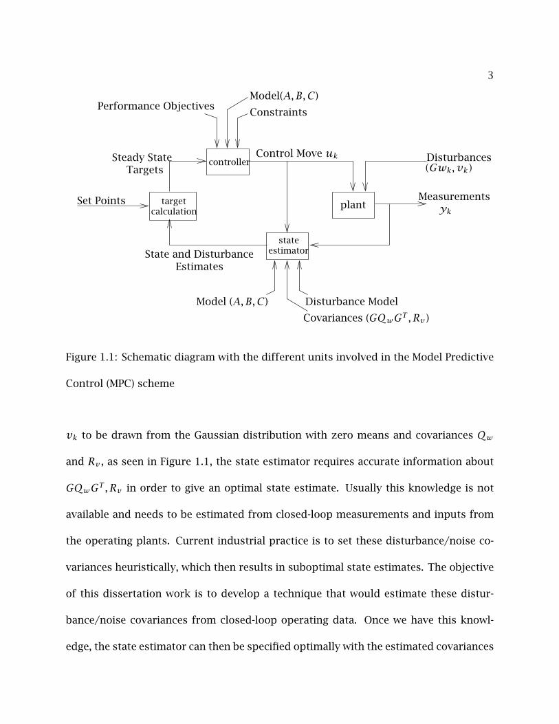
1.1 Schematic diagram with the different units involved in the Model Predictive

Control (MPC) scheme . . . . . . . . . . . . . . . . . . . . . . . . . . . . . . . . . 3

2.1 Estimates of Qw and Rv using Mehra’s method . . . . . . . . . . . . . . . . . 20

2.2 Estimates ofQw and Rv using proposed ALS method. Notice the axes have

been greatly expanded compared to Fig. 2.1 . . . . . . . . . . . . . . . . . . . 20

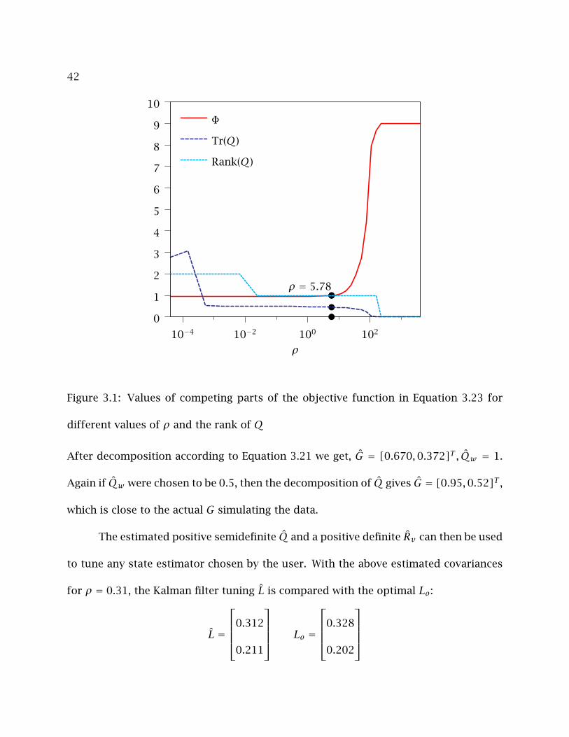
3.1 Values of competing parts of the objective function in Equation 3.23 for

different values of ρ and the rank of Q . . . . . . . . . . . . . . . . . . . . . . 42

3.2 Tradeoff plot between Φ and Tr(Q) from Equation 3.23 to choose the

tradeoff parameter ρ . . . . . . . . . . . . . . . . . . . . . . . . . . . . . . . . . 43

4.1 Covariance estimates using W = I in ALS . . . . . . . . . . . . . . . . . . . . . 59

4.2 Covariance estimates using the minimum variance weight in ALS . . . . . 60

5.1 Example of slow unmodelled disturbance entering the plant in the input

or the output . . . . . . . . . . . . . . . . . . . . . . . . . . . . . . . . . . . . . . 83

xviii

5.2 Block diagram representing parts of the Model Predictive Control (MPC)

scheme . . . . . . . . . . . . . . . . . . . . . . . . . . . . . . . . . . . . . . . . . . 85

5.3 Disturbance rejection using two disturbance models . . . . . . . . . . . . . 91

5.4 Disturbances entering the inputs . . . . . . . . . . . . . . . . . . . . . . . . . . 108

5.5 Closed-loop performance using estimator gains from the ALS technique

(D.M.=Disturbance Model) . . . . . . . . . . . . . . . . . . . . . . . . . . . . . . 112

5.6 Disturbances entering the inputs . . . . . . . . . . . . . . . . . . . . . . . . . . 113

5.7 Closed-loop performance of the estimators with gains calculated using the

ALS technique (D.M.=Disturbance Model) . . . . . . . . . . . . . . . . . . . . . 115

7.1 Strategy for calculating the time-varyingAk matrices in Equation 7.13 . . 145

7.2 Schematic diagram of the blending drum: the level and mass fractions

h,XA, XB are controlled by flows FA, FB, FD . . . . . . . . . . . . . . . . . . . . 147

7.3 Eigenvalues of (Ak −AkLkCk) plotted against time for the simulated data 150

7.4 Scatter in the covariance estimates using the ALS technique on simulated

data. The + sign shows the actual value of the covariances . . . . . . . . . . 151

7.5 Comparison of the diagonal elements of Qw and Qξ for the 5 industrial

data sets . . . . . . . . . . . . . . . . . . . . . . . . . . . . . . . . . . . . . . . . . 154

7.6 Comparison of the diagonal elements of Rv for the 5 industrial data sets 154

7.7 A snapshot of data comparing the model estimates using the initial and

the ALS covariances with the operating data in Data Set I (the y-axis is

arbitrarily scaled to disguise the original data) . . . . . . . . . . . . . . . . . 155

xix







7.10 Data Set I: Diagonal elements of the innovations autocovariance matrix at

different time lags . . . . . . . . . . . . . . . . . . . . . . . . . . . . . . . . . . . 160

7.11 Structured SMOC Model . . . . . . . . . . . . . . . . . . . . . . . . . . . . . . . 170

7.12 Disturbance entering the input in the plant . . . . . . . . . . . . . . . . . . . 174

7.13 Snapshot of the inputs . . . . . . . . . . . . . . . . . . . . . . . . . . . . . . . . 177

7.14 Snapshot of the outputs . . . . . . . . . . . . . . . . . . . . . . . . . . . . . . . 178

7.15 Data Set II: Autocovariance of the innovations at different time lags . . . . 179

7.16 Data Set III: Autocovariance of the innovations at different time lags . . . 180

7.17 Data Set IV: Autocovariance of the innovations at different time lags . . . 181

7.18 Data Set V: Autocovariance of the innovations at different time lags . . . . 182

8.1 Semi-batch CSTR with inflow of A and B . . . . . . . . . . . . . . . . . . . . . 193

8.2 MHE with a smoothing prior applied to the semi-batch reactor example . 195

8.3 PF with the optimal importance function applied to the semi-batch reactor

example . . . . . . . . . . . . . . . . . . . . . . . . . . . . . . . . . . . . . . . . . 195

xx

8.4 MHE/PF hybrid with the simplest importance function applied to the semi-

batch reactor example . . . . . . . . . . . . . . . . . . . . . . . . . . . . . . . . 196

8.5 MHE/PF hybrid with the optimal importance function applied to the semi-

batch reactor example . . . . . . . . . . . . . . . . . . . . . . . . . . . . . . . . 197

8.6 Propagation of the samples with the simplest importance function and

without resampling. Ellipses represent 95% confidence intervals for true

conditional covariances . . . . . . . . . . . . . . . . . . . . . . . . . . . . . . . . 207

8.7 Propagation of the samples with the simplest importance function and

with resampling. Ellipses represent 95% confidence intervals for the true


8.8 Propagation of the samples with the optimal importance function and with-

out resampling. Ellipses represent 95% confidence intervals for the true


8.9 Propagation of the samples with the optimal importance function and with

resampling. Ellipses represent 95% confidence intervals for the true con-

ditional covariances . . . . . . . . . . . . . . . . . . . . . . . . . . . . . . . . . . 210

1

Chapter 1

Introduction

A model of a system is one that accurately represents its dynamic behavior. With a

variety of models available, the preferred choice is often the one that provides maximum

flexibility and ease of use. Once a model is chosen, the next step is to choose a method

to estimate the parameters for the model. Parameter estimation for models is a well

researched topic, although the best model and the best estimation method are still

debated and the choice is often governed by the practicality of a method (Ljung, 1987).

The choice of the model in this dissertation work is the state-space model because of

its flexibility in representing a wide variety of special cases, which require separate

consideration in other models. For example, the ARMA models are applicable only

for stationary systems. Nonstationary systems require an additional differencing term

giving rise to ARIMA models (Box and Jenkins, 1976). State-space models are applicable

for both stationary and nonstationary systems. In addition, periodicity and time delays

are handled conveniently in state-space models by augmentation of the states. For

2

example, the linear state-space discrete-time model is given as:

xk+1 = Axk + Buk +Gwk

yk = Cxk + vk

where, the subscript ‘k’ denotes sampling of the values at times tk = k∆t with ∆t

being the sampling time. xk ∈ Rn×1 is a physical state of the system that is usually

modelled from first principles. yk ∈ Rp×1 is the vector of the measured states of the

systems. Both the states and the measurements are corrupted by additive noiseswk and

vk respectively. The inputs to the system are uk ∈ Rm×1. Such a discrete state-space

model can be easily developed from first principles ordinary differential equations and

discretized with the sampling time of ∆t.

Model Predictive Control (MPC) is one of the most widely used multivariable con-

trol technique in the chemical industry. The use of the state-space model formulation

in MPC is convenient in systems having multiple inputs and multiple outputs, as often

is the case in even the simplest of chemical units. MPC consists of three components:

the regulator, the state estimator and the target calculator. A schematic diagram of the

different units making up MPC is shown in Figure 1.1.

The state estimator unit in MPC provides feedback from past measurements and

inputs to optimally estimate the state and disturbances. Usually, the deterministic sys-

tem matrices (A, B,C) are estimated as a part of an identification scheme. The optimal-

ity of the state estimator is then based on an accurate knowledge of the actual noise

statistics entering the plant. For illustrative purposes, if we assume the noises wk and

3

(Gwk, vk)Control Move uk

yk

Performance ObjectivesModel(A,B,C)

Constraints

Disturbances

Disturbance Model

EstimatesState and Disturbance

Model (A,B,C)

Measurements

TargetsSteady State

Set Points plant

state

targetcalculation

estimator

controller

Covariances (GQwGT , Rv )

Figure 1.1: Schematic diagram with the different units involved in the Model Predictive

Control (MPC) scheme

vk to be drawn from the Gaussian distribution with zero means and covariances Qw

and Rv , as seen in Figure 1.1, the state estimator requires accurate information about

GQwGT , Rv in order to give an optimal state estimate. Usually this knowledge is not

available and needs to be estimated from closed-loop measurements and inputs from

the operating plants. Current industrial practice is to set these disturbance/noise co-

variances heuristically, which then results in suboptimal state estimates. The objective

of this dissertation work is to develop a technique that would estimate these distur-

bance/noise covariances from closed-loop operating data. Once we have this knowl-

edge, the state estimator can then be specified optimally with the estimated covariances

4

leading to better closed-loop control. Finding the number of independent disturbances

entering the plant is another issue that is addressed in this work. If the number of in-

dependent disturbances is not accurate, the result is overmodelling and nonuniqueness

in the covariance estimation. Monitoring and state estimation tools work best using

models containing the minimum number of independent disturbances.

A data-based approach to estimate the noise statistics is motivated by observing

that the parameters characterizing the noise statistics can be viewed as ‘measurable’

quantities. The effect of all noises entering the plant is reflected in the measured out-

puts from the plant. The approach taken to estimate the noise statistics from past mea-

sured outputs and inputs is to use the expected values of the autocovariances of data at

different time lags. Deviations of the model from the actual plant is accommodated in

MPC by augmenting the states in the state-space model with an integrating disturbance

model. The noise statistics for the integrated disturbance part of the state estimator is

also estimated from data using autocovariances. In this dissertation work, a technique

based on autocovariances in data is developed and applied to industrial examples. An

extension of the developed technique to nonlinear models is also developed.

For illustration, we present the simplest optimal state estimator for the linear

model. The optimal state estimator is the classical Kalman filter for unconstrained

models. The optimal state estimates are given by the following equation where the

symbol · represents an estimate:

xk+1 = Axk + Buk +ALo(yk − Cxk)

5

in which, Lo is the optimal filter gain given by solving the following equations:

Po = APoAT −APoCT (CPoCT + Rv)−1CPoAT +GQwGT

Lo = PoCT (CPoCT + Rv)−1

The estimate error covariance is Po = E[(xk − xk)(xk − xk)T ] . Thus to calculate Lo

information about the covariances Qw and Rv is needed. In the absence of this infor-

mation the covariances are set heuristically and any suboptimal filter gain L is set using

ad-hoc techniques to get reasonable performance from the closed-loop controller. The

techniques developed in this work will be used to estimate Qw and Rv from routine

operating data to use in the above Kalman filter equations.

1.1 Dissertation Overview

The subsequent chapters in this dissertation are organized as follows:

Chapter 2:

A review of the current and past literature on data-based techniques to estimate noise

statistics is presented in this chapter. The advantages of the formulation presented in

this dissertation work over other correlation based techniques in the literature is shown

through an illustrative example.

Chapter 3:

The formulation of the Autocovariance Least-Squares (ALS) technique is presented in

6

this chapter. Necessary and sufficient conditions are proved for the uniqueness of the

ALS optimization. Semidefinite constraints are added to the optimization to ensure

physical constraints on the covariances and a modification of the ALS technique is pre-

sented to estimate the number of independent disturbances from data.

Chapter 4:

This chapter is of value to an industrial practitioner interested in implementing the

ALS technique developed in Chapter 3. In this chapter issues involving practical imple-

mentation of the ALS technique is presented along with mathematical simplications to

improve the computation times. A derivation of the weighting of the ALS objective to

ensure minimum variance in the estimates is also presented along with an example.

Chapter 5:

The implementation of the ALS technique with Model Predictive Control (MPC) is de-

scribed. Integrating disturbance models in MPC ensure offset-free control in the pres-

ence of unmodelled disturbances. It is shown that the ALS technique estimates the

covariances to give optimal closed-loop controller performance even when the source

of the integrating disturbances are misassigned in the model.

Chapter 6:

The connections between maximum likelihood estimation (MLE) and the ALS technique

7

is established here. The MLE estimation for the covariances is shown to be an equivalent

ALS optimization with the least-squares objective weighted appropriately.

Chapter 7:

The main industrial applications of the ALS technique are presented. The extension of

the ALS technique to nonlinear models and an application to industrial blending drum

operating data given by ExxonMobil Chemical Company is shown. The ALS technique is

also applied to specify the estimator gains for the disturbance model structure used in

Shell’s multivariable optimization control (SMOC). Further, the connections between a

nonlinear state estimator, called the Implicit Dynamic Feedback (IDF), used at ExxonMo-

bil Chemical Company and the integrating input disturbance models in MPC is described.

Chapter 8:

Nonlinear state estimation is a challenge due to the increased complexity of the models.

A hybrid technique combining optimization based state estimation (moving horizon es-

timation) and sampling approaches to state estimation (particle filters) is described in

this chapter. The hybrid estimation has the advantage of being robust to data outliers,

bad initial guesses for the states and unmodelled disturbances in addition to being fast

and implementable in real time.

Chapter 9:

8

This chapter summarizes the main contributions in this dissertation work and outlines

recommended future work.

9

Chapter 2

Literature Review 1

Most of the literature on estimating the noise statistics from data fall under the cate-

gory of adaptive Kalman filtering. The most cited techniques in this category are based

on correlations in data. The Autocovariance Least-Squares (ALS) technique presented

in this work is also a correlation based technique. The literature on adaptive Kalman

filtering is restricted to linear systems and open-loop data. In addition, industrial appli-

cations of adaptive Kalman filtering are lacking in the literature, which we believe is due

to the omission of physical constraints such as semidefiniteness of the covariances and

thus reducing the practical impact of these techniques. We attempt in this dissertation

work to present a technique that is implementable in practical applications and also

present rigorous mathematical proofs on the applicability of the techniques.

In the rest of this chapter, we review other literature on estimating covariances

from data. In Section 2.2, we show some preliminary results to motivate the ALS tech-

nique compared to others in the literature. Since the literature is concentrated on linear

1Portions of this chapter appear in Odelson et al. (2006b)

10

systems, we refer to the following linear state-space model in the rest of this chapter:


yk = Cxk + vk

with notations defined in Chapter 1.

2.1 Review of Previous Work

A literature review of the previous works to estimate noise covariances as parameters

from data, identifies three major techniques: subspace ID, maximum likelihood estima-

tion (MLE) techniques and correlation based techniques.

2.1.1 Subspace Identification Techniques

Subspace ID is one of the most popular techniques used to estimate the system param-

eters. The popularity of the subspace ID methods stems from the fact that the calcu-

lations are based on simple projections of matrices containing readily available output

and input data. Subspace ID methods (SIMs) are however suboptimal as compared to

the traditional prediction error methods (PEMs) for model parameter estimation. The

downside of PEMs is that they require special parametrization and are nonlinear for

multivariable systems. Hence, there are no guarantees for the global optimum or for

the convergence of the optimization algorithms.

11

Starting with the state-space formulation in the innovations form:

xk+1 = Axk + Buk +ALYk

yk = Cxk +Yk(2.1)

where, L is the estimator gain and Yk = (yk − Cxk), subspace ID techniques estimate

the system matrices A,B,C, L and the covariance of the innovations given by cov(Yk) =

CPCT + Rv with P defined as the estimate error covariance.

Van Overschee and De Moor (1995) show that the subspace ID algorithms are

based on an unifying theme. Some useful subspace ID algorithms were given by Van Over-

schee and De Moor (1994); Larimore (1996, 1994); Viberg (1995) and Verhaegen (1994).

The above algorithms however give biased estimates for systems having inputs depen-

dent on the past outputs. Of recent interest Li and Qin (2001) have used principal

component analysis (PCA) for subspace ID using closed-loop data.

None of these algorithms however, estimate the noise covariances Qw and Rv .

The Kalman filter gain L is estimated directly and the estimates cov(xk+1 − Axk) and

cov(yk − Cxk) are used instead of Qw and Rv . The state estimator is also restricted

to the unconstrained Kalman filter. The covariances Qw , Rv are needed for advanced

state estimation techniques like the Moving Horizon Estimator (MHE) that can then be

used with a more general class of constrained or nonlinear systems. Estimating the

covariances in comparison to gain L, also has the advantage of monitoring the noise

entering the plant.

Another algorithm developed independent of the subspace ID techniques but

12

having an approach similar to subspace ID is the Observer/Kalman filter ID (OKID) de-

veloped by Juang et al. (1993) and Juang and Phan (1994). The difference from sub-

space ID techniques is that the OKID is applicable to closed-loop data. OKID works with

closed-loop data because the algorithm does not use projections of data matrices into

the future.

The stochastic part of the model (after subtracting the inputs) can be written as

(Juang et al., 1993):

xk+1 = (A−ALC)xk +ALyk

yk = Cxk +Yk(2.2)

Since the optimal filter gain L provides a stable estimator, we have (A−ALC)p ≈ 0 for

some p > 0. The finite output data of length Nd can then be expressed as:

yT1

yT2

. . .

yTNd

T

︸︷︷︸y

=[CAL . . . C(A−ALC)p−1AL

]︸︷︷︸

α

y0 y1 y2 . . . yNd−1

0 y0 y1 . . . yNd−2

0 0 y0...

...

0 0 0 . . . yNd−p

︸︷︷︸

Y

+

YT1

YT2

YT3

. . .

YTNd

T

︸︷︷︸ε

(2.3)

Or in more succinct form as,

y = αY + ε (2.4)

The OKID algorithm then estimates the optimal L using the following steps. For details

the reader is referred to Juang (1994) and Juang et al. (1993).

13

• Step 1: Estimate α by solving a least-squares problem starting with Equation 2.4:

α = yYT (YYT )−1

• Step 2: Re-parametrize α and form a new least-squares problem in AL

• Step 3: Solve the second least-squares problem to get an estimate of L

As opposed to the ALS technique, which solves a single least-squares optimization, the

extra steps make the OKID algorithm suboptimal.

An optimization approach to finding the Kalman filter gain L is to minimize the

mean square error of the estimate error (Astrom, 1970; Gelb, 1974).

minLE[(xk − xk)TS(xk − xk)] (2.5)

in which S is any semidefinite matrix. If S = In, then Equation 2.5 simplifies to the

Riccati equation. If S is chosen to be CCT , then 2.5 becomes a parametric optimization,

minimizing the mean squared output error i.e. minimizing E[YTkYk] or E[Tr (YkYTk )].

Using properties of the Frobenius norm, an equivalent objective is ‖ε‖2F in the limit of

large Nd (the notation ‖ · ‖F is used to denote the Frobenius norm).

Given Equation 2.4, the optimization approach in Equation 2.5 then becomes:

minL‖y−αY‖2

F (2.6)

Equation 2.6 however is a nonlinear optimization in L, as seen in Equation 2.3 and

hence, the solution of optimizing algorithms depends on the initial guess. The ALS

optimization on the other hand is convex and the convergence of the algorithms is

guaranteed for all initial guesses.

14

2.1.2 Maximum Likelihood Estimation and Grey-box Modelling

For the state-space model:


yk = Cxk + vk(2.7)

the known parameters are the matrices A,B,G,C and the unknown parameters are the

covariances Qw and Rv for the state noise wk and measurement noise vk respectively.

With a finite set of the outputs available, maximum likelihood estimation (MLE) tech-

niques aim to maximize the likelihood function. The innovations form of the likelihood

function is given as (Shumway and Stoffer, 2000):

−2lnLY (θ) =Nd∑k=1

log|Σk(θ)| +Nd∑k=1

Yk(θ)TΣk(θ)−1Yk(θ) (2.8)

in which LY (θ) is the likelihood and Σk = CPkCT + Rv . θ is the vector containing the

parameters (A, B,C,G,Qw , Rv).

If the only unknowns of interest are the covariances and the rest of the param-

eters are known with reasonable confidence, then the estimation procedure follows an

iterative scheme to minimize the objective in Equation 2.8 over the covariances Qw , Rv

with no guarantees of convergence. Note that the innovations Yk are dependent on the

parameter θ and the likelihood function is a highly nonlinear and complicated function

of θ. Newton-Raphson based algorithms (Shumway and Stoffer, 1982) and other algo-

rithms based on the expectation-maximization (EM) (Dempster et al., 1977) have been

developed in the literature to solve the above problem. All these algorithms however,

are iterative in nature and convergence is not proved.

15

A second class of problems falling under maximum likelihood estimation proce-

dures is using grey-box models. Grey-box models combine physical information with a

nonlinear state-space model yielding fewer parameters having physical meaning. Bohlin

and Graebe (1995) provide a Matlab toobox to estimate parameters in grey-box models.

The algorithm and the toolbox was further developed and improved by Kristensen et al.

(2004a,b). Their algorithm is also based on the maximization of the likelihood function.

Other than these references there has been little literature on the identification of grey-

box models. The algorithm in the Matlab toolbox involves a nonlinear optimization of

the parameters A,C,G and the noise covariances Qw , Rv in the model and a recursive

calculation of the innovations through an Extended Kalman Filter (EKF) for each guess

of the parameters. It can be easily seen that as the number of states increases the

size of the vector of unknowns θ becomes large and the estimation procedure becomes

complicated and unreliable.

For the purpose of evaluation of the MLE techniques in the literature, the deter-

ministic parts of the model i.e. A, G and C were fixed and the likelihood function was

optimized with θ = [(Qw)s , (Rv)s]. The ML estimation algorithm was tested by using a

software package called Continuous Time Stochastic Model (CTSM) developed by Kris-

tensen et al. (2004a,b) and available for download at http://www.imm.dtu.dk/ctsm/

download.html. The estimation of the covariances was highly dependent on the initial

guesses and failed to give positive semidefinite covariances for good initial guesses.

The estimated covariances were positive semidefinite only when the covariance ma-

16

trices were constrained to be diagonal. For the same set of data the Autocovariance

Least-Squares (ALS) procedure gave excellent results and the technique was executed

within short computational times.

2.1.3 Correlation Techniques

Correlation techniques are based on the idea that once the deterministic part of a plant

is modelled accurately, the residuals from the deterministic part then carry informa-

tion about the noises entering the plant. These residuals (or innovations) can then be

correlated with each other to extract information about the covariance of the distur-

bances entering the plant. The main proponent of this idea was Mehra (1970, 1971,

1972) and adapted by many others (Neethling and Young, 1974; Isaksson, 1987; Carew

and Belanger, 1973; Belanger, 1974; Noriega and Pasupathy, 1997). The ALS technique

is also a correlation based technique and initial work was presented in Odelson et al.

(2006b) and Odelson (2003). The ALS technique offers significant advantages over other

techniques in the literature. The ALS procedure solves a single least-squares problem

while the other techniques estimate the covariances in two steps. Solving a single least-

squares problem leads to smaller variance in the estimates as opposed to using two

steps. The correlation methods in the literature also, do not impose semidefinite con-

straints on the covariances leading to estimates that is not positive semidefinite for

finite sets of data.

Other literature not reviewed above are summarized below. An adaptive scheme

17

to calculate the Kalman filter gain using past innovations has been suggested by Hoang

et al. (1994, 1997). However, this method takes many samples to converge and fails to

achieve the linear minimum-variance estimate (LMVE) when deterministic disturbances

enter the plant input or output. A recent method which minimizes the output residuals

in the least-squares sense (Juang et al., 1993; Juang and Phan, 1994; Juang, 1994) was

found to be inadequate as the method does not find the covariances, but finds the filter

gain directly. An additional step of fitting a moving average model to the suboptimal

filter residuals (Chen and Huang, 1994) is not amenable for multivariable systems and

also fails given integrated white noise disturbances. Methods for estimating the state

when there are disturbances other than white noise in the plant usually involves two

steps. The disturbance model is identified first using the internal model principle and

then the disturbance is rejected using some arbitrary pole placement for the observer

that may be far from being optimal (Palaniswami and Feng, 1991; Xu and Shou, 1991).

Maryak et al. (2004) propose bounds for the Kalman filter gain for models with unknown

noise distributions. Sparks and Bernstein (1997) also use the internal model principle

to represent deterministic and sinusoidal disturbances, and their approach involves

supercompensators and dynamic compensators (Davison and Ferguson, 1981; Davison

and Goldenberg, 1975).

18

2.2 Comparison to other Correlation based Methods

In this section we present some preliminary results showing the advantages of using

the ALS technique against those in the literature. Chapter 3 provides more details on

the ALS technique formulation and the technical details.

As mentioned in Section 2.1.3, Mehra (1972); Neethling and Young (1974); Carew

and Belanger (1973) and Belanger (1974) employ a three-step procedure to estimate

(Qw , Rv ) from data. Starting with the innovations form for the state-space equation,

the steps are: (i) Solve a least-squares problem to estimate PCT from the estimated

autocovariances (P is the estimate error covariance). (ii) Use the estimated PCT to solve

for Rv using the zero lag autocovariance estimate from data. (iii) Solve a least-squares

problem to estimate Qw from the estimated PCT and Rv .

We offer two criticisms of the classic Mehra approach. The first comment con-

cerns the conditions for uniqueness of (Qw , Rv ) in Mehra’s approach. These conditions

were stated (without proof) as

1. (A,C) observable

2. A full rank

3. The number of unknown elements in the Qw matrix, g(g + 1)/2, is less than or

equal to np (n is the number of states and p is the number of outputs)

These conditions were also cited by Belanger (1974). We can easily find counterexamples

for these conditions as reported in Odelson et al. (2006b).

19

The second comment concerns the large variance associated with Mehra’s method.

This point was first made by Neethling and Young (1974), and seems to have been largely

overlooked. First, step (ii) above is inappropriate because the zero-order lag autocovari-

ance estimate, (CPCT + Rv) is not known perfectly. Second, breaking a single-stage

estimation of Qw and Rv into two stages by first finding PCT and Rv and then using

these estimates to estimate Qw in steps (i) and (iii) also increases the variance in the

estimated Qw . To quantify the size of the variance inflation associated with Mehra’s

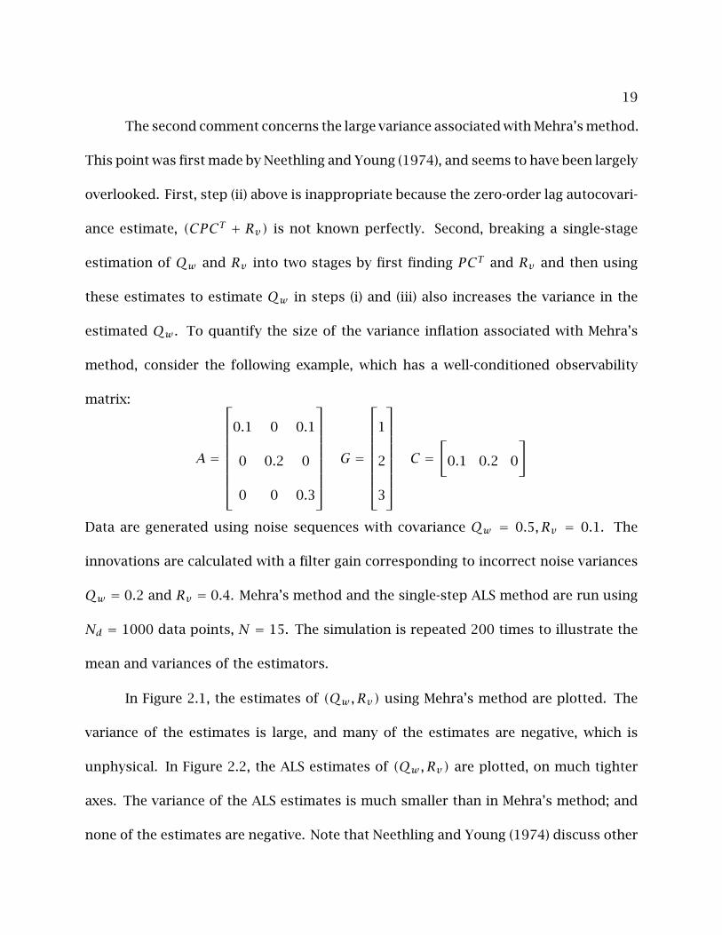
method, consider the following example, which has a well-conditioned observability

matrix:

A =

0.1 0 0.1

0 0.2 0

0 0 0.3

G =

1

2

3

C =

[0.1 0.2 0

]

Data are generated using noise sequences with covariance Qw = 0.5, Rv = 0.1. The

innovations are calculated with a filter gain corresponding to incorrect noise variances

Qw = 0.2 and Rv = 0.4. Mehra’s method and the single-step ALS method are run using

Nd = 1000 data points, N = 15. The simulation is repeated 200 times to illustrate the

mean and variances of the estimators.

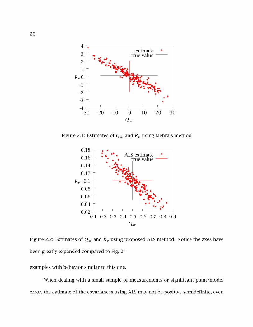
In Figure 2.1, the estimates of (Qw , Rv) using Mehra’s method are plotted. The

variance of the estimates is large, and many of the estimates are negative, which is

unphysical. In Figure 2.2, the ALS estimates of (Qw , Rv) are plotted, on much tighter

axes. The variance of the ALS estimates is much smaller than in Mehra’s method; and

none of the estimates are negative. Note that Neethling and Young (1974) discuss other

20

-4

-3

-2

-1

0

1

2

3

4

-30 -20 -10 0 10 20 30

Qw

Rv

estimatetrue value

Figure 2.1: Estimates of Qw and Rv using Mehra’s method

0.02

0.04

0.06

0.08

0.1

0.12

0.14

0.16

0.18

0.1 0.2 0.3 0.4 0.5 0.6 0.7 0.8 0.9

Qw

Rv

ALS estimatetrue value

Figure 2.2: Estimates of Qw and Rv using proposed ALS method. Notice the axes have

been greatly expanded compared to Fig. 2.1

examples with behavior similar to this one.

When dealing with a small sample of measurements or significant plant/model

error, the estimate of the covariances using ALS may not be positive semidefinite, even

21

though the variance of the estimate may be smaller than the three-step procedure. Such

estimates are physically meaningless. Most of the literature for estimating covariances

does not address this issue. A recent ad-hoc method of imposing positive semidefi-

niteness on the estimates of Rv only given in Noriega and Pasupathy (1997). The ALS

technique presented in this work as detailed in Chapter 3 impose the semidefinite con-

straints directly. The semidefinite constraints are convex in Qw , Rv and the optimiza-

tion is in the form of a semidefinite programming (SDP) problem (Vandenberghe and

Boyd, 1996). A simple path following algorithm based on Newton steps provides a

simple and efficient method to find the global optimum. Details of other semidefinite

optimization algorithms in the literature can be found in Wolkowicz et al. (2000, chap.

10).

22

23

Chapter 3

The Autocovariance Least-Squares (ALS)

Technique with Semidefinite

Programming (SDP) 1

We start with the discrete linear time-invariant state-space model given in Chapter 1:

xk+1 = Axk + Buk +Gwk (3.1a)

yk = Cxk + vk (3.1b)

in which xk, uk and yk are the state, input and output of the system at time tk. The

dimensions of the system matrices are A ∈ Rn×n, B ∈ Rn×m, G ∈ Rn×g and C ∈ Rp×n.

The noises corrupting the state and the output (wk ∈ Rg and vk ∈ Rp) are modelled

as zero-mean Gaussian noise sequences with covariances Qw and Rv respectively. The

noises wk and vk are assumed to be statistically independent for simplicity. The case

1Portions of this chapter are to appear in Rajamani and Rawlings (September, 2007)

24

where wk and vk are dependent can be handled as shown in Akesson et al. (2007). The

optimal filtering or state estimation for the model given in Equations 3.1a, 3.1b when

there are no constraints on the input and the state is given by the classical Kalman filter

(Kalman and Bucy, 1961). If the Gaussian assumption is relaxed, the Kalman filter is

the still the optimal filter among the class of all linear filters (Goodwin and Sin, 1984;

Anderson and Moore, 1979).

The G matrix shapes the disturbance wk entering the state. Physical systems

often have only a few independent disturbances which affect the states. This implies

a tall G matrix with more rows than columns. All of the correlation based techniques

in the literature described in Chapter 2, Section 2.1.3, assume that the disturbance

structure as given by the G matrix is known. In the absence of any knowledge about G

an assumption that G = I is often made, which implies that an independent disturbance

enters each of the states. This type of independence of the disturbances is unlikely for

physical reasons. There exists no technique in the literature to estimate the structure

of the disturbances entering the state, which we do in this chapter. Throughout we

assume complete knowledge about A,B,C and treat the stochastic part of the model as

the only unknowns.

The rest of the chapter is organized as follows: In Section 3.1 we give some math-

ematical preliminaries that are required to understand the rest of the chapter. Section

3.2 gives the formulation of the Autocovariance Least-Squares (ALS) technique. The

main contributions of this chapter are then presented in Sections 3.3 and 3.4. Sim-

25

ple mathematical conditions to check for uniqueness of the covariance estimates are

proved in Section 3.3 and the results used in the remaining sections. In Section 3.4 we

estimate the noise shaping matrix G from data using Semidefinite Programming (SDP).

The G matrix contains information about the disturbance structure and the number of

independent disturbances affecting the state is equal to the number of columns in G.

3.1 Background

Assumption 3.1. We assume that the pair (A,C) is observable

We use the notation xk to denote any estimate of the state xk. If L ∈ Rn×p is any

arbitrary, stable filter gain, then the state estimates are calculated recursively as:

xk+1 = Axk + Buk +AL(yk − Cxk) (3.2)

When the system is unconstrained, the optimal state estimator is the Kalman filter. For

the Kalman filter the filter gain Lo is calculated by solving the Riccati equation (also

presented in Chapter 1):

Po = APoAT −APoCT (CPoCT + Rv)−1CPoAT +GQwGT

Lo = PoCT (CPoCT + Rv)−1

(3.3)

The optimal estimate error covariance is Po = E[(xk−xk)(xk−xk)T ] calculated as above

and requires knowledge about the covariances Qw and Rv .

Given some arbitrary (stable, perhaps suboptimal) initial estimator L, we can write

the evolution of the state estimate error εk = xk − xk by subtracting Equation 3.2 from

26

3.1a and substituting 3.1b:

εk+1 = (A−ALC)︸︷︷︸A

εk +[G −AL

]︸︷︷︸

G

wkvk

Yk = Cεk + vk

(3.4)

in which Yk are the L-innovations defined as Yk Õ yk−Cxk. Note that the L-innovations

are uncorrelated in time if the initial state estimator L is optimal (i.e. L = Lo) (Anderson

and Moore, 1979). We use the term L-innovations to distinguish them from the optimal

innovations obtained by using the optimal state estimates.

Assumption 3.2. The L-innovations data Y1, · · ·YNd used in the techniques described

in this chapter are obtained after the system has reached steady state and any initial

transience is neglected since A is stable

Given a set of steady state L-innovations data Y1, · · ·YNd, we want to form a

weighted least-squares problem in the unknown disturbance covariances, GQwGT , Rv .

One of the motivations behind using a least-squares approach is to avoid a complicated

nonlinear approach required for techniques involving maximum likelihood estimation

eg. Shumway and Stoffer (1982).

In the subspace ID literature (Gevers, 2006; Van Overschee and De Moor, 1994,

1995; Viberg, 1995; Juang and Phan, 1994; Qin et al., 2005), the identification proce-

dures estimate the model and the stochastic parameters starting with the model in the

27

innovations form, which is Equation 3.2 rewritten as:

xk+1 = Axk + Buk +ALoek (3.5a)

yk = Cxk + ek (3.5b)

Here ek are the optimal innovations (as opposed to the L-innovations) and hence uncor-

related in time. The estimation of the system matrices A, B, C is carried out along with

the optimal Kalman filter gain Lo, where the · symbol denotes an estimate.

Notice the difference between Equations 3.5a,3.5b and Equations 3.1a, 3.1b. If

the subspace ID techniques are used to identify only the stochastic parameters then

the disturbance covariances as identified as ALoSLToAT instead of GQwGT for the state

noise and S instead of Rv for the measurements, where S is the covariance of ek given

by:

S = CPoCT + Rv

where, Po is defined in Equation 3.3.

Remark 3.1. As shown above, subspace ID techniques estimate a different set of covari-

ances than G,Qw , Rv . The aims of subspace ID are different and the estimates of the

stochastic parameters are simply used to compute the optimal estimator gain. Finding

the covariance parameters affecting the system (G,Qw , Rv) on the other hand provides

more flexibility in the choice of the state estimator. For example we may wish to em-

ploy a constrained, nonlinear moving horizon estimator (Rao et al., 2001). In addition

28

estimating G,Qw , Rv gives a more informative handle to monitor the disturbances than

monitoring changes in the optimal estimator gain.

Also see Remark 3.2 for requirements about exciting inputs in subspace ID tech-

niques.

3.2 The Autocovariance Least-Squares (ALS) Technique

Following the derivation along the lines of Odelson et al. (2006b), we use Equation 3.4

to write the following expectation of covariances:

E(YkYTk ) = CPCT + Rv (3.6)

E(Yk+jYTk ) = CAjPCT − CAj−1ALRv j ≥ 1 (3.7)

which are independent of k because of our steady state assumption. Again using Equa-

tion 3.4 we note that P satisfies the Lyapunov equation:

P = APAT +[G −AL

]︸︷︷︸

G

Qw 0

0 Rv

︸︷︷︸

Qw

GT (3.8)

In Odelson et al. (2006b) the autocovariance matrix was defined as:

R(N) = E

YkYTk · · · YkYTk+N−1

.... . .

...

Yk+N−1YTk · · · YkYTk

(3.9)

29

whereN is the number of lags. To avoid redundant definition of the lagged covariances,

here we use only the first block column of the autocovariance matrix R1(N):

R1(N) = E

YkYTk

...

Yk+N−1YTk

(3.10)

The formulation of the ALS technique for the full autocovariance matrix is given in

Appendix 3.6.4.

Using Equations 3.6, 3.7 and 3.8, we can write the R1(N) as:

R1(N) = OPCT + ΓRv (3.11)

in which

O =

C

CA

...

CAN−1

Γ =

Ip

−CAL...

−CAN−2AL

(3.12)

The single column block development of the ALS technique as above is preferred over

the use of the full R(N) matrix as in Odelson et al. (2006b) due to the simpler formu-

lation when using only R1(N).

In this result and those to follow, we employ the standard definitions and prop-

erties of the Kronecker product, Kronecker sum and the direct sum (Steeb (1991); Gra-

ham (1981, chap. 2) and Van Loan (2000)). If use the ‘s’ subscript to denote the

column-wise stacking of the matrix into a vector, a useful Kronecker product result

is (AXB)s = (BT ⊗A)Xs (here ⊗ is the standard symbol for the Kronecker product).

30

We then stack Equation 3.11 and use the stacked form of Equation 3.8 to substi-

tute out P :

b = (R1(N))s = [(C ⊗O)(In2 − A⊗ A)−1](GQwGT )s

+ [(C ⊗O)(In2 − A⊗ A)−1(AL⊗AL)

+ (Ip ⊗ Γ)](Rv)s

(3.13)

Now that we have Equation 3.13, we use the ergodic property of the L-innovations to

estimate the autocovariance matrixR1(N) from the given set of data (Jenkins and Watts,

1968):

E[YkYTk+j] =1

Nd − j

Nd−j∑i=1

YiYTi+j (3.14)

If Y1,Y2, · · ·YNd are the set of L-innovations calculated from data as given by Equation

3.4, and N is the window size used for the autocovariances then we define the matrix Y

as follows:

Y Õ

Y1 Y2 · · · YNd−N+1

Y2 Y3 · · · YNd−N+2

......

......

YN YN+1... YNd

(3.15)

Y ∈ Rp×n where, n Õ Nd−N +1 and p Õ Np. Using Equation 3.14, the estimate R1(N)

is then given by:

R1(N) =1

Nd −N + 1YYT1 (3.16)

31

and b = (R1(N))s . Here, Y1 is the first row block of Y also given by:

Y1 =[Ip 0 · · · 0

]︸︷︷︸

E

Y (3.17)

Given the linear relation in Equation 3.13 and the estimate b from Equation 3.16, we

can formulate the following positive semidefinite constrained least-squares problem in

the symmetric elements of the covariances GQwGT , Rv :

Φ = minGQwG,Rv

∥∥∥∥∥∥∥∥∥ADn(GQwG

T )ss

(Rv)ss

− b∥∥∥∥∥∥∥∥∥

2

W

subject to, GQwGT , Rv ≥ 0, Rv = RTv

(3.18)

The matrix W > 0 denotes the weighting of the least-squares objective. More details on

the derivation of an optimalW are given in Chapter 4, Section 4.1. Here, we introduce the

notation of (Rv)ss to denote the column-wise stacking of only the symmetric p(p+1)/2

elements of the matrix Rv (eliminating the supra-diagonal elements). More explicitly

there exists an unique matrix Dp ∈ Rp2×p(p+1)

2 called the duplication matrix (Magnus

and Neudecker, 1999, p. 49) containing ones and zeros that gives the relation (Rv)s =

Dp(Rv)ss .

Using Equation 3.13, we can then writeA explicitly as:

A=[A1 A2]

A1 =[(C ⊗O)(In2 − A⊗ A)−1]

A2 =[(C ⊗O)(In2 − A⊗ A)−1(AL⊗AL)

+ (Ip ⊗ Γ)]Dp

(3.19)

32

where, the duplication matrix Dp is included to ensure symmetry in the covariance

estimates.

The estimation method in Equation 3.18 is referred to as the Autocovariance

Least-Squares (ALS) technique in the sequel. A recent application of the ALS technique

was presented in Zhuang et al. (2007a,b). The ALS technique can also be used to estimate

the optimal filter gain when there are integrating disturbance models in model predictive

control (Chapter 5 and Rajamani et al. (2006)). One major advantage of the semidefinite

formulation of the ALS technique in Equation 3.18 is that it can be easily solved by

available semidefinite programming solvers (Wolkowicz et al., 2000; Vandenberghe and

Boyd, 1996; Boyd et al., 1994).

Remark 3.2. A significant advantage of using the ALS technique and the modifications

presented in the rest of this chapter over other identification techniques is the use of

only steady state data in the calculations. This means that unlike other identification

techniques there is no requirement for exciting inputs to be applied to the system.

3.3 Conditions for Uniqueness

In this section, we assume that the G matrix is a known Rn×g matrix. Without loss

of generality we can also assume G to be of full column rank. If G is not full column

rank then a new matrix G can be defined with its columns independent and such that

GGT = GGT .

33

We next derive simple conditions for uniqueness for the ALS problem withQw , Rv

as unknowns and a known G. In the rest of this section we also assume that the weight-

ing for the norm in the objective function is W = I.

Φ(Qw , Rv) = minQw ,Rv

∥∥∥∥∥∥∥∥∥A(Qw)ss(Rv)ss

− b∥∥∥∥∥∥∥∥∥

2

s.t. Qw , Rv ≥ 0, Rv = RTv , Qw = QTw

(3.20)

where, A =[A1(G ⊗G)Dg A2

]

Lemma 3.1. The solution of the optimization in Equation 3.20 exists for all b. The solution

is unique if and only if A in Equation 3.20 has full column rank.

Proof. Since b is a finite value calculated from data, given the bound B = Φ(Ig, Ip)

from Equation 3.20, the inequality Q,R|Φ(Q,R) ≤ B is a bounded and closed, hence

compact, set (Haaser and Sullivan, 1991, Heine-Borel Theorem, p. 85). The set Q,R|Q ≥

0, R ≥ 0,Q = QT , R = RT is the set of symmetric positive semidefinite matrices and

hence is a closed set (Wolkowicz et al., 2000, p. 69). The intersection of a compact set

and a closed set is compact (Haaser and Sullivan, 1991, p. 80). The minimization of a

continous function (Φ) on a compact set achieves its minimum on the set (Sundaram,

1996, Weierstrass Theorem, p. 90). Therefore, the solution to Equation 3.20 exists for

any set of finite measurements.

To prove uniqueness, we see that A having full column rank guarantees the ob-

jective function in Equation 3.20 to be strictly convex. The positive semidefinite con-

straints in Equation 3.20 are also convex (Vandenberghe and Boyd, 1996; Boyd et al.,

34

1994). The set Q,R|Φ(Q,R) ≤ B defines a convex set, which when intersected with

the semidefiniteness requirement still defines a convex set. Uniqueness then follows

from the existence of a bounded solution for all b and the fact that a strictly convex

objective function is subject to convex constraints (Boyd and Vandenberghe, 2004, p.

137).

Assumption 3.3. We assume that the state transition matrix A in non-singular. If the

original A is singular, then a similarity transformation can be used to eliminate the states

with zero eigenvalues and the noise covariances redefined.

Lemma 3.2. If (A,C) is observable and A is non-singular, then the matrix A in Equation

3.20 has a null space if and only if the matrixM defined by,M = (C⊗In)(In2−A⊗A)−1(G⊗

G)Dg also has a null space, and the null space ofA1(G⊗G)Dg which multiplies (Qw)ss

in Equation 3.20 is equal to the null space of M .

Proof of Lemma 3.2 is given in Appendix 3.6.1.

Theorem 3.1. If (A,C) is observable and A is non-singular, the optimization in Equation

3.20 has a unique solution if and only if dim[Null(M)] = 0, where:

M =(C ⊗ In)(In2 − A⊗ A)−1(G ⊗G)Dg

Proof. The proof follows from Lemmas 3.1 and 3.2.

Corollary 3.1. If C is full column rank (i.e. the number of sensors equal the number of

states), then the optimization in Equation 3.20 is unique.

35

Proof. C having full column rank implies M in Theorem 3.1 has full rank and hence

an empty null space. The optimization in Equation 3.20 then gives a unique solution

according to Theorem 3.1.

3.4 The ALS-SDP method

In this section the G matrix is also assumed to be unknown in addition to the Qw , Rv

matrices. An estimation technique is presented that estimates the structure of the G

matrix modelling the minimum number of independent disturbances affecting the state.

Generally a linear model of a system has many states and only a few independent

disturbances corrupting these states. Any noise wk that enters the state xk+1 is first

scaled by the G matrix and then by the C matrix before it is measured in the output

yk+1 (Equations 3.1a and 3.1b). It is unlikely to have information about the G matrix

in most applications. Information contained in the measurements is also usually not

enough to estimate a full GQwGT matrix uniquely (this can be checked using Theorem

3.1). If there are fewer sensors than the states, there can be multiple covariances that

generate the state noises making up the same output data (Corollary 3.1).

WhenG is unknown, our aim is to find the minimum rankQ (where,Q = GQwGT ).

A minimum rank Q can be decomposed as follows:

Q = GGT , Qw = I (3.21)

It should be noted that the choice Qw = I is not a binding choice for the covariance

36

because any other choice of Qw can be easily absorbed into G by redefining G1 = GQ−0.5w

so that Q = GGT = G1QwGT1 .

Having Q with minimum rank would ensure that G has the minimum number of

columns. The number of columns in the matrixG is equal to the number of independent

disturbances entering the state and equal to the rank of Q. Hence, by estimating G, we

get information about the minimum number of independent disturbances entering the

data in addition to the disturbance structure.

Remark 3.3. With reference to Equation 3.21, one might think that a more natural pro-

cedure would be to solve the ALS optimization in Equation 3.18 directly with G as the

optimization variable and constraining Qw instead of solving with Q and then following

with the decomposition. The reason for solving with Q as the optimization variable is

to avoid the nonlinearity that would be introduced if the elements of G are used as op-

timization variables and the extra flexibility in allowing for minimization of the rank of

Q.

In the development of the remaining results in this section , we take the weight

W = I. The rank can be explicitly added to the objective in Equation 3.18 through a

tradeoff parameter ρ multiplying the rank:

Φ∗ =minQ,Rv

∥∥∥∥∥∥∥∥∥A (Q)s(Rv)s

− b∥∥∥∥∥∥∥∥∥

2

︸︷︷︸Φ

+ρRank (Q)

Q,Rv ≥ 0, Q = QT , Rv = RTv

(3.22)

37

The constraints are in the form of convex Linear Matrix Inequalities (LMI) (Boyd et al.,

1994; VanAntwerp and Braatz, 2000). The norm part of the objective is also convex. The

rank however can take only integer values making the problem NP hard. The solution

of minimizing the rank subject to LMI constraints is an open research question and

current techniques are largely based on heuristics (Vandenberghe and Boyd, 1996).

Since the rank is equal to the number of nonzero eigenvalues of a matrix, a good

heuristic substitute for the rank is the sum of its eigenvalues or the trace of the matrix.

The trace of a matrix is also the largest convex envelope over the rank of the matrix

(Fazel, 2002).

Rank (Q)min ≥1

λmax(Q)Tr (Q)

The trace of a matrix is a convex function of Q. The optimization in Equation 3.22 can

be rewritten with the trace replacing the rank:

Φ1 =minQ,Rv

∥∥∥∥∥∥∥∥∥A (Q)s(Rv)s

− b∥∥∥∥∥∥∥∥∥

2

︸︷︷︸Φ

+ρTr (Q)

Q,Rv ≥ 0, Q = QT , Rv = RTv

(3.23)

Lemma 3.3. Given an optimization problem in the matrix variable X ∈ Rn×n with the

following form:

minX(AXs − b)T (AXs − b)+ ρTr (X)

subject to X ≥ 0, X = XT

38

with the matrices A and b appropriately dimensioned, the optimization can be rewritten

in the following standard primal Semidefinite Programming problem:

minx

cTx

subject to F(x) ≥ 0

where F(x) Õ F0 +m∑i=1

xiFi

with the symmetric matrices F0, · · · , Fm ∈ Rn×n and the vector c ∈ Rm chosen appro-

priately.


Given the above Lemma 3.3, if we define X = diag(Q,Rv) then Equation 3.23 is in

the form of a Semidefinite Programming (SDP) problem with A defined accordingly. We

refer to this problem as the ALS-SDP (Autocovariance Least-Squares with Semidefinite

Programming) in the sequel.

Lemma 3.4. If p < n (i.e. number of measurements is fewer than the number of states),

then the following holds for Equation 3.23:

dim[Null(A)] ≥ (n− p)(n− p + 1)/2

Proof. The dimension condition follows by substituting G = I in Lemma 3.2, noting that

(In2 − A⊗ A) is full rank and using the rank condition in Hua (1990).

Theorem 3.2. A solution (Q, Rv) to the ALS-SDP in Equation 3.23 is unique if dim[Null(M)] =

39

0 where,

M =(C ⊗ In)(In2 − A⊗ A)−1(G ⊗G)Dg

and G is any full column rank decomposition of Q = GGT (G is an unique decomposition

within an orthogonal matrix multiplication).

Proof. The function:

Φ =

∥∥∥∥∥∥∥∥∥A(G ⊗G)(Qw)s

(Rv)s

− b∥∥∥∥∥∥∥∥∥

2

is the first part of the objective in Equation 3.23 and also the same as the objective in

Equation 3.20. Following Theorem 3.1 and Lemma 3.1, dim[Null(M)] = 0 then implies

that Φ is strictly convex at the solution Qw = Ig, Rv = Rv .

The other part of the objective in Equation 3.23 i.e. Tr (Q) is linear in the variable

Q and hence is also convex. The overall objective in Equation 3.23 is then strictly convex

at the solution Q, Rv when dim[Null(M)] = 0. Uniqueness of the solution thus follows

from minimization of a strictly convex objective subject to convex constraints (Boyd

and Vandenberghe, 2004).

The ALS-SDP method gives a feasible solution for each value of the tradeoff pa-

rameter ρ by using simple Newton-like algorithms. The choice of ρ is made from a

tradeoff plot of Tr (Q) versus Φ from Equation 3.23. A good value of ρ is such that

Tr (Q) is small and any further decrease in value of Tr (Q) causes significant increase

in the value of Φ. This ensures that the rank of Q is minimized without significant

compromise on the original objective Φ (Rajamani and Rawlings, 2006).

40

The matrix inequalities Qw ≥ 0, Rv ≥ 0 can be handled by an optimization algo-

rithm adding a logarithmic barrier function to the objective. The optimization algorithm

then minimizes:

Φ1 = minQw ,Rv

Φ + ρTr (Q)− µ log

∣∣∣∣∣∣∣∣∣Q 0

0 Rv

∣∣∣∣∣∣∣∣∣ (3.24)

in which, µ is the barrier parameter and | · | denotes the determinant of the matrix

(Nocedal and Wright, 1999, chap. 17). The log-determinant barrier is an attractive

choice because it has analytical first and second derivatives. Appendix 3.6.3 lists some

useful matrix derivatives arising in the optimization in Equation 3.24. As with other

barrier techniques, with µ → 0, the solution to the SDP tends to the optimum solution.

The following approach was used to solve the barrier augmented SDP.

1. Choose a value for the tradeoff parameter ρ

2. Iteration k=0

3. Choose a starting value of µ (say µ = 100)

4. Solve the SDP and let the solution be Qk, Rk

5. Decrease value of µ (say choose the new value as µ/2)

6. Increase value of k by 1 and repeat step 4 till µ < 10−7

7. Check conditions in Theorem 3.2 for uniqueness. If the solution is not unique

then repeat with higher value for ρ.

41

Other path following type of algorithms can be found in Wolkowicz et al. (2000,

chap. 10). The convexity of Equation 3.24 ensures a unique termination of the mini-

mization algorithm. The algorithm scales efficiently for large dimensional problems.

3.4.1 Example

Let the plant be simulated using the following state-space matrices.

A =

0.733 −0.086

0.172 0.991

C =[

1 2

]G =

1

0.5

with noises drawn from the distributions:

wk ∼ N(0,0.5), vk ∼ N(0,1)

Although the data is generated by a single column G matrix, we assume G is

unknown and estimate it using the ALS-SDP procedure.

The results from the new ALS-SDP are shown in Figures 3.1 and 3.2. The plots

show that choice of ρ = 0.31 is where the Tr (Q) is the minimum with no significant

change in Φ. Also, the rank(Q) at ρ = 0.31 is 1, which is the number of independent

disturbances entering the state in the simulated data (columns of G).

Also the estimated disturbance structure and covariances using ρ = 0.31 is:

Q =

0.449 0.249

0.249 0.138

, Rv = 0.99

42

0

1

2

3

4

5

6

7

8

9

10

10−4 10−2 100 102

ρ

ρ = 5.78

Φ

Tr(Q)

Rank(Q)

Figure 3.1: Values of competing parts of the objective function in Equation 3.23 for

different values of ρ and the rank of Q

After decomposition according to Equation 3.21 we get, G = [0.670,0.372]T , Qw = 1.

Again if Qw were chosen to be 0.5, then the decomposition of Q gives G = [0.95,0.52]T ,

which is close to the actual G simulating the data.

The estimated positive semidefinite Q and a positive definite Rv can then be used

to tune any state estimator chosen by the user. With the above estimated covariances

for ρ = 0.31, the Kalman filter tuning L is compared with the optimal Lo:

L =

0.312

0.211

Lo =

0.328

0.202

43

0

0.5

1

1.5

2

2.5

3

3.5

0 2 4 6 8 10

Tr(Q

)

Fit to data Φ

ρ = 5.78

Figure 3.2: Tradeoff plot between Φ and Tr(Q) from Equation 3.23 to choose the trade-

off parameter ρ

3.5 Conclusions

Given a set of system matrices A,C , a known noise shaping matrix G and an initial

arbitrary stable filter gain L, uniqueness of the estimates of Qw and Rv using the ALS

technique can be checked using the simple conditions in Theorem 3.1. The computa-

tional burden in checking these conditions is minimal even for large dimension systems.

One of the major uncertainties in the process industries is the disturbance structure af-

fecting the significant variables of the plant. For linear models we showed that the

disturbance structure is captured accurately by the matrix G in Equation 3.1a, which

44

shapes the noises entering the states. Estimation of the minimum number of distur-

bances affecting the states is equivalent to minimizing the rank of G. An estimation

procedure using SDP and a rank heuristic was shown to give a tradeoff between fit to

the data and the minimization of the rank. The ‘knee’ of the tradeoff curve was shown

to give good estimates for the minimum number of disturbances and the disturbance

structure.

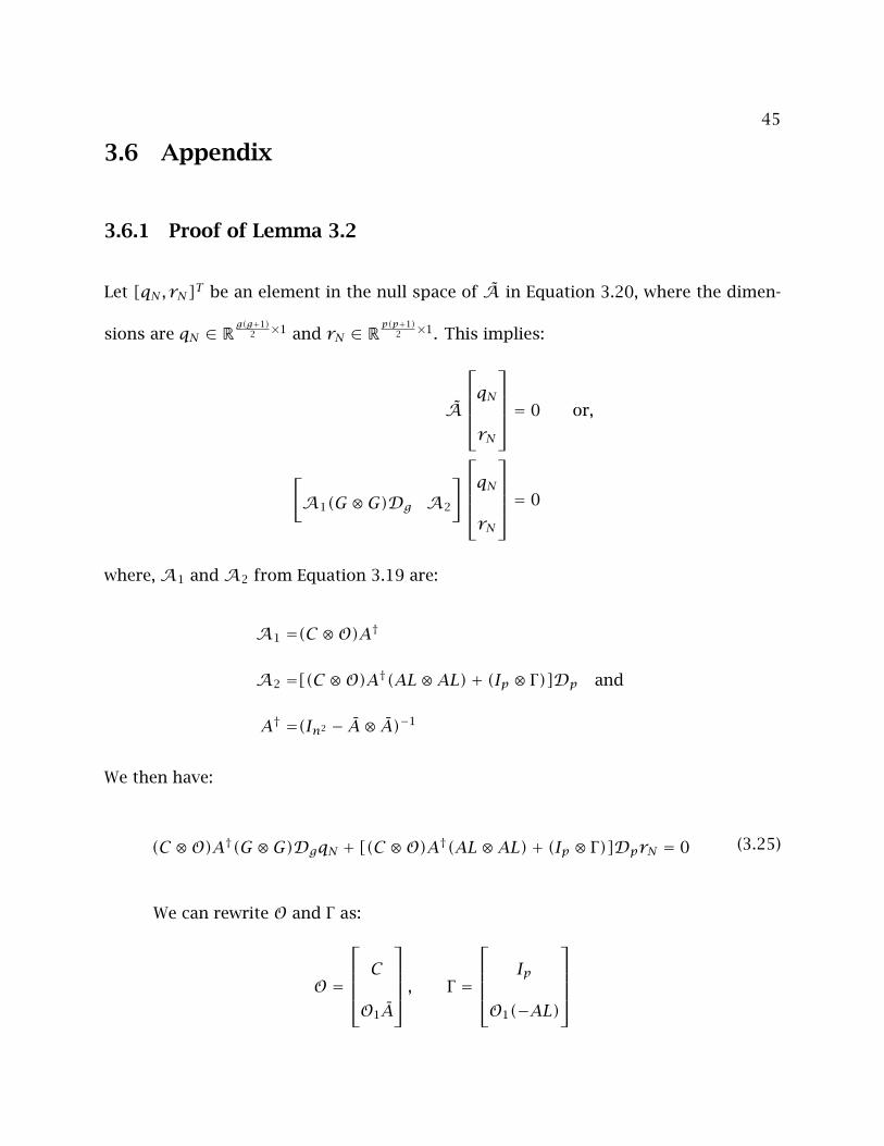
45

3.6 Appendix

3.6.1 Proof of Lemma 3.2

Let [qN , rN]T be an element in the null space of A in Equation 3.20, where the dimen-

sions are qN ∈ Rg(g+1)

2 ×1 and rN ∈ Rp(p+1)

2 ×1. This implies:

A

qNrN

= 0 or,

[A1(G ⊗G)Dg A2

]qNrN

= 0

where,A1 andA2 from Equation 3.19 are:

A1 =(C ⊗O)A†

A2 =[(C ⊗O)A†(AL⊗AL)+ (Ip ⊗ Γ)]Dp and

A† =(In2 − A⊗ A)−1

We then have:

(C ⊗O)A†(G ⊗G)DgqN + [(C ⊗O)A†(AL⊗AL)+ (Ip ⊗ Γ)]DprN = 0 (3.25)

We can rewrite O and Γ as:

O =

C

O1A

, Γ =

Ip

O1(−AL)

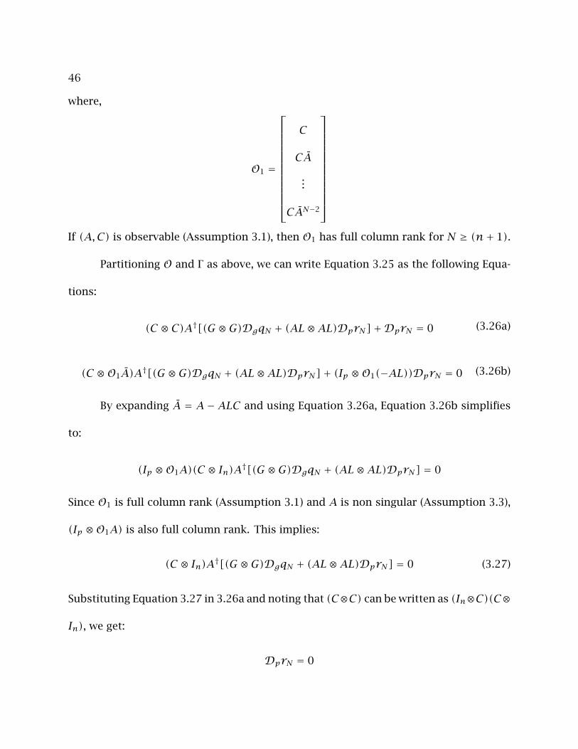
46

where,

O1 =

C

CA

...

CAN−2

If (A,C) is observable (Assumption 3.1), then O1 has full column rank for N ≥ (n+ 1).

Partitioning O and Γ as above, we can write Equation 3.25 as the following Equa-

tions:

(C ⊗ C)A†[(G ⊗G)DgqN + (AL⊗AL)DprN]+DprN = 0 (3.26a)

(C ⊗O1A)A†[(G ⊗G)DgqN + (AL⊗AL)DprN]+ (Ip ⊗O1(−AL))DprN = 0 (3.26b)

By expanding A = A − ALC and using Equation 3.26a, Equation 3.26b simplifies

to:

(Ip ⊗O1A)(C ⊗ In)A†[(G ⊗G)DgqN + (AL⊗AL)DprN] = 0

Since O1 is full column rank (Assumption 3.1) and A is non singular (Assumption 3.3),

(Ip ⊗O1A) is also full column rank. This implies:

(C ⊗ In)A†[(G ⊗G)DgqN + (AL⊗AL)DprN] = 0 (3.27)

Substituting Equation 3.27 in 3.26a and noting that (C⊗C) can be written as (In⊗C)(C⊗

In), we get:

DprN = 0

47

Equation 3.27 then simplifies to:

(C ⊗ In)A†(G ⊗G)DgqN = 0

Thus, qN is an element in the null space of M = (C ⊗ In)(In2 − A⊗ A)−1(G ⊗G)Dg and

rN = 0.

Proving the second part of the lemma is straightforward by starting with Equation

3.27 and multiplying with (In ⊗O), which is full column rank.


Since the X matrix is constrained to be symmetric, we only need to consider the sym-

metric p = n(n+1)2 elements of X. Let these symmetric elements of X be stacked in the

vector z ∈ Rp.

The original optimization in Lemma 3.3 can then be written as:

minz

(Az − b)T (Az − b)+ dTz

subject toi=p∑i=1

ziBi ≥ 0

where, A is the A modified to operate only on the symmetric elements of X, Bi ∈

Rn×n, i = 1, · · · , p are the basis matrices for a symmetric ∈ Rn×n matrix and d is

chosen appropriately such that ρTr (X) = dTz.

Using the standard technique for converting quadratic objective functions into

Linear Matrix Inequalities (see for example Vandenberghe and Boyd (1996, p. 54)), we

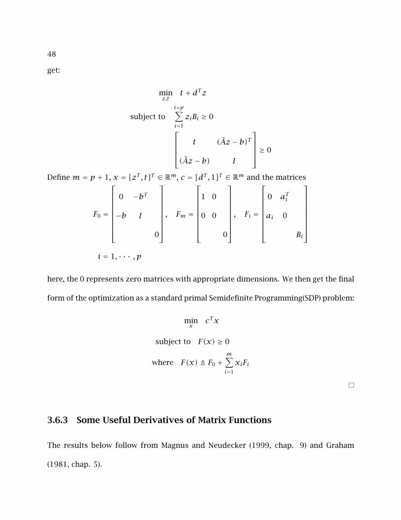
48

get:

minz,t

t + dTz

subject toi=p∑i=1

ziBi ≥ 0

t (Az − b)T

(Az − b) I

≥ 0

Define m = p + 1, x = [zT , t]T ∈ Rm, c = [dT ,1]T ∈ Rm and the matrices

F0 =

0 −bT

−b I

0

, Fm =

1 0

0 0

0

, Fi =

0 aTi

ai 0

Bi

i = 1, · · · , p

here, the 0 represents zero matrices with appropriate dimensions. We then get the final

form of the optimization as a standard primal Semidefinite Programming(SDP) problem:

minx

cTx

subject to F(x) ≥ 0

where F(x) Õ F0 +m∑i=1

xiFi

3.6.3 Some Useful Derivatives of Matrix Functions

The results below follow from Magnus and Neudecker (1999, chap. 9) and Graham

(1981, chap. 5).

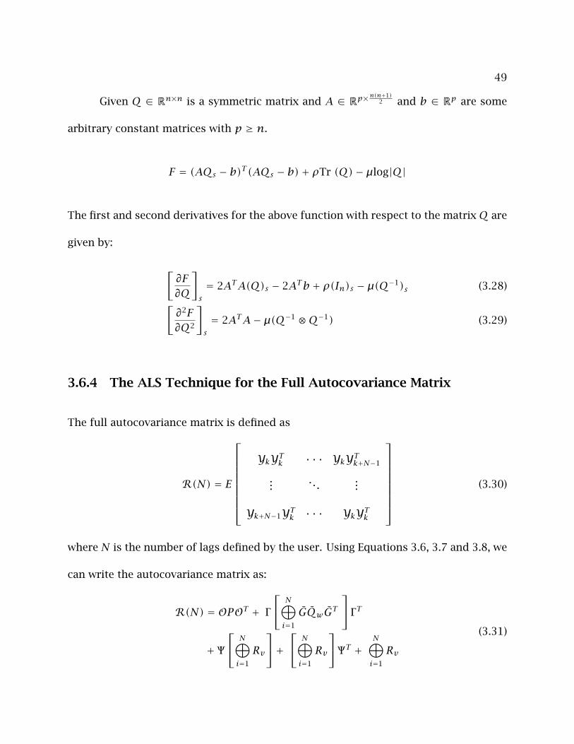
49

Given Q ∈ Rn×n is a symmetric matrix and A ∈ Rp×n(n+1)2 and b ∈ Rp are some

arbitrary constant matrices with p ≥ n.

F = (AQs − b)T (AQs − b)+ ρTr (Q)− µlog|Q|

The first and second derivatives for the above function with respect to the matrixQ are

given by:

[∂F∂Q

]s= 2ATA(Q)s − 2ATb + ρ(In)s − µ(Q−1)s (3.28)[

∂2F∂Q2

]s= 2ATA− µ(Q−1 ⊗Q−1) (3.29)

3.6.4 The ALS Technique for the Full Autocovariance Matrix

The full autocovariance matrix is defined as

R(N) = E


.... . .

...


(3.30)

where N is the number of lags defined by the user. Using Equations 3.6, 3.7 and 3.8, we

can write the autocovariance matrix as:

R(N) = OPOT + Γ

N⊕i=1

GQwGT Γ T

+ Ψ N⊕i=1

Rv

+ N⊕i=1

Rv

ΨT + N⊕i=1

Rv

(3.31)

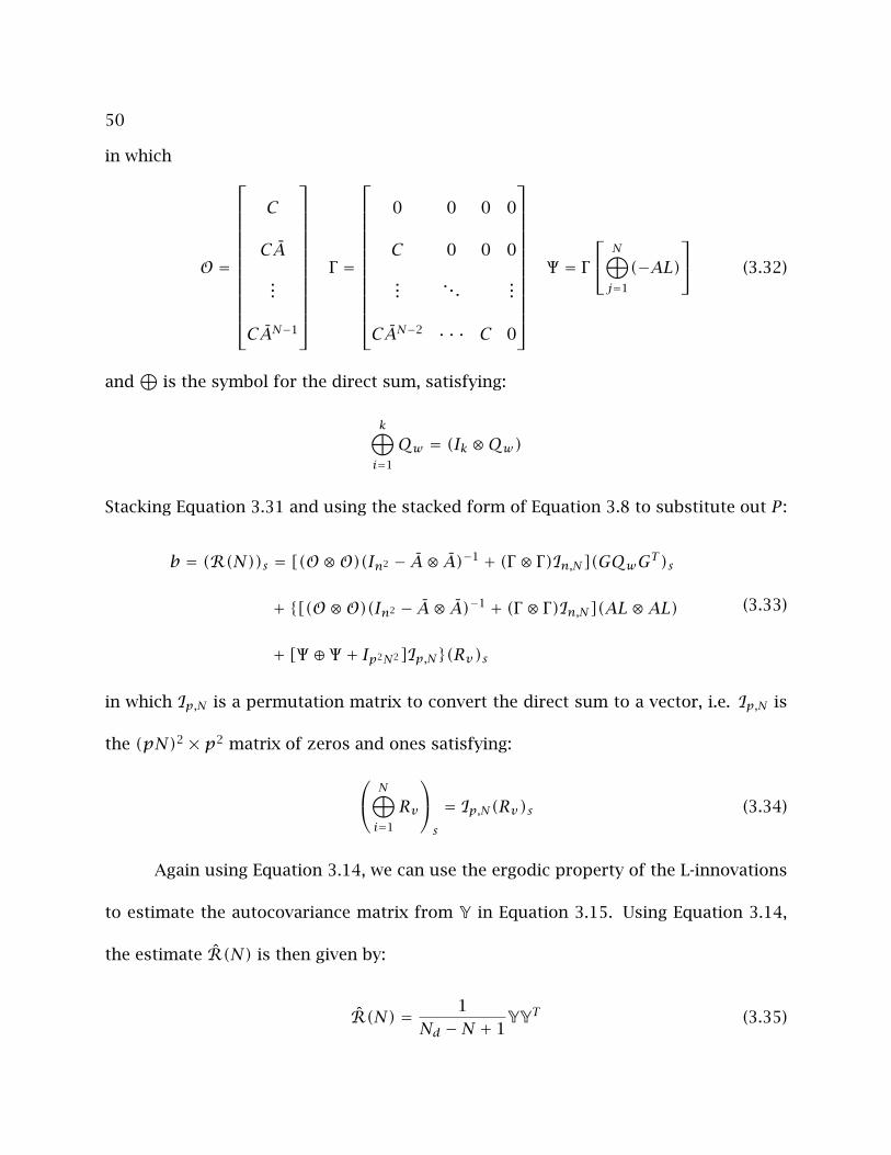
50

in which

O =

C

CA

...

CAN−1

Γ =

0 0 0 0

C 0 0 0

.... . .

...

CAN−2 · · · C 0

Ψ = Γ

N⊕j=1

(−AL) (3.32)

and⊕

is the symbol for the direct sum, satisfying:

k⊕i=1

Qw = (Ik ⊗Qw)

Stacking Equation 3.31 and using the stacked form of Equation 3.8 to substitute out P :

b = (R(N))s = [(O⊗O)(In2 − A⊗ A)−1 + (Γ ⊗ Γ)In,N](GQwGT )s

+ [(O⊗O)(In2 − A⊗ A)−1 + (Γ ⊗ Γ)In,N](AL⊗AL)

+ [Ψ ⊕ Ψ + Ip2N2]Ip,N(Rv)s

(3.33)

in which Ip,N is a permutation matrix to convert the direct sum to a vector, i.e. Ip,N is

the (pN)2 × p2 matrix of zeros and ones satisfying:

N⊕i=1

Rv

s

= Ip,N(Rv)s (3.34)

Again using Equation 3.14, we can use the ergodic property of the L-innovations

to estimate the autocovariance matrix from Y in Equation 3.15. Using Equation 3.14,

the estimate R(N) is then given by:

R(N) = 1Nd −N + 1

YYT (3.35)

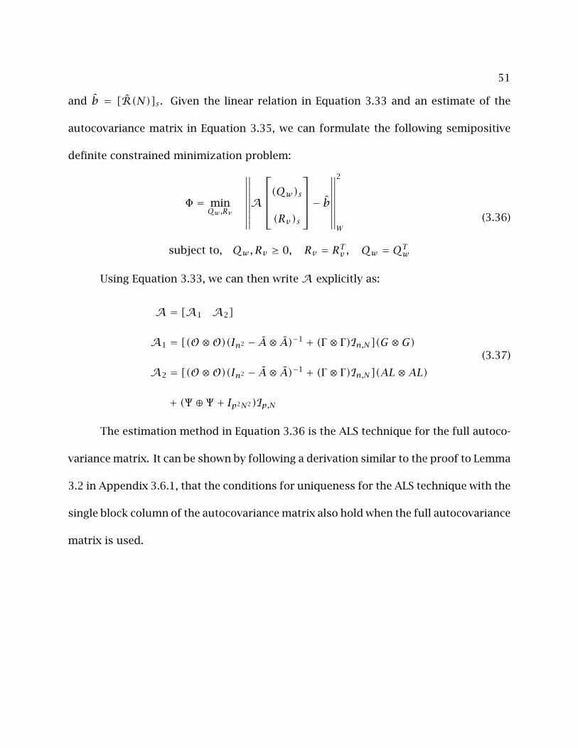
51

and b = [R(N)]s . Given the linear relation in Equation 3.33 and an estimate of the

autocovariance matrix in Equation 3.35, we can formulate the following semipositive

definite constrained minimization problem:

Φ = minQw ,Rv

∥∥∥∥∥∥∥∥∥A(Qw)s(Rv)s

− b∥∥∥∥∥∥∥∥∥

2

W

subject to, Qw , Rv ≥ 0, Rv = RTv , Qw = QTw

(3.36)

Using Equation 3.33, we can then writeA explicitly as:

A= [A1 A2]

A1 = [(O⊗O)(In2 − A⊗ A)−1 + (Γ ⊗ Γ)In,N](G ⊗G)

A2 = [(O⊗O)(In2 − A⊗ A)−1 + (Γ ⊗ Γ)In,N](AL⊗AL)

+ (Ψ ⊕ Ψ + Ip2N2)Ip,N

(3.37)

The estimation method in Equation 3.36 is the ALS technique for the full autoco-

variance matrix. It can be shown by following a derivation similar to the proof to Lemma

3.2 in Appendix 3.6.1, that the conditions for uniqueness for the ALS technique with the

single block column of the autocovariance matrix also hold when the full autocovariance

matrix is used.

52

53

Chapter 4

Optimal Weighting of the ALS Objective

and Implementation Issues 1

This chapter lists some of the implementation issues for the ALS technique described in

Chapter 3. In Section 4.1, we derive the optimal weighting matrix to calculate the linear

unbiased minimum variance estimates of the covariances. The issue ofwk and vk being

correlated with each other is covered in Section 4.2. Finally numerical simplications to

speed up the ALS algorithm are presented in Section 4.3.

1Portions of this chapter are to appear in Rajamani and Rawlings (September, 2007)

54

4.1 Minimum Variance and Optimal Weighting

Theorem 4.1. For a linear model of the form y = Ax+ e with E[e] = 0 and E[eeT ] = R,

the weighted least-squares estimator for x is:

minx‖Ax −y‖2

R−1

The weighted least-squares estimator given by

x = (ATR−1A)−1ATR−1y

then has the minimum variance among all linear unbiased estimators.

This statement is a classical generalized least-squares result for the linear re-

gression model first considered by Aitken (1935). A more recent proof can be found in

Magnus and Neudecker (1999, p. 259).

The weighted least-squares estimation of the covariances is given by the ALS

technique as shown by Equation 3.18 in Chapter 3 and repeated here for convenience:

Φ = minGQwG,Rv

∥∥∥∥∥∥∥∥∥ADn(GQwG

T )ss

(Rv)ss

− b∥∥∥∥∥∥∥∥∥

2

W

subject to, GQwGT , Rv ≥ 0, Rv = RTv

(4.1)

In Odelson et al. (2006b) and in Chapter 3, the weighting matrix W in the ALS

problem is taken to be the identity matrix. The minimum variance property for the

estimates then does not hold. We next derive the formula for the minimum variance

weighting matrix W .

55

Following the analogy of Theorem 4.1 for Equation 4.1, if b is an unbiased esti-

mator of b, then b = E[b]. Define S Õ E[(b−b)(b−b)T ] = cov(b) as the covariance of

b. Then W = S−1 is the weighting that gives minimum variance for the ALS problem. It

is shown in Odelson et al. (2006b) that b in Equation 4.1 and calculated using Equation

3.16 in Chapter 3 is an unbiased estimator.

Lemma 4.1. Given the L-innovations from Equation 3.4 and the definition of Y from

Equation 3.15 in Chapter 3, we have:

E[Y] = 0

E[YYT ] Õ E[YsYTs ] = Ω

with Ω as defined in Appendix 4.4.1 (Equation 4.25). The random matrix Y is distributed

normally with Y ∼ N(0,Ω).


Note that the formula for Ω as given by Equation 4.25 depends on the unknown distur-

bance covariances Qw , Rv and G.

Theorem 4.2. The minimum variance weight to use in the ALS objective in Equation 4.1

is given by W = S†, where,

S =T(In2p2 +K(np)(np))((KpnΩKnp)⊗ (KpnΩKnp))T T

(Nd −N + 1)2(4.2)

and Kij is the commutation matrix defined in Magnus and Neudecker (1979). T is defined

as:

T = (E⊗ Ip)(Ip2 ⊗ (In)s)T (Ip ⊗Kpn ⊗ In)

56

and E = [Ip,0 · · ·0]. n = Nd −N + 1 and p = Np

Proof. Y ∈ Rp×n is the matrix given in Equation 3.15 and is normally distributed with

mean 0 and covariance Ω as defined in Lemma 4.1. The fourth moment of Y is defined

as follows:

cov [YYT ] Õ cov((YYT )s)

The formula for the fourth moment of Y i.e cov(YYT ) for a normal distribution

is given by:

cov (YYT ) = T1(In2p2 +K(np)(np))((KpnΩKnp)⊗ (KpnΩKnp))T T1 (4.3)

where, T1 = (Ip2 ⊗ (In)s)T (Ip ⊗ Kpn ⊗ In). The formula follows from the results in

Ghazal and Neudecker (2000). See Ghazal and Neudecker (2000) for more details on the

derivation. The commutation matrix Kij is a ∈ Rij×ij matrix containing only 1’s and 0’s

and gives the following relationship between (A)s and (AT )s when A is a ∈ Ri×j matrix:

(A)s = Kij(AT )s and (AT )s = Kji(A)s .

We also have from Equations 3.16 and 3.17 in Chapter 3:

b = (YYTET )s

= (E⊗ Ip)(YYT )s

From Equation 4.3 we can then calculate the covariance of b:

S = cov(b)

= (E⊗ Ip)cov(YYT )(ET ⊗ Ip)(Nd −N + 1)2

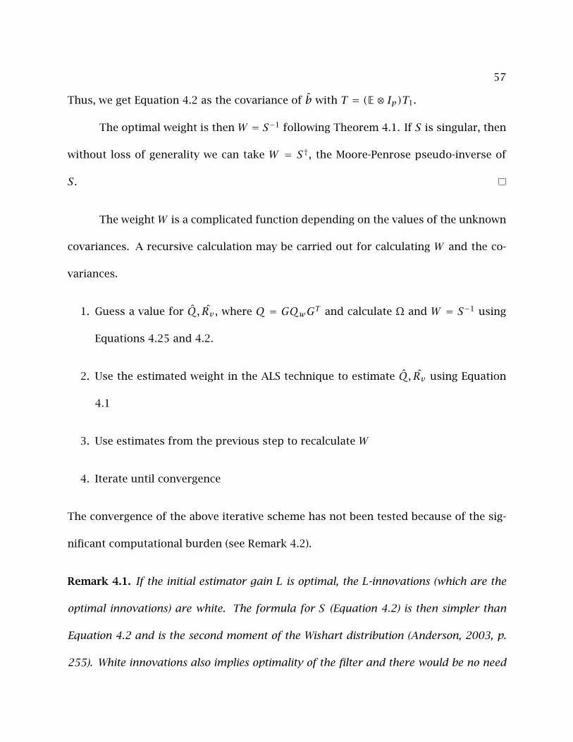
57

Thus, we get Equation 4.2 as the covariance of b with T = (E⊗ Ip)T1.

The optimal weight is then W = S−1 following Theorem 4.1. If S is singular, then

without loss of generality we can take W = S†, the Moore-Penrose pseudo-inverse of

S.

The weightW is a complicated function depending on the values of the unknown

covariances. A recursive calculation may be carried out for calculating W and the co-

variances.

1. Guess a value for Q, Rv , where Q = GQwGT and calculate Ω and W = S−1 using

Equations 4.25 and 4.2.

2. Use the estimated weight in the ALS technique to estimate Q, Rv using Equation

4.1

3. Use estimates from the previous step to recalculate W

4. Iterate until convergence

The convergence of the above iterative scheme has not been tested because of the sig-

nificant computational burden (see Remark 4.2).

Remark 4.1. If the initial estimator gain L is optimal, the L-innovations (which are the

optimal innovations) are white. The formula for S (Equation 4.2) is then simpler than

Equation 4.2 and is the second moment of the Wishart distribution (Anderson, 2003, p.

255). White innovations also implies optimality of the filter and there would be no need

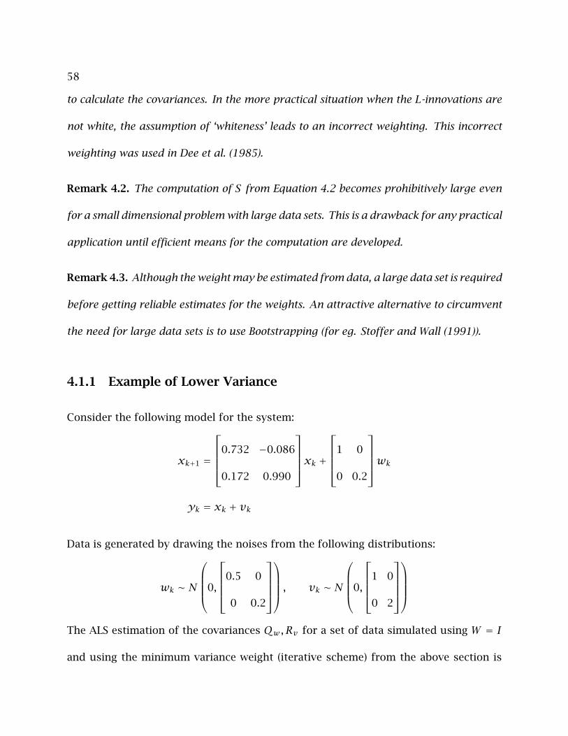
58

to calculate the covariances. In the more practical situation when the L-innovations are

not white, the assumption of ‘whiteness’ leads to an incorrect weighting. This incorrect

weighting was used in Dee et al. (1985).

Remark 4.2. The computation of S from Equation 4.2 becomes prohibitively large even

for a small dimensional problem with large data sets. This is a drawback for any practical

application until efficient means for the computation are developed.

Remark 4.3. Although the weight may be estimated from data, a large data set is required

before getting reliable estimates for the weights. An attractive alternative to circumvent

the need for large data sets is to use Bootstrapping (for eg. Stoffer and Wall (1991)).

4.1.1 Example of Lower Variance

Consider the following model for the system:

xk+1 =

0.732 −0.086

0.172 0.990

xk +1 0

0 0.2

wkyk = xk + vk

Data is generated by drawing the noises from the following distributions:

wk ∼ N

0,

0.5 0

0 0.2

, vk ∼ N

0,

1 0

0 2

The ALS estimation of the covariances Qw , Rv for a set of data simulated using W = I

and using the minimum variance weight (iterative scheme) from the above section is

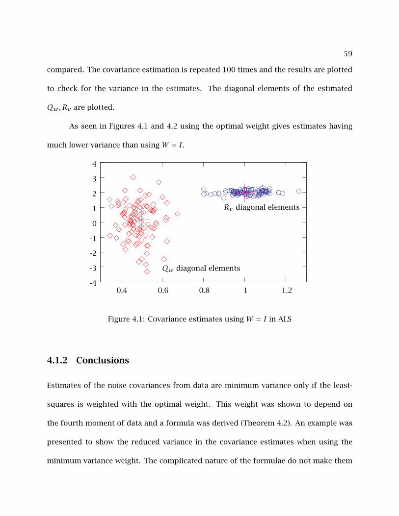
59

compared. The covariance estimation is repeated 100 times and the results are plotted

to check for the variance in the estimates. The diagonal elements of the estimated

Qw , Rv are plotted.

As seen in Figures 4.1 and 4.2 using the optimal weight gives estimates having

much lower variance than using W = I.

-4

-3

-2

-1

0

1

2

3

4

0.4 0.6 0.8 1 1.2

Qw diagonal elements

Rv diagonal elements

Figure 4.1: Covariance estimates using W = I in ALS

4.1.2 Conclusions

Estimates of the noise covariances from data are minimum variance only if the least-

squares is weighted with the optimal weight. This weight was shown to depend on

the fourth moment of data and a formula was derived (Theorem 4.2). An example was

presented to show the reduced variance in the covariance estimates when using the

minimum variance weight. The complicated nature of the formulae do not make them

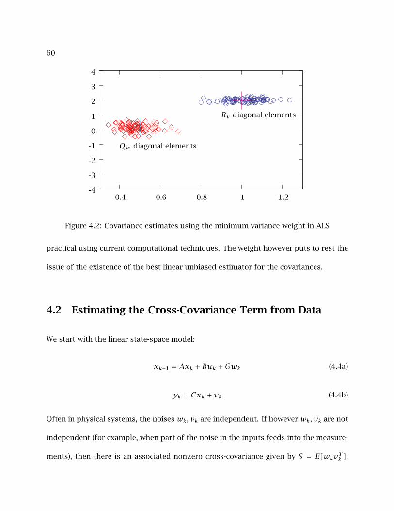
60

-4

-3

-2

-1

0

1

2

3

4

0.4 0.6 0.8 1 1.2

Qw diagonal elements

Rv diagonal elements

Figure 4.2: Covariance estimates using the minimum variance weight in ALS

practical using current computational techniques. The weight however puts to rest the

issue of the existence of the best linear unbiased estimator for the covariances.

4.2 Estimating the Cross-Covariance Term from Data

We start with the linear state-space model:

xk+1 = Axk + Buk +Gwk (4.4a)

yk = Cxk + vk (4.4b)

Often in physical systems, the noiseswk, vk are independent. If howeverwk, vk are not

independent (for example, when part of the noise in the inputs feeds into the measure-

ments), then there is an associated nonzero cross-covariance given by S = E[wkvTk ].

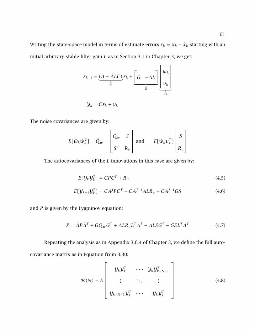
61

Writing the state-space model in terms of estimate errors εk = xk − xk starting with an

initial arbitrary stable filter gain L as in Section 3.1 in Chapter 3, we get:

εk+1 = (A−ALC)︸︷︷︸A

εk +[G −AL

]︸︷︷︸

G

wkvk

︸︷︷︸wk

Yk = Cεk + vk

The noise covariances are given by:

E[wkwTk ] = Qw =

Qw S

ST Rv

and E[wkvTk ]

SRv

The autocovariances of the L-innovations in this case are given by:

E[YkYTk ] = CPCT + Rv (4.5)

E[Yk+jYTk ] = CAjPCT − CAj−1ALRv + CAj−1GS (4.6)

and P is given by the Lyapunov equation:

P = APAT +GQwGT +ALRvLTAT −ALSGT −GSLTAT (4.7)

Repeating the analysis as in Appendix 3.6.4 of Chapter 3, we define the full auto-

covariance matrix as in Equation from 3.30:

R(N) = E


.... . .

...


(4.8)

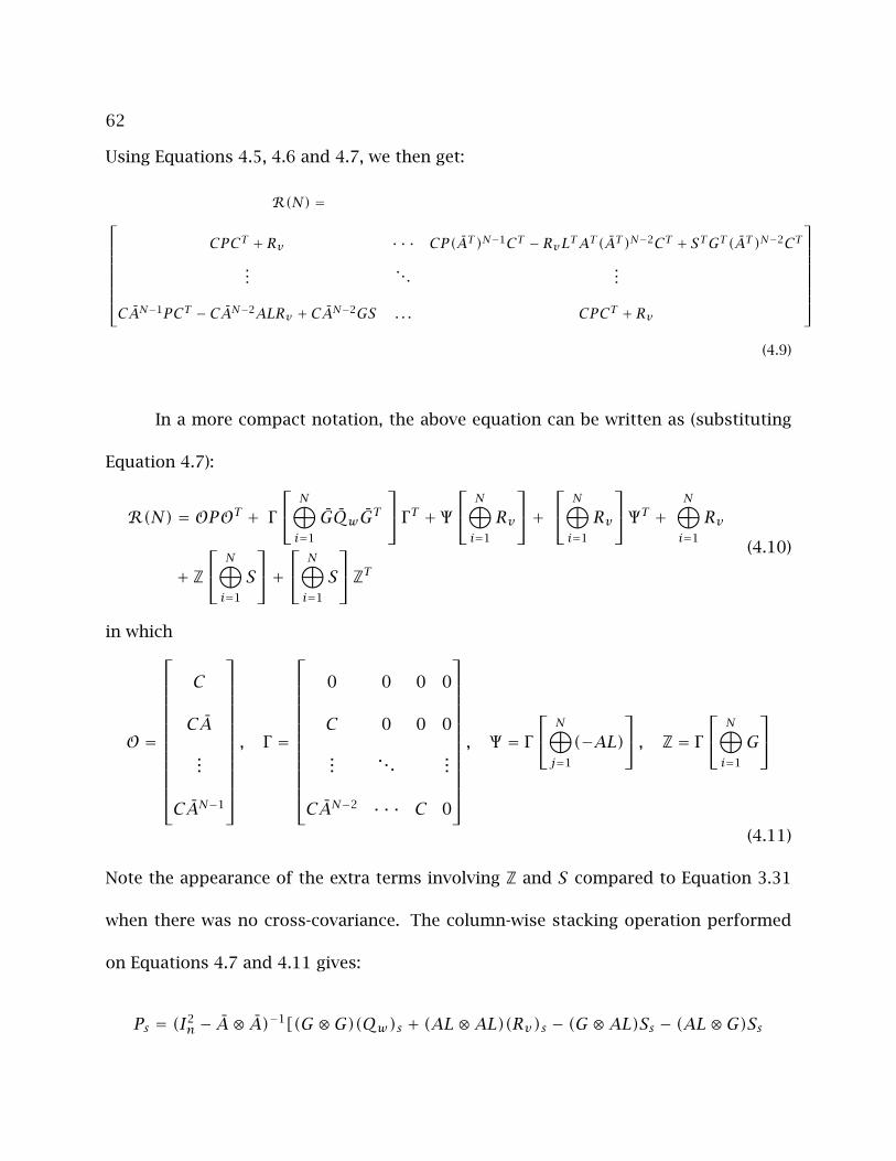
62

Using Equations 4.5, 4.6 and 4.7, we then get:

R(N) =CPCT + Rv · · · CP(AT )N−1CT − RvLTAT (AT )N−2CT + STGT (AT )N−2CT

.... . .

...

CAN−1PCT − CAN−2ALRv + CAN−2GS . . . CPCT + Rv

(4.9)

In a more compact notation, the above equation can be written as (substituting

Equation 4.7):

R(N) = OPOT + Γ

N⊕i=1

GQwGT Γ T + Ψ

N⊕i=1

Rv

+ N⊕i=1

Rv

ΨT + N⊕i=1

Rv

+ Z N⊕i=1

S

+ N⊕i=1

S

ZT(4.10)

in which

O =

C

CA

...

CAN−1

, Γ =

0 0 0 0

C 0 0 0

.... . .

...

CAN−2 · · · C 0

, Ψ = Γ

N⊕j=1

(−AL) , Z = Γ

N⊕i=1

G

(4.11)

Note the appearance of the extra terms involving Z and S compared to Equation 3.31

when there was no cross-covariance. The column-wise stacking operation performed

on Equations 4.7 and 4.11 gives:

Ps = (I2n − A⊗ A)−1[(G ⊗G)(Qw)s + (AL⊗AL)(Rv)s − (G ⊗AL)Ss − (AL⊗G)Ss

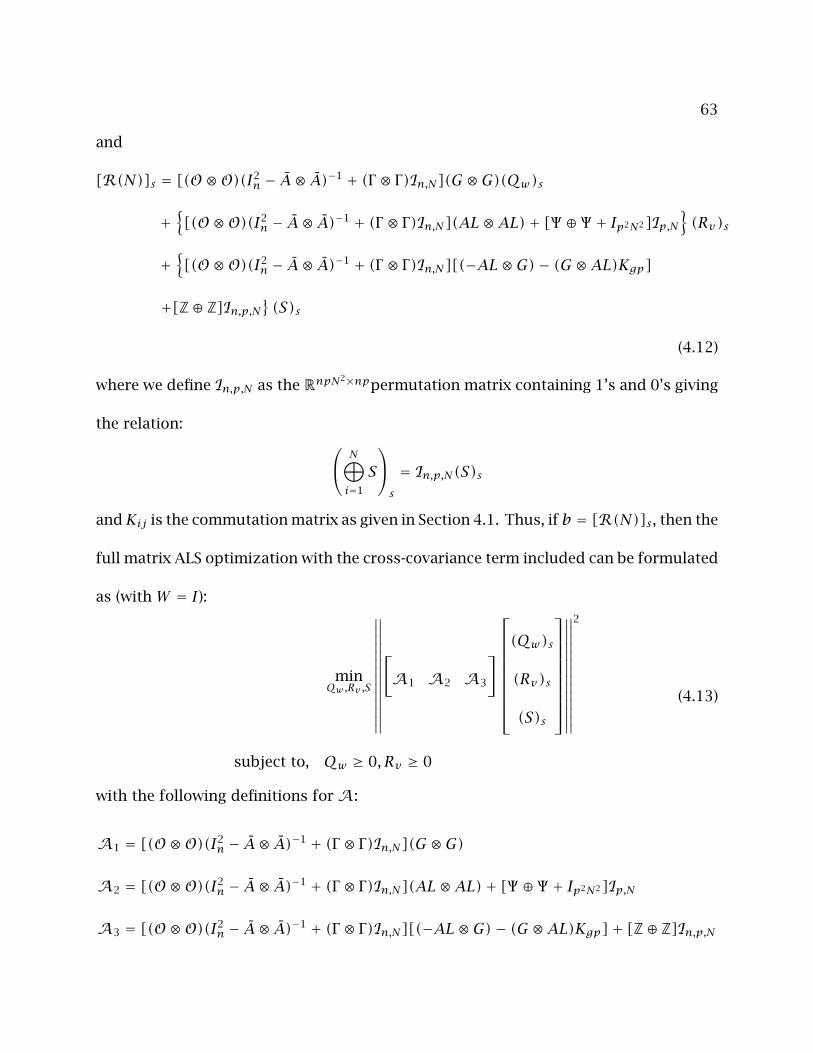
63

and

[R(N)]s = [(O⊗O)(I2n − A⊗ A)−1 + (Γ ⊗ Γ)In,N](G ⊗G)(Qw)s

+[(O⊗O)(I2

n − A⊗ A)−1 + (Γ ⊗ Γ)In,N](AL⊗AL)+ [Ψ ⊕ Ψ + Ip2N2]Ip,N(Rv)s

+[(O⊗O)(I2

n − A⊗ A)−1 + (Γ ⊗ Γ)In,N][(−AL⊗G)− (G ⊗AL)Kgp]

+[Z⊕ Z]In,p,N(S)s

(4.12)

where we define In,p,N as the RnpN2×nppermutation matrix containing 1’s and 0’s giving

the relation: N⊕i=1

S

s

= In,p,N(S)s

andKij is the commutation matrix as given in Section 4.1. Thus, if b = [R(N)]s , then the

full matrix ALS optimization with the cross-covariance term included can be formulated

as (with W = I):

minQw ,Rv ,S

∥∥∥∥∥∥∥∥∥∥∥∥∥∥

[A1 A2 A3

](Qw)s

(Rv)s

(S)s

∥∥∥∥∥∥∥∥∥∥∥∥∥∥

2

subject to, Qw ≥ 0, Rv ≥ 0

(4.13)

with the following definitions forA:

A1 = [(O⊗O)(I2n − A⊗ A)−1 + (Γ ⊗ Γ)In,N](G ⊗G)

A2 = [(O⊗O)(I2n − A⊗ A)−1 + (Γ ⊗ Γ)In,N](AL⊗AL)+ [Ψ ⊕ Ψ + Ip2N2]Ip,N

A3 = [(O⊗O)(I2n − A⊗ A)−1 + (Γ ⊗ Γ)In,N][(−AL⊗G)− (G ⊗AL)Kgp]+ [Z⊕ Z]In,p,N

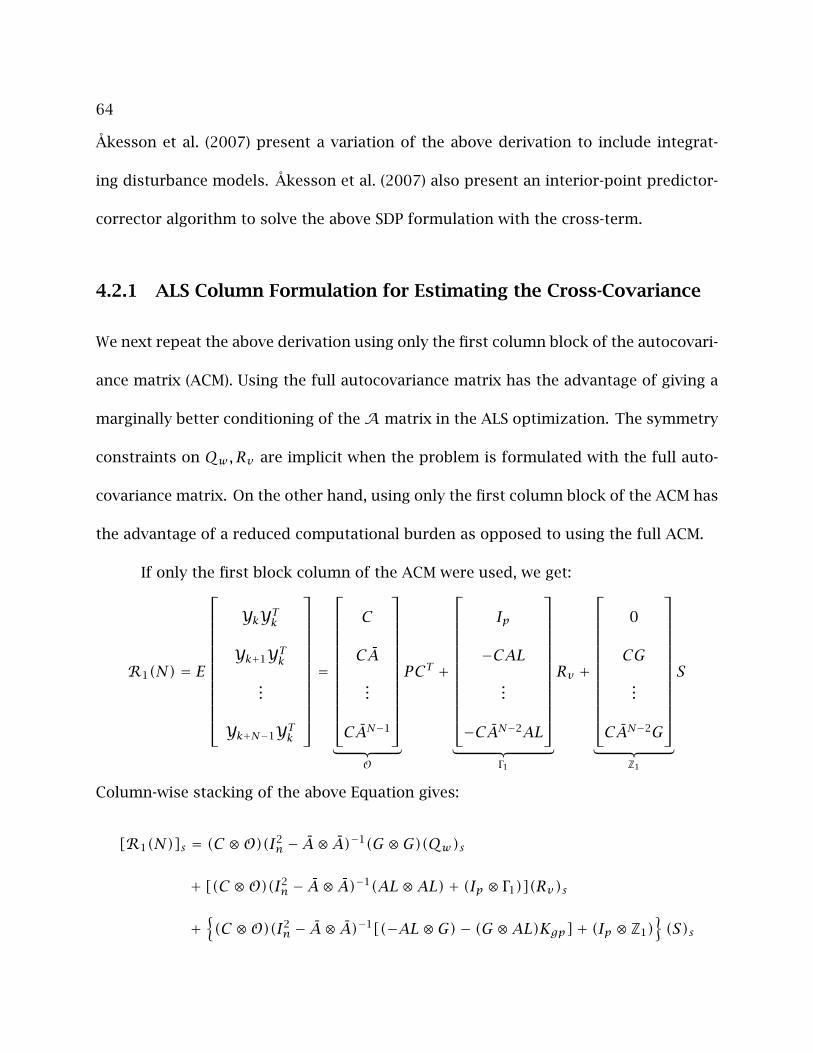
64

Akesson et al. (2007) present a variation of the above derivation to include integrat-

ing disturbance models. Akesson et al. (2007) also present an interior-point predictor-

corrector algorithm to solve the above SDP formulation with the cross-term.

4.2.1 ALS Column Formulation for Estimating the Cross-Covariance

We next repeat the above derivation using only the first column block of the autocovari-

ance matrix (ACM). Using the full autocovariance matrix has the advantage of giving a

marginally better conditioning of theAmatrix in the ALS optimization. The symmetry

constraints on Qw , Rv are implicit when the problem is formulated with the full auto-

covariance matrix. On the other hand, using only the first column block of the ACM has

the advantage of a reduced computational burden as opposed to using the full ACM.

If only the first block column of the ACM were used, we get:

R1(N) = E

YkYTk

Yk+1YTk...

Yk+N−1YTk

=

C

CA

...

CAN−1

︸︷︷︸

O

PCT +

Ip

−CAL...

−CAN−2AL

︸︷︷︸

Γ1

Rv +

0

CG

...

CAN−2G

︸︷︷︸

Z1

S

Column-wise stacking of the above Equation gives:

[R1(N)]s = (C ⊗O)(I2n − A⊗ A)−1(G ⊗G)(Qw)s

+ [(C ⊗O)(I2n − A⊗ A)−1(AL⊗AL)+ (Ip ⊗ Γ1)](Rv)s

+(C ⊗O)(I2

n − A⊗ A)−1[(−AL⊗G)− (G ⊗AL)Kgp]+ (Ip ⊗ Z1)(S)s

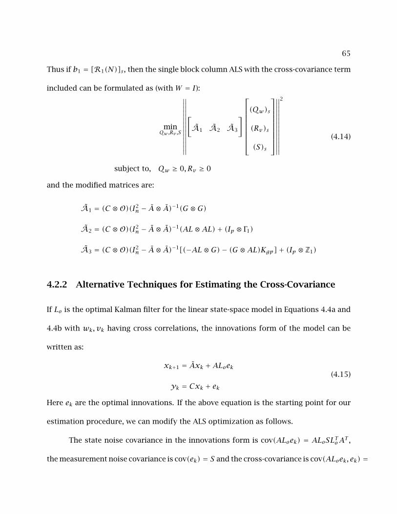
65

Thus if b1 = [R1(N)]s , then the single block column ALS with the cross-covariance term

included can be formulated as (with W = I):

minQw ,Rv ,S

∥∥∥∥∥∥∥∥∥∥∥∥∥∥

[A1 A2 A3

](Qw)s

(Rv)s

(S)s

∥∥∥∥∥∥∥∥∥∥∥∥∥∥

2

subject to, Qw ≥ 0, Rv ≥ 0

(4.14)

and the modified matrices are:

A1 = (C ⊗O)(I2n − A⊗ A)−1(G ⊗G)

A2 = (C ⊗O)(I2n − A⊗ A)−1(AL⊗AL)+ (Ip ⊗ Γ1)

A3 = (C ⊗O)(I2n − A⊗ A)−1[(−AL⊗G)− (G ⊗AL)Kgp]+ (Ip ⊗ Z1)

4.2.2 Alternative Techniques for Estimating the Cross-Covariance

If Lo is the optimal Kalman filter for the linear state-space model in Equations 4.4a and

4.4b with wk, vk having cross correlations, the innovations form of the model can be

written as:

xk+1 = Axk +ALoek

yk = Cxk + ek(4.15)

Here ek are the optimal innovations. If the above equation is the starting point for our

estimation procedure, we can modify the ALS optimization as follows.

The state noise covariance in the innovations form is cov(ALoek) = ALoSLToAT ,

the measurement noise covariance is cov(ek) = S and the cross-covariance is cov(ALoek, ek) =

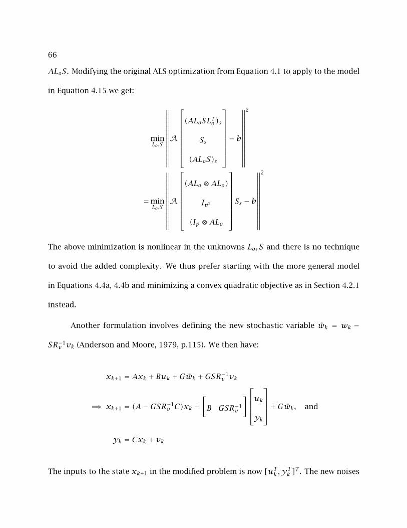
66

ALoS. Modifying the original ALS optimization from Equation 4.1 to apply to the model

in Equation 4.15 we get:

minLo,S

∥∥∥∥∥∥∥∥∥∥∥∥∥∥A

(ALoSLTo )s

Ss

(ALoS)s

− b

∥∥∥∥∥∥∥∥∥∥∥∥∥∥

2

=minLo,S

∥∥∥∥∥∥∥∥∥∥∥∥∥∥A

(ALo ⊗ALo)

Ip2

(Ip ⊗ALo

Ss − b

∥∥∥∥∥∥∥∥∥∥∥∥∥∥

2

The above minimization is nonlinear in the unknowns Lo, S and there is no technique

to avoid the added complexity. We thus prefer starting with the more general model

in Equations 4.4a, 4.4b and minimizing a convex quadratic objective as in Section 4.2.1

instead.

Another formulation involves defining the new stochastic variable wk = wk −

SR−1v vk (Anderson and Moore, 1979, p.115). We then have:

xk+1 = Axk + Buk +Gwk +GSR−1v vk

=⇒ xk+1 = (A−GSR−1v C)xk +

[B GSR−1

v

]ukyk

+Gwk, and

yk = Cxk + vk

The inputs to the state xk+1 in the modified problem is now [uTk , yTk ]T . The new noises

67

wk and vk are not cross correlated. We have:

E

wkvk

[wTk vTk

] =Qw − SR

−1v ST 0

0 Rv

However, we need prior information about the measurement noise covariance Rv to

formulate the problem in this manner. An alternative procedure would be recursive

substitution of the estimated Rv starting with an initial guess. Again the recursive

procedure makes the problem similar to a nonlinear estimation problem as opposed to

the convex ALS technique in Section 4.2.1.

4.2.3 Conditions for Uniqueness with Cross-Covariance term

The uniqueness of the ALS optimization with the cross-covariance term has no known

simple form as in the case when there are no cross correlations. The covariance esti-

mates are unique if the matrix A =[A1 A2 A3

]for the full autocovariance matrix

formulation of the ALS has full column rank. Similar conditions can be written when

using only the first block of the autocovariance matrix.

4.3 Mathematical Simplications to Speed up the Computa-

tion of the ALS Technique

We present here mathematical simplications that can be included in the ALS code to

obtain efficient and fast solutions to the optimization.

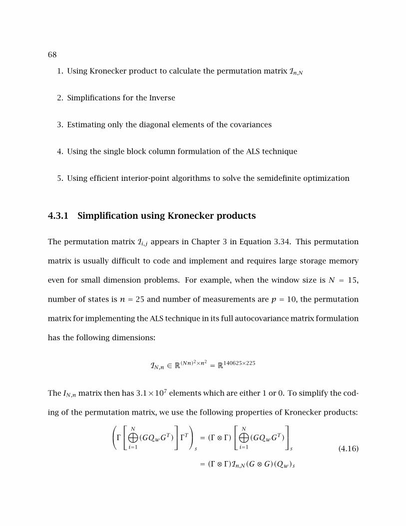
68

1. Using Kronecker product to calculate the permutation matrix In,N

2. Simplifications for the Inverse

3. Estimating only the diagonal elements of the covariances

4. Using the single block column formulation of the ALS technique

5. Using efficient interior-point algorithms to solve the semidefinite optimization

4.3.1 Simplification using Kronecker products

The permutation matrix Ii,j appears in Chapter 3 in Equation 3.34. This permutation

matrix is usually difficult to code and implement and requires large storage memory

even for small dimension problems. For example, when the window size is N = 15,

number of states is n = 25 and number of measurements are p = 10, the permutation

matrix for implementing the ALS technique in its full autocovariance matrix formulation

has the following dimensions:

IN,n ∈ R(Nn)2×n2 = R140625×225

The IN,n matrix then has 3.1×107 elements which are either 1 or 0. To simplify the cod-

ing of the permutation matrix, we use the following properties of Kronecker products:Γ N⊕i=1

(GQwGT )

Γ Ts

= (Γ ⊗ Γ) N⊕i=1

(GQwGT )

s

= (Γ ⊗ Γ)In,N(G ⊗G)(Qw)s

(4.16)

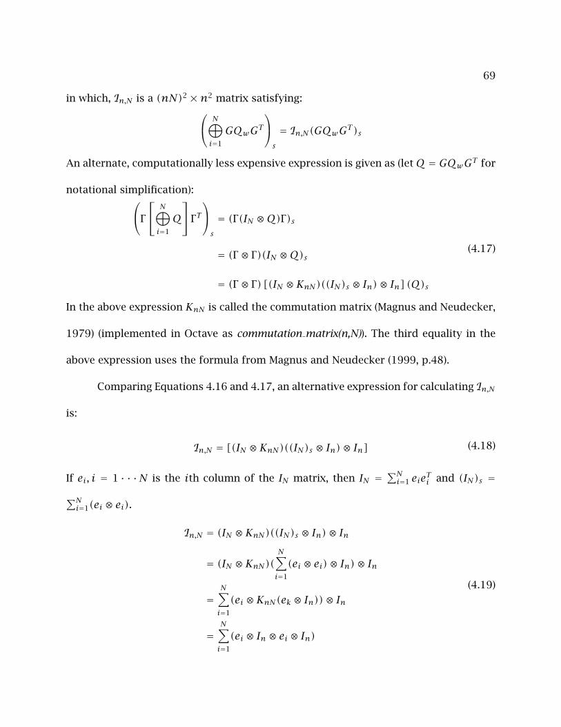
69

in which, In,N is a (nN)2 ×n2 matrix satisfying: N⊕i=1

GQwGTs

= In,N(GQwGT )s

An alternate, computationally less expensive expression is given as (letQ = GQwGT for

notational simplification):Γ N⊕i=1

Q

Γ Ts

= (Γ(IN ⊗Q)Γ)s

= (Γ ⊗ Γ)(IN ⊗Q)s

= (Γ ⊗ Γ) [(IN ⊗KnN)((IN)s ⊗ In)⊗ In] (Q)s

(4.17)

In the above expression KnN is called the commutation matrix (Magnus and Neudecker,

1979) (implemented in Octave as commutation matrix(n,N)). The third equality in the

above expression uses the formula from Magnus and Neudecker (1999, p.48).

Comparing Equations 4.16 and 4.17, an alternative expression for calculating In,N

is:

In,N = [(IN ⊗KnN)((IN)s ⊗ In)⊗ In] (4.18)

If ei, i = 1 · · ·N is the ith column of the IN matrix, then IN =∑Ni=1 eie

Ti and (IN)s =∑N

i=1(ei ⊗ ei).

In,N = (IN ⊗KnN)((IN)s ⊗ In)⊗ In

= (IN ⊗KnN)(N∑i=1

(ei ⊗ ei)⊗ In)⊗ In

=N∑i=1

(ei ⊗KnN(ek ⊗ In))⊗ In

=N∑i=1

(ei ⊗ In ⊗ ei ⊗ In)

(4.19)

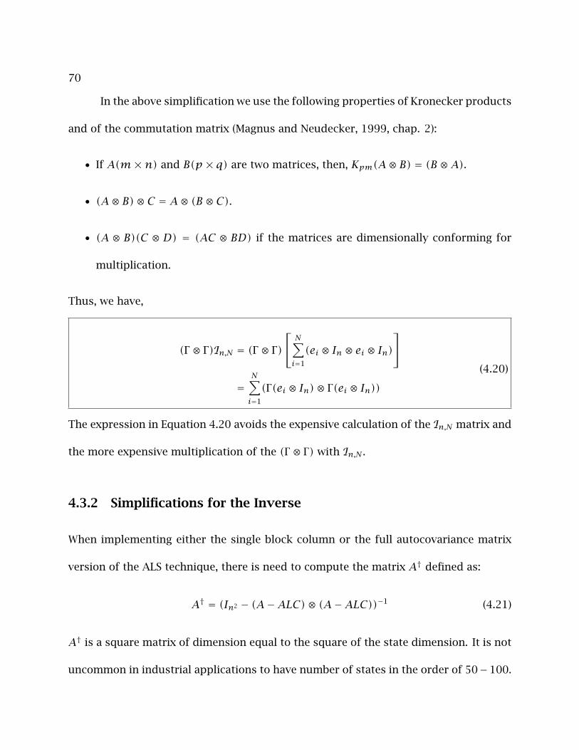
70

In the above simplification we use the following properties of Kronecker products

and of the commutation matrix (Magnus and Neudecker, 1999, chap. 2):

• If A(m×n) and B(p × q) are two matrices, then, Kpm(A⊗ B) = (B ⊗A).

• (A⊗ B)⊗ C = A⊗ (B ⊗ C).

• (A ⊗ B)(C ⊗ D) = (AC ⊗ BD) if the matrices are dimensionally conforming for

multiplication.

Thus, we have,

(Γ ⊗ Γ)In,N = (Γ ⊗ Γ) N∑i=1

(ei ⊗ In ⊗ ei ⊗ In)

=N∑i=1

(Γ(ei ⊗ In)⊗ Γ(ei ⊗ In))(4.20)

The expression in Equation 4.20 avoids the expensive calculation of the In,N matrix and

the more expensive multiplication of the (Γ ⊗ Γ) with In,N .

4.3.2 Simplifications for the Inverse

When implementing either the single block column or the full autocovariance matrix

version of the ALS technique, there is need to compute the matrix A† defined as:

A† = (In2 − (A−ALC)⊗ (A−ALC))−1 (4.21)

A† is a square matrix of dimension equal to the square of the state dimension. It is not

uncommon in industrial applications to have number of states in the order of 50−100.

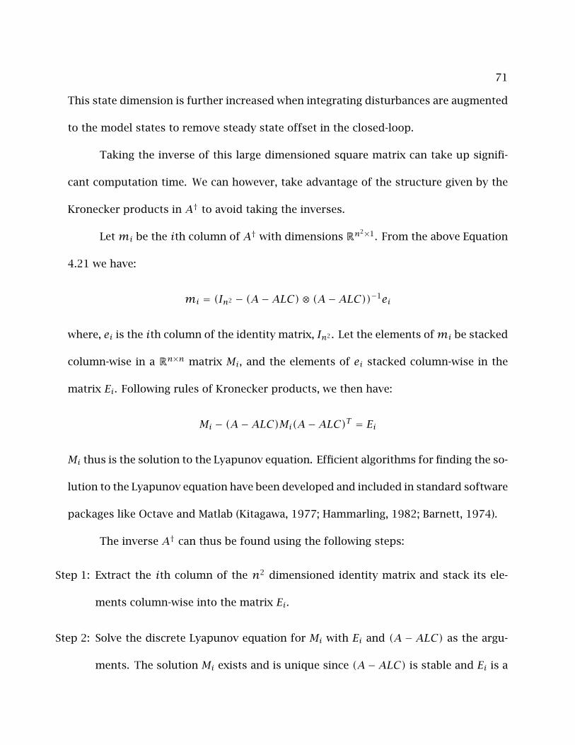
71

This state dimension is further increased when integrating disturbances are augmented

to the model states to remove steady state offset in the closed-loop.

Taking the inverse of this large dimensioned square matrix can take up signifi-

cant computation time. We can however, take advantage of the structure given by the

Kronecker products in A† to avoid taking the inverses.

Letmi be the ith column of A† with dimensions Rn2×1. From the above Equation

4.21 we have:

mi = (In2 − (A−ALC)⊗ (A−ALC))−1ei

where, ei is the ith column of the identity matrix, In2 . Let the elements ofmi be stacked

column-wise in a Rn×n matrix Mi, and the elements of ei stacked column-wise in the

matrix Ei. Following rules of Kronecker products, we then have:

Mi − (A−ALC)Mi(A−ALC)T = Ei

Mi thus is the solution to the Lyapunov equation. Efficient algorithms for finding the so-

lution to the Lyapunov equation have been developed and included in standard software

packages like Octave and Matlab (Kitagawa, 1977; Hammarling, 1982; Barnett, 1974).

The inverse A† can thus be found using the following steps:

Step 1: Extract the ith column of the n2 dimensioned identity matrix and stack its ele-

ments column-wise into the matrix Ei.

Step 2: Solve the discrete Lyapunov equation for Mi with Ei and (A − ALC) as the argu-

ments. The solution Mi exists and is unique since (A−ALC) is stable and Ei is a

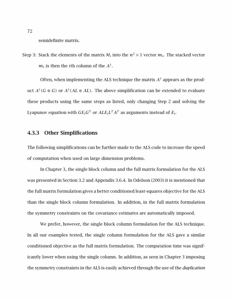
72

semidefinite matrix.

Step 3: Stack the elements of the matrix Mi into the n2× 1 vectormi. The stacked vector

mi is then the ith column of the A†.

Often, when implementing the ALS technique the matrix A† appears as the prod-

uct A†(G ⊗ G) or A†(AL ⊗ AL). The above simplification can be extended to evaluate

these products using the same steps as listed, only changing Step 2 and solving the

Lyapunov equation with GEiGT or ALEiLTAT as arguments instead of Ei.

4.3.3 Other Simplifications

The following simplifications can be further made to the ALS code to increase the speed

of computation when used on large dimension problems.

In Chapter 3, the single block column and the full matrix formulation for the ALS

was presented in Section 3.2 and Appendix 3.6.4. In Odelson (2003) it is mentioned that

the full matrix formulation gives a better conditioned least-squares objective for the ALS

than the single block column formulation. In addition, in the full matrix formulation

the symmetry constraints on the covariance estimates are automatically imposed.

We prefer, however, the single block column formulation for the ALS technique.

In all our examples tested, the single column formulation for the ALS gave a similar

conditioned objective as the full matrix formulation. The computation time was signif-

icantly lower when using the single column. In addition, as seen in Chapter 3 imposing

the symmetry constraints in the ALS is easily achieved through the use of the duplication

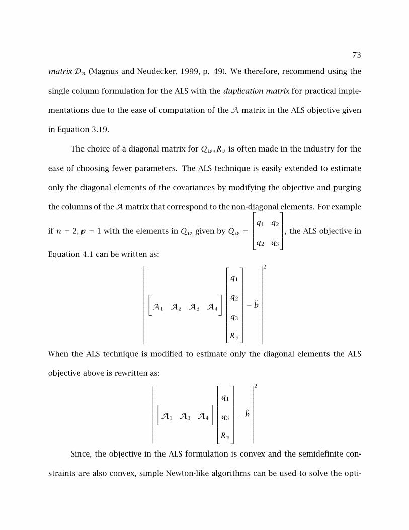
73

matrix Dn (Magnus and Neudecker, 1999, p. 49). We therefore, recommend using the

single column formulation for the ALS with the duplication matrix for practical imple-

mentations due to the ease of computation of the A matrix in the ALS objective given

in Equation 3.19.

The choice of a diagonal matrix for Qw , Rv is often made in the industry for the

ease of choosing fewer parameters. The ALS technique is easily extended to estimate

only the diagonal elements of the covariances by modifying the objective and purging

the columns of theAmatrix that correspond to the non-diagonal elements. For example

if n = 2, p = 1 with the elements in Qw given by Qw =

q1 q2

q2 q3

, the ALS objective in

Equation 4.1 can be written as:∥∥∥∥∥∥∥∥∥∥∥∥∥∥∥∥∥∥∥

[A1 A2 A3 A4

]

q1

q2

q3

Rv

− b

∥∥∥∥∥∥∥∥∥∥∥∥∥∥∥∥∥∥∥

2

When the ALS technique is modified to estimate only the diagonal elements the ALS

objective above is rewritten as:∥∥∥∥∥∥∥∥∥∥∥∥∥∥

[A1 A3 A4

]q1

q3

Rv

− b

∥∥∥∥∥∥∥∥∥∥∥∥∥∥

2

Since, the objective in the ALS formulation is convex and the semidefinite con-

straints are also convex, simple Newton-like algorithms can be used to solve the opti-

74

mization. More complex algorithms that are specific to semidefinite programming can

also be applied to improve the speed and efficiency of the algorithms. Akesson et al.

(2007) present a new predictor-corrector algorithm for solving the ALS optimization

also including the cross-terms for the covariances. Many efficient algorithms for solving

semidefinite programming problems and optimization problems involving linear matrix

inequalities (LMIs) are available in the literature. The following references present some

recent progress in the field of semidefinite optimization: Boyd et al. (1994); Wolkow-

icz et al. (2000); Vandenberghe and Boyd (1995); VanAntwerp and Braatz (2000) and

Vandenberghe and Boyd (1996).

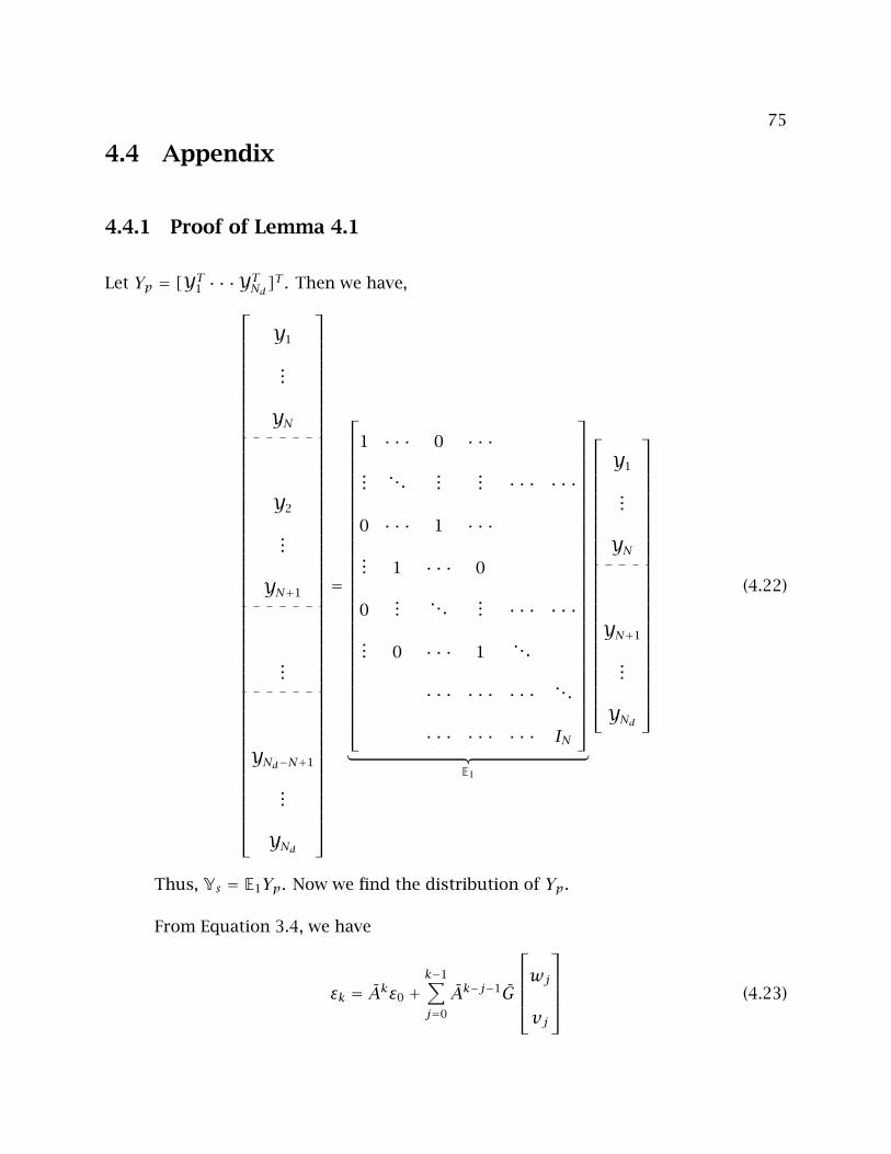
75

4.4 Appendix


Let Yp = [YT1 · · ·YTNd]T . Then we have,

Y1

...

YN

Y2

...

YN+1

...

YNd−N+1

...

YNd

=

1 · · · 0 · · ·...

. . ....

... · · · · · ·

0 · · · 1 · · ·... 1 · · · 0

0...

. . .... · · · · · ·

... 0 · · · 1. . .

· · · · · · · · · . . .

· · · · · · · · · IN

︸︷︷︸

E1

Y1

...

YN

YN+1

...

YNd

(4.22)

Thus, Ys = E1Yp. Now we find the distribution of Yp.

From Equation 3.4, we have

εk = Akε0 +k−1∑j=0

Ak−j−1G

wjvj

(4.23)

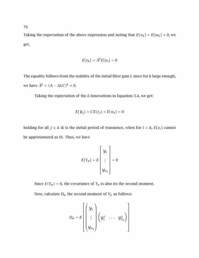
76

Taking the expectation of the above expression and noting that E[vk] = E[wk] = 0, we

get,

E[εk] = AkE[ε0] = 0

The equality follows from the stability of the initial filter gain L since for k large enough,

we have Ak = (A−ALC)k ≈ 0.

Taking the expectation of the L-innovations in Equation 3.4, we get:

E[Yj] = CE[εj]+ E[vk] = 0

holding for all j ≥ k (k is the initial period of transience, when for i < k, E[εi] cannot

be approximated as 0). Thus, we have

E[Yp] = E

Y1

...

YNd

= 0

Since E(Yp) = 0, the covariance of Yp is also its the second moment.

Now, calculate Ωp the second moment of Yp as follows:

Ωp = E

Y1

...

YNd

(YT1 · · · YTNd

)

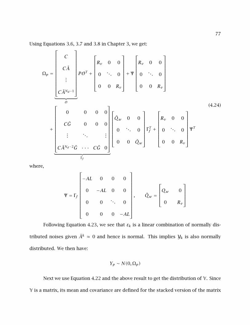
77

Using Equations 3.6, 3.7 and 3.8 in Chapter 3, we get:

Ωp =

C

CA

...

CANd−1

︸︷︷︸

O

POT +

Rv 0 0

0. . . 0

0 0 Rv

+ Ψ

Rv 0 0

0. . . 0

0 0 Rv

+

0 0 0 0

CG 0 0 0

.... . .

...

CANd−2G · · · CG 0

︸︷︷︸

Γf

Qw 0 0

0. . . 0

0 0 Qw

Γ Tf +

Rv 0 0

0. . . 0

0 0 Rv

ΨT

(4.24)

where,

Ψ = Γf

−AL 0 0 0

0 −AL 0 0

0 0. . . 0

0 0 0 −AL

, Qw =

Qw 0

0 Rv

Following Equation 4.23, we see that εk is a linear combination of normally dis-

tributed noises given Ak ≈ 0 and hence is normal. This implies Yk is also normally

distributed. We then have:

Yp ∼ N(0,Ωp)

Next we use Equation 4.22 and the above result to get the distribution of Y. Since

Y is a matrix, its mean and covariance are defined for the stacked version of the matrix

78

i.e. Ys . Given the linear relationship between Yp and Ys , we get,

Ys ∼ N(0,E1ΩpET1 )

Thus, the covariance of Y is:

Ω = E1ΩpET1 (4.25)

where Ωp is given by Equation 4.24 and E1 is defined in Equation 4.22.

79

Chapter 5

Applying the ALS Technique for

Misassigned Disturbance Models in

Offset-free Model Predictive Control 1

Model Predict ive Control (MPC) has emerged as one of the most important advanced

control methods in the chemical industry (Qin and Badgwell, 2003). MPC casts the

control problem in the form of an optimization, which makes it convenient to handle

constraints and nonlinear models explicitly. Most current formulations of MPC have a

state estimator along with the dynamic constrained regulator and a target calculator.

Nominal asymptotic stability for a deterministic linear MPC was shown by Rawlings

and Muske (1993) under the assumption that the model is known perfectly and there

is full state information. With random disturbances however, the state is no longer

1Portions of this chapter are to appear in Rajamani et al. (August, 2007)

80

known exactly and one requires dynamic feedback from the measurements to update

the current estimate of the state. The function of the state estimator is to reconcile the

past and current measurements to estimate the current state of the system. Nominal

stability of the state estimator combined with the regulator was shown by Scokaert et al.

(1997). The regulator and the target calculator require only estimates of the current

state and the disturbance to make a prediction of optimal control moves over a future

horizon.

Any correlated disturbance, that enters the plant and is not included in the model,

results in biased predicted states. It is customary to assume that the disturbance enters

through the inputs or the outputs. The bias can be removed by using the predicted and

measured outputs to estimate the disturbance. In the target calculator formulation, the

state is augmented with integrating disturbances. The target calculator then ensures

offset free control in presence of unmodelled disturbances (Muske and Rawlings, 1993a)

by shifting the steady state target for the regulator depending on the estimate of the

bias (with the assumption that the bias remains constant in the future). The integrat-

ing disturbance can be added either to the input (Davison and Smith, 1971; Morari and

Stephanopoulos, 1980), to the output (Richalet et al., 1978; Cutler and Ramaker, 1980)

or a combination of both (Marquis and Broustail, 1988; Pannocchia and Rawlings, 2002;

Muske and Badgwell, 2002). Most industrial MPC implementations add the bias term

to the output (Qin and Badgwell, 2003; Downs, 1999). Pannocchia and Rawlings (2002)

and Muske and Badgwell (2002) independently derived rank conditions that should be

81

satisfied for the disturbance models to ensure offset-free control. They also point out

the lack of consensus in the literature on the choice of the disturbance model. Their

examples show significant difference in the closed-loop behavior of the controller de-

pending on the choice of the disturbance model. Recently Pannocchia and Bemporad

(2007) present a method for a combined design of a disturbance model and its observer

by solving an appropriateH∞ control problem. Their work, however, neglects stochastic

disturbances that enter the state and the measured outputs.

The main contribution of this chapter is to show that for linear models, the choice

of the disturbance model does not affect the performance of the closed-loop when the

estimator gain is found from appropriately chosen noise covariances. The equivalence

in the estimator gains is shown by appealing to realization theory (Ho and Kalman,

1966). Subsequently the performance of any regulator that is a feedback on the current

estimate of the state remains unaffected by the choice of the disturbance model. The

covariances can be estimated from data using autocovariances at different time lags us-

ing the ALS technique developed in Chapter 3. The state estimator gain thus determined

from the estimated covariances gives optimal closed-loop performance.

The rest of the chapter is organized as follows: In Section 5.1 the equations for

estimation, regulation and target calculation in MPC are given. We motivate the rest of

the chapter by examining the consequences of an incorrect disturbance model in Section

5.2. Section 5.3 formulates the equivalence transformation between arbitrary choices

of the disturbance models. Section 5.4 presents the autocovariance least-squares (ALS)

82

technique for estimating the covariances for incorrectly chosen disturbance models

followed by examples in section 5.5. Finally, conclusions are presented in Section 5.6.

5.1 Background

We start with the following discrete-time state-space description of the model as given

in Chapter 1:

Plant:


yk = Cxk + vk(5.1)

with the usual notations and dimensions. Let the covariances of wk, vk be Qw , Rv re-

spectively and also assume that wk, vk are not cross correlated as in Chapter 3. The

pair (A,C) is assumed to be observable and the pair (A, B) assumed controllable. Let

yck be the set of controlled outputs that are a subset of the measurements yk given by

yck = Hyk. In the rest of this chapter we assume without loss of generality that the set

of controlled outputs are the same as the measured outputs with H = I. We also use

the term “measurements” and “outputs” interchangeably to mean yk. The analysis in

this chapter remains the same when yck is only a subset of yk.

As before, we assume that the deterministic parameters (A, B,C) of the plant in

Equation 5.1 are known or estimated using identification procedures and the stochastic

parameters G,Qw , Rv are unknown. Even though the deterministic parameters may be

known perfectly, unmodelled disturbances can enter through the inputs or the outputs

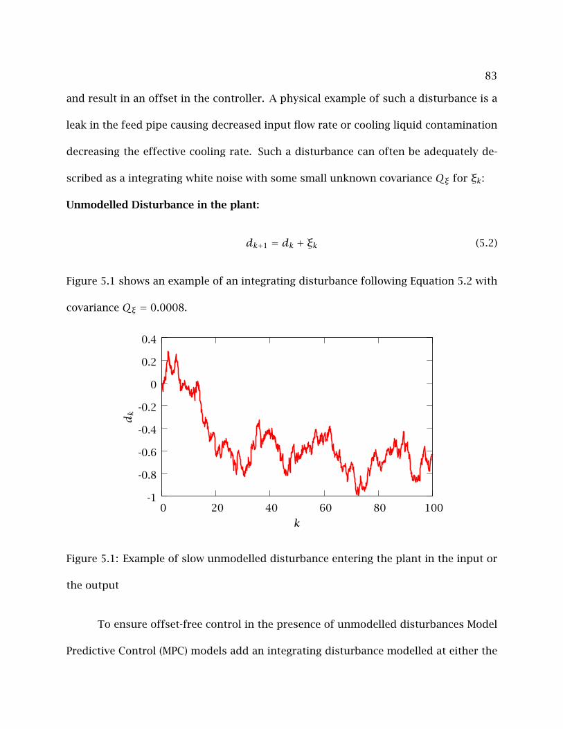
83

and result in an offset in the controller. A physical example of such a disturbance is a

leak in the feed pipe causing decreased input flow rate or cooling liquid contamination

decreasing the effective cooling rate. Such a disturbance can often be adequately de-

scribed as a integrating white noise with some small unknown covariance Qξ for ξk:

Unmodelled Disturbance in the plant:

dk+1 = dk + ξk (5.2)

Figure 5.1 shows an example of an integrating disturbance following Equation 5.2 with

covariance Qξ = 0.0008.

-1

-0.8

-0.6

-0.4

-0.2

0

0.2

0.4

0 20 40 60 80 100

dk

k

Figure 5.1: Example of slow unmodelled disturbance entering the plant in the input or

the output

To ensure offset-free control in the presence of unmodelled disturbances Model

Predictive Control (MPC) models add an integrating disturbance modelled at either the

84

inputs or the outputs of the system (Francis and Wonham, 1975, 1976). Let dk ∈ Rnd

be the integrating disturbance entering the state through the matrix Bd ∈ Rn×nd and

the measurement through Cd ∈ Rp×nd . The state x in the model is augmented with the

integrating disturbance.

Augmented Model:xd

k+1

=

A Bd

0 I

︸︷︷︸

Aa

xd

k

+

B0

uk +G 0

0 I

︸︷︷︸

Ga

wξ

k

yk =[C Cd

]︸︷︷︸

Ca

xd

k

+ vk

(5.3)

The choice of the structure of the disturbance Bd, Cd is usually unknown and a general

unstructured disturbance model can have disturbances entering both the states and

the outputs. The conditions on the models Bd, Cd for detectability and to ensure offset

free control were proved by Pannocchia and Rawlings (2002) and Muske and Badgwell

(2002).

In addition to the covariances GQwGT , Rv , the covariance Qξ of the disturbance

ξk is also required now to specify the state estimator gain. Usual choices for the distur-

bance model are (Muske and Rawlings, 1993a):

1. Bd = 0, Cd = I called the output disturbance model, or

2. Bd = B,Cd = 0 called the input disturbance model

The number of disturbances nd has to be chosen as nd = p to ensure zero offset in all

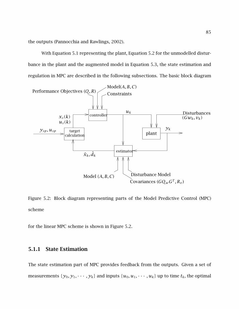
85

the outputs (Pannocchia and Rawlings, 2002).

With Equation 5.1 representing the plant, Equation 5.2 for the unmodelled distur-

bance in the plant and the augmented model in Equation 5.3, the state estimation and

regulation in MPC are described in the following subsections. The basic block diagram

xs(k)uk

us(k)yk

xk, dk

ysp, usp

(Gwk, vk)

Performance Objectives (Q,R)Model(A,B,C)

Constraints

Disturbances

calculationtarget

controller

estimator

plant

Disturbance ModelModel (A,B,C)Covariances (GQwGT , Rv )

Figure 5.2: Block diagram representing parts of the Model Predictive Control (MPC)

scheme

for the linear MPC scheme is shown in Figure 5.2.

5.1.1 State Estimation

The state estimation part of MPC provides feedback from the outputs. Given a set of

measurements y0, y1, · · · , yk and inputs u0, u1, · · · , uk up to time tk, the optimal

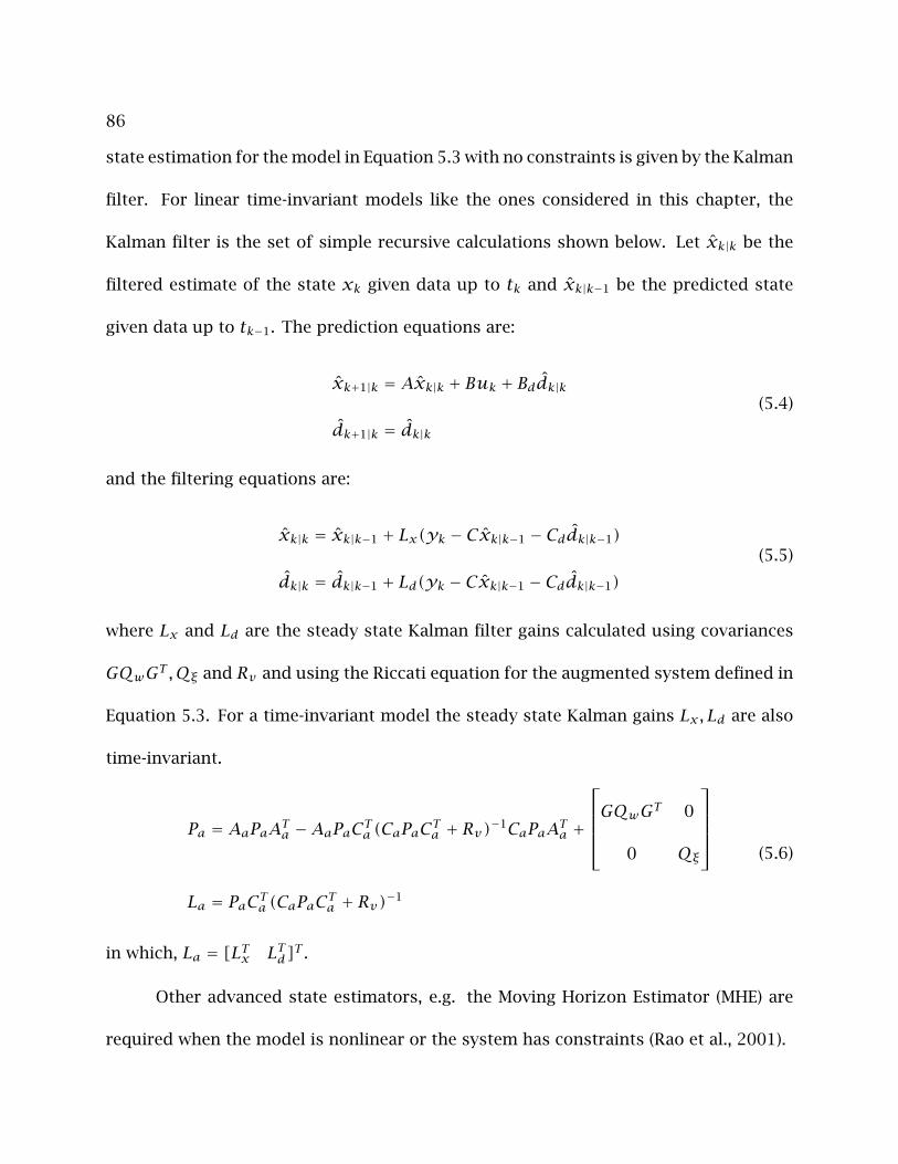
86

state estimation for the model in Equation 5.3 with no constraints is given by the Kalman

filter. For linear time-invariant models like the ones considered in this chapter, the

Kalman filter is the set of simple recursive calculations shown below. Let xk|k be the

filtered estimate of the state xk given data up to tk and xk|k−1 be the predicted state

given data up to tk−1. The prediction equations are:

xk+1|k = Axk|k + Buk + Bddk|k

dk+1|k = dk|k(5.4)

and the filtering equations are:

xk|k = xk|k−1 + Lx(yk − Cxk|k−1 − Cddk|k−1)

dk|k = dk|k−1 + Ld(yk − Cxk|k−1 − Cddk|k−1)(5.5)

where Lx and Ld are the steady state Kalman filter gains calculated using covariances

GQwGT ,Qξ and Rv and using the Riccati equation for the augmented system defined in

Equation 5.3. For a time-invariant model the steady state Kalman gains Lx, Ld are also

time-invariant.

Pa = AaPaATa −AaPaCTa (CaPaCTa + Rv)−1CaPaATa +

GQwGT 0

0 Qξ

La = PaCTa (CaPaCTa + Rv)−1

(5.6)

in which, La = [LTx LTd]T .

Other advanced state estimators, e.g. the Moving Horizon Estimator (MHE) are

required when the model is nonlinear or the system has constraints (Rao et al., 2001).

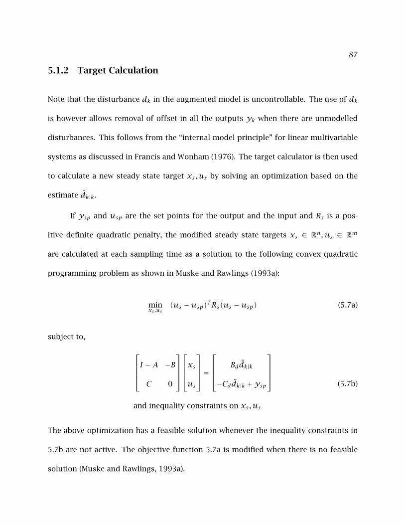
87

5.1.2 Target Calculation

Note that the disturbance dk in the augmented model is uncontrollable. The use of dk

is however allows removal of offset in all the outputs yk when there are unmodelled

disturbances. This follows from the “internal model principle” for linear multivariable

systems as discussed in Francis and Wonham (1976). The target calculator is then used

to calculate a new steady state target xs , us by solving an optimization based on the

estimate dk|k.

If ysp and usp are the set points for the output and the input and Rs is a pos-

itive definite quadratic penalty, the modified steady state targets xs ∈ Rn, us ∈ Rm

are calculated at each sampling time as a solution to the following convex quadratic

programming problem as shown in Muske and Rawlings (1993a):

minxs ,us

(us −usp)TRs(us −usp) (5.7a)

subject to,

I −A −B

C 0

xsus

= Bddk|k

−Cddk|k +ysp

and inequality constraints on xs , us

(5.7b)

The above optimization has a feasible solution whenever the inequality constraints in

5.7b are not active. The objective function 5.7a is modified when there is no feasible

solution (Muske and Rawlings, 1993a).

88

5.1.3 Regulation

The receding horizon formulation for the regulator in MPC is given as the quadratic

objective function with the model constraints and penalties Q ≥ 0, R ≥ 0. The state

and the input are penalized for deviations from the steady state targets calculated from

Equation 5.7a (Muske and Rawlings, 1993a).

minuk,··· ,uk+Nc

k+Nc∑j=k(xj|k − xs)TQ(xj|k − xs)+ (uj −us)TR(uj −us)

subject to, xj+1|k = Axj|k + Buj + Bddk|k, j ≥ k

(5.8)

The state and input constraints are not shown in the above formulation for ease of

notation. Inclusion of the constraints do not change any of the analysis that follows.

Here, the control horizon and the prediction horizon are taken to be the same: Nc .

Assuming that the filtered disturbance dk|k remains unchanged over the future hori-

zon Nc and the current state taken as the estimate xk|k, the optimized control moves

u∗k , u∗k+1, · · ·u∗k+Nc over the horizon are calculated and only the first move u∗k is im-

plemented at time tk.

The estimation, target calculation and regulation is repeated at every time step.

For Nc → ∞ and no constraints on input and state, the optimization in Equation 5.8 is

equivalent to the Linear Quadratic Regulator (LQR).

Remark 5.1. Note that the state estimation in Section 5.1.1 requires knowledge of the co-

variances GQwGT ,Qξ, Rv and the target calculation in Section 5.1.2 requires the struc-

ture of the unmodelled disturbances given by the matrices Bd, Cd. In general, none of

89

these are known from first principles modelling. The ideal choice of Bd, Cd is one that rep-

resents the unmodelled disturbance in the plant accurately. The choice of the disturbance

model has been the subject of research (Lee et al., 1994; Pannocchia, 2003; Eppler, 1997;

Shinskey, 1994, chap. 5). These studies assume that the covariances GQwGT ,Qξ, Rv are

known and the models Bd, Cd are unknown. However in Sections 5.3 and 5.4 we show

that if an incorrect choice for Bd, Cd is made, then the covariances GQwGT ,Qξ, Rv esti-

mated from data are within an equivalent transformation such that the particular choice

of Bd, Cd has no effect on the closed-loop performance.

5.2 Motivation

The rules for choosing the penalties Q,R for the regulator are well researched and

based on intuitive reasoning (see for example Anderson and Moore (1990, chap. 6)).

The estimator on the other hand requires knowledge of the disturbance covariances

GQwGT , Rv ,Qξ and the disturbance models Bd, Cd. Consider an unconstrained single

input single output plant with the following values for the parameters:

A = 0.5, B = 0.5, C = 1, ysp = 0.8

Let a deterministic unmodelled disturbance of magnitude 1 enter the input at sampling

time 3 and is measured at sampling time 4. Let there be no other noises affecting the

plant: GQwGT = 0, Rv = 0. An incorrect choice of the MPC disturbance model would

be Bd = 0, Cd = 1 modelling the disturbance as entering at the output. The actual plant

90

model on the other hand is Bd = B = 0.5, Cd = 0 (the input disturbance model).

We now compare the closed-loop performance for the incorrect disturbance model

against the plant disturbance model. The regulator is chosen to be the LQR with penal-

ties Q = 1, R = 0 and penalty Rs = 1 for the target calculator. If the covariances

GQwGT ,Qξ, Rv were assumed to be known then the optimal state estimator is the

deadbeat Kalman filter gain for the input disturbance model calculated by substitut-

ing GQwGT = 0, Rv ≈ 0,Qξ 6= 0 in the Kalman filter Equation 5.6. The deadbeat Kalman

gains for the input disturbance model is L1 =

1

2

and for the incorrect output dis-

turbance model is L2 =

0

1

. The control law is the same both cases and given by the

LQR feedback: uk = K(xk|k − xs). The rejection of the deterministic disturbance in the

two cases is show in Figure 5.3. With the input disturbance model, the disturbance in

the input is estimated and rejected much more quickly than when using the incorrect

model although the same covariancesGQwGT , Rv ,Qξ are used in the calculation of both

the state estimators. The sluggish behavior of the output disturbance model and the

decrease in closed-loop performance is due to the choice of the disturbance model and

the chosen estimator gain. A similar difference in the performance with the incorrect

choice of the disturbance model was noted by Shinskey (1994, chap. 5); Lee et al. (1994);

Muske and Rawlings (1993b); Muske and Badgwell (2002).

Since we usually lack knowledge about the structure of the unmodelled distur-

bances (matrices Bd, Cd), the only other handle to change the input-output performance

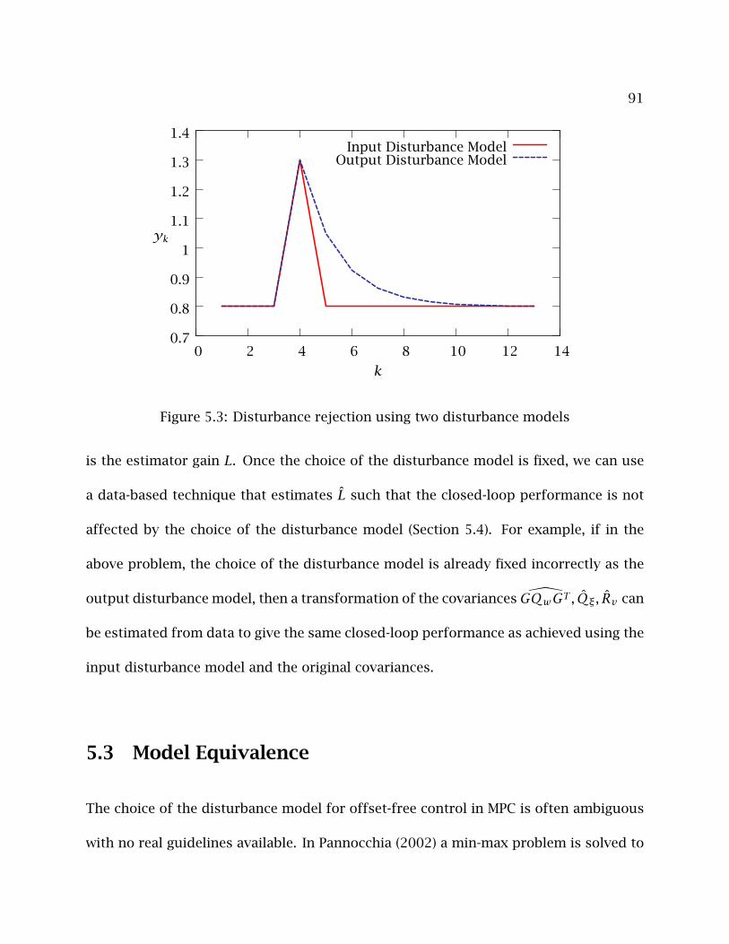
91

0.7

0.8

0.9

1

1.1

1.2

1.3

1.4

0 2 4 6 8 10 12 14

k

yk

Input Disturbance ModelOutput Disturbance Model

Figure 5.3: Disturbance rejection using two disturbance models

is the estimator gain L. Once the choice of the disturbance model is fixed, we can use

a data-based technique that estimates L such that the closed-loop performance is not

affected by the choice of the disturbance model (Section 5.4). For example, if in the

above problem, the choice of the disturbance model is already fixed incorrectly as the

output disturbance model, then a transformation of the covariances GQwGT , Qξ, Rv can

be estimated from data to give the same closed-loop performance as achieved using the

input disturbance model and the original covariances.

5.3 Model Equivalence

The choice of the disturbance model for offset-free control in MPC is often ambiguous

with no real guidelines available. In Pannocchia (2002) a min-max problem is solved to

92

find the best performing disturbance model. Most industrial MPC implementations such

as IDCOM (Richalet et al., 1978), DMC (Cutler and Ramaker, 1980) and QDMC (Garcıa

and Morshedi, 1986) use an output disturbance model to remove offset . The choice

of the output disturbance model has been criticized in the literature as being sluggish

in rejecting disturbances (Shinskey, 1994, chap. 5),(Lee et al., 1994). In this section we

show that for linear time-invariant (LTI) systems, disturbance models are equivalent as

long as the estimator is determined with the appropriate covariances.

Remark 5.2. It is interesting to examine some of the early history of disturbance mod-

elling. Box and Jenkins clearly make the point that one can identify equivalent distur-

bance models that represent different disturbance sources by what they call “transfer of

disturbance origins.” (Box and Jenkins, 1970, p. 469, 1st edition). Note that the inter-

ested reader must obtain the first edition because by the 3rd edition (Box et al., 1994), this

terminology and entire discussion had been deleted. Box and Jenkins also point out that

identifying a disturbance model with data collected in a fashion that does not include all

relevant disturbances that are encountered in closed-loop operation does not produce an

optimal control because the disturbance model consequently has significant error. They

recommend using closed-loop identification (Box and Jenkins, 1970, p. 471, 1st ed) to

avoid the accidental neglect of disturbance sources.

In this work, we are emphasizing again Box and Jenkins’s conclusion that one is

free to choose the source of the disturbance in the disturbance model, and one naturally

requires data that include all relevant disturbances. It is irrelevant, however, if these data

93

are collected under closed-loop or open-loop control. Also, we are not interested in iden-

tifying the disturbance model, which was the primary focus of Box and Jenkins’s earlier

work. We fully expect the practitioner to employ an integrated white noise disturbance

model to represent essentially all of the plant disturbances. The motivation is to remove

steady offset in the closed-loop system output, not to capture an accurate dynamic model

of the true disturbance. A contribution of the current chapter therefore is to propose

and show that such rough disturbance models are often completely adequate to handle

disturbances entering from other sources with different dynamics, if one estimates the

statistics of the driving noise from data.

Consider two choices of the disturbance models (Bd1, Cd1) and (Bd2, Cd2) satis-

fying detectability conditions. If nd is the dimension of the disturbance vector, the

assumption of detectability implies (Pannocchia and Rawlings, 2002):

rank

A− I Bd1

C Cd1

= n+nd, rank

A− I Bd2

C Cd2

= n+nd (5.9)

Note that if the disturbance in the actual plant is not detectable, then the state estimator

is defined for a transformed, lower dimensional model that is detectable.

The systems augmented with the disturbance model are simple nonminimal re-

alizations of the same unaugmented model where dk is an uncontrollable state. The

augmented systems with the two general disturbance models can be written as follows:

94

Model 1: x1

d1

k+1

=

A Bd1

0 I

︸︷︷︸

A1

x1

d1

k

+

B0

︸︷︷︸Ba

uk +G1

wξ

k

yk =[C Cd1

]︸︷︷︸

C1

x1

d1

k

+ vk

(5.10)

Model 2: x2

d2

k+1

=

A Bd2

0 I

︸︷︷︸

A2

x2

d2

k

+

B0

︸︷︷︸Ba

uk +G2

wξ

k

yk =[C Cd2

]︸︷︷︸

C2

x2

d2

k

+ vk

(5.11)

If the two models have the same input to output relationship, there exists a similarity

transformation matrix T such that:

TA1T−1 = A2, C1T−1 = C2, TBa = Ba (5.12)

Also for Models 1 and 2 the unknown stochastic parameters G1 and G2 must satisfy:

TG1 = G2 (5.13)

Lemma 5.1. If the augmented models in Equations 5.10 and 5.11 are assumed to be de-

tectable, then the transformation relations in Equation 5.12 can be expressed equivalently

95

as:

T11 = I,

A− I Bd2

C Cd2

T12

T22

=Bd1

Cd1

, T21 = 0

where, T is partitioned as (with appropriate dimensions):

T =

T11 T12

T21 T22

Proof. The proof is given in Appendix 5.7.1

Theorem 5.1. For the two detectable augmented models in Equations 5.10 and 5.11, a

transformation matrix T satisfying the relations in Equation 5.12 exists and is unique if

and only if the following condition holds:

rank

A− I Bd1 Bd2

C Cd1 Cd2

= n+nd (5.14)

Proof. The proof follows from the relations in Equation 5.12 expressed equivalently

from Lemma 5.1 and the detectability conditions in Equation 5.9.

Note that for zero offset in all the outputs yk, we need nd = p. The condition in

Theorem 5.1 is then automatically satisfied for all detectable disturbance models.

Remark 5.3. Notice that we are considering a known and fixed minimal input-output

realization of the triple (A, B,C). The LQR cost in Equation 5.8 then remains unchanged

for the two nonminimal augmented models in Equations 5.10 and 5.11 related by the

conditions given in Lemma 5.1.

96

An alternate derivation and condition for the transformation matrix in Equation

5.12 is given in Appendix 5.7.3.

5.3.1 Special Case of Equivalence

For an input disturbance model we have Bd = B and Cd = 0 and for an output distur-

bance model we have Bd = 0 and Cd = I. For these particular choices of the disturbance

models with nd =m = p, we get the following transformation matrix:

• Model 1- Bd1 = B,Cd1 = 0, Model 2-Bd2 = 0, Cd2 = I

T =

I (A− I)−1B

0 −C(A− I)−1B

(5.15)

Remark 5.4. Note that when A has an integrator, the inverses above are not defined. In

this case the output disturbance model is not detectable and fails Theorem 5.1. This has

been long known in the literature as a potential problem with industrial MPC implementa-

tions such as IDCOM, DMC, QDMC, which use a constant output step disturbance model

(Morari and Lee, 1991; Muske and Badgwell, 2002; Qin and Badgwell, 2003). Various

fixes have also been suggested in the literature by Marquis and Broustail (1988); Li et al.

(1989); Lundstrom et al. (1995); Gupta (1998) and Dougherty and Cooper (2003).

5.3.2 Equivalent Closed-loop Performance

Given Models 1 and 2 related by the equivalence transformation matrix T satisfying

the relations in Equation 5.12, from realization theory (Ho and Kalman, 1966) equiv-

97

alent closed-loop performance for the two models implies that given a sequence of

control actions u1, · · · , uk−1 and noise sequences w1, · · · ,wk−1, ξ1, · · ·ξk−1 and

v1, · · · , vk, then the output sequence from the two models: y1, · · · , yk are the

same starting from zero initial conditions. When these models are used in MPC, the

noises wk, ξk, vk are unknown.

If L1 and L2 are the state estimator gains (not necessarily the Kalman filter gains)

for Models 1 and 2, then equivalent closed-loop performance implies that given the in-

puts u1, · · · , uk−1 and outputs y1, · · · , yk, the innovations sequence Y1, · · · ,Yk

are the same, where Yk = (yk − yk|k−1). The innovations for the augmented system in

Equation 5.3 are given by Equations 5.4 and 5.5:xd

k+1|k

= Aa

xd

k|k−1

+ Bauk +AaLa(yk − yk|k−1)

Yk = yk − Ca

xd

k|k−1

(5.16)

Lemma 5.2. Given a set of measurements y1, · · · , yk and inputs u1, · · · , uk−1 and

the two disturbance models in Equations 5.10 and 5.11 related to each other through

the unique transformation matrix T satisfying Equation 5.12, the innovations sequence

defined as Yk = (yk − yk|k−1) are the same for the two models if and only if the state

estimator gains (can be suboptimal gains) satisfy the relation:

L2 = TL1 (5.17)

Proof. The proof follows using simple algebraic manipulations using Equations 5.10

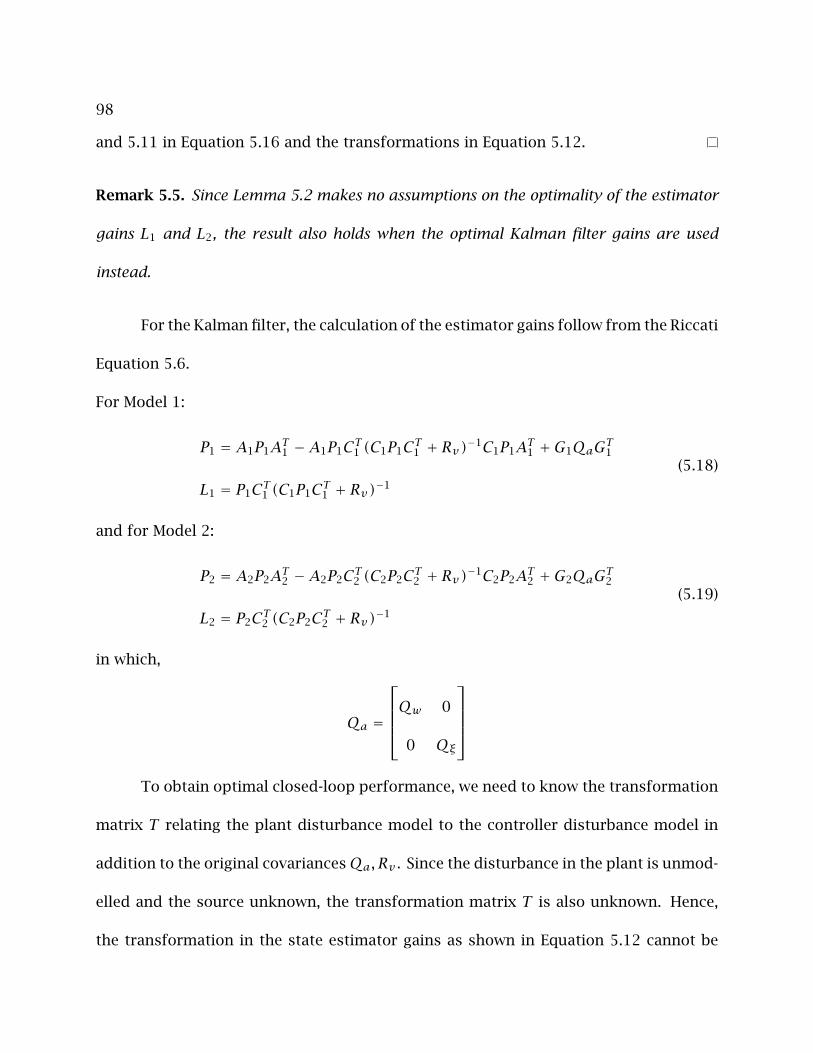
98

and 5.11 in Equation 5.16 and the transformations in Equation 5.12.

Remark 5.5. Since Lemma 5.2 makes no assumptions on the optimality of the estimator

gains L1 and L2, the result also holds when the optimal Kalman filter gains are used

instead.

For the Kalman filter, the calculation of the estimator gains follow from the Riccati

Equation 5.6.

For Model 1:

P1 = A1P1AT1 −A1P1CT1 (C1P1CT1 + Rv)−1C1P1AT1 +G1QaGT1

L1 = P1CT1 (C1P1CT1 + Rv)−1

(5.18)

and for Model 2:

P2 = A2P2AT2 −A2P2CT2 (C2P2CT2 + Rv)−1C2P2AT2 +G2QaGT2

L2 = P2CT2 (C2P2CT2 + Rv)−1

(5.19)

in which,

Qa =

Qw 0

0 Qξ

To obtain optimal closed-loop performance, we need to know the transformation

matrix T relating the plant disturbance model to the controller disturbance model in

addition to the original covariancesQa, Rv . Since the disturbance in the plant is unmod-

elled and the source unknown, the transformation matrix T is also unknown. Hence,

the transformation in the state estimator gains as shown in Equation 5.12 cannot be

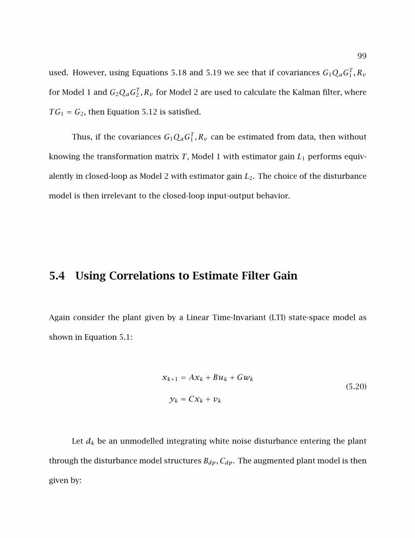
99

used. However, using Equations 5.18 and 5.19 we see that if covariances G1QaGT1 , Rv

for Model 1 and G2QaGT2 , Rv for Model 2 are used to calculate the Kalman filter, where

TG1 = G2, then Equation 5.12 is satisfied.

Thus, if the covariances G1QaGT1 , Rv can be estimated from data, then without

knowing the transformation matrix T , Model 1 with estimator gain L1 performs equiv-

alently in closed-loop as Model 2 with estimator gain L2. The choice of the disturbance

model is then irrelevant to the closed-loop input-output behavior.

5.4 Using Correlations to Estimate Filter Gain

Again consider the plant given by a Linear Time-Invariant (LTI) state-space model as

shown in Equation 5.1:


yk = Cxk + vk(5.20)

Let dk be an unmodelled integrating white noise disturbance entering the plant

through the disturbance model structures Bdp, Cdp. The augmented plant model is then

given by:

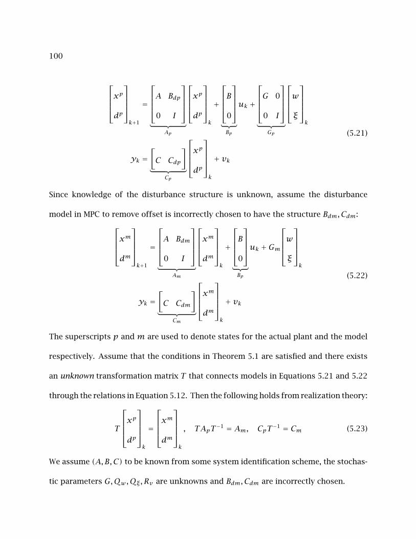
100

xp

dp

k+1

=

A Bdp

0 I

︸︷︷︸

Ap

xp

dp

k

+

B0

︸︷︷︸Bp

uk +

G 0

0 I

︸︷︷︸

Gp

wξ

k

yk =[C Cdp

]︸︷︷︸

Cp

xp

dp

k

+ vk

(5.21)

Since knowledge of the disturbance structure is unknown, assume the disturbance

model in MPC to remove offset is incorrectly chosen to have the structure Bdm, Cdm:xm

dm

k+1

=

A Bdm

0 I

︸︷︷︸

Am

xm

dm

k

+

B0

︸︷︷︸Bp

uk +Gm

wξ

k

yk =[C Cdm

]︸︷︷︸

Cm

xm

dm

k

+ vk

(5.22)

The superscripts p and m are used to denote states for the actual plant and the model

respectively. Assume that the conditions in Theorem 5.1 are satisfied and there exists

an unknown transformation matrix T that connects models in Equations 5.21 and 5.22

through the relations in Equation 5.12. Then the following holds from realization theory:

T

xp

dp

k

=

xm

dm

k

, TApT−1 = Am, CpT−1 = Cm (5.23)

We assume (A, B,C) to be known from some system identification scheme, the stochas-

tic parameters G,Qw ,Qξ, Rv are unknowns and Bdm, Cdm are incorrectly chosen.

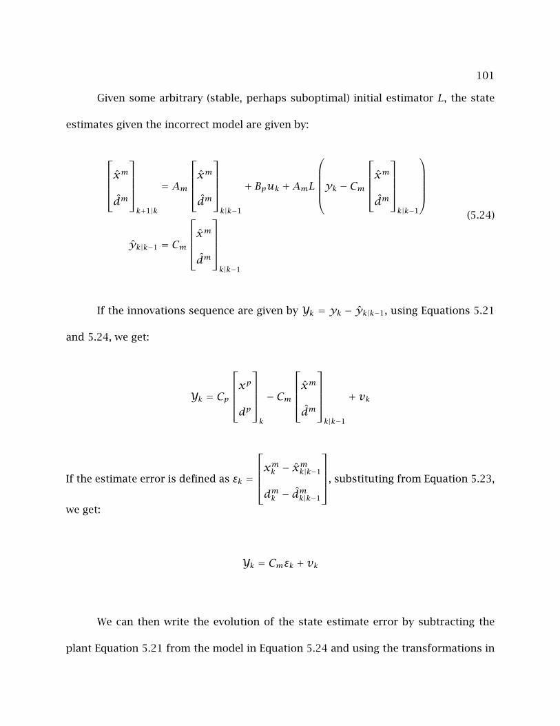
101

Given some arbitrary (stable, perhaps suboptimal) initial estimator L, the state

estimates given the incorrect model are given by:

xm

dm

k+1|k

= Am

xm

dm

k|k−1

+ Bpuk +AmL

yk − Cmx

m

dm

k|k−1

yk|k−1 = Cm

xm

dm

k|k−1

(5.24)

If the innovations sequence are given by Yk = yk − yk|k−1, using Equations 5.21

and 5.24, we get:

Yk = Cp

xp

dp

k

− Cm

xm

dm

k|k−1

+ vk

If the estimate error is defined as εk =

xmk − xmk|k−1

dmk − dmk|k−1

, substituting from Equation 5.23,

we get:

Yk = Cmεk + vk

We can then write the evolution of the state estimate error by subtracting the

plant Equation 5.21 from the model in Equation 5.24 and using the transformations in

102

Equation 5.23:

εk+1 = (Am −AmLCm)︸︷︷︸A

εk +[TGp −AmL

]︸︷︷︸

G

w

ξ

v

k

Yk = Cmεk + vk

(5.25)

We define the autocovariance as Cj = E[YkYTk+j], the expectation of data at dif-

ferent time lags Jenkins and Watts (1968, p. 146). Using Equation 5.25 we can write the

following expectation of covariances:

E[YkYTk ] = CmPCTm + Rv (5.26)

E[Yk+jYTk ] = CmAjPCTm − CmAj−1AmLRv j ≥ 1 (5.27)

which are independent of k when we assume that data are collected when operating

at steady state. Again using Equation 5.25 we note that P = E[εkεTk ] the steady state

estimate error covariance satisfies the Lyapunov equation:

P = APAT +[TGp −AmL

]︸︷︷︸

G

Qa 0

0 Rv

GT where, Qa =

Qw 0

0 Qξ

(5.28)

A computation of the first column block of the Autocovariance Matrix of inno-

vations process over some user defined window N then gives (Chapter 3 and Odelson

103

et al. (2006b)):

R1(N) =

C0

C1

...

CN−1

=

Cm

CmA

...

CmAN−1

︸︷︷︸

O

PCTm +

I

−CmAmL...

−CmAN−2AmL

︸︷︷︸

Γ

Rv (5.29)

Define the following covariance product:

Q Õ TGpQaGTpT T

Notice that in the above Equation 5.29 with P given by Equation 5.28, the only unknowns

are the transformed covarianceQ and Rv . If R1(N) is an estimate ofR1(N) from data,

then similar to the development of the ALS technique in Chapter 3, we can express

Equation 5.29 as a weighted least-squares problem in a vector of unknowns (Q)s , (Rv)s .

Here, the subscript ‘s’ denotes the column-wise stacking of the elements of the matrix

in a vector. As before, we add semidefinite constraints to ensure the covariances to be

positive semidefinite. We then get the following convex autocovariance least-squares

(ALS) optimization problem developed in Chapter 3:

Φ =minQ,Rv

∥∥∥∥∥∥∥∥∥A (Q)s(Rv)s

− b∥∥∥∥∥∥∥∥∥

2

W

subject to, Q ≥ 0, Rv ≥ 0, Q = QT , Rv = RTv

(5.30)

104

whereA is defined from Chapter 3 as,

A=[A1 A2]

A1 =[(C ⊗O)(In2 − A⊗ A)−1]

A2 =[(C ⊗O)(In2 − A⊗ A)−1(AL⊗AL)+ (Ip ⊗ Γ)]

(5.31)

Theorem 5.2. IfA has full column rank then in the limit of large data: Nd →∞, whereNd

is the length of the innovations sequence used to estimate R1(N), the ALS technique gives

unbiased estimates for the covariances: limNd→∞ Q → TGpQaGTpT T and limNd→∞ Rv →

Rv .

Proof. See Odelson et al. (2006b) for proof showing that the estimates are unbiased.

Lemma 5.3. If covariances TGpQaGTpT T andRv are used to calculate the Kalman filter for

the incorrect disturbance model in Equation 5.22, then the resulting innovations sequence

is the same as when using the optimal Kalman filter with the actual plant disturbance

model in Equation 5.21.

Proof. Substituting TGpQaGTpT T and Rv in the Kalman filter Equation 5.6 for the incor-

rect model in Equation 5.22 and using the transformations in Equation 5.23, we get:

Lm = TLp

Equivalence and optimality of the innovations sequence then follows from Lemma 5.2

and noting that Lm is the optimal Kalman gain for the disturbance model in Equation

5.21.

105

Thus, even when the disturbance model is chosen different from the actual plant

disturbance location, the ALS technique can be used to estimate transformed covari-

ances such that the closed-loop performance is equivalent to that achieved using the

optimal filter and the actual plant disturbance model.

Necessary and sufficient conditions for uniqueness of the ALS problem in Equa-

tion 5.30 are given by Theorem 3.1 in Chapter 3. Its informative to note that A in

Equation 5.30 may not be full rank giving nonunique estimates to the ALS optimization.

The nonuniqueness however, is not a limitation as shown in Theorem 5.3.

Theorem 5.3. Given that the ALS optimization in Equation 5.30 is not unique, every

nonunique solution gives the same Kalman filter gain.

Proof. From Lemma 3.1 in Chapter 3, since the ALS optimization is not unique the matrix

A defined in Equation 5.31 is not full column rank.

In addition from the statement and the proof to Lemma 3.2 in Chapter 3 we have

the following condition:

(C ⊗ In)(In2 − (A⊗ A))−1Dna(QN)ss = 0 (5.32)

where, na is the dimension ofQ and

(QN)ss0

is an element in the null space of theA.

The subscript ‘ss’ denotes the column-wise stacking of only the symmetric elements of

the matrix QN . Define PN uniquely as: (PN)s = (In2 − A ⊗ A)−1Dna(QN)ss . Notice that

restacking the above vectors column-wise into a matrix and using rules of Kronecker

106

products gives the following Lyapunov Equation:

PN = APNAT +QN

Also from Equation 5.32, we see that PN is symmetric and satisfies

PNCT = 0, CPN = 0 (5.33)

giving:

PN = APNAT +QN (5.34)

Let Q, Rv be estimates from the ALS optimization. From the proof of Lemma 3.2 we

have that Rv is a unique estimate and Q is any arbitrary nonunique estimate. Also, every

nonunique estimate of Q is characterized by Q+αQN where α is a scalar, provided the

sum is positive semidefinite.

Let the Kalman filter gain using the above estimates be L calculated as:

P = AmPATm −AmPCTm(CmPCTm + Rv)−1CmPATm + Q

L = PCTm(CmPCTm + Rv)−1

(5.35)

If we define P = P + αPN and Q = Q + αQN , then using Equations 5.33 and 5.34, we

see that P and Q can be substituted in Equation 5.35 to produce the same Kalman filter

gain L. Thus, the statement in this theorem is proved.

5.5 Simulation Examples

The following examples illustrate the ideas developed in the previous sections. Closed-

loop performance of a pure input disturbance model (Bd = B,Cd = 0) is compared

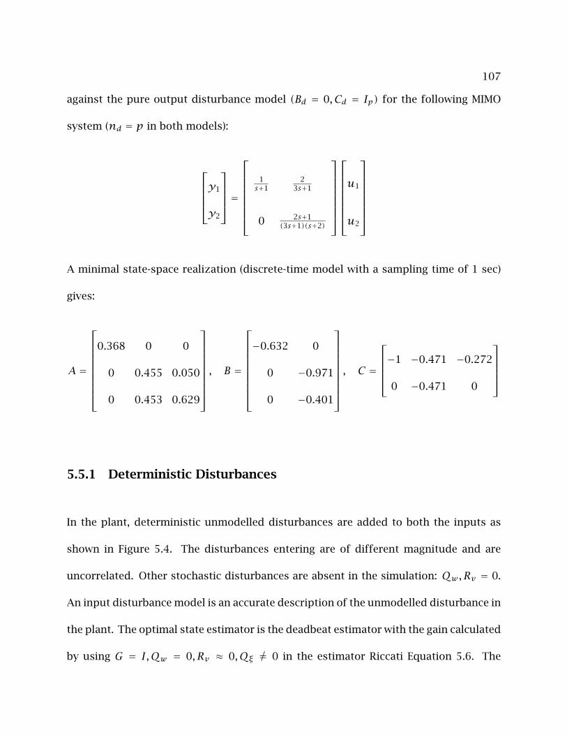
107

against the pure output disturbance model (Bd = 0, Cd = Ip) for the following MIMO

system (nd = p in both models):

y1

y2

=

1s+1

23s+1

0 2s+1(3s+1)(s+2)

u1

u2

A minimal state-space realization (discrete-time model with a sampling time of 1 sec)

gives:

A =

0.368 0 0

0 0.455 0.050

0 0.453 0.629

, B =

−0.632 0

0 −0.971

0 −0.401

, C =

−1 −0.471 −0.272

0 −0.471 0

5.5.1 Deterministic Disturbances

In the plant, deterministic unmodelled disturbances are added to both the inputs as

shown in Figure 5.4. The disturbances entering are of different magnitude and are

uncorrelated. Other stochastic disturbances are absent in the simulation: Qw , Rv = 0.

An input disturbance model is an accurate description of the unmodelled disturbance in

the plant. The optimal state estimator is the deadbeat estimator with the gain calculated

by using G = I,Qw = 0, Rv ≈ 0,Qξ 6= 0 in the estimator Riccati Equation 5.6. The

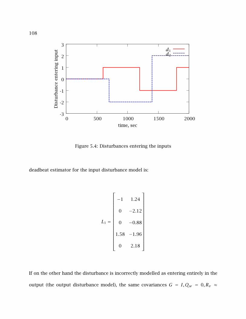
108

-3

-2

-1

0

1

2

3

0 500 1000 1500 2000

Dis

turb

ance

ente

rin

gin

pu

t

time, sec

d1d2

Figure 5.4: Disturbances entering the inputs

deadbeat estimator for the input disturbance model is:

L1 =

−1 1.24

0 −2.12

0 −0.88

1.58 −1.96

0 2.18

If on the other hand the disturbance is incorrectly modelled as entering entirely in the

output (the output disturbance model), the same covariances G = I,Qw = 0, Rv ≈

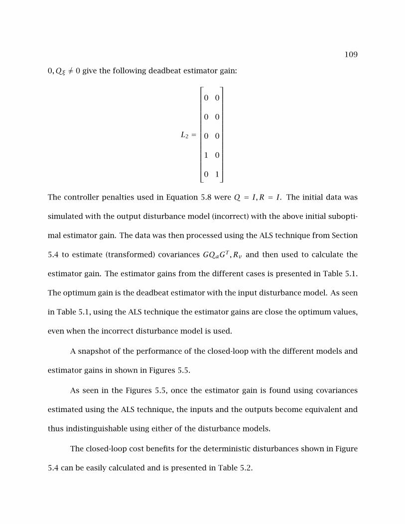
109

0,Qξ 6= 0 give the following deadbeat estimator gain:

L2 =

0 0

0 0

0 0

1 0

0 1

The controller penalties used in Equation 5.8 were Q = I, R = I. The initial data was

simulated with the output disturbance model (incorrect) with the above initial subopti-

mal estimator gain. The data was then processed using the ALS technique from Section

5.4 to estimate (transformed) covariances GQaGT , Rv and then used to calculate the

estimator gain. The estimator gains from the different cases is presented in Table 5.1.

The optimum gain is the deadbeat estimator with the input disturbance model. As seen

in Table 5.1, using the ALS technique the estimator gains are close the optimum values,

even when the incorrect disturbance model is used.

A snapshot of the performance of the closed-loop with the different models and

estimator gains in shown in Figures 5.5.

As seen in the Figures 5.5, once the estimator gain is found using covariances

estimated using the ALS technique, the inputs and the outputs become equivalent and

thus indistinguishable using either of the disturbance models.

The closed-loop cost benefits for the deterministic disturbances shown in Figure

5.4 can be easily calculated and is presented in Table 5.2.

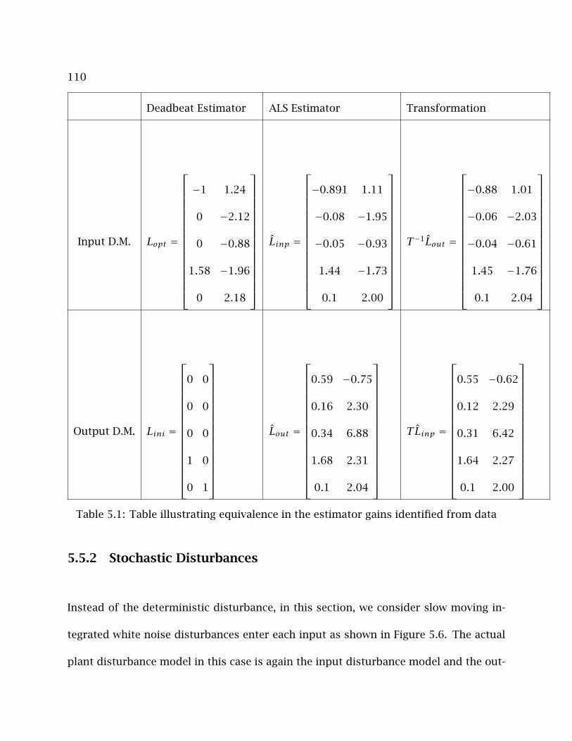
110

Deadbeat Estimator ALS Estimator Transformation

Input D.M. Lopt =

−1 1.24

0 −2.12

0 −0.88

1.58 −1.96

0 2.18

Linp =

−0.891 1.11

−0.08 −1.95

−0.05 −0.93

1.44 −1.73

0.1 2.00

T−1Lout =

−0.88 1.01

−0.06 −2.03

−0.04 −0.61

1.45 −1.76

0.1 2.04

Output D.M. Lini =

0 0

0 0

0 0

1 0

0 1

Lout =

0.59 −0.75

0.16 2.30

0.34 6.88

1.68 2.31

0.1 2.04

TLinp =

0.55 −0.62

0.12 2.29

0.31 6.42

1.64 2.27

0.1 2.00

Table 5.1: Table illustrating equivalence in the estimator gains identified from data

5.5.2 Stochastic Disturbances

Instead of the deterministic disturbance, in this section, we consider slow moving in-

tegrated white noise disturbances enter each input as shown in Figure 5.6. The actual

plant disturbance model in this case is again the input disturbance model and the out-

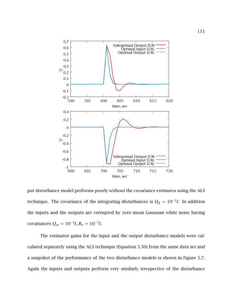
111

-0.2

-0.1

0

0.1

0.2

0.3

0.4

0.5

0.6

0.7

590 595 600 605 610 615 620

time, sec

y1

Suboptimal Output D.MOptimal Input D.M.

Optimal Output D.M.

-1

-0.8

-0.6

-0.4

-0.2

0

0.2

0.4

690 695 700 705 710 715 720

time, sec

y2

Suboptimal Output D.MOptimal Input D.M.

Optimal Output D.M.

put disturbance model performs poorly without the covariance estimates using the ALS

technique. The covariance of the integrating disturbances is Qξ = 10−3I. In addition

the inputs and the outputs are corrupted by zero mean Gaussian white noise having

covariances Qw = 10−4I, Rv = 10−5I.

The estimator gains for the input and the output disturbance models were cal-

culated separately using the ALS technique (Equation 5.30) from the same data set and

a snapshot of the performance of the two disturbance models is shown in Figure 5.7.

Again the inputs and outputs perform very similarly irrespective of the disturbance

112

-1.4

-1.2

-1

-0.8

-0.6

-0.4

-0.2

0

0.2

590 595 600 605 610 615 620

time, sec

u1

Suboptimal Output D.M.Optimal Input D.M.

Optimal Output D.M.

-0.5

0

0.5

1

1.5

2

2.5

3

690 695 700 705 710 715 720

time, sec

u2

Suboptimal Output D.M.Optimal Input D.M.

Optimal Output D.M.

Figure 5.5: Closed-loop performance using estimator gains from the ALS technique

(D.M.=Disturbance Model)

model chosen once the ALS technique is used to calculate the estimator gains.

The comparison between the expected closed-loop costs (see Appendix 5.7.2 for

calculation of closed-loop cost) for the three cases is presented in Table 5.3. Note that

the optimal closed-loop cost is 1.788× 10−4.

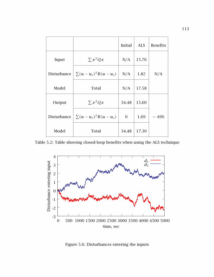
113

Initial ALS Benefits

Input∑xTQx N/A 15.76

Disturbance∑(u−us)TR(u−us) N/A 1.82 N/A

Model Total N/A 17.58

Output∑xTQx 34.48 15.60

Disturbance∑(u−us)TR(u−us) 0 1.69 ∼ 49%

Model Total 34.48 17.30

Table 5.2: Table showing closed-loop benefits when using the ALS technique

-3

-2

-1

0

1

2

3

4

0 500 1000 1500 2000 2500 3000 3500 4000 4500 5000

Dis

turb

ance

ente

rin

gin

pu

t

time, sec

d1d2

Figure 5.6: Disturbances entering the inputs

114

-0.15

-0.1

-0.05

0

0.05

0.1

0.15

590 595 600 605 610 615 620

time, sec

y1

Suboptimal Output D.MOptimal Input D.M.Optimal Output D.M.

-0.03

-0.02

-0.01

0

0.01

0.02

0.03

690 695 700 705 710 715 720

time, sec

y2

Suboptimal Output D.MOptimal Input D.M.Optimal Output D.M.

Stochastic Closed-loop Cost Initial (×104) ALS (×104) Benefits

Input D.M. E[xTkQxk +uTkRuk] N/A 1.817 N/A

Output D.M. E[xTkQxk +uTkRuk] 5.659 1.897 66.5%

Table 5.3: Table showing expectation of closed-loop cost for different estimator gains

(Optimal Cost is 1.788× 10−4). See Appendix 5.7.2.

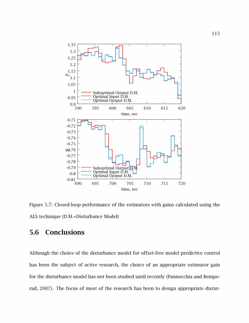
115

0.9

0.95

1

1.05

1.1

1.15

1.2

1.25

1.3

1.35

590 595 600 605 610 615 620

time, sec

u1

Suboptimal Output D.M.Optimal Input D.M.Optimal Output D.M.

-0.81

-0.8

-0.79

-0.78

-0.77

-0.76

-0.75

-0.74

-0.73

-0.72

-0.71

690 695 700 705 710 715 720

time, sec

u2

Suboptimal Output D.M.Optimal Input D.M.Optimal Output D.M.

Figure 5.7: Closed-loop performance of the estimators with gains calculated using the

ALS technique (D.M.=Disturbance Model)

5.6 Conclusions

Although the choice of the disturbance model for offset-free model predictive control

has been the subject of active research, the choice of an appropriate estimator gain

for the disturbance model has not been studied until recently (Pannocchia and Bempo-

rad, 2007). The focus of most of the research has been to design appropriate distur-

116

bance models to accurately represent the actual plant disturbance source while assum-

ing that the estimator gain is known. In Section 5.3 it was shown that since different

augmented disturbance models are nonminimal realizations of the same input-output

process, there exists estimator gain matrices for each disturbance model that achieve

the same closed-loop input-output performance.

In Section 5.4 an autocovariance least-squares (ALS) technique was presented to

estimate the covariances of the disturbance model from steady state data (closed-loop

or open-loop) irrespective of the true disturbance source. The estimation of these co-

variances and hence the estimator gain was shown to compensate automatically for the

incorrect choice of the model’s disturbance location. Examples were presented to show

the benefits of using the ALS technique to estimate the covariances and to illustrate the

equivalent closed-loop performance using different disturbance models.

A direct implication of the results presented in this chapter is that an industrial

practitioner can model the disturbance as an integrator at any location in the plant but

then use the autocovariance of the data to estimate the disturbance covariances to cal-

culate the estimator gain. The control performance using this rough disturbance model

and data-based estimator gain is often comparable to that obtained using a disturbance

model that accurately represents the true plant disturbance. Modeling effort can then

be directed to obtaining the estimator gain from data rather than trying to model ac-

curately the dynamics of the unknown disturbance, which is a much more complex

modeling task.

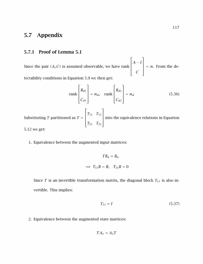
117

5.7 Appendix


Since the pair (A,C) is assumed observable, we have rank

A− IC

= n. From the de-

tectability conditions in Equation 5.9 we then get:

rank

Bd1

Cd1

= nd, rank

Bd2

Cd2

= nd (5.36)

Substituting T partitioned as T =

T11 T12

T21 T22

into the equivalence relations in Equation

5.12 we get:

1. Equivalence between the augmented input matrices:

TBa = Ba

=⇒ T11B = B, T21B = 0

Since T is an invertible transformation matrix, the diagonal block T11 is also in-

vertible. This implies:

T11 = I (5.37)

2. Equivalence between the augmented state matrices:

TA1 = A2T

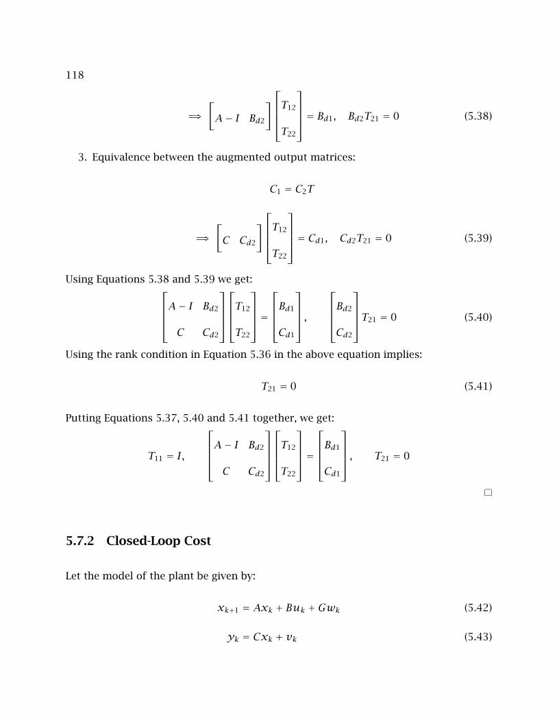
118

=⇒[A− I Bd2

]T12

T22

= Bd1, Bd2T21 = 0 (5.38)

3. Equivalence between the augmented output matrices:

C1 = C2T

=⇒[C Cd2

]T12

T22

= Cd1, Cd2T21 = 0 (5.39)

Using Equations 5.38 and 5.39 we get:A− I Bd2

C Cd2

T12

T22

=Bd1

Cd1

,Bd2

Cd2

T21 = 0 (5.40)

Using the rank condition in Equation 5.36 in the above equation implies:

T21 = 0 (5.41)

Putting Equations 5.37, 5.40 and 5.41 together, we get:

T11 = I,

A− I Bd2

C Cd2

T12

T22

=Bd1

Cd1

, T21 = 0

5.7.2 Closed-Loop Cost

Let the model of the plant be given by:

xk+1 = Axk + Buk +Gwk (5.42)

yk = Cxk + vk (5.43)

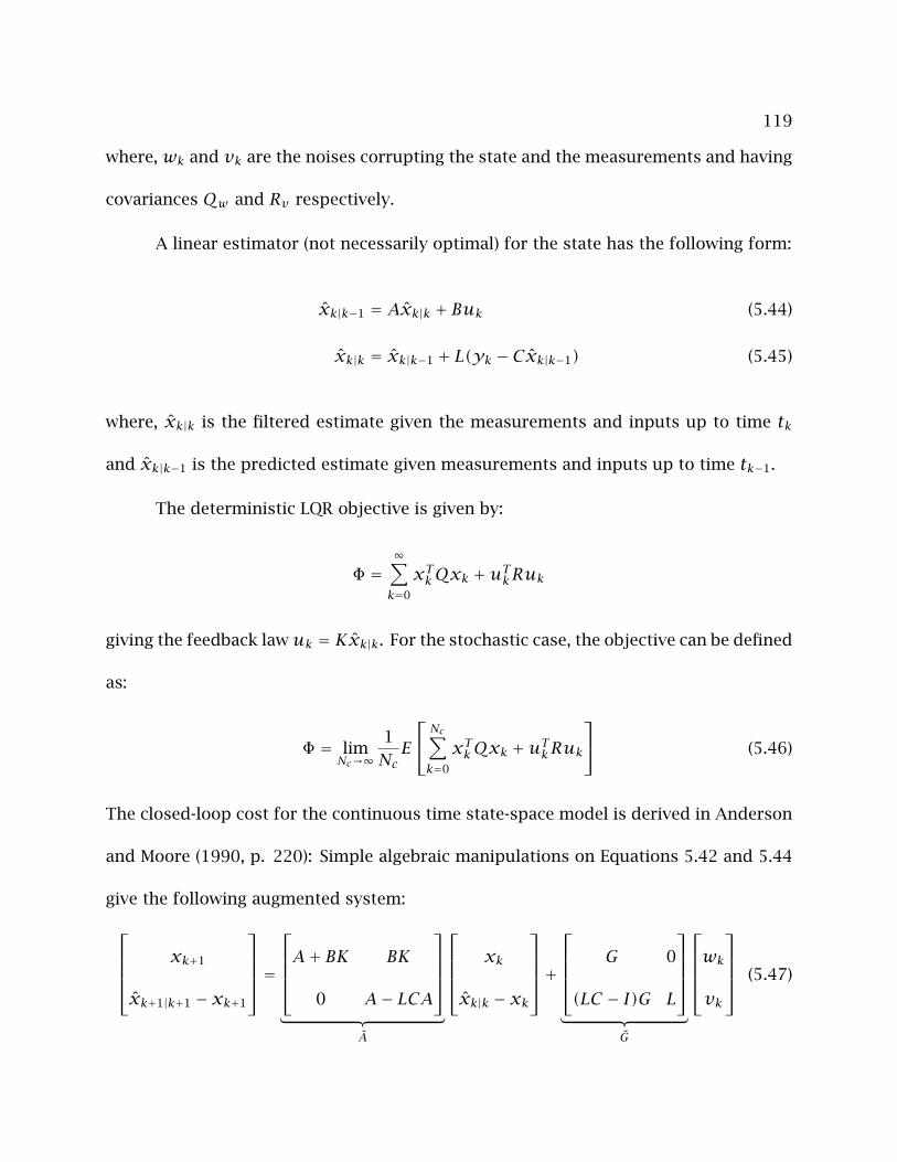
119

where,wk and vk are the noises corrupting the state and the measurements and having

covariances Qw and Rv respectively.

A linear estimator (not necessarily optimal) for the state has the following form:

xk|k−1 = Axk|k + Buk (5.44)

xk|k = xk|k−1 + L(yk − Cxk|k−1) (5.45)

where, xk|k is the filtered estimate given the measurements and inputs up to time tk

and xk|k−1 is the predicted estimate given measurements and inputs up to time tk−1.

The deterministic LQR objective is given by:

Φ =∞∑k=0

xTkQxk +uTkRuk

giving the feedback lawuk = Kxk|k. For the stochastic case, the objective can be defined

as:

Φ = limNc→∞

1NcE

Nc∑k=0

xTkQxk +uTkRuk

(5.46)

The closed-loop cost for the continuous time state-space model is derived in Anderson

and Moore (1990, p. 220): Simple algebraic manipulations on Equations 5.42 and 5.44

give the following augmented system:

xk+1

xk+1|k+1 − xk+1

=A+ BK BK

0 A− LCA

︸︷︷︸

A

xk

xk|k − xk

+ G 0

(LC − I)G L

︸︷︷︸

G

wkvk

(5.47)

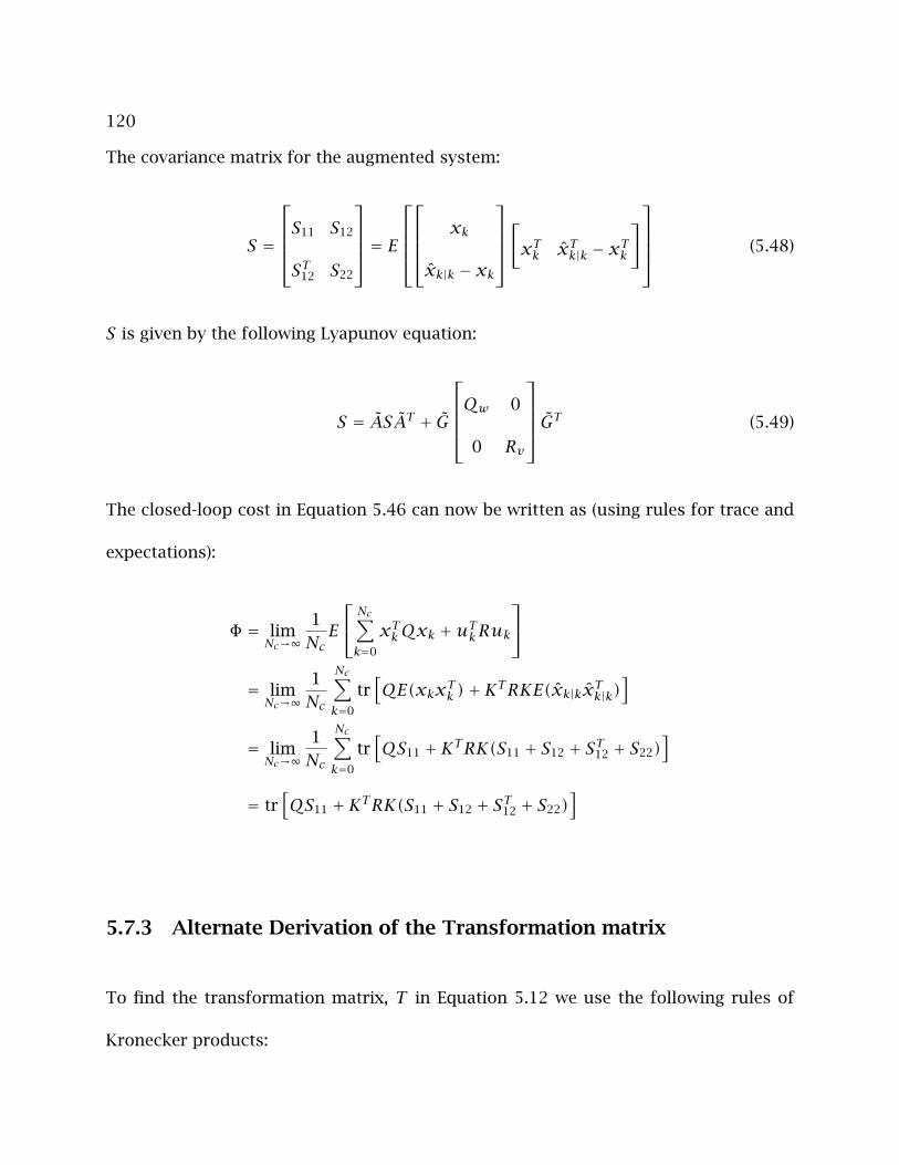
120

The covariance matrix for the augmented system:

S =

S11 S12

ST12 S22

= E xk

xk|k − xk

[xTk xTk|k − xTk

] (5.48)

S is given by the following Lyapunov equation:

S = ASAT + G

Qw 0

0 Rv

GT (5.49)

The closed-loop cost in Equation 5.46 can now be written as (using rules for trace and

expectations):

Φ = limNc→∞

1NcE

Nc∑k=0

xTkQxk +uTkRuk

= limNc→∞

1Nc

Nc∑k=0

tr[QE(xkxTk )+KTRKE(xk|kxTk|k)

]

= limNc→∞

1Nc

Nc∑k=0

tr[QS11 +KTRK(S11 + S12 + ST12 + S22)

]

= tr[QS11 +KTRK(S11 + S12 + ST12 + S22)

]

5.7.3 Alternate Derivation of the Transformation matrix

To find the transformation matrix, T in Equation 5.12 we use the following rules of

Kronecker products:

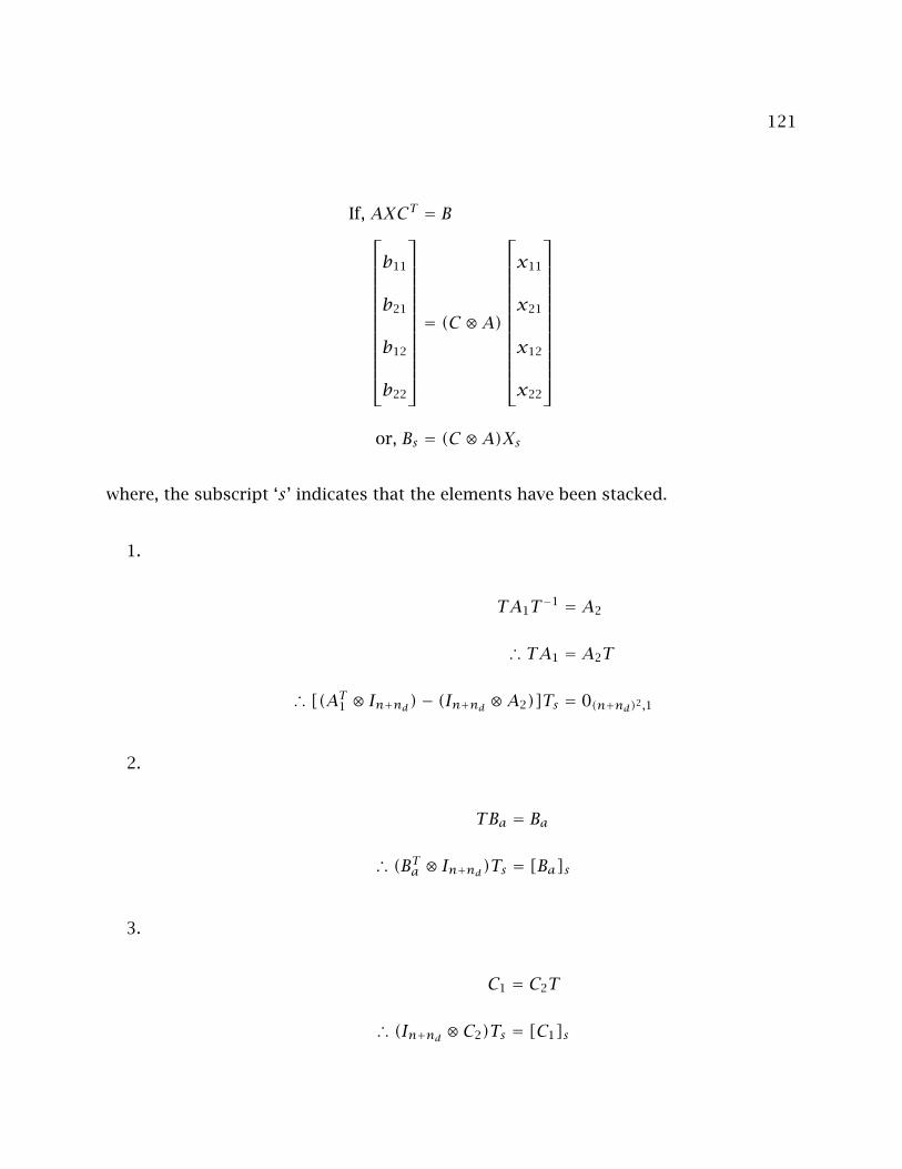
121

If, AXCT = B

b11

b21

b12

b22

= (C ⊗A)

x11

x21

x12

x22

or, Bs = (C ⊗A)Xs

where, the subscript ‘s’ indicates that the elements have been stacked.

1.

TA1T−1 = A2

∴ TA1 = A2T

∴ [(AT1 ⊗ In+nd)− (In+nd ⊗A2)]Ts = 0(n+nd)2,1

2.

TBa = Ba

∴ (BTa ⊗ In+nd)Ts = [Ba]s

3.

C1 = C2T

∴ (In+nd ⊗ C2)Ts = [C1]s

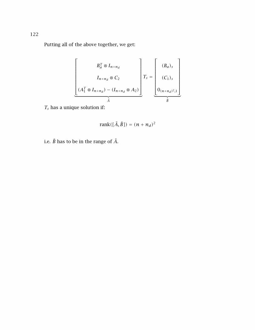
122

Putting all of the above together, we get:

BTa ⊗ In+nd

In+nd ⊗ C2

(AT1 ⊗ In+nd)− (In+nd ⊗A2)

︸︷︷︸

A

Ts =

(Ba)s

(C1)s

0(n+nd)2,1

︸︷︷︸

B

Ts has a unique solution if:

rank([A, B]) = (n+nd)2

i.e. B has to be in the range of A.

123

Chapter 6

Connections between ALS and Maximum

Likelihood Estimation (MLE)

It is well known that a Bayesian estimation procedure gives the minimum variance esti-

mates for the parameters when the errors in the measurements are distributed normally

(Box and Tiao (1973, p. 310);Anderson and Moore (1979, p. 32)). In the ALS technique,

the estimated parameters are the covariances Qw , Rv . However, the errors in the pa-

rameter estimates are not distributed normally. Section 4.1 in Chapter 4 presents more

details about the minimum variance estimation procedure for the ALS technique. In

this chapter, we formulate the maximum likelihood estimation (MLE) procedure for the

covariances Qw , Rv given a set of data y1, · · · , yNd and u1, · · · , uNd for the linear

time-invariant state-space model. We also find the connections between the ALS formu-

lation and the MLE formulation and present an iterative technique to find the maximum

likelihood estimates using the ALS formulation.

124

The Bayesian estimator for the covariances Qw , Rv involves finding the posterior

expectation of the covariances conditional on the given data. In the limit of large data or

an uninformative prior, the a-priori distribution of the covariances becomes negligible

and Bayesian estimation becomes equivalent to the maximum likelihood estimation.

ML estimation procedures aim to maximize the likelihood function with respect to the

parameters.

The literature on solving the MLE problem usually include the state-space matrices

A,B,C as unknowns in addition the covariancesQw , Rv e.g Schweppe (1965). If we start

with the linear time-invariant state-space model and subtract out the state estimates

from the actual state we get the following L-innovations form of the model as shown in

Equations 3.1a and 3.1b in Chapter 3:

εk+1 = (A−ALC)︸︷︷︸A

εk +[G −AL

]︸︷︷︸

G

wkvk

(6.1a)

Yk = Cεk + vk (6.1b)

The unknown noise covariance is:

cov

wkvk

=

Qw 0

0 Rv

We can then write the innovations form of the log likelihood function as shown in

Schweppe (1965):

−2 lnLY (θ) =Nd∑k=1

ln|Σ(θ)| +Nd∑k=1

Yk(θ)TΣ(θ)−1Yk(θ) (6.2)

125

in which LY (θ) is the likelihood function and Σ = CPCT+Rv with P the covariance of εk.

θ is the vector containing the unknowns A,B,C,G,Qw , Rv . If the state-space matrices

A,B,C,G are assumed to be known, then the estimation of the unknown covariances

Qw , Rv follows an iterative scheme:

• Guess Qw , Rv and stack them in a vector θ = [(Qw)s , (Rv)s]

• Calculate Σ = CPCT + Rv and Yk using the guessed values for the covariances

• Compute the innovations form of the likelihood function from Equation 6.2 and

find a gradient direction to maximize LY (θ)

• Iterate until the estimates converge

As emphasized by Shumway and Stoffer (2000, chap. 4), the L-innovations Yk

are dependent on the parameter θ and the likelihood function is a highly nonlinear

and complicated function of θ. Newton-Raphson methods have been suggested in the

literature to recursively update the parameters and to maximize the objective function

in Equation 6.2. A more robust algorithm was given by Shumway and Stoffer (1982)

based on the EM (expectation-maximization) algorithm originally used by Dempster et al.

(1977). The EM algorithm is also an iterative procedure that like other algorithms, fails

to converge to the global optimum starting from a bad initial guess.

In this chapter, we present a simplification of the maximum likelihood estimation

technique using matrix derivatives and the ALS formulation in Chapter 3.

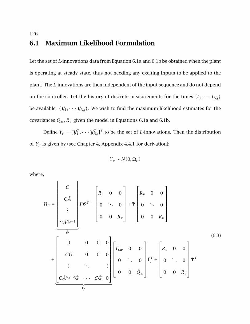
126

6.1 Maximum Likelihood Formulation

Let the set of L-innovations data from Equation 6.1a and 6.1b be obtained when the plant

is operating at steady state, thus not needing any exciting inputs to be applied to the

plant. The L-innovations are then independent of the input sequence and do not depend

on the controller. Let the history of discrete measurements for the times t1, · · · tNd

be available: Y1, · · ·YNd. We wish to find the maximum likelihood estimates for the

covariances Qw , Rv given the model in Equations 6.1a and 6.1b.

Define Yp = [YT1 , · · ·YTNd]T to be the set of L-innovations. Then the distribution

of Yp is given by (see Chapter 4, Appendix 4.4.1 for derivation):

Yp ∼ N(0,Ωp)

where,

Ωp =

C

CA

...

CANd−1

︸︷︷︸

O

POT +

Rv 0 0

0. . . 0

0 0 Rv

+ Ψ

Rv 0 0

0. . . 0

0 0 Rv

+

0 0 0 0

CG 0 0 0

.... . .

...

CANd−2G · · · CG 0

︸︷︷︸

Γf

Qw 0 0

0. . . 0

0 0 Qw

Γ Tf +

Rv 0 0

0. . . 0

0 0 Rv

ΨT

(6.3)

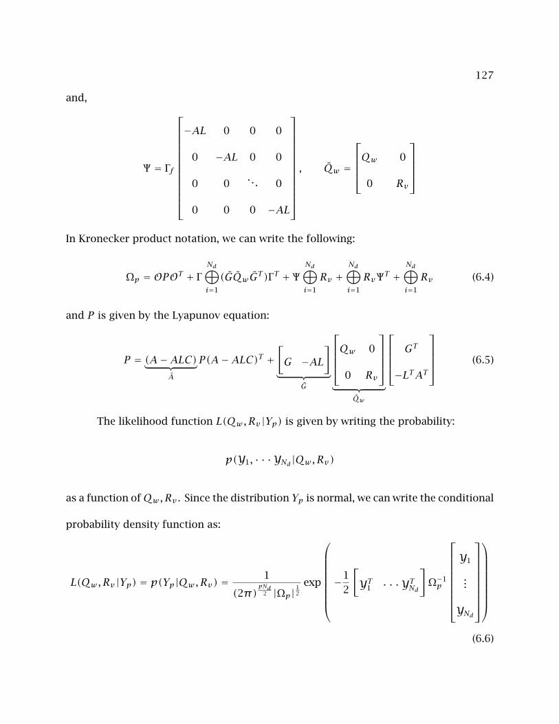
127

and,

Ψ = Γf

−AL 0 0 0

0 −AL 0 0

0 0. . . 0

0 0 0 −AL

, Qw =

Qw 0

0 Rv

In Kronecker product notation, we can write the following:

Ωp = OPOT + ΓNd⊕i=1

(GQwGT )Γ T + ΨNd⊕i=1

Rv +Nd⊕i=1

RvΨT +Nd⊕i=1

Rv (6.4)

and P is given by the Lyapunov equation:

P = (A−ALC)︸︷︷︸A

P(A−ALC)T +[G −AL

]︸︷︷︸

G

Qw 0

0 Rv

︸︷︷︸

Qw

GT

−LTAT

(6.5)

The likelihood function L(Qw , Rv|Yp) is given by writing the probability:

p(Y1, · · ·YNd|Qw , Rv)

as a function ofQw , Rv . Since the distribution Yp is normal, we can write the conditional

probability density function as:

L(Qw , Rv|Yp) = p(Yp|Qw , Rv) =1

(2π)pNd

2 |Ωp|12

exp

−1

2

[YT1 · · ·YTNd

]Ω−1p

Y1

...

YNd

(6.6)

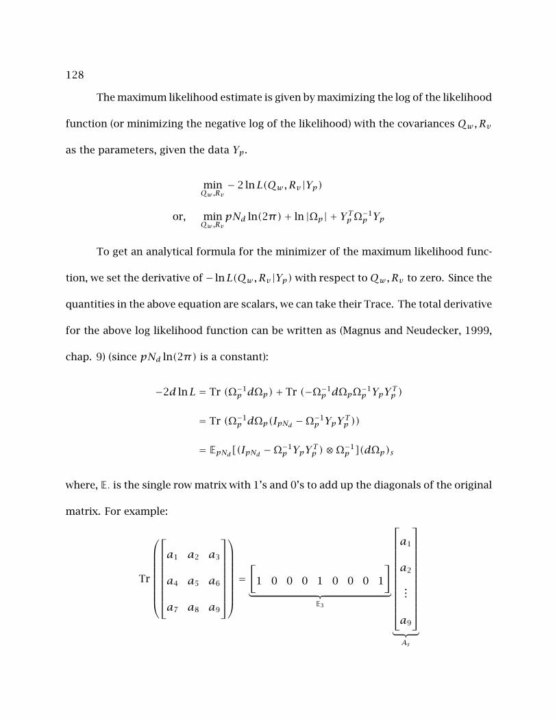
128

The maximum likelihood estimate is given by maximizing the log of the likelihood

function (or minimizing the negative log of the likelihood) with the covariances Qw , Rv

as the parameters, given the data Yp.

minQw ,Rv

− 2 lnL(Qw , Rv|Yp)

or, minQw ,Rv

pNd ln(2π)+ ln |Ωp| + Y TpΩ−1p Yp

To get an analytical formula for the minimizer of the maximum likelihood func-

tion, we set the derivative of − lnL(Qw , Rv|Yp) with respect toQw , Rv to zero. Since the

quantities in the above equation are scalars, we can take their Trace. The total derivative

for the above log likelihood function can be written as (Magnus and Neudecker, 1999,

chap. 9) (since pNd ln(2π) is a constant):

−2d lnL = Tr (Ω−1p dΩp)+ Tr (−Ω−1

p dΩpΩ−1p YpY Tp )

= Tr (Ω−1p dΩp(IpNd −Ω−1

p YpY Tp ))

= EpNd[(IpNd −Ω−1p YpY Tp )⊗Ω−1

p ](dΩp)s

where, E· is the single row matrix with 1’s and 0’s to add up the diagonals of the original

matrix. For example:

Tr

a1 a2 a3

a4 a5 a6

a7 a8 a9

=[

1 0 0 0 1 0 0 0 1

]︸︷︷︸

E3

a1

a2

...

a9

︸︷︷︸As

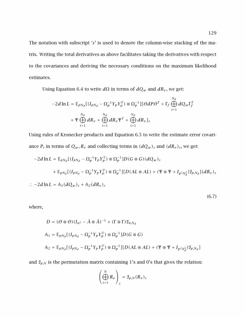
129

The notation with subscript ‘s’ is used to denote the column-wise stacking of the ma-

trix. Writing the total derivatives as above facilitates taking the derivatives with respect

to the covariances and deriving the necessary conditions on the maximum likelihood

estimates.

Using Equation 6.4 to write dΩ in terms of dQw and dRv , we get:

−2d lnL = EpNd[(IpNd −Ω−1p YpY Tp )⊗Ω−1

p ][OdPOT + ΓfNd⊕i=1

dQwΓ Tf

+ ΨNd⊕i=1

dRv +Nd⊕i=1

dRvΨT +Nd⊕i=1

dRv]s

Using rules of Kronecker products and Equation 6.5 to write the estimate error covari-

ance Ps in terms of Qw , Rv and collecting terms in (dQw)s and (dRv)s , we get:

−2d lnL = EpNd[(IpNd −Ω−1p YpY Tp )⊗Ω−1

p ]D(G ⊗G)(dQw)s

+ EpNd[(IpNd −Ω−1p YpY Tp )⊗Ω−1

p ][D(AL⊗AL)+ (Ψ ⊕ Ψ + Ip2N2d)Ip,Nd](dRv)s

∴ −2d lnL = A1(dQw)s +A2(dRv)s

(6.7)

where,

D = (O⊗O)(In2 − A⊗ A)−1 + (Γ ⊗ Γ)In,Nd

A1 = EpNd[(IpNd −Ω−1p YpY Tp )⊗Ω−1

p ]D(G ⊗G)

A2 = EpNd[(IpNd −Ω−1p YpY Tp )⊗Ω−1

p ][D(AL⊗AL)+ (Ψ ⊕ Ψ + Ip2N2d)Ip,Nd]

and Ip,N is the permutation matrix containing 1’s and 0’s that gives the relation: N⊕i=1

Rv

s

= Ip,N(Rv)s

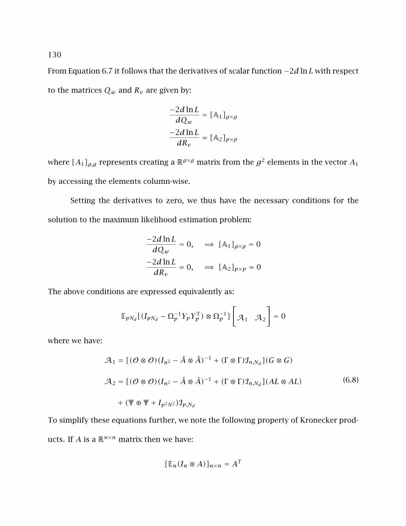
130

From Equation 6.7 it follows that the derivatives of scalar function−2d lnLwith respect

to the matrices Qw and Rv are given by:

−2d lnLdQw

= [A1]g×g

−2d lnLdRv

= [A2]p×p

where [A1]g,g represents creating a Rg×g matrix from the g2 elements in the vector A1

by accessing the elements column-wise.

Setting the derivatives to zero, we thus have the necessary conditions for the

solution to the maximum likelihood estimation problem:

−2d lnLdQw

= 0, =⇒ [A1]g×g = 0

−2d lnLdRv

= 0, =⇒ [A2]p×p = 0

The above conditions are expressed equivalently as:

EpNd[(IpNd −Ω−1p YpY Tp )⊗Ω−1

p ][A1 A2

]= 0

where we have:

A1 = [(O⊗O)(In2 − A⊗ A)−1 + (Γ ⊗ Γ)In,Nd](G ⊗G)

A2 = [(O⊗O)(In2 − A⊗ A)−1 + (Γ ⊗ Γ)In,Nd](AL⊗AL)

+ (Ψ ⊕ Ψ + Ip2N2)Ip,Nd

(6.8)

To simplify these equations further, we note the following property of Kronecker prod-

ucts. If A is a Rn×n matrix then we have:

[En(In ⊗A)]n×n = AT

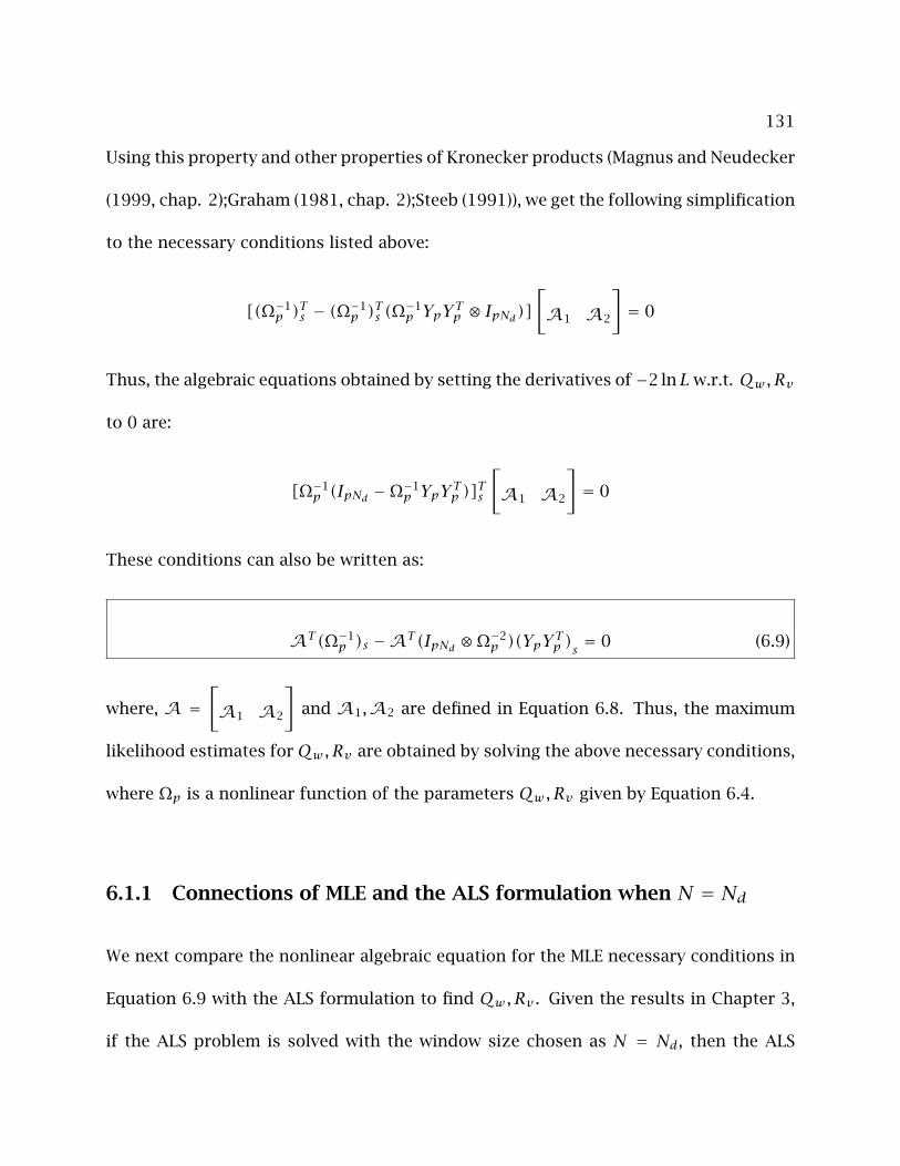
131

Using this property and other properties of Kronecker products (Magnus and Neudecker

(1999, chap. 2);Graham (1981, chap. 2);Steeb (1991)), we get the following simplification

to the necessary conditions listed above:

[(Ω−1p )Ts − (Ω−1

p )Ts (Ω−1p YpY Tp ⊗ IpNd)]

[A1 A2

]= 0

Thus, the algebraic equations obtained by setting the derivatives of−2 lnLw.r.t. Qw , Rv

to 0 are:

[Ω−1p (IpNd −Ω−1

p YpY Tp )]Ts

[A1 A2

]= 0

These conditions can also be written as:

AT (Ω−1p )s −AT (IpNd ⊗Ω−2

p )(YpY Tp )s = 0 (6.9)

where, A =[A1 A2

]and A1,A2 are defined in Equation 6.8. Thus, the maximum

likelihood estimates forQw , Rv are obtained by solving the above necessary conditions,

where Ωp is a nonlinear function of the parameters Qw , Rv given by Equation 6.4.

6.1.1 Connections of MLE and the ALS formulation when N = Nd

We next compare the nonlinear algebraic equation for the MLE necessary conditions in

Equation 6.9 with the ALS formulation to find Qw , Rv . Given the results in Chapter 3,

if the ALS problem is solved with the window size chosen as N = Nd, then the ALS

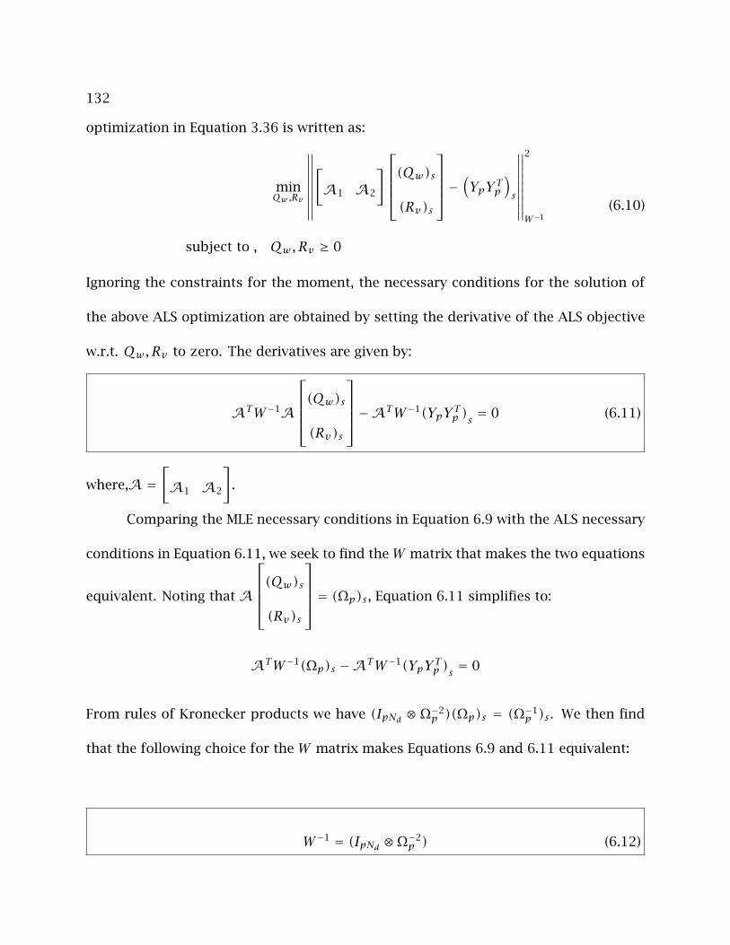
132

optimization in Equation 3.36 is written as:

minQw ,Rv

∥∥∥∥∥∥∥∥∥[A1 A2

](Qw)s(Rv)s

− (YpY Tp )s∥∥∥∥∥∥∥∥∥

2

W−1

subject to , Qw , Rv ≥ 0

(6.10)

Ignoring the constraints for the moment, the necessary conditions for the solution of

the above ALS optimization are obtained by setting the derivative of the ALS objective

w.r.t. Qw , Rv to zero. The derivatives are given by:

ATW−1A

(Qw)s(Rv)s

−ATW−1(YpY Tp )s = 0 (6.11)

where,A=[A1 A2

].

Comparing the MLE necessary conditions in Equation 6.9 with the ALS necessary

conditions in Equation 6.11, we seek to find theW matrix that makes the two equations

equivalent. Noting thatA

(Qw)s(Rv)s

= (Ωp)s , Equation 6.11 simplifies to:

ATW−1(Ωp)s −ATW−1(YpY Tp )s = 0

From rules of Kronecker products we have (IpNd ⊗ Ω−2p )(Ωp)s = (Ω−1

p )s . We then find

that the following choice for the W matrix makes Equations 6.9 and 6.11 equivalent:

W−1 = (IpNd ⊗Ω−2p ) (6.12)

133

Thus, to solve the MLE problem as a least-squares problem, we need to set N = Nd

and the least-squares weight as given in Equation 6.12. However, note that the weight

W is still a complicated nonlinear function of the unknown covariances Qw , Rv and an

iterative procedure is required to solve Equation 6.11.

An iterative procedure to calculate the maximum likelihood estimates using least-

squares is:

1. Guess a value for the covariances: Qw , Rv and calculate Ωp from Equation 6.4

2. Calculate the ML weighting W−1 using Equation 6.12

3. Use the weighted ALS formulation with the weight W−1 to estimate new set of

covariances Qw , Rv using the optimization in Equation 6.10

4. Repeat the above steps till convergence

6.1.2 MLE and ALS with Window Size N

In the previous section the comparison between the ALS and the MLE formulations

was obtained by choosing the ALS window size as N = Nd. When N is chosen to be

smaller than the data length Nd, similarities can still be seen between the ALS and MLE

formulations.

As in the previous section, we set the derivative of the ALS objective with a window

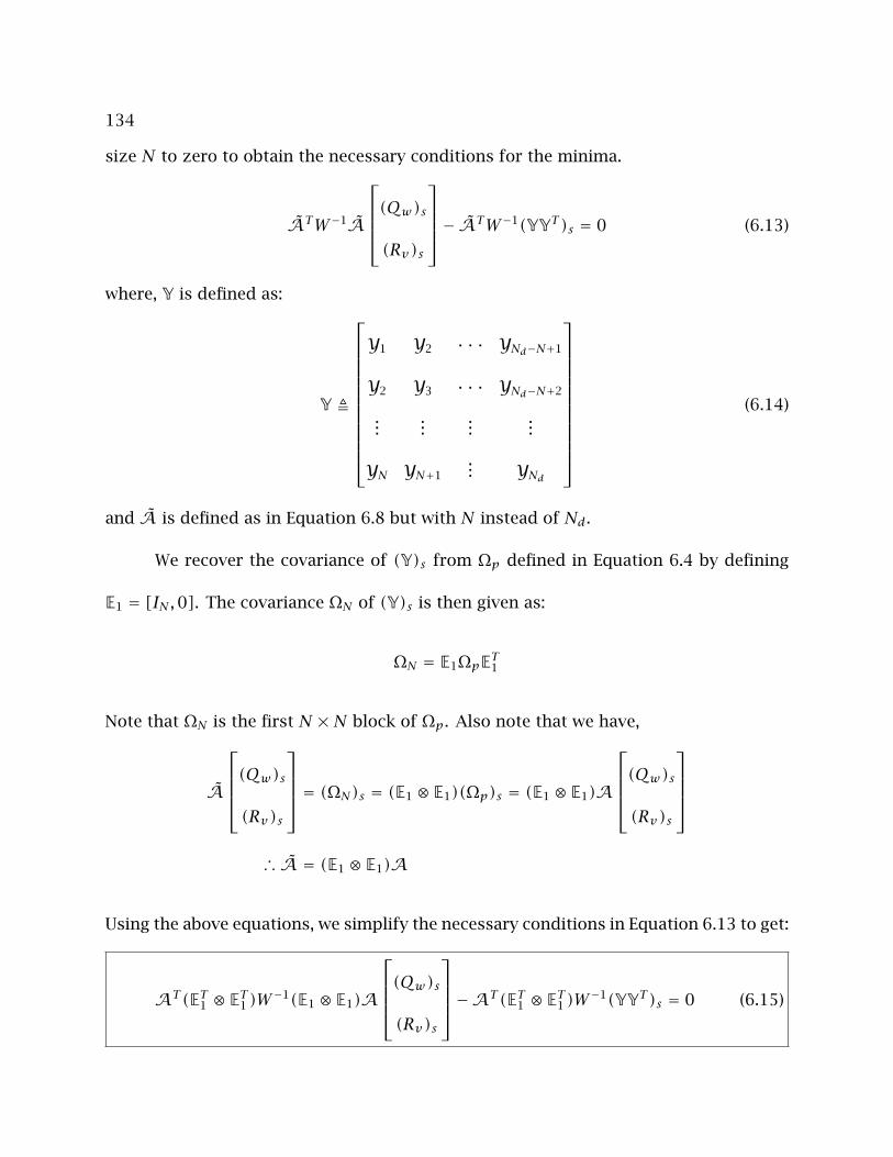
134

size N to zero to obtain the necessary conditions for the minima.

ATW−1A

(Qw)s(Rv)s

− ATW−1(YYT )s = 0 (6.13)

where, Y is defined as:

Y Õ

Y1 Y2 · · · YNd−N+1

Y2 Y3 · · · YNd−N+2

......

......

YN YN+1... YNd

(6.14)

and A is defined as in Equation 6.8 but with N instead of Nd.

We recover the covariance of (Y)s from Ωp defined in Equation 6.4 by defining

E1 = [IN ,0]. The covariance ΩN of (Y)s is then given as:

ΩN = E1ΩpET1

Note that ΩN is the first N ×N block of Ωp. Also note that we have,

A

(Qw)s(Rv)s

= (ΩN)s = (E1 ⊗ E1)(Ωp)s = (E1 ⊗ E1)A

(Qw)s(Rv)s

∴ A = (E1 ⊗ E1)A

Using the above equations, we simplify the necessary conditions in Equation 6.13 to get:

AT (ET1 ⊗ ET1 )W−1(E1 ⊗ E1)A

(Qw)s(Rv)s

−AT (ET1 ⊗ ET1 )W−1(YYT )s = 0 (6.15)

135

Using an analysis similar to the previous section, to get the MLE necessary conditions

in Equation 6.9 to be equivalent to the conditions in Equation 6.15 we need W defined

to satisfy the following condition:

(ET1 ⊗ ET1 )W−1(E1 ⊗ E1) = (IpNd ⊗Ω−2p )

The weighted ALS conditions in Equation 6.15 then becomes:

AT (Ω−1p )s −AT (IpNd ⊗Ω−2

p )M(YYT )s = 0

Comparing the above Equation with the MLE estimation Equation 6.9 we see that M is

some permutation matrix containing 1’s and 0 such that it satisfies:

M(YYT )s = (YpY Tp )s (6.16)

Notice that YpY Tp contains autocovariances for lags up to Nd while YYT contains auto-

covariances for lags only up to the window size N. Thus, from the above equation it

is clear that there exists no permutation matrix M that satisfies Equation 6.16. Thus

the parameter N cannot be introduced to give an equivalent ALS weight when doing

maximum likelihood estimation.

6.2 Conclusions

The application of the maximum likelihood estimation procedure was not tested on

actual data sets due to large memory requirements even for problems of small dimen-

sions. We however, expect the performance of the ML formulation to be similar to the

136

weighted least-squares formulation of the ALS problem given in Section 4.1. Solving

the ALS problem with N = Nd and iterating till convergence is a practical method of

implementation of the maximum likelihood formulation provided the computation is

feasible.

137

Chapter 7

Industrial Applications of the ALS

Technique and Extension to Nonlinear

Models 1

Most physical systems have nonlinear dynamics when modelled from first principles.

Even a simple reaction such as A + B → C has a nonlinear rate of reaction r = kCACB

and the rate constant k has a nonlinear dependence on the temperature. A linear

time-invariant approximation to the nonlinear model is often not valid when the dy-

namics are significantly nonlinear or the plant is operated under batch mode eg. a

co-polymerization reactor requiring batch transitions. Techniques that have been de-

veloped for linear time-invariant models then have to be extended to nonlinear models

and their validity tested.

1Portions of this chapter are to appear in Rajamani et al. (October, 2007)

138

In this chapter, we present the nonlinear extension to the Autocovariance Least-

Squares (ALS) technique developed in Chapters 3 and 5. A time-varying ALS formulation

is applied to real industrial data from a nonlinear blending drum used at ExxonMobil

Chemical Company 2. Section 7.2 presents the model and the results to illustrate the

value of the nonlinear extension to the ALS technique. Section 7.3 shows the equivalence

between a current industrial state estimator implementation called the Implicit Dynamic

Feedback (IDF) and integrating input disturbance models. The results from Chapter 5

are used in Section 7.6 to identify appropriate covariances for the disturbance structure

in Shell’s SMOC implementation.

7.1 Noise Covariance Estimation for Nonlinear Models

Consider the following nonlinear state-space model:

xk+1 = f(xk, uk)+ g(xk, uk)wk

yk = h(xk)+ vk(7.1)

where, x ∈ Rn is the state, y ∈ Rp are the measurements, uk ∈ Rm are the inputswk, vk

and the noises corrupting the state and the measurements respectively. The noises

wk, vk are assumed to be from a Gaussian distribution with mean zero and covariances

Qw , Rv . Also, wk, vk are assumed to be uncorrelated with each other.

Let the state estimates be obtained starting from an arbitrary initial value using

a time-varying stable filter gain sequence Lk. An example of such a filter gain would

2ExxonMobil Chemical Company is a division of ExxonMobil Corporation

139

be the sequence obtained by implementing the extended Kalman filter (EKF). The only

condition on the time-varying gains Lk is that they are stable (see Assumption 7.1). The

state estimation can then be described by the following equations:

xk+1|k = f(xk|k, uk)

xk|k = xk|k−1 − Lk(yk − yk|k−1)

yk|k−1 = h(xk|k−1)

(7.2)

Here, xk|k−1 represents the predicted estimate of the state xk given measurements and

inputs up to time tk−1 and xk|k the filtered estimate given measurements and inputs up

to time tk. Subtracting the predicted state estimates in Equation 7.2 from the plant in

Equation 7.1, we get an approximate time-varying linear model for the innovations:

εk+1 ≈ (Ak −AkLkCk)︸︷︷︸Ak

εk +[Gk −AkLk

]︸︷︷︸

Gk

wkvk

︸︷︷︸wk

Yk ≈ Ckεk + vk

(7.3)

where, εk = (xk − xk|k−1) denotes the state estimate error and Yk the innovations.

The noises wk, vk driving the innovations sequence are assumed to drawn from time-

invariant covariances Qw , Rv .

The time-varying approximation of the nonlinear model is defined by the follow-

ing linearization:

Ak =∂f(xk, uk)∂xTk

∣∣∣∣∣(xk|k−1,uk)

, Gk = g(xk|k−1, uk), Ck =∂h(xk)∂xTk

∣∣∣∣∣xk|k−1

(7.4)

140

A second possibility for the linear approximation is to evaluate the terms in Equation

7.4 at xk|k instead of xk|k−1 (Anderson and Moore, 1979). The next section presents

a technique for estimating the covariances Qw , Rv using autocovariances of data at

different time lags.

7.1.1 Time-varying Autocovariance Least-Squares Technique

The Autocovariance Least-Squares (ALS) covariance estimation technique described in

Chapter 3 was developed for linear time-invariant models. When using nonlinear or

time-varying models, a key difference is that the estimate error covariance Pk = E[(xk−

xk|k−1)(xk − xk|k−1)] is the time-varying solution to the Riccati equation and does not

reach a steady state value. No simple equation can then be written for Pk in terms

of Qw , Rv and the system matrices as in the linear time-invariant case. The following

Assumption 7.1 however, allows extension of the ALS technique to time-varying and

nonlinear systems.

Assumption 7.1. The time-varying filter gain sequence Lk used in Equation 7.2 are such

that when used in the approximate linearization given by Equation 7.3 they produce a

sequence of Ak = (Ak − AkLkCk) matrices such that the product (∏jk=0 Ai) ≈ 0 as j

increases.

Starting from an arbitrary initial condition ε0 at t0, consider the evolution of

141

Equation 7.3 up to time tk to obtain the following:

Yk = Ck(k−1∏i=0

Ai)ε0 + Ck(k−1∏i=1

AiG0w0 +k−1∏i=2

AiG1w1 + · · · + Gk−1wk−1)+ vk

Yk+j = Ck+j(k+j−1∏i=0

Ai)ε0 + Ck+j(k+j−1∏i=1

AiG0w0 +k+j−1∏i=2

AiG1w1 + · · · + Gk+j−1wk+j−1)+ vk+j

(7.5)

The covariance of wk =

wkvk

is given by Qw =

Qw 0

0 Rv

.

From Assumption 7.1, the index k > 0 is chosen to be large enough such that

∏k−1i=0 Ai ≈ 0. The effect of the initial estimate error ε0 is then negligible in Yk+j for

j > 0. The terms involving ε0 in Equation 7.5 can then be neglected. From Equation 7.5

we get the following expressions for the expectation of the autocovariances at different

lags:

E[YkYTk ] = Ck(k−1∏i=1

AiG0 + · · · + Gk−1)Qw(GT0k−1∏i=1

ATi + · · · + GTk−1)CTk + Rv

E[Yk+jYTk ] = Ck+j(k+j−1∏i=1

AiG0 + · · · +k+j−1∏i=k

AiGk−1)Qw(GT0k−1∏i=1

ATi + · · · + GTk−1)CTk

− Ck+j(k+j−1∏i=k+1

Ai)AkLkRv

(7.6)

In the above Equation 7.6, we define∏ji=k Ai = I for all j ≤ k.

Remark 7.1. In general, instead of starting from the initial condition ε0 at t0, we can start

from an initial condition εm at tm and calculate the expectations as above, provided the

142

indices k and m are such that the following condition holds as in Assumption 7.1:

m+k−1∏i=m

Ai ≈ 0

Let the autocovariance matrix Rk(N) be defined as the expectation of the inno-

vations data at different time lags over a user defined window N (Jenkins and Watts,

1968).

Rk(N) = E

YkYTk

...

Yk+N−1YTk

(7.7)

Using Equations 7.5 and 7.7, we get:

Rk(N) =

I

−Ck+1AkLk

...

−Ck+N−1(∏k+N−2i=k+1 Ai)AkLk

︸︷︷︸

Ψ1

Rv + ΓΩ1

k⊕i=1

QwΩT1 ΓT1 + ΓΩ2

k⊕i=1

RvΩT2 ΓT1 (7.8)

where the matrices are defined as follows and dimensioned appropriately:

Γ =

Ck(

∏k−1i=1 Ai) · · · Ck

.... . .

...

Ck+N−1(∏k+N−2i=1 Ai) · · · Ck+N−1(

∏k+N−2i=k Ai)

(7.9)

and

Ω1 =

G0 . . . 0

.... . .

...

0 . . . Gk−1

, Ω2 =

−A0L0 . . . 0

.... . .

...

0 . . . −Ak−1Lk−1

, Γ T1 =

(∏k−1i=1 A

Ti )C

Tk

...

CTk

(7.10)

143

Γ1 is the first row block of the Γ matrix. In the above equation and in the remainder

of this chapter we use standard properties and symbols of Kronecker products (Steeb

(1991) and Graham (1981, chap. 2)). ⊗ is the standard symbol for the Kronecker product

and⊕

is the symbol for the Kronecker sum, satisfying the following property:

k⊕i=1

Qw = (Ik ⊗Qw)

We use the subscript ‘s’ to denote the column-wise stacking of the elements of a

matrix into a vector. Stacking both sides of Equation 7.8 we then get:

[Rk(N)]s = (Γ1Ω1 ⊗ ΓΩ1)Ig,k(Qw)s +[(Γ1Ω2 ⊗ ΓΩ2)Ip,k + Ip ⊗ Ψ

](Rv)s (7.11)

Here, Ip,N is a permutation matrix containing 1’s and 0’s and satisfying the relation:

N⊕i=1

Rv

s

= Ip,N(Rv)s

If we have an estimate of the autocovariance matrixRk(N) denoted by Rk(N) and

let bk = [Rk(N)]s , then from Equation 7.11 we can formulate a positive semidefinite

constrained least-squares problem in the unknown covariances Qw , Rv (Chapter 3 and

Odelson et al. (2006b)). The optimization to be solved is given by:

Φk = minQw ,Rv

∥∥∥∥∥∥∥∥∥Ak

(Qw)s(Rv)s

− bk∥∥∥∥∥∥∥∥∥

2

W

subject to, Qw , Rv ≥ 0, Qw = QTw , Rv = RTv

(7.12)

144

where,

Ak =[Ak1 Ak2

]

Ak1 = (Γ1Ω1 ⊗ ΓΩ1)Ig,k

Ak2 =[(Γ1Ω2 ⊗ ΓΩ2)Ip,k + Ip ⊗ Ψ

](7.13)

We will refer to the optimization in Equation 7.12 as the Autocovariance Least-Squares

(ALS) technique. Necessary and sufficient conditions for the uniqueness of the ALS

optimization in Equation 7.12 are given in Chapter 3. For the estimates of Qw , Rv in

the ALS optimization to have minimum variance the weighting matrix W in the ALS

objective is given by W = T−1k where Tk is the covariance of bk (Aitken, 1935).

The matrices Ak and the vector bk in the Equation 7.12 have the time subscript

‘k’ to emphasize that these quantities are time-varying and based on the time-varying

approximation given in Equation 7.3.

Since the only data set available for estimating the time-varying quantity Rk(N)

defined in Equation 7.7 is Yk, · · · ,Yk+N−1, the only calculable estimate of bk is given

by:

bk = [Rk(N)]s =

YkYTk

...

Yk+N−1YTk

s

(7.14)

At every time instant tk, we compute the quantitiesAk and bk from Equations 7.13

and 7.14. To simplify the computation, the matrices Γ ,Ω1,Ω2, Γ1 defined in Equations

7.9 and 7.10 and used in the calculation of Ak, can be computed starting from an

145

initial condition at time tm rather than t0 as given in Remark 7.1. We then use a sliding

window strategy to compute the time-varying matricesAk and bk. Figure 7.1 illustrates

the calculation procedure.

k

YkYk, · · · ,Yk+N−1 ⇒ Ak, bk

Yk+1, · · · ,Yk+N ⇒ Ak+1, bk+1

Yk+6, · · · ,Yk+N+5 ⇒ Ak+6, bk+6

t0

Sliding Window

Figure 7.1: Strategy for calculating the time-varyingAk matrices in Equation 7.13

Using the computed time-varying matrices and the ALS formulation in Equation

7.12, we can then solve the following optimization for a set of data of length Nd to

estimate Qw , Rv :

Φ = minQw ,Rv

∥∥∥∥∥∥∥∥∥∥∥∥∥∥

Ak

...

ANd−N+1

(Qw)s(Rv)s

−

bk

...

bNd−N+1

∥∥∥∥∥∥∥∥∥∥∥∥∥∥

2

Wf

subject to, Qw , Rv ≥ 0, Qw = QTw , Rv = RTv

(7.15)

Since bk, bk+1, · · · are not independent, the weighting matrix Wf is not block diagonal.

The formula for Wf is a complicated function of the unknown covariances Qw , Rv and

146

an iterative procedure is required for its calculation (see Section 4.1, Chapter 4). We use

Wf = I to avoid the expensive and nonlinear calculation.

Remark 7.2. Notice that if the system is time-invariant we have Ak = · · · = ANd−N+1

and we can then recover the time-invariant ALS optimization presented in Section 3.2 in

Chapter 3.

Remark 7.3. Assumption 7.1 is a simple practical requirement that the time-varying

linear approximation of the full nonlinear model has a gain sequence that makes the

estimate error asymptotically zero. This requirement is satisfied in most industrial appli-

cations that use a linear approximation to design the state estimator.

7.2 Industrial Blending Drum Example

Figure 7.2 shows a schematic diagram of a blending drum where two components,

monomer A and co-monomer B are mixed with a diluent to give the correct propor-

tions for the blends used as the feed for the different grades of polymers made in the

reactors. The diagram is a representation of a blending process unit at ExxonMobil

Chemical Company. The mass fractions of A and B inside the blending drum are rep-

resented by XA and XB . The blending tank is elliptical at the bottom and the dynamics

of the blending process are nonlinear.

The states of the system are the mass fractionsXA, XB and the level in the drum h.

The nonlinearity in the drum is given by the following equations where V is the volume

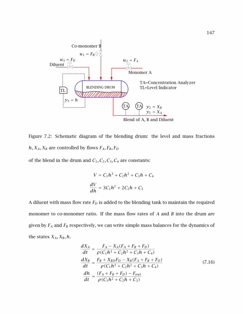
147

BLENDING DRUM

Blend of A, B and Diluent

TA TA

TL

Diluent

TA=Concentration AnalyzerTL=Level Indicator

Monomer A

Co-monomer B

y3 = h

u2 = FAu3 = FDu1 = FB

y2 = XBy1 = XA

Figure 7.2: Schematic diagram of the blending drum: the level and mass fractions

h,XA, XB are controlled by flows FA, FB, FD

of the blend in the drum and C1, C2, C3, C4 are constants:

V = C1h3 + C2h2 + C3h+ C4

dVdh= 3C1h2 + 2C2h+ C3

A diluent with mass flow rate FD is added to the blending tank to maintain the required

monomer to co-monomer ratio. If the mass flow rates of A and B into the drum are

given by FA and FB respectively, we can write simple mass balances for the dynamics of

the states XA, XB, h.

dXAdt

= FA −XA(FA + FB + FD)ρ(C1h3 + C2h2 + C3h+ C4)

dXBdt

= FB +XBDFD −XB(FA + FB + FD)ρ(C1h3 + C2h2 + C3h+ C4)

dhdt= (FA + FB + FD)− Foutρ(C1h2 + C2h+ C3)

(7.16)

148

where, XBD is the mass fraction of B in the diluent feed, Fout is the measured out flow

rate of the blend and ρ is the recorded density of the blend.

The controlled variables are the level of inventory in the drum h, the ratio of the

mass fractions of A to B, XAXB in the outlet stream and the fraction XA of A leaving the

drum. Measurements are made for the states XA, XB, h at intervals of one minute.

Five sets of industrial operating data were provided by ExxonMobil Chemical Com-

pany with the characteristics described below:

• Data Set I: Steady state operating data

• Data Set II: Set point change in the liquid level h

• Data Set III: Step change in the in flow rate FB

• Data Set IV: Set point change in the liquid level and the ratio of the monomer to

co-monomer mass fractions

• Data Set V: Same as Data Set IV

The state-space model in discrete time for the above equations can then be rep-

resented as:

xk+1 = f(xk, uk)+Gwk

yk = xk + vk(7.17)

149

in which,

xk =

XA

XB

h

, uk =

FA

FB

FD

The G matrix is chosen as the constant G =[

0 0 1

]Tin the model, which implies the

state noise in h is more significant than the noise in the states XA, XB . The state xk+1 is

calculated by integrating the nonlinear model given in Equation 7.16 from xk over the

discretization time of one minute while keeping the input uk constant. The states and

the measurements are corrupted by noises wk, vk with unknown covariances Qw , Rv

respectively.

7.2.1 Simulation Results

To illustrate the value of the ALS technique applied to a nonlinear model, the data were

generated by drawing noiseswk and vk from known covariancesQw , Rv and simulating

the nonlinear model from Equations 7.16 as given in Equation 7.17. Since a steady state

simulation is equivalent to using a linear time-invariant approximation to the nonlinear

model, the data are simulated by making multiple set point changes to the level in

the drum and implementing a simple PI controller to maintain the level. The set point

changes introduced are such that a simple linear time-invariant approximation of the

full nonlinear model is not valid.

Figure 7.3 shows a plot of the eigenvalues of the time-varying (Ak − AkLkCk)

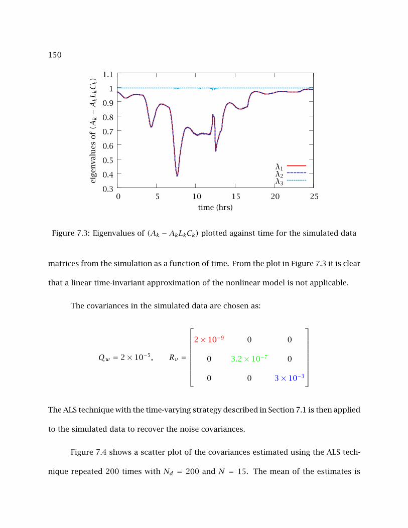
150

0.3

0.4

0.5

0.6

0.7

0.8

0.9

1

1.1

0 5 10 15 20 25

eige

nva

lues

of(A

k−AkL kCk)

time (hrs)

λ1λ2λ3

Figure 7.3: Eigenvalues of (Ak −AkLkCk) plotted against time for the simulated data

matrices from the simulation as a function of time. From the plot in Figure 7.3 it is clear

that a linear time-invariant approximation of the nonlinear model is not applicable.

The covariances in the simulated data are chosen as:

Qw = 2× 10−5, Rv =

2× 10−9 0 0

0 3.2× 10−7 0

0 0 3× 10−3

The ALS technique with the time-varying strategy described in Section 7.1 is then applied

to the simulated data to recover the noise covariances.

Figure 7.4 shows a scatter plot of the covariances estimated using the ALS tech-

nique repeated 200 times with Nd = 200 and N = 15. The mean of the estimates is

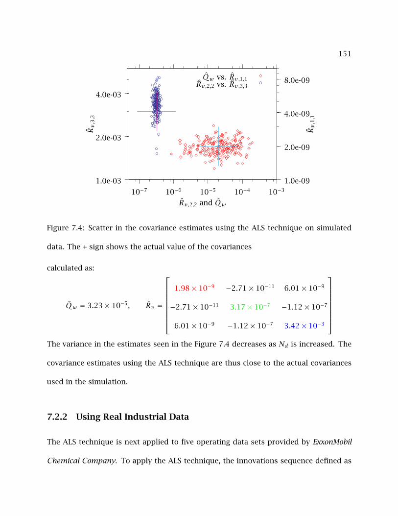
151

1.0e-03

2.0e-03

4.0e-03

10−7 10−6 10−5 10−4 10−3

1.0e-09

2.0e-09

4.0e-09

8.0e-09Rv,3,3

Rv,1,1

Rv,2,2 and Qw

Qw vs. Rv,1,1Rv,2,2 vs. Rv,3,3

Figure 7.4: Scatter in the covariance estimates using the ALS technique on simulated

data. The + sign shows the actual value of the covariances

calculated as:

Qw = 3.23× 10−5, Rv =

1.98× 10−9 −2.71× 10−11 6.01× 10−9

−2.71× 10−11 3.17× 10−7 −1.12× 10−7

6.01× 10−9 −1.12× 10−7 3.42× 10−3

The variance in the estimates seen in the Figure 7.4 decreases as Nd is increased. The

covariance estimates using the ALS technique are thus close to the actual covariances

used in the simulation.

7.2.2 Using Real Industrial Data

The ALS technique is next applied to five operating data sets provided by ExxonMobil

Chemical Company. To apply the ALS technique, the innovations sequence defined as

152

the difference between the measured outputs and the simulated model outputs should

be zero mean. To remove the modelling errors and to ensure zero mean in the inno-

vations, integrating disturbances are added to the inputs and the outputs in the model

(Tenny et al., 2004; Pannocchia and Rawlings, 2002). A state estimator is then used to es-

timate the integrating disturbance vector, which then compensates for the plant/model

mismatch. To ensure detectability of the integrating disturbance model the number of

disturbances is chosen as nd = 3 (Muske and Badgwell, 2002; Pannocchia and Rawlings,

2002) (Also see Remark 7.4).

Remark 7.4. Note that the level in the tank is an integrator and the model of the plant

is not perfect. Hence, when the inputs provided in the data sets is used in the model

simulation, the simulated yk,3 and the measured h from the data can never match. This

issue is resolved by adding an integrating input disturbance to the state h. Also note

that since the dynamics for h are integrating in the open-loop, an output disturbance

model cannot be used to remove this mismatch (Qin and Badgwell, 2003; Dougherty and

Cooper, 2003).

The model in Equation 7.17 augmented with the disturbance model is given by:

xk+1 = f(xk, uk)+ Bddk +Gwk (7.18)

dk+1 = dk + ξk (7.19)

yk = xk + Cddk + vk (7.20)

where, dk is the integrating disturbance and ξ ∼ N(0,Qξ) is the noise model for the

153

disturbance. We make the following choice for Bd and Cd:

Bd =

0 0 0

0 0 0

0 0 1

, Cd =

1 0 0

0 1 0

0 0 0

The model is simulated with the inputs and measurements given in the data sets and

the extended Kalman filter (EKF) used as the initial state estimator. Since the covari-

ances affecting the operating data are unknown, the following initial guesses for the

covariances are used to calculate the initial estimator gain sequence in the EKF:

Qw = 1× 10−14, Qξ = 10−9 × I3, Rv = 2× diag (10−7,10−5,10−3) (7.21)

These choices are made by assigning the variance in the operating data measurements

to the corresponding diagonal elements of Rv and choosing small values for Qw ,Qξ .

This choice follows the rough industrial guidelines of assigning the noise covariances

to the output when calculating state estimator gains.

The initial estimator gain sequence Lk obtained by implementing the EKF satis-

fies Assumption 7.1 and hence the ALS technique can be applied to the operating data.

With the above model and the industrial data, the covariances Qw ,Qξ and Rv are esti-

mated. The diagonal elements of the estimated covariances Qw ,Qξ, Rv using the ALS

technique for the five data sets are shown in Figures 7.5 and 7.6. The figures show that

the estimated covariances have consistent values across all the five industrial data sets

provided. These estimated covariances are then used to calculate new filter gains for

the EKF. A snapshot of the measurements compared against the model estimates with

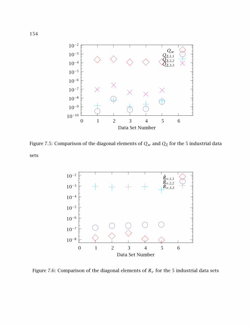
154

10−10

10−9

10−8

10−7

10−6

10−5

10−4

10−3

10−2

0 1 2 3 4 5 6

Data Set Number

QwQξ,1,1Qξ,2,2Qξ,3,3

Figure 7.5: Comparison of the diagonal elements ofQw andQξ for the 5 industrial data

sets

10−8

10−7

10−6

10−5

10−4

10−3

10−2

0 1 2 3 4 5 6

Data Set Number

Rv,1,1Rv,2,2Rv,3,3

Figure 7.6: Comparison of the diagonal elements of Rv for the 5 industrial data sets

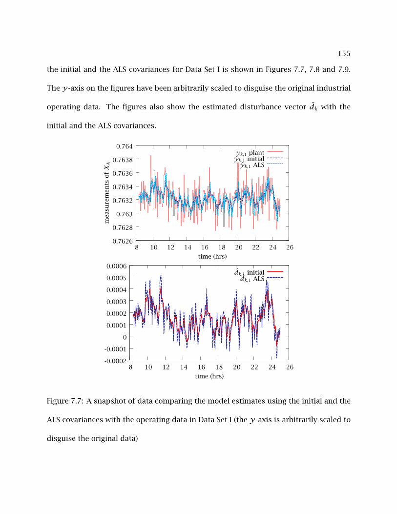
155

the initial and the ALS covariances for Data Set I is shown in Figures 7.7, 7.8 and 7.9.

The y-axis on the figures have been arbitrarily scaled to disguise the original industrial

operating data. The figures also show the estimated disturbance vector dk with the

initial and the ALS covariances.

0.7626

0.7628

0.763

0.7632

0.7634

0.7636

0.7638

0.764

8 10 12 14 16 18 20 22 24 26

mea

sure

men

tso

fXA

time (hrs)

yk,1 plantyk,1 initialyk,1 ALS

-0.0002

-0.0001

0

0.0001

0.0002

0.0003

0.0004

0.0005

0.0006

8 10 12 14 16 18 20 22 24 26

time (hrs)

dk,1 initialdk,1 ALS

Figure 7.7: A snapshot of data comparing the model estimates using the initial and the

ALS covariances with the operating data in Data Set I (the y-axis is arbitrarily scaled to

disguise the original data)

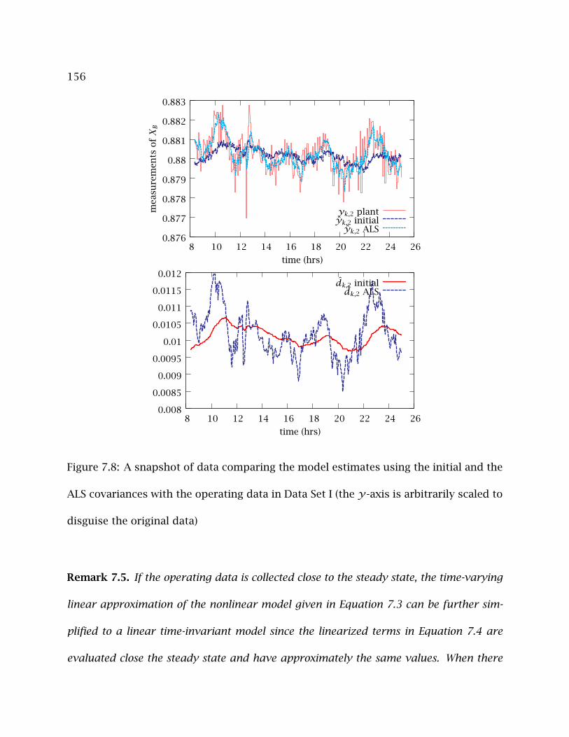
156

0.876

0.877

0.878

0.879

0.88

0.881

0.882

0.883

8 10 12 14 16 18 20 22 24 26

mea

sure

men

tso

fXB

time (hrs)


0.008

0.0085

0.009

0.0095

0.01

0.0105

0.011

0.0115

0.012

8 10 12 14 16 18 20 22 24 26

time (hrs)





Remark 7.5. If the operating data is collected close to the steady state, the time-varying

linear approximation of the nonlinear model given in Equation 7.3 can be further sim-

plified to a linear time-invariant model since the linearized terms in Equation 7.4 are

evaluated close the steady state and have approximately the same values. When there

157

58.8

59

59.2

59.4

59.6

59.8

60

60.2

60.4

60.6

60.8

8 10 12 14 16 18 20 22 24 26

mea

sure

men

tso

fh

time (hrs)


-0.05

-0.045

-0.04

-0.035

-0.03

-0.025

-0.02

8 10 12 14 16 18 20 22 24 26

time (hrs)





are multiple set point changes in the operating data, the transience can be ignored and

the linearization at the new set point can be approximated as a new time-invariant linear

model. This time-invariant approximation is useful to compare the state estimator speci-

fied with the ALS technique against other choices when the actual states are unknown.

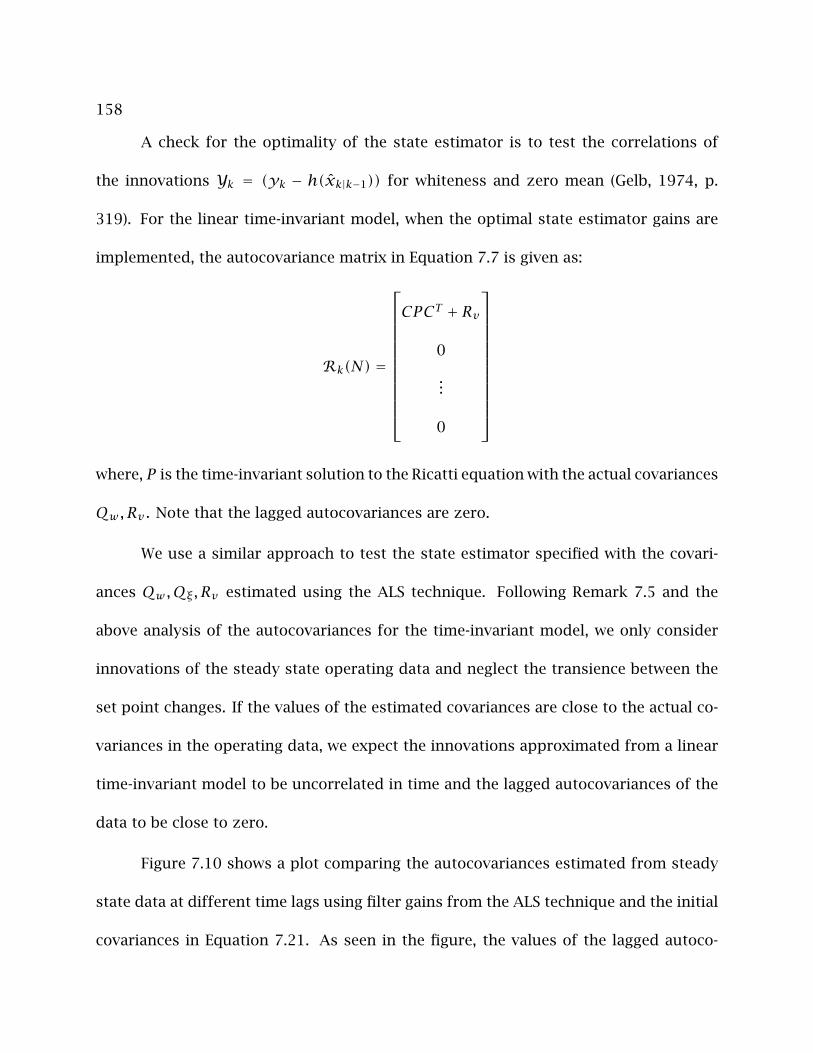
158

A check for the optimality of the state estimator is to test the correlations of

the innovations Yk = (yk − h(xk|k−1)) for whiteness and zero mean (Gelb, 1974, p.

319). For the linear time-invariant model, when the optimal state estimator gains are

implemented, the autocovariance matrix in Equation 7.7 is given as:

Rk(N) =

CPCT + Rv

0

...

0

where, P is the time-invariant solution to the Ricatti equation with the actual covariances

Qw , Rv . Note that the lagged autocovariances are zero.

We use a similar approach to test the state estimator specified with the covari-

ances Qw ,Qξ, Rv estimated using the ALS technique. Following Remark 7.5 and the

above analysis of the autocovariances for the time-invariant model, we only consider

innovations of the steady state operating data and neglect the transience between the

set point changes. If the values of the estimated covariances are close to the actual co-

variances in the operating data, we expect the innovations approximated from a linear

time-invariant model to be uncorrelated in time and the lagged autocovariances of the

data to be close to zero.

Figure 7.10 shows a plot comparing the autocovariances estimated from steady

state data at different time lags using filter gains from the ALS technique and the initial

covariances in Equation 7.21. As seen in the figure, the values of the lagged autoco-

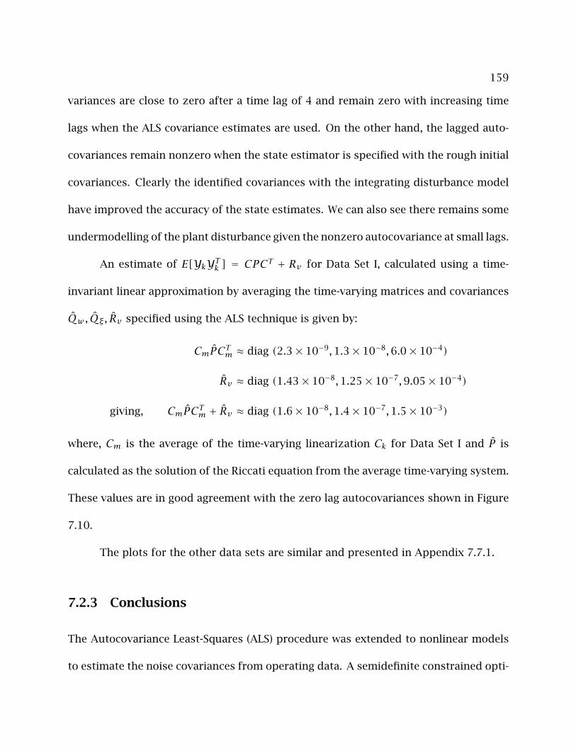
159

variances are close to zero after a time lag of 4 and remain zero with increasing time

lags when the ALS covariance estimates are used. On the other hand, the lagged auto-

covariances remain nonzero when the state estimator is specified with the rough initial

covariances. Clearly the identified covariances with the integrating disturbance model

have improved the accuracy of the state estimates. We can also see there remains some

undermodelling of the plant disturbance given the nonzero autocovariance at small lags.

An estimate of E[YkYTk ] = CPCT + Rv for Data Set I, calculated using a time-

invariant linear approximation by averaging the time-varying matrices and covariances

Qw , Qξ, Rv specified using the ALS technique is given by:

CmPCTm ≈ diag (2.3× 10−9,1.3× 10−8,6.0× 10−4)

Rv ≈ diag (1.43× 10−8,1.25× 10−7,9.05× 10−4)

giving, CmPCTm + Rv ≈ diag (1.6× 10−8,1.4× 10−7,1.5× 10−3)

where, Cm is the average of the time-varying linearization Ck for Data Set I and P is

calculated as the solution of the Riccati equation from the average time-varying system.

These values are in good agreement with the zero lag autocovariances shown in Figure

7.10.

The plots for the other data sets are similar and presented in Appendix 7.7.1.

7.2.3 Conclusions

The Autocovariance Least-Squares (ALS) procedure was extended to nonlinear models

to estimate the noise covariances from operating data. A semidefinite constrained opti-

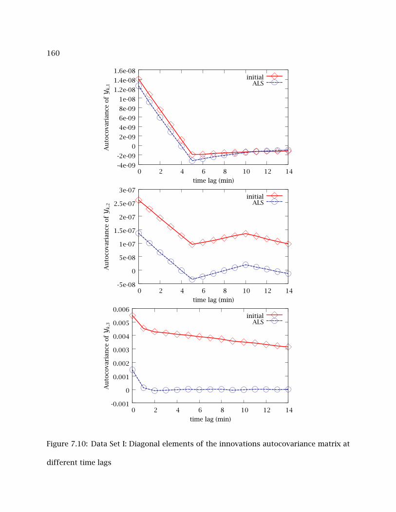
160

-4e-09

-2e-09

0

2e-09

4e-09

6e-09

8e-09

1e-08

1.2e-08

1.4e-08

1.6e-08

0 2 4 6 8 10 12 14

Au

toco

vari

ance

ofY k,1

time lag (min)

initialALS

-5e-08

0

5e-08

1e-07

1.5e-07

2e-07

2.5e-07

3e-07

0 2 4 6 8 10 12 14

Au

toco

vari

ance

ofY k,2

time lag (min)

initialALS

-0.001

0

0.001

0.002

0.003

0.004

0.005

0.006

0 2 4 6 8 10 12 14

Au

toco

vari

ance

ofY k,3

time lag (min)

initialALS

Figure 7.10: Data Set I: Diagonal elements of the innovations autocovariance matrix at

different time lags

161

mization with a least-squares objective was solved to give the covariance estimates. The

ALS technique was then shown to give good covariance estimates from data simulated

with known noise statistics. The practical benefits of the technique was illustrated by

an application to blending drum operating data sets provided by ExxonMobil Chemical

Company. Consistent values for the covariances were estimated in all the industrial

data sets provided by ExxonMobil Chemical Company. The state estimator specified

with covariances calculated using ALS technique produced white innovations implying

optimality in comparison to an initial choice for the covariances. The ALS technique

was also used to estimate the covariances for integrating output disturbance models

to remove the plant/model mismatch. The improvement in the estimator performance

implies cost benefits in the implementation of advanced control schemes (see for eg.

Odelson et al. (2006a) for numerical values) when the ALS technique is used to estimate

the noise covariances.

7.3 Connections between IDF and Using Integrating Input

Disturbance Models

Consider the plant to evolve according to the following continuous time nonlinear state-

space model:

x(t) = f(x(t),u(t))+ g(x(t),u(t))w

y(t) = h(x(t))+ v(7.22)

162

where x ∈ Rn is the state, u the input and y ∈ Rp the measurements. w and v are the

process and the measurement noises.

Given the history of measurements Yk = y0, y1, · · · , yk at times t0, t1, · · · , tk

and a model for the plant, we want to estimate the state of the system at time tk.

7.4 Implicit Dynamic Feedback (IDF)

Implicit Dynamic Feedback (IDF) is one of the current state estimation techniques used

in the chemical industry. IDF is also the state estimator used for the ethylene co-

polymerization reactor at ExxonMobil Chemical Company.

Let measurements be available at the discrete times t0, t1, · · · . When the mea-

surement at tk+1 becomes available, IDF estimates the disturbance variables as the fol-

lowing integral of the difference between the actual plant output and the model output

(Hedengren et al., 2007):

d(t | Yk+1) = K(yk+1 − y(t | Yk+1))+KτI

∫ t0(yk+1 − y(T | Yk+1))dT (7.23)

where, d(t | Yk+1) is the estimate of the disturbance given the history of the mea-

surements Yk. The estimate d(t | Yk+1) is calculated at every time instant between

tk < t < tk+1 after the measurement yk+1 becomes available. The predicted output

y(t | Yk+1) is obtained using the measurement model y = h(x) and by solving the

state equation simultaneously. K and τI are scalars chosen for each measurement in

163

the y vector. For example if the measurement vector is of size 3, then K is the matrix:K1 0 0

0 K2 0

0 0 K3

Each element from the estimated d vector is paired with a state of the system.

Examples of the pairings are: the measurement ethylene feed is paired with ethylene mol

% which is state variable and measured state catalyst activity is paired with the state

variable production rate.

The evolution of the IDF model over the time interval tk < t ≤ tk+1 is:

x(t) = f(x(t),uk)+ Bdd(t)

y(t) = h(x(t)), tk < t ≤ tk+1

x(tk) = xk|k

(7.24)

in which, Bd is the matrix containing the chosen pairings between the disturbance vector

d and the model states x. The input uk is held constant over the time interval. The

notation xk|k is used as a shorthand for x(tk | Yk).

Thus, to get the IDF state estimate, Equation 7.23 is solved simultaneously with

Equation 7.24:

x(t | Yk+1) = xk|k +∫ ttk[f (x(T),uk)+ Bdd(T)]dT , tk < t ≤ tk+1 (7.25)

Differentiating Equation 7.23 w.r.t time, we get:

δd(t | Yk+1)δt

= −K dhdx

∣∣∣∣x(t)[f (x(t),uk)+ Bdd(t)]+

KτI(yk+1 − h(x(t))) (7.26)

164

Thus, to get to IDF state estimates in the time interval tk < t ≤ tk+1, after the

measurement yk+1 is available, the following set of differential equations have to solved

simultaneously:

δx(t | Yk+1)δt

= f(x(t),uk)+ Bdd(t)

δd(t | Yk+1)δt

= −K dhdx

∣∣∣∣x(t)[f (x(t),uk)+ Bdd(t)]+

KτI(yk+1 − h(x(t)))

subject to initial conditions,

x(tk) = xk|k

d(tk) = dk|k

(7.27)

7.5 Equivalence between integrating disturbance models

and IDF for discrete-time systems

For purposes of illustrating the equivalence between integrating disturbances and IDF,

we consider the following linear state-space model:


yk = Cxk + vk(7.28)

The more general nonlinear, continuous time case is considered briefly in Section 7.5.3.

165

7.5.1 Input Disturbance Models

To prevent offset in the outputs, model predictive control (MPC) includes integrating

disturbance models to account for plant/model mismatch. The integrating disturbance

is either added to the input or the output (Pannocchia and Rawlings, 2002). In this

report we show the equivalence of IDF and the integrating input disturbance model.

The dynamics of the integrating white noise is included in the state-space model

by augmenting the state vector with the disturbance vector m. The state-space model

with the integrating disturbance added to the input is then given by:xm

k+1

=

A Bd

0 I

xm

k

+

B0

uk +G 0

0 I

wξ

k

yk =[C 0

]xm

k

+ vk

(7.29)

Bd models the integrating disturbance m entering the state. The optimal state esti-

mator for this linear augmented model with no constraints is the Kalman filter. If

wk ∼ N(0,Qw), vk ∼ N(0, Rv) and ξk ∼ N(0,Qξ) and the covariances Qw , Rv ,Qξ are

known parameters, then the Kalman filter gains Lx, Ld for the state and the disturbance

respectively can be easily calculated (Anderson and Moore, 1979).

The prediction equation is then: xm

k+1|k

=

A Bd

0 I

xm

k|k

+

B0

uk (7.30)

166

When the measurement yk+1 becomes available, the states are updated using the

Kalman filter gains (let εk = (yk − yk|k−1) = (yk − Cxk|k−1)): xm

k+1|k+1

=

xm

k+1|k

+

LxLd

εk+1 (7.31)

Writing the Kalman prediction and update equations in one step, we get: xm

k+1|k+1

=

A Bd

0 I

xm

k|k

+

B0

uk +ALx + BdLd

Ld

εk+1 (7.32)

7.5.2 IDF for discrete-time models

The continuous time IDF described in section 7.4 is implemented for the discrete-time

linear model shown in Equation 7.28. If the discretization time is ∆t, then an approxi-

mation of Equation 7.23 is (εk = (yk − yk|k−1)):

dk+1|k+1 = Kεk+1 +αk+1∑j=0

εj (7.33)

where,

α = K∆tτI

Equation 7.33 can be written as:

dk+1|k+1 = (K +α)εk+1 +αk∑j=0

εj

Define:

nk|k = αk∑j=0

εj (7.34)

167

We get,

dk+1|k+1 = (K +α)εk+1 + nk|k

nk|k = nk−1|k−1 +αεk(7.35)

The IDF state estimate for the discrete linear model similar to Equation 7.27 is

given by:

xk+1|k+1 = Axk|k + Buk + Bddk+1|k+1

Using Equation 7.35,

xk+1|k+1 = Axk|k + Buk + Bd(K +α)εk+1 + Bdnk|k (7.36)

Thus, from Equations 7.35 and 7.36, we get:xn

k+1|k+1

=

A Bd

0 I

xn

k|k

+

B0

uk +BdK + Bdα

α

εk+1 (7.37)

Comparing the Kalman filter in Equation 7.32 and the IDF in Equation 7.37, we see

thatnk defined in Equation 7.34 takes the role of the integrating white noise disturbance

dk added to the inputs and Bd is the equivalent of Bd in the input disturbance model.

Also, we the have the following relationships:

α = Ld

BdK + Bdα = ALx + BdLd(7.38)

Thus, if we estimate the Kalman filter gain from data using the ALS techniques given in

Chapter 5 and impose a particular structure on the filter gain estimate, we can calculate

the equivalent IDF estimator gain.

168

7.5.3 IDF on Continuous time systems

When the model is nonlinear and in continuous time, an approach similar to Section 7.5

can be taken for implementing the IDF in the form of a Kalman filter.

Consider the state propagation model to be nonlinear and in continuous time.

The measurements are obtained at discrete times. The model then has the following

form:

System Model: x(t) = f(x(t), t)+ g(x(t))w

Measurement Model: yk = hk(x(tk))+ vk

The state estimation in this case is achieved by implementing a continuous-

discrete linearized Kalman filter (Gelb, 1974, p.189). An equivalence between IDF and

the continuous-discrete Kalman filter can again been shown using a derivation similar

to the previous section.

7.5.4 Conclusions

It was shown that IDF is a special case of the Kalman filter applied to integrating input

disturbance models in MPC. This equivalence motivates using the ALS technique to

specify the covariances for the IDF implementation.

169

7.6 Using ALS with Shell Multivariable Optimization Con-

trol (SMOC)

The implementation of Shell’s SMOC strategy includes an integrating disturbance model

with a structure described in Section 7.6.1 to allow more flexibility in removing offset

in the presence of unmodelled disturbances and plant/model mismatch. In this section

we show that the special disturbance model structure in SMOC is a particular choice for

the structures of Bd and Cd. Also as shown in Chapter 5, the ALS technique can be used

to estimate the covariances that specify the state estimator for the SMOC disturbance

structure and achieve a closed-loop performance equivalent to other detectable choices

for Bd and Cd, also with an ALS specified estimator.

7.6.1 Model Description

Figure 7.11 is a schematic diagram showing the structure of the disturbance models

implemented in SMOC. Referring to the model shown in Figure 7.11, the state-space

models can be written as the following equations: For the first block:

x1(k+ 1) = A1x1(k)+ B1u1(k)

y1(k) = C1x1(k)+ d1(k)+D1u1(k)(7.39)

For the second block:

x2(k+ 1) = A2x2(k)+ B2u2(k)

x4(k) = C2x2(k)+D2u2(k)(7.40)

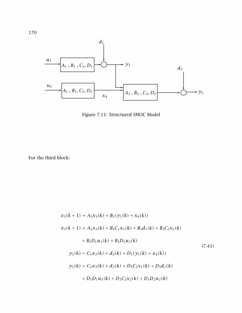
170

y2

d2

u1

u2A2 , B2, C2, D2

x4

d1

A3 , B3 , C3, D3

A1 , B1 , C1, D1 y1

Figure 7.11: Structured SMOC Model

For the third block:

x3(k+ 1) = A3x3(k)+ B3(y1(k)+ x4(k))

x3(k+ 1) = A3x3(k)+ B3C1x1(k)+ B3d1(k)+ B3C2x2(k)

+ B3D1u1(k)+ B3D2u2(k)

y2(k) = C3x3(k)+ d2(k)+D3(y1(k)+ x4(k))

y2(k) = C3x3(k)+ d2(k)+D3C1x1(k)+D3d1(k)

+D3D1u1(k)+D3C2x2(k)+D3D2u2(k)

(7.41)

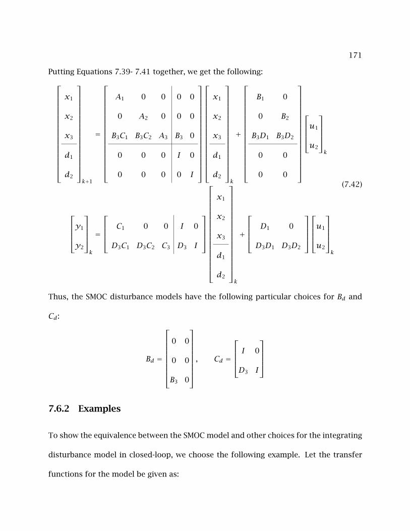
171

Putting Equations 7.39- 7.41 together, we get the following:

x1

x2

x3

d1

d2

k+1

=

A1 0 0 0 0

0 A2 0 0 0

B3C1 B3C2 A3 B3 0

0 0 0 I 0

0 0 0 0 I

x1

x2

x3

d1

d2

k

+

B1 0

0 B2

B3D1 B3D2

0 0

0 0

u1

u2

k

y1

y2

k

=

C1 0 0 I 0

D3C1 D3C2 C3 D3 I

x1

x2

x3

d1

d2

k

+

D1 0

D3D1 D3D2

u1

u2

k

(7.42)

Thus, the SMOC disturbance models have the following particular choices for Bd and

Cd:

Bd =

0 0

0 0

B3 0

, Cd =

I 0

D3 I

7.6.2 Examples

To show the equivalence between the SMOC model and other choices for the integrating

disturbance model in closed-loop, we choose the following example. Let the transfer

functions for the model be given as:

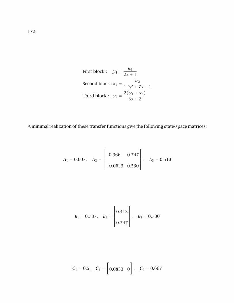
172

First block : y1 =u1

2s + 1

Second block :x4 =u2

12s2 + 7s + 1

Third block : y2 =2(y1 + x4)

3s + 2

A minimal realization of these transfer functions give the following state-space matrices:

A1 = 0.607, A2 =

0.966 0.747

−0.0623 0.530

, A3 = 0.513

B1 = 0.787, B2 =

0.413

0.747

, B3 = 0.730

C1 = 0.5, C2 =[

0.0833 0

], C3 = 0.667

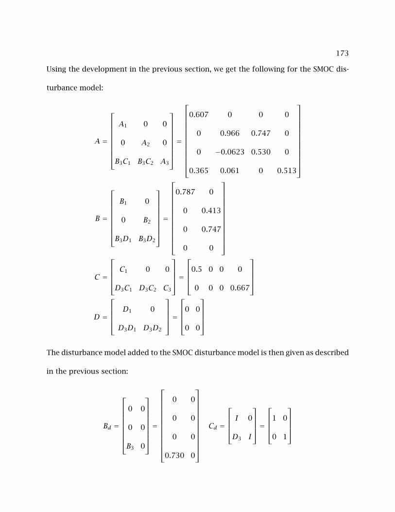
173

Using the development in the previous section, we get the following for the SMOC dis-

turbance model:

A =

A1 0 0

0 A2 0

B3C1 B3C2 A3

=

0.607 0 0 0

0 0.966 0.747 0

0 −0.0623 0.530 0

0.365 0.061 0 0.513

B =

B1 0

0 B2

B3D1 B3D2

=

0.787 0

0 0.413

0 0.747

0 0

C =

C1 0 0

D3C1 D3C2 C3

=0.5 0 0 0

0 0 0 0.667

D =

D1 0

D3D1 D3D2

=0 0

0 0

The disturbance model added to the SMOC disturbance model is then given as described

in the previous section:

Bd =

0 0

0 0

B3 0

=

0 0

0 0

0 0

0.730 0

Cd =

I 0

D3 I

=1 0

0 1

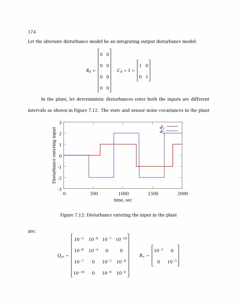
174

Let the alternate disturbance model be an integrating output disturbance model:

Bd =

0 0

0 0

0 0

0 0

Cd = I =

1 0

0 1

In the plant, let deterministic disturbances enter both the inputs are different

intervals as shown in Figure 7.12. The state and sensor noise covariances in the plant

-3

-2

-1

0

1

2

3

0 500 1000 1500 2000

Dis

turb

ance

ente

rin

gin

pu

t

time, sec

d1d2

Figure 7.12: Disturbance entering the input in the plant

are:

Qw =

10−5 10−8 10−7 10−10

10−8 10−4 0 0

10−7 0 10−5 10−8

10−10 0 10−8 10−6

Rv =

10−5 0

0 10−5

175

Using the closed-loop data from the plant, with the estimator specified with arbitrary

covariances (initial filter gain Li) , the autocovariance least-squares (ALS) technique is

used to find the new Kalman filter gain (say, Lo) for the output disturbance model. Note

that in SMOC the disturbance is modelled as entering partly in the input and partly in

the output.

If the model had the SMOC structure, then a transformation can be calculated

(provided condition given in Chapter 5 are satisfied) from the output disturbance model

to this SMOC model, such that the corresponding filter gain for the SMOC model can be

calculated knowing Lo. This SMOC model with estimator gain: Ls then gives the same

closed-loop performance (same inputs and outputs) as the output disturbance model

with Lo

For the particular model in the example, the transformation matrix is uniquely

calculated as:

T =

1 0 0 0 0 0

0 1 0 0 0 0

0 0 1 0 0 0

0 0 0 1 1.5 0

0 0 0 0 1 0

0 0 0 0 −1 1

and the corresponding SMOC filter gain is then Ls = TLo.

For the purpose of comparison, the L estimated from data using the ALS technique

for the SMOC model is presented in Table 7.1. The performances for the three cases

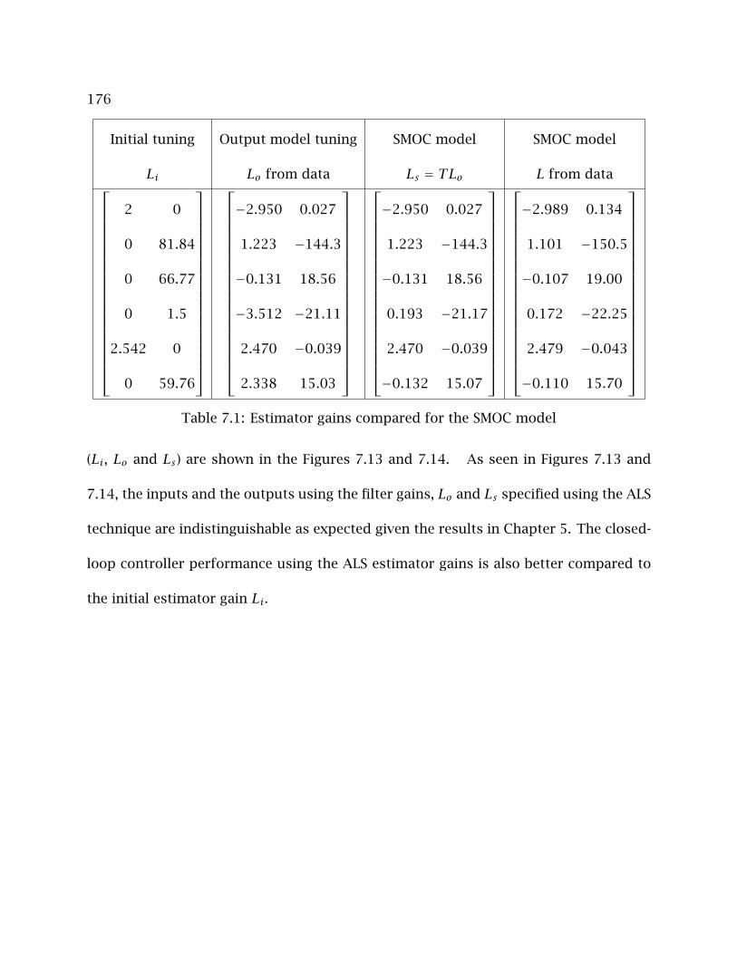
176

Initial tuning Output model tuning SMOC model SMOC model

Li Lo from data Ls = TLo L from data

2 0

0 81.84

0 66.77

0 1.5

2.542 0

0 59.76

−2.950 0.027

1.223 −144.3

−0.131 18.56

−3.512 −21.11

2.470 −0.039

2.338 15.03

−2.950 0.027

1.223 −144.3

−0.131 18.56

0.193 −21.17

2.470 −0.039

−0.132 15.07

−2.989 0.134

1.101 −150.5

−0.107 19.00

0.172 −22.25

2.479 −0.043

−0.110 15.70

Table 7.1: Estimator gains compared for the SMOC model

(Li, Lo and Ls) are shown in the Figures 7.13 and 7.14. As seen in Figures 7.13 and

7.14, the inputs and the outputs using the filter gains, Lo and Ls specified using the ALS

technique are indistinguishable as expected given the results in Chapter 5. The closed-

loop controller performance using the ALS estimator gains is also better compared to

the initial estimator gain Li.

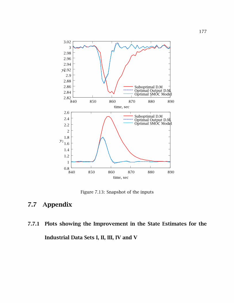
177

2.82

2.84

2.86

2.88

2.9

2.92

2.94

2.96

2.98

3

3.02

840 850 860 870 880 890

time, sec

y1

Suboptimal D.MOptimal Output D.M.Optimal SMOC Model

0.8

1

1.2

1.4

1.6

1.8

2

2.2

2.4

2.6

840 850 860 870 880 890

time, sec

y2

Suboptimal D.MOptimal Output D.M.Optimal SMOC Model

Figure 7.13: Snapshot of the inputs

7.7 Appendix

7.7.1 Plots showing the Improvement in the State Estimates for the

Industrial Data Sets I, II, III, IV and V

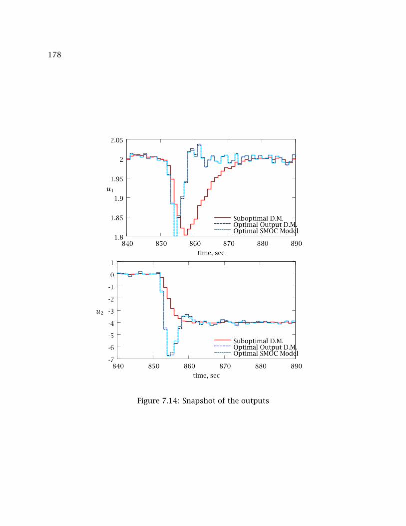
178

1.8

1.85

1.9

1.95

2

2.05

840 850 860 870 880 890

time, sec

u1

Suboptimal D.M.Optimal Output D.M.Optimal SMOC Model

-7

-6

-5

-4

-3

-2

-1

0

1

840 850 860 870 880 890

time, sec

u2

Suboptimal D.M.Optimal Output D.M.Optimal SMOC Model

Figure 7.14: Snapshot of the outputs

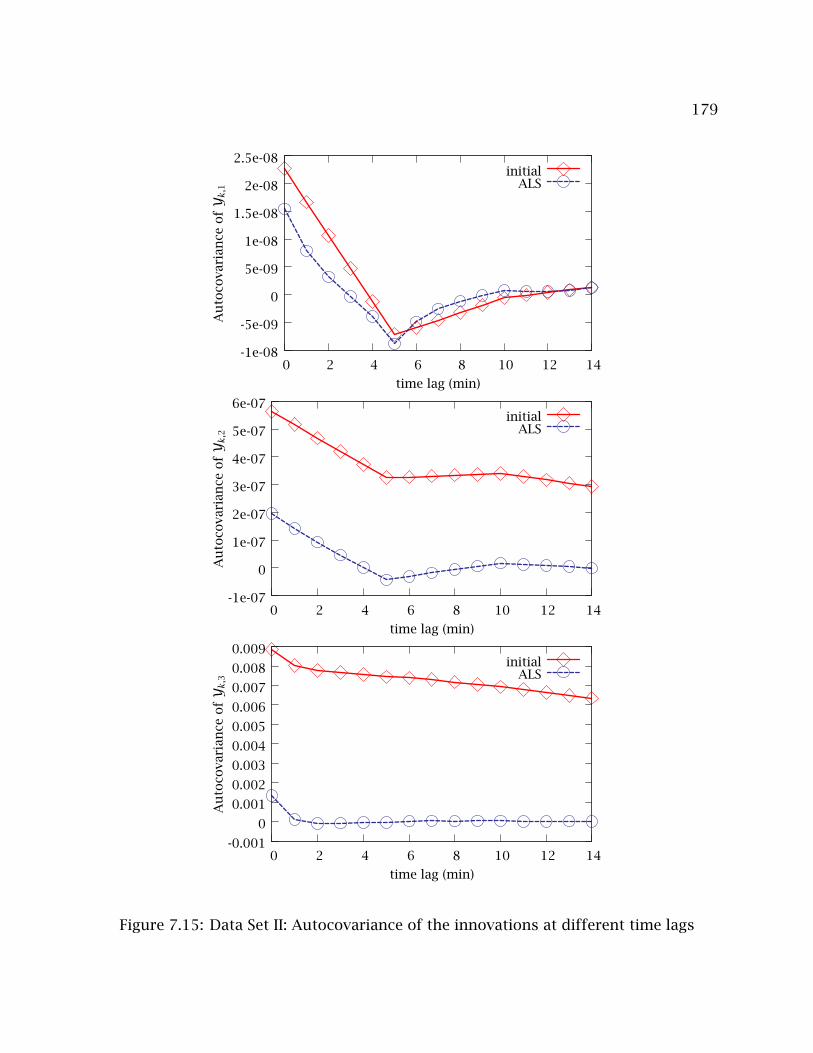
179

-1e-08

-5e-09

0

5e-09

1e-08

1.5e-08

2e-08

2.5e-08

0 2 4 6 8 10 12 14

Au

toco

vari

ance

ofY k,1

time lag (min)

initialALS

-1e-07

0

1e-07

2e-07

3e-07

4e-07

5e-07

6e-07

0 2 4 6 8 10 12 14

Au

toco

vari

ance

ofY k,2

time lag (min)

initialALS

-0.001

0

0.001

0.002

0.003

0.004

0.005

0.006

0.007

0.008

0.009

0 2 4 6 8 10 12 14

Au

toco

vari

ance

ofY k,3

time lag (min)

initialALS

Figure 7.15: Data Set II: Autocovariance of the innovations at different time lags

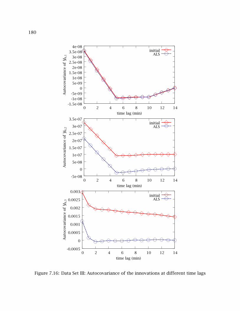
180

-1.5e-08-1e-08-5e-09

05e-091e-08

1.5e-082e-08

2.5e-083e-08

3.5e-084e-08

0 2 4 6 8 10 12 14

Au

toco

vari

ance

ofY k,1

time lag (min)

initialALS

-5e-08

0

5e-08

1e-07

1.5e-07

2e-07

2.5e-07

3e-07

3.5e-07

0 2 4 6 8 10 12 14

Au

toco

vari

ance

ofY k,2

time lag (min)

initialALS

-0.0005

0

0.0005

0.001

0.0015

0.002

0.0025

0.003

0 2 4 6 8 10 12 14

Au

toco

vari

ance

ofY k,3

time lag (min)

initialALS

Figure 7.16: Data Set III: Autocovariance of the innovations at different time lags

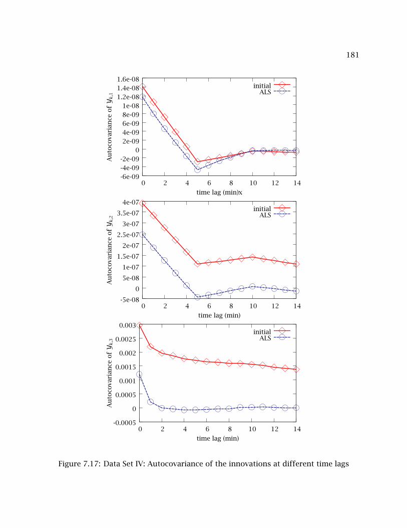
181

-6e-09-4e-09-2e-09

02e-094e-096e-098e-091e-08

1.2e-081.4e-081.6e-08

0 2 4 6 8 10 12 14

Au

toco

vari

ance

ofY k,1

time lag (min)x

initialALS

-5e-08

0

5e-08

1e-07

1.5e-07

2e-07

2.5e-07

3e-07

3.5e-07

4e-07

0 2 4 6 8 10 12 14

Au

toco

vari

ance

ofY k,2

time lag (min)

initialALS

-0.0005

0

0.0005

0.001

0.0015

0.002

0.0025

0.003

0 2 4 6 8 10 12 14

Au

toco

vari

ance

ofY k,3

time lag (min)

initialALS

Figure 7.17: Data Set IV: Autocovariance of the innovations at different time lags

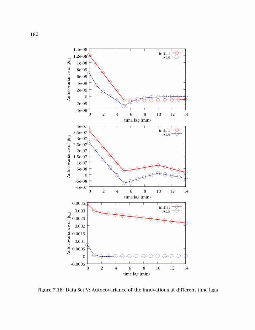
182

-4e-09

-2e-09

0

2e-09

4e-09

6e-09

8e-09

1e-08

1.2e-08

1.4e-08

0 2 4 6 8 10 12 14

Au

toco

vari

ance

ofY k,1

time lag (min)

initialALS

-1e-07

-5e-08

0

5e-08

1e-07

1.5e-07

2e-07

2.5e-07

3e-07

3.5e-07

4e-07

0 2 4 6 8 10 12 14

Au

toco

vari

ance

ofY k,2

time lag (min)

initialALS

-0.0005

0

0.0005

0.001

0.0015

0.002

0.0025

0.003

0.0035

0 2 4 6 8 10 12 14

Au

toco

vari

ance

ofY k,3

time lag (min)

initialALS

Figure 7.18: Data Set V: Autocovariance of the innovations at different time lags

183

Chapter 8

Other Nonlinear State Estimation

Techniques : Hybrid of Particle Filters

and Moving Horizon Estimation 1

8.1 Introduction

Most processes in the chemical industry exhibit nonlinear dynamics and efficient nonlin-

ear state estimators are an active area of research. The accuracy of the state estimates is

important in advanced process control and the performance of a closed-loop controller

is directly affected by the quality of the current state estimate. Some state estimators

for nonlinear models are Extended Kalman Filters (EKF) (Lee and Ricker, 1994; Myers

and Luecke, 1991; Haseltine and Rawlings, 2005; Reif et al., 1999), Moving Horizon Esti-

1Portions of this chapter appear in Rajamani and Rawlings (2007)

184

mators (MHE) (Rao et al., 2003; Robertson et al., 1996), Unscented Kalman Filters (UKF)

(Julier et al., 2000; Julier and Uhlmann, 2004a,b; Wu et al., 2004) and the Particle Filters

(PF) (Doucet et al., 2000; Arulampalam et al., 2002; Rawlings and Bakshi, 2006; Kotecha

and Djuric, 2003). Although the EKF has been the most popular in the chemical in-

dustry, the performance of the EKF has been criticized in the literature due to the lack

of theoretical convergence properties and lack of accuracy in the state estimates when

applied to significantly nonlinear models. The unscented Kalman filter is the Kalman

filter based on the unscented transformation and was largely pioneered by Julier et al.

(2000). The UKF as an alternative to the extended Kalman filter has been studied on sev-

eral applications eg. Romanenko and Castro (2004); Romanenko et al. (2004); Sitz et al.

(2004). The UKF unlike the EKF satisfies convergence properties and the approximation

of the model is exact up to the second order. The UKF however, lacks the robustness

offered by optimization based state estimators like the moving horizon estimator.

In this chapter, we present a new state hybrid estimator combining the Moving

Horizon Estimator (MHE) and the Particle Filter (PF). The advantages of optimizing over

a trajectory of states estimates as implemented in the MHE and the computational speed

of the PF, combine to give a fast yet robust hybrid estimator. In Section 8.2 state esti-

mation applied to nonlinear models is introduced and the MHE and PF techniques are

presented in Sections 8.2.1 and 8.2.2 respectively. We next describe the MHE/PF hy-

brid technique in Section 8.2.3 and present the results of an application in Section 8.3.

Finally, the conclusions are given in Section 8.4.

185

8.2 Nonlinear State Estimation

Consider the nonlinear discrete-time state-space model given in Chapter 7:

xk+1 = f(xk, uk)+ g(xk, uk)wk

yk = h(xk)+ vk(8.1)

where, wk and vk are the state and the measurement noises drawn from the Gaussian

distributions N(0,Qw) and N(0, Rv) respectively. The restriction on the noises wk, vk

being drawn from the Gaussian distribution is not restricting and considered here for

simplicity. Given the above system model, at any given time tk, the measurements

y0:k = y0, y1 · · ·yk and the inputs u0:k = u0, u1, · · ·uk are available. Here and

in the sequel, we use x0:k, u0:k and y0:k as shorthand notations for the trajectories of

xk, uk and yk respectively. Mathematically, the optimal state estimate xk for the state

at time tk is then defined as:

xk = arg maxxkp(xk|y0:k) (8.2)

subject to state constraints, the given inputs Uk and the nonlinear model in Equation

8.1.

A closed form analytical solution for Equation 8.2 is usually not available except

for the simplest of cases. For the linear model with no constraints and Gaussian distri-

butions forwk, vk, Equation 8.2 gives the classical Kalman filter recursion. For nonlinear

models, such a simplification is usually not possible. When we have non-Gaussian dis-

tributions for wk, vk, multi-modality of the state estimates or bad guesses for x0, the

problem of finding the state estimates by solving Equation 8.2 is even more difficult.

186

8.2.1 Moving Horizon Estimation

Moving horizon estimation (MHE) is an optimization based state estimator, which makes

it convenient to handle constraints. In MHE, the optimization variables are the state

trajectory over a past horizon of length N rather than just the current state as with EKF,

UKF and the PF. The following optimization is then solved as opposed to Equation 8.2:

maxxk−N:k

p(xk−N:k|y0:k) (8.3)

subject to state constraints, the given inputs u0:k and Equation 8.1.

Using the trajectory of states over a past horizon provides robustness against bad

data, outliers, bad priors and unmodelled disturbances. If the horizon length is N and

the noiseswk, vk are from the Gaussian distributionswk ∼ N(0,Qw) and vk ∼ N(0, Rv),

the MHE optimization in Equation 8.3 reduces to (Tenny, 2002; Haseltine, 2005):

minxk−N ,···xk

(xk−N − xk−N)TP−1k−N(xk−N − xk−N)+

N−1∑i=0

wTk−iQ−1w wk−i + vTk−iR−1

v vk−i

subject to, xk+1 = f(xk, uk)+ g(xk, uk)wk

yk = h(xk)+ vk

xk−N , · · · xk ∈ X

(8.4)

where, X is the constraint set for the states and xk−N and Pk−N are the mean and the

covariance of the approximated Gaussian distribution of the state xk−N . The perfor-

mance of the MHE depends on the horizon N and the choice of the approximations for

the prior xk−N and Pk−N . The choice for the weight Pk−N is such that it gives a good ap-

187

proximation of the past data that not included in the horizon. For more details on the

choice of xk−N and Pk−N see Rao et al. (2003). For the unconstrained linear model and

N chosen as the full length of data, the optimization in (8.4) simplifies to the Kalman

filter equations. The MHE solves an expensive nonlinear optimization at every time step

however, and may not be practical to implement in real time for many nonlinear and

large-dimensional applications.

8.2.2 Particle Filters

Particle filter is a sampling based approach to state estimation. The ideal sampling based

state estimator is one that samples the full posterior probability density p(x0:k|y0:k)

with large number of samples. If x(i)0:k with i = 1, · · · , s denotes s samples of the tra-

jectory x0:k and drawn from the distribution: p(x(i)0:k|y0:k), then the marginal p(xk|y0:k)

is approximated as the following sampled density:

p(xk|y0:k) ≈s∑i=1

W (i)k δ(x

(i)k − xk) (8.5)

where, the weights associated with x(i)k are chosen as W (i)k = 1/s and δ represents the

Delta function. This sampled density of the marginal from Equation 8.5 can then be

used to calculate the current state estimate as:

xk = E[xk|y0:k] =∫xkp(xk|y0:k)dxk ≈

s∑i=1

W (i)k x

(i)k (8.6)

However, the full posterior density p(x0:k|y0:k) is not available for sampling in most

nonlinear cases and the sample and weight pairs cannot be generated as easily as above.

188

To avoid this issue, samples are drawn from a different distribution called the Impor-

tance Function, denoted by π(x0:k|y0:k). The samples x(i)0:k are then associated with the

following weights, followed by a normalization step:

W∗(i)0:k = p(x

(i)0:k|y0:k)

π(x(i)0:k|y0:k), W (i)

0:k =W∗(i)

0:k∑si=1W

∗(i)0:k

(8.7)

The sample and the weight pairs x(i)0:k,W(i)0:k then represent the sampled density of

the probability density p(x0:k|y0:k) (Geweke, 1989). In the limit of large samples, the

above sampled density converges to p(x0:k|y0:k) (Smith and Gelfand, 1992; Gelfand and

Smith, 1990). The rate of convergence depends on the choice of the importance function

π(x0:k|y0:k) and how closely it matches the density of interest p(x0:k|y0:k).

Since the above sampling procedure is not recursive in time, new samples have

to be drawn from the importance function at every time step. To simplify the sampling

procedure and to get a recursion in time, the importance function is chosen in the

literature, to satisfy the following property (Doucet et al., 2000; Arulampalam et al.,

2002):

π(x0:k|y0:k) = π(x0|y0)k∏i=1

π(xi|x0:i−1, y0:i)

The weights in Equation 8.7 can be rewritten using Markov chain properties of the

state-space model in Equation 8.1 and using the importance function property above,

as the following recursion:

W∗(i)k =W∗(i)

k−1

p(x(i)k |x(i)k−1)p(yk|x

(i)k )

π(x(i)k |x(i)0:k−1, y0:k)p(yk|y0:k−1)

189

Since the quantity p(yk|y0:k−1) in the denominator above is difficult to evaluate and is

independent of the random variables, this quantity is absorbed into the normalization

step and the above equation is written as:

W∗(i)k =W∗(i)

k−1


(i)k )

π(x(i)k |x(i)0:k−1, y0:k)

, W (i)k = W∗(i)

k∑si=1W

∗(i)k

Note that p(x(i)k |x(i)k−1) and p(yk|x(i)k ) are usually available as known functions from

Equation 8.1 and can be evaluated.

The particle filter (PF) uses the importance sampling recursion described above

and provides state estimates as given in Equation 8.6. The following steps describe

the PF algorithm starting from a prior distributed as x0 ∼ N(x0, P0). The particle fil-

ter (also called the sequential importance sampling procedure in the literature) is then

implemented with the following steps (Doucet et al., 2000; de Freitas et al., 2000; Aru-

lampalam et al., 2002):

1. Draw s samplesx(1)0 , x(2)0 · · ·x(s)0 from the Gaussian prior distributionx0 ∼ N(x0, P0)

and assign weightsW∗(i)0 = 1/s to each sample.

2. Draw samples for the next time step from the importance functionπ(x(i)k |x(i)k−1, y0:k).

For example, if the importance function is chosen as the state propagation Equa-

tion 8.1:

π(x(i)k |x(i)k−1, y0:k) = f(x(i)k−1, uk−1)+ g(x(i)k−1, uk−1)wk−1

then, s noise samples m(i)k−1 are drawn from the normal N(0,Qw), which is the

distribution of the state noise wk−1, and the samples for the next time step are

190

given as:

x(i)k = f(x(i)k−1, uk−1)+ g(x(i)k−1, uk−1)m

(i)k−1

3. Evaluate the weights associated with the samples x(i)k up to a normalizing constant

using the recursion:

W∗(i)k =W∗(i)

k−1


(i)k )

π(x(i)k |x(i)0:k−1, y0:k)

4. Normalize the weights:

W (i)k = W∗(i)

k∑si=1W

∗(i)k

5. Optionally, resample among the available samples to avoid divergence of the sam-

ples and repeat above steps for the next time step. The resampling procedure is

described in more details in Smith and Gelfand (1992).

The s sample and weight pairs x(i)k ,W(i)k generated by the PF algorithm above are then

used to give the state estimates using Equation 8.6 at each time step:

xk ≈s∑i=1

W (i)k x

(i)k

The two critical things that dictate the performance of the PF implemented as

above are the choice of the importance function and whether and how often resampling

occurs. As described in Doucet et al. (2000), the importance function that gives zero

variance in the conditional weights is called the optimal importance function and is

given byp(x(i)k |x(i)k−1, yk) (See Appendix 8.5.2 for a derivation). However, zero variance in

191

the conditional weights does not imply that the samples track the state perfectly as seen

in the example in Appendix 8.5.4. The optimal importance function p(x(i)k |x(i)k−1, yk)

has a closed form solution whenever the measurement in Equation 8.1 is linear. A

more common choice for the importance function is p(x(i)k |x(i)k−1). This is the simplest

importance function with the samples propagated through the state equation as seen in

the PF algorithm steps described above. Note however, the above importance function

does not depend on the measurements and hence the samples diverge whenever the

measurement noise covariance is small. Proposition 1 in Doucet et al. (2000) notes

that the unconditional variance of the weights increases with time for any choice of

the importance function. But as shown in Appendix 8.5.1, the statement proves the

increasing variance with time, for a different recursion and not for the particle filter

algorithm that is implemented as above.

Resampling is an ad-hoc choice that fixes the divergence of the samples (Smith

and Gelfand, 1992). The resampling procedure draws samples from the already exist-

ing sample locations by interpreting the weights associated with the existing samples as

discrete probabilities and resetting the resampled weights to 1/s. The result of resam-

pling is an increase in the number of samples having higher weights and a decrease in

the number samples having smaller weights. As seen in the example in Appendix 8.5.4,

the resampling step is required even when the optimal importance function is used to

propagate the samples.

Thus, for the particle to perform efficiently, we need a good choice of the im-

192

portance function and judicious resampling. The advantage of using the particle filter

as a state estimator is that the computation is fast and it is easy to code compared to

other methods. However, since the PF estimates only the current state at every time in-

stant as opposed to a trajectory of states, it does not provide robustness to unmodelled

disturbances as illustrated in the example in Section 8.3.

8.2.3 Combination of MHE with Particle Filters (PF)

To combine the advantages of the MHE and PF techniques, we propose a hybrid MHE/PF

technique that works as follows:

• Use the MHE optimization to locate/relocate the samples

• Use the PF to obtain fast state estimates between MHE optimizations

The proposed MHE/PF hybrid has the advantage of fast computation times and ro-

bustness to bad priors and unmodelled disturbances. The hybrid estimator offers an

advantage whenever the MHE optimization cannot be solved within the sampling time.

The hybrid MHE/PF provides a practical and implementable state estimator.

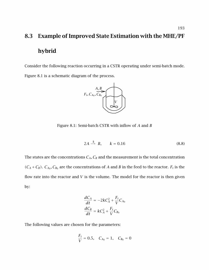
193

8.3 Example of Improved State Estimation with the MHE/PF

hybrid

Consider the following reaction occurring in a CSTR operating under semi-batch mode.

Figure 8.1 is a schematic diagram of the process.

V

A,BFi, CA0 , CB0

Figure 8.1: Semi-batch CSTR with inflow of A and B

2A k-→ B, k = 0.16 (8.8)

The states are the concentrations CA, CB and the measurement is the total concentration

(CA+CB). CA0 , CB0 are the concentrations of A and B in the feed to the reactor. Fi is the

flow rate into the reactor and V is the volume. The model for the reactor is then given

by:

dCAdt

= −2kC2A +

FiVCA0

dCBdt

= kC2A +

FiVCB0

The following values are chosen for the parameters:

FiV= 0.5, CA0 = 1, CB0 = 0

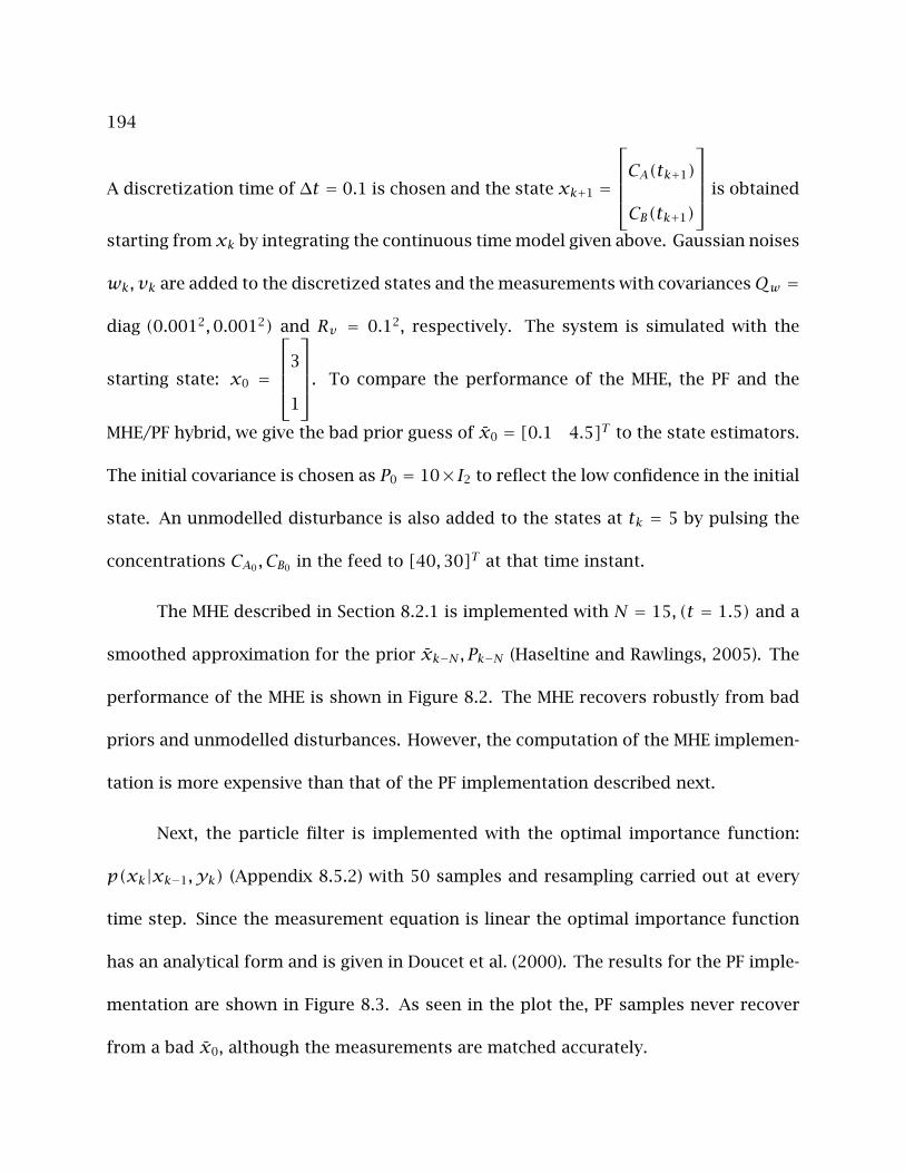
194

A discretization time of ∆t = 0.1 is chosen and the state xk+1 =

CA(tk+1)

CB(tk+1)

is obtained

starting from xk by integrating the continuous time model given above. Gaussian noises

wk, vk are added to the discretized states and the measurements with covariancesQw =

diag (0.0012,0.0012) and Rv = 0.12, respectively. The system is simulated with the

starting state: x0 =

3

1

. To compare the performance of the MHE, the PF and the

MHE/PF hybrid, we give the bad prior guess of x0 = [0.1 4.5]T to the state estimators.

The initial covariance is chosen as P0 = 10× I2 to reflect the low confidence in the initial

state. An unmodelled disturbance is also added to the states at tk = 5 by pulsing the

concentrations CA0 , CB0 in the feed to [40,30]T at that time instant.

The MHE described in Section 8.2.1 is implemented with N = 15, (t = 1.5) and a

smoothed approximation for the prior xk−N , Pk−N (Haseltine and Rawlings, 2005). The

performance of the MHE is shown in Figure 8.2. The MHE recovers robustly from bad

priors and unmodelled disturbances. However, the computation of the MHE implemen-

tation is more expensive than that of the PF implementation described next.

Next, the particle filter is implemented with the optimal importance function:

p(xk|xk−1, yk) (Appendix 8.5.2) with 50 samples and resampling carried out at every

time step. Since the measurement equation is linear the optimal importance function

has an analytical form and is given in Doucet et al. (2000). The results for the PF imple-

mentation are shown in Figure 8.3. As seen in the plot the, PF samples never recover

from a bad x0, although the measurements are matched accurately.

195

0

2

4

6

8

0 2 4 6 8 10 12

-2

0

2

4

6

8C

on

cen

trat

ion

s,CA,CB

Mea

sure

men

t,Y

time

CA

CB

Yestimates

Figure 8.2: MHE with a smoothing prior applied to the semi-batch reactor example

0

2

4

6

8

0 2 4 6 8 10 12

-2

0

2

4

6

8

Co

nce

ntr

atio

ns,CA,CB

Mea

sure

men

t,Y

time

CA

CB

Yestimates

Figure 8.3: PF with the optimal importance function applied to the semi-batch reactor

example

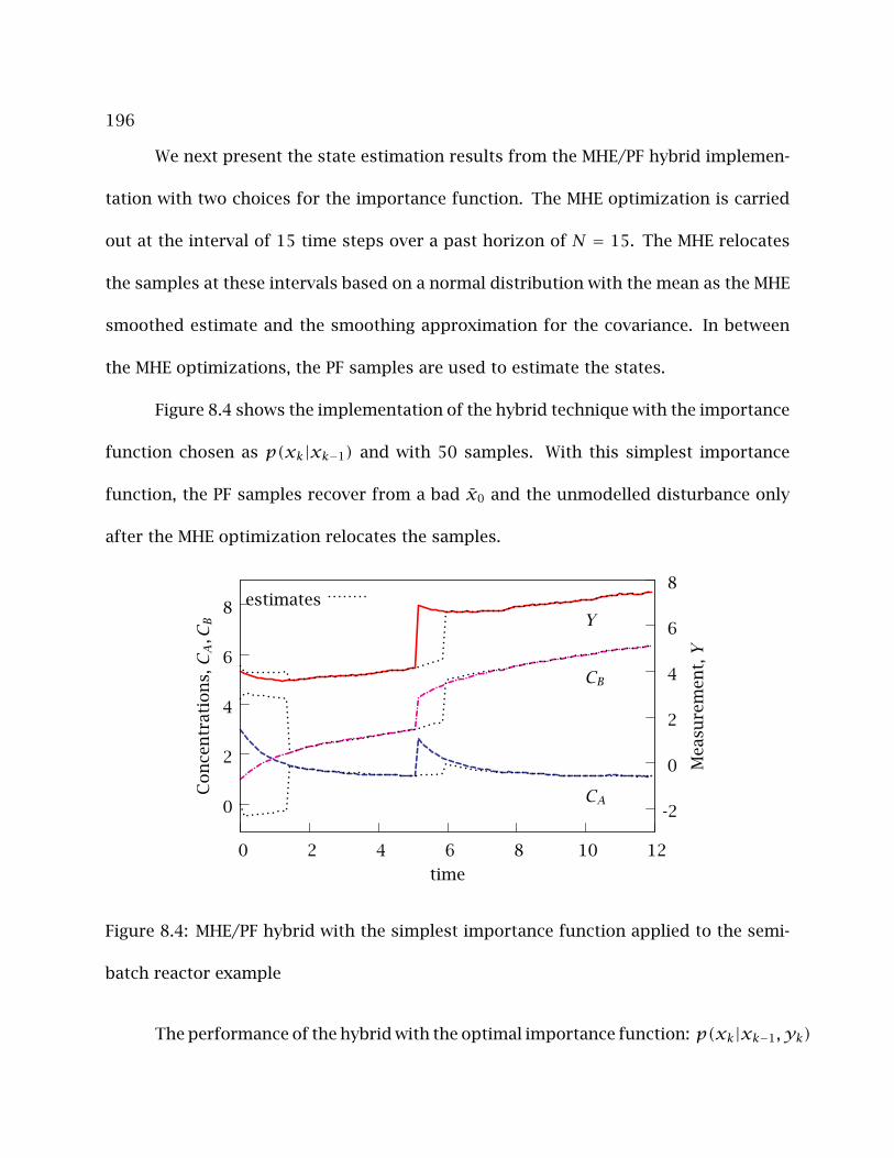
196

We next present the state estimation results from the MHE/PF hybrid implemen-

tation with two choices for the importance function. The MHE optimization is carried

out at the interval of 15 time steps over a past horizon of N = 15. The MHE relocates

the samples at these intervals based on a normal distribution with the mean as the MHE

smoothed estimate and the smoothing approximation for the covariance. In between

the MHE optimizations, the PF samples are used to estimate the states.

Figure 8.4 shows the implementation of the hybrid technique with the importance

function chosen as p(xk|xk−1) and with 50 samples. With this simplest importance

function, the PF samples recover from a bad x0 and the unmodelled disturbance only

after the MHE optimization relocates the samples.

0

2

4

6

8

0 2 4 6 8 10 12

-2

0

2

4

6

8

Co

nce

ntr

atio

ns,CA,CB

Mea

sure

men

t,Y

time

CA

CB

Yestimates

Figure 8.4: MHE/PF hybrid with the simplest importance function applied to the semi-

batch reactor example

The performance of the hybrid with the optimal importance function: p(xk|xk−1, yk)

197

and 50 samples is more interesting and is shown in Figure 8.5. As seen in the plot, the

MHE optimization is required to relocate the samples after a bad x0, but the samples

recover from the unmodelled disturbance without needing the MHE.

0

2

4

6

8

0 2 4 6 8 10 12

-2

0

2

4

6

8

Co

nce

ntr

atio

ns,CA,CB

Mea

sure

men

t,Y

time

CA

CB

Yestimates

Figure 8.5: MHE/PF hybrid with the optimal importance function applied to the semi-

batch reactor example

8.4 Conclusions to the Performance of the MHE/PF hybrid

To compare the performance of the MHE, the PF and the MHE/PF hybrid, we used the

following two tests:

Scenario 1: The initial valuex0 is proposed to come from the distributionN(x0, P0)

where x0 is incorrect and P0 is large to account for the low confidence in x0. The mea-

surement y0 is however, close to h(x0) where h(·) is the measurement equation.

198

Scenario 2: During normal operation, an unmodelled disturbance enters the pro-

cess at an intermediate time for a short time period. Since the model does not account

for this disturbance, the state estimates and the predicted measurements do not reflect

the actual system states and measurements at the time instance when the disturbance

occurs.

The performance of the MHE, the PF and the MHE/PF hybrid with two choices of

the importance function, under the above two Scenarios is described in the following

points:

1. MHE is implemented with the smoothed covariance estimate as the arrival cost.

• Under Scenario 1, MHE reliably fixes bad initial values of x0 whenever P0 is

large. A short horizon is enough to recover from the bad initial guess.

• Under Scenario 2, the performance of the MHE depends on the following

factors:

(a) The characteristics of the disturbance occurring and the covariances

chosen for Qw , Rv .

(b) The arrival cost approximation. If the arrival cost is too tight as with

the smoothed covariance estimate the MHE needs a large horizon to

overturn the prior.

(c) The horizon length N.

199

2. PF implemented with resampling and with the importance function chosen as

p(xk|xk−1).

• Fails under Scenario 1. The samples do not track either the state or the

measurement with bad values of x0.

• Fails under Scenario 2. The samples are unresponsive to unmodelled distur-

bances and do not track either state or the measurements.

3. PF implemented with resampling and with the optimal importance functionp(xk|xk−1, yk).

Note that a closed form for the optimal importance function is available only when

the measurement equation is linear.

• Can fix Scenario 1 with large number of samples, but is not reliable.

• Under Scenario 2, performance is similar to the MHE implemented with the

smoothed covariance as an approximation for the arrival cost.

4. The PF/MHE hybrid with resampling and the optimal importance function per-

forms better than either technique on its own in terms of accuracy and computa-

tion time.

Resampling is required when implementing the PF to prevent sampling of the state-

space that do not follow the measurements.

Overall, the MHE has more handles to fix Scenario 2 than the PF but at the cost of

additional computation time. The proposed MHE/PF hybrid on the other hand performs

200

robustly and provides a fix with both Scenarios. The MHE/PF hybrid also provides a

reliable state estimator that is implementable in real time. However, The performance

of the MHE/PF hybrid depends on the MHE computation time and the discretization

time. If the PF is a poor state estimator for a system, then the poor performance of the

MHE/PF hybrid scales with the time required to perform a MHE optimization.

201

8.5 Appendix

8.5.1 Proof of Proposition 1

Here, we prove Proposition 1 given in Doucet et al. (2000), where the claim is made that

the unconditional weights in the PF have an increasing variance.

The importance sampling weight recursion equation in the particle filter algo-

rithm is given as:

W∗(i)k =W∗(i)

k−1

p(yk|x(i)k )p(x(i)k |x

(i)k−1)

π(x(i)k |x(i)0:k−1, y0:k)

(8.9)

The unnormalized importance weight is defined as:

W∗(i)k = p(x

(i)0:k|y0:k)

π(x(i)0:k|y0:k)(8.10)

If π(x(i)0:k|y0:k) is chosen to satisfy:

π(x(i)0:k|y0:k) = π(x(i)0:k−1|y0:k−1)π(x(i)k |y0:k, x

(i)0:k−1) (8.11)

and the recursion on p(x(i)0:k|y0:k) gives (using Markov chain properties):

p(x(i)0:k|y0:k) =p(x(i)0:k−1|y0:k−1)p(yk|x(i)k p(x

(i)k |x

(i)k−1)

p(yk|y0:k−1)(8.12)

We then get,

W∗(i)k =W∗(i)

k−1


(i)k−1)

π(x(i)k |x(i)0:k−1, y0:k)p(yk|y0:k−1)

(8.13)

Note that this is not the same as the recursion given in Equation 8.9. Thep(yk|y0:k−1)

term in the denominator is ignored because it is assumed to be a constant.

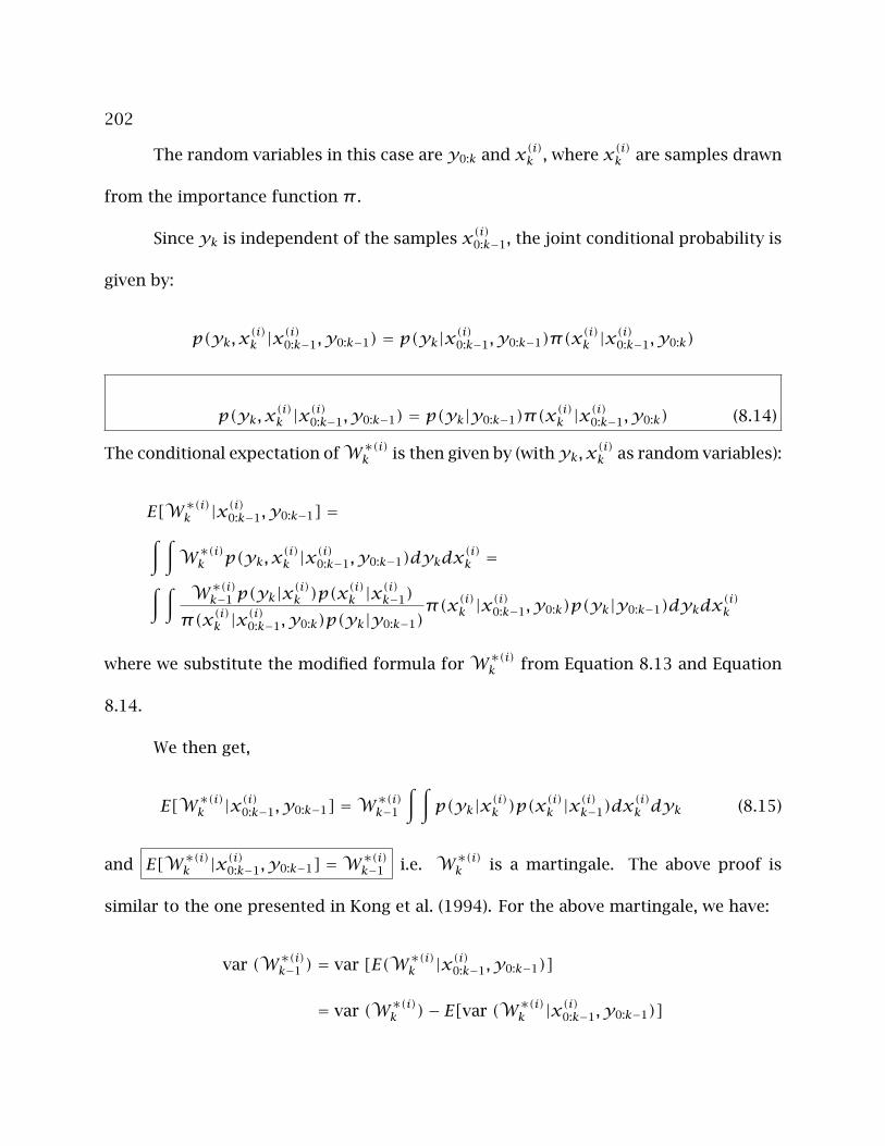
202

The random variables in this case are y0:k and x(i)k , where x(i)k are samples drawn

from the importance function π .

Since yk is independent of the samples x(i)0:k−1, the joint conditional probability is

given by:

p(yk, x(i)k |x

(i)0:k−1, y0:k−1) = p(yk|x(i)0:k−1, y0:k−1)π(x

(i)k |x

(i)0:k−1, y0:k)

p(yk, x(i)k |x

(i)0:k−1, y0:k−1) = p(yk|y0:k−1)π(x

(i)k |x

(i)0:k−1, y0:k) (8.14)

The conditional expectation ofW∗(i)k is then given by (withyk, x

(i)k as random variables):

E[W∗(i)k |x(i)0:k−1, y0:k−1] =∫ ∫W∗(i)k p(yk, x

(i)k |x

(i)0:k−1, y0:k−1)dykdx

(i)k =∫ ∫ W∗(i)

k−1 p(yk|x(i)k )p(x

(i)k |x

(i)k−1)

π(x(i)k |x(i)0:k−1, y0:k)p(yk|y0:k−1)

π(x(i)k |x(i)0:k−1, y0:k)p(yk|y0:k−1)dykdx

(i)k

where we substitute the modified formula for W∗(i)k from Equation 8.13 and Equation

8.14.

We then get,

E[W∗(i)k |x(i)0:k−1, y0:k−1] =W∗(i)

k−1

∫ ∫p(yk|x(i)k )p(x

(i)k |x

(i)k−1)dx

(i)k dyk (8.15)

and E[W∗(i)k |x(i)0:k−1, y0:k−1] =W∗(i)

k−1 i.e. W∗(i)k is a martingale. The above proof is

similar to the one presented in Kong et al. (1994). For the above martingale, we have:

var (W∗(i)k−1 ) = var [E(W∗(i)

k |x(i)0:k−1, y0:k−1)]

= var (W∗(i)k )− E[var (W∗(i)

k |x(i)0:k−1, y0:k−1)]

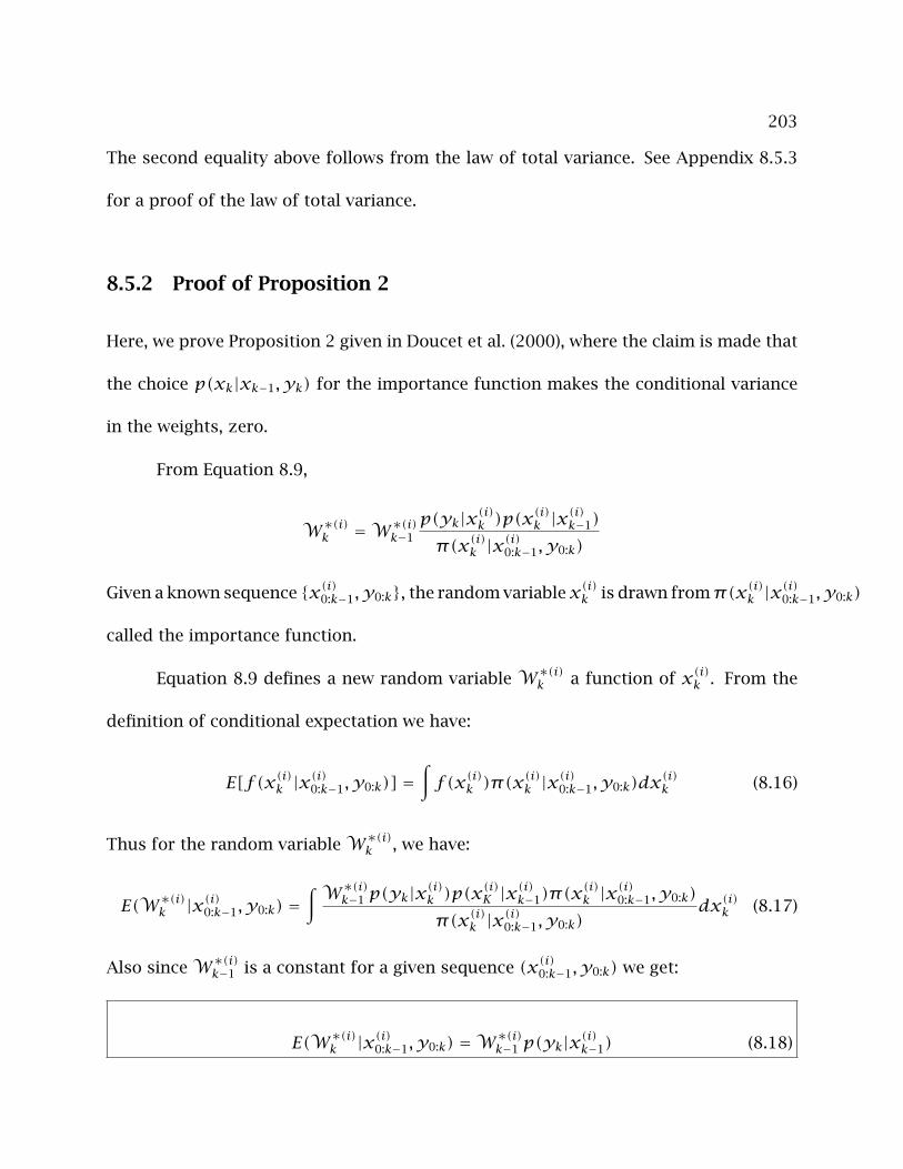
203

The second equality above follows from the law of total variance. See Appendix 8.5.3

for a proof of the law of total variance.

8.5.2 Proof of Proposition 2

Here, we prove Proposition 2 given in Doucet et al. (2000), where the claim is made that

the choice p(xk|xk−1, yk) for the importance function makes the conditional variance

in the weights, zero.

From Equation 8.9,

W∗(i)k =W∗(i)

k−1


(i)k−1)

π(x(i)k |x(i)0:k−1, y0:k)

Given a known sequence x(i)0:k−1, y0:k, the random variablex(i)k is drawn fromπ(x(i)k |x(i)0:k−1, y0:k)

called the importance function.

Equation 8.9 defines a new random variable W∗(i)k a function of x(i)k . From the

definition of conditional expectation we have:

E[f(x(i)k |x(i)0:k−1, y0:k)] =

∫f(x(i)k )π(x

(i)k |x

(i)0:k−1, y0:k)dx

(i)k (8.16)

Thus for the random variableW∗(i)k , we have:

E(W∗(i)k |x(i)0:k−1, y0:k) =

∫ W∗(i)k−1 p(yk|x

(i)k )p(x

(i)K |x(i)k−1)π(x

(i)k |x

(i)0:k−1, y0:k)

π(x(i)k |x(i)0:k−1, y0:k)

dx(i)k (8.17)

Also sinceW∗(i)k−1 is a constant for a given sequence (x(i)0:k−1, y0:k) we get:

E(W∗(i)k |x(i)0:k−1, y0:k) =W∗(i)

k−1 p(yk|x(i)k−1) (8.18)

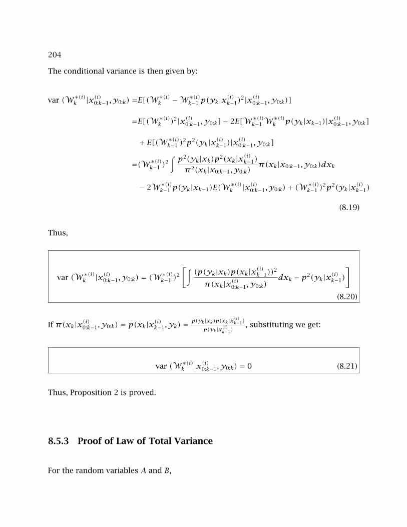
204

The conditional variance is then given by:

var (W∗(i)k |x(i)0:k−1, y0:k) =E[(W∗(i)

k −W∗(i)k−1 p(yk|x

(i)k−1)

2|x(i)0:k−1, y0:k)]

=E[(W∗(i)k )2|x(i)0:k−1, y0:k]− 2E[W∗(i)

k−1W∗(i)k p(yk|xk−1)|x(i)0:k−1, y0:k]

+ E[(W∗(i)k−1 )

2p2(yk|x(i)k−1)|x(i)0:k−1, y0:k]

=(W∗(i)k−1 )

2∫ p2(yk|xk)p2(xk|x(i)k−1)

π2(xk|x0:k−1, y0:k)π(xk|x0:k−1, y0:k)dxk

− 2W∗(i)k−1 p(yk|xk−1)E(W∗(i)

k |x(i)0:k−1, y0:k)+ (W∗(i)k−1 )

2p2(yk|x(i)k−1)

(8.19)

Thus,

var (W∗(i)k |x(i)0:k−1, y0:k) = (W∗(i)

k−1 )2

[∫ (p(yk|xk)p(xk|x(i)k−1))2

π(xk|x(i)0:k−1, y0:k)dxk − p2(yk|x(i)k−1)

](8.20)

If π(xk|x(i)0:k−1, y0:k) = p(xk|x(i)k−1, yk) =p(yk|xk)p(xk|x(i)k−1)

p(yk|x(i)k−1), substituting we get:

var (W∗(i)k |x(i)0:k−1, y0:k) = 0 (8.21)

Thus, Proposition 2 is proved.

8.5.3 Proof of Law of Total Variance

For the random variables A and B,

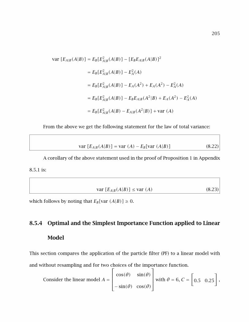
205

var [EA|B(A|B)] = EB[E2A|B(A|B)]− [EBEA|B(A|B)]2

= EB[E2A|B(A|B)]− E2

A(A)

= EB[E2A|B(A|B)]− EA(A2)+ EA(A2)− E2

A(A)

= EB[E2A|B(A|B)]− EBEA|B(A2|B)+ EA(A2)− E2

A(A)

= EB[E2A|B(A|B)− EA|B(A2|B)]+ var (A)

From the above we get the following statement for the law of total variance:

var [EA|B(A|B)] = var (A)− EB[var (A|B)] (8.22)

A corollary of the above statement used in the proof of Proposition 1 in Appendix

8.5.1 is:

var [EA|B(A|B)] ≤ var (A) (8.23)

which follows by noting that EB[var (A|B)] ≥ 0.

8.5.4 Optimal and the Simplest Importance Function applied to Linear

Model

This section compares the application of the particle filter (PF) to a linear model with

and without resampling and for two choices of the importance function.

Consider the linear model A =

cos(θ) sin(θ)

− sin(θ) cos(θ)

with θ = 6, C =[

0.5 0.25

],

206

B = I and G = I. The covariances are chosen as:

P0 =

1.75 1.25

1.25 1.75

, Qw = 0.01× I2, Rv = 0.01

The following inputs are provided to the model simulation for the first five time steps:

u1 = [7,2]T , u2 = [5,5]T , u3 = u4 = [−1,2]T , u5 = [1,−3]T

We first choose the simplest importance function given by p(xk|xk−1). For the

linear model this implies the samples are propagated using the state transition equa-

tion by drawing samples from the distribution N(0,Qw). Note that the propagation

of the samples does not depend on the measurements. Figures 8.6 and 8.7 show the

propagation of the samples with and without resampling with the simplest importance

function. As seen in the plots, the samples start diverging with time and do not track

the conditional densities accurately. Resampling fixes the divergence and the brings the

samples back to more reasonable locations.

The same simulation is repeated with the optimal importance function used to

propagate the samples. Figures 8.8 and 8.9 show the propagation of the samples with

and without resampling. Note that the optimal importance function is the probability

density p(xk|xk−1, yk) and has an analytical solution when the measurement equation

is linear. For the linear model the optimal importance function can still give bad perfor-

mance as seen in Figure 8.8, where the samples do not track the conditional densities

accurately. The samples however, do not diverge as with the simplest importance func-

tion. Resampling again provides a fix and relocates the samples to more meaningful

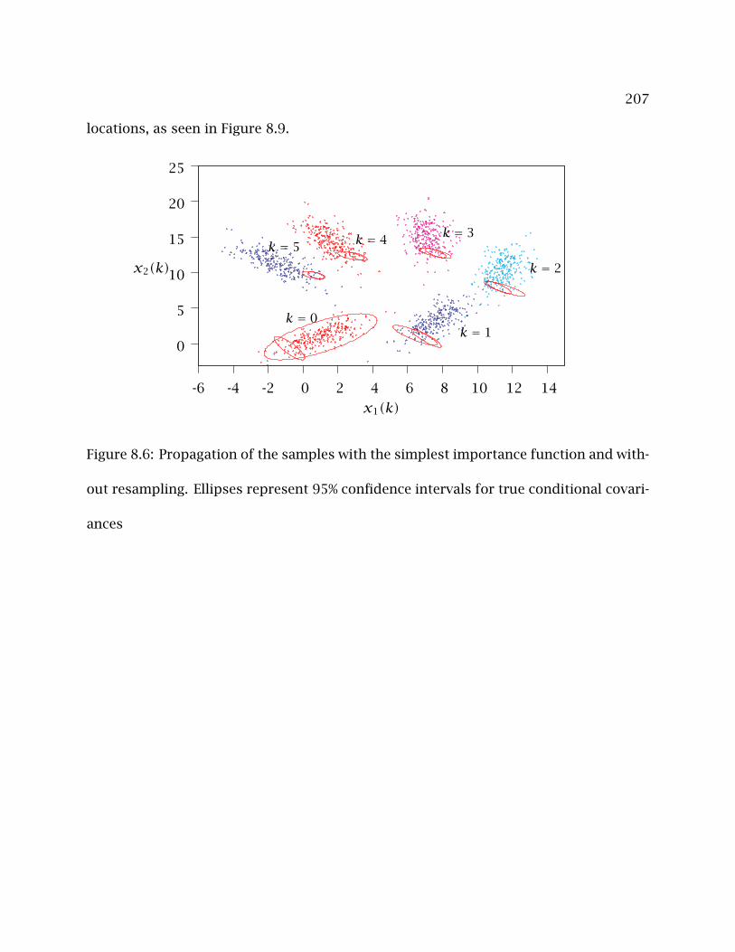
207

locations, as seen in Figure 8.9.

0

5

10

15

20

25

-6 -4 -2 0 2 4 6 8 10 12 14

x1(k)

x2(k)

k = 0k = 1

k = 2

k = 3k = 4k = 5

Figure 8.6: Propagation of the samples with the simplest importance function and with-

out resampling. Ellipses represent 95% confidence intervals for true conditional covari-

ances

208

0

5

10

15

20

-6 -4 -2 0 2 4 6 8 10 12 14

x1(k)

x2(k)

k = 0k = 1

k = 2

k = 3k = 4

k = 5

Figure 8.7: Propagation of the samples with the simplest importance function and with

resampling. Ellipses represent 95% confidence intervals for the true conditional covari-

ances

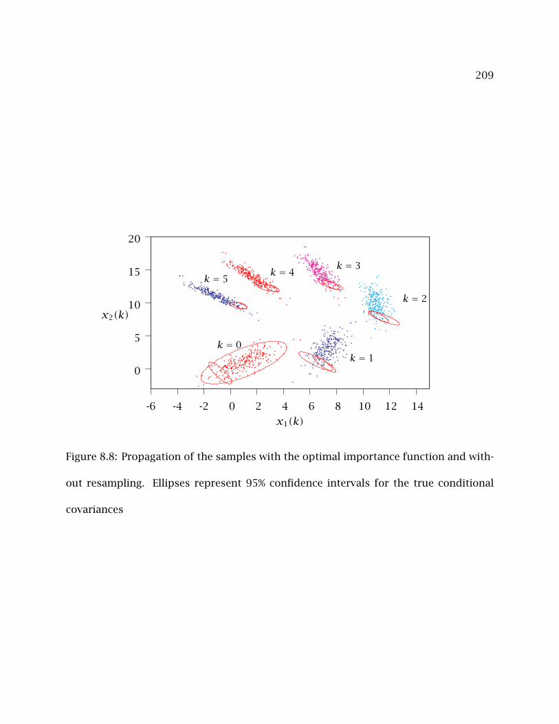
209

0

5

10

15

20

-6 -4 -2 0 2 4 6 8 10 12 14

x1(k)

x2(k)

k = 0k = 1

k = 2

k = 3k = 4

k = 5

Figure 8.8: Propagation of the samples with the optimal importance function and with-

out resampling. Ellipses represent 95% confidence intervals for the true conditional

covariances

210

0

5

10

15

20

-6 -4 -2 0 2 4 6 8 10 12 14

x1(k)

x2(k)

k = 0k = 1

k = 2

k = 3k = 4

k = 5

Figure 8.9: Propagation of the samples with the optimal importance function and with

resampling. Ellipses represent 95% confidence intervals for the true conditional covari-

ances

211

Chapter 9

Conclusions and Future Work

This dissertation contains contributions in the area of state estimation applied to model

predictive control. The techniques developed in this work are practical and can be eas-

ily included in control vendor software to improve the overall control performance.

Theoretical results developed in this work provide mathematical support to the devel-

oped techniques. Section 9.1 summarizes the major conclusions in this dissertation

and Section 9.2 presents proposals for future work in this field.

9.1 Summary of Contributions

• The Autocovariance Least-Squares (ALS) technique was developed based on au-

tocovariances in data to estimate noise statistics in the plant. The ALS technique

was shown to give smaller variance in the estimates compared to other correlation

based techniques. Simple necessary and sufficient conditions for uniqueness of

the ALS estimates were also proved.

212

• The ALS-SDP technique, that uses the trace heuristic to estimate the minimum

number of independent disturbances affecting the data, was developed.

• The optimal weighting for the ALS objective was formulated and examples were

presented to illustrate the resulting improvement in the estimates. Other practi-

cal implementation issues were presented and simplifications described to help

practitioners in coding of the ALS technique.

• The ALS technique was further developed and shown to work with misassigned

disturbance models to give offset-free model predictive control (MPC). The explicit

connections between ALS and maximum likelihood estimation techniques were

also presented.

• Simple modifications to the ALS technique were made to extend the technique to

handle nonlinear models and applications to industrial data were shown. Existing

control techniques in the industry were also shown to benefit from using the ALS

technique to specify the estimator gains.

• Finally a hybrid MHE/PF technique was presented to give good nonlinear state es-

timation. The hybrid technique uses the optimization approach in MHE to relocate

the PF samples robustly while using the PF to provide fast state estimates in be-

tween the MHE optimizations. Thus, the hybrid MHE/PF technique combines the

complimentary benefits of both the techniques.

213

9.2 Recommended Future Work

In the following sections possible directions for future work are identified.

9.2.1 Identifying Incorrect Input to Output Model

Model predictive Control (MPC) is a model based control technique and the reliability of

MPC methods is only as good as the model. Any errors in the modelling step need to be

addressed in an efficient way. For example, using a linear model for a chemical reactor

with complex dynamics would induce serious model errors if the operating point is

changed. We would require the model to be re-identified whenever the set point changes,

in order to get good control performance using MPC. There are various formulations to

quantify model errors and one such formulation is robust control, which solves a min-

max problem to calculate the optimal inputs for the worst case model error scenario.

One could argue that absorbing the model errors as a part of covariance estimation

from data would also give reasonably robust performance. The integrating disturbance

model discussed in Chapter 5 is a practical technique for accounting for model errors.

More research, however, is required to do a comparison of the integrating disturbance

model vis-a-vis other model error formulations.

A possible approach is to monitor the covariances identified using the ALS tech-

nique over time and to check the model for inconsistencies and errors, whenever large

changes in the covariance are detected. When there are no model errors the innovations

Yk is uncorrelated to the inputs uk. To detect model errors, correlations between Yk

214

and uk can be identified from data. A high correlation value signifies that the errors in

the model outputs depend on the corresponding inputs. For example, a high correlation

between Y1k and u2

k would signify that the model relation between the second input and

the first output needs to be re-identified.

9.2.2 Quantifying Closed-loop Controller Performance

MPC uses a state estimator and a controller. For the linear time-invariant case with no

constraints, the optimal state estimator is the Kalman filter and the optimal controller

is the Linear Quadratic Regulator (LQR). The separation principle (Chen, 1999) is then

applicable and the overall optimality is due to the individual optimality of the estima-

tor and the controller. For systems that are nonlinear, have constraints and/or have

model errors, the separation principle is no longer valid. The state estimator and the

controller are then coupled and any change in the estimator tuning requires the con-

troller to be re-tuned to achieve optimality. A possible future direction would be to do

a theoretical study to quantify the benefits of the control due to improved state estima-

tion. The theory of optimal control and estimation (Bryson and Ho, 1975; Anderson and

Moore, 1979) would be needed to develop the required results. This work would lend

mathematical support to the numerical results showing improvement of closed-loop

performance using the ALS technique (eg. Chapter 5 and Odelson et al. (2006a)).

215

9.2.3 Improving Nonlinear State Estimation

The results presented in Chapter 8 provide promise on application of hybrid nonlinear

estimation techniques to chemical engineering problems. The development of good

importance functions to use in particle filtering is still an active area of research. The

use of particle filtering on a trajectory of states as with moving horizon estimation is

recommended as future work. A major uncertainty is the lack of knowledge of the noise

statistics. A possible future direction is to study the effect of incorrect covariances on

the performance of sampling based and hybrid state estimation techniques.

216

217

Bibliography

A. C. Aitken. On least squares and linear combinations of observations. Proceedings of

the Royal Society of Edinburgh, 55:42–48, 1935.

B. M. Akesson, J. B. Jørgensen, N. K. Poulsen, and S. B. Jørgensen. A generalized autoco-

variance least-squares method for Kalman filter tuning. Accepted for publication in

Journal of Process Control, June 2007.

B. D. O. Anderson and J. B. Moore. Optimal Filtering. Prentice-Hall, Englewood Cliffs,

N.J., 1979.

B. D. O. Anderson and J. B. Moore. Optimal Control: Linear Quadratic Methods. Prentice-

Hall, Inc., Upper Saddle River, NJ, USA, 1990. ISBN 0-13-638560-5.

T. W. Anderson. An Introduction to Multivariate Statistical Analysis. John Wiley & Sons,

New York, third edition, 2003.

M. S. Arulampalam, S. Maskell, N. Gordon, and T. Clapp. A tutorial on particle filters

for online nonlinear/non-Gaussian Bayesian tracking. IEEE Transactions on Signal

Processing, 50(2):174–188, February 2002.

218

K. J. Astrom. Introduction to Stochastic Control Theory. Academic Press, San Diego,

California, 1970.

S. Barnett. Simplification of the lyapunov matrix equation ATPA− P = −Q. IEEE Trans-

actions on Automatic Control, 19(4):446–447, 1974.

P. Belanger. Estimation of noise covariance matrices for a linear time-varying stochastic

process. Automatica, 10:267–275, 1974.

T. Bohlin and S. F. Graebe. Issues in nonlinear stochastic grey box identification. Inter-

national Journal of Adaptive Control and Signal Processing, 9:465–490, 1995.

G. E. P. Box and G. M. Jenkins. Time Series Analysis: Forecasting and Control. Holden-Day,

San Francisco, California, 1st edition, 1970.

G. E. P. Box and G. M. Jenkins. Time Series Analysis: Forecasting and Control. Holden-Day,

Oakland, California, 1976.

G. E. P. Box and G. C. Tiao. Bayesian Inference in Statistical Analysis. Addison–Wesley,

Reading, Massachusetts, 1st edition, 1973.

G. E. P. Box, G. M. Jenkins, and G. C. Reinsel. Time Series Analysis: Forecasting and

Control. Prentice Hall, Englewood Cliffs, New Jersey, 3rd edition, 1994.

S. Boyd and L. Vandenberghe. Convex Optimization. Cambridge University Press, 2004.

S. Boyd, L. E. Ghaoui, E. Feron, and V. Balakrishnan. Linear Matrix Inequalities in Control

Theory. SIAM, Philadelphia, 1994.

219

A. E. Bryson and Y. Ho. Applied Optimal Control. Hemisphere Publishing, New York,

1975.

B. Carew and P. Belanger. Identification of optimum filter steady-state gain for systems

with unknown noise covariances. IEEE Transactions on Automatic Control, 18(6):582–

587, 1973.

C. Chen and J. Huang. Estimation of steady-state optimal filter gain from nonoptimal

Kalman filter residuals. Journal of Dynamic Systems, Measurement, and Control, 116

(3):550–553, September 1994.

C.-T. Chen. Linear System Theory and Design. Oxford University Press, 3rd edition,

1999.

C. R. Cutler and B. L. Ramaker. Dynamic matrix control—a computer control algorithm.

In Proceedings of the Joint Automatic Control Conference, 1980.

E. J. Davison and I. J. Ferguson. The design of controllers for the multivariable robust

servomechanism problem using parameter optimization methods. IEEE Transactions

on Automatic Control, 26(1):93–110, February 1981.

E. J. Davison and A. Goldenberg. Robust control of a general servomechanism problem:

the servo compensator. Automatica, 11:461–471, 1975.

E. J. Davison and H. W. Smith. Pole assignment in linear time-invariant multivariable

systems with constant disturbances. Automatica, 7:489–498, 1971.

220

J. F. G. de Freitas, M. Noranjan, A. H. Gee, and A. Doucet. Sequential Monte Carlo methods

to train neural network models. Neural Computation, 12:955–993, 2000.

D. Dee, S. Cohn, A. Dalcher, and M. Ghil. An efficient algorithm for estimating noise

covariances in distributed systems. IEEE Transactions on Automatic Control, 30(11):

1057–1065, 1985.

A. P. Dempster, N. M. Laird, and D. B. Rubin. Maximum likelihood from incomplete data

via the EM algorithm. Journal of the Royal Statistical Society: Series B, 39:1–38, 1977.

A. Doucet, S. Godsill, and C. Andrieu. On sequential Monte Carlo sampling methods for

Bayesian filtering. Statistics and Computing, 10:197–208, 2000.

D. Dougherty and D. J. Cooper. Tuning guidelines of a dynamic matrix controller for

integrating (non-self-regulating) processes. Industrial and Engineering Chemistry Re-

search, 42(8):1739–1752, 2003.

J. J. Downs. Control strategy design using model predictive control. In Proceedings of

the American Control Conference, San Diego, CA, 1999.

S. Eppler. Steady offset and integral control in model predictive control. Advanced

Independent Study, University of Wisconsin – Madison, 1997.

M. Fazel. Matrix Rank Minimization with Applications. PhD thesis, Dept. of Elec. Eng.,

Stanford University, 2002.

221

B. A. Francis and W. M. Wonham. The internal model principle for linear multivariable

regulators. J. Appl. Math. Optim., 2:170–195, 1975.

B. A. Francis and W. M. Wonham. The internal model principle of control theory. Auto-

matica, 12:457–465, 1976.

C. E. Garcıa and A. M. Morshedi. Quadratic programming solution of dynamic matrix

control (QDMC). Chemical Engineering Communications, 46:73–87, 1986.

A. Gelb, editor. Applied Optimal Estimation. The M.I.T. Press, Cambridge, Massachusetts,

1974.

A. Gelfand and A. Smith. Sampling based approaches to calculating marginal densities.

Journal of the Americal Statistical Association, 85:398–408, 1990.

M. Gevers. A personal view of the development of system identification. IEEE Control

Systems Magazine, 26(6):93–105, December 2006.

J. Geweke. Bayesian inference in econometric models using Monte Carlo integration.

Econometrica, 57(6):1317–1339, November 1989.

G. A. Ghazal and H. Neudecker. On second-order and fourth-order moments of jointly

distributed random matrices: a survey. Linear Algebra and its Applications, 321:61–

93, 2000.

G. C. Goodwin and K. S. Sin. Adaptive Filtering Prediction and Control. Prentice-Hall,

Englewood Cliffs, New Jersey, 1984.

222

A. Graham. Kronecker products and matrix calculus with applications. Ellis Horwood

Limited, West Sussex, England, 1981.

Y. Gupta. Control of integrating processes using dynamic matrix control. Chemical

Engineering Research and Design, 76(A4):465–470, May 1998.

N. B. Haaser and J. A. Sullivan. Real Analysis. Dover Publications, Inc., New York, 1991.

S. Hammarling. Numerical solution of the stable, non-negative definite lyapunov equa-

tion. IMA Journal of Numerical Analysis, 2:303–323, 1982.

E. L. Haseltine. Systems Analysis of Stochastic and Population Balance Models for Chem-

ically Reacting Systems. PhD thesis, University of Wisconsin–Madison, 2005.

E. L. Haseltine and J. B. Rawlings. Critical evaluation of extended Kalman filtering and

moving horizon estimation. Industrial and Engineering Chemistry Research, 44(8):

2451–2460, April 2005. URL http://pubs.acs.org/journals/iecred/.

J. Hedengren, K. Allsford, and J. Ramlal. Moving horizon estimation and control for an

industrial gas phase polymerization reactor. In American Control Conference, New

York, USA, July 11-13 2007.

B. Ho and R. Kalman. Efficient construction of linear state variable models from in-

put/output functions. Regelungstechnik, 14:545–548, 1966.

S. Hoang, P. De Mey, and O. Talagrand. A simple adaptive algorithm of stochastic approx-

imation type for system parameter and state estimation. In Proceedings of the 33rd

223

Conference on Decision and Control, pages 747–752, Lake Buena Vista, FL, December

1994.

S. Hoang, P. De Mey, O. Talagrand, and R. Baraille. A new reduced-order adaptive filter for

state estimation in high-dimensional systems. Automatica, 33(8):1475–1498, 1997.

D. Hua. On the symmetric solutions of linear matrix equations. Linear Algebra and its

Applications, 131:1–7, 1990.

A. Isaksson. Identification of time varying systems through adaptive Kalman filtering.

In Proceedings of the 10th IFAC World Congress, Munich, Germany, pages 305–310.

Pergamon Press, Oxford, UK, 1987.

G. Jenkins and D. Watts. Spectral Analysis and its Applications. Holden-Day, 500 Sansome

Street, San Fransisco, California, 1968.

J. Juang. Applied System Identification. Prentice Hall, Englewood Cliffs, New Jersey,

1994.

J. Juang and M. Phan. Identification of system, observer, and controller from closed-

loop experimental data. Journal of Guidance, Control, and Dynamics, 17(1):91–96,

January-February 1994.

J. Juang, C. Chen, and M. Phan. Estimation of Kalman filter gain from output residuals.

Journal of Guidance, Control, and Dynamics, 16(5):903–908, September-October 1993.

224

S. J. Julier and J. K. Uhlmann. Unscented filtering and nonlinear estimation. Proceedings

of the IEEE, 92(3):401–422, March 2004a.

S. J. Julier and J. K. Uhlmann. Corrections to unscented filtering and nonlinear estima-

tion. Proceedings of the IEEE, 92(12):1958, December 2004b.

S. J. Julier, J. K. Uhlmann, and H. F. Durrant-Whyte. A new method for the nonlinear

transformation of means and covariances in filters and estimators. IEEE Transactions

on Automatic Control, 45(3):477–482, March 2000.

R. E. Kalman and R. S. Bucy. New results in linear filtering and prediction theory. Trans.

ASME, J. Basic Engineering, pages 95–108, March 1961.

G. Kitagawa. An algorithm for solving the matrix equation X = FXFT + S. International

Journal of Control, 25(5):745–753, 1977.

A. Kong, J. S. Liu, and W. H. Wong. Sequential imputations and Bayesian missing data

problems. Journal of the Americal Statistical Association, 89(425):278–288, March

1994.

J. H. Kotecha and P. M. Djuric. Gaussian particle filtering. IEEE Transactions on Signal

Processing, 51(10):2592–2601, October 2003.

N. R. Kristensen, H. Madsen, and S. B. Jørgensen. Parameter estimation in stochastic

grey-box models. Automatica, 40:225–237, 2004a.

225

N. R. Kristensen, H. Madsen, and S. B. Jørgensen. A method for systematic improvement

of stochastic grey-box models. Computers & Chemical Engineering, 28:1431–1449,

2004b.

W. Larimore. Automated and optimal system identification by canonical variables. In

Proceedings of the American Control Conference, pages 1640–1644, Baltimore, Mary-

land, June 1994.

W. Larimore. Statistical optimality and canonical variate analysis system identification.

Signal Processing, 52(2):131–144, 1996.

J. Lee and N. Ricker. Extended Kalman filter based nonlinear model predictive control.

Industrial and Engineering Chemistry Research, 33:1530–1541, 1994.

J. H. Lee, M. Morari, and C. E. Garcıa. State-space interpretation of model predictive

control. Automatica, 30(4):707–717, 1994.

S. Li, K. Y. Lim, and D. G. Fisher. A state space formulation of model predictive control.

AIChE Journal, 35(2):241–249, February 1989.

W. Li and S. Qin. Consistent dynamic PCA based on error-in-variables subspace identi-

fication. Journal of Process Control, 11(11):661–678, 2001.

L. Ljung. System Identification: Theory for the User. Prentice-Hall, Inc., Englewood Cliffs,

New Jersey, 1987.

226

P. Lundstrom, J. H. Lee, M. Morari, and S. Skogestad. Limitations of dynamic matrix

control. Computers & Chemical Engineering, 19:409–421, 1995.

J. R. Magnus and H. Neudecker. The commutation matrix: Some properties and appli-

cations. Annals of Statistics, 7(2):381–394, March 1979.

J. R. Magnus and H. Neudecker. Matrix Differential Calculus with Applications in Statistics

and Econometrics. John Wiley, New York, 1999.

P. Marquis and J. P. Broustail. SMOC, a bridge between state space and model predictive

controllers: Application to the automation of a hydrotreating unit. In T. J. McAvoy,

Y. Arkun, and E. Zafiriou, editors, Proceedings of the 1988 IFAC Workshop on Model

Based Process Control, pages 37–43, Oxford, 1988. Pergamon Press.

J. L. Maryak, J. C. Spall, and B. D. Heydon. Use of the Kalman filter for inference in

state-space models with unknown noise distributions. IEEE Transactions on Automatic

Control, 49(1):87–90, January 2004.

R. Mehra. On the identification of variances and adaptive Kalman filtering. IEEE Trans-

actions on Automatic Control, 15(12):175–184, 1970.

R. Mehra. On-line identification of linear dynamic system with application to Kalman

filtering. IEEE Transactions on Automatic Control, 16(1):12–21, 1971.

R. Mehra. Approaches to adaptive filtering. IEEE Transactions on Automatic Control, 17:

903–908, 1972.

227

M. Morari and J. H. Lee. Model predictive control: The good, the bad, and the ugly.

In Y. Arkun and W. H. Ray, editors, Chemical Process Control—CPC IV, pages 419–

444, Amsterdam, 1991. Fourth International Conference on Chemical Process Control,

Elsevier.

M. Morari and G. Stephanopoulos. Part III: Optimal selection of secondary measurements

within the framework of state estimation in the presence of persistent unknown dis-

turbances. AIChE Journal, 26(2):247–260, 1980.

K. R. Muske and T. A. Badgwell. Disturbance modeling for offset-free linear model

predictive control. Journal of Process Control, 12(5):617–632, 2002.

K. R. Muske and J. B. Rawlings. Model predictive control with linear models. AIChE

Journal, 39(2):262–287, 1993a.

K. R. Muske and J. B. Rawlings. Linear model predictive control of unstable processes.

Journal of Process Control, 3(2):85–96, 1993b.

M. Myers and R. H. Luecke. Process control applications of an extended Kalman filter

algorithm. Computers & Chemical Engineering, 15(12):853–857, 1991.

C. Neethling and P. Young. Comments on “Identification of optimum filter steady-state

gain for systems with unknown noise covariances”. IEEE Transactions on Automatic

Control, 19(5):623–625, 1974.

J. Nocedal and S. J. Wright. Numerical Optimization. Springer-Verlag, New York, 1999.

228

G. Noriega and S. Pasupathy. Adaptive estimation of noise covariance matrices in real-

time preprocessing of geophysical data. IEEE Transactions on Geoscience and Remote

Sensing, 35(5):1146–1159, 1997.

B. J. Odelson. Estimating Disturbance Covariances From Data for Improved Control

Performance. PhD thesis, University of Wisconsin–Madison, 2003.

B. J. Odelson, A. Lutz, and J. B. Rawlings. The autocovariance least-squares methods

for estimating covariances: Application to model-based control of chemical reactors.

IEEE Control Systems Technology, 14(3):532–541, May 2006a.

B. J. Odelson, M. R. Rajamani, and J. B. Rawlings. A new autocovariance least-squares

method for estimating noise covariances. Automatica, 42(2):303–308, February

2006b. URL http://www.elsevier.com/locate/automatica.

M. Palaniswami and G. Feng. Adaptive control algorithms for disturbance rejection.

Computers and Electrical Engineering, 17(1):31–37, 1991.

G. Pannocchia. Robust offset-free model predictive control. IFAC 2002 World Congress,

Barcelona, Spain, 2002.

G. Pannocchia. Robust disturbance modeling for model predictive control with appli-

cation to multivariable ill-conditioned processes. Journal of Process Control, 13(8):

693–701, 2003.

G. Pannocchia and A. Bemporad. Combined design of disturbance model and observer

229

for offset-free model predictive control. IEEE Transactions on Automatic Control, 52

(6):1048–1053, June 2007.

G. Pannocchia and J. B. Rawlings. Disturbance models for offset-free MPC control. AIChE

Journal, 49(2):426–437, 2002.

S. J. Qin and T. A. Badgwell. A survey of industrial model predictive control technology.

Control Engineering Practice, 11(7):733–764, 2003.

S. J. Qin, W. Lin, and L. Ljung. A novel subspace identification approach with enforced

causal models. Automatica, 41(12):2043–2053, December 2005.

M. R. Rajamani and J. B. Rawlings. Estimation of noise covariances and disturbance

structure from data using least squares with optimal weighting. In Proceedings of

AIChE Annual Meeting, San Francisco, California, November 2006.

M. R. Rajamani and J. B. Rawlings. Improved state estimation using a combination of

moving horizon estimator and particle filters. In Proceedings of the American Control

Conference, New York, USA, July 11-13 2007.

M. R. Rajamani and J. B. Rawlings. Estimation of the disturbance structure from data

using semidefinite programming and optimal weighting. Accepted for publication in

Automatica, September, 2007.

M. R. Rajamani, J. B. Rawlings, S. J. Qin, and J. J. Downs. Equivalence of MPC disturbance

230

models identified from data. In Proceedings of Chemical Process Control—CPC 7, Lake

Louise, Alberta, Canada, January 2006.

M. R. Rajamani, J. B. Rawlings, and S. J. Qin. Achieving state estimation equivalence

for misassigned disturbances in offset-free model predictive control. Submitted for

publication in AIChE Journal, August, 2007.

M. R. Rajamani, J. B. Rawlings, and T. A. Soderstrom. Application of a new data-based

covariance estimation technique to a nonlinear industrial blending drum. Submitted

for publication in IEEE Transactions on Control Systems Technology, October, 2007.

C. V. Rao, J. B. Rawlings, and J. H. Lee. Constrained linear state estimation – a moving

horizon approach. Automatica, 37(10):1619–1628, 2001.

C. V. Rao, J. B. Rawlings, and D. Q. Mayne. Constrained state estimation for nonlinear

discrete-time systems: stability and moving horizon approximations. IEEE Transac-

tions on Automatic Control, 48(2):246–258, February 2003.

J. B. Rawlings and B. R. Bakshi. Particle filtering and moving horizon estimation. Com-

puters & Chemical Engineering, 30:1529–1541, 2006.

J. B. Rawlings and K. R. Muske. Stability of constrained receding horizon control. IEEE

Transactions on Automatic Control, 38(10):1512–1516, October 1993.

K. Reif, S. Gunther, E. Yaz, and R. Unbehauen. Stochastic stability of the discrete-time

231

extended Kalman filter. IEEE Transactions on Automatic Control, 44(4):714–728, April

1999.

J. Richalet, A. Rault, J. L. Testud, and J. Papon. Model predictive heuristic control: Ap-

plications to industrial processes. Automatica, 14:413–428, 1978.

D. G. Robertson, J. H. Lee, and J. B. Rawlings. A moving horizon-based approach for

least-squares state estimation. AIChE Journal, 42(8):2209–2224, August 1996.

A. Romanenko and J. A. Castro. The unscented filter as an alternative to the EKF for non-

linear state estimation: a simulation case study. Computers & Chemical Engineering,

28(3):347–355, March 15 2004.

A. Romanenko, L. O. Santos, and P. A. F. N. A. Afonso. Unscented Kalman filtering of a

simulated pH system. Industrial and Engineering Chemistry Research, 43:7531–7538,

2004.

F. C. Schweppe. Evaluation of likelihood functions for gaussian signals. IEEE Transac-

tions on Information Theory, 11(1):61–70, January 1965.

P. O. Scokaert, J. B. Rawlings, and E. S. Meadows. Discrete-time stability with perturba-

tions: Application to model predictive control. Automatica, 33(3):463–470, 1997.

F. G. Shinskey. Feedback Controllers for the Process Industries. McGraw-Hill, New York,

1994.

232

R. H. Shumway and D. S. Stoffer. An approach to time series smoothing and forecasting

using the em algorithm. Journal of Time Series Analysis, 3:253–264, 1982.

R. H. Shumway and D. S. Stoffer. Time Series Analysis and Its Applications. Springer-

Verlag, New York, 2000.

A. Sitz, U. Schwarz, and J. Kurths. The unscented Kalman filter, a powerful tool for data

analysis. 14(6):2093–2105, 2004.

A. F. M. Smith and A. E. Gelfand. Bayesian statistics without tears: A sampling-

resampling perspective. The American Statistician, 46(2):84–88, 1992.

A. G. Sparks and D. S. Bernstein. Optimal rejection of stochastic and deterministic

disturbances. Journal of Dynamic Systems, Measurement, and Control, 119:140–143,

March 1997.

W. Steeb. Kronecker product of matrices and applications. Mannheim, 1991.

D. S. Stoffer and K. Wall. Bootstrapping state space models: Gaussian maximum likeli-

hood estimation and the Kalman filter. Journal of the Americal Statistical Association,

86:1024–1033, 1991.

R. K. Sundaram. A First Course in Optimization Theory. Cambridge University Press,

1996.

M. Tenny. Computational Strategies for Nonlinear Model Predictive Control. PhD thesis,

University of Wisconsin–Madison, 2002.

233

M. J. Tenny, J. B. Rawlings, and S. J. Wright. Closed-loop behavior of nonlinear model

predictive control. AIChE Journal, 50(9):2142–2154, September 2004. URL http:

//www.aiche.org/aichejournal/.

C. F. Van Loan. The ubiquitous Kronecker product. Journal of Computational and Applied

Mathematics, 123:85–100, 2000.

P. Van Overschee and B. De Moor. N4SID: subspace algorithms for the identification of

combined deterministic-stochastic systems. Automatica, 30(1):75–93, 1994.

P. Van Overschee and B. De Moor. A unifying theorem for three subspace system iden-

tification algorithms. Automatica, 31(12):1853–1864, December 1995.

J. VanAntwerp and R. Braatz. A tutorial on linear and bilinear matrix inequalities. Journal

of Process Control, 10(4):363–385, 2000.

L. Vandenberghe and S. Boyd. A primal-dual potential reduction method for problems

involving matrix inequalities. Mathematical Programming, 69(1):205–236, 1995.

L. Vandenberghe and S. Boyd. Semidefinite programming. SIAM Review, 38(1):49–95,

March 1996.

M. Verhaegen. Identification of the deterministic part of MIMO state space models given

in innovations form from input-output data. Automatica, 30(1):61–74, 1994.

M. Viberg. Subspace methods for the identification of linear time-invariant systems.

Automatica, 31(12):1835–1851, 1995.

234

H. Wolkowicz, R. Saigal, and L. Vandenberghe, editors. Handbook of Semidefinite Pro-

gramming: Theory, Algorithms and Applications. Kluwer Academic Publishers, Mas-

sachusetts, 2000.

Y. Wu, M. Wu, D. Hu, and X. Hu. An improvement to unscented transformation. Lecture

Notes in Artificial Intelligence, 3339:1024–1029, 2004.

N. Xu and T. Shou. Optimal moving average filter with application to self-tuning type

control against deterministic disturbances. International Journal of Systems Science,

22(8):1449–1466, 1991.

W. Zhuang, M. R. Rajamani, J. B. Rawlings, and J. Stoustrup. Application of autoco-

variance least-squares method for model predictive control of hybrid ventilation in

livestock stable. In Proceedings of the American Control Conference, New York, USA,

July 11-13 2007a.

W. Zhuang, M. R. Rajamani, J. B. Rawlings, and J. Stoustrup. Model predictive control

of thermal comfort and indoor air quality in livestock stable. In Proceedings of the

European Control Conference, Kos, Greece, July 2-5 2007b.

235

Vita

Murali Rajaa Rajamani was born in Coimbatore, India on 6 June, 1980. He grew up and

lived in Mumbai, India since the age of three and finished his high school and junior

college studies from Swami Vivekanand High School/Junior College, Chembur, Mumbai

in 1998. He received his Bachelors in Chemical Engineering (B. Chem. Engg.) degree

with a gold medal from Mumbai University - Institute of Chemical Technology (formerly

University Department of Chemical Technology, Mumbai University) in 2002. In Fall

2002, he moved to Madison to brave the brutal Wisconsin winters and to start working

towards a Ph.D. degree in the Department of Chemical and Biological Engineering, Uni-

versity of Wisconsin-Madison under the supervision of Prof. James B. Rawlings. Murali

will begin work in the Advanced Control and Instrumentation group at BP Research and

Technology in Naperville, Illinois after graduation.

Permanent Address: Pune, India

This dissertation was prepared with LATEX 2ε1 by the author.

1This particular University of Wisconsin compliant style was carved from The University of Texas atAustin styles as written by Dinesh Das (LATEX 2ε), Khe–Sing The (LATEX), and John Eaton (LATEX). Knivesand chisels wielded by John Campbell and Rock Matthews.

Documents

Data-based Techniques to Improve State Estimation in Model …jbr · stay away from home for so long. My brother, Subash Rajaa, has been a constant source My brother, Subash Rajaa,