PNNL-18844

Prepared for the U.S. Department of Energy under Contract DE-AC05-76RL01830

Data Assimilation Tools for CO2 Reservoir Model Development – A Review of Key Data Types, Analyses, and Selected Software ML Rockhold GV Last EC Sullivan GD Black CJ Murray PD Thorne September 2009

DISCLAIMER This report was prepared as an account of work sponsored by an agency of the United States Government. Neither the United States Government nor any agency thereof, nor Battelle Memorial Institute, nor any of their employees, makes any warranty, express or implied, or assumes any legal liability or responsibility for the accuracy, completeness, or usefulness of any information, apparatus, product, or process disclosed, or represents that its use would not infringe privately owned rights. Reference herein to any specific commercial product, process, or service by trade name, trademark, manufacturer, or otherwise does not necessarily constitute or imply its endorsement, recommendation, or favoring by the United States Government or any agency thereof, or Battelle Memorial Institute. The views and opinions of authors expressed herein do not necessarily state or reflect those of the United States Government or any agency thereof.

PACIFIC NORTHWEST NATIONAL LABORATORY operated by BATTELLE

for the UNITED STATES DEPARTMENT OF ENERGY

under Contract DE-AC05-76RL01830

Printed in the United States of America

Available to DOE and DOE contractors from the Office of Scientific and Technical Information,

P.O. Box 62, Oak Ridge, TN 37831-0062; ph: (865) 576-8401 fax: (865) 576-5728 email: reports@adonis.osti.gov

Available to the public from the National Technical Information Service, U.S. Department of Commerce, 5285 Port Royal Rd., Springfield, VA 22161 ph:

(800) 553-6847 fax: (703) 605-6900 email: orders@ntis.fedworld.gov online ordering: http://www.ntis.gov/ordering.htm

This document was printed on recycled paper. (9/2003)

PNNL-18844

Data Assimilation Tools for CO2 Reservoir Model Development – A Review of Key Data Types, Analyses, and Selected Software

ML Rockhold GV Last EC Sullivan GD Black CJ Murray PD Thorne

September 2009 Prepared for the U.S. Department of Energy under Contract DE-AC05-76RL01830 Pacific Northwest National Laboratory Richland, Washington 99352

iii

Abstract

Pacific Northwest National Laboratory (PNNL) has embarked on an initiative to develop world-class capabilities for performing experimental and computational analyses associated with geologic sequestration of carbon dioxide. The ultimate goal of this initiative is to provide science-based solutions for helping to mitigate the adverse effects of greenhouse gas emissions. This Laboratory-Directed Research and Development (LDRD) initiative currently has two primary focus areas—advanced experimental methods and computational analysis. The experimental methods focus area involves the development of new experimental capabilities, supported in part by the U.S. Department of Energy’s (DOE) Environmental Molecular Science Laboratory (EMSL) housed at PNNL, for quantifying mineral reaction kinetics with CO2 under high temperature and pressure (supercritical) conditions. The computational analysis focus area involves numerical simulation of coupled, multi-scale processes associated with CO2 sequestration in geologic media, and the development of software to facilitate building and parameterizing conceptual and numerical models of subsurface reservoirs that represent geologic repositories for injected CO2. This report describes work in support of the computational analysis focus area.

The computational analysis focus area currently consists of several collaborative research projects. These are all focused on the development and application of conceptual and numerical models for geologic sequestration of CO2. The software being developed for this focus area is referred to as the Geologic Sequestration Software Suite or GS3. A wiki-based software framework is being developed to support GS3. This report summarizes work performed in FY09 on one of the LDRD projects in the computational analysis focus area. The title of this project is Data Assimilation Tools for CO2 Reservoir Model Development. Some key objectives of this project in FY09 were to assess the current state-of-the-art in reservoir model development, the data types and analyses that need to be performed in order to develop and parameterize credible and robust reservoir simulation models, and to review existing software that is applicable to these analyses. This report describes this effort and highlights areas in which additional software development, wiki application extensions, or related GS3 infrastructure development may be warranted.

v

vii

Acknowledgments

The authors would like to acknowledge the support of two student interns—Colleen Devoto and Ellery Newcomer. Colleen is a junior at the University of Texas – San Antonio, majoring in Geology. Colleen contributed to compiling reference information and physicochemical property data for populating a Rock Properties Catalog that will eventually be accessible from the GS3 wiki. Ellery is a senior at the University of Tulsa, majoring in Computer Science. Ellery contributed to the testing and evaluation of selected software packages, and to the development of some well log analysis tools that are demonstrated in this report. We would also like to thank Mike Fayer and Terri Stewart for providing support for two of the authors (Rockhold and Sullivan) to attend a Schlumberger Petrel training course in Houston, Texas.

ix

Acronyms and Abbreviations

DOE U.S. Department of Energy EMSL Environmental Molecular Science Laboratory LDRD Laboratory-Directed Research and Development PNNL Pacific Northwest National Laboratory

xi

Contents

Abstract ........................................................................................................................................................ iii Acknowledgments.......................................................................................................................................vii Acronyms and Abbreviations ...................................................................................................................... ix 1.0  Introduction ....................................................................................................................................... 1.1 2.0  Overview of Conceptual Model Development and Its Role in Subsurface Carbon

Sequestration ..................................................................................................................................... 2.1 2.1  Definition of Conceptual Models .............................................................................................. 2.1 2.2  Need for Conceptual Models..................................................................................................... 2.2 2.3  Approach to Data Assimilation and Development of Conceptual Models ............................... 2.3 

3.0  Reservoir Characterization ................................................................................................................ 3.1 3.1  Overview ................................................................................................................................... 3.1 

4.0  Recommendations for Enhancing PNNL Model Building Capabilities and GS3 Software .............. 4.1 5.0  Summary and Conclusions ................................................................................................................ 5.1 6.0  References ......................................................................................................................................... 6.1 Appendix A Reservoir Characterization Data Types and Analyses ......................................................... A.1 Appendix B Review of Selected Software.................................................................................................B.1 

xii

Figures

Figure 1.1. Geological Sequestration Software Suite (GS3) Modeling Workflow ................................... 1.2 Figure 1.2. The GS3 Software Architecture .............................................................................................. 1.3 Figure A.1. Example of Core Log............................................................................................................ A.4 Figure A.2. Exposure of the Tensleep Sandstone and Opeche Cap Rock (Milliken and Black,

2007) ................................................................................................................................................. A.5 Figure A.3. Comparison of Outcrops of Cretaceous Rudist Reefs in Texas with Very Similar

Lithofacies Seen In a Resistivity-Based Image Log from a Deep Hydrocarbon Exploration Well (Sullivan 2005)........................................................................................................................ A.6 

Figure A.4. Left: Outcrop Contact between a Massive Basalt Flow and the Weathered Flow Top of the Underlying Basalt Flow near Dayton, Washington. Right: Sonic Log Signature of the Same Type of Lithofacies from the Big Sky Basalt Sequestration Pilot Well Near Wallula, Washington ....................................................................................................................................... A.6 

Figure A.5. Example of Whole Core from the Tensleep Fm at the Teapot Dome Field (Well 48-X-28), Slabbed and Photographed using Natural and Ultraviolet Light........................................... A.7 

Figure A.6. Portable Gamma-Ray Logging of Core ................................................................................ A.8 Figure A.7. Tensleep Core Sub-sampled for Laboratory Analyses ......................................................... A.8 Figure A.8. Rotary Sidewall Cores from the Big Sky Basalt Carbon Sequestration Pilot at

Wallula, Washington ........................................................................................................................ A.9 Figure A.9. Photomicrograph of Tensleep Sandstone (5,498’ Sample) in Plane Light at 200 x

Magnification Showing Some Moldic Dissolution Voids (Blue) That Have Been Partially Filled by Dolomite. Minor Amounts of Siderite (Brown Material) are Also Present (Coughlin 1982).............................................................................................................................. A.10 

Figure A.10. Physical Analyses of Core Samples.................................................................................. A.11 Figure A.11. Example of Permeability and Fluid Saturation versus Porosity Cross Plots .................... A.11 Figure A.12. Relative Permeability of the Oil and Water (Simulated Brine) Phases Relative to

that of the Air (Gas) Phase in a Tensleep Core Sample at a Confining Stress of 3000 psi (Hurley, 1986)................................................................................................................................. A.12 

Figure A.13. Crossplot of In Situ Archie Cementation Exponent (m) versus In Situ Porosity for Various Lithofacies in the Hugoton Gas Field (Dubois et al. 2006)............................................... A.13 

Figure A.14. Segment of a resistivity based image log showing textures in a carbonate reservoir. Tadpoles and rose diagram represent stratigraphic dip and dip azimuth (Sullivan 2005) .............. A.18 

Figure A.15. Segment of Resistivity Based Image Log from the 2009 Big Sky Basalt Sequestration Pilot well in Wallula, Washington ........................................................................... A.19 

Figure A.16. Time lapse pulsed neutron sigma logs from the 2004 Frio sequestration experiment, near Houston Texas. The computed lithofacies are shown to the left, and to the right are the changes of CO2 saturations near the wellbore with time, as measured by logging runs through November 2, 2004. ............................................................................................................ A.22 

Figure A.17. Wiggle trace display of a line of seismic data, overlaid with a synthetic seismogram generated from a sonic log and density log. (Shown in two-way travel time) (SEPM Sequence Stratigraphy Web 2009).................................................................................................. A.24 

Figure A.18. Mechanical properties of the Wallula Basalt Sequestration pilot, as measured by Schlumberger's advanced sonic tool, the Sonic Scanner. The Platform Express suite of logs

xiii

on the left shows position of porous basalt flow tops (2410-2440) and massive flow interiors (2580-2650) that are potential seals (Martinez 2009). .................................................................... A.25 

Figure A.19. Comparison of Stoneley Wave Porosity with Computer Generated ELAN (Elemental Analysis) Composite Log. Data from the 2009 Big Sky Basalt Sequestration Well (Martinez 2009)...................................................................................................................... A.26 

Figure A.20. Depiction of NML Signal and Estimation of “Free Fluid” Porosity, φf............................ A.29 Figure A.21. UMAA Versus RHOMMA Crossplot Showing Values for Some Common Minerals

from Table 3.4 and Computed Log Data from Well 48-X-28 at the Teapot Dome Field, Wyoming ........................................................................................................................................ A.32 

Figure A.22. Measured Gamma Ray (GR), Neutron-Porosity (NPOR) Logs, Computed Apparent Matrix Density (RHOMAA), Apparent Matrix Volumetric Cross Section (UMAA), and Mineral Volume Fraction Logs for the Tensleep Sandstone Formation in Well 48-X-28 at the Teapot Dome Field, Powder River Basin, Wyoming. The horizontal lines on the UMAA log plot represent the unit tops reported for this well by Rocky Mountain Oilfield Testing Center, Casper, Wyoming............................................................................................................... A.33 

Figure A.23. Example of Depth Registered Geologic Picks or Formation Tops and Geologists Comments (These are an Important Component of Reservoir Models) (McGrail et al. 2006d) .... A.36 

Figure A.24. P-Wave Seismic Source Trucks, Part of the 3C Seismic Program In Support of the Basalt Carbon Sequestration Pilot Test at Wallula Washington. Each of These Trucks Has a Vibrating Metal Plate That Can Generate 64,000 Pounds of Earth Force. ..................................... A.38 

Figure A.25. Wiggle-Trace Display of P-Wave 2D Seismic Data from the Recently Re-started Futuregen Sequestration Project at Mattoon, Illinois. Dark Events Represent Velocity Contrasts Associated With Changes in Rock, Fluid, Pressure, or Geomechanical Properties. ...... A.39 

Figure A.26. Converted Wave P-S Seismic Data; Mattoon 2D Seismic Line 2. These Less Distinct-Looking Data Have High Information Content, but Image Different Geological Properties Compared to P Wave Data. Assimilation of Converted Wave Data Represents a New Research Opportunity for Modeling Sequestration Reservoirs. ............................................. A.40 

Figure A.27. Source and Receiver Geometry used in the Four-Mile Long, 3C Data-Acquisition Swath Acquired for the Wallula Basalt Sequestration Pilot. Source Stations Represent GPS Located Positions Occupied by Vibroseis Trucks. ......................................................................... A.41 

Figure A.28. P-Wave Cross-Section Image of the Geology Along One of the 2D Seismic Lines Acquired by PNNL in Support of the Proposed Mattoon Futuregen Sequestration Site. The Top of the Mount Simon Sandstone Sequestration Target is Shown in Magenta. Seismic Line is About Six Miles Long. Red Line is the Projected Location of a Possible Characterization Well (Leetaru 2009). ........................................................................................... A.44 

Figure A.29. Interpreted Structure Map (In Depth below Ground Surface) on Top of the Mount Simon Reservoir at the Proposed Mattoon Futuregen Site. Location of the 2D Seismic Lines from Which the Data were Interpreted, Depth Converted, and Subsequently Mapped are Shown as Lines of Small Dots. The Longest Seismic Line is About Seven Miles (Leetaru 2009). .............................................................................................................................................. A.45 

Figure A.30. Overlay of One Line of the Original 3D Seismic Data and Sonic Well Curves on the Impedance Inversion of Seismic Data from an Oil Field in West Texas. Original Seismic Traces and Well Logs are in Black; Colored Data are the Inverted Volume, Which Shows Considerably More Detail. Blue Oval Outlines a Channel-Like Feature. Impedance is in Km/Sec* Gm/Cc (Fu et al. 2006). .................................................................................................. A.47 

Figure A.31. Map View of Unsupervised Facies Classification Output. Black Shapes are Faults; Sinuous Blue Feature is a Channel (James 2009). .......................................................................... A.48 

xiv

Figure A.32. Curvature in Two Dimensions. Curvature is Defined as the Inverse of the Radius of a Circle that is Tangent to a Surface at any Point. By Convention, Positive Curvature is Convex Upward; Negative Curvature is Convex Downward. Anticlines Have Positive Curvature; Synclines Have Negative Curvature (Blumentritt et al. 2006). .................................... A.49 

Figure A.33. Map-View Time Slice through a Fort Worth Basin 3D Mean Curvature Seismic Attribute Volume at 1.18 S., Near the Top of the Ordovician Ellenburger Formation. Note the Crisp Imaging of the Subcircular Sinkhole Collapse Features. Scale Bar is Five Kilometers. (Sullivan et al. 2005) .................................................................................................. A.49 

Figure A.34. Time Slice from a Multi-Attribute Volume Generated from the Same Fort Worth Basin 3-D Survey as Viewed in Figure A.33.................................................................................. A.50 

Figure A.35. Comparison of Lineaments Mapped From Positive and Negative Curvature Attributes ........................................................................................................................................ A.50 

Figure A.36. Most Negative Curvature Seismic Attribute along a Stratal Surface within Mississippian Carbonates in a Depleted Kansas Reservoir ............................................................ A.51 

Figure A.37. Maps of P and P-S Amplitude-based Seismic Facies (top) from a Hydrocarbon Field in the Permian Basin of West Texas Showing Distribution of Seismic Facies that Coincide with Porous and Permeable Reservoir Rock. Vertical Sections through P and P-S Data Volumes along Inline 67 (bottom) that Traverses the Center of the Maps. Solid Circles = Hydrocarbon Producers; Open Circles = Nonproducers. (Hardage et al. 2008) ........................ A.53 

Figure A.38. Comparisons of P (left) and P-S (right) Reflectivities across (a) a High-Saturation Gas Reservoir and (b) a Low-Saturation Natural Gas Reservoir. Rectangular Windows are Centered on the Reservoirs. Converted Wave P-S Images Distinguish These Two; P-wave Images Do Not. (Hardage 2009).................................................................................................... A.54 

Figure A.39. Generalized Workflow for Integrating Seismic Attributes into Characterization of Fractured Reservoirs. The Resulting Insights and Information Provide Input for Reservoir Geomodels. (Sullivan et al. 2006).................................................................................................. A.56 

Figure A.40. Relation of Fracture Orientation to Principle Earth Stress Tensors.................................. A.59 Figure A.41. Schematic Map View Looking Down On a Wellbore Showing Ellipse Formed By

Breakage of Rock Aligned With Regional Earth Stress in the Borehole........................................ A.59 Figure A.42. Location of 2006 Proposed West Texas FutureGen Site with Proposed Injection

Wells and Map-View Projection of Faults Below the Guadalupian Sandstone Injection Zone. Fractures May or May Not Extend From the Deep Subsurface into the Reservoir Zone. Fractures Striking Parallel to Maximum Horizontal Stress Might be at Greater Risk of Opening During Injection. (McGrail et al. 2006d) ........................................................................ A.60 

Figure A.43. Seismic-based Schematic Drawing of Tectonic Setting of 2006 Proposed West Texas FutureGen Site...................................................................................................................... A.61 

Figure A.44. Map View (right) of Microseismic Fracture-Opening Patterns Formed During a Large Subsurface Hydrofracture Stimulation of a Well in the Fort Worth Basin of North Texas (Simon 2005)........................................................................................................................ A.62 

Figure A.45. Localized Changes in Stress Orientation in Four Wells along a Polyphase Fault in West Texas (Sullivan et al. 2005) ................................................................................................... A.63 

Figure A.46. Cutaway View of Geologic Units for a Portion of the Teapot Dome Field in Wyoming, Generated Using EarthVision™ ................................................................................... A.67 

Figure A.47. Cross-Section Schematic Drawing of Transgression and Regression of a Marine Shoreline. The Response to Rising and Falling Sea Level Produces Offsetting Stratal

xv

Geometries that are Seismic Scale and that are the Basis for Defining the Architecture of Sedimentary Reservoir Models. (SEPM Sequence Stratigraphy Web 2009) ................................ A.69 

Figure A.48. Outcrop-based, Permian Sequence Stratigraphic Model of the Northwest Margin of the Delaware Basin. The Reservoirs of the 2006 Proposed West Texas FutureGen Sequestration Field, on the Southeast Side of the Delaware Basin, were in the Lowstand Brushy Canyon Sandstones. (Beaubouef et al. 1999).................................................................... A.70 

Figure A.49. East-West Seismic Line across the Permian Shelf Margin of the Central Basin Platform in West Texas, Including the Subsurface Equivalents of the Lower Guadalupian Strata Shown in the Previous Figure. The Recognition Of These Same Outcrop–Based sequence Stratigraphic Relationships in the Subsurface Forms a Powerful Predictive Tool for Reservoir Continuity and Performance. (Dou et al. 2009) ............................................................ A.70 

Figure A.50. Outcrops of the Delaware Basin Sandstones Correlative to the Reservoirs in the 2006 Proposed West Texas FutureGen Site. The Permian Reefal Carbonates (White Cliffs) that Prograded Over Slope and Basinal Sandstones (Dark) are Visible in the Background. (Sullivan 2000) ............................................................................................................................... A.71 

Figure A.51. Outcrop-based Sequence Stratigraphic Analysis of Cretaceous Carbonate Reservoir Analogs in Texas. Here Cycles (High Frequency Cycles) are Grouped into High Frequency Cycle Sets (Parasequences) Which are in Turn Grouped into Large Packages (Facies Tracts) that Reflect Base Level or Sea Level Changes. (Kerans 2002) ..................................................... A.72 

Figure A.52. Stacking of Lithofacies to Form Parasequences. Prograding (Seaward Advancing) Parasequences as Interpreted from Outcrops in the Book Cliffs of Wyoming. (SEPM Sequence Stratigraphy Web 2009).................................................................................................. A.73 

Figure A.53. Example of Steep Prograding Shelf Margin in the Subsurface of the Northern Delaware Basin of New Mexico ..................................................................................................... A.74 

Figure A.54. Section of a 1D Geostatistical Facies Model for Wallula Basalts Over a 2000 Foot Well Interval. Summary of Image Log Interpreted Bed Dips are on the Right, and are Plotted Against the Facies Colors on the Left. The Program Interprets Dip Reversal as Faults; Examination of the Data Indicates Dip Reversals are Stratigraphic. .................................. A.76 

Figure A.55. Examples of Experimental and Fitted Model Variograms ............................................... A.79 Figure A.56. Illustration of the Sequential Simulation Algorithm......................................................... A.81 Figure A.57. Diagram Showing the 16 Possible Patterns of Distribution of 2 Lithofacies for a

Four-Cell Scanning Template (Boisvert et al. 2008) ...................................................................... A.83 Figure A.58. Illustrations of 2 Facies Categorical Realizations Generated using Multiple-Point

Geostatistics (A) and Indicator Geostatistics (B) (Strebelle 2002)................................................. A.84 

xvi

Tables

Table A.1. X-Ray Diffraction Analysis of Whole Rock and <5 Micrometer Size Fraction of Two Samples of the Tensleep "Zone A" Sandstone (Coughlin 1982) ...................................................... A.8 

Table A.2. Petrophysical and Mechanical Rock Properties (Hecht et al. 2005) .................................... A.14 Table A.3. Dielectric Permittivity (a.k.a. Dielectric Constant) Relative to Air and Propagation

Times For Some Common Reservoir Rocks, Minerals, and Fluids (Schlumberger 1989)............. A.28 Table A.4. Photoelectric cross section, specific gravity, log density, and volumetric cross section

index for some common minerals and fluids (Schlumberger 1989, Ellis and Singer 2007)........... A.31 

1.1

1.0 Introduction

Subsurface reservoir characterization and model development are typically associated with the petroleum exploration and production industry for which the resource of primary interest is hydrocarbons—both oil and gas. As our known oil and gas reserves become depleted, renewed emphasis has been placed on other fossil fuels including coal and oil shale. Both of these energy sources are somewhat problematic. Burning of coal is “dirty” relative to oil and gas combustion, and oil shale is notoriously difficult to extract economically. Regardless of the fossil fuel, subsurface characterization must be performed and reservoir models must be developed to evaluate the extent of the resources and the viability or economics of their extraction.

Associated with the world’s current over-reliance on fossil fuels is the generation of greenhouse gases, including CO2. One of several potential methods for mitigating the excessive production of CO2 is to inject it into the subsurface – a process known as geologic sequestration. Since CO2 is not, as of yet, considered to be a valuable commodity, current economics dictate that geologic sequestration would be most viable if the injection sites are located nearby existing power plants where the CO2 is being produced, to minimize transportation costs. Determining the suitability of any particular site for subsurface injection and sequestration of CO2 also requires characterization data and development of reservoir models that can be used to predict the long-term performance of the reservoir and its cap rock for retaining or transforming the CO2 such that it remains effectively sequestered in the subsurface rather than being released into the atmosphere. The U.S. Environmental Protection Agency has recently developed Federal Requirements on underground injection control (UIC) for wells used specifically for geologic sequestration of CO2 (40 CFR Parts 144 and 146 ).

Pacific Northwest National Laboratory (PNNL) has embarked on an initiative to develop world-class capabilities for performing experimental and computational analyses associated with geologic sequestration of carbon dioxide. This Laboratory-Directed Research and Development (LDRD) initiative currently has two primary focus areas – experimental and computational. The experimental focus area involves the development of new experimental capabilities, supported in part by the U.S. Department of Energy’s Environmental Molecular Science Laboratory (EMSL) housed at PNNL, for quantifying mineral reaction kinetics with CO2 under high temperature and pressure (a.k.a. supercritical) conditions. The computational focus area involves numerical simulation of coupled, multi-scale processes associated with CO2 sequestration in geologic media, and the development of software to facilitate building and parameterizing conceptual and numerical models of subsurface reservoirs that represent geologic repositories for injected CO2.

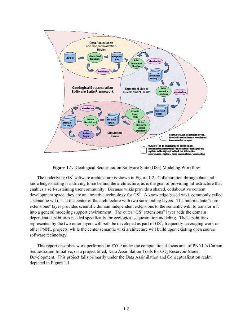
The software and the associated applications framework for the computational focus area are collectively referred to as the Geologic Sequestration Software Suite or GS3. A wiki-based software framework is being developed to support GS3. Figure 1.1 depicts the workflow for geological sequestration modeling that will be supported by the GS3 framework, broken into three general realms—Data Assimilation and Conceptualization, Numerical Model Development, and Simulation. The feedback loops throughout the workflow will allow users to iteratively refine the models they are developing. Although not depicted in the figure, the user will also be able to re-enter the workflow at arbitrary points in order to explore different “what if…” scenarios.

1.2

Figure 1.1. Geological Sequestration Software Suite (GS3) Modeling Workflow

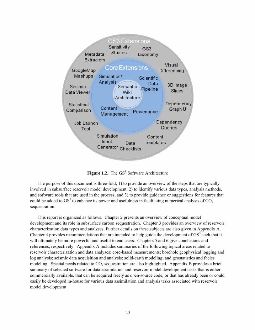
The underlying GS3 software architecture is shown in Figure 1.2. Collaboration through data and knowledge sharing is a driving force behind the architecture, as is the goal of providing infrastructure that enables a self-sustaining user community. Because wikis provide a shared, collaborative content development space, they are an attractive technology for GS3. A knowledge based wiki, commonly called a semantic wiki, is at the center of the architecture with two surrounding layers. The intermediate “core extensions” layer provides scientific domain independent extensions to the semantic wiki to transform it into a general modeling support environment. The outer “GS3 extensions” layer adds the domain dependent capabilities needed specifically for geological sequestration modeling. The capabilities represented by the two outer layers will both be developed as part of GS3, frequently leveraging work on other PNNL projects, while the center semantic wiki architecture will build upon existing open source software technology.

This report describes work performed in FY09 under the computational focus area of PNNL’s Carbon Sequestration Initiative, on a project titled, Data Assimilation Tools for CO2 Reservoir Model Development. This project falls primarily under the Data Assimilation and Conceptualization realm depicted in Figure 1.1.

1.3

Figure 1.2. The GS3 Software Architecture

The purpose of this document is three-fold; 1) to provide an overview of the steps that are typically involved in subsurface reservoir model development, 2) to identify various data types, analysis methods, and software tools that are used in the process, and 3) to provide guidance or suggestions for features that could be added to GS3 to enhance its power and usefulness in facilitating numerical analysis of CO2 sequestration.

This report is organized as follows. Chapter 2 presents an overview of conceptual model development and its role in subsurface carbon sequestration. Chapter 3 provides an overview of reservoir characterization data types and analyses. Further details on these subjects are also given in Appendix A. Chapter 4 provides recommendations that are intended to help guide the development of GS3 such that it will ultimately be more powerful and useful to end users. Chapters 5 and 6 give conclusions and references, respectively. Appendix A includes summaries of the following topical areas related to reservoir characterization and data analyses: core-based measurements; borehole geophysical logging and log analysis; seismic data acquisition and analysis; solid-earth modeling; and geostatistics and facies modeling. Special needs related to CO2 sequestration are also highlighted. Appendix B provides a brief summary of selected software for data assimilation and reservoir model development tasks that is either commercially available, that can be acquired freely as open-source code, or that has already been or could easily be developed in-house for various data assimilation and analysis tasks associated with reservoir model development.

2.1

2.0 Overview of Conceptual Model Development and Its Role in Subsurface Carbon Sequestration

Modeling of the injection and reactive transport of CO2 plays a central role in decision-making in subsurface carbon sequestration, including evaluation of potential sequestration sites, injection well location, design of injection wells and supporting infrastructure, and design of monitoring, mitigation, and validation plans. A major step in the modeling process is development of one or more conceptual models of a site and the data assimilation needed in that development.

A first step in the modeling process is identification of the type and purpose of modeling that are needed (Anderson and Woessner 1992, Neuman and Wierenga 2003). Anderson and Woessner (1992) identify three major types of modeling: predictive, interpretive, and generic. Most modeling that would be performed for subsurface CO2 sequestration would be predictive in nature, intended to predict the outcome of some future action related to sequestration. The purpose of modeling will vary considerably based on the state of a site. At one end of the spectrum, this would include simple scoping models generated using data from analogous sites that might be used for a preliminary estimation of the storage capacity and injectivity of a proposed sequestration site; in that case, there would be little to no characterization data available from a site. At the other end of the spectrum would be the evaluation of an existing monitoring, mitigation, and validation plan for a site after several years of injection. Revision of an existing conceptual model in this case would usually involve integration and assimilation of large amounts of many types of data, including core data, geophysical well logs, 3- and/or 4-dimensional seismic data, CO2 injection and pressure data, and concentration data from existing monitoring wells.

The remainder of this section will define conceptual models, provide motivation for their development, including associated data assimilation, and identify an approach to the development of conceptual models that will serve as an introduction to the data types and analyses needed to support their development.

2.1 Definition of Conceptual Models

Anderson and Woessner (1992) define a conceptual model as a pictorial diagram that represents the major geologic elements present in the flow system, and is often developed as a block diagram or a geologic cross-section. The elements and scale of the conceptual model constrain the dimensions of the numerical model and associated grids. The construction of the conceptual model fulfills two main goals, the simplification of the field problem and the organization of data available from the field area. Simplification is necessary because it is not possible to capture all of the complexity of the field problem in a numerical model. Anderson and Woessner (1992) discuss the concept of model parsimony, that the model be as simple as possible, while still retaining sufficient complexity that the model reproduces known system behavior.

A National Research Council study of conceptual models (NRC 2001) defined them as “an evolving hypothesis identifying the important features, processes, and events controlling fluid flow and contaminant transport of consequence at a specific field site in the context of a recognized problem.” This definition emphasizes that the conceptual model evolves as new data becomes available, and must be tested to ensure it is internally consistent and that numerical simulations of flow and transport based on it

2.2

are able to reproduce system behavior. Like Anderson and Woessner, they state that while conceptual models represent simplifications of reality, they must retain enough complexity to allow the problem under review to be reasonably addressed.

2.2 Need for Conceptual Models

One of the major aspects of carbon sequestration modeling that drives the need for development of conceptual models is the requirement for decision making under uncertainty. Possible uses of numerical modeling for decision making in carbon sequestration would include (among others) estimation of the volume available for storage of CO2, the rate at which CO2 could be injected, the placement and design of injection wells, the potential impact of geological heterogeneity on capacity and injectivity, and the design of monitoring networks for sequestration sites. For example, Ambrose et al. (2008) discuss the impact of structural heterogeneity (faults, folds, and fracture intensity) and stratigraphic heterogeneity (principally the geometry of depositional facies and the continuity of sand bodies) on CO2 storage capacity and retention using examples from Gulf Coast oil and gas reservoirs. Chadwick et al. (2004) discuss the impact of stratigraphic and structural permeability barriers within Sleipner field in the North Sea on the migration of CO2 within the aquifer; those barriers were difficult to predict prior to the start of injection and led to unexpected migration paths for the injected CO2.

The prediction needs outlined above are very similar to the requirements of predictions for environmental studies in hydrogeology (e.g., Neuman and Wierenga 2003) and petroleum reservoir modeling (Deutsch 2002). As those authors point out, there will always be uncertainty in our representation of subsurface properties. Much of this uncertainty arises because of our inability to completely sample the subsurface, with just a few wells providing direct measurements of required properties for large volumes of the subsurface and even seismic data are often on a relatively coarse grid (for example, see Chadwick et al. 2004). This spatial uncertainty is compounded by the effects of geological heterogeneity, which leads to significant local variations in subsurface properties that will impact carbon sequestration. In addition, uncertainty in predictions also arises due to uncertainty in the measurements that are used for subsurface characterization. This can be due to both inherent instrumental variability, but also in many cases, we end up with measurements of properties that are not those we’re looking for, but properties that are correlated with them.

Because of these uncertainties, Neuman and Wierenga (2003), Deutsch (2002), and other authors recommend the use of a stochastic or probabilistic approach to the characterization of aquifers and reservoirs. This might include the use of Monte Carlo approaches to capture the variability in site parameters, together with geostatistical realizations (i.e., stochastic simulations) that provide multiple alternative realizations of the site properties (Deutsch 2002). Each of the multiple realizations, or some subset of them, can then be evaluated through the numerical flow simulator, providing a suite of predictions of important system properties. This would provide both an estimate of the most likely outcome as well as an assessment of the uncertainty associated with that estimate. A suite of stochastic realizations could also be used for specific evaluation of proposed plans for an injection site. For example, a suite of stochastic realizations could be input to a CO2 flow and transport model to evaluate the probability that a proposed monitoring network design would be successful in capturing the characteristics of an injected plume of CO2; this might be quantified as the percentage of realizations in which the proposed monitoring network intercepts a given percentage of the plume volume.

2.3

One important characteristic of the probabilistic approach described above is the use of multiple conceptual models. Each conceptual model could represent an alternative hypothesis about the important geologic and hydrologic features of the site, in line with the definition of a conceptual model proposed by the National Research Council (NRC 2001) and discussed above. For example, Neuman and Wierenga (2003) suggest a large number of properties of the conceptual model that might be candidates for development of alternative conceptual models, including the resolution of the model in space and time; the number and distribution of hydrogeologic layers; the spatial configuration of structures such as faults; and the spatial distribution of properties like porosity and hydraulic conductivity. The use of alternative conceptual models allows for an assessment of the uncertainty in site predictions resulting from the various alternative models. By comparing predictions generated using the alternative conceptual models with monitoring data, it is possible to evaluate and rank the conceptual models (Neuman and Wierenga 2003, Meyer et al. 2007). Note that without some form of monitoring data, it is only possible to rank conceptual models based on their consistency with available site characterization data (Neuman and Wierenga 2003).

2.3 Approach to Data Assimilation and Development of Conceptual Models

Several steps are important in the development of conceptual models, and the data assimilation that is required in their development. The first step is definition of the question to be addressed by the numerical models that will be generated from the conceptual model (Anderson and Woessner 1992). In the context of carbon sequestration, the identification of the questions to be addressed by the numerical model provides a significant constraint on the modeling process. For example, a simple one dimensional model that is radially symmetric may be all that is needed for an initial scoping examination of a site to determine if it should have sufficient storage capacity and injectivity to be a good candidate for carbon sequestration. The level of detail needed for a model used to evaluate the performance of a monitoring network after several years of CO2 injection would be significantly higher.

The amount of available data will also play into the complexity of the numerical model, and will usually be related to the questions that need to be addressed by the numerical modeling effort. In the first example given above, there might be little to no data available from the site, and most of the data analysis may be based on data from analogous reservoirs located a considerable distance away. The data management and analysis needs for evaluation of an existing sequestration project, or for a carbon sequestration project planned for a well-characterized depleted oil and gas reservoir, will be much greater.

After definition of the questions to be addressed by the modeling and preliminary identification of the amount and types of data that will be available for definition of the conceptual model it is necessary to assemble and organize the available data. Neuman and Wierenga (2003) provide a detailed description of the needs for assembly of the hydrogeologic knowledge base required for numerical modeling of nuclear facilities and sites. While the regulatory needs for carbon sequestration are not as stringent as those for siting nuclear facilities, the overall approach presented by Neuman and Wierenga (2003) provides an excellent discussion of the use of conceptual and numerical modeling for decision making under uncertainty.

Assemblage of the data needed for conceptual model definition is a major task in itself and usually involves a search for both regional and site-specific data. One aspect of the GS3 wiki that will directly

2.4

support this effort is the Reference Data Catalog (Devoto et al. 2009), which, among other information on carbon sequestration, will provide information on the geologic, hydrologic, geomechanical, and geochemical properties of geologic units that are potential reservoirs or seals for carbon sequestration. Data available in the catalog will be especially useful when little to no site data is available, but a scoping model needs to be generated.

For sites that are in a more advanced state, a major task that will feed the development of conceptual models will be the management and integration of several different data types. Chief among these are engineering and hydrologic data, core data, geophysical and electrical well log data, wellbore and surface seismic, and other surface and remotely sensed data. Analysis of core samples provides detailed data at the micron to centimeter scale on a number of extremely important reservoir properties. These would include porosity, permeability, mineralogy, bulk chemistry, interfacial chemistry, fracture density, compressibility, fracture strength, etc. Geophysical borehole logs provide data at a slightly larger scale, ranging from centimeters to decimeters. These include measurements of the electron and neutron density, electrical properties (resistivity and self potential), photoelectric capture cross section, and gamma ray spectral densities. Most of the geophysical logs do not directly measure properties that are needed as input parameters for numerical modeling of flow and transport, however, decades of work in the petroleum industry has shown the value of geophysical log data when calibrated with direct core measurements of the properties of interest (Deutsch 2002). At an even greater horizontal and vertical scale, seismic and other surface and cross-well geophysical techniques can be used to estimate the lithofacies and relevant geologic properties between boreholes.

Management of the data can be facilitated by various types of databases, mapping, and modeling packages. Neuman and Wierenga (2003) discuss several approaches for management of site data and construction of conceptual models using those integrated packages. All of these data need to be managed in such a way that the conceptual and numerical models can be traced back to the raw data. This is particularly important for maintaining traceability of the data when preparing permits for a proposed CO2 injection site. The US Environmental Protection Agency has proposed new Federal Requirements under the Underground Injection Control (UIC) Program for Carbon Dioxide (CO2) Geologic Sequestration Wells (40 CFR Parts 144 and 146). It is proposing a new category of injection well under the Safe Drinking Water Act within its existing UIC Program. The new well category would dictate minimum technical criteria for geologic site characterization, fluid movement, area of review, and corrective action, well construction, operation, mechanical integrity testing, monitoring, well plugging, post-injection site care, and site closure for the purposes of protecting underground sources of drinking water. The GS3 wiki includes data provenance facilities for tracking metadata associated with datasets including what specific data was used in the development of a conceptual or numerical model, and for tracking modifications of the datasets. The wiki environment will provide the capability of notifying users of the models when data have been modified that were used in development of a model, so that the model can be updated, if necessary.

Several issues are addressed as the data are being assembled and verified. The first is to decide on the number and approximate geometry of the layers that will be incorporated in the geologic model, which provides the structural framework for the conceptual model (Deutsch 2002). This includes identification of layers that will be present in the reservoir, as well as layers serving as lateral and vertical reservoir seals. Depending on the purpose of the model, it may be necessary to include horizons that are possible underground sources of drinking water, and the sealing beds that separate them from the proposed

2.5

injection zone. Grids for the top and bottom surfaces of these layers, possibly faulted, can then be generated with appropriate software, e.g., EarthVision or Petrel (see Appendix B).

Properties within the layers of the model are often constrained by modeling the facies distribution within layers, based on the observation that the lithofacies within the reservoir and seal units exert a primary control on the distribution of porosity, permeability, and mineralogy (Murray 1994). These facies will have been chosen so that they maximize the differences in relevant properties. The spatial distribution of lithofacies within the layers of the model may be estimated using geometric object-based methods or cell-based methods (Deutsch 2002, Falivene et al. 2006). These lithofacies simulation methods will be briefly discussed in Appendix A.

Assimilation of the available data into a quantitative conceptual model of the distribution of properties within the lithofacies is a highly complex process, and is one of the main goals of geostatistical reservoir modeling (Deutsch 2002). There are two main aspects of the assimilation process that make it difficult. One is the extreme disparity between the number of “hard” data, or direct measurements of the property of interest and “soft” data, i.e., measurements of other properties that can be related to the property of interest through a calibration process. A second is the large amount of uncertainty that may be present in calibration of the hard data and soft data due to measurement error in both data sets. A third is the difference in scale that often exists between hard and soft data. As an example, generating a grid of permeability values that can be used as input to a flow and transport simulator may require calibration of a small number of core measurements available at a few discrete points in space with far more numerous well log and seismic data. An initial calibration of the datasets may be used to provide “soft” estimates of permeability at each point where well log data is available, but the calibration will often be uncertain enough that the calibration often takes the form of a probability distribution for each lithofacies. At a larger scale, seismic data might be used to estimate the average porosity or the lithology within the grid of seismic data, both of which can be used to provide estimates of average permeability within the seismic grid. Geostatistical methods, e.g., collocated cokriging, have been developed that allow for integration of the hard and soft data to produce realizations of the permeability distribution that honor both hard and soft data. A final complexity arises when injection and pressure data are available, because the numerical model used for flow and transport should allow for reproduction of this information on the behavior of the system. Advanced methods of geostatistics with inverse modeling (e.g., Cardiff and Kitanidis 2009, Johnson et al. 2007, Kowalsky et al. 2005) are being developed to allow integration of the full data sets.

These quantitative conceptual models of the geologic framework and the property distributions within the model layers will normally be created using Cartesian grids with rectangular blocks (Deutsch 2002). Subsequent work will then be necessary to generate the numerical grids required for input to simulation codes such as STOMP (Subsurface Transport Over Multiple Phases) (White and Oostrom 2006) or TOUGH2 (Pruess et al. 1999). The flow and transport simulator grids are usually irregular in space, and often at a much larger scale, so care must be taken in adaptation of the regular grids developed for the conceptual model. Scaling up the information to the grid developed for the numerical simulator must be approached with caution, so that the effect of important heterogeneities within the reservoir and seal are not lost. This may be particularly difficult for those properties like permeability that do not scale in a linear fashion. The development of upscaled numerical grids suitable for input to flow simulators from the rectangular grids generated for the quantitative conceptual models will be an area of focus within the GS3 effort.

2.6

The following section provides a brief introduction to the types of data and analysis methods that will be required for reservoir characterization and development of both qualitative and quantitative conceptual models suitable for carbon sequestration studies. Further details are provided in Appendix A.

3.1

3.0 Reservoir Characterization

3.1 Overview

The purpose of reservoir characterization for sequestration projects is four fold; 1) to determine whether a site is viable and safe for carbon-sequestration, 2) to support the preparation of necessary permits, 3) to support design and operations of the reservoir, and 4) to analyze leakage risk and prepare mitigation plans. A fifth purpose will be important as projects mature; that is to determine when a plume will stabilize and consequently, when post closure monitoring can cease. Meeting the objectives of sequestration includes data collection and analysis to determine if the reservoir has adequate porosity, permeability, and continuity for long-term injection, evaluate the ability of overlying units to confine the injected CO2 and prevent vertical movement, and to provide the conceptual understanding and parameterization needed to simulate performance of the reservoir. Site characterization provides the fundamental geologic and hydrologic data necessary to design the injection infrastructure, construct reservoir models, and to design monitoring programs.

The US Environmental Protection Agency proposed new Federal Requirements under the Underground Injection Control (UIC) Program for Carbon Dioxide (CO2) Geologic Sequestration Wells (40 CFR Parts 144 and 146) that have identified minimum site characterization criteria and associated data needs for underground injection of CO2 in geologic sequestration operations. These include:

• Identification of geologic formations suitable to receive the fluids and confine them below the lowermost underground storage of drinking water (USDW)

– Detailed geologic assessment

○ Maps and cross sections of the USDWs near the proposed injection well

• Characterization of receiving zones - The goal is to fully evaluate storage capacity and injectability, along with the expected variability in these parameters.

– Data to demonstrate that the injection zone is sufficiently porous to receive the CO2 without fracturing and extensive enough to receive the anticipated total volumes – and that the CO2 will remain in the same zone, without displacing fluids into the USDWs

– Data on lateral extent, thickness, capacity, and strength of rock formations

○ Geologic core and/or outcrop data – rock strength, porosity, permeability

○ Surface geophysical data – seismic, electrical, gravity methods to reveal subsurface features, changes in density, presence of voids

○ Test wells – large scale, regional pressure tests to provide insight into the fluid flow field and presence and properties of faults and fractures

○ Well logs - borehole geophysics to determine lithology, fluid saturations, porosity, etc.

○ Geologic maps and cross sections – define dip, presence of pinch outs

– Geochemistry of formation fluids (and matrix)

○ Review of geochemical data from monitoring wells to establish chemistry of formation fluids, especially the salinity

3.2

○ Studies of rock samples and geochemical data on: the injection zone; the confining zones; the containment zones above the confining zones; all USDW; and any other geologic zone or formation important to the monitoring program

○ Identify potential chemical or mineralogical reactions between CO2 and formation fluids (and matrix) that could modify the rock matrix or precipitate minerals that could plug pore spaces and reduce permeability

○ Pre-injection geochemical data to serve as baseline for monitoring

○ Identify and improve predictions about trapping mechanisms, pressure changes, and CO2 plume behavior

• Characterization of confining systems

– Data to demonstrate that the injection zone is overlain by a low permeability confining system that limits injected fluid from migrating upwards out of the injection zone

○ Expected and potential effects of buoyancy of CO2 on the caprock

○ Potential conduits through the confining system, including all wells and boreholes

○ Thickness and lateral extent of confining system, sufficient to contain entire CO2 plume and pressure front

○ Data on local geologic structure—information on the presence of faults and fractures that transect the confining zone; demonstrate that these features would not interfere with containment, including data from geomechanical studies of fault stability, rock stress, ductility, and strength

• Information on seismic history of the area and presence and depth of seismic sources to assess the potential for injection-induced earthquakes.

– Interpretation of geologic maps, cross sections, geomechanical studies (fault stability, rock stresses and strength), seismic and well surveys, local stress fields

– Information on fluid pressures and potential for pressures associated with injection to reactivate faults -- determine appropriate operating requirements (maximum sustainable injection pressures that will not cause unpermitted fluid movement) based on predicted changes of effective stress in rocks during CO2 injection and associated pore-pressure increase

• Delineating the Area of Review

– Predict the complex multi-phase buoyant flow of CO2, co-injectates, and compounds that may be mobilized due to injection

○ Model CO2 movement and reservoir pressure

○ On-site characterization of the injection zone and confining system, including geologic heterogeneities, potential migration through faults, fractures, and artificial penetrations

○ Geologic structure, injection scenario, and inputs describing these conditions

○ Formation properties – permeability, porosity, reservoir entry pressure

○ Fluid properties – solubility, mass-transfer coefficients

3.3

○ Spatial and temporal variations in model parameters – estimated or averaged from several data sources.

Reservoir characterization and modeling generally proceeds in a series of steps that begin with the assimilation of existing information (e.g., available seismic data; literature on outcrop and subsurface structural and stratigraphic features; maps of surface geology as well as regional stress, seismic hazard, gravity, magnetics, other remotely sensed data; and geophysical or electrical logs from deep water wells, UIC wells, hydrocarbon exploration wells, mining activities, etc.). Assimilation of existing information is followed by siting, designing a characterization plan for, and drilling an exploratory well from which core and geophysical well log data are obtained to correlate subsurface to regional geology, and to establish properties of the subsurface at the drill site. Based on the results obtained from the first well and the objectives of the project, additional seismic surveys are conducted, and additional characterization wells may be drilled if the subsurface appears to be more heterogeneous than expected.

Data from drill cores and geophysical well logs generally provide the so-called hard data used as the primary basis for quantitative estimates of subsurface properties and for generating petrophysical relationships and correlations between hard and soft (or surrogate) data. The hard data from core samples includes measurements of porosity, permeability, mineralogy, etc. Geostatistical analyses use both core and well log data to estimate their spatial auto- and cross-correlation structures. Geostatistical and conditional simulation methods, and facies modeling may also be used to generate estimates of properties and their spatial distributions based on analyses of multiple data types, including core-based measurements, well logs, and correlations with seismic attributes, etc. Although surface seismic data are traditionally used for defining large-scale structural features such as folds and faults, and for evaluating the spatial continuity of major geologic units between wells, seismic attributes are some of the most common soft data in geostatistical stochastic simulation.

After a sufficient number of wells have been drilled, and/or surface seismic data have been collected and processed, solid-earth modeling is usually performed to establish a quantitative spatial framework that is used for any subsequent modeling and interpretation of the site. This spatial framework usually includes the delineation of any major stratigraphic horizons and faults that define distinct and mapable surfaces within the domain of interest. These surfaces provide crucial boundaries needed to define the basic skeleton of a conceptual model of the site, as well as constraints that guide the gridding or mesh-generation needed to perform numerical simulations of flow and reactive transport.

The combination of all of the processes and steps described above constitutes the development of the conceptual-mathematical and numerical models of a subsurface reservoir. Further details on key data types and analyses used in the development and parameterization of conceptual-mathematical models of the subsurface are provided in Appendix A. It is strongly recommended that those not familiar with these topics read Appendix A to get better sense of the scope and complexity of these reservoir model development activities.

The following section provides recommendations for enhancing PNNL’s capabilities for building large-scale reservoir models and for adding functionality to the wiki-based software framework being developed for GS3.

4.1

4.0 Recommendations for Enhancing PNNL Model Building Capabilities and GS3 Software

Objectives of this project included reviewing current state-of-the-art data assimilation tools for subsurface reservoir model development, and providing recommendations for specific tools and infrastructure that could be used or developed to enhance PNNL’s capabilities in this area. The incorporation of some of these capabilities into or making them accessible from the GS3 wiki could potentially increase its functionality, make it more powerful, and ultimately lead to a larger user base.

In the petroleum exploration and production (E&P) industry, the data types and analyses described in Section 3 and Appendix A are generally provided by specialty service companies. For example, core analyses (Section A.1), including capillary pressure-saturation-permeability relations and measurement of geomechanical parameters are most commonly performed by large commercial laboratories, such as Core Laboratories, Inc. Part or all of the activities related to well drilling, wire line logging (Section A.2), and seismic data acquisition and processing (Section A.3) are usually contracted to specialized service companies. Seismic interpretation and post-stack attribute generation is conducted in-house. Some of these companies, most notably Schlumberger and Halliburton, offer integrated surface and subsurface capabilities that include data acquisition, processing, analysis, and interpretation, followed by construction of reservoir models that they upscale (Section A.7) and numerically simulate. Schlumberger and others also develop and market software specifically designed for well log analysis, seismic data interpretation, reservoir model development, and simulation (Appendix B).

Petroleum exploration and production companies, as well as a number of service companies employ reservoir characterization teams whose members include specialists in each of the areas outlined in Appendix A of this report. Three of the main software packages that are used and marketed by Schlumberger—Petrel, Geoframe, and Interactive Petrophysics—were designed to create workflow tools that streamline the processes of data assimilation and analysis for reservoir model development and management. Schlumberger now has a Carbon Services Division developed specifically to provide services related to CO2 sequestration.

With the advent of the 2009 restart of the Mattoon FutureGen project, and initiation of projects such as the Many-Stars carbon source-to-sink project1 near Billings, Montana that includes mining, power generation, and CO2 sequestration, geologic sequestration is moving out of the pilot phase and into the large scale (1-2MMT injection per year) demonstration and commercial operations phase. Pacific Northwest National Laboratory's role in the very high profile Mattoon FutureGen project will depend on and will reflect technical capabilities. One critical component in PNNL's success at Mattoon (and future role in commercial scale sequestration projects) is our technical capability in acquiring and assimilating large data sets and in constructing and simulating processes in large (25+ sq mile) geocellular, sequence- stratigraphic-based models. This will necessarily involve collaboration with service companies such as Schlumberger. PNNL has collaborative value for large service companies that is maximized when we demonstrate an awareness and competence in state-of-the-art reservoir characterization practices, and the ability to add relevant new data assimilation or experimental pieces that reduce uncertainty in technical aspects of site characterization, operation, and site closure.

1 http://manystarsctl.com/sequestration.html

4.2

In addition to development of critical PNNL technical capabilities, development of software products may play a very important role. GS3 represents a wiki-based software framework being developed by PNNL that is intended to facilitate the development and management of reservoir models (such as the Mattoon FutureGen model) for CO2 sequestration. Data assimilation LDRD project staff (who are responsible for this document) have been in continuous collaboration with members of the GS3 software framework and architecture team to help define the layout of and features available in the GS3 wiki. Specific suggestions made by members of the data assimilation team that have either been incorporated into the GS3 wiki or are being considered for incorporation include:

• Linkage to GoogleMaps for display of general site features such as topography, roads, well locations, etc.

• Support for a wiki application extension of GNUplot, an open-source plotting package

• LAS (log ASCII standard) file viewing and plotting capability for geophysical well logs – developed by staff on the data assimilation project, and being implemented for use within the GS3 wiki by software framework project staff

• Reference data (rock property) catalogs

• Support for a wiki application extension for R, an open-source statistical analysis and plotting package that includes code for cluster analysis, principal component analysis, and other methods that are needed for exploratory data analysis and lithofacies identification. This is especially important in characterization of the mineralogical and geochemical properties of the reservoir and seal that are critical for reactive transport modeling of CO2 sequestration. Note that R could also be used for statistical analysis of the results obtained from different models.

Although most software tools needed to perform the various data assimilation tasks described in this document have already been developed and are commercially available, several open-source or in-house developed software products could be incorporated into or made available via the GS3 wiki. These include:

• Simple exploratory data and well log analyses

– Correction of well logs for environmental conditions

– Multi-log cross-plotting in 2- and 3-D

– Compositional analysis using matrix methods

– Neural network prediction algorithms

– Principal component analysis

– Cluster analysis

• Permeability and Porosity Upscaling

– Continuous-time random walk algorithm (CTRW4K.F90)

– Volume averaging algorithm (UPSCALE3D.F90)

4.3

• Reaction Rate Upscaling

– Smooth particle hydrodynamics (SPH) methods (Tartakovsky LDRD project)

– Kinetic Monte Carlo methods (Tartakovsky LDRD project)

• Development of or linkage to databases

– Brine properties (e.g., NatCarb, State oil and gas field, and regional USDW databases)

– Rock properties (Earth stress atlases, Mafic Atlas)

○ GEMINI project (http://www.kgs.ku/edu/Gemini/; last accessed Sept. 30, 2009)

○ RPDS (www.miragegeoscience.com/rpds; last accessed Sept. 30, 2009)

○ In-house rock property data compilations

Most of the computationally intensive data assimilation tasks associated with CO2 reservoir model development, such as seismic data inversion, will likely be performed outside of the GS3 wiki. However, having some simple but robust data analysis tools available in and/or accessible from the GS3 wiki will likely lead to increased use of and support for GS3.

5.1

5.0 Summary and Conclusions

Pacific Northwest National Laboratory has embarked on a multi-year initiative to develop world-class capabilities in the areas of experimental and numerical analysis of geologic sequestration of CO2. A computational analysis focus area called GS3 has been developed to facilitate numerical analysis of CO2 sequestration.

The computational analysis focus area currently consists of several collaborative research projects. These are all focused on the development and application of conceptual and numerical models for geologic sequestration of CO2. The software being developed for this focus area is referred to as GS3. A wiki-based software framework is being developed to support GS3.

This report summarizes work performed in FY09 on one of the LDRD projects in the computational analysis focus area. The title of this project is Data Assimilation Tools for CO2 Reservoir Model Development. Key data types, analysis methods, and some of the software that is available for these tasks were reviewed (Appendix A). Areas in which additional software development, wiki application extensions, or related GS3 infrastructure development may be warranted were also highlighted.

6.1

6.0 References

Ambrose WA, S Lakshminarasimhan, MH Holtz, V Núñez-López, SD Hovorka, and I Duncan. 2008. "Geologic Factors Controlling Co2 Storage Capacity and Permanence: Case Studies Based on Experience with Heterogeneity in Oil and Gas Reservoirs Applied to Co2 Storage." Environmental Geology 54(8):1619-1633. Anderson MP, and WW Woessner. 1992. Applied Groundwater Modeling: Simulation of Flow and Advective Transport. Academic Press, Inc., San Diego, California.

Cardiff M, and PK Kitanidis. In Press. “Bayesian Inversion for Facies Detection: An Extensible Level Set Framework.” Water Resour Res.

Chadwick RA, P Zweigel, U Gregersen, GA Kirby, S Holloway, and PN Johannessen. 2004. Geological Reservoir Characterization of a CO2 Storage Site: The Utsira Sand, Sleipner, Northern North Sea. Energy 29(9-10):1371-1381. 6th International Conference on Greenhouse Gas Control Technologies, July-August 2004.

Deutsch CV. 2002. Geostatistical Reservoir Modeling. Oxford University Press, New York, New York.

Devoto C, ML Rockhold, EC Sullivan, and SK Wurstner. 2009. “A Wiki-Based Rock Properties Catalog for Geologic CO2 Sequestration Modeling.” Presentation, 2009 Portland Geological Society of America Annual Meeting, October 18-21, 2009, Portland, Oregon

Falivene O, P Arbués, A Gardiner, G Pickup, JA Muñoz, and L Cabrera. 2006. "Best Practice Stochastic Facies Modeling from a Channel-Fill Turbidite Sandstone Analog (the Quarry Outcrop, Eocene Ainsa Basin, Northeast Spain)." American Association of Petroleum Geologists Bulletin 90(7):1003-1029. Johnson TC, PS Routh, T Clemo, W Barrash, and W Clement. 2007. “Incorporating geostatistical constraints in nonlinear inverse problems.” Water Resour Res 43 W10422, doi:10.1029/2006WR005185. Kowalsky MB, S Finsterle, J Peterson, S Hubbard, Y Rubin, E Majer, A Ward, and G Gee. 2005. “Estimation of field-scale soil hydraulic and dielectric parameters through joint inversion of GPR and hydrological data.” Water Resour Res 41, W11425, doi:10.1029/2005WR004237. Meyer PD, M Ye, ML Rockhold, SP Neuman, and KJ Cantrell. 2007. Combined Estimation Of Hydrogeologic Conceptual Model, Parameter, And Scenario Uncertainty With Application To Uranium Transport At The Hanford Site 300 Area. NUREG/CR-6940, U.S. Nuclear Regulatory Commission, Washington, D.C.

Murray CJ. 1994. "Identification and 3-D Modeling of Petrophysical Rock Types." in Stochastic Modeling and Geostatistics, eds. JM Yarus and RL Chambers, pp. 323-336. American Association of Petroleum Geologists, Tulsa, Oklahoma.

Neuman SP, and PJ Wierenga. 2003. A Comprehensive Strategy of Hydrogeologic Modeling and Uncertainty Analysis for Nuclear Facilities and Sites. NUREG/CR-6805, U. S. Nuclear Regulatory Commission, Washington DC. National Research Council (NRC). 2001. Conceptual Models of Flow and Transport in the Fractured Vadose Zone. National Academies Press, Washington, DC.

6.2

Pruess K, C Oldenburg, and G Moridis. 1999. TOUGH2 User's Guide, Version 2.0. LBNL-43134, Lawrence Berkeley National Laboratory, Berkeley, California. White MD, and M Oostrom. 2006. STOMP Subsurface Transport over Multiple Phases: User's Guide. PNNL-15782, Pacific Northwest national Laboratory, Richland, Washington.

Appendix A

Reservoir Characterization Data Types and Analyses

A.3

Appendix A: Reservoir Characterization Data Types and Analyses

A.1 Core-based Analyses

A.1.1 Formation Sampling and Analysis

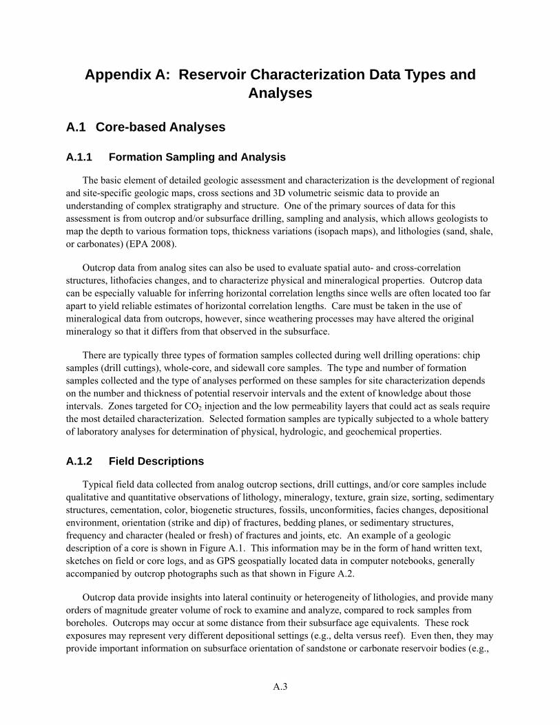
The basic element of detailed geologic assessment and characterization is the development of regional and site-specific geologic maps, cross sections and 3D volumetric seismic data to provide an understanding of complex stratigraphy and structure. One of the primary sources of data for this assessment is from outcrop and/or subsurface drilling, sampling and analysis, which allows geologists to map the depth to various formation tops, thickness variations (isopach maps), and lithologies (sand, shale, or carbonates) (EPA 2008).

Outcrop data from analog sites can also be used to evaluate spatial auto- and cross-correlation structures, lithofacies changes, and to characterize physical and mineralogical properties. Outcrop data can be especially valuable for inferring horizontal correlation lengths since wells are often located too far apart to yield reliable estimates of horizontal correlation lengths. Care must be taken in the use of mineralogical data from outcrops, however, since weathering processes may have altered the original mineralogy so that it differs from that observed in the subsurface.

There are typically three types of formation samples collected during well drilling operations: chip samples (drill cuttings), whole-core, and sidewall core samples. The type and number of formation samples collected and the type of analyses performed on these samples for site characterization depends on the number and thickness of potential reservoir intervals and the extent of knowledge about those intervals. Zones targeted for CO2 injection and the low permeability layers that could act as seals require the most detailed characterization. Selected formation samples are typically subjected to a whole battery of laboratory analyses for determination of physical, hydrologic, and geochemical properties.

A.1.2 Field Descriptions

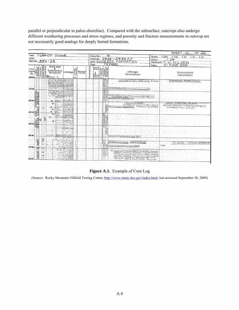
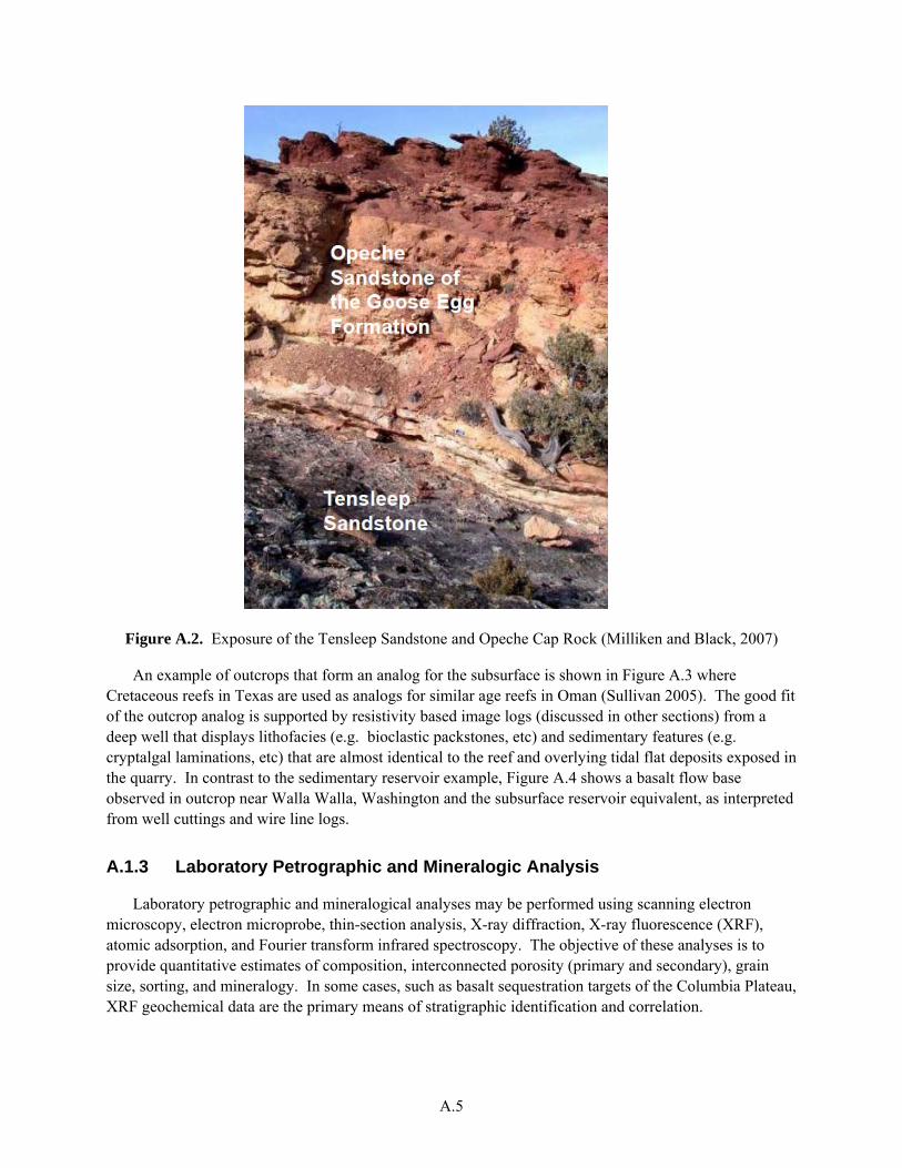
Typical field data collected from analog outcrop sections, drill cuttings, and/or core samples include qualitative and quantitative observations of lithology, mineralogy, texture, grain size, sorting, sedimentary structures, cementation, color, biogenetic structures, fossils, unconformities, facies changes, depositional environment, orientation (strike and dip) of fractures, bedding planes, or sedimentary structures, frequency and character (healed or fresh) of fractures and joints, etc. An example of a geologic description of a core is shown in Figure A.1. This information may be in the form of hand written text, sketches on field or core logs, and as GPS geospatially located data in computer notebooks, generally accompanied by outcrop photographs such as that shown in Figure A.2.

Outcrop data provide insights into lateral continuity or heterogeneity of lithologies, and provide many orders of magnitude greater volume of rock to examine and analyze, compared to rock samples from boreholes. Outcrops may occur at some distance from their subsurface age equivalents. These rock exposures may represent very different depositional settings (e.g., delta versus reef). Even then, they may provide important information on subsurface orientation of sandstone or carbonate reservoir bodies (e.g.,

A.4

parallel or perpendicular to paleo-shoreline). Compared with the subsurface, outcrops also undergo different weathering processes and stress regimes, and porosity and fracture measurements in outcrop are not necessarily good analogs for deeply buried formations.

Figure A.1. Example of Core Log (Source: Rocky Mountain Oilfield Testing Center, http://www.rmotc.doe.gov/index.html, last accessed September 30, 2009)

A.5

Figure A.2. Exposure of the Tensleep Sandstone and Opeche Cap Rock (Milliken and Black, 2007)

An example of outcrops that form an analog for the subsurface is shown in Figure A.3 where Cretaceous reefs in Texas are used as analogs for similar age reefs in Oman (Sullivan 2005). The good fit of the outcrop analog is supported by resistivity based image logs (discussed in other sections) from a deep well that displays lithofacies (e.g. bioclastic packstones, etc) and sedimentary features (e.g. cryptalgal laminations, etc) that are almost identical to the reef and overlying tidal flat deposits exposed in the quarry. In contrast to the sedimentary reservoir example, Figure A.4 shows a basalt flow base observed in outcrop near Walla Walla, Washington and the subsurface reservoir equivalent, as interpreted from well cuttings and wire line logs.

A.1.3 Laboratory Petrographic and Mineralogic Analysis

Laboratory petrographic and mineralogical analyses may be performed using scanning electron microscopy, electron microprobe, thin-section analysis, X-ray diffraction, X-ray fluorescence (XRF), atomic adsorption, and Fourier transform infrared spectroscopy. The objective of these analyses is to provide quantitative estimates of composition, interconnected porosity (primary and secondary), grain size, sorting, and mineralogy. In some cases, such as basalt sequestration targets of the Columbia Plateau, XRF geochemical data are the primary means of stratigraphic identification and correlation.

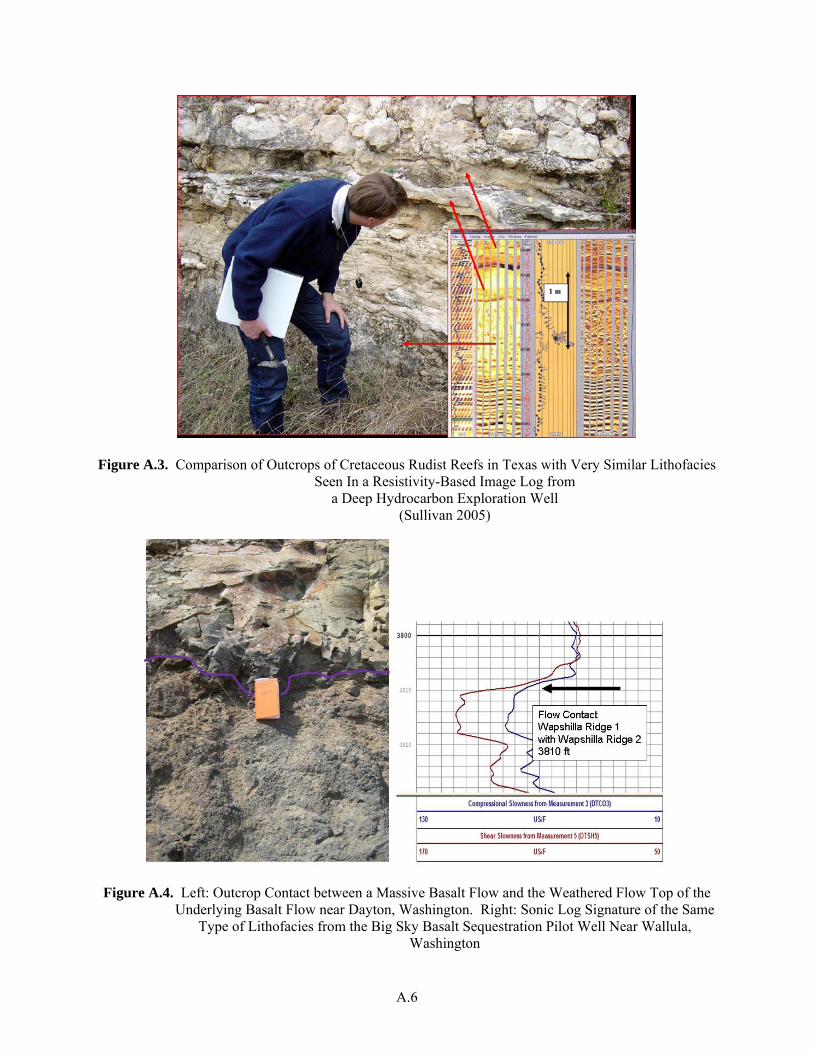
A.6

Figure A.3. Comparison of Outcrops of Cretaceous Rudist Reefs in Texas with Very Similar Lithofacies Seen In a Resistivity-Based Image Log from

a Deep Hydrocarbon Exploration Well (Sullivan 2005)

Figure A.4. Left: Outcrop Contact between a Massive Basalt Flow and the Weathered Flow Top of the Underlying Basalt Flow near Dayton, Washington. Right: Sonic Log Signature of the Same

Type of Lithofacies from the Big Sky Basalt Sequestration Pilot Well Near Wallula, Washington

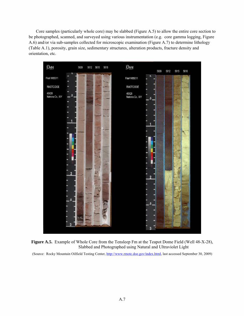
A.7

Core samples (particularly whole core) may be slabbed (Figure A.5) to allow the entire core section to be photographed, scanned, and surveyed using various instrumentation (e.g. core gamma logging, Figure A.6) and/or via sub-samples collected for microscopic examination (Figure A.7) to determine lithology (Table A.1), porosity, grain size, sedimentary structures, alteration products, fracture density and orientation, etc.

Figure A.5. Example of Whole Core from the Tensleep Fm at the Teapot Dome Field (Well 48-X-28), Slabbed and Photographed using Natural and Ultraviolet Light

(Source: Rocky Mountain Oilfield Testing Center, http://www.rmotc.doe.gov/index.html, last accessed September 30, 2009)

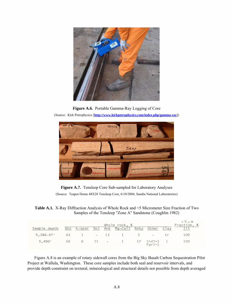
A.8

Figure A.6. Portable Gamma-Ray Logging of Core (Source: Kirk Petrophysics [http://www.kirkpetrophysics.com/index.php/gamma-ray])

Figure A.7. Tensleep Core Sub-sampled for Laboratory Analyses (Source: Teapot Dome 48X28 Tensleep Core, 6/10/2004, Sandia National Laboratories)

Table A.1. X-Ray Diffraction Analysis of Whole Rock and <5 Micrometer Size Fraction of Two Samples of the Tensleep "Zone A" Sandstone (Coughlin 1982)

Figure A.8 is an example of rotary sidewall cores from the Big Sky Basalt Carbon Sequestration Pilot Project at Wallula, Washington. These core samples include both seal and reservoir intervals, and provide depth constraint on textural, mineralogical and structural details not possible from depth averaged

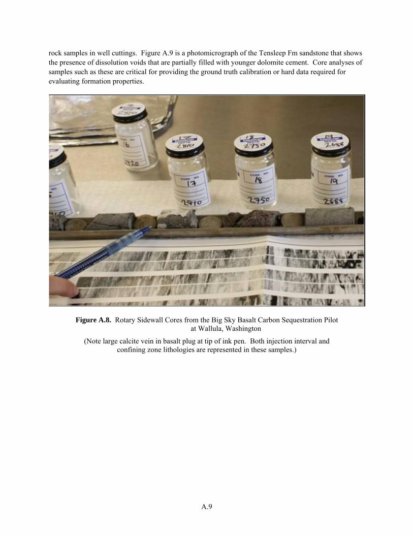
A.9

rock samples in well cuttings. Figure A.9 is a photomicrograph of the Tensleep Fm sandstone that shows the presence of dissolution voids that are partially filled with younger dolomite cement. Core analyses of samples such as these are critical for providing the ground truth calibration or hard data required for evaluating formation properties.

Figure A.8. Rotary Sidewall Cores from the Big Sky Basalt Carbon Sequestration Pilot at Wallula, Washington

(Note large calcite vein in basalt plug at tip of ink pen. Both injection interval and confining zone lithologies are represented in these samples.)

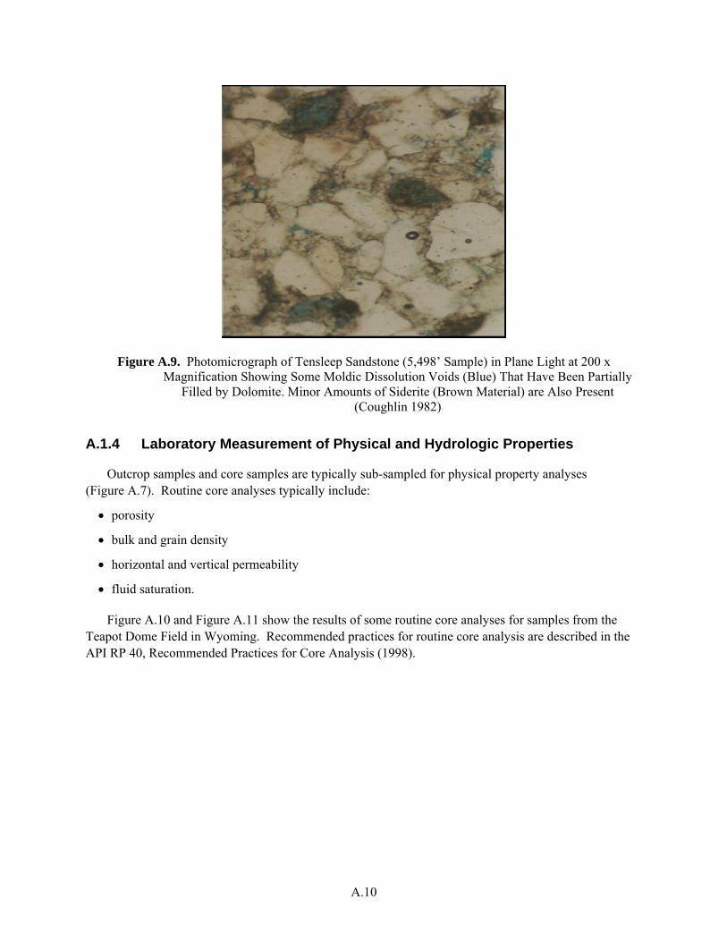
A.10

Figure A.9. Photomicrograph of Tensleep Sandstone (5,498’ Sample) in Plane Light at 200 x Magnification Showing Some Moldic Dissolution Voids (Blue) That Have Been Partially

Filled by Dolomite. Minor Amounts of Siderite (Brown Material) are Also Present (Coughlin 1982)

A.1.4 Laboratory Measurement of Physical and Hydrologic Properties

Outcrop samples and core samples are typically sub-sampled for physical property analyses (Figure A.7). Routine core analyses typically include:

• porosity

• bulk and grain density

• horizontal and vertical permeability

• fluid saturation.

Figure A.10 and Figure A.11 show the results of some routine core analyses for samples from the Teapot Dome Field in Wyoming. Recommended practices for routine core analysis are described in the API RP 40, Recommended Practices for Core Analysis (1998).

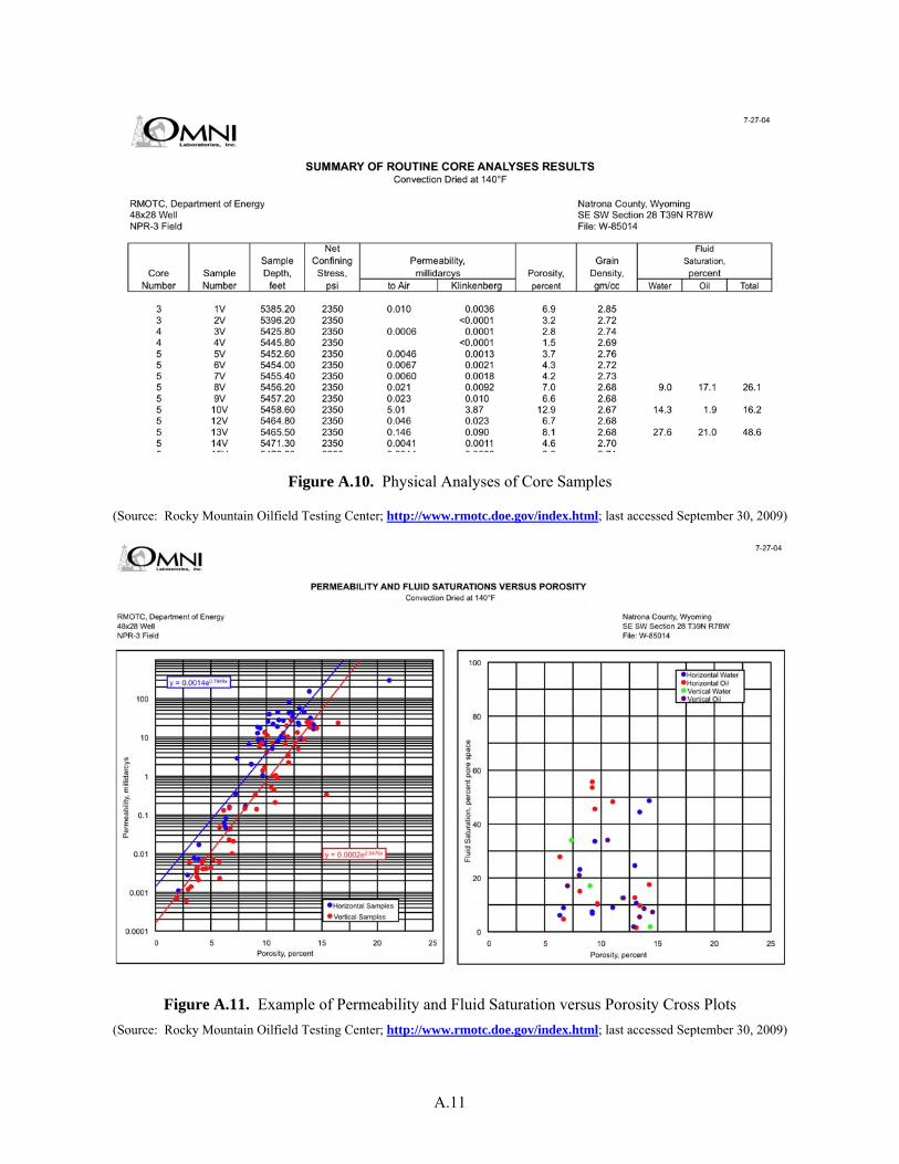
A.11

Figure A.10. Physical Analyses of Core Samples

(Source: Rocky Mountain Oilfield Testing Center; http://www.rmotc.doe.gov/index.html; last accessed September 30, 2009)

Figure A.11. Example of Permeability and Fluid Saturation versus Porosity Cross Plots (Source: Rocky Mountain Oilfield Testing Center; http://www.rmotc.doe.gov/index.html; last accessed September 30, 2009)

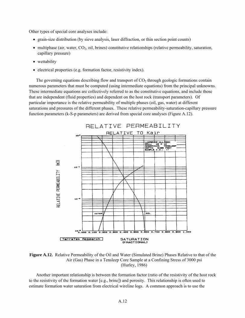
A.12

Other types of special core analyses include:

• grain-size distribution (by sieve analysis, laser diffraction, or thin section point counts)

• multiphase (air, water, CO2, oil, brines) constitutive relationships (relative permeability, saturation, capillary pressure)

• wettability

• electrical properties (e.g. formation factor, resistivity index).

The governing equations describing flow and transport of CO2 through geologic formations contain numerous parameters that must be computed (using intermediate equations) from the principal unknowns. These intermediate equations are collectively referred to as the constitutive equations, and include those that are independent (fluid properties) and dependent on the host rock (transport parameters). Of particular importance is the relative permeability of multiple phases (oil, gas, water) at different saturations and pressures of the different phases. These relative permeability-saturation-capillary pressure function parameters (k-S-p parameters) are derived from special core analyses (Figure A.12).

Figure A.12. Relative Permeability of the Oil and Water (Simulated Brine) Phases Relative to that of the Air (Gas) Phase in a Tensleep Core Sample at a Confining Stress of 3000 psi

(Hurley, 1986)

Another important relationship is between the formation factor (ratio of the resistivity of the host rock to the resistivity of the formation water [e.g., brine]) and porosity. This relationship is often used to estimate formation water saturation from electrical wireline logs. A common approach is to use the

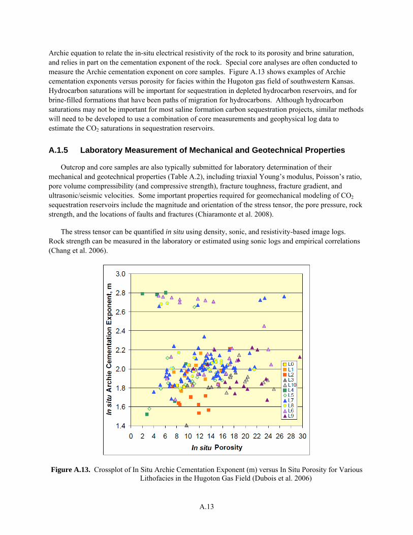
A.13

Archie equation to relate the in-situ electrical resistivity of the rock to its porosity and brine saturation, and relies in part on the cementation exponent of the rock. Special core analyses are often conducted to measure the Archie cementation exponent on core samples. Figure A.13 shows examples of Archie cementation exponents versus porosity for facies within the Hugoton gas field of southwestern Kansas. Hydrocarbon saturations will be important for sequestration in depleted hydrocarbon reservoirs, and for brine-filled formations that have been paths of migration for hydrocarbons. Although hydrocarbon saturations may not be important for most saline formation carbon sequestration projects, similar methods will need to be developed to use a combination of core measurements and geophysical log data to estimate the CO2 saturations in sequestration reservoirs.

A.1.5 Laboratory Measurement of Mechanical and Geotechnical Properties

Outcrop and core samples are also typically submitted for laboratory determination of their mechanical and geotechnical properties (Table A.2), including triaxial Young’s modulus, Poisson’s ratio, pore volume compressibility (and compressive strength), fracture toughness, fracture gradient, and ultrasonic/seismic velocities. Some important properties required for geomechanical modeling of CO2 sequestration reservoirs include the magnitude and orientation of the stress tensor, the pore pressure, rock strength, and the locations of faults and fractures (Chiaramonte et al. 2008).

The stress tensor can be quantified in situ using density, sonic, and resistivity-based image logs. Rock strength can be measured in the laboratory or estimated using sonic logs and empirical correlations (Chang et al. 2006).

Figure A.13. Crossplot of In Situ Archie Cementation Exponent (m) versus In Situ Porosity for Various Lithofacies in the Hugoton Gas Field (Dubois et al. 2006)

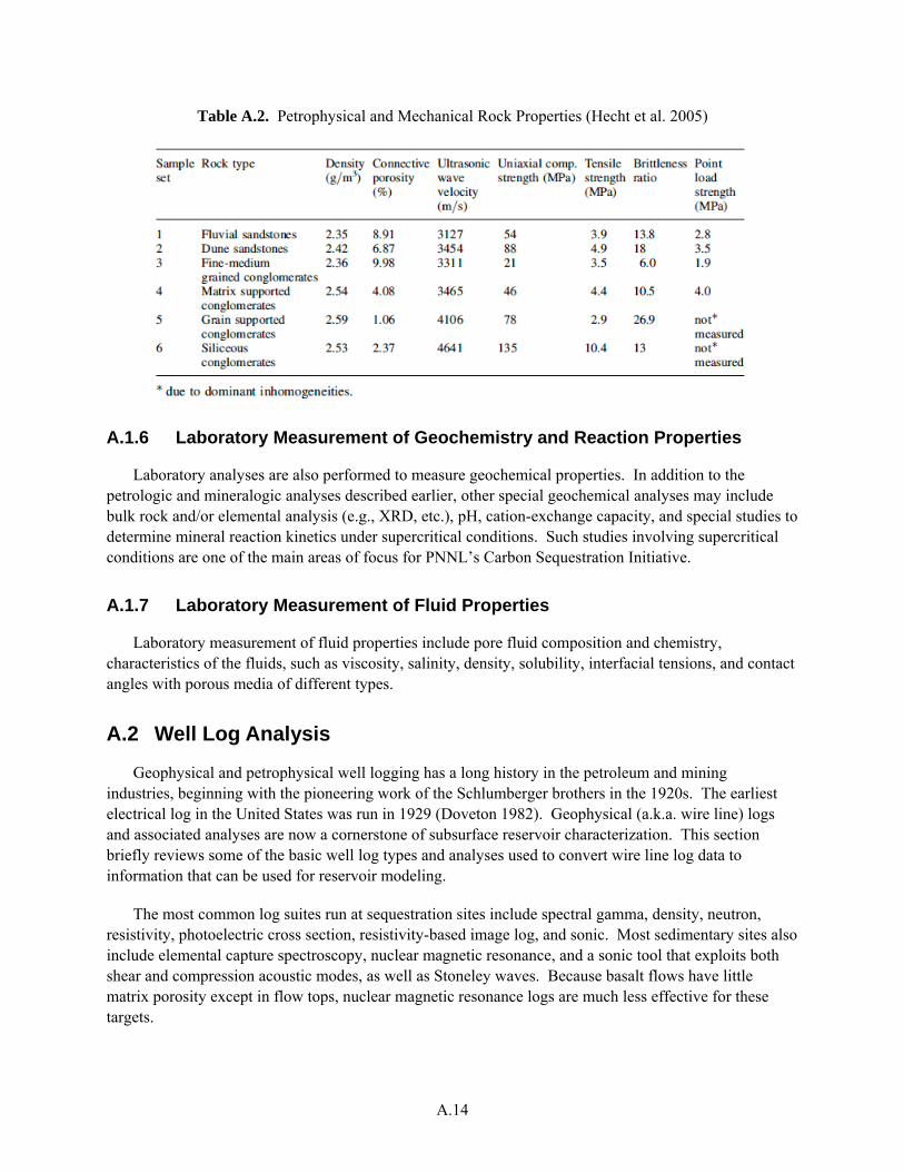
A.14

Table A.2. Petrophysical and Mechanical Rock Properties (Hecht et al. 2005)

A.1.6 Laboratory Measurement of Geochemistry and Reaction Properties

Laboratory analyses are also performed to measure geochemical properties. In addition to the petrologic and mineralogic analyses described earlier, other special geochemical analyses may include bulk rock and/or elemental analysis (e.g., XRD, etc.), pH, cation-exchange capacity, and special studies to determine mineral reaction kinetics under supercritical conditions. Such studies involving supercritical conditions are one of the main areas of focus for PNNL’s Carbon Sequestration Initiative.

A.1.7 Laboratory Measurement of Fluid Properties

Laboratory measurement of fluid properties include pore fluid composition and chemistry, characteristics of the fluids, such as viscosity, salinity, density, solubility, interfacial tensions, and contact angles with porous media of different types.

A.2 Well Log Analysis

Geophysical and petrophysical well logging has a long history in the petroleum and mining industries, beginning with the pioneering work of the Schlumberger brothers in the 1920s. The earliest electrical log in the United States was run in 1929 (Doveton 1982). Geophysical (a.k.a. wire line) logs and associated analyses are now a cornerstone of subsurface reservoir characterization. This section briefly reviews some of the basic well log types and analyses used to convert wire line log data to information that can be used for reservoir modeling.

The most common log suites run at sequestration sites include spectral gamma, density, neutron, resistivity, photoelectric cross section, resistivity-based image log, and sonic. Most sedimentary sites also include elemental capture spectroscopy, nuclear magnetic resonance, and a sonic tool that exploits both shear and compression acoustic modes, as well as Stoneley waves. Because basalt flows have little matrix porosity except in flow tops, nuclear magnetic resonance logs are much less effective for these targets.

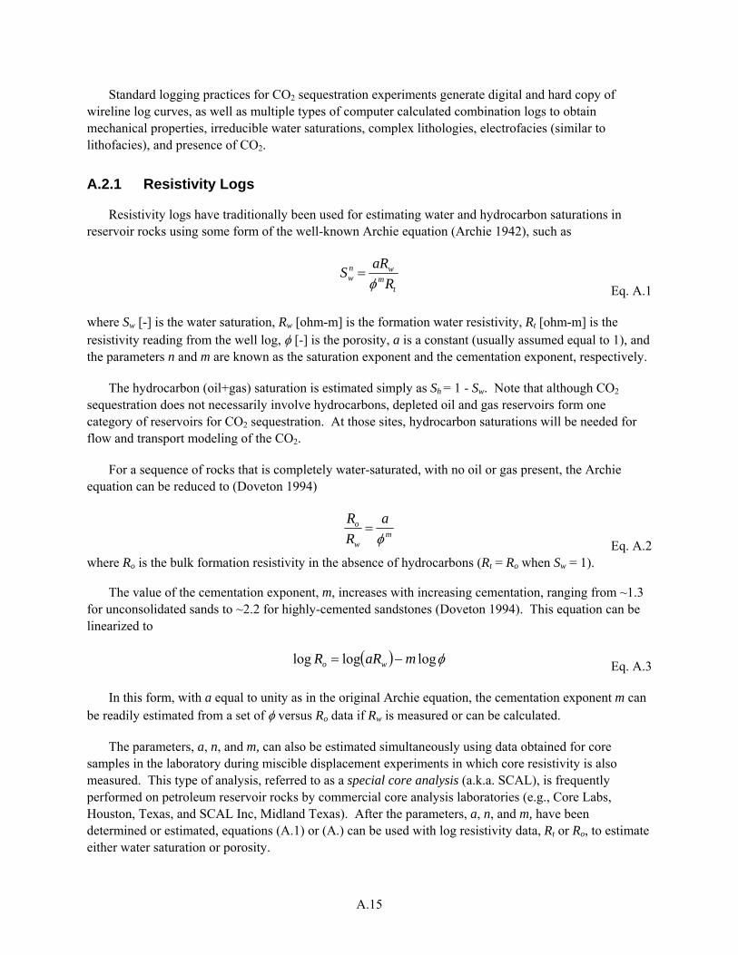
A.15

Standard logging practices for CO2 sequestration experiments generate digital and hard copy of wireline log curves, as well as multiple types of computer calculated combination logs to obtain mechanical properties, irreducible water saturations, complex lithologies, electrofacies (similar to lithofacies), and presence of CO2.

A.2.1 Resistivity Logs

Resistivity logs have traditionally been used for estimating water and hydrocarbon saturations in reservoir rocks using some form of the well-known Archie equation (Archie 1942), such as

tm

wnw R

aRSφ

= Eq. A.1

where Sw [-] is the water saturation, Rw [ohm-m] is the formation water resistivity, Rt [ohm-m] is the resistivity reading from the well log, φ [-] is the porosity, a is a constant (usually assumed equal to 1), and the parameters n and m are known as the saturation exponent and the cementation exponent, respectively.

The hydrocarbon (oil+gas) saturation is estimated simply as Sh = 1 - Sw. Note that although CO2 sequestration does not necessarily involve hydrocarbons, depleted oil and gas reservoirs form one category of reservoirs for CO2 sequestration. At those sites, hydrocarbon saturations will be needed for flow and transport modeling of the CO2.

For a sequence of rocks that is completely water-saturated, with no oil or gas present, the Archie equation can be reduced to (Doveton 1994)

m

w

o aRR

φ=

Eq. A.2 where Ro is the bulk formation resistivity in the absence of hydrocarbons (Rt = Ro when Sw = 1).

The value of the cementation exponent, m, increases with increasing cementation, ranging from ~1.3 for unconsolidated sands to ~2.2 for highly-cemented sandstones (Doveton 1994). This equation can be linearized to

( ) φlogloglog maRR wo −= Eq. A.3

In this form, with a equal to unity as in the original Archie equation, the cementation exponent m can be readily estimated from a set of φ versus Ro data if Rw is measured or can be calculated.

The parameters, a, n, and m, can also be estimated simultaneously using data obtained for core samples in the laboratory during miscible displacement experiments in which core resistivity is also measured. This type of analysis, referred to as a special core analysis (a.k.a. SCAL), is frequently performed on petroleum reservoir rocks by commercial core analysis laboratories (e.g., Core Labs, Houston, Texas, and SCAL Inc, Midland Texas). After the parameters, a, n, and m, have been determined or estimated, equations (A.1) or (A.) can be used with log resistivity data, Rt or Ro, to estimate either water saturation or porosity.

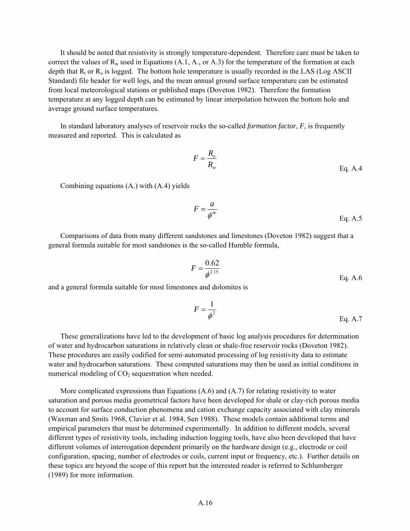
A.16

It should be noted that resistivity is strongly temperature-dependent. Therefore care must be taken to correct the values of Rw used in Equations (A.1, A., or A.3) for the temperature of the formation at each depth that Rt or Ro is logged. The bottom hole temperature is usually recorded in the LAS (Log ASCII Standard) file header for well logs, and the mean annual ground surface temperature can be estimated from local meteorological stations or published maps (Doveton 1982). Therefore the formation temperature at any logged depth can be estimated by linear interpolation between the bottom hole and average ground surface temperatures.

In standard laboratory analyses of reservoir rocks the so-called formation factor, F, is frequently measured and reported. This is calculated as

w

o

RRF =

Eq. A.4

Combining equations (A.) with (A.4) yields

m

aFφ

= Eq. A.5

Comparisons of data from many different sandstones and limestones (Doveton 1982) suggest that a general formula suitable for most sandstones is the so-called Humble formula,

15.2

62.0φ

=F Eq. A.6

and a general formula suitable for most limestones and dolomites is

2

1φ

=F Eq. A.7

These generalizations have led to the development of basic log analysis procedures for determination of water and hydrocarbon saturations in relatively clean or shale-free reservoir rocks (Doveton 1982). These procedures are easily codified for semi-automated processing of log resistivity data to estimate water and hydrocarbon saturations. These computed saturations may then be used as initial conditions in numerical modeling of CO2 sequestration when needed.

More complicated expressions than Equations (A.6) and (A.7) for relating resistivity to water saturation and porous media geometrical factors have been developed for shale or clay-rich porous media to account for surface conduction phenomena and cation exchange capacity associated with clay minerals (Waxman and Smits 1968, Clavier et al. 1984, Sen 1988). These models contain additional terms and empirical parameters that must be determined experimentally. In addition to different models, several different types of resistivity tools, including induction logging tools, have also been developed that have different volumes of interrogation dependent primarily on the hardware design (e.g., electrode or coil configuration, spacing, number of electrodes or coils, current input or frequency, etc.). Further details on these topics are beyond the scope of this report but the interested reader is referred to Schlumberger (1989) for more information.

A.17

A.2.1.1 Resistivity-Based Image Logs

The resistivity-based image logging tool has six arms that press resistivity-measuring sensors against the rock wall of the borehole. This tool provides up to 80% coverage of the borehole (for an 8" diameter hole). More resistive areas corresponding to low porosity are conventionally assigned a light yellow color. Darker brown areas are less resistive and indicate clays or microporosity with bound water, or open porosity filled with water. The data provide texture and azimuthal oriented fracture and stratigraphic dip data with a 1/8 inch resolution. These data are extremely powerful in determining maximum and minimum horizontal stress tensors, dip and strike orientation of bedforms and structure, such as ripples, faults, bedding planes, natural and healed fractures, as well as textures that help identify a multitude of lithofacies and porosity types. Image log data are important for building reservoir models for both basalt and sedimentary sequestration projects.

Image logs are one of the most important tools in log-based, stratigraphic analysis of internal reservoir architecture. Figure A.14 is an image log segment that shows a series of thin sedimentary carbonate layers that formed in a shallow water, reefal environment. The column on left shows the entire logged interval with the gamma log curve superimposed on the image log. The second and fourth tracks show enlargements of the static and enhanced images of the narrow green segment of the logged interval shown in the left track. Note the scale of one meter between depth marks on the enlarged section. The "tadpoles" in the third track show stratigraphic dip by the head of the tadpole, and dip azimuth with the tadpole tale. Zero dip (horizontal) is to the left of the track, 90 degrees (vertical) dip is to the right. No structural fractures are present in this log segment. This image shows very thin, low dip (almost horizontal) carbonate beds overlain by fossiliferous carbonates that have vuggy porosity due to dissolution of fossils. The upper portion of the image is interpreted as tidal flat microbial mat deposits. The lithologies have been verified from rock cuttings and signatures on computed log suites.

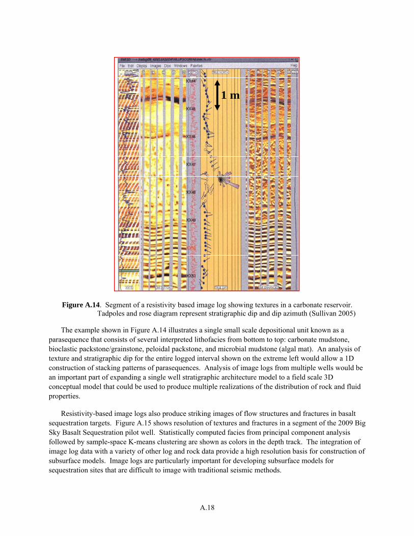
A.18

1 m1 m

Figure A.14. Segment of a resistivity based image log showing textures in a carbonate reservoir. Tadpoles and rose diagram represent stratigraphic dip and dip azimuth (Sullivan 2005)

The example shown in Figure A.14 illustrates a single small scale depositional unit known as a parasequence that consists of several interpreted lithofacies from bottom to top: carbonate mudstone, bioclastic packstone/grainstone, peloidal packstone, and microbial mudstone (algal mat). An analysis of texture and stratigraphic dip for the entire logged interval shown on the extreme left would allow a 1D construction of stacking patterns of parasequences. Analysis of image logs from multiple wells would be an important part of expanding a single well stratigraphic architecture model to a field scale 3D conceptual model that could be used to produce multiple realizations of the distribution of rock and fluid properties.

Resistivity-based image logs also produce striking images of flow structures and fractures in basalt sequestration targets. Figure A.15 shows resolution of textures and fractures in a segment of the 2009 Big Sky Basalt Sequestration pilot well. Statistically computed facies from principal component analysis followed by sample-space K-means clustering are shown as colors in the depth track. The integration of image log data with a variety of other log and rock data provide a high resolution basis for construction of subsurface models. Image logs are particularly important for developing subsurface models for sequestration sites that are difficult to image with traditional seismic methods.

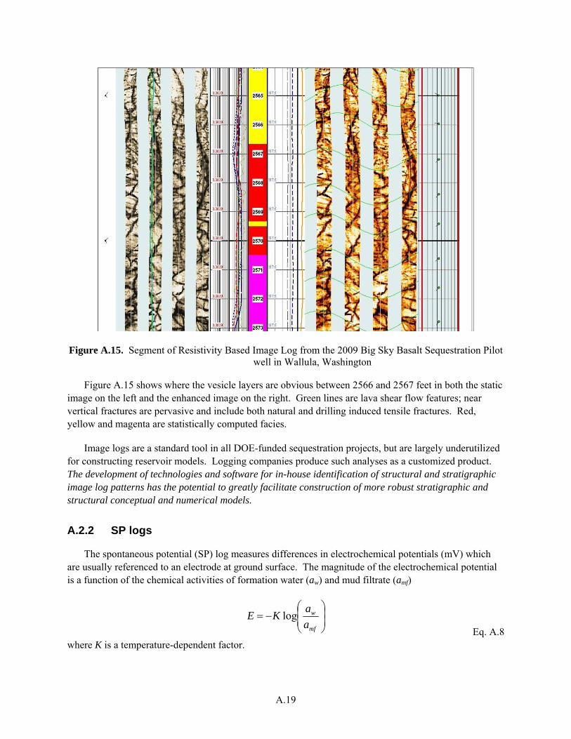
A.19

Figure A.15. Segment of Resistivity Based Image Log from the 2009 Big Sky Basalt Sequestration Pilot well in Wallula, Washington

Figure A.15 shows where the vesicle layers are obvious between 2566 and 2567 feet in both the static image on the left and the enhanced image on the right. Green lines are lava shear flow features; near vertical fractures are pervasive and include both natural and drilling induced tensile fractures. Red, yellow and magenta are statistically computed facies.

Image logs are a standard tool in all DOE-funded sequestration projects, but are largely underutilized for constructing reservoir models. Logging companies produce such analyses as a customized product. The development of technologies and software for in-house identification of structural and stratigraphic image log patterns has the potential to greatly facilitate construction of more robust stratigraphic and structural conceptual and numerical models.

A.2.2 SP logs

The spontaneous potential (SP) log measures differences in electrochemical potentials (mV) which are usually referenced to an electrode at ground surface. The magnitude of the electrochemical potential is a function of the chemical activities of formation water (aw) and mud filtrate (amf)

⎟⎟⎠

⎞⎜⎜⎝

⎛−=

mf

w

aaKE log

Eq. A.8 where K is a temperature-dependent factor.

A.20

The chemical activity of a single-salt solution is proportional to the salt concentration, which is inversely related to the solution resistivity. If the drilling fluid (a.k.a. mud) filtrate and formation waters are approximated by pure sodium chloride solutions, the equation becomes (Doveton 1982)

⎟⎟⎠

⎞⎜⎜⎝

⎛−=

w

mf

RR

KE log Eq. A.9

The general features of the SP log are as follows (Doveton 1982):

1. When the drilling mud is fresh water (i.e., Rmf > Rw), then the SP log shows a shift to the negative when moving from a shale to a permeable formation;

2. When the drilling fluid is a salt mud (i.e., Rmf < Rw) the SP log is displaced in a positive direction when moving from a shale to a permeable formation;

3. The magnitude of the shift is a function of the resistivity contrast between the mud filtrate and the formation water;

4. The SP log can be used to estimate formation water resistivity (via Eq. A.9) since the formation temperature can be estimated, giving a value for K, and the mud filtrate resistivity is typically measured at the well site.

For boreholes with fresh mud, shales and permeable formations read as relatively positive and negative SP values, respectively.

One SP-related calculation of interest is the difference between the potentials of the shale and the clean (shale-free) permeable formation. This quantity is known as the static self-potential, or SSP. In shaley, permeable formations the displacement of the SP log from the shale reading is also of interest and is referred to as a pseudo-static potential, or PSP. The relationship between PSP and SSP is a function of shale content and is expressed as

SSPPSP /=α Eq. A.10

The SP log, scaled in terms of α, is often used as one of several shale indicators, where (1 - α) is an estimate of the fractional shale content (Doveton 1982).

A.2.3 Neutron Log

Neutron logging tools generate high-energy neutrons, typically from an americium-beryllium source, that radiate into a formation and collide with the nuclei of atoms that they encounter. These collisions result in a reduction in energy that is measured by one or several detectors on the neutron logging tool. The greatest energy loss is caused by collisions with nuclei of like mass within the formation—principally hydrogen atoms—such that the neutron log effectively measures hydrogen contained in both the pore fluids and in chemically bound water. In clean liquid-filled formations, neutron log measurements primarily reflect the amount of liquid-filled porosity. Gypsiferous rocks (e.g., CaSO4⋅nH2O) can produce neutron porosity values that are higher than the actual porosity that is present due to the presence of bound water. Hence, whenever significant quantities of gypsum are expected to be present, as in the case of the shallow geology of the 2006 proposed west Texas FutureGen site (McGrail et al. 2006d) or the

A.21

Permian Tensleep sandstones of Wyoming the use of multiple porosity logs is recommended (Savre 1963).

The Schlumberger compensated neutron log (CNL) is a dual-spacing, thermal neutron-detection instrument that is sensitive to shale because shales usually contain small amounts of boron and other rare earth elements that have very high thermal neutron capture cross sections (Schlumberger 1989). In addition to thermal neutron detectors, the dual-energy neutron log (DNL) also incorporates two epithermal neutron detectors that allow for two different porosity measurements to be obtained. In clean formations these two measurements generally agree, while in shaley formations the porosity measured by the epithermal detectors is generally lower and agrees more closely with density-derived porosity (Schlumberger 1989). Differences in the two porosity measurements can be used as a measure of shale or clay content, or of formation fluid salinity. The DNL tool also yields improved gas detection in shaley reservoirs.

Neutron-porosity values estimated from neutron logs, as well as some other types of logs such as the gamma ray log, are typically reported in American Petroleum Institute (API) units based on calibration standards for limestone or sandstone from a test facility in Houston, Texas.

A.2.3.1 Pulsed Neutron Sigma Logs

Pulsed neutron logs, such as the Schlumberger RST (reservoir saturation) tool, provide measurements of formation capture cross-section porosity and carbon/oxygen spectroscopy. The tool records thermal decay time and has been adapted from oilfield use to the detection and quantification of reservoir saturations of injected CO2. The Sigma log, which uses time-lapse RST logs, is one of the few tools able to quantify residual saturations of CO2. The residual saturation trapping mechanism has important implications for sequestration: if CO2 is injected near the base of a thick (100s of feet) porous reservoir, much of the CO2 might become stranded or permanently sequestered after moving upward through a distance equivalent to about 10 or 20 pore volumes.

The application of the time lapse RST tool was pioneered at the Frio sequestration test site (Hovorka et al. 2005), where time lapse Sigma logs (Figure A.16) first indicated a residual saturation of 20% of CO2 in the poorly consolidated Frio sandstones after CO2 had passed through the reservoir. Although other analyses have indicated that the residual (immovable) saturation might be closer to 10%, the sigma log measurements represent one of the most promising areas of research in data assimilation for quantifying saturations and calibrating vertical seismic profile (VSP), cross well and surface based seismic signatures.

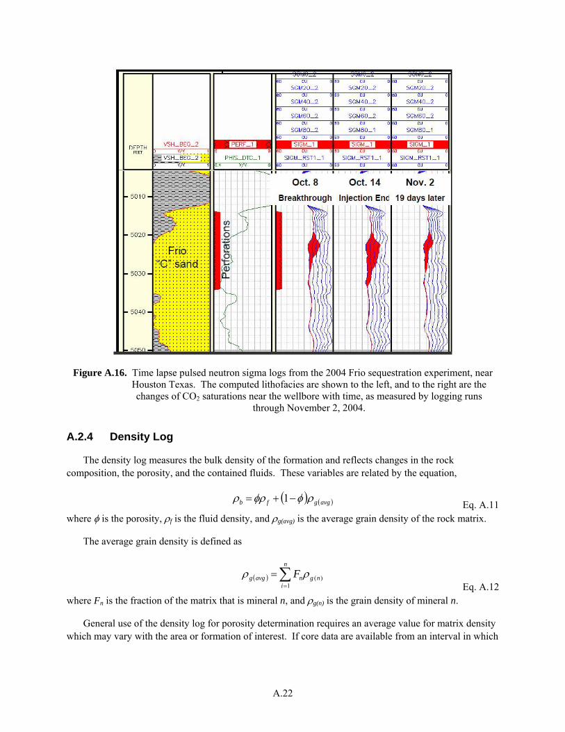
A.22

Figure A.16. Time lapse pulsed neutron sigma logs from the 2004 Frio sequestration experiment, near Houston Texas. The computed lithofacies are shown to the left, and to the right are the changes of CO2 saturations near the wellbore with time, as measured by logging runs

through November 2, 2004.

A.2.4 Density Log

The density log measures the bulk density of the formation and reflects changes in the rock composition, the porosity, and the contained fluids. These variables are related by the equation,

( ) ( )avggfb ρφφρρ −+= 1 Eq. A.11 where φ is the porosity, ρf is the fluid density, and ρg(avg) is the average grain density of the rock matrix.

The average grain density is defined as

( ) ∑

=

=n

ingnavgg F

1)(ρρ Eq. A.12

where Fn is the fraction of the matrix that is mineral n, and ρg(n) is the grain density of mineral n.

General use of the density log for porosity determination requires an average value for matrix density which may vary with the area or formation of interest. If core data are available from an interval in which

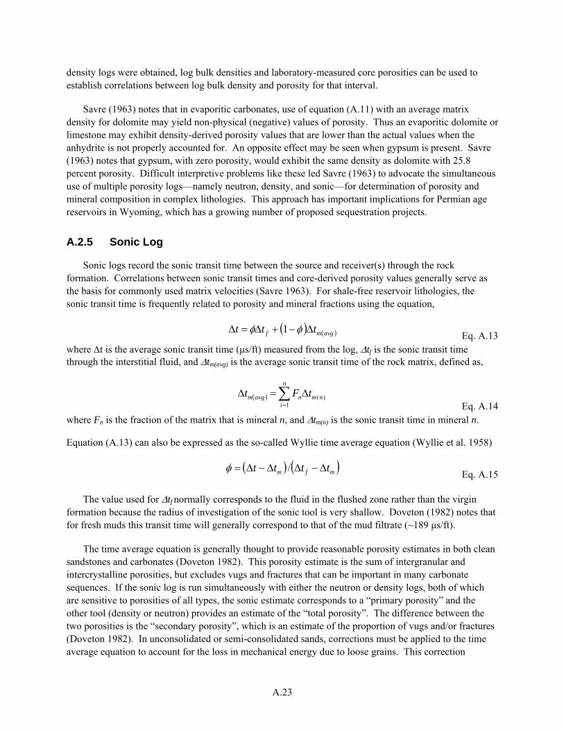
A.23

density logs were obtained, log bulk densities and laboratory-measured core porosities can be used to establish correlations between log bulk density and porosity for that interval.

Savre (1963) notes that in evaporitic carbonates, use of equation (A.11) with an average matrix density for dolomite may yield non-physical (negative) values of porosity. Thus an evaporitic dolomite or limestone may exhibit density-derived porosity values that are lower than the actual values when the anhydrite is not properly accounted for. An opposite effect may be seen when gypsum is present. Savre (1963) notes that gypsum, with zero porosity, would exhibit the same density as dolomite with 25.8 percent porosity. Difficult interpretive problems like these led Savre (1963) to advocate the simultaneous use of multiple porosity logs—namely neutron, density, and sonic—for determination of porosity and mineral composition in complex lithologies. This approach has important implications for Permian age reservoirs in Wyoming, which has a growing number of proposed sequestration projects.

A.2.5 Sonic Log

Sonic logs record the sonic transit time between the source and receiver(s) through the rock formation. Correlations between sonic transit times and core-derived porosity values generally serve as the basis for commonly used matrix velocities (Savre 1963). For shale-free reservoir lithologies, the sonic transit time is frequently related to porosity and mineral fractions using the equation,

( ) ( )avgmf ttt Δ−+Δ=Δ φφ 1 Eq. A.13 where Δt is the average sonic transit time (μs/ft) measured from the log, Δtf is the sonic transit time through the interstitial fluid, and Δtm(avg) is the average sonic transit time of the rock matrix, defined as,

( ) ∑

=

Δ=Δn

inmnavgm tFt

1)(

Eq. A.14 where Fn is the fraction of the matrix that is mineral n, and Δtm(n) is the sonic transit time in mineral n.

Equation (A.13) can also be expressed as the so-called Wyllie time average equation (Wyllie et al. 1958)

( ) ( )mfm tttt Δ−ΔΔ−Δ= /φ Eq. A.15

The value used for Δtf normally corresponds to the fluid in the flushed zone rather than the virgin formation because the radius of investigation of the sonic tool is very shallow. Doveton (1982) notes that for fresh muds this transit time will generally correspond to that of the mud filtrate (~189 μs/ft).

The time average equation is generally thought to provide reasonable porosity estimates in both clean sandstones and carbonates (Doveton 1982). This porosity estimate is the sum of intergranular and intercrystalline porosities, but excludes vugs and fractures that can be important in many carbonate sequences. If the sonic log is run simultaneously with either the neutron or density logs, both of which are sensitive to porosities of all types, the sonic estimate corresponds to a “primary porosity” and the other tool (density or neutron) provides an estimate of the “total porosity”. The difference between the two porosities is the “secondary porosity”, which is an estimate of the proportion of vugs and/or fractures (Doveton 1982). In unconsolidated or semi-consolidated sands, corrections must be applied to the time average equation to account for the loss in mechanical energy due to loose grains. This correction

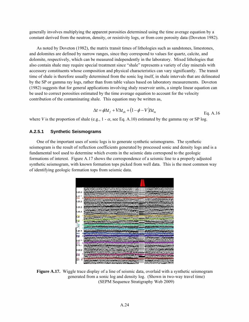
A.24

generally involves multiplying the apparent porosities determined using the time average equation by a constant derived from the neutron, density, or resistivity logs, or from core porosity data (Doveton 1982).

As noted by Doveton (1982), the matrix transit times of lithologies such as sandstones, limestones, and dolomites are defined by narrow ranges, since they correspond to values for quartz, calcite, and dolomite, respectively, which can be measured independently in the laboratory. Mixed lithologies that also contain shale may require special treatment since “shale” represents a variety of clay minerals with accessory constituents whose composition and physical characteristics can vary significantly. The transit time of shale is therefore usually determined from the sonic log itself, in shale intervals that are delineated by the SP or gamma ray logs, rather than from table values based on laboratory measurements. Doveton (1982) suggests that for general applications involving shaly reservoir units, a simple linear equation can be used to correct porosities estimated by the time average equation to account for the velocity contribution of the contaminating shale. This equation may be written as,

( ) mshf tVtVtt Δ−−+Δ+Δ=Δ φφ 1 Eq. A.16 where V is the proportion of shale (e.g., 1 - α, see Eq. A.10) estimated by the gamma ray or SP log.

A.2.5.1 Synthetic Seismograms

One of the important uses of sonic logs is to generate synthetic seismograms. The synthetic seismogram is the result of reflection coefficients generated by processed sonic and density logs and is a fundamental tool used to determine which events in the seismic data correspond to the geologic formations of interest. Figure A.17 shows the correspondence of a seismic line to a properly adjusted synthetic seismogram, with known formation tops picked from well data. This is the most common way of identifying geologic formation tops from seismic data.

Figure A.17. Wiggle trace display of a line of seismic data, overlaid with a synthetic seismogram generated from a sonic log and density log. (Shown in two-way travel time)

(SEPM Sequence Stratigraphy Web 2009)

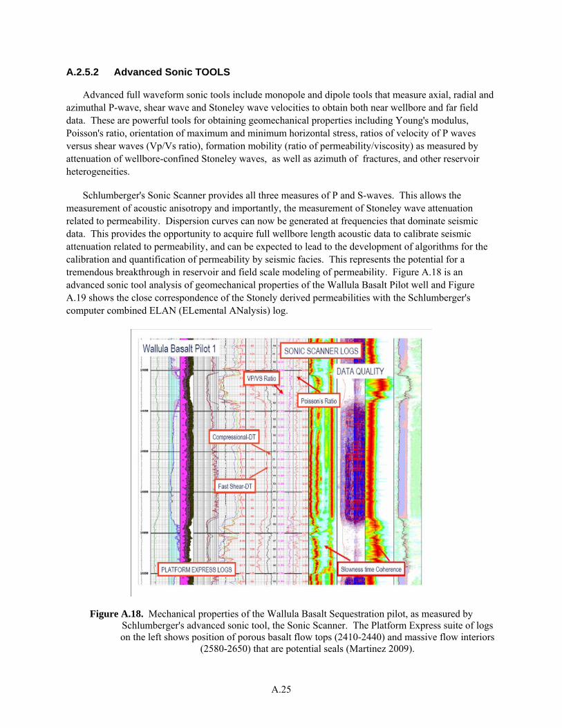
A.25

A.2.5.2 Advanced Sonic TOOLS

Advanced full waveform sonic tools include monopole and dipole tools that measure axial, radial and azimuthal P-wave, shear wave and Stoneley wave velocities to obtain both near wellbore and far field data. These are powerful tools for obtaining geomechanical properties including Young's modulus, Poisson's ratio, orientation of maximum and minimum horizontal stress, ratios of velocity of P waves versus shear waves (Vp/Vs ratio), formation mobility (ratio of permeability/viscosity) as measured by attenuation of wellbore-confined Stoneley waves, as well as azimuth of fractures, and other reservoir heterogeneities.

Schlumberger's Sonic Scanner provides all three measures of P and S-waves. This allows the measurement of acoustic anisotropy and importantly, the measurement of Stoneley wave attenuation related to permeability. Dispersion curves can now be generated at frequencies that dominate seismic data. This provides the opportunity to acquire full wellbore length acoustic data to calibrate seismic attenuation related to permeability, and can be expected to lead to the development of algorithms for the calibration and quantification of permeability by seismic facies. This represents the potential for a tremendous breakthrough in reservoir and field scale modeling of permeability. Figure A.18 is an advanced sonic tool analysis of geomechanical properties of the Wallula Basalt Pilot well and Figure A.19 shows the close correspondence of the Stonely derived permeabilities with the Schlumberger's computer combined ELAN (ELemental ANalysis) log.

Figure A.18. Mechanical properties of the Wallula Basalt Sequestration pilot, as measured by Schlumberger's advanced sonic tool, the Sonic Scanner. The Platform Express suite of logs on the left shows position of porous basalt flow tops (2410-2440) and massive flow interiors

(2580-2650) that are potential seals (Martinez 2009).

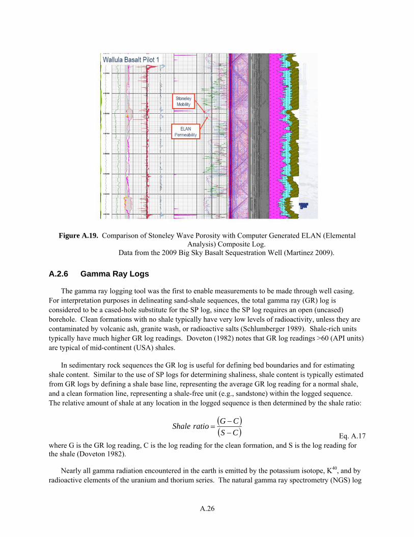
A.26

Figure A.19. Comparison of Stoneley Wave Porosity with Computer Generated ELAN (Elemental Analysis) Composite Log.

Data from the 2009 Big Sky Basalt Sequestration Well (Martinez 2009).

A.2.6 Gamma Ray Logs

The gamma ray logging tool was the first to enable measurements to be made through well casing. For interpretation purposes in delineating sand-shale sequences, the total gamma ray (GR) log is considered to be a cased-hole substitute for the SP log, since the SP log requires an open (uncased) borehole. Clean formations with no shale typically have very low levels of radioactivity, unless they are contaminated by volcanic ash, granite wash, or radioactive salts (Schlumberger 1989). Shale-rich units typically have much higher GR log readings. Doveton (1982) notes that GR log readings >60 (API units) are typical of mid-continent (USA) shales.

In sedimentary rock sequences the GR log is useful for defining bed boundaries and for estimating shale content. Similar to the use of SP logs for determining shaliness, shale content is typically estimated from GR logs by defining a shale base line, representing the average GR log reading for a normal shale, and a clean formation line, representing a shale-free unit (e.g., sandstone) within the logged sequence. The relative amount of shale at any location in the logged sequence is then determined by the shale ratio:

( )( )CS

CGratioShale−−

= Eq. A.17

where G is the GR log reading, C is the log reading for the clean formation, and S is the log reading for the shale (Doveton 1982).

Nearly all gamma radiation encountered in the earth is emitted by the potassium isotope, K40, and by radioactive elements of the uranium and thorium series. The natural gamma ray spectrometry (NGS) log

A.27

measures the concentrations of radioactive potassium, thorium, and uranium. Sedimentary thorium is almost exclusively associated with aluminosilicates and thus the thorium log curve is a good indicator of the volume of clay minerals (Hassan et al. 1976). The thorium/potassium ratio (Th/K) has been used as an indicator of relative potassium richness to distinguish between low-ratio (high-potassium) feldspars and micas and higher ratio illite, smectite, kaolinite, and chlorite (Doveton 1982). The thorium/uranium (Th/U) ratio has been used as an indicator of geochemical facies, with Th/U ratios less than 2 being indicative of reducing conditions and ratios greater than 7 being associated with oxidation (Adams and Weaver 1958, Doveton 1982). Thorium and uranium concentrations are typically reported in units of parts per million (ppm) while K40 concentrations are reported in percent (%). The combination of the NGS log with other lithology-sensitive logs such as the density, neutron, sonic, and photoelectric adsorption logs permit volumetric mineral analysis for very complex lithological mixtures.

A.2.7 Photoelectric Log

The photoelectric (a.k.a. PE or PEF) log is typically recorded as part of the density log measurement. The photoelectric cross-section is a measure of the adsorption of low-energy gamma rays by the formation. According to the Schlumberger Oilfield Glossary (2009), the photoelectric log measures the photoelectric adsorption factor, Pe, of the formation which is defined as (Z/10)3.6, where Z is the average atomic number of the formation. Fluids have very low atomic numbers so Pe is primarily a measure of rock matrix properties. Sandstones typically have relatively low Pe (1.8) while dolomites and limestones have higher Pe (3-5). Clays, Fe-bearing minerals, and other heavy minerals have high Pe so this log is useful for determining mineralogy. An example of using Pe log data to determine mineralogy is shown in a subsequent section on computed logs and compositional analysis.

A.2.8 Geochemical Logs

The geochemical logging tool (GLT1) string uses three types of nuclear measurements to estimate concentrations of ten elements: potassium, thorium, uranium (from the natural gamma ray spectrum); aluminum (by analysis of delayed neutron activation); and silicon, calcium, iron, sulfur, titanium, and gadolinium (from prompt capture gamma-ray spectrum measured after a 14 Mev neutron burst) (Doveton 1984). A geochemically-based closure model is used to determine the concentrations of the elements Si, Ca, Fe, S, Gd, and Ti. The closure model is based on the fact that in all core analyses, the rock elemental oxides, measured in weight %, sum to 100%. Hertzog et al. (1989) notes that the only significant spectroscopically undetermined element from the GLT logging is Mg, but the total concentrations of this element can be inferred by comparing measured to derived photoelectric factors. As noted by Doveton (1994), there will almost always be more minerals than elements. However, according to Herron and Herron (1990) for the majority of cases sedimentary minerals are usually limited to ten: quartz, four clays, three feldspars, and two carbonates.

Herron (1988) used geochemical concentrations based on both laboratory measurements and GLT log data to develop a scheme for relating total chemical concentrations to common sandstone classifications, applicable to both terrigenous sands and shales. This scheme, referred to as SandClass, uses the ratios SiO2/Al2O3, Fe2O3/K2O, and Ca. The SiO2/Al2O3 ratio allows distinction between between quartz-rich, high-ratio sandstones, and clay-rich, low-ratio shales, and is an indicator of mineralogical maturity

1 Mark of Schlumberger

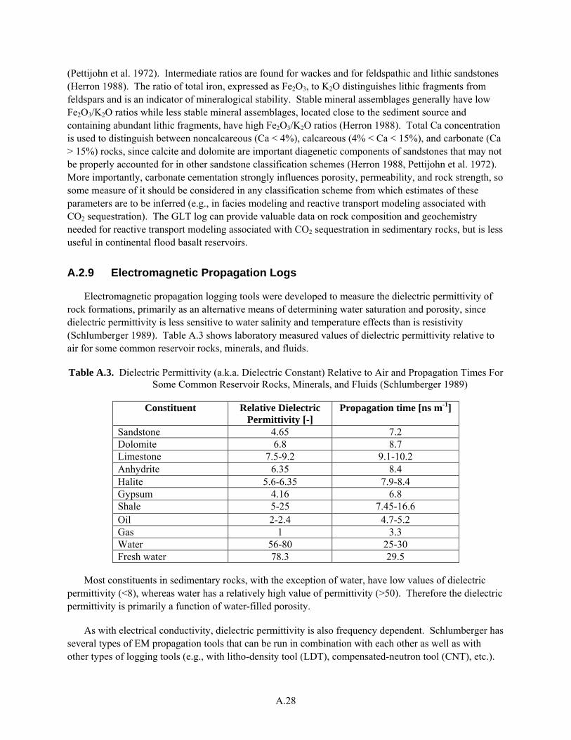
A.28

(Pettijohn et al. 1972). Intermediate ratios are found for wackes and for feldspathic and lithic sandstones (Herron 1988). The ratio of total iron, expressed as Fe2O3, to K2O distinguishes lithic fragments from feldspars and is an indicator of mineralogical stability. Stable mineral assemblages generally have low Fe2O3/K2O ratios while less stable mineral assemblages, located close to the sediment source and containing abundant lithic fragments, have high Fe2O3/K2O ratios (Herron 1988). Total Ca concentration is used to distinguish between noncalcareous (Ca < 4%), calcareous (4% < Ca < 15%), and carbonate (Ca > 15%) rocks, since calcite and dolomite are important diagenetic components of sandstones that may not be properly accounted for in other sandstone classification schemes (Herron 1988, Pettijohn et al. 1972). More importantly, carbonate cementation strongly influences porosity, permeability, and rock strength, so some measure of it should be considered in any classification scheme from which estimates of these parameters are to be inferred (e.g., in facies modeling and reactive transport modeling associated with CO2 sequestration). The GLT log can provide valuable data on rock composition and geochemistry needed for reactive transport modeling associated with CO2 sequestration in sedimentary rocks, but is less useful in continental flood basalt reservoirs.

A.2.9 Electromagnetic Propagation Logs

Electromagnetic propagation logging tools were developed to measure the dielectric permittivity of rock formations, primarily as an alternative means of determining water saturation and porosity, since dielectric permittivity is less sensitive to water salinity and temperature effects than is resistivity (Schlumberger 1989). Table A.3 shows laboratory measured values of dielectric permittivity relative to air for some common reservoir rocks, minerals, and fluids.

Table A.3. Dielectric Permittivity (a.k.a. Dielectric Constant) Relative to Air and Propagation Times For Some Common Reservoir Rocks, Minerals, and Fluids (Schlumberger 1989)

Constituent Relative Dielectric Permittivity [-]

Propagation time [ns m-1]

Sandstone 4.65 7.2 Dolomite 6.8 8.7 Limestone 7.5-9.2 9.1-10.2 Anhydrite 6.35 8.4 Halite 5.6-6.35 7.9-8.4 Gypsum 4.16 6.8 Shale 5-25 7.45-16.6 Oil 2-2.4 4.7-5.2 Gas 1 3.3 Water 56-80 25-30 Fresh water 78.3 29.5

Most constituents in sedimentary rocks, with the exception of water, have low values of dielectric permittivity (<8), whereas water has a relatively high value of permittivity (>50). Therefore the dielectric permittivity is primarily a function of water-filled porosity.

As with electrical conductivity, dielectric permittivity is also frequency dependent. Schlumberger has several types of EM propagation tools that can be run in combination with each other as well as with other types of logging tools (e.g., with litho-density tool (LDT), compensated-neutron tool (CNT), etc.).

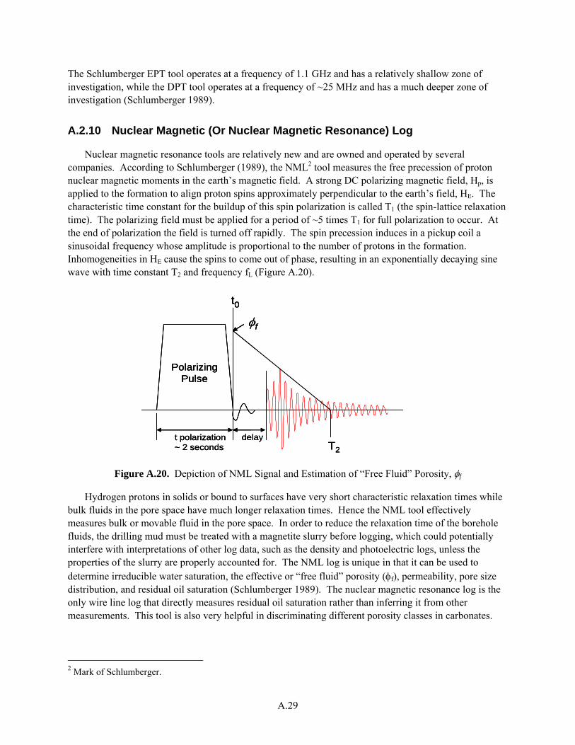
A.29

The Schlumberger EPT tool operates at a frequency of 1.1 GHz and has a relatively shallow zone of investigation, while the DPT tool operates at a frequency of ~25 MHz and has a much deeper zone of investigation (Schlumberger 1989).

A.2.10 Nuclear Magnetic (Or Nuclear Magnetic Resonance) Log

Nuclear magnetic resonance tools are relatively new and are owned and operated by several companies. According to Schlumberger (1989), the NML2 tool measures the free precession of proton nuclear magnetic moments in the earth’s magnetic field. A strong DC polarizing magnetic field, Hp, is applied to the formation to align proton spins approximately perpendicular to the earth’s field, HE. The characteristic time constant for the buildup of this spin polarization is called T1 (the spin-lattice relaxation time). The polarizing field must be applied for a period of ~5 times T1 for full polarization to occur. At the end of polarization the field is turned off rapidly. The spin precession induces in a pickup coil a sinusoidal frequency whose amplitude is proportional to the number of protons in the formation. Inhomogeneities in HE cause the spins to come out of phase, resulting in an exponentially decaying sine wave with time constant T2 and frequency fL (Figure A.20).

t polarization~ 2 seconds T2

t0

delay

φf

PolarizingPulse

t polarization~ 2 seconds T2

t0

delay

φf

PolarizingPulse

t polarization~ 2 seconds T2

t0

delay

φf

PolarizingPulse

Figure A.20. Depiction of NML Signal and Estimation of “Free Fluid” Porosity, φf

Hydrogen protons in solids or bound to surfaces have very short characteristic relaxation times while bulk fluids in the pore space have much longer relaxation times. Hence the NML tool effectively measures bulk or movable fluid in the pore space. In order to reduce the relaxation time of the borehole fluids, the drilling mud must be treated with a magnetite slurry before logging, which could potentially interfere with interpretations of other log data, such as the density and photoelectric logs, unless the properties of the slurry are properly accounted for. The NML log is unique in that it can be used to determine irreducible water saturation, the effective or “free fluid” porosity (φf), permeability, pore size distribution, and residual oil saturation (Schlumberger 1989). The nuclear magnetic resonance log is the only wire line log that directly measures residual oil saturation rather than inferring it from other measurements. This tool is also very helpful in discriminating different porosity classes in carbonates.

2 Mark of Schlumberger.

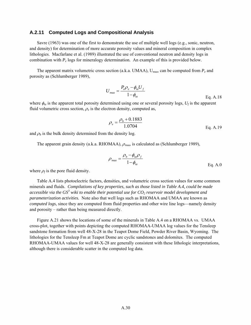
A.30

A.2.11 Computed Logs and Compositional Analysis

Savre (1963) was one of the first to demonstrate the use of multiple well logs (e.g., sonic, neutron, and density) for determination of more accurate porosity values and mineral composition in complex lithologies. Macfarlane et al. (1989) illustrated the use of conventional neutron and density logs in combination with Pe logs for mineralogy determination. An example of this is provided below.

The apparent matrix volumetric cross section (a.k.a. UMAA), Umaa, can be computed from Pe and porosity as (Schlumberger 1989),

ta

ftaeemaa

UPU

φφρ

−−

=1 Eq. A.18

where φta is the apparent total porosity determined using one or several porosity logs, Uf is the apparent fluid volumetric cross section, ρe is the electron density, computed as,

0704.11883.0+

= be

ρρ Eq. A.19

and ρb is the bulk density determined from the density log.

The apparent grain density (a.k.a. RHOMAA), ρmaa, is calculated as (Schlumberger 1989),

ta

ftabmaa φ

ρφρρ

−−

=1 Eq. A.0

where ρf is the pore fluid density.

Table A.4 lists photoelectric factors, densities, and volumetric cross section values for some common minerals and fluids. Compilations of key properties, such as those listed in Table A.4, could be made accessible via the GS3 wiki to enable their potential use for CO2 reservoir model development and parameterization activities. Note also that well logs such as RHOMAA and UMAA are known as computed logs, since they are computed from fluid properties and other wire line logs—namely density and porosity – rather than being measured directly.

Figure A.21 shows the locations of some of the minerals in Table A.4 on a RHOMAA vs. UMAA cross-plot, together with points depicting the computed RHOMAA-UMAA log values for the Tensleep sandstone formation from well 48-X-28 in the Teapot Dome Field, Powder River Basin, Wyoming. The lithologies for the Tensleep Fm at Teapot Dome are cyclic sandstones and dolomites. The computed RHOMAA-UMAA values for well 48-X-28 are generally consistent with these lithologic interpretations, although there is considerable scatter in the computed log data.

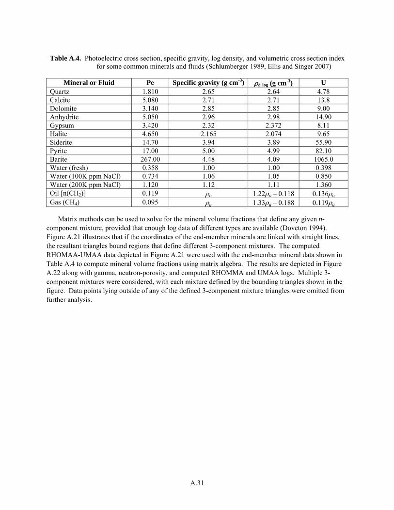
A.31

Table A.4. Photoelectric cross section, specific gravity, log density, and volumetric cross section index for some common minerals and fluids (Schlumberger 1989, Ellis and Singer 2007)

Mineral or Fluid Pe Specific gravity (g cm-3) ρb log (g cm-3) U Quartz 1.810 2.65 2.64 4.78 Calcite 5.080 2.71 2.71 13.8 Dolomite 3.140 2.85 2.85 9.00 Anhydrite 5.050 2.96 2.98 14.90 Gypsum 3.420 2.32 2.372 8.11 Halite 4.650 2.165 2.074 9.65 Siderite 14.70 3.94 3.89 55.90 Pyrite 17.00 5.00 4.99 82.10 Barite 267.00 4.48 4.09 1065.0 Water (fresh) 0.358 1.00 1.00 0.398 Water (100K ppm NaCl) 0.734 1.06 1.05 0.850 Water (200K ppm NaCl) 1.120 1.12 1.11 1.360 Oil [n(CH2)] 0.119 ρo 1.22ρo – 0.118 0.136ρo Gas (CH4) 0.095 ρg 1.33ρg – 0.188 0.119ρg

Matrix methods can be used to solve for the mineral volume fractions that define any given n-component mixture, provided that enough log data of different types are available (Doveton 1994). Figure A.21 illustrates that if the coordinates of the end-member minerals are linked with straight lines, the resultant triangles bound regions that define different 3-component mixtures. The computed RHOMAA-UMAA data depicted in Figure A.21 were used with the end-member mineral data shown in Table A.4 to compute mineral volume fractions using matrix algebra. The results are depicted in Figure A.22 along with gamma, neutron-porosity, and computed RHOMMA and UMAA logs. Multiple 3-component mixtures were considered, with each mixture defined by the bounding triangles shown in the figure. Data points lying outside of any of the defined 3-component mixture triangles were omitted from further analysis.

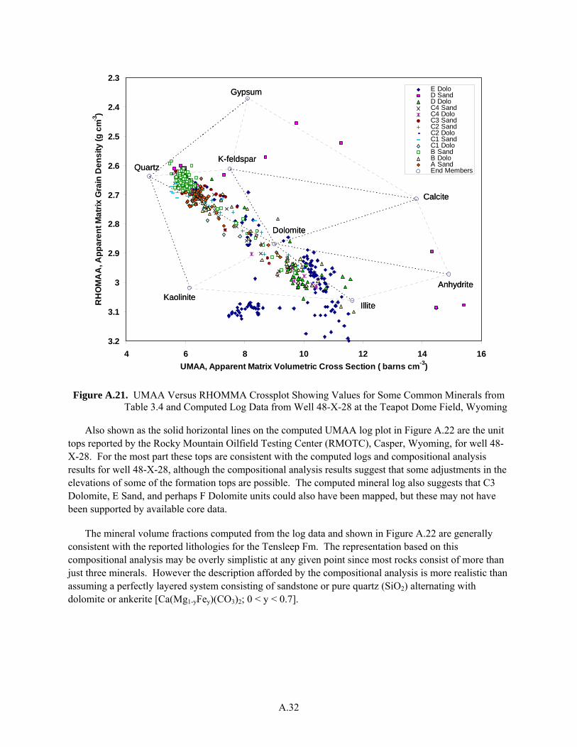
A.32

2.3

2.4

2.5

2.6

2.7

2.8

2.9

3

3.1

3.24 6 8 10 12 14 16

UMAA, Apparent Matrix Volumetric Cross Section ( barns cm-3)

RH

OM

AA

, App

aren

t Mat

rix G

rain

Den

sity

(g c

m-3)

E DoloD SandD DoloC4 SandC4 DoloC3 SandC2 SandC2 DoloC1 SandC1 DoloB SandB DoloA SandEnd MembersQuartz

K-feldspar

Gypsum

Calcite

AnhydriteKaolinite

Dolomite

Illite

2.3

2.4

2.5

2.6

2.7

2.8

2.9

3

3.1

3.24 6 8 10 12 14 16

UMAA, Apparent Matrix Volumetric Cross Section ( barns cm-3)

RH

OM

AA

, App

aren

t Mat

rix G

rain

Den

sity

(g c

m-3)

E DoloD SandD DoloC4 SandC4 DoloC3 SandC2 SandC2 DoloC1 SandC1 DoloB SandB DoloA SandEnd MembersQuartz

K-feldspar

Gypsum

Calcite

AnhydriteKaolinite

Dolomite

Illite

QuartzK-feldspar

Gypsum

Calcite

AnhydriteKaolinite

Dolomite

Illite

Figure A.21. UMAA Versus RHOMMA Crossplot Showing Values for Some Common Minerals from Table 3.4 and Computed Log Data from Well 48-X-28 at the Teapot Dome Field, Wyoming

Also shown as the solid horizontal lines on the computed UMAA log plot in Figure A.22 are the unit tops reported by the Rocky Mountain Oilfield Testing Center (RMOTC), Casper, Wyoming, for well 48-X-28. For the most part these tops are consistent with the computed logs and compositional analysis results for well 48-X-28, although the compositional analysis results suggest that some adjustments in the elevations of some of the formation tops are possible. The computed mineral log also suggests that C3 Dolomite, E Sand, and perhaps F Dolomite units could also have been mapped, but these may not have been supported by available core data.

The mineral volume fractions computed from the log data and shown in Figure A.22 are generally consistent with the reported lithologies for the Tensleep Fm. The representation based on this compositional analysis may be overly simplistic at any given point since most rocks consist of more than just three minerals. However the description afforded by the compositional analysis is more realistic than assuming a perfectly layered system consisting of sandstone or pure quartz (SiO2) alternating with dolomite or ankerite [Ca(Mg1-yFey)(CO3)2; 0 < y < 0.7].

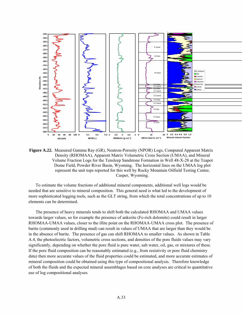
A.33

0 0.1 0.2 0.3NPOR (-)

2 2.5 3 3.5 4RHOMAA (g cm-3)

0 10 20UMAA (barns cm-3)

0 0.2 0.4 0.6 0.8 1

3

3

3

3

3

3

3

3

3

3

3

3

3

3

3

3

3

3

3

3

3

3

3

3

3

3

Mineral volume fraction

0 0.2 0.4 0.6 0.8 1.0

K-feldsparIlliteKaoliniteGypsumAnhydriteDolomiteCalciteQuartz

Mineral volume fraction

A Sand

B Dolo

B Sand

C1 DoloC1 SandC2 DoloC2 Sand

C3 Sand

C4 Dolo

C4 Sand

D Dolo

D Sand

E Dolo

-583

-573

-563

-553

-543

-533

-523

-513

-503

-493

-483

-473

-463

-453

-443

-433

-423

-413

-403

-393

-383

-373

-363

-353

-343

-333

0 20 40 60 80 100

GR (API)

Elev

atio

n (f

t)

0 0.1 0.2 0.3NPOR (-)

2 2.5 3 3.5 4RHOMAA (g cm-3)

0 10 20UMAA (barns cm-3)

0 0.2 0.4 0.6 0.8 1

3

3

3

3

3

3

3

3

3

3

3

3

3

3

3

3

3

3

3

3

3

3

3

3

3

3

Mineral volume fraction

0 0.2 0.4 0.6 0.8 1.0

K-feldsparIlliteKaoliniteGypsumAnhydriteDolomiteCalciteQuartz

Mineral volume fraction

A Sand

B Dolo

B Sand

C1 DoloC1 SandC2 DoloC2 Sand

C3 Sand

C4 Dolo

C4 Sand

D Dolo

D Sand

E Dolo

-583

-573

-563

-553

-543

-533

-523

-513

-503

-493

-483

-473

-463

-453

-443

-433

-423

-413

-403

-393

-383

-373

-363

-353

-343

-333

0 20 40 60 80 100

GR (API)

Elev

atio

n (f

t)

Figure A.22. Measured Gamma Ray (GR), Neutron-Porosity (NPOR) Logs, Computed Apparent Matrix Density (RHOMAA), Apparent Matrix Volumetric Cross Section (UMAA), and Mineral

Volume Fraction Logs for the Tensleep Sandstone Formation in Well 48-X-28 at the Teapot Dome Field, Powder River Basin, Wyoming. The horizontal lines on the UMAA log plot represent the unit tops reported for this well by Rocky Mountain Oilfield Testing Center,

Casper, Wyoming.

To estimate the volume fractions of additional mineral components, additional well logs would be needed that are sensitive to mineral composition. This general need is what led to the development of more sophisticated logging tools, such as the GLT string, from which the total concentrations of up to 10 elements can be determined.

The presence of heavy minerals tends to shift both the calculated RHOMAA and UMAA values towards larger values, so for example the presence of ankerite (Fe-rich dolomite) could result in larger RHOMAA-UMAA values, closer to the illite point on the RHOMAA-UMAA cross plot. The presence of barite (commonly used in drilling mud) can result in values of UMAA that are larger than they would be in the absence of barite. The presence of gas can shift RHOMAA to smaller values. As shown in Table A.4, the photoelectric factors, volumetric cross sections, and densities of the pore fluids values may vary significantly, depending on whether the pore fluid is pure water, salt water, oil, gas, or mixtures of these. If the pore fluid composition can be reasonably estimated (e.g., from resistivity or pore fluid chemistry data) then more accurate values of the fluid properties could be estimated, and more accurate estimates of mineral composition could be obtained using this type of compositional analysis. Therefore knowledge of both the fluids and the expected mineral assemblages based on core analyses are critical to quantitative use of log compositional analyses.

A.34

The system of equations used for estimating the volume fractions of three mineral components from two computed logs, as depicted in Figures A.21 and A.22, is fully determined, meaning that only one possible solution exists for each UMAA-RHOMAA point lying within a given 3-component mixture triangle. This type of analysis can be extended to n-component mixtures given (n - 1) logs that are sensitive to the properties being estimated. Doveton (1994) describes other solution methods for both underdetermined and overdetermined systems of equations that can be developed for rock compositional analysis. One such method for overdetermined systems is known as singular value decomposition, or SVD. Some commercial software packages for petrophysical analysis also use SVD (e.g., Interactive Petrophysics™ software by Schlumberger, see Appendix B). Generalized optimization approaches account for various user-defined constraints and logging tool error functions (Mayer and Sibbit 1980, Gysen et al. 1987).

Mineral volume fractions determined by compositional analyses with computed logs, such as RHOMAA and UMAA, or elemental mass fractions from geochemical logs obtained using the GLT, may be used as input for geochemical reactive transport modeling in CO2 sequestration studies, but care must be taken to ensure that logs from different wells are comparable, corrected for environmental effects and drilling fluids, and use common calibration standards (e.g., American Petroleum Institute). Many of the types of wire line log data noted above are not typically available in groundwater studies and they are therefore generally not used for hydrologic applications of reactive transport modeling. More typically, in hydrologic applications aqueous chemistry data are used in conjunction with thermodynamic databases of equilibrium aqueous-speciation and solid-phase (precipitation-dissolution) reactions with solubility product constants to determine saturation indices of various minerals. Minerals that are calculated to be supersaturated are plausible candidates for consideration as solid-phase components in geochemical reaction networks that are used to describe the groundwater system. If the minerals that are calculated to be supersaturated have also been observed in core samples or drill cuttings from the field, then they are usually accepted as solid-phase components of the system. A subset of all possible minerals and aqueous components is usually selected to define the geochemical reaction network based on core observations, computed saturation indices, and on the aqueous species with the highest activities or concentrations (e.g., >10-9 M).

If mineral volume fractions could be estimated independently from analysis of wire line log data, then thermodynamic databases could also be used with these data to estimate corresponding aqueous species concentrations. Ideally, the results from geochemical equilibrium calculations based primarily on aqueous chemistry data would be consistent with those that are based primarily on estimates of solid-phase mineralogical composition determined using log and core data. Discrepancies are likely, however, owing to mixing of groundwater from zones of differing lithologies within the wellbore, versus the more discrete and spatially explicit results that would likely be obtained based on well log and core data. Discrepancies would also be expected owing to inaccuracies in the log data themselves, because of assumptions that may be made about the number and types of minerals that comprise the geologic system of interest and due to scale differences between sparse core- and more prevalent well-log based estimates of mineralogy. The point here is that in principal one could use aqueous chemistry data and thermodynamic databases to infer solid-phase composition, or else use core- and log-based estimates of solid-phase composition with thermodynamic databases to infer aqueous solution chemistry. If both were done, the two sets of results should be consistent, assuming that a common set of minerals was selected in both cases. Although mixing of groundwater would tend to smooth differences in aqueous chemistry, wireline conveyed fluid sampling is a standard technology that can vent produced fluids until there is

A.35

some assurance of production of true formation fluids. Further evaluation of this topic is warranted to determine the effects of using different data types (e.g., aqueous chemistry versus solid-phase mineral composition inferred from wire line log and core data) and assumptions about mineral composition on reactive transport associated with CO2 sequestration. This could be a valuable area of future research for PNNL.

A.2.12 Lithostratigraphic Correlation

One of the primary purposes of well log analysis is to determine so-called geologic or unit “picks” or “tops” which are the depths or elevations of the tops of major or distinctive stratigraphic units within a geologic profile. Geologic tops can be identified by evaluation of driller’s and geologic logs and by using measured or computed geophysical logs, such as those shown in Figure A.22, in conjunction with inspection of well cuttings and core samples to identify major interfaces between well-defined geologic units. Figure A.23 shows another example with depth-registered geologic picks for formation tops that can be an important component of reservoir model development. Such tops are commonly used as the basis for establishing correlations between different wells to determine the spatial continuity of units. Unit tops are also generally required for performing depth-to-time conversions that allow well log data and seismic data to be compared on an equal basis. Unit tops are also used in the development of computational grids or meshes to ensure that the locations of major stratigraphic interfaces within the system are accurately represented in numerical models used to simulate subsurface flow and transport. The process of defining unit tops and correlating well logs involves some manual steps but interative software programs that can greatly facilitate this process include Correlator (Olea 2004), developed by the Kansas Geological Survey, numerous PC-based programs, and Petrel™ and Interactive Petrophysics™, both marketed by Schlumberger.

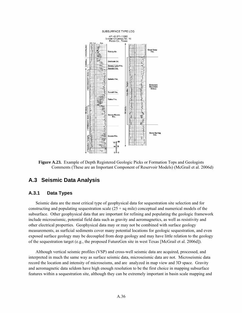
A.36

Figure A.23. Example of Depth Registered Geologic Picks or Formation Tops and Geologists Comments (These are an Important Component of Reservoir Models) (McGrail et al. 2006d)

A.3 Seismic Data Analysis

A.3.1 Data Types

Seismic data are the most critical type of geophysical data for sequestration site selection and for constructing and populating sequestration scale (25 + sq mile) conceptual and numerical models of the subsurface. Other geophysical data that are important for refining and populating the geologic framework include microseismic, potential field data such as gravity and aeromagnetics, as well as resistivity and other electrical properties. Geophysical data may or may not be combined with surface geology measurements, as surficial sediments cover many potential locations for geologic sequestration, and even exposed surface geology may be decoupled from deep geology and may have little relation to the geology of the sequestration target (e.g., the proposed FutureGen site in west Texas [McGrail et al. 2006d]).

Although vertical seismic profiles (VSP) and cross-well seismic data are acquired, processed, and interpreted in much the same way as surface seismic data, microseismic data are not. Microseismic data record the location and intensity of microseisms, and are analyzed in map view and 3D space. Gravity and aeromagnetic data seldom have high enough resolution to be the first choice in mapping subsurface features within a sequestration site, although they can be extremely important in basin scale mapping and

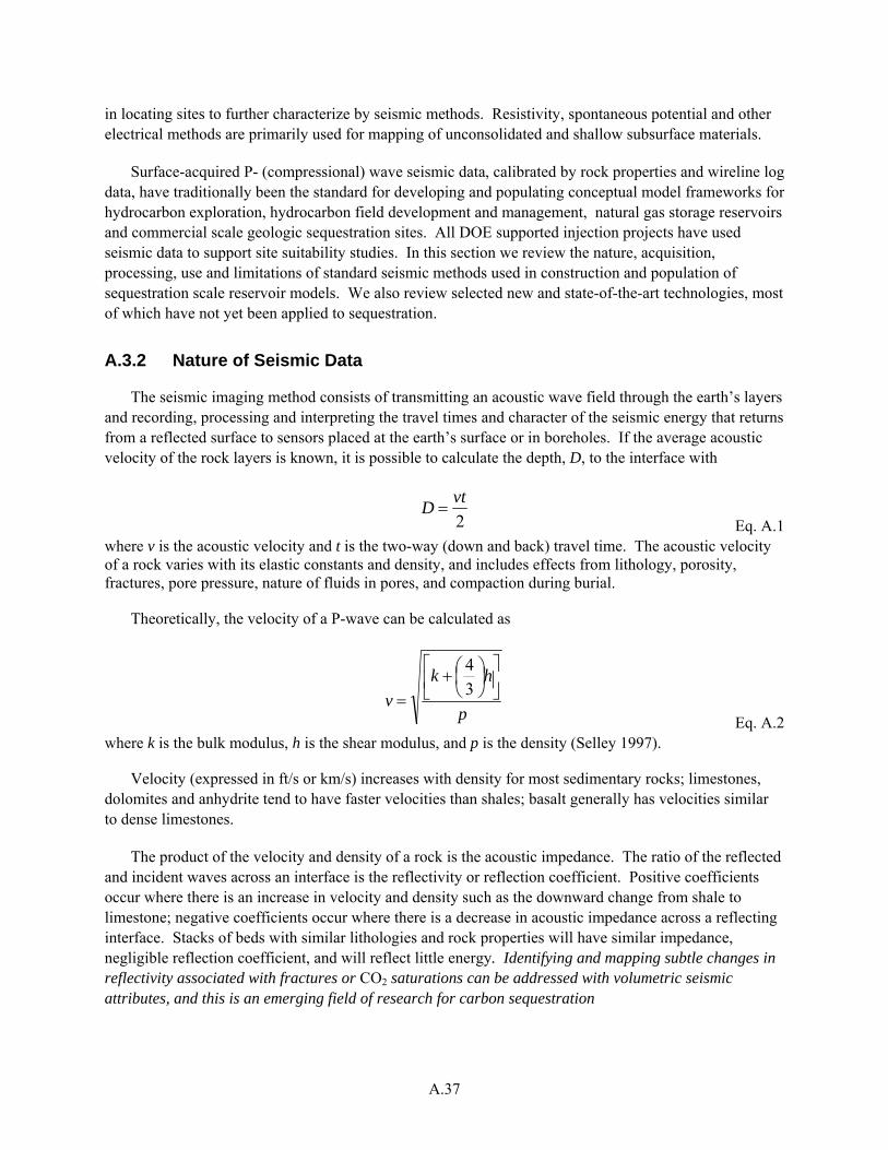
A.37

in locating sites to further characterize by seismic methods. Resistivity, spontaneous potential and other electrical methods are primarily used for mapping of unconsolidated and shallow subsurface materials.

Surface-acquired P- (compressional) wave seismic data, calibrated by rock properties and wireline log data, have traditionally been the standard for developing and populating conceptual model frameworks for hydrocarbon exploration, hydrocarbon field development and management, natural gas storage reservoirs and commercial scale geologic sequestration sites. All DOE supported injection projects have used seismic data to support site suitability studies. In this section we review the nature, acquisition, processing, use and limitations of standard seismic methods used in construction and population of sequestration scale reservoir models. We also review selected new and state-of-the-art technologies, most of which have not yet been applied to sequestration.

A.3.2 Nature of Seismic Data

The seismic imaging method consists of transmitting an acoustic wave field through the earth’s layers and recording, processing and interpreting the travel times and character of the seismic energy that returns from a reflected surface to sensors placed at the earth’s surface or in boreholes. If the average acoustic velocity of the rock layers is known, it is possible to calculate the depth, D, to the interface with

2vtD =

Eq. A.1 where v is the acoustic velocity and t is the two-way (down and back) travel time. The acoustic velocity of a rock varies with its elastic constants and density, and includes effects from lithology, porosity, fractures, pore pressure, nature of fluids in pores, and compaction during burial.

Theoretically, the velocity of a P-wave can be calculated as

p

hkv

⎥⎦

⎤⎢⎣

⎡⎟⎠⎞

⎜⎝⎛+

=34

Eq. A.2 where k is the bulk modulus, h is the shear modulus, and p is the density (Selley 1997).

Velocity (expressed in ft/s or km/s) increases with density for most sedimentary rocks; limestones, dolomites and anhydrite tend to have faster velocities than shales; basalt generally has velocities similar to dense limestones.

The product of the velocity and density of a rock is the acoustic impedance. The ratio of the reflected and incident waves across an interface is the reflectivity or reflection coefficient. Positive coefficients occur where there is an increase in velocity and density such as the downward change from shale to limestone; negative coefficients occur where there is a decrease in acoustic impedance across a reflecting interface. Stacks of beds with similar lithologies and rock properties will have similar impedance, negligible reflection coefficient, and will reflect little energy. Identifying and mapping subtle changes in reflectivity associated with fractures or CO2 saturations can be addressed with volumetric seismic attributes, and this is an emerging field of research for carbon sequestration

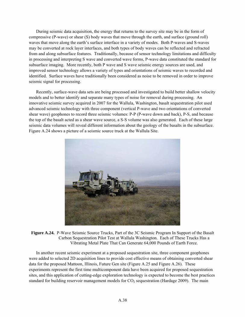
A.38

During seismic data acquisition, the energy that returns to the survey site may be in the form of compressive (P-wave) or shear (S) body waves that move through the earth, and surface (ground roll) waves that move along the earth’s surface interface in a variety of modes. Both P-waves and S-waves may be converted at rock layer interfaces, and both types of body waves can be reflected and refracted from and along subsurface features. Traditionally, because of sensor technology limitations and difficulty in processing and interpreting S wave and converted wave forms, P-wave data constituted the standard for subsurface imaging. More recently, both P wave and S wave seismic energy sources are used, and improved sensor technology allows a variety of types and orientations of seismic waves to recorded and identified. Surface waves have traditionally been considered as noise to be removed in order to improve seismic signal for processing.

Recently, surface-wave data sets are being processed and investigated to build better shallow velocity models and to better identify and separate many types of noise for removal during processing. An innovative seismic survey acquired in 2007 for the Wallula, Washington, basalt sequestration pilot used advanced seismic technology with three component (vertical P-wave and two orientations of converted shear wave) geophones to record three seismic volumes: P-P (P-wave down and back), P-S, and because the top of the basalt acted as a shear wave source, a S-S volume was also generated. Each of these large seismic data volumes will reveal different information about the geology of the basalts in the subsurface. Figure A.24 shows a picture of a seismic source truck at the Wallula Site.

Figure A.24. P-Wave Seismic Source Trucks, Part of the 3C Seismic Program In Support of the Basalt Carbon Sequestration Pilot Test at Wallula Washington. Each of These Trucks Has a

Vibrating Metal Plate That Can Generate 64,000 Pounds of Earth Force.

In another recent seismic experiment at a proposed sequestration site, three component geophones were added to selected 2D acquisition lines to provide cost effective means of obtaining converted shear data for the proposed Mattoon, Illinois, Future Gen site (Figure A.25 and Figure A.26). These experiments represent the first time multicomponent data have been acquired for proposed sequestration sites, and this application of cutting-edge exploration technology is expected to become the best practices standard for building reservoir management models for CO2 sequestration (Hardage 2009). The main

A.39

consequence of this Battelle, Pacific Northwest Division-led technology trend is the generation of multiple large seismic data volumes for each site that contain greater potential for imaging subtle geologic features and for identifying and mapping spatial and temporal changes in rock, fluid and geomechanical properties. The assimilation of large volumes of seismic data with other data types is one of the largest challenges and greatest opportunities for innovation in improving conceptual and numerical models for carbon sequestration.

Figure A.25. Wiggle-Trace Display of P-Wave 2D Seismic Data from the Recently Re-started Futuregen Sequestration Project at Mattoon, Illinois. Dark Events Represent Velocity Contrasts

Associated With Changes in Rock, Fluid, Pressure, or Geomechanical Properties.

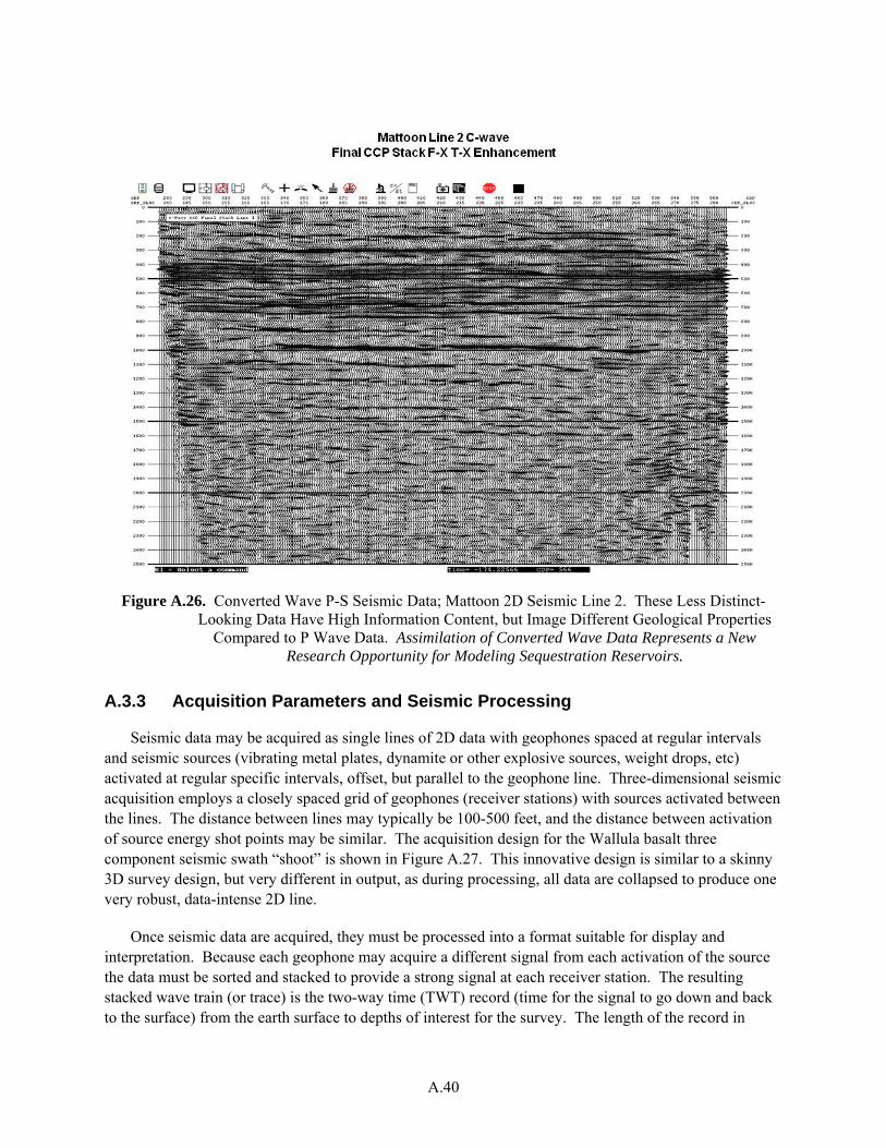
A.40

Figure A.26. Converted Wave P-S Seismic Data; Mattoon 2D Seismic Line 2. These Less Distinct-Looking Data Have High Information Content, but Image Different Geological Properties

Compared to P Wave Data. Assimilation of Converted Wave Data Represents a New Research Opportunity for Modeling Sequestration Reservoirs.

A.3.3 Acquisition Parameters and Seismic Processing

Seismic data may be acquired as single lines of 2D data with geophones spaced at regular intervals and seismic sources (vibrating metal plates, dynamite or other explosive sources, weight drops, etc) activated at regular specific intervals, offset, but parallel to the geophone line. Three-dimensional seismic acquisition employs a closely spaced grid of geophones (receiver stations) with sources activated between the lines. The distance between lines may typically be 100-500 feet, and the distance between activation of source energy shot points may be similar. The acquisition design for the Wallula basalt three component seismic swath “shoot” is shown in Figure A.27. This innovative design is similar to a skinny 3D survey design, but very different in output, as during processing, all data are collapsed to produce one very robust, data-intense 2D line.

Once seismic data are acquired, they must be processed into a format suitable for display and interpretation. Because each geophone may acquire a different signal from each activation of the source the data must be sorted and stacked to provide a strong signal at each receiver station. The resulting stacked wave train (or trace) is the two-way time (TWT) record (time for the signal to go down and back to the surface) from the earth surface to depths of interest for the survey. The length of the record in

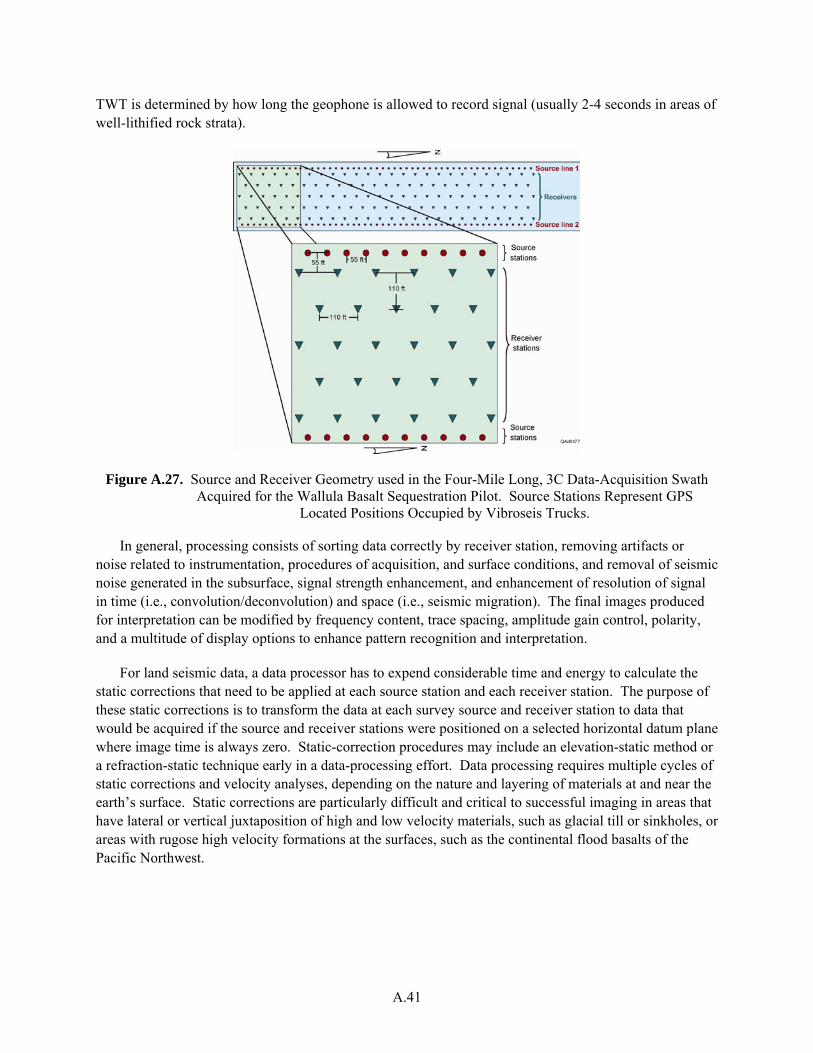
A.41

TWT is determined by how long the geophone is allowed to record signal (usually 2-4 seconds in areas of well-lithified rock strata).

Figure A.27. Source and Receiver Geometry used in the Four-Mile Long, 3C Data-Acquisition Swath Acquired for the Wallula Basalt Sequestration Pilot. Source Stations Represent GPS

Located Positions Occupied by Vibroseis Trucks.

In general, processing consists of sorting data correctly by receiver station, removing artifacts or noise related to instrumentation, procedures of acquisition, and surface conditions, and removal of seismic noise generated in the subsurface, signal strength enhancement, and enhancement of resolution of signal in time (i.e., convolution/deconvolution) and space (i.e., seismic migration). The final images produced for interpretation can be modified by frequency content, trace spacing, amplitude gain control, polarity, and a multitude of display options to enhance pattern recognition and interpretation.

For land seismic data, a data processor has to expend considerable time and energy to calculate the static corrections that need to be applied at each source station and each receiver station. The purpose of these static corrections is to transform the data at each survey source and receiver station to data that would be acquired if the source and receiver stations were positioned on a selected horizontal datum plane where image time is always zero. Static-correction procedures may include an elevation-static method or a refraction-static technique early in a data-processing effort. Data processing requires multiple cycles of static corrections and velocity analyses, depending on the nature and layering of materials at and near the earth’s surface. Static corrections are particularly difficult and critical to successful imaging in areas that have lateral or vertical juxtaposition of high and low velocity materials, such as glacial till or sinkholes, or areas with rugose high velocity formations at the surfaces, such as the continental flood basalts of the Pacific Northwest.

A.42

A.3.4 Vertical and Lateral Resolution of Seismic Data

Seismic resolution is the ability to distinguish between subsurface objects, or how far apart two interfaces must be to distinguish separate reflections from the objects. For example, interpreters are concerned with vertical resolution, e.g., how thick a bed must be before the top and bottom can be separately imaged. Interpreters are also concerned with lateral resolution- how narrow can a fracture zone be and still be reliably resolved. Fortunately in seismic data, many objects below resolution can still be detected.

In general the vertical resolution (or distinction) of two surfaces is about 1/4 of the acoustic wavelength. Since wavelength equals velocity divided by frequency, this would translate into a 25' resolution for a moderately shallow bed that has an acoustic velocity of 6,000 ft/sec and a seismic wavelet with 60Hz dominant frequency, or resolution of about 250 feet for a deep bed with a velocity of 15,000 ft/sec and 15Hz dominant frequency. This decrease in resolution with depth is due to two factors. Rock beds tend to increase in velocity with depth because of increased compaction and cementation (that leads to decreased porosity and increased density); in addition, the earth acts as a filter causing frequency to decrease with depth. This knowledge is taken into account in planning seismic acquisition. For example, field tests prior to seismic acquisition at Wallula indicated the maximum dominant frequency that we could expect at a depth of 4000' was about 80 Hz. Thus if seismic velocity in the basalt layers was 16,000 ft/sec, we could expect a wavelength of 200 ft, and resolution of a bed of one-fourth of that thickness, or 50 feet. With the use of seismic attributes, however, we expect to be able to detect vertical features that are 1/10 of a wavelength, or 20 feet. Crosswell seismic obtains much higher frequencies than surface seismic, and can obtain resolution of about three feet. This is important in model building, since fine scale resolution near a borehole allows calibration of lower resolution volumes of surface seismic data.

Horizontal resolution is more complex. The acoustic waves that produce an image of a surface are reflected from a fairly large circular area of that surface known as the Fresnel zone. Reflections from this area constructively interfere when they arrive at the geophone. The radius of this zone approximates horizontal resolution for unmigrated data; radii are commonly given as nomograms in seismic literature Sheriff 1980). For a 60 Hz wavelet at 5000 feet depth, and a rock velocity of 6000 ft/sec, lateral resolution is about 500 feet. With modern 3D seismic attributes, the detection limit is about 1/10 of the resolution; that is, we can expect to be able to image a fracture zone about 30-50 feet wide, although we cannot be precise about the exact location of the edge of the zone (Chopra and Marfurt 2005). Due to the same vertical changes that lead to decreases in vertical resolution, the radius of the Fresnel zone increases with depth, thus decreasing the horizontal resolution.

A.3.4.1 Depth Conversion

Depth migration may be conducted as part of seismic processing or as a post stack option in interpretation software packages such as Geoframe or the Kingdom Software Suite. To convert two-way time seismic data to depth, a velocity gradient cross-section or map is required for 2D data and a velocity field volume for 3D data. Depth conversion of a mapped time horizon involves multiplying a gridded one-way time map by a gridded velocity map constructed from wellbore measurements that establish points of known depth versus acoustic travel time (e.g., check shots and VSPs [vertical seismic profiles]). Velocities of layers of rock vary considerably both vertically and laterally, and depth converted horizons may have a very different structural configuration, compared to the original horizon mapped in the time domain.

A.43

A.3.4.2 Seismic Analysis Methods

Seismic data provide surfaces for definition of the framework for geologic models and seismic texture data that can be processed, calibrated, and interpreted to provide data for populating that structural framework. Seismic events (surfaces) provide robust data for mapping subsurface sequestration-scale, vertical and lateral bounding surfaces and geometries of formations, unconformities, faults, channels, reefs, fractures and other edges. Lateral and vertical changes in seismic texture or character are used to map seismic facies. These facies, when calibrated with wellbore and other data can be interpreted as lithofacies, diagenetic facies, 3D geobodies with distinct properties, gradual or sharp spatial changes in fluid saturations, pore pressure, porosity, permeability, grain size, rock strength, compressibility, or any of a number of rock physics properties that are important for constructing robust reservoir models. Surface seismic data may be acquired along 2D lines, or as 3D grids that produce a data volume. Wellbore seismic data, such as cross-well seismic and vertical seismic profiles (VSP) provide higher resolution 2D data between wellbores or between the wellbore and the earth's surface. Unless they are acquired as multiple lines, they do not produce data with lateral extent.

Both 2D lines and 2D extractions from a 3D volume can be displayed and analyzed in cross-section view. A conventional color display or visualization of one line of surface-acquired 2D P-wave seismic data from the proposed FutureGen site at Mattoon Illinois is shown in Figure A.28. These data were acquired as part of the same 2D survey lines shown in black and white, above. The data are displayed in variable density rather than in wiggle trace mode. Shot points are displayed along the top of the display, above the seismic. The display is in two way time, and the horizons have been correlated with the regional subsurface geology, based on assuming an average interval (rock) velocity of 15,000 feet/second, and on visual correlation with seismic character from well-bore calibrated seismic in other parts of the Illinois Basin. The 2D line images a series of almost horizontal layers of Paleozoic rock, unbroken by faults, above faulted Precambrian basement rock. The seismic character displays considerable lateral variation, related to changes in lithology, grain size, and perhaps fluid properties. This variation is the basis for subsequent mapping of seismic facies with a variety of 2D seismic attributes. These 2D data are insufficient for recent innovations in seismic facies mapping that require volumetric data.

A series of 2D seismic lines can be used to interpolate and map horizons, as well as outline faults, channels or other features that are intersected by the 2D lines, An interpreted structure map of the top of the Mount Simon reservoir at the Mattoon FutureGen site, converted from two way time to depth below ground surface is shown in Figure A.29. Shot points from the 2D seismic lines, from which the map was generated, are shown as small dots. Greater uncertainty is associated with the areas where the seismic line spacing is larger. These surfaces could serve as input into a numerical model building software package.

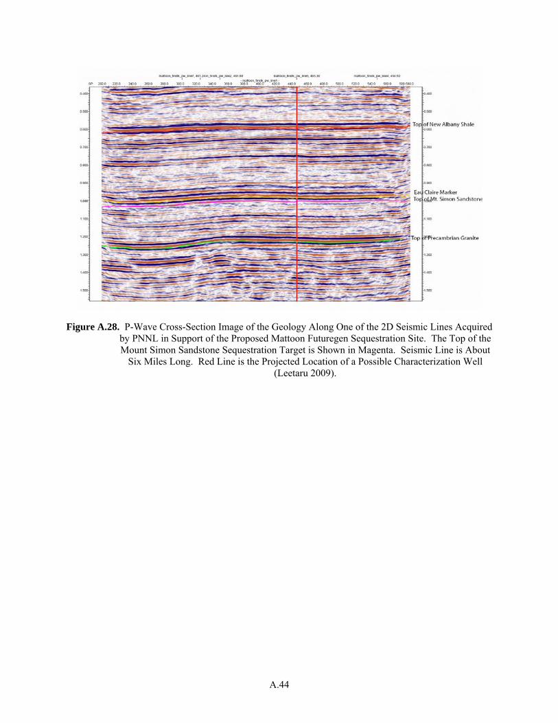
A.44

Figure A.28. P-Wave Cross-Section Image of the Geology Along One of the 2D Seismic Lines Acquired by PNNL in Support of the Proposed Mattoon Futuregen Sequestration Site. The Top of the Mount Simon Sandstone Sequestration Target is Shown in Magenta. Seismic Line is About

Six Miles Long. Red Line is the Projected Location of a Possible Characterization Well (Leetaru 2009).

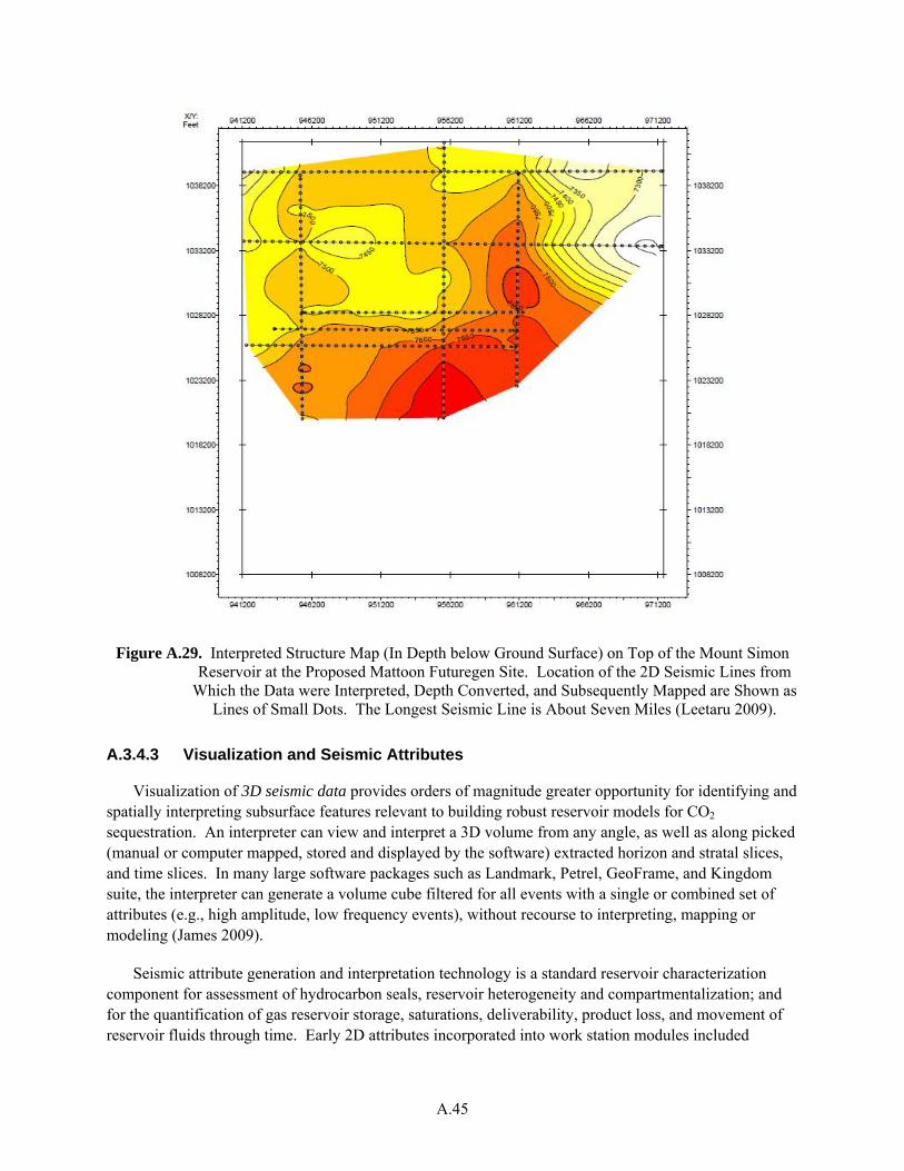
A.45

Figure A.29. Interpreted Structure Map (In Depth below Ground Surface) on Top of the Mount Simon Reservoir at the Proposed Mattoon Futuregen Site. Location of the 2D Seismic Lines from

Which the Data were Interpreted, Depth Converted, and Subsequently Mapped are Shown as Lines of Small Dots. The Longest Seismic Line is About Seven Miles (Leetaru 2009).

A.3.4.3 Visualization and Seismic Attributes

Visualization of 3D seismic data provides orders of magnitude greater opportunity for identifying and spatially interpreting subsurface features relevant to building robust reservoir models for CO2 sequestration. An interpreter can view and interpret a 3D volume from any angle, as well as along picked (manual or computer mapped, stored and displayed by the software) extracted horizon and stratal slices, and time slices. In many large software packages such as Landmark, Petrel, GeoFrame, and Kingdom suite, the interpreter can generate a volume cube filtered for all events with a single or combined set of attributes (e.g., high amplitude, low frequency events), without recourse to interpreting, mapping or modeling (James 2009).

Seismic attribute generation and interpretation technology is a standard reservoir characterization component for assessment of hydrocarbon seals, reservoir heterogeneity and compartmentalization; and for the quantification of gas reservoir storage, saturations, deliverability, product loss, and movement of reservoir fluids through time. Early 2D attributes incorporated into work station modules included

A.46

reflection strength, instantaneous phase and instantaneous frequency. Instantaneous phase is particularly helpful in identifying stratigraphic features. Attribute packages that are now on most workstation platforms involve analysis of wave shape, continuity, amplitude, phase, frequency and interval velocity. Many of these attributes address lateral variability and can be generated only along previously mapped seismic horizons (i.e., top of Mt Simon Sandstone). These attributes produce surfaces that can be depth converted, gridded and used as input in conceptual and numerical models. Other attributes address vertical changes and can be used to determine lateral extent of facies changes.

One of the most robust attributes is the generation of impedance inversion volumes. An example of the use of impedance inversion to image thin porous facies in a heterogeneous reservoir is given in Fu et al. (2006). In a study of Devonian turbidites in the subsurface of west Texas, Fu et al. (2006) integrated well logs, engineering data, and core-based fracture analysis and rock physics properties to improve the resolution of inter-well heterogeneity. They correlated the relations between porosity, velocity and permeability with 3D seismic attributes of impedance, coherence, and curvature. The overlay of one line of the original 3D seismic data with sonic well curves and the corresponding line from the impedance inversion volume is shown in Figure A.30. Original wiggle traces and well logs are in black; colored data are the inverted volume, which shows considerably more detail than the original wiggle trace data. The green color represents high impedance layers, yellow is lower impedance; the blue oval appears to outline a cross sectional view of a turbidite channel. Examination of additional vertical slices would permit 3D mapping of various features in the turbidite system and together with well log and core data, would form the basis for 3D depositional facies geobodies, which are valuable input for reservoir models, e.g., for the geostatistical mapping of lithofacies described in Section A.6.2.

Spectral decomposition is a standard tool for analyzing seismic attributes that unravels the seismic signal into its constituent frequencies. Intervals within a 3D volume are characterized by different frequencies, depending on stratigraphy and bed thickness, and fluid content. High frequencies image thin beds better, lower frequencies produce better images of features in thick beds. The interpreter can use amplitude and phase tuned to specific wavelengths to image subtle thickness variations and discontinuities, as well as (with rock physics calibration) view vertical changes and accurately predict bed thicknesses (Partyka et al. 1999, Castagna et al. 2003). Volume visualization and interpretation can further enhance the Spectral decomposition is a powerful technique that when combined with geometric attributes, can accelerate the interpretation of large seismic volumes and can greatly aid imaging and interpreting small-scale or subtle features in reservoir or caprock (Chopra and Marfurt 2007).

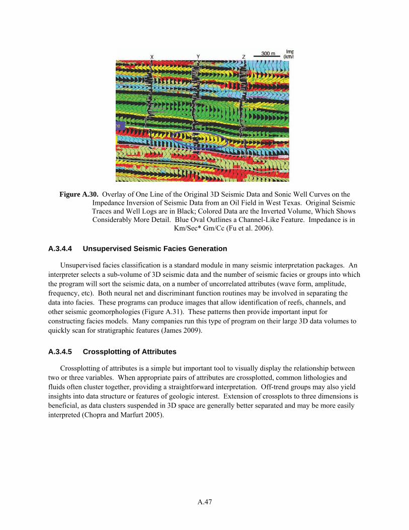
A.47

Figure A.30. Overlay of One Line of the Original 3D Seismic Data and Sonic Well Curves on the Impedance Inversion of Seismic Data from an Oil Field in West Texas. Original Seismic Traces and Well Logs are in Black; Colored Data are the Inverted Volume, Which Shows Considerably More Detail. Blue Oval Outlines a Channel-Like Feature. Impedance is in

Km/Sec* Gm/Cc (Fu et al. 2006).

A.3.4.4 Unsupervised Seismic Facies Generation

Unsupervised facies classification is a standard module in many seismic interpretation packages. An interpreter selects a sub-volume of 3D seismic data and the number of seismic facies or groups into which the program will sort the seismic data, on a number of uncorrelated attributes (wave form, amplitude, frequency, etc). Both neural net and discriminant function routines may be involved in separating the data into facies. These programs can produce images that allow identification of reefs, channels, and other seismic geomorphologies (Figure A.31). These patterns then provide important input for constructing facies models. Many companies run this type of program on their large 3D data volumes to quickly scan for stratigraphic features (James 2009).

A.3.4.5 Crossplotting of Attributes

Crossplotting of attributes is a simple but important tool to visually display the relationship between two or three variables. When appropriate pairs of attributes are crossplotted, common lithologies and fluids often cluster together, providing a straightforward interpretation. Off-trend groups may also yield insights into data structure or features of geologic interest. Extension of crossplots to three dimensions is beneficial, as data clusters suspended in 3D space are generally better separated and may be more easily interpreted (Chopra and Marfurt 2005).

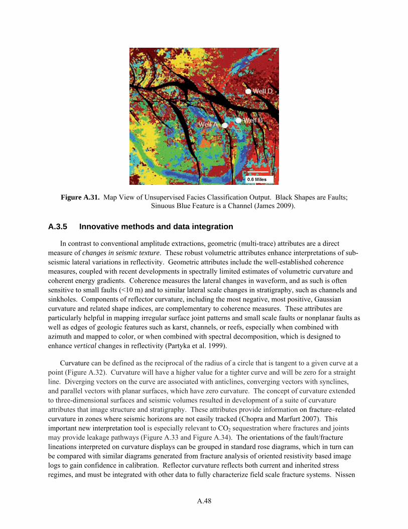
A.48

Figure A.31. Map View of Unsupervised Facies Classification Output. Black Shapes are Faults; Sinuous Blue Feature is a Channel (James 2009).

A.3.5 Innovative methods and data integration

In contrast to conventional amplitude extractions, geometric (multi-trace) attributes are a direct measure of changes in seismic texture. These robust volumetric attributes enhance interpretations of sub-seismic lateral variations in reflectivity. Geometric attributes include the well-established coherence measures, coupled with recent developments in spectrally limited estimates of volumetric curvature and coherent energy gradients. Coherence measures the lateral changes in waveform, and as such is often sensitive to small faults (<10 m) and to similar lateral scale changes in stratigraphy, such as channels and sinkholes. Components of reflector curvature, including the most negative, most positive, Gaussian curvature and related shape indices, are complementary to coherence measures. These attributes are particularly helpful in mapping irregular surface joint patterns and small scale faults or nonplanar faults as well as edges of geologic features such as karst, channels, or reefs, especially when combined with azimuth and mapped to color, or when combined with spectral decomposition, which is designed to enhance vertical changes in reflectivity (Partyka et al. 1999).

Curvature can be defined as the reciprocal of the radius of a circle that is tangent to a given curve at a point (Figure A.32). Curvature will have a higher value for a tighter curve and will be zero for a straight line. Diverging vectors on the curve are associated with anticlines, converging vectors with synclines, and parallel vectors with planar surfaces, which have zero curvature. The concept of curvature extended to three-dimensional surfaces and seismic volumes resulted in development of a suite of curvature attributes that image structure and stratigraphy. These attributes provide information on fracture–related curvature in zones where seismic horizons are not easily tracked (Chopra and Marfurt 2007). This important new interpretation tool is especially relevant to CO2 sequestration where fractures and joints may provide leakage pathways (Figure A.33 and Figure A.34). The orientations of the fault/fracture lineations interpreted on curvature displays can be grouped in standard rose diagrams, which in turn can be compared with similar diagrams generated from fracture analysis of oriented resistivity based image logs to gain confidence in calibration. Reflector curvature reflects both current and inherited stress regimes, and must be integrated with other data to fully characterize field scale fracture systems. Nissen

A.49

et al. (2007) in a study of a potential CO2 sequestration reservoir in Kansas, used water production data to determine which curvature based lineaments imaged open fractures.

These attributes have the potential to image features related to fractures and non-sealing faults that may compromise seal integrity of CO2 storage reservoirs, but which cannot be detected with other methods. In addition, volume-based estimates are of particular value for interpreting features in low signal-to-noise reservoir heterogeneity

Figure A.32. Curvature in Two Dimensions. Curvature is Defined as the Inverse of the Radius of a Circle that is Tangent to a Surface at any Point. By Convention, Positive Curvature is Convex Upward; Negative Curvature is Convex Downward. Anticlines Have Positive

Curvature; Synclines Have Negative Curvature (Blumentritt et al. 2006).

Figure A.33. Map-View Time Slice through a Fort Worth Basin 3D Mean Curvature Seismic Attribute Volume at 1.18 S., Near the Top of the Ordovician Ellenburger Formation. Note the Crisp

Imaging of the Subcircular Sinkhole Collapse Features. Scale Bar is Five Kilometers. (Sullivan et al. 2005)

5

1180 ms M

N

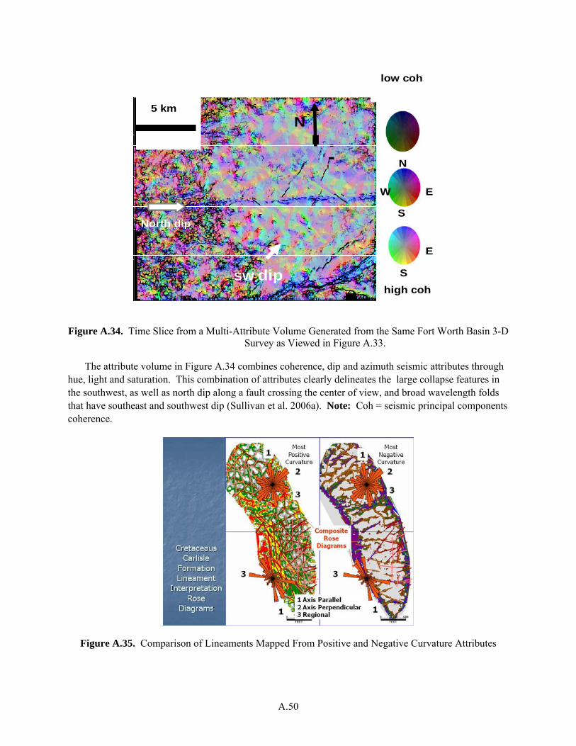
A.50

SW dip

North dip

5 km

N

E

S

E W

S

low coh

high coh

N

Figure A.34. Time Slice from a Multi-Attribute Volume Generated from the Same Fort Worth Basin 3-D Survey as Viewed in Figure A.33.

The attribute volume in Figure A.34 combines coherence, dip and azimuth seismic attributes through hue, light and saturation. This combination of attributes clearly delineates the large collapse features in the southwest, as well as north dip along a fault crossing the center of view, and broad wavelength folds that have southeast and southwest dip (Sullivan et al. 2006a). Note: Coh = seismic principal components coherence.

Figure A.35. Comparison of Lineaments Mapped From Positive and Negative Curvature Attributes

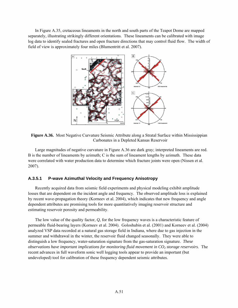
A.51

In Figure A.35, cretaceous lineaments in the north and south parts of the Teapot Dome are mapped separately, illustrating strikingly different orientations. These lineaments can be calibrated with image log data to identify sealed fractures and open fracture directions that may control fluid flow. The width of field of view is approximately four miles (Blumentritt et al. 2007).

Figure A.36. Most Negative Curvature Seismic Attribute along a Stratal Surface within Mississippian Carbonates in a Depleted Kansas Reservoir

Large magnitudes of negative curvature in Figure A.36 are dark gray; interpreted lineaments are red. B is the number of lineaments by azimuth; C is the sum of lineament lengths by azimuth. These data were correlated with water production data to determine which fracture joints were open (Nissen et al. 2007).

A.3.5.1 P-wave Azimuthal Velocity and Frequency Anisotropy

Recently acquired data from seismic field experiments and physical modeling exhibit amplitude losses that are dependent on the incident angle and frequency. The observed amplitude loss is explained by recent wave-propagation theory (Korneev et al. 2004), which indicates that new frequency and angle dependent attributes are promising tools for more quantitatively imaging reservoir structure and estimating reservoir porosity and permeability.

The low value of the quality factor, Q, for the low frequency waves is a characteristic feature of permeable fluid-bearing layers (Korneev et al. 2004). Goloshubin et al. (2001) and Korneev et al. (2004) analyzed VSP data recorded at a natural gas storage field in Indiana, where due to gas injection in the summer and withdrawal in the winter, the reservoir fluid changed seasonally. They were able to distinguish a low frequency, water-saturation signature from the gas-saturation signature. These observations have important implications for monitoring fluid movement in CO2 storage reservoirs. The recent advances in full waveform sonic well logging tools appear to provide an important (but undeveloped) tool for calibration of these frequency dependent seismic attributes.

A.52

A.3.5.2 Converted P-S Wave and S-S Wave Data

P and S seismic modes image different aspects of geology at depth-equivalent intervals, and are increasingly utilized in hydrocarbon exploration and development to differentiate sand versus shale, define bed specific fracture orientations, and map 3D seismic facies and geobodies. An example of differences in P-P and P-S images are shown for a West Texas carbonate field in Figure A.37. Because converted P-S and S-S waves travel more slowly through rocks that P-wave energy, and because S-waves travel only through rock and not through fluids, differences in travel time are used to detect azimuth of fluid filled fractures and joints. One of the most relevant applications of multicomponent data to sequestration is the quantitative mapping of CO2 saturations at the field scale. Reservoir compartments of low and high gas saturation look identical in P wave data of saline formations, since P-wave velocity drops significantly in brine-sandstone when gas saturation is either low or high. In contrast, S-wave velocity is invariant or changes very little. This difference is shown for a natural gas reservoir in Figure A.38 (Hardage et al. 2008).

The application of multi-component seismic data analysis is new to carbon sequestration, and was first applied at the Wallula Basalt test site, followed by acquisition and processing of multicomponent data at the proposed FutureGen site at Mattoon Illinois. At Wallula, the objective was to be able to separate shear and compression mode noise, and to improve the signal. At Mattoon, the objective was to obtain converted wave data to be able to better image subtle faults and fractures, and to image internal stratigraphic heterogeneity. Seismic attribute development for converted (S) wave data is still in its infancy (Hardage et al. 2008, Chopra and Marfurt 2005). The adaptation of standard seismic attributes and the development of new algorithms for shear and converted wave data volumes can be expected to produce new technology for improved detection and imaging of subtle geology and important reservoir conditions of pressure, stress, and fluid saturations.

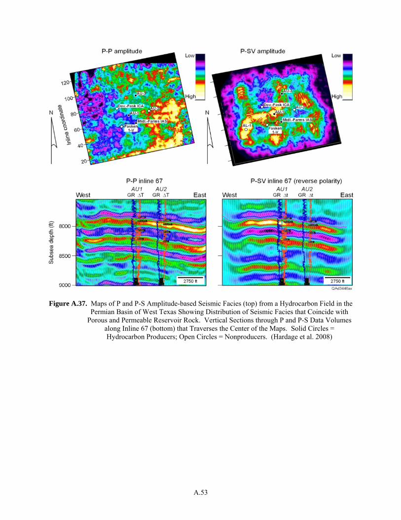
A.53

Figure A.37. Maps of P and P-S Amplitude-based Seismic Facies (top) from a Hydrocarbon Field in the Permian Basin of West Texas Showing Distribution of Seismic Facies that Coincide with

Porous and Permeable Reservoir Rock. Vertical Sections through P and P-S Data Volumes along Inline 67 (bottom) that Traverses the Center of the Maps. Solid Circles = Hydrocarbon Producers; Open Circles = Nonproducers. (Hardage et al. 2008)

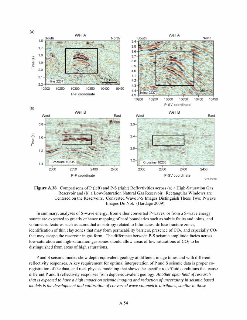
A.54

Figure A.38. Comparisons of P (left) and P-S (right) Reflectivities across (a) a High-Saturation Gas Reservoir and (b) a Low-Saturation Natural Gas Reservoir. Rectangular Windows are

Centered on the Reservoirs. Converted Wave P-S Images Distinguish These Two; P-wave Images Do Not. (Hardage 2009)

In summary, analyses of S-wave energy, from either converted P-waves, or from a S-wave energy source are expected to greatly enhance mapping of hard boundaries such as subtle faults and joints, and volumetric features such as azimuthal anisotropy related to lithofacies, diffuse fracture zones, identification of thin clay zones that may form permeability barriers, presence of CO2, and especially CO2 that may escape the reservoir in gas form. The difference between P-S seismic amplitude facies across low-saturation and high-saturation gas zones should allow areas of low saturations of CO2 to be distinguished from areas of high saturations.

P and S seismic modes show depth-equivalent geology at different image times and with different reflectivity responses. A key requirement for optimal interpretation of P and S seismic data is proper co-registration of the data, and rock physics modeling that shows the specific rock/fluid conditions that cause different P and S reflectivity responses from depth-equivalent geology. Another open field of research that is expected to have a high impact on seismic imaging and reduction of uncertainty in seismic based models is the development and calibration of converted wave volumetric attributes, similar to those

A.55

developed for P-wave data. A newly funded DOE proposal by Hardage (2009) will address the development of converted wave attributes.

A.3.5.3 Seismic Interferometery

The term, interferometery, refers to the study of interference phenomena. Seismic interferometery is a new field of seismic research that takes two parts of the seismic data that are generally filtered out as noise (i.e., codas—the long multiple scattered parts of seismic waveforms, and background noise). These data include a variety of "noise" with periods of either greater or less than one second, and include low frequency background vibrations, train noise, active-source surface waves, earthquake reverberations and more. This technology focuses on unraveling subsurface information from complex waveforms through cross-correlation of pairs of signals and summing (stacking) the data. These simple operations create a virtual seismic source at the geophone receiver (Curtis et al. 2006). This technology not only provides a new means of identifying and subtracting seismic noise due to direct waves and surface waves, but also for time lapse monitoring of CO2 movement in reservoirs such as basalts, where movement of fluids through fractures may have a very small impact on the acoustic impedance.

A.3.5.4 Time Lapse Seismic Surveys

For operational or post operational sequestration fields, carefully repeated 3D surveys provide time-lapse data for MVA (Monitoring, Verification, and Accounting) and dynamic reservoir management. Calibrated seismic amplitude, frequency and other attributes can detect and map CO2 saturation changes and plume movement within or away from the field. Seismic amplitude changes in time-lapse seismic surveys of the Sleipner CO2 sequestration project revealed that CO2 unexpectedly moved up into a sandy facies of the caprock seal (Chadwick et al. 2009).

Time-lapse crosswell seismic and wellbore based VSP can provide greater resolution of local, near wellbore critical velocity data and increased local resolution of features. Microseismic data, when tied to geomechanical data from image logs or other sources, provide calibration for seismic derived field scale fracture and stress patterns. Three D seismic reflection and satellite-based InSAR have been integrated at the basin scale to provide images of millimeter scale surface changes related to subsurface processes (Vasco et al. 2008). In these and other ways, seismic data analysis supports project lifetime activities related to detecting and mapping 3D changes in fluid saturations in heterogeneous reservoirs; pressure or saturation related changes in faults, fractures, and caprock;-and pressure interference from multiple injection or pressure relief wells.

A.3.5.5 Workflows for Developing and Populating Seismic Based Reservoir Models

A workflow for integrating seismic attributes into reservoir characterization is shown in Figure A.39. As a part of best practices workflow, geologic and engineering data are integrated with information from seismic horizon structure mapping and a variety of conventional and new seismic attribute technologies.

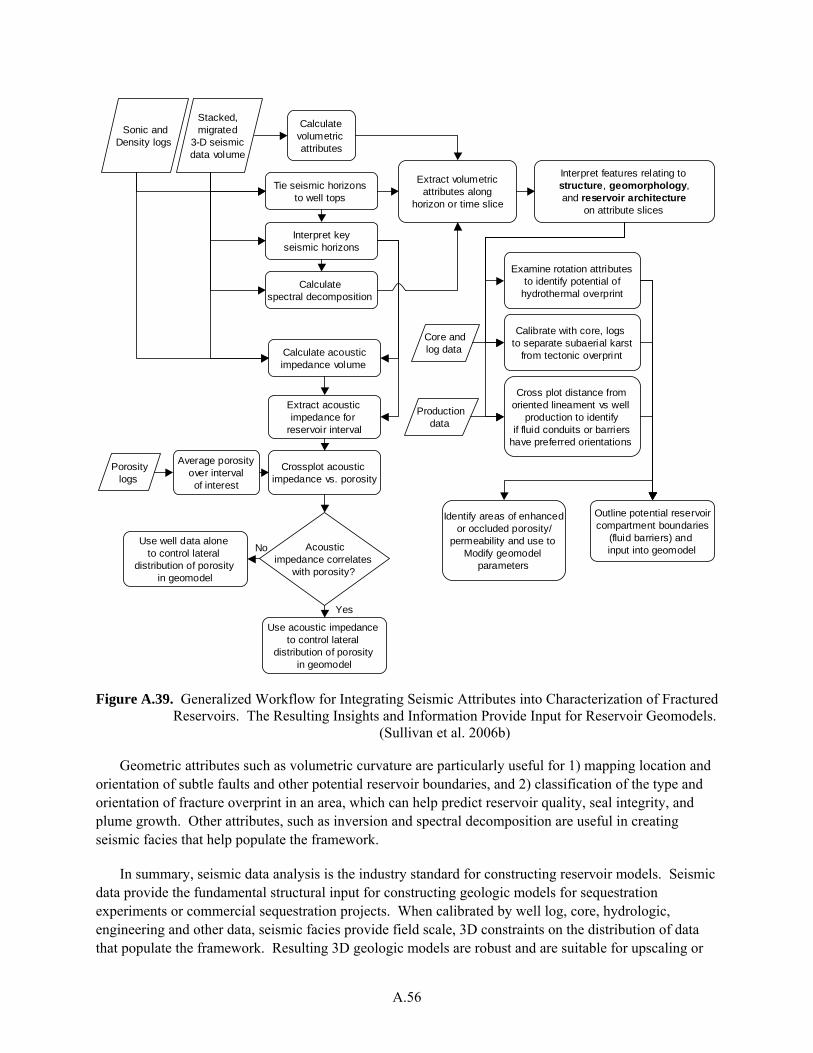
A.56

Tie seismic horizons to well tops

Stacked, migrated

3-D seismic data volume

Sonic andDensity logs

Interpret keyseismic horizons

Calculate acousticimpedance volume

Calculatevolumetric attributes

Extract volumetricattributes along

horizon or time slice

Porositylogs

Extract acoustic impedance for

reservoir interval

Interpret features relating to structure, geomorphology,and reservoir architecture

on attribute slices

Acousticimpedance correlates

with porosity?

Crossplot acoustic impedance vs. porosity

Use acoustic impedance to control lateral

distribution of porosity in geomodel

Average porosityover intervalof interest

Examine rotation attributesto identify potential of

hydrothermal overprint

Calibrate with core, logs to separate subaerial karst

from tectonic overprint

Cross plot distance fromoriented lineament vs well

production to identifyif fluid conduits or barriers

have preferred orientations

Outline potential reservoircompartment boundaries

(fluid barriers) and input into geomodel

Identify areas of enhancedor occluded porosity/

permeability and use to Modify geomodel

parameters

Yes

Use well data alone to control lateral

distribution of porosity in geomodel

No

Calculate spectral decomposition

Core andlog data

Productiondata

Figure A.39. Generalized Workflow for Integrating Seismic Attributes into Characterization of Fractured Reservoirs. The Resulting Insights and Information Provide Input for Reservoir Geomodels.

(Sullivan et al. 2006b)

Geometric attributes such as volumetric curvature are particularly useful for 1) mapping location and orientation of subtle faults and other potential reservoir boundaries, and 2) classification of the type and orientation of fracture overprint in an area, which can help predict reservoir quality, seal integrity, and plume growth. Other attributes, such as inversion and spectral decomposition are useful in creating seismic facies that help populate the framework.

In summary, seismic data analysis is the industry standard for constructing reservoir models. Seismic data provide the fundamental structural input for constructing geologic models for sequestration experiments or commercial sequestration projects. When calibrated by well log, core, hydrologic, engineering and other data, seismic facies provide field scale, 3D constraints on the distribution of data that populate the framework. Resulting 3D geologic models are robust and are suitable for upscaling or

A.57

subdividing and upscaling into 3D blocks for simulation. For field operations, seismic based models will provide the fundamental basis for siting individual injection and monitoring wells, in addition to development of MVA programs and lea.k.a.ge mitigation plans. There is an ever-growing variety of seismic attributes and techniques for enhancing recognition and interpretation of subsurface features that are relevant or critical to sequestration.

For operational or post operational sequestration fields, carefully repeated 3D surveys provide time-lapse data for MVA and dynamic reservoir management. Calibrated seismic amplitude, frequency and other attributes can detect and map CO2 saturation changes and plume movement within or away from the field. Crosswell seismic and wellbore based VSP provide critical velocity data and increased local resolution of features. Microseismic data, when tied to geomechanical data from image logs or other sources, provide calibration for seismic derived field scale fracture and stress patterns. Three-dimensional seismic reflection and satellite based InSAR have been integrated at the basin scale to provide images of millimeter scale surface changes related to subsurface processes (Arts et al. 2004, Vasco et al. 2008). In these and other ways, seismic data analysis supports project lifetime activities related to detecting and mapping 3D changes in fluid saturations in heterogeneous reservoirs; pressure or saturation related changes in faults, fractures, and caprock;-and pressure interference from multiple injection or pressure relief wells. The rock physics basis for calibration of CO2 saturations to 3D seismic attribute signature is still in its infancy and represents a major opportunity for research and innovation.

A.4 Geomechanical Data Analysis

There are several types of geomechanical considerations that are critical, but often underplayed in carbon sequestration. These include analysis of the initial earth stresses at the wellbore, and along faults and fractures of different types and orientations near and at a distance to the wellbore. Hydrodynamic pressures generated by injection or withdrawal of fluids may affect the direction of CO2 flow or migration and the stability of faults and fractures in the reservoir and caprock. There has been little study on the effect of pressure interference from multiple injectors, or effects of phase changes that may occur during natural leakage.

The permeability of many aquifers and hydrocarbon reservoirs are dominated by fracture flow. In other situations, fractures may be short, and may be restricted to certain beds or lithologies. If a ductile shale is sandwiched between two brittle limestone layers, folding or bending all the layers may produce fractures in the limestone, but not in the shale.

Barton et al. (1995) and Zoback (1996) have shown through borehole measurements that there is preferential flow along joints aligned in the direction of maximum activation with respect to the principal stress direction. Specifically, as the shear stress induced on faults and fractures approaches the friction limit, such fractures are observed to become conduits for fluid flow.

Geomechanical data are incorporated in reservoir models through 3D grids of fracture planes, or added as maps of particular horizons. Fault population statistics can be developed from existing coverage of regional stress, faults and other data during the site selection phase, and improved as site characterization progresses. The field of fault population statistics is relatively well developed and is applied in the oil and gas industry, as it relates to reservoir performance, compartmentalization, and seal integrity (Needham et al. 1996). In geologic carbon sequestration, fault population statistics are one

A.58

approach to determining the probability of a plume encountering a fault, both prior to the availability of more deterministic information, and with regard to features below the resolution limit of the characterization methods applied (Jordan et al. 2008).

Seismic methods are a standard technology to detect joints and faults in reservoirs and seals. Two of the primary effects on the seismic wavefield are anisotropy in the propagation velocity (Helbig and Thomsen 2005) and attenuation of the seismic energy. Although seismic resolution of joints and faults is limited, borehole, crosswell and microseismic data provide calibration for identification of field scale lineaments observed in 3-D seismic. Curvature and other modern 3D seismic attributes can detect faults and joint sets, perhaps to 0.1 of a seismic wavelength (Chopra and Marfurt 2007), but we are still indirectly observing the effects of faults and joints in the seismic response. Except for new frequency attributes associated with frequency and seismic attenuation (Goloshubin and Silin 2006), we are not observing a seismic signature directly related to effects of permeability. The recent advances in wellbore estimation of permeability with acoustic Stoneley waves represents a breakthrough for calibration of seismic frequency and attenuation attributes.

A.4.1 Types of Data

Fracture is a general term for any mechanical discontinuity that represents a zone of brittle mechanical failure3. Joints and faults are types of fractures. A fault is a joint along which movement has occurred. The relation of fracture formation to earth stresses is illustrated in Figure A.40; stylolites (blue zig-zag features) are formed by compression, dissolution of rock (usually carbonate) and accumulation of insoluable residues. Stylolites form perpendicular to the major stress, and are generally closed in this orientation, but can open if the stress orientation changes. Regional and local earth stress data are essential to determine site stability and to determine which faults and fractures lie close to critical angles for failure and to quantify the increase in reservoir pressures that would cause faults to slip and existing fractures to open. Regional stress maps (Zoback and Zoback 1980) give general information on whether an area is in a compressional, tensional, strike slip or combination setting. It is important to note that stress regimes change in four dimensions. Stress orientations observed in surface geology may have no relation to stress regime in a deep sequestration zone.

3 Lacazette http://www.naturalfractures.com

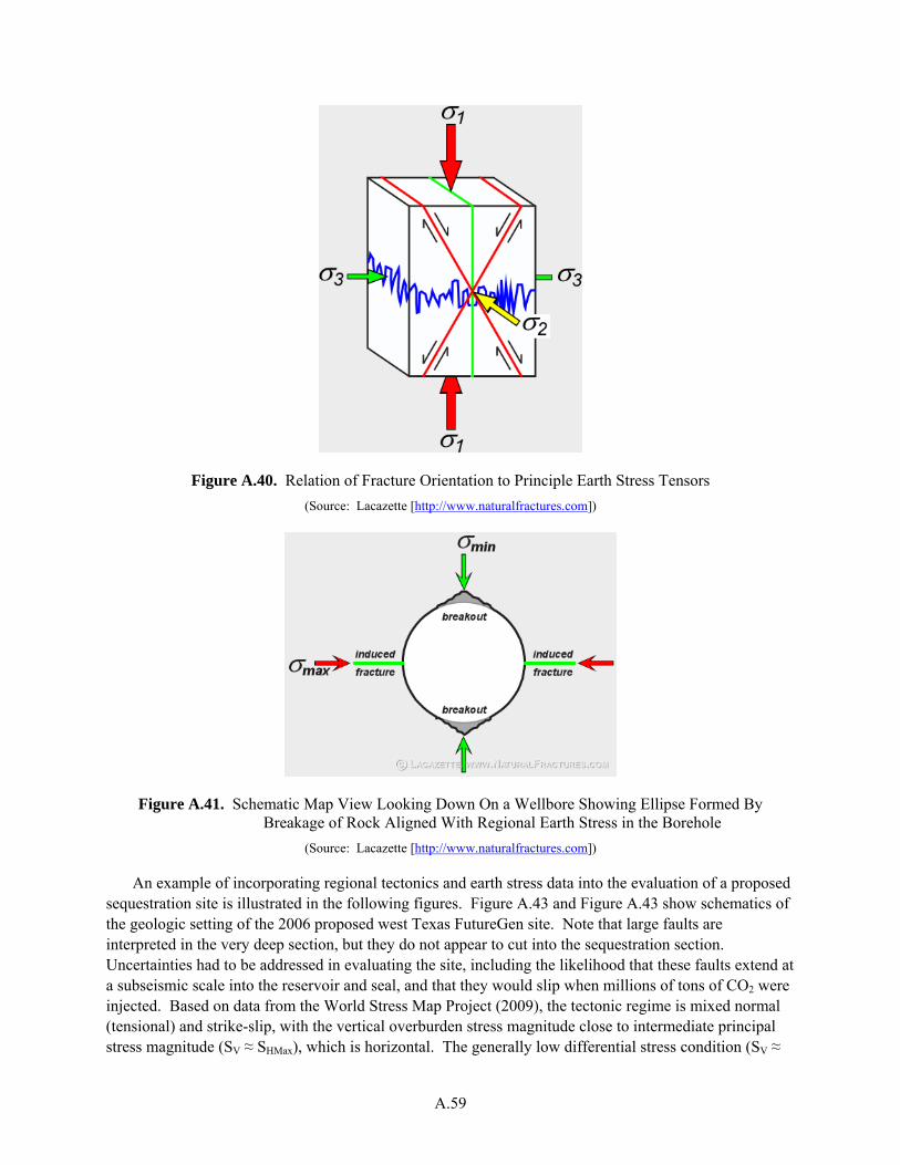
A.59

Figure A.40. Relation of Fracture Orientation to Principle Earth Stress Tensors (Source: Lacazette [http://www.naturalfractures.com])

Figure A.41. Schematic Map View Looking Down On a Wellbore Showing Ellipse Formed By Breakage of Rock Aligned With Regional Earth Stress in the Borehole

(Source: Lacazette [http://www.naturalfractures.com])

An example of incorporating regional tectonics and earth stress data into the evaluation of a proposed sequestration site is illustrated in the following figures. Figure A.43 and Figure A.43 show schematics of the geologic setting of the 2006 proposed west Texas FutureGen site. Note that large faults are interpreted in the very deep section, but they do not appear to cut into the sequestration section. Uncertainties had to be addressed in evaluating the site, including the likelihood that these faults extend at a subseismic scale into the reservoir and seal, and that they would slip when millions of tons of CO2 were injected. Based on data from the World Stress Map Project (2009), the tectonic regime is mixed normal (tensional) and strike-slip, with the vertical overburden stress magnitude close to intermediate principal stress magnitude (SV ≈ SHMax), which is horizontal. The generally low differential stress condition (SV ≈

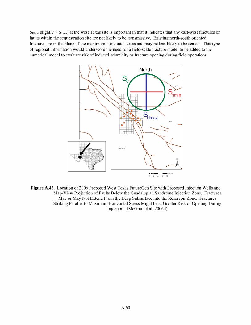
A.60

SHMax slightly > Shmin) at the west Texas site is important in that it indicates that any east-west fractures or faults within the sequestration site are not likely to be transmissive. Existing north-south oriented fractures are in the plane of the maximum horizontal stress and may be less likely to be sealed. This type of regional information would underscore the need for a field-scale fracture model to be added to the numerical model to evaluate risk of induced seismicity or fracture opening during field operations.

North

Shmin

SHmax

SV

Figure A.42. Location of 2006 Proposed West Texas FutureGen Site with Proposed Injection Wells and Map-View Projection of Faults Below the Guadalupian Sandstone Injection Zone. Fractures

May or May Not Extend From the Deep Subsurface into the Reservoir Zone. Fractures Striking Parallel to Maximum Horizontal Stress Might be at Greater Risk of Opening During

Injection. (McGrail et al. 2006d)

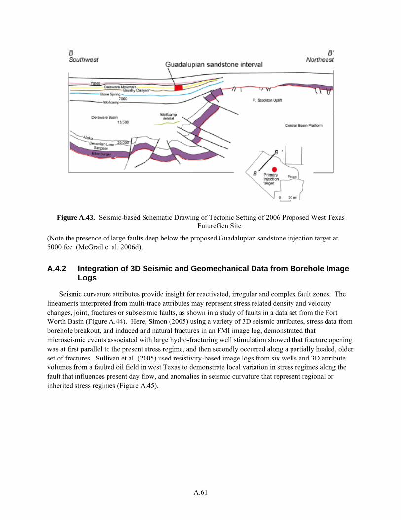
A.61

Figure A.43. Seismic-based Schematic Drawing of Tectonic Setting of 2006 Proposed West Texas FutureGen Site

(Note the presence of large faults deep below the proposed Guadalupian sandstone injection target at 5000 feet (McGrail et al. 2006d).

A.4.2 Integration of 3D Seismic and Geomechanical Data from Borehole Image Logs

Seismic curvature attributes provide insight for reactivated, irregular and complex fault zones. The lineaments interpreted from multi-trace attributes may represent stress related density and velocity changes, joint, fractures or subseismic faults, as shown in a study of faults in a data set from the Fort Worth Basin (Figure A.44). Here, Simon (2005) using a variety of 3D seismic attributes, stress data from borehole breakout, and induced and natural fractures in an FMI image log, demonstrated that microseismic events associated with large hydro-fracturing well stimulation showed that fracture opening was at first parallel to the present stress regime, and then secondly occurred along a partially healed, older set of fractures. Sullivan et al. (2005) used resistivity-based image logs from six wells and 3D attribute volumes from a faulted oil field in west Texas to demonstrate local variation in stress regimes along the fault that influences present day flow, and anomalies in seismic curvature that represent regional or inherited stress regimes (Figure A.45).

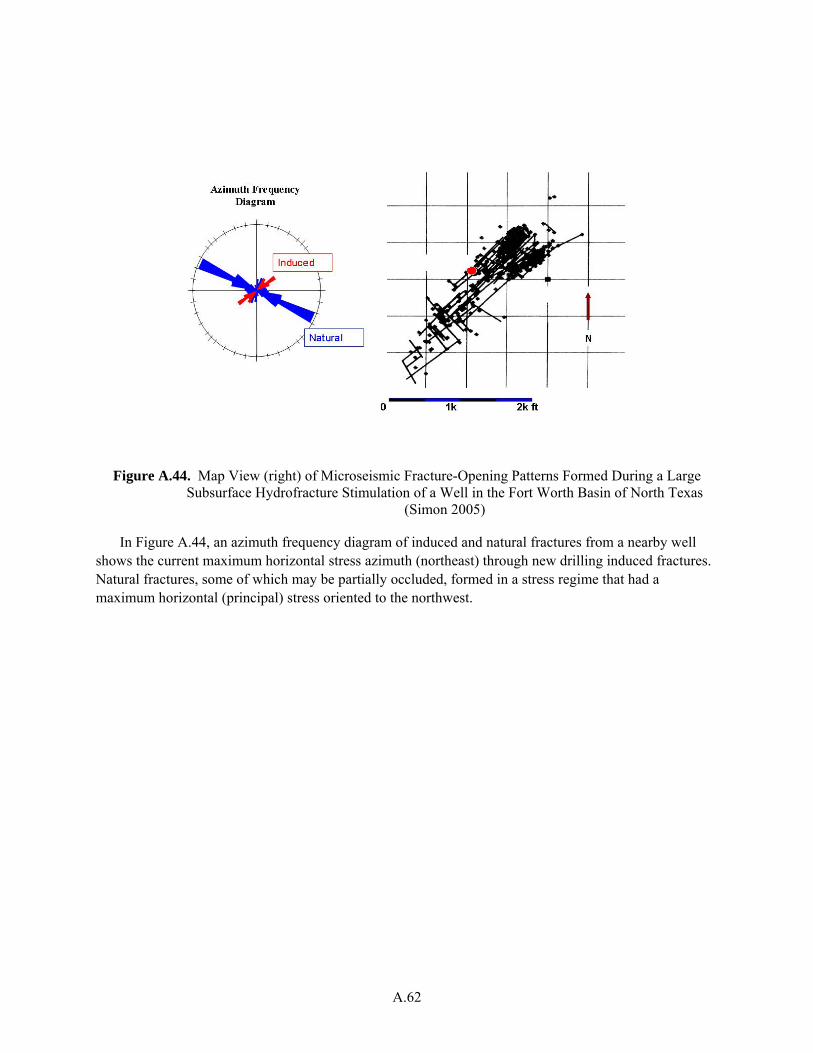
A.62

Figure A.44. Map View (right) of Microseismic Fracture-Opening Patterns Formed During a Large Subsurface Hydrofracture Stimulation of a Well in the Fort Worth Basin of North Texas

(Simon 2005)

In Figure A.44, an azimuth frequency diagram of induced and natural fractures from a nearby well shows the current maximum horizontal stress azimuth (northeast) through new drilling induced fractures. Natural fractures, some of which may be partially occluded, formed in a stress regime that had a maximum horizontal (principal) stress oriented to the northwest.

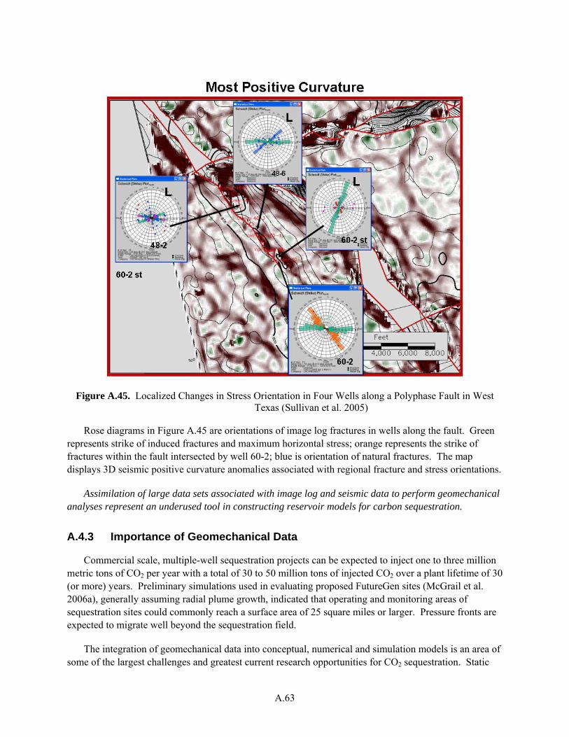
A.63

Figure A.45. Localized Changes in Stress Orientation in Four Wells along a Polyphase Fault in West Texas (Sullivan et al. 2005)

Rose diagrams in Figure A.45 are orientations of image log fractures in wells along the fault. Green represents strike of induced fractures and maximum horizontal stress; orange represents the strike of fractures within the fault intersected by well 60-2; blue is orientation of natural fractures. The map displays 3D seismic positive curvature anomalies associated with regional fracture and stress orientations.

Assimilation of large data sets associated with image log and seismic data to perform geomechanical analyses represent an underused tool in constructing reservoir models for carbon sequestration.

A.4.3 Importance of Geomechanical Data

Commercial scale, multiple-well sequestration projects can be expected to inject one to three million metric tons of CO2 per year with a total of 30 to 50 million tons of injected CO2 over a plant lifetime of 30 (or more) years. Preliminary simulations used in evaluating proposed FutureGen sites (McGrail et al. 2006a), generally assuming radial plume growth, indicated that operating and monitoring areas of sequestration sites could commonly reach a surface area of 25 square miles or larger. Pressure fronts are expected to migrate well beyond the sequestration field.

The integration of geomechanical data into conceptual, numerical and simulation models is an area of some of the largest challenges and greatest current research opportunities for CO2 sequestration. Static

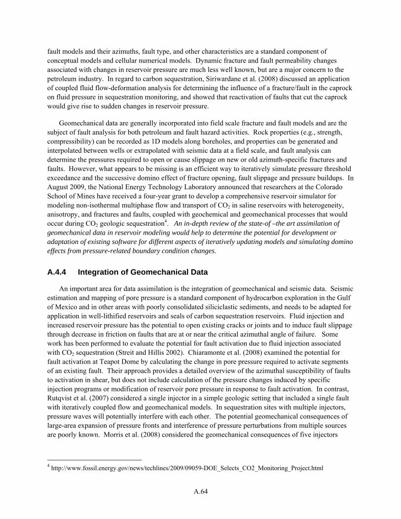
A.64

fault models and their azimuths, fault type, and other characteristics are a standard component of conceptual models and cellular numerical models. Dynamic fracture and fault permeability changes associated with changes in reservoir pressure are much less well known, but are a major concern to the petroleum industry. In regard to carbon sequestration, Siriwardane et al. (2008) discussed an application of coupled fluid flow-deformation analysis for determining the influence of a fracture/fault in the caprock on fluid pressure in sequestration monitoring, and showed that reactivation of faults that cut the caprock would give rise to sudden changes in reservoir pressure.

Geomechanical data are generally incorporated into field scale fracture and fault models and are the subject of fault analysis for both petroleum and fault hazard activities. Rock properties (e.g., strength, compressibility) can be recorded as 1D models along boreholes, and properties can be generated and interpolated between wells or extrapolated with seismic data at a field scale, and fault analysis can determine the pressures required to open or cause slippage on new or old azimuth-specific fractures and faults. However, what appears to be missing is an efficient way to iteratively simulate pressure threshold exceedance and the successive domino effect of fracture opening, fault slippage and pressure buildups. In August 2009, the National Energy Technology Laboratory announced that researchers at the Colorado School of Mines have received a four-year grant to develop a comprehensive reservoir simulator for modeling non-isothermal multiphase flow and transport of CO2 in saline reservoirs with heterogeneity, anisotropy, and fractures and faults, coupled with geochemical and geomechanical processes that would occur during CO2 geologic sequestration4. An in-depth review of the state-of –the art assimilation of geomechanical data in reservoir modeling would help to determine the potential for development or adaptation of existing software for different aspects of iteratively updating models and simulating domino effects from pressure-related boundary condition changes.

A.4.4 Integration of Geomechanical Data

An important area for data assimilation is the integration of geomechanical and seismic data. Seismic estimation and mapping of pore pressure is a standard component of hydrocarbon exploration in the Gulf of Mexico and in other areas with poorly consolidated siliciclastic sediments, and needs to be adapted for application in well-lithified reservoirs and seals of carbon sequestration reservoirs. Fluid injection and increased reservoir pressure has the potential to open existing cracks or joints and to induce fault slippage through decrease in friction on faults that are at or near the critical azimuthal angle of failure. Some work has been performed to evaluate the potential for fault activation due to fluid injection associated with CO2 sequestration (Streit and Hillis 2002). Chiaramonte et al. (2008) examined the potential for fault activation at Teapot Dome by calculating the change in pore pressure required to activate segments of an existing fault. Their approach provides a detailed overview of the azimuthal susceptibility of faults to activation in shear, but does not include calculation of the pressure changes induced by specific injection programs or modification of reservoir pore pressure in response to fault activation. In contrast, Rutqvist et al. (2007) considered a single injector in a simple geologic setting that included a single fault with iteratively coupled flow and geomechanical models. In sequestration sites with multiple injectors, pressure waves will potentially interfere with each other. The potential geomechanical consequences of large-area expansion of pressure fronts and interference of pressure perturbations from multiple sources are poorly known. Morris et al. (2008) considered the geomechanical consequences of five injectors

4 http://www.fossil.energy.gov/news/techlines/2009/09059-DOE_Selects_CO2_Monitoring_Project.html

A.65

operated in the presence of several faults, but assumed a simplified geometry to aid in coupling between the hydrologic and geomechanical codes.

A number of groups are interested in developing a multi-sensor geophysical toolbox for monitoring and quantifying subsurface processes and events associated with initiating, operating and closing sequestration experiments and commercial operations. The most commonly envisioned toolboxes build on current oil field, remediation, gas storage, and other activities that involve the remote monitoring, collection, and telemetry of real time data to a central server that processes, interprets and generates customized visualizations for multiple types of users. A typical geophysical toolbox for CO2 MVA activities might consist of a permanent, autonomous and automated sensor network with passive micro-seismic sensors, electrical geophysical sensors, tiltmeters, and gravity sensors, along with and middleware and processing software. Many of these geophysical methods have demonstrated value for long-term monitoring (Daily et al. 2008). Co-located remote monitoring and telemetry technologies such as the oilfield standard SCADA (Supervisory Control and Data Acquisition) technologies would relay pressure, temperature and various geochemical data to a central location for analysis and response, and shut down the injection if pressures or other data moved beyond certain limits. The development, modification, and testing of new and existing techniques to assimilate these types and volumes of data with geomechanical data represent an opportunity to create new attributes for quantifying and mapping temporal and spatial changes of CO2 saturations and phases, as well as mapping and predicting fracture and fault behavior, growth and interference of pressure fronts, and other dynamic aspects of reservoir sequestration.

A.5 Solid-Earth Modeling

Solid earth modeling is the process of constructing a three-dimensional model of a portion of the earth that will reflect the distribution of whatever geological units and/or properties are of interest. For the specific purpose of designing and evaluating a carbon dioxide sequestration project, the solid earth model will, at a minimum, incorporate the geometry of the target reservoir and whatever geologic unit or units that form the cap rock. It may also include other intermediate or overlying geologic units. The model may incorporate faults that offset unit contacts and act as either barriers or conduits to fluid flow. Physical, chemical, lithological and mechanical properties within one or more geologic unit are also often of interest and can be assigned as a constant or a distribution within the solid earth model.

The advantages of a solid earth model are the ability to link the input data to the model building process, create visualizations of different parts of the model, and export information to numerical models used to simulate flow or mechanical processes. Output from these external modeling processes can then be merged with the solid earth model for combined visualization of simulation results and geologic structures. Software for solid earth modeling also often facilitates keeping track of input data and changes to the model.

Building the solid earth model generally consists of the following steps. However, some of these may not apply depending on the complexity of the project and the types of available data:

• determine the model domain:

– scale

– horizontal units and coordinate system

A.66

– vertical units

• obtain, convert, import and edit input data:

– borehole lithologic contact depths

– fault depths at boreholes

– seismic data

– geophysical logs

– property measurements

• perform seismic visualization and interpretation

• correlate seismic data structures to borehole lithologic contacts

• generate faults:

– define fault characteristics (dying or extensive)

– model fault planes

– determine offsets

• perform seismic depth conversions

• generate unit contact horizons (surfaces with fault breaks)

• model facies or property distributions throughout specific geologic units

• build solid earth model

• calculate volumes

• generate visualizations of the results

• evaluate results and compare to input data

• revise model based on new or revised input data.

Several different solid earth modeling software packages exist. Two that are currently in use at PNNL are Earthvision™ from Dynamic Graphics, Inc. and Petrel™ from Schlumberger. Further discussion on these software packages is provided in the appendix. Figure A.46 shows a cutaway view of a portion of the Teapot Dome Field in Wyoming generated using EarthVision™.

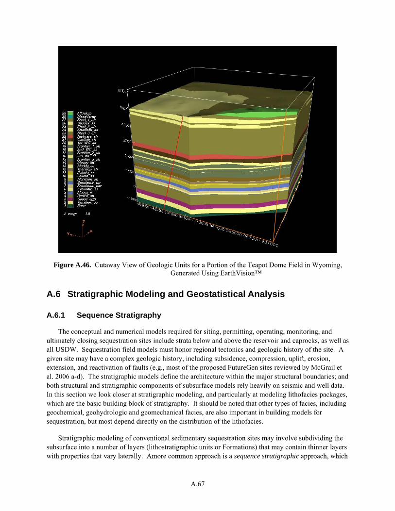
A.67

Figure A.46. Cutaway View of Geologic Units for a Portion of the Teapot Dome Field in Wyoming, Generated Using EarthVision™

A.6 Stratigraphic Modeling and Geostatistical Analysis

A.6.1 Sequence Stratigraphy

The conceptual and numerical models required for siting, permitting, operating, monitoring, and ultimately closing sequestration sites include strata below and above the reservoir and caprocks, as well as all USDW. Sequestration field models must honor regional tectonics and geologic history of the site. A given site may have a complex geologic history, including subsidence, compression, uplift, erosion, extension, and reactivation of faults (e.g., most of the proposed FutureGen sites reviewed by McGrail et al. 2006 a-d). The stratigraphic models define the architecture within the major structural boundaries; and both structural and stratigraphic components of subsurface models rely heavily on seismic and well data. In this section we look closer at stratigraphic modeling, and particularly at modeling lithofacies packages, which are the basic building block of stratigraphy. It should be noted that other types of facies, including geochemical, geohydrologic and geomechanical facies, are also important in building models for sequestration, but most depend directly on the distribution of the lithofacies.

Stratigraphic modeling of conventional sedimentary sequestration sites may involve subdividing the subsurface into a number of layers (lithostratigraphic units or Formations) that may contain thinner layers with properties that vary laterally. Amore common approach is a sequence stratigraphic approach, which

A.68

involves identifying small-scale (3-30 ft thick) rock packages of genetically related strata within large-scale (100-300 ft thick) time-stratigraphic packages, whose boundaries are surfaces of erosion, or non-deposition. Basinward, these major time-stratigraphic surfaces may laterally grade into strata that record continuous deposition (Posamentier et al. 1988, van Wagoner et al. 1990). Sequence stratigraphy is differentiated from lithostratigraphy in that sequence stratigraphy is used to correlate time-related packages of depositional facies that are separated from other large packages by boundaries that reflect eustatic (global) sea level changes. This is the basis of most hydrocarbon exploration in large basins such as the Gulf of Mexico, where the age of major sea level drops associated with erosional sequence boundaries are dated by fossils and other data.

More time is represented by a major unconformity at the edge of a basin, or over areas of repeated tectonic warping and uplift, such as the interior of continents. For example, The Ozark dome, the site of a Great Plains Sequestration Partnership project, is characterized by thin Paleozoic sandstones and carbonates, abundant unconformities representing long time spans of erosion and/or non-deposition, and a very shallow depth to Precambrian granitic basement. In areas such as this, the entire porous sedimentary column may be only 500-600m thick, too thin for maintaining CO2 in a supercritical phase. In contrast, thick packages of sediment may accumulate in continental areas that have experienced considerable subsidence or down warping, such as the Michigan Basin, the Illinois Basin, the Appalachian Basin or the Permian Basin. Even in those areas of thick accumulation, sedimentary rock s can be subdivided into packages or sequences that reflect changes in sediment accommodation space (water depth), sediment supply, climate, tectonics, eustatic sea level changes, and landward and seaward changes in geographic location of the shoreline. Changes in sediment and depositional environments affect reservoir and seal porosity, permeability and heterogeneity.

The depositional setting from onshore to offshore is called a facies tract; facies tracts are separated by small scale unconformities into lowstand, highstand, and other packages related to the position of sea level and the depositional environment. In essence, reservoir scale stratigraphic sequences are each composed of a succession of genetically linked strata that reflect deposition in natural, depositional systems (e.g., low stand, high stand systems tracts) that are interpreted to have been deposited between eustatic sea-level fall inflection points (Posamentier et al. 1988).

The power of a sequence-stratigraphic-based conceptual model is the ability to predict stratigraphic location, thickness, and azimuthal trend of reservoir bodies, development and continuity of seals, rock properties, fracture systems (Zahm et al. 2009), karst features (e.g. collapsed caverns) in carbonates, and much more. For example, karst features in the Knox carbonates, controlled by unconformities associated with sea level fall, are a major potential drilling hazard at the Illinois carbon sequestration sites.

Figure A.47 shows two successive steps (A and B) in the deposition of sand (dotted pattern), shale (dashed pattern) and carbonates (brick pattern) in a shallow marine environment as sea level advances landward (to the left). Maximum transgression is the Maximum Flooding zone or surface, which is one of the most common sources of regional seals for CO2 sequestration. A slowing of the relative rise in sea level allows sediments to prograde seaward, as indicated in Figure A.47C. If sea level rise and sediment supply were to balance perfectly, a thick sand wedge would accumulate as an agradational package. This is one way that very attractive regional sequestration targets may form, such as the 300 ft thick St Peter sandstones in Michigan, or certain Cenozoic wave-dominated delta sandstones in the subsurface of the U.S. Gulf Coast.

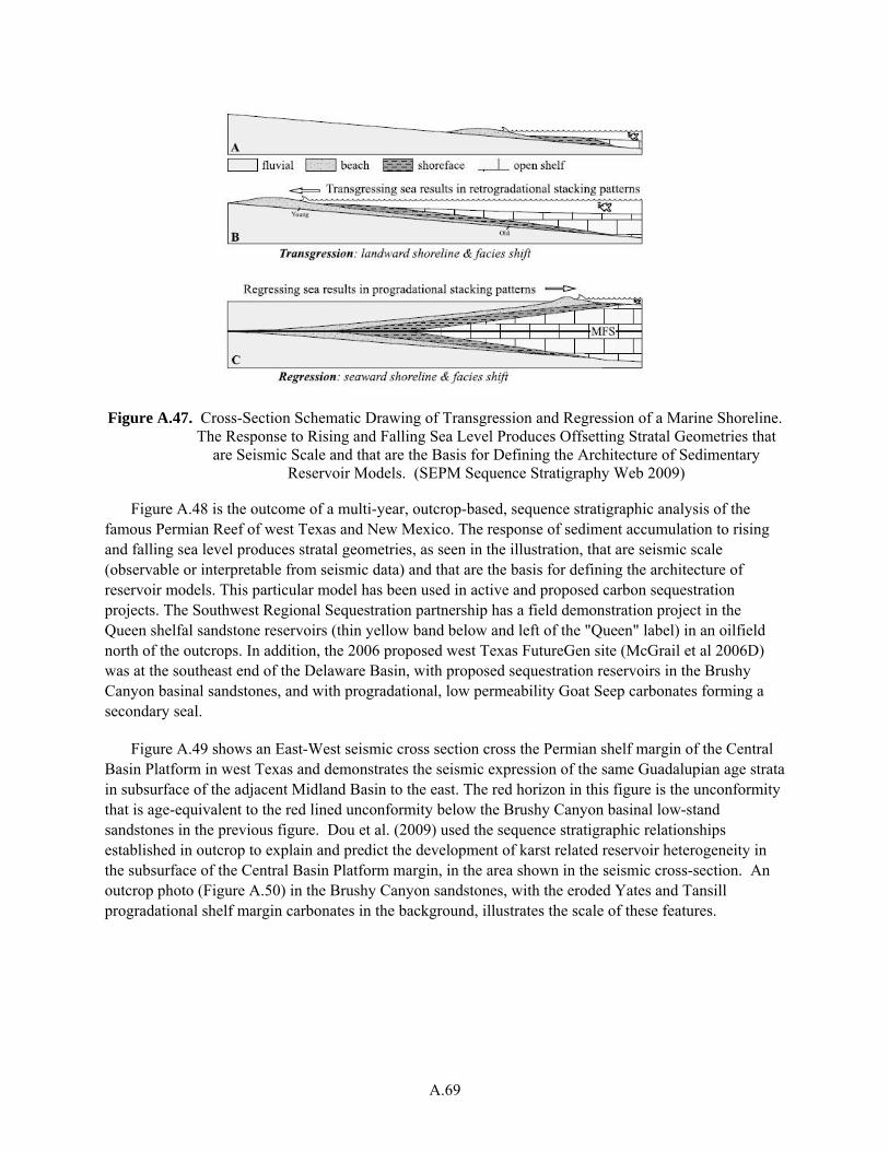
A.69

Figure A.47. Cross-Section Schematic Drawing of Transgression and Regression of a Marine Shoreline. The Response to Rising and Falling Sea Level Produces Offsetting Stratal Geometries that

are Seismic Scale and that are the Basis for Defining the Architecture of Sedimentary Reservoir Models. (SEPM Sequence Stratigraphy Web 2009)

Figure A.48 is the outcome of a multi-year, outcrop-based, sequence stratigraphic analysis of the famous Permian Reef of west Texas and New Mexico. The response of sediment accumulation to rising and falling sea level produces stratal geometries, as seen in the illustration, that are seismic scale (observable or interpretable from seismic data) and that are the basis for defining the architecture of reservoir models. This particular model has been used in active and proposed carbon sequestration projects. The Southwest Regional Sequestration partnership has a field demonstration project in the Queen shelfal sandstone reservoirs (thin yellow band below and left of the "Queen" label) in an oilfield north of the outcrops. In addition, the 2006 proposed west Texas FutureGen site (McGrail et al 2006D) was at the southeast end of the Delaware Basin, with proposed sequestration reservoirs in the Brushy Canyon basinal sandstones, and with progradational, low permeability Goat Seep carbonates forming a secondary seal.

Figure A.49 shows an East-West seismic cross section cross the Permian shelf margin of the Central Basin Platform in west Texas and demonstrates the seismic expression of the same Guadalupian age strata in subsurface of the adjacent Midland Basin to the east. The red horizon in this figure is the unconformity that is age-equivalent to the red lined unconformity below the Brushy Canyon basinal low-stand sandstones in the previous figure. Dou et al. (2009) used the sequence stratigraphic relationships established in outcrop to explain and predict the development of karst related reservoir heterogeneity in the subsurface of the Central Basin Platform margin, in the area shown in the seismic cross-section. An outcrop photo (Figure A.50) in the Brushy Canyon sandstones, with the eroded Yates and Tansill progradational shelf margin carbonates in the background, illustrates the scale of these features.

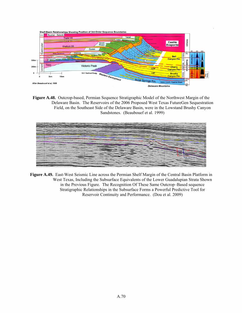
A.70

Figure A.48. Outcrop-based, Permian Sequence Stratigraphic Model of the Northwest Margin of the Delaware Basin. The Reservoirs of the 2006 Proposed West Texas FutureGen Sequestration

Field, on the Southeast Side of the Delaware Basin, were in the Lowstand Brushy Canyon Sandstones. (Beaubouef et al. 1999)

Figure A.49. East-West Seismic Line across the Permian Shelf Margin of the Central Basin Platform in West Texas, Including the Subsurface Equivalents of the Lower Guadalupian Strata Shown

in the Previous Figure. The Recognition Of These Same Outcrop–Based sequence Stratigraphic Relationships in the Subsurface Forms a Powerful Predictive Tool for

Reservoir Continuity and Performance. (Dou et al. 2009)

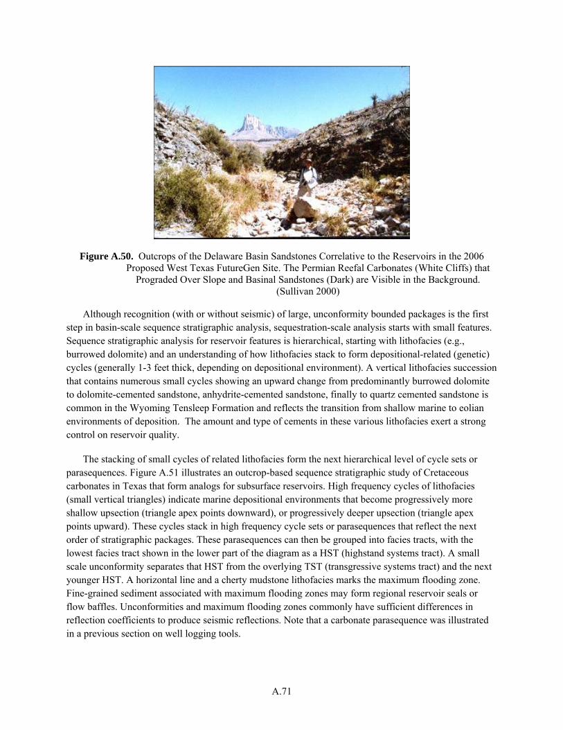
A.71

Figure A.50. Outcrops of the Delaware Basin Sandstones Correlative to the Reservoirs in the 2006 Proposed West Texas FutureGen Site. The Permian Reefal Carbonates (White Cliffs) that

Prograded Over Slope and Basinal Sandstones (Dark) are Visible in the Background. (Sullivan 2000)

Although recognition (with or without seismic) of large, unconformity bounded packages is the first step in basin-scale sequence stratigraphic analysis, sequestration-scale analysis starts with small features. Sequence stratigraphic analysis for reservoir features is hierarchical, starting with lithofacies (e.g., burrowed dolomite) and an understanding of how lithofacies stack to form depositional-related (genetic) cycles (generally 1-3 feet thick, depending on depositional environment). A vertical lithofacies succession that contains numerous small cycles showing an upward change from predominantly burrowed dolomite to dolomite-cemented sandstone, anhydrite-cemented sandstone, finally to quartz cemented sandstone is common in the Wyoming Tensleep Formation and reflects the transition from shallow marine to eolian environments of deposition. The amount and type of cements in these various lithofacies exert a strong control on reservoir quality.

The stacking of small cycles of related lithofacies form the next hierarchical level of cycle sets or parasequences. Figure A.51 illustrates an outcrop-based sequence stratigraphic study of Cretaceous carbonates in Texas that form analogs for subsurface reservoirs. High frequency cycles of lithofacies (small vertical triangles) indicate marine depositional environments that become progressively more shallow upsection (triangle apex points downward), or progressively deeper upsection (triangle apex points upward). These cycles stack in high frequency cycle sets or parasequences that reflect the next order of stratigraphic packages. These parasequences can then be grouped into facies tracts, with the lowest facies tract shown in the lower part of the diagram as a HST (highstand systems tract). A small scale unconformity separates that HST from the overlying TST (transgressive systems tract) and the next younger HST. A horizontal line and a cherty mudstone lithofacies marks the maximum flooding zone. Fine-grained sediment associated with maximum flooding zones may form regional reservoir seals or flow baffles. Unconformities and maximum flooding zones commonly have sufficient differences in reflection coefficients to produce seismic reflections. Note that a carbonate parasequence was illustrated in a previous section on well logging tools.

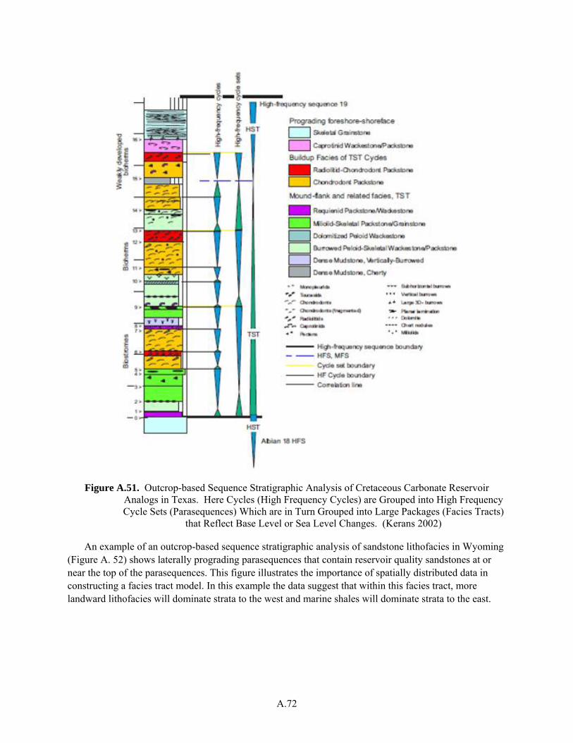
A.72

Figure A.51. Outcrop-based Sequence Stratigraphic Analysis of Cretaceous Carbonate Reservoir Analogs in Texas. Here Cycles (High Frequency Cycles) are Grouped into High Frequency Cycle Sets (Parasequences) Which are in Turn Grouped into Large Packages (Facies Tracts)

that Reflect Base Level or Sea Level Changes. (Kerans 2002)

An example of an outcrop-based sequence stratigraphic analysis of sandstone lithofacies in Wyoming (Figure A. 52) shows laterally prograding parasequences that contain reservoir quality sandstones at or near the top of the parasequences. This figure illustrates the importance of spatially distributed data in constructing a facies tract model. In this example the data suggest that within this facies tract, more landward lithofacies will dominate strata to the west and marine shales will dominate strata to the east.

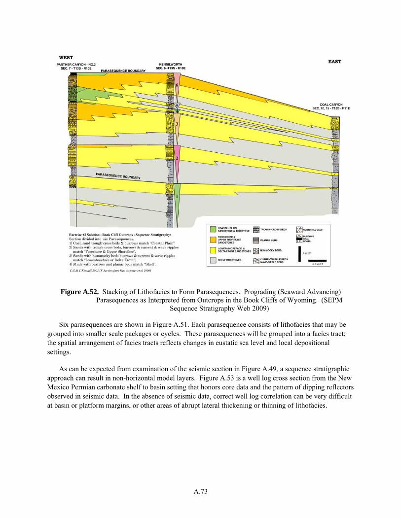
A.73

Figure A.52. Stacking of Lithofacies to Form Parasequences. Prograding (Seaward Advancing) Parasequences as Interpreted from Outcrops in the Book Cliffs of Wyoming. (SEPM

Sequence Stratigraphy Web 2009)

Six parasequences are shown in Figure A.51. Each parasequence consists of lithofacies that may be grouped into smaller scale packages or cycles. These parasequences will be grouped into a facies tract; the spatial arrangement of facies tracts reflects changes in eustatic sea level and local depositional settings.

As can be expected from examination of the seismic section in Figure A.49, a sequence stratigraphic approach can result in non-horizontal model layers. Figure A.53 is a well log cross section from the New Mexico Permian carbonate shelf to basin setting that honors core data and the pattern of dipping reflectors observed in seismic data. In the absence of seismic data, correct well log correlation can be very difficult at basin or platform margins, or other areas of abrupt lateral thickening or thinning of lithofacies.

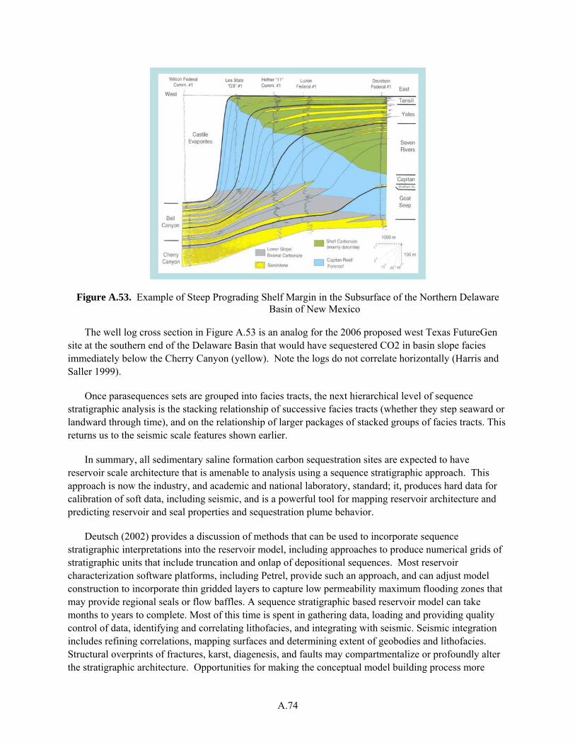
A.74

Figure A.53. Example of Steep Prograding Shelf Margin in the Subsurface of the Northern Delaware Basin of New Mexico

The well log cross section in Figure A.53 is an analog for the 2006 proposed west Texas FutureGen site at the southern end of the Delaware Basin that would have sequestered CO2 in basin slope facies immediately below the Cherry Canyon (yellow). Note the logs do not correlate horizontally (Harris and Saller 1999).

Once parasequences sets are grouped into facies tracts, the next hierarchical level of sequence stratigraphic analysis is the stacking relationship of successive facies tracts (whether they step seaward or landward through time), and on the relationship of larger packages of stacked groups of facies tracts. This returns us to the seismic scale features shown earlier.

In summary, all sedimentary saline formation carbon sequestration sites are expected to have reservoir scale architecture that is amenable to analysis using a sequence stratigraphic approach. This approach is now the industry, and academic and national laboratory, standard; it, produces hard data for calibration of soft data, including seismic, and is a powerful tool for mapping reservoir architecture and predicting reservoir and seal properties and sequestration plume behavior.

Deutsch (2002) provides a discussion of methods that can be used to incorporate sequence stratigraphic interpretations into the reservoir model, including approaches to produce numerical grids of stratigraphic units that include truncation and onlap of depositional sequences. Most reservoir characterization software platforms, including Petrel, provide such an approach, and can adjust model construction to incorporate thin gridded layers to capture low permeability maximum flooding zones that may provide regional seals or flow baffles. A sequence stratigraphic based reservoir model can take months to years to complete. Most of this time is spent in gathering data, loading and providing quality control of data, identifying and correlating lithofacies, and integrating with seismic. Seismic integration includes refining correlations, mapping surfaces and determining extent of geobodies and lithofacies. Structural overprints of fractures, karst, diagenesis, and faults may compartmentalize or profoundly alter the stratigraphic architecture. Opportunities for making the conceptual model building process more

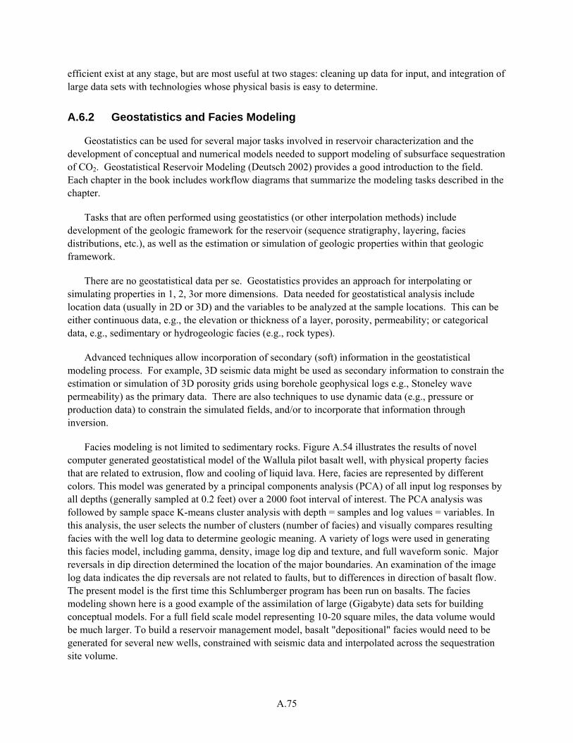
A.75

efficient exist at any stage, but are most useful at two stages: cleaning up data for input, and integration of large data sets with technologies whose physical basis is easy to determine.

A.6.2 Geostatistics and Facies Modeling

Geostatistics can be used for several major tasks involved in reservoir characterization and the development of conceptual and numerical models needed to support modeling of subsurface sequestration of CO2. Geostatistical Reservoir Modeling (Deutsch 2002) provides a good introduction to the field. Each chapter in the book includes workflow diagrams that summarize the modeling tasks described in the chapter.

Tasks that are often performed using geostatistics (or other interpolation methods) include development of the geologic framework for the reservoir (sequence stratigraphy, layering, facies distributions, etc.), as well as the estimation or simulation of geologic properties within that geologic framework.

There are no geostatistical data per se. Geostatistics provides an approach for interpolating or simulating properties in 1, 2, 3or more dimensions. Data needed for geostatistical analysis include location data (usually in 2D or 3D) and the variables to be analyzed at the sample locations. This can be either continuous data, e.g., the elevation or thickness of a layer, porosity, permeability; or categorical data, e.g., sedimentary or hydrogeologic facies (e.g., rock types).

Advanced techniques allow incorporation of secondary (soft) information in the geostatistical modeling process. For example, 3D seismic data might be used as secondary information to constrain the estimation or simulation of 3D porosity grids using borehole geophysical logs e.g., Stoneley wave permeability) as the primary data. There are also techniques to use dynamic data (e.g., pressure or production data) to constrain the simulated fields, and/or to incorporate that information through inversion.

Facies modeling is not limited to sedimentary rocks. Figure A.54 illustrates the results of novel computer generated geostatistical model of the Wallula pilot basalt well, with physical property facies that are related to extrusion, flow and cooling of liquid lava. Here, facies are represented by different colors. This model was generated by a principal components analysis (PCA) of all input log responses by all depths (generally sampled at 0.2 feet) over a 2000 foot interval of interest. The PCA analysis was followed by sample space K-means cluster analysis with depth = samples and log values = variables. In this analysis, the user selects the number of clusters (number of facies) and visually compares resulting facies with the well log data to determine geologic meaning. A variety of logs were used in generating this facies model, including gamma, density, image log dip and texture, and full waveform sonic. Major reversals in dip direction determined the location of the major boundaries. An examination of the image log data indicates the dip reversals are not related to faults, but to differences in direction of basalt flow. The present model is the first time this Schlumberger program has been run on basalts. The facies modeling shown here is a good example of the assimilation of large (Gigabyte) data sets for building conceptual models. For a full field scale model representing 10-20 square miles, the data volume would be much larger. To build a reservoir management model, basalt "depositional" facies would need to be generated for several new wells, constrained with seismic data and interpolated across the sequestration site volume.

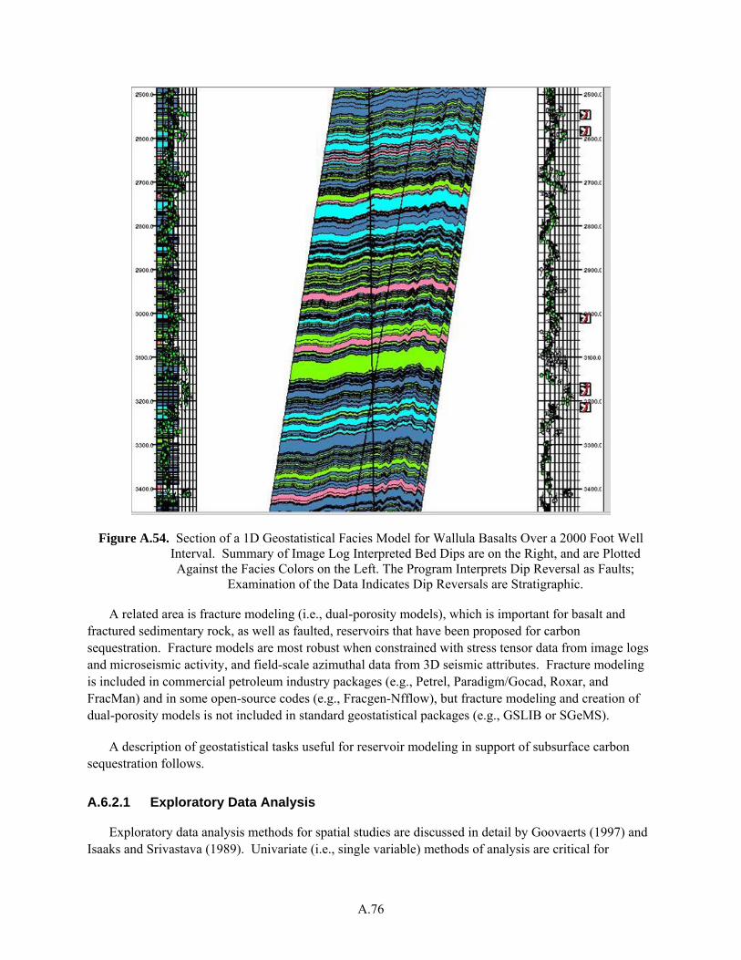
A.76

Figure A.54. Section of a 1D Geostatistical Facies Model for Wallula Basalts Over a 2000 Foot Well Interval. Summary of Image Log Interpreted Bed Dips are on the Right, and are Plotted Against the Facies Colors on the Left. The Program Interprets Dip Reversal as Faults;

Examination of the Data Indicates Dip Reversals are Stratigraphic.

A related area is fracture modeling (i.e., dual-porosity models), which is important for basalt and fractured sedimentary rock, as well as faulted, reservoirs that have been proposed for carbon sequestration. Fracture models are most robust when constrained with stress tensor data from image logs and microseismic activity, and field-scale azimuthal data from 3D seismic attributes. Fracture modeling is included in commercial petroleum industry packages (e.g., Petrel, Paradigm/Gocad, Roxar, and FracMan) and in some open-source codes (e.g., Fracgen-Nfflow), but fracture modeling and creation of dual-porosity models is not included in standard geostatistical packages (e.g., GSLIB or SGeMS).

A description of geostatistical tasks useful for reservoir modeling in support of subsurface carbon sequestration follows.

A.6.2.1 Exploratory Data Analysis

Exploratory data analysis methods for spatial studies are discussed in detail by Goovaerts (1997) and Isaaks and Srivastava (1989). Univariate (i.e., single variable) methods of analysis are critical for

A.77

examination of the underlying frequency distribution of the variable in question. The most common techniques for univariate analysis are generation of histograms, normal probability plots, and the calculation of univariate statistics (e.g., mean, median, standard deviation, and skewness). In those cases where a variable has a highly skewed distribution, it is usually necessary to work with a transform of the data that is more symmetric than the original distribution. Several transforms that are commonly used are described in the following section. Two widely used geostatistical software packages, GSLIB (Deutsch and Journel 1998) and SGEMS (Remy et al. 2009) will plot histograms and calculate univariate statistics; GSLIB also includes plotting of the normal probability plot.

One major aspect of exploratory data analysis is the calibration of primary (hard) and secondary (soft) data. This is often done through linear regression and scatter plots. For example, the collocated cokriging technique (Goovaerts 1997) uses the linear correlation coefficient to capture the relationship between the primary and secondary variables. In many cases, the lithofacies distributions will be mapped in the reservoir units, and properties within the lithofacies will be based on probability distributions of the properties within each lithofacies. These might be estimated by construction of box plots or histograms that show the frequency distribution of the variable of interest (e.g., porosity or permeability) for each lithofacies.

Identification of lithofacies is another important facet of exploratory data analysis. Several methods are commonly used for this purpose. John et al. (2008) recently proposed a relatively simple methodology to identify lithofacies based on partitioning of a single variable (e.g., acoustic impedance data from seismic or gamma ray well log data) into a set of subpopulations with normal distributions that best fit the global population distribution. In many cases however, a suite of borehole geophysical logs and core data are used to identify the lithofacies. In those cases, it is often necessary to perform an iterative process that first identifies the lithofacies for those locations where both core and log data are available, then use a different statistical method to identify those lithofacies for the larger population of samples where more limited data (e.g., only log or seismic data) are available. For example, Murray (1994) used cluster analysis to identify three lithofacies in the Muddy Sandstone in Amos Draw Field in the Powder River Basin of Wyoming. Examination of those lithofacies showed significant differences in porosity, permeability, and mineralogy that were related to variations in the depositional environment and diagenesis of the rocks. Discriminant function analysis was then used to identify those lithofacies in wells where only geophysical log data were available (Murray 1994). A wide assortment of multivariate analysis techniques are used for identification of lithofacies including cluster analysis (Murray 1994), discriminant function analysis (Murray 1994, Doveton 1994), fuzzy logic (Rezaei and Movahed 2009), and neural networks (Chang et al. 2000, Doveton 1994).

A.6.2.2 Reservoir Architecture

In most cases, the large scale architecture of the reservoir is implemented early in the development of the conceptual model (Deutsch 2002). This includes definition of the major geologic layers that are present, as well as any significant faults. Data for mapping the elevation and thickness of these major layers is a combination of well and/or seismic data and may be based on the sequence stratigraphic approach described in Section A.6.1. Interpolations of geologic layer and fault surfaces are typically generated using solid modeling software like EarthVision. Once the major architecture is defined, then lithofacies and continuous properties can be generated within that framework using geostatistics. All cells in some layers, e.g., secondary seals, may be assigned a single homogeneous value for hydrological

A.78

and geochemical properties needed for flow and transport modeling. Standard practice is to perform a geostatistical analysis for the spatial distribution of required properties for each major layer in which the properties are expected to show a significant amount of spatial variability (Deutsch 2002). The properties are normally simulated on a Cartesian grid of cells that partition the volume within each layer of the reservoir architecture. The definition and modeling of these cells can be stratigraphically and structurally complex. Deutsch (2002), in Chapter 3, Gridding Reservoir Layers, provides guidelines and strategies for defining the Cartesian grids used in geostatistical modeling.

A.6.2.3 Variogram Calculation and Modeling

The variogram is the basic tool used to develop models of spatial continuity for geostatistical modeling. Those models are needed because the subsurface is usually sparsely sampled and estimates (or simulated values) of geologic variables are needed on regular grids for flow and transport modeling. Geologists are intuitively aware that pairs of locations that are closer to one another will tend to have more similar values than pairs of locations that are farther apart. This tendency arises because many geologic processes, including the depositional and diagenetic processes that control porosity and permeability in the subsurface, exhibit a degree of spatial continuity. However, those processes are not so well behaved that an analytical function can be used to predict the values at unsampled locations. Instead, geostatistical methods, e.g., kriging or stochastic simulation are used to estimate or simulate values at unsampled locations (Deutsch 2002, Goovaerts 1997). In order to use those methods, mathematical estimates of the spatial continuity (or its inverse, the spatial variability) are needed as a function of distance; this model is used to calculate the weights assigned to nearby data points for estimation or simulation. The variogram is the tool typically used for this purpose (Deutsch 2002); it is used to calculate the variability of pairs of points of data as a function of the distance between pairs of points, shown as the red squares in Figure A.53. Because estimates of the spatial variability may be needed for distances other than those for which an empirical variogram value are available, a smooth continuous model (i.e., function) must be fit to the empirical variogram (Figure A.53).

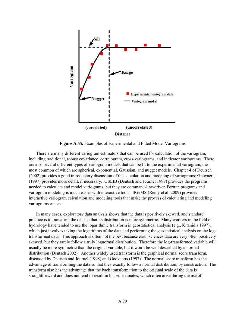
A.79

Figure A.55. Examples of Experimental and Fitted Model Variograms

There are many different variogram estimators that can be used for calculation of the variogram, including traditional, robust covariance, correlogram, cross-variograms, and indicator variograms. There are also several different types of variogram models that can be fit to the experimental variogram, the most common of which are spherical, exponential, Gaussian, and nugget models. Chapter 4 of Deutsch (2002) provides a good introductory discussion of the calculation and modeling of variograms; Goovaerts (1997) provides more detail, if necessary. GSLIB (Deutsch and Journel 1998) provides the programs needed to calculate and model variograms, but they are command-line-driven Fortran programs and variogram modeling is much easier with interactive tools. SGeMS (Remy et al. 2009) provides interactive variogram calculation and modeling tools that make the process of calculating and modeling variograms easier.

In many cases, exploratory data analysis shows that the data is positively skewed, and standard practice is to transform the data so that its distribution is more symmetric. Many workers in the field of hydrology have tended to use the logarithmic transform in geostatistical analysis (e.g., Kitanidis 1997), which just involves taking the logarithms of the data and performing the geostatistical analysis on the log-transformed data. This approach is often not the best because earth sciences data are very often positively skewed, but they rarely follow a truly lognormal distribution. Therefore the log-transformed variable will usually be more symmetric than the original variable, but it won’t be well described by a normal distribution (Deutsch 2002). Another widely used transform is the graphical normal score transform, discussed by Deutsch and Journel (1998) and Goovaerts (1997). The normal score transform has the advantage of transforming the data so that they exactly follow a normal distribution, by construction. The transform also has the advantage that the back transformation to the original scale of the data is straightforward and does not tend to result in biased estimates, which often arise during the use of

A.80

lognormal geostatistics (Goovaerts 1997). Both GSLIB and SGeMS include software to perform the forward and backward normal score transform of data.

A.6.2.4 Geostatistical Kriging and Simulation

Kriging is a family of generalized least-squares regression algorithms that can be used to estimate the value of categorical variables (e.g., lithofacies) or continuous variables (e.g., porosity, permeability, or the concentration of a reactive mineral) at unsampled locations (Goovaerts 1997). For continuous variables, kriging provides an estimate of the mean and variance of the variable of interest, usually on a regular Cartesian grid developed over the area or volume of interest. Given the least squares optimization algorithms used for its calculation, the kriging estimate has certain optimal properties, as it is constructed to be the best linear unbiased estimator that minimizes the variance of the prediction error. The kriging estimate and variance at each grid node is a weighted linear combination of the nearby data, where the weights are determined by solving a set of linear equations known as the normal equations. The weights assigned to the nearby data depend on the variogram model fit to the variable. There are several varieties of kriging that have been developed for continuous variables, see Goovaerts (1997) or Deutsch (2002) for details. For categorical variables like lithofacies, a variety of kriging known as indicator kriging can be used to calculate the probability that each lithofacies is present at an unsampled location.

Grids of kriged estimates of permeability and porosity are rarely used directly in reservoir modeling, because, like most linear regression estimates, they are highly smoothed versions of the data that do not have the same spatial variability as the original data. For that reason, most reservoir modeling is done with stochastic simulations of the required properties. Kriging forms the basis for most stochastic simulation algorithms. The basic approach for sequential stochastic simulation uses kriging to estimate the cumulative distribution function (CDF) for the variable for a randomly selected node of the grid (Figure A.54). A simulated value is then chosen at random from the CDF for that grid node, and subsequently used as data for simulation of other nodes. By visiting each location in a random sequence and each time drawing a value from the CDF determined by kriging the nearby data, a single realization is generated (Figure A.54). Another realization can be generated by repeating the process, but taking a different random path through the sequence of grid nodes. Each realization generated in this way will reproduce the existing data, as well as the variogram model (Goovaerts 1997). It will not exhibit the type of smoothing exhibited by a kriged grid. Each realization can be used as an input to a flow and transport model, and because large numbers of equally probable realizations are easily generated, the sequential simulation method is a natural basis for estimating the uncertainty associated with flow and transport predictions based on a particular conceptual model.

Using different forms of kriging, it is possible to use the sequential simulation technique to generate realizations of either categorical or continuous properties. The next section describes several alternative methods for generating realizations of lithofacies and other categorical properties.

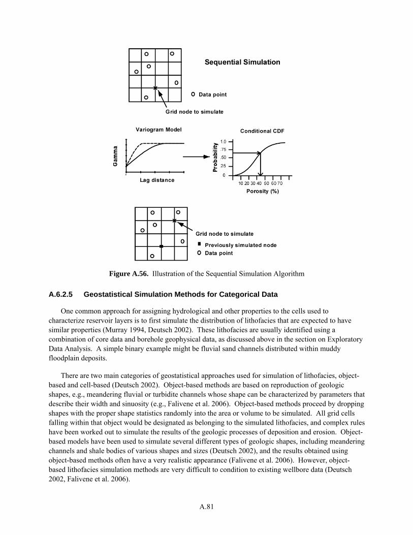
A.81

Figure A.56. Illustration of the Sequential Simulation Algorithm

A.6.2.5 Geostatistical Simulation Methods for Categorical Data

One common approach for assigning hydrological and other properties to the cells used to characterize reservoir layers is to first simulate the distribution of lithofacies that are expected to have similar properties (Murray 1994, Deutsch 2002). These lithofacies are usually identified using a combination of core data and borehole geophysical data, as discussed above in the section on Exploratory Data Analysis. A simple binary example might be fluvial sand channels distributed within muddy floodplain deposits.

There are two main categories of geostatistical approaches used for simulation of lithofacies, object-based and cell-based (Deutsch 2002). Object-based methods are based on reproduction of geologic shapes, e.g., meandering fluvial or turbidite channels whose shape can be characterized by parameters that describe their width and sinuosity (e.g., Falivene et al. 2006). Object-based methods proceed by dropping shapes with the proper shape statistics randomly into the area or volume to be simulated. All grid cells falling within that object would be designated as belonging to the simulated lithofacies, and complex rules have been worked out to simulate the results of the geologic processes of deposition and erosion. Object-based models have been used to simulate several different types of geologic shapes, including meandering channels and shale bodies of various shapes and sizes (Deutsch 2002), and the results obtained using object-based methods often have a very realistic appearance (Falivene et al. 2006). However, object-based lithofacies simulation methods are very difficult to condition to existing wellbore data (Deutsch 2002, Falivene et al. 2006).

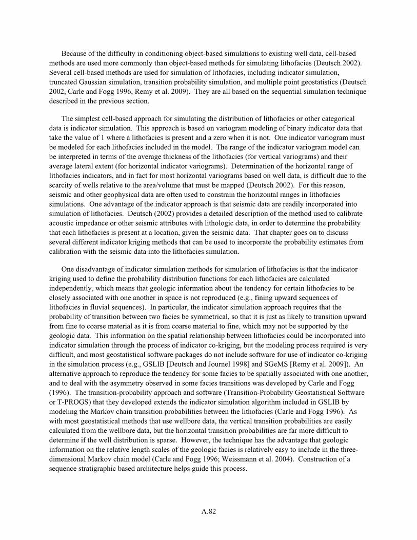
A.82

Because of the difficulty in conditioning object-based simulations to existing well data, cell-based methods are used more commonly than object-based methods for simulating lithofacies (Deutsch 2002). Several cell-based methods are used for simulation of lithofacies, including indicator simulation, truncated Gaussian simulation, transition probability simulation, and multiple point geostatistics (Deutsch 2002, Carle and Fogg 1996, Remy et al. 2009). They are all based on the sequential simulation technique described in the previous section.

The simplest cell-based approach for simulating the distribution of lithofacies or other categorical data is indicator simulation. This approach is based on variogram modeling of binary indicator data that take the value of 1 where a lithofacies is present and a zero when it is not. One indicator variogram must be modeled for each lithofacies included in the model. The range of the indicator variogram model can be interpreted in terms of the average thickness of the lithofacies (for vertical variograms) and their average lateral extent (for horizontal indicator variograms). Determination of the horizontal range of lithofacies indicators, and in fact for most horizontal variograms based on well data, is difficult due to the scarcity of wells relative to the area/volume that must be mapped (Deutsch 2002). For this reason, seismic and other geophysical data are often used to constrain the horizontal ranges in lithofacies simulations. One advantage of the indicator approach is that seismic data are readily incorporated into simulation of lithofacies. Deutsch (2002) provides a detailed description of the method used to calibrate acoustic impedance or other seismic attributes with lithologic data, in order to determine the probability that each lithofacies is present at a location, given the seismic data. That chapter goes on to discuss several different indicator kriging methods that can be used to incorporate the probability estimates from calibration with the seismic data into the lithofacies simulation.

One disadvantage of indicator simulation methods for simulation of lithofacies is that the indicator kriging used to define the probability distribution functions for each lithofacies are calculated independently, which means that geologic information about the tendency for certain lithofacies to be closely associated with one another in space is not reproduced (e.g., fining upward sequences of lithofacies in fluvial sequences). In particular, the indicator simulation approach requires that the probability of transition between two facies be symmetrical, so that it is just as likely to transition upward from fine to coarse material as it is from coarse material to fine, which may not be supported by the geologic data. This information on the spatial relationship between lithofacies could be incorporated into indicator simulation through the process of indicator co-kriging, but the modeling process required is very difficult, and most geostatistical software packages do not include software for use of indicator co-kriging in the simulation process (e.g., GSLIB [Deutsch and Journel 1998] and SGeMS [Remy et al. 2009]). An alternative approach to reproduce the tendency for some facies to be spatially associated with one another, and to deal with the asymmetry observed in some facies transitions was developed by Carle and Fogg (1996). The transition-probability approach and software (Transition-Probability Geostatistical Software or T-PROGS) that they developed extends the indicator simulation algorithm included in GSLIB by modeling the Markov chain transition probabilities between the lithofacies (Carle and Fogg 1996). As with most geostatistical methods that use wellbore data, the vertical transition probabilities are easily calculated from the wellbore data, but the horizontal transition probabilities are far more difficult to determine if the well distribution is sparse. However, the technique has the advantage that geologic information on the relative length scales of the geologic facies is relatively easy to include in the three-dimensional Markov chain model (Carle and Fogg 1996; Weissmann et al. 2004). Construction of a sequence stratigraphic based architecture helps guide this process.

A.83

While the Markov-chain based approach developed in T-PROGS does a better job of reproducing important geologic characteristics than indicator simulation, it still has a significant problem, one that it shares with variogram-based methods. Because those methods rely on reproduction of variogram and transition probability models that operate on pairs of points at a time, they normally cannot reproduce geologic features with a significant amount of curvature, unless the data distribution is very dense. As mentioned above, the ability to reproduce fluvial channels with significant curvature is one of the advantages of object-based simulation methods, though this advantage is outweighed by the difficulty in reproducing existing wellbore data. Multiple-point simulation, a relatively recent addition to the geostatistical toolbox, appears to provide a reasonable compromise, allowing direct reproduction of existing wellbore data, plus the ability to reproduce geologic shapes with complex curvature (Falivene et al. 2006). The multiple-point geostatistical method operates by identifying spatial distributions of categorical data like lithofacies by scanning a training image using a set of templates. For example Figure A.55 shows all possible arrangements of a square four-point template for a binary system with two categories (Boisvert et al. 2008). For this template, scanning of a training image would produce statistics on how often each of the 16 possible configurations arose, which provides an estimate of the multiple-point density function (MPDF) for that particular training image and template. Traditional variogram (i.e., 2-point) simulation methods generate realizations that honor the data and a variogram model, which is a 2-point statistic; multiple-point geostatistical simulation on the other hand aims to reproduce the existing data and the multiple-point structures present in the training image (Remy et al. 2009).

Figure A.57. Diagram Showing the 16 Possible Patterns of Distribution of 2 Lithofacies for a Four-Cell Scanning Template (Boisvert et al. 2008)

Figure A.58 provides an example from Strebelle (2002) showing two realizations, one generated using multiple-point geostatistics, and one generated using indicator geostatistics. While both honor the conditioning data and have the same variogram, the east-west connectivity of the multiple-point realization and reproduction of the curvilinear shapes found in the training image is much greater than that possible with the indicator method. The SGeMS package includes two different implementations of

A.84

multiple-point simulation (snesim and filtersim), as well as a utility (TIgenerator) that can be used to create training images with specific geologic shapes and interactions (Remy et al. 2009).

A.6.2.6 Simulation Methods for Continuous Data

There are many types of continuous data for which numerical grids may need to be generated in carbon sequestration studies. Porosity and permeability are the most common, and are always needed for flow and transport modeling studies. However, reactive transport modeling of carbon sequestration would require additional grids of properties expected to influence reactive transport. These might include sediment properties such as mineral concentrations, bulk rock chemical analyses, the results of chemical extractions of subsurface sediments, or proxies for geochemical reactivity such as measurements of surface area for sediment samples.

Figure A.58. Illustrations of 2 Facies Categorical Realizations Generated using Multiple-Point Geostatistics (A) and Indicator Geostatistics (B) (Strebelle 2002)

(Note the more strongly connected facies that are generated using the multi-point method.)

Two geostatistical methods are commonly used for simulation of continuous data, sequential Gaussian simulation and sequential indicator simulation. Sequential Gaussian simulation is typically the easiest and most straightforward method to apply and is the most widely used method in reservoir modeling (Deutsch 2002). The main requirement for application of the method is modeling a single variogram, the variogram of the normal score transform of the data. Secondary data can be incorporated through several algorithms. A common approach is to first simulate the distribution of lithofacies using one of the methods described in the previous section. Then, the method of locally varying means (Goovaerts 1997) can be used to simulate a continuous variable, e.g., porosity, conditioned on a previously generated simulation of the lithofacies distribution. A calibration is performed to identify the mean value of the continuous variable for each lithofacies class. An alternative approach for incorporating secondary data is to use the collocated cokriging algorithm (Goovaerts 1997). In that algorithm, we calculate the correlation coefficient between the normal scores of the primary and secondary data. This algorithm is often used to simulate permeability conditional to previously generated simulations of porosity (Deutsch 2002), because porosity data are usually more numerous and porosity is more easily estimated from seismic and borehole log data than permeability. Thus we can use a stepwise

A.85

approach to the simulation of permeability, first simulating the distribution of lithofacies, then simulating the porosity conditional to the lithofacies simulations, and finally simulating the permeability conditioned on the porosity simulations.

In order for the use of sequential Gaussian simulation to be appropriate, the variable in question should have a multivariate Gaussian spatial distribution. Usually, this assumption cannot be tested rigorously because of a lack of sufficient data, but it is possible to test if the bivariate spatial distribution appears to be Gaussian (Goovaerts 1997). This test can be revealing because it involves comparison of the indicator variograms for a series of thresholds to the variogram models that would be expected if the variable has a bivariate Gaussian spatial distribution. The most revealing part of this test is whether or not the tails of the distribution, e.g., the extremely high or low values of a permeability distribution, have a higher degree of spatial correlation than would be predicted for a Gaussian variable. Highly correlated low or high permeability values are occasionally found during reservoir characterization, and if the degree of correlation is significantly higher than predicted, then the use of sequential Gaussian simulation may not be justified (Goovaerts 1997). If that occurs, then sequential indicator simulation should be considered. It is worth noting that the stepwise approach outlined above may take care of the problem if the highly correlated zones of high or low permeability are associated with particular lithofacies, with Gaussian behavior within the lithofacies (Deutsch 2002).

Sequential indicator simulation was discussed in the previous section for simulation of categorical data, e.g., lithofacies. It can also be used for simulation of continuous data, such as permeability. Continuous variables are transformed to indicator variables by defining a series of thresholds, that capture the shape of the cumulative histogram of the variable. Normally, between 5 and 11 thresholds are used, with the 9 quantiles of the data being a common choice (Deutsch 2002). For a given location, the data, e.g., a permeability values, are transformed to a series of binary indicators, one for each threshold. These hard binary indicators take the value of 1 if the permeability value at that location is less than a given threshold, and zero if it exceeds the threshold. Variograms are calculated and modeled for each threshold, providing a separate model of spatial correlation of each threshold. This can allow the development of spatial models with much greater correlation for low or high permeability thresholds, where a Gaussian model assumes that the greatest spatial correlation is for the mean of the distribution (Goovaerts 1997). Indicator kriging can then be used at unsampled locations to estimate the probability that each threshold is exceeded. An independent kriging is performed for each threshold, providing an estimate of the cumulative histogram of the variable at each unsampled location. For sequential indicator simulation, once the kriging of each threshold is completed for a grid node being simulated, a value is drawn from that cumulative histogram and used for the simulation of all subsequent nodes. The indicator formalism is very flexible, allowing for encoding of secondary (soft) data (Deutsch 2002). This requires a calibration of the secondary variable with the indicator thresholds. One method of calibration and coding results in the assignment of soft probability values for each threshold that fall between 0 and 1, that capture the probability that the variable of interest is less than a given threshold for an observed value of the secondary variable. Those soft probability values can then be directly incorporated in the sequential indicator simulation and allow for assimilation of hard and soft data.

The indicator approach for simulation of continuous variables is more difficult to apply, so unless the data exhibit a strongly non-Gaussian spatial distribution, sequential Gaussian simulation will be the preferred approach for simulation of continuous variables (Deutsch 2002, Goovaerts 1997). The use of sequential Gaussian simulation is more likely to be effective when the approach is combined with the use of lithofacies that capture most of the variability in the reservoir properties of interest.

A.86

A.7 Upscaling

Upscaling refers to the mapping or averaging of data or parameters determined at one scale to larger scales. Upscaling has a long history in the fields of petroleum engineering and hydrology (Renard and de Marsily 1997; Durlofsky 2002). For scalar variables, such as porosity or mineral volume fractions, the method of volume averaging is required to conserve mass and volume within the domains of interest. For tensor variables, such as permeability and relative permeability, fast approximate methods include weighted combinations of arithmetic and harmonic means (Fleckenstein and Fogg 2008, Li et al. 2001, Malik and Lake 1997), renormalization methods (Hinrichsen et al. 1993, King 1989), and continuous-time random walk particle tracking (McCarthy 1995).

More accurate and computationally demanding methods for upscaling permeability include directly solving the flow equations at the fine scale on subdomains of the larger field (He et al. 2002; Peszynska et al. 2002). All of the more rigorous permeability upscaling approaches can be problematic owing to boundary effects. Boundary conditions for upscaling methods based on directly solving flow equations are usually a combination of no-flow and periodic or no-flow and fixed pressure (Dirichlet) conditions. As noted by Renard and de Marsily (1997) the upscaled result is dependent on the boundary conditions which cannot be known a priori. For this reason, and also owing to uncertainty associated with sparsely sampled domains, some of the fast approximate methods can be attractive.

We have developed several codes for upscaling both scalar and tensor variables. The first code, called UPSCALE3D.F90, uses volume averaging to upscale (or downscale) scalar variables such as porosity, and the geometric mean of the so-called Cardwell and Parsons bounds (Cardwell and Parsons, 1945) to estimate upscaled values of the principal components of an effective permeability tensor. The combination of these methods yields exact results for all cases in which exact results are known and the code works for any rectilinear Cartesian grids with uniform or nonuniform spacings. This code is used routinely by researchers in the Hydrology Group at PNNL to upscale results obtained on uniform and relatively fine or high-resolution geostatistical model grids to non-uniform and generally coarser model grids used by the STOMP simulator (Oostrom et al. 2006, Williams et al. 2008).

Another upscaling code that we have developed is called CTRW4K.F90. This code performs permeability upscaling using a continuous-time random walk particle tracking method (McCarthy 1995). This method produces more accurate results in most cases than renormalization methods and yields results that are almost as accurate as direct numerical solutions to the single-phase flow equation. The CTRW4K code will generate more accurate results than the UPSCALE3D code for fields that have strongly connected features that result in preferential flow paths.

Another upscaling approach that is commonly used requires the use of field pump test data and core- or well-log-based measurements of porosity and permeability for the borehole. The latter are used to estimate correlation lengths that are used to generate spatially-correlated random fields conditioned on the borehole core or well log data. A flow and transport simulator such as STOMP is then used to simulate the pump test using the spatially correlated random fields. Simulation results are then compared to the field-scale pump test results and horizontal permeabilities are scaled up or down, as needed, until an adequate match is obtained.

A.87

Petrel™ handles the upscaling problem in several different ways; by upscaling well log data, by simple averaging, or by flow-based tensor upscaling. For upscaling well logs cross sections are constructed and logging intervals are averaged vertically through an interactive process. The upscaled well log values are then used for conditioning in geostatistical stochastic simulation. This approach is very simple and may not lead to very accurate results compared to some other methods, but this would depend on the types of core and well log data that are available and on the size and complexity of the site. The simple averaging approach used in Petrel is probably comparable to that implemented in the UPSCALE3D program noted above. The flow-based tensor upscaling requires the use of a flow simulator. Petrel also interfaces with the Eclipse simulator and has an optional module for streamline simulation. Depending on how the streamline simulation is implemented, it could potentially be used as part of a permeability upscaling procedure.

Upscaling of reaction kinetics is a very challenging problem. It is well known that reaction rates measured in the laboratory under well-mixed conditions are much faster than those that occur in natural field settings. This has been attributed to a variety of factors including armoring of surfaces in the field such that initially reactive surfaces become coated by reaction products that limit the rates of further reactions, and rate-limited mass transfer effects. Reaction rates in the field are confounded by physical and geochemical heterogeneities and mass transfer effects such as slow diffusion into and out of immobile pore regions. Some of these issues have been addressed through the development of multi-continuum models of mass transfer and reaction processes (Lichtner and Kang 2007), network flow modeling (Li et al. 2006), and mixed Lagrangian and Eulerian methods (Tartakovsky et al. 2008). However many of these models are difficult to parameterize using independent measurements, and the development of effective methods for upscaling laboratory-observed mineral reaction kinetics to parameterize field-scale reactive transport models still remains somewhat elusive. This topic is being addressed by several other projects on PNNL’s Carbon Sequestration Initiative using both experimental and numerical methods.

A.8 Special Needs for CO2 Sequestration

Characterization, modeling, and monitoring of CO2 sequestration sites present several challenges. One of the most important of these is the need to characterize the impact of CO2 injection on formation properties and on fault and fracture characteristics. There are several technologies that could aid in both characterization and monitoring. Some of these are listed below:

• Pulsed Neutron Sigma measurements represent one of the most promising areas of research and data assimilation for quantifying saturations and calibrating VSP, cross-well and surface-based seismic signatures. Wireline log derived Stoneley wave permeability represents one of the most robust and promising new means of building "permeability" facies and of calibrating seismic frequency-dependent attributes that are linked to permeability.

• Geochemical log generation and analysis needs to be adapted to CO2 sequestration needs. Some of the adaptations may be relatively easy: development of simple software to cross-plot various logs to provide flags for reactive geochemistry; and software for incorporating reactive geochemistry into existing facies modeling software.

A.88

• Data assimilation and inversion technologies for large data sets associated with seismic data and a variety of other data types including: electrical resistivity tomography micro gravity, microseismic, and a variety of remotely sensed data.

• Development and calibration of volumetric P-wave and multicomponent seismic attributes with changes in CO2 saturations. This is an emerging field of research for carbon sequestration.

• Improved and higher-resolution monitoring of subsurface CO2 plume movement and dynamics. Resolving data collected at various scales; scale-dependent interpretation of data.

• Robust algorithms for upscaling properties and parameters (particularly reaction rates) from core- and log-based measurements to numerical model grid blocks.

• Petrophysical and geomechanical catalogues of lab-scale properties, including generation of new laboratory measurements relevant to CO2. These include but are not limited to equations of state; log, geomechanical, and seismic responses to changes in saturation of CO2 , and brine, rock/mineral compositions.

• Specific studies focused on improved data collection, processing and interpretation, to produce improved quantification of CO2 properties (saturation, pore pressure, etc), as well as far field pressures and earth stresses.

• Development of integration technologies for comparing operational monitoring data with model data for verification of subsurface CO2 volumes, plume movement and early warning of potential leakage.

 

A.89

A.9 References Adams JAS, and CE Weaver. 1958. “Thorium to Uranium Ratios as Indicators of Sedimentary Processes – Example of Concept of Geochemical Facies.” Am. Assoc. Petrol. Geol. Bull. 42(2):387-430.

American Petroleum Institute. 1998. Recommended Practices for Core Analysis. API RP 40, American Petroleum Institute, Washington, DC.

Archie GE. 1942. “The Electrical Resistivity Log as an Aid in Determining Some Reservoir Characteristics.” Petroleum Transactions, AIME, 146:54-62.

Arts, R, O Eiken, A Chadwick, P Zweigel, B van der Meer, and B. Zinszner, 2004. "Monitoring of CO2 injected at Sleipner using time-lapse seismic data". Energy 29: 1383–1392. Barton, CA, MD Zoback, and D Moos. 1995. "Fluid flow along potentially active faults in crystalline rock." Geology 23(8): 683–686.

Beaubouef RT, C Rossen, FB Zelt, M D Sullivan, DC Mohrig, and DC Jennette. 1999. Field guide for AAPG Hedberg Field Research Conference: deep-water sandstones, Brushy Canyon Formation, West Texas, April 15-20, 1999. The American Association of Petroleum Geologists, Tulsa, Oklahoma.

Blumentritt CH, KJ Marfurt, and EC Sullivan. 2006. “Volume based curvature computations illuminate fracture orientations, lower Paleozoic, Central Basin platform, West Texas.” Geophysics 71(5):B159-B166.

Blumentritt CH, KJ Marfurt, and M Murphy. 2007. “Constraining fracture systems with seismic curvature attributes: Teapot Dome, Wyoming.” Am. Assoc. Petrol. Geol Convention.

Boisvert, JB, MJ Pyrcz, and CV Deutsch. 2007, "Multiple-Point Statistics for Training Image Selection." Natural Resources Research 16:313-21.

Cardiff M, and PK Kitanidis. In Press. “Bayesian Inversion for Facies Detection: An Extensible Level Set Framework.” Water Resour Res.

Cardwell WT and RL Parsons. 1945. "Average Permeabilities of Heterogeneous Oil Sands." Trans. Am. Inst. Mining Met. Pet. Eng. 160:34-42.

Carle SF and GE Fogg. 1996. "Transition Probability-Based Indicator Geostatistics." Mathematical Geology 28(4):453-76.

Castagna, J P, S Sun, and RW Siegfried. 2003. "Instantaneous spectral analysis: Detection of low frequency shadows associated with hydrocarbons". The Leading Edge, 22, (2): 120-127.

Chadwick RA, D Noy, R Arts, and O Eiken. 2009. “Latest time lapse seismic data from Sleipner yields new insights into CO2 plume development.” Energy Procedia 1(1):2103-2110.

Chang C, MD Zoback, and A Khaksar. 2006. “Empirical correlations between rock strength and physical properties in sedimentary rocks.” J. Petrol. Sci. Eng. 51(3-4):223-237.

A.90

Chang HC, SR Durrans, DC Kopaska-Merkel, HC Chen. 2000, "Lithofacies Identification Using Multiple Adaptive Resonance Theory Neural Networks and Group Decision Expert System." Computers & Geosciences 26(5):591-601.

Chiaramonte L, MD Zoback, J Friedmann, and V Stamp. 2008. “Seal integrity and feasibility of CO2 sequestration in the Teapot Dome EOR pilot: geomechanical site characterization.” Environ. Geol. 54(8):1667-1675.

Chopra, S, and K J Marfurt. 2007. Seismic attributes for prospect identification and reservoir characterization. Society of Exploration Geophysicists, Tulsa, OK, 456 p.

Chopra S and KJ Marfurt. 2005. “Seismic Attributes- A historical perspective.” Geophysics 70, 3SO doi:10.1190/1.2098670.

Clavier C, G Coates, and J Dumanoir. 1984. “The Theoretical and Experimental Bases for the Dual-Water Model for the Interpretation of Shaly Sands.” Soc Petrol Engin J 24(2):153-169.

Coughlin P. 1982. Reservoir Quality and Fluid Sensitivity Analysis of Samples from the Tensleep “Zone A” Sandstone in the Teapot Dome Field, Natrona County, Wyoming. D-310, AGAT Consultants, for Lawrence-Allison and Associates West, Inc., Denver, Colorado.

Curtis, A, P Gerstoft, H Sato, and R Snieder. 2006. "Seismic interferometry—turning noise into signal". The Leading Edge. 25 (9): 1082-1092.

Daily W, A Ramirez, A Binley, and D LeBreque. 2008. “Electrical resistance tomography.” The Leading Edge 23(5):438-442.

Deutsch, CV. 2002. Geostatistical Reservoir Modeling. Oxford University Press, New York, New York.

Deutsch, CV and AG Journel. 1998. GSLIB: Geostatistical Software Library and User's Guide. 2nd. Ed. Oxford University Press, New York, New York.

Dou Q, Y Sun, and C Sullivan. 2009. “Collapsed-Paleocave Systems in the Permian San Andres Formation, Central Basin Platform, West Texas, Revealed by Integrated Seismic Characterization.” AAPG Search and Discovery Article #90090, AAPG Annual Convention and Exhibition, Denver, Colorado, June 7-10, 2009.

Doveton JH. 1982. The Kansas State Log Analysis Course. Kansas Geological Survey, Lawrence, Kansas.

Doveton JH. 1994. Geologic Log Analysis using Computer Methods. American Association of Petroleum Geologists, Tulsa, Oklahoma.

Dubois MK, AP Byrnes, S Bhattacharya, GC Bohling, JH Doveton, and RE Barba. 2006. Hugoton Asset Management Project (HAMP): Hugoton Geomodel Final Report. Kansas Geological Survey, Lawrence, Kansas.

Durlofsky LJ. 2002. Upscaling of geological models for reservoir simulation: Issues and approaches. Computational Geosciences 6:1-4

A.91

Ellis DV and JM Singer. 2007. Well Logging for Earth Scientists. 2nd Ed. Springer-Verlag, New York, New York.

EPA. 2008. Geologic CO2 Sequestration Technology and Cost Analysis, Technical Support Document. EPA 816-B-08-009, US Environmental Protection Agency, Washington, D.C.

Falivene O, P Arbués, A Gardiner, G Pickup, JA Muñoz, and L Cabrera. 2006. "Best Practice Stochastic Facies Modeling from a Channel-Fill Turbidite Sandstone Analog (the Quarry Outcrop, Eocene Ainsa Basin, Northeast Spain)." American Association of Petroleum Geologists Bulletin 90(7):1003-1029.

Fleckenstein JH and GE Fogg. 2008. “Efficient upscaling of hydraulic conductivity in heterogeneous alluvial aquifers.” Hydrogeology Journal 16(7):1239-1250.

Fu D, EC Sullivan, and KJ Marfurt. 2006. “Rock property and seismic attribute analysis of a chert reservoir in the Devonian Thirtyone Formation, West Texas.” Geophysics 71(5), B151–B158.

Goloshubin G and D Silin. 2006. “Frequency-dependent reflection from a permeable boundary in a fractured reservoir.” 76th Annual SEG Meeting, New Orleans, Lousiana.

Goloshubin, G M, VA Korneev, and T.V. Daley. 2001. "Seismic low-frequency effects in gas reservoir monitoring VSP data", Expanded Abstract Annual SEG Meeting.

Goovaerts P. 1997. Geostatistics for Natural Resources Evaluation. Oxford University Press, New York, New York.

Gysen M, C Mayer, and KH Hashmy. 1987. “A new approach to log analysis involving simultaneous optimization of unknowns and zoned parameters.” 11th Formation Evaluation Symposium, Canadian Well Logging Society.

Hardage B. 2009. Improving the Monitoring, Verification, and Accounting of CO2 Sequestered in Geologic Systems with Multicomponent Seismic Technology and Rock Physics Modeling. Narrative, DOE Funded Grant DE-FOA0000023, U.S. Department of Energy, Washington, DC.

Hardage B, D Sava, R Remington, and M DeAngelo. 2008. Rock Physics and the Case for Multicomponent Seismic Data. Search and Discovery Article #40273. Accessible at http://www.searchanddiscovery.com/documents/2008/08006hardage0108/index.

Harris PM and AH Saller. 1999. “Subsurface expression of the Capitan depositional system and implications for hydrocarbon reservoirs, northeastern Delaware Basin.” In Geologic Framework of the Capitan Reef, eds. AH Saller, PM Harris, BL Kirkland, and SJ Mazzullo. SEPM Special Publication 65, Society for Sedimentary Geology, Tulsa, Oklahoma.

Hassan M, A Hossin, and A Combaz. 1976. “Fundamentals of the differential gamma-ray log - Interpretation Technique.” SPWLA 17th Annual Logging Symposium.

He C, MG Edwards, LJ Durlofsky. 2002. Numerical calculation of equivalent cell permeability tensors for general quadrilateral control volumes. Computational Geosciences 6:29-47.

Herron MM. 1988. “Geochemical Classification of Terrigenous Sands and Shales from Core or Log Data.” J. Sed. Res. 58:820-829.

A.92

Herron MM and SL Herron. 1990. “Geological applications of geochemical well logging.” Geological Society, London, Special Publication 48:165-175. DOI: 10.1144/GSL.SP.1990.048.01.14.

Hertzog R, L Colson, M O’Brien, H Scott, D McKeon, P Wraight, J Grau, D Ellis, J Schweitzer, and M Herron. 1989. “Geochemical Logging with Spectrometry Tools.” Soc. Petro. Engin. 4(2):153-162.

Hecht CA, C Bonsch, and E Bauch. 2005. “Relations of Rock Structure and Composition to Petrophysical and Geomechanical Rock Properties: Examples from Permocarboniferous Red-Beds.” Rock Mech. Rock Engng. 38(3):197–216.

Hinrichsen EI, A Aharony, J Feder, A Hansen, T Jossang. 1993. “A fast algorithm for estimating large-scale permeabilites of correlated anisotropic media.” Transport in Porous Media. 12(1):55-72.

Hovorka, SD, D Collins, S Benson, L Myer, C Bryer, and K Cohen. 2005. “Update on the Frio Brine Pilot: Eight months after injection.” Presented at the National Energy Technology Laboratory Fourth Annual Conference on Carbon Capture and Sequestration, Alexandria, Virginia, May 2-5, 2005. Gulf Coast Carbon Center Digital Publication Series #05-04i.

Hurley C. 1986. Final Report, Special Core Analysis, Tensleep Reservoir. RFP No. 85-09, Terra Tek Research, Salt Lake City, Utah.

Isaaks, EH and RM Srivastava. 1989. An Introduction to Applied Geostatistics. Oxford University Press, New York, New York.

James H. 2009. “Visualizing 3D features in 3D seismic data.” First Break. 27(3):57-62.

John, AK, LW Lake, C Torres-Verdin, and S Srinivasan. 2008. "Seismic Facies Identification and Classification Using Simple Statistics." SPE Reservoir Evaluation & Engineering 11(6):984-90.

Jordan PD, CM Oldenburg, and JP Nocot. 2008. “Characterizing fault-plume intersection probability for geologic carbon sequestration risk assessment." Energy Procedia, GHGT9 Conference, Washington, DC, November 16-20, 2008.

Kerans C. 2002. Styles of rudist buildup development along the northern margin of the Maverick Basin, Pecos River Canyon, Southwest Texas. Gulf Coast Association of Geological Societies Transactions, 52, pp 501-516.

Kitanidis PK. 1997. Introduction to Geostatistics: Applications in Hydrogeology. Cambridge University Press, New York, New York.

King PR. 1987. “The use of renormalization for calculating effective permeability.” Transport in Porous Media. 4(1):37-58.

Korneev, VA, GM Goloshubin, TV Daley, and DB Silin. 2004. "Seismic low-frequency effects in monitoring of fluid-saturated reservoirs". Geophysics, 69 N2:522-532

Leetaru H. 2009. “Seismic interpretation of the Mattoon P-wave data.” Unpublished site characterization support materials for the Mattoon FutureGen site.

Li D, B Beckner, and A Kumar. 2001. A new efficient averaging technique for scaleup of multimillion cell geologic models. SPE Reservoir Evaluation and Engineering. 4(4):297-307.

A.93

Li L, CA Peters, and MA Celia. 2006. “Upscaling geochemical reaction rates using pore-scale network modeling.” Adv Water Resour. 29(9):1351-1370.

Lichtner PC and Q Kang. 2007. “Upscaling pore-scale reactive transport equations using a multiscale continuum formulation.” Water Resour. Res. 43(12):W12S15 1-W12S15.19.

Malik MA and LW Lake. 1997. “A practical approach to scaling-up permeability and relative permeabilities in heterogeneous permeable media.” SPE Western Regional Meeting, 25-27 June 1997, Long Beach, California.

McCarthy JF. 1995. Comparison of fast algorithms for estimating large-scale permeabilities of heterogenous porous media. Transport in Porous Media 19(2):123-137.

McGrail BP, C Sullivan, CL Davidson, WE Fallon, ME Kelley, MD White, SK Wurstner, BN Bjornstad, JL Downs, CJ Murray, CW Stewart, KM Krupka, DH Bacon, PE Jagucki, PD Thorne, GE Hammond, R Mackley, and ML Stewart. 2006a. Environmental Information Volume: Tuscola, Illinois . PNWD-3765, Battelle,Pacific Northwest Division, Richland, Washington.

McGrail BP, C Sullivan, CL Davidson, WE Fallon, ME Kelley, MD White, SK Wurstner, BN Bjornstad, JL Downs, CJ Murray, CW Stewart, KM Krupka, DH Bacon, PE Jagucki, PD Thorne, GE Hammond, R Mackley, and ML Stewart. 2006b. Environmental Information Volume: Heart of Brazos, Texas . PNWD-3767, Battelle, Pacific Northwest Division, Richland, Washington.

McGrail BP, C Sullivan, CL Davidson, WE Fallon, ME Kelley, MD White, SK Wurstner, BN Bjornstad, JL Downs, CJ Murray, CW Stewart, KM Krupka, DH Bacon, PE Jagucki, PD Thorne, GE Hammond, R Mackley, and ML Stewart. 2006c. Environmental Information Volume: Mattoon, Illinois . PNWD-3768, Battelle, Pacific Northwest Division, Richland, Washington.

McGrail BP, C Sullivan, CL Davidson, WE Fallon, ME Kelley, MD White, SK Wurstner, BN Bjornstad, JL Downs, CJ Murray, CW Stewart, KM Krupka, DH Bacon, PE Jagucki, PD Thorne, GE Hammond, R Mackley, and ML Stewart. 2006d. Environmental Information Volume: Odessa, Texas . PNWD-3769, Battelle, Pacific Northwest Division, Richland, Washington.

Macfarlane PA, JH Doveton, and G Coble. 1989. “Interpretation of lithologies and depositional environments of Cretaceous and Lower Permian rocks by using a diverse suite of logs from a borehole in central Kansas.” Geology 17(4):303-306.

Martinez G. 2009. Wallula Basalt Pilot #1 Sonic Scanner Data Review. Unpublished Schlumberger presentation for Battelle, September 9, 2009. Denver, Colorado.

Mayer C, and A Sibbit. 1980. “GLOBAL: A new approach to computer-processed log interpretation.” SPE Paper 9341, 55th Annual Fall Technical Conference and Exhibition, Dallas, Texas.

Milliken M. and B Black. 2007. “Detailed Core Interpretation Allows a New Perspective On Tensleep Sandstone Correlations at Teapot Dome Field, Natrona Co., Wyoming.” Rocky Mountain Section of the American Association of Petroleum Geologists 56th Annual Meeting, October 7-9, 2007, Snowbird, Utah.

Morris JP, RL Detwiler, SJ Friedmann, OY Vorobiev, and Y Hao. 2008. “The large-scale effects of multiple CO2 injection sites on formation stability.” Ninth International Conference on Greenhouse Gas Control Technologies, Washington, DC.

A.94

Murray CJ. 1994. "Identification and 3-D Modeling of Petrophysical Rock Types." In Stochastic Modeling and Geostatistics, eds. JM Yarus and RL Chambers, pp. 323-36. American Association of Petroleum Geologists, Tulsa, OK.

Needham, T., G Yielding, and R Fox. 1996. Fault population description and prediction: examples from the offshore UK. Journal of Structural Geology 18, 155-167. Nissen SE, TR Carr, KJ Marfurt, and E C Sullivan. 2007. “Using 3-D seismic volumetric curvature attributes to identify fracture trends in a depleted Mississippian carbonate reservoir: Implications for assessing candidates for CO2 sequestration.” In Carbon Dioxide Sequestration in Geological Media - State of the Art. American Association of Petroleum Geologists, Tulsa, Oklahoma.

Olea R. 2004. “CORRELATOR 5.2 – a program for interactive lithostratigraphic correlation of wireline logs.” Computers and Geosciences 30(6):561-567.

Oostrom M, ML Rockhold, PD Thorne, GV Last, and MJ Truex. 2006. Carbon Tetrachloride Flow and Transport in the Subsurface of the 216-Z-9 Trench at the Hanford Site: Heterogeneous Model Development and Soil Vapor Extraction Modeling. PNNL-15914, Pacific Northwest National Laboratory, Richland, Washington.

Partyka G, J Gridley and J Lopez. 1999. “Interpretational applications of spectral decomposition inreservoir characterization.” The Leading Edge 18(3):353-360.

Peszynska M, MF Wheeler and I Yotov. 2002. Mortar upscaling for multiphase flow in porous media. Computational Geosciences 6:73-100.

Pettijohn FJ, PE Potter, and R Siever. 1972. Sand and Sandstone. Springer-Verlag, New York, New York.

Posamentier HW, MT Jervey, PR Vail. 1988. “Eustatic controls on clastic deposition. I. Conceptual framework.” In Sea Level Changes––An Integrated Approach, eds. CK Wilgus, BS Hastings, CGStC Kendall, HW Posamentier, CA Ross, JC Van Wagoner. Society for Sedimentary Geology, Tulsa, Oklahoma.

Remy N, A Boucher, and J Wu. 2009. Applied Geostatistics with SGeMS. Cambridge University Press, New York, New York.

Renard Ph, and G de Marsily. 1997. Calculating equivalent permeability: a review. Advances in Water Resources. 20(5-6):253-278.

Rezaei M, and B Movahed. 2009. "New Approach of Fuzzy Logic Applied to Lithofacies Forecasting and Permeability Values Estimation." Journal of Applied Sciences 9(12):2201-2217.

Rutqvist J, J Birkholzer, F Cappa, and CF Tsang. 2007. “Estimating maximum sustainable injection pressure during geological sequestration of CO2 using coupled fluid flow and geomechanical fault-slip analysis.” Energy Conversion and Management 48 (6):1798–1807.

Savre WC. 1963. “Determination of a more accurate porosity and mineral composition in complex lithologies with the use of the sonic, neutron and density surveys.” J. Petro. Tech. 15(9):945-959.

A.95

Schlumberger. 1989. Log Interpretation Principles/Applications. Schlumberger Wire-line and Testing, Houston, Texas.

Schlumbergber. 2009. Schlumberger Oilfield Glossary. Schlumberger Limited, Houston, Texas. Accessed on August 12, 2009 at http://www.glossary.oilfield.slb.com.

Selley RC. 1997. Elements of Petroleum Geology. Academic Press, Elsevier USA, Maryland Heights, Missouri.

Sen PN, PA Goode, and S Alan. 1988. “Electrical Conduction in Clay Bearing Sandstones at Low and High Salinities.” J. Appl. Phys. 63(10):4832-4840.

SEPM. 2009. SEPM Sequence Stratigraphy Web. Society for Sedimentary Geology, Tulsa, Oklahoma. Accessible at http://strata.geol.sc.edu/.

Sheriff, RE. 1980. Nomogram for Fresnel-zone calculation. Geophysics 45: 968-973.

Simon Y. 2005. Stress and fracture characterization in a shale reservoir, north Texas, using correlation between seismic attributes and well data. MS thesis, University of Houston.

Siriwardane HJ, R Gondle, and G Bromhal. 2008. “Coupled flow and mechanical simulation as an aid in monitoring overburden pressure during geologic carbon sequestration.” American Geophysical Union Fall Meeting, San Francisco.

Strebelle S. 2002. "Conditional Simulation of Complex Geological Structures Using Multiple-Point Statistics." Mathematical Geology 34(1):1-21.

Streit JE and RR Hillis. 2004. Estimating fault stability and sustainable fluid pressures for underground storage of CO2 in porous rock. Energy 29(9-10):1445-1456.

Sullivan, E.C. 2000. Sequence Stratigraphy of the Permian Basin. Unpublished field course guide for Southwestern Energy, Fayetteville, Arkansas.

Sullivan, E.C. 2005. Carbonate Outcrop Analogs for Subsurface Reservoirs. Unpublished field guide, Shell Exploration & Production Company, Houston, Texas.

Sullivan EC, P Elliot, KJ Marfurt, and C Blumentritt. 2005. “Imaging inside fault zones: Integration of image logs and multi-trace seismic attributes.” Proceedings West Texas Geological Society Annual Symposium.

Sullivan EC, KJ Marfurt, F Hilterman, S Nissen, and G Goloshubin. 2006a. “Application of cutting edge 3-D seismic attribute technology to the assessment of geological reservoirs for CO2 sequestration.” Proceedings International CO2 Sequestration Symposium, Lawrence Berkeley National Laboratory, Berkeley, California, March, 2006.

Sullivan EC, S Nissen, and KJ Marfurt. 2006b. “Application of volumetric 3-D seismic attributes to reservoir characterization of karst-modified reservoirs.” Bob F. Perkins Research Conference, GCS SEPM Foundation, Houston, Texas.

Tartakovsky AM, DM Tartakovsky, TD Scheibe, and P Meakin. 2008. “Hybrid simulations of reaction-diffusion systems in porous media.” SIAM J. Sci. Comput. 30(6):2799-2816.

A.96

Van Wagoner JC, RM Mitchum, KM Campion, and VD Rahmanian. 1990. Siliciclastic Sequence Stratigraphy in Well Logs, Cores, and Outcrops: Concepts for High-Resolution Correlation of Time and Facies. American Association of Petroleum Geologists, Tulsa, Oklahoma.

Vasco, DW, A. Ferretti, and F Novali. 2008, "Reservoir monitoring and characterization using satellite geodetic data: Interferometric synthetic aperture radar observations from the Krechba field, Algeria". Geophysics 73, WA113 2008.

Waxman MH and LJM Smits. 1968. “Electrical conductivities in oil-bearing shaly sands.” Soc. Pet. Eng. J. 8(2):107-122.

Weissmann GS, Y Zhang, GE Fogg, and JF Mount. 2004. "Influence of Incised Valley Fill Deposits on Hydrogeology of a Glacially-Influenced, Stream-Dominated Alluvial Fan." In Aquifer Characterization, eds. JS Bridge and DW Hyndman. Society for Sedimentary Geology, Tulsa, Oklahoma.

Williams MD, ML Rockhold, PD Thorne, and Y Chen. 2008. Three-Dimensional Groundwater Models of the 300 Area at the Hanford Site, Washington State. PNNL-17708, Pacific Northwest National Laboratory, Richland, Washington.

World Stress Map Project. 2009. Helmholtz Centre Potsdam - GFZ German Research Centre for Geosciences, Potsdam, Germany. Accessed at http://dc-app3-14.gfz-potsdam.de/.

Wyllie MRJ, AR Gregory, and GHF Gardner. 1958. “An experimental investigation of factors affecting elastic wave velocities in porous media.” Geophys. 23, 459; doi:10.1190/1.1438493.

Zahm CK, LC Zahm, and JA Bellian. In Press. “Integrated fracture prediction using sequence stratigraphy within a carbonate fault damage zone, Texas, USA.” Journal of Structural Geology.

Zoback MD and ML Zoback. 1980. Tectonic stress field of the conterminous United States. J. Geophys. Res. 85(B11):6113–6156.

B.1

Appendix B

Review of Selected Software

B.3

Appendix B: Review of Selected Software

EarthVison (http://www.dgi.com/earthvision/evmain.html; last accessed September 30, 2009) The EarthVision™ software creates a solid earth model based on 2D and 3D scattered data and two dimensional grids representing surfaces. Examples are borehole contact depths for scattered data and a topographic data elevation model (DEM) for a grid. Structural horizons are automatically intersected and truncated by a geologic sequencing technique based on user-specified depositional, erosional, and unconformal surface relationships. In addition, intermediate surfaces defined by only limited data can be modeled based on the structure of other horizons. The sequence of geologic units is then partitioned into fault blocks. Vertical, normal, and reverse faults can be defined using 2D or 3D surfaces. These fault surfaces are usually built by fitting to scattered data sets. The extent of dying faults is limited by defining polygons. Fault-surface intersections and the resulting fault blocks are constructed according to a fault hierarchy, specified by the user or automatically generated by the program. The three-dimensional model created in Earthvision™ consists of a “faces” file that represents each unit as a zone within a solid three-dimensional block. Models created in time can be converted to depth on a zone-by-zone and/or fault block-by-fault block basis. Property distributions can be calculated within the geologic framework in a variety of ways, either within a particular layer and fault block, or throughout the entire model. Any portion of the resulting integrated model can be viewed in selected combinations of fault blocks or layers, providing detailed insight to the internal geometric configuration of the model and the distribution of properties. Petrel (http://www.slb.com/content/services/software/geo/petrel/index.asp; last accessed September 30, 2009) Petrel™ is a PC-based software product of Schlumberger that is designed to be a completely integrated workflow tool that allows for analyses ranging from seismic data interpretation to reservoir simulation with the ECLIPSE™ simulator. Petrel has capabilities for

• 3D visualization • 3D mapping • 3D and 2D seismic interpretation • Well correlation • Fault modeling • 3D gridding for geology and reservoir simulation • Domain conversion (depth to seismic two-way travel time, TWT) • 3D well design • Facies modeling

o Pixel-based stochastic methods Sequential indicator simulation (from GSLIB) Indicator kriging (from GSLIB) Multi-point geostatistics

o Object-based stochastic methods User-defined shapes (e.g. fluvial facies – floodplain, levee, channel, crevasse

splay) o Deterministic, object-based methods

Interactive drawing • Petrophysical modeling

o Property calculator o Pixel-based stochastic methods

Sequential Gaussian simulation (from GSLIB)

B.4

Gaussian Random Function simulation (developed in-house by Schlumberger) o Deterministic fields

moving average interpolation • Upscaling

o of well log data • Volume calculations • Plotting (including well log sections and montage plots) • Post processing • 3D reservoir modeling using ECLIPSE • Streamline simulation

Many of the capabilities in Petrel are similar to EarthVision, but Petrel arguably represents the industry standard and state-of-the-art for this type of software package. Petrel comes with a basic Geosciences Core program. Additional modules that perform various other functions can also be purchased. PNNL purchased a single-seat license for Petrel in 2008. The total cost of the core program plus additional modules that were purchased in 2008 was $120,175 excluding sales tax (personal communication with Mike Fayer, PNNL). The annual maintenance fee was 20% of the purchase price, or ~$24,000 excluding tax. In 2009, PNNL upgraded to Petrel version 2009.1 and two additional modules were purchased – Domain Conversion ($6,325) and Discrete Fracture Modeling ($15,000) - so this increases the annual maintenance fee by ~$4,265, from $24,000 up to ~$28,265. There are several types of analyses and data processing steps that Petrel does not do, such as generating and fitting experimental semi-variograms, performing cluster analyses to delineate facies, estimating facies transition probabilities or generating facies models using transition probability-based methods, and performing compositional analyses of core and wireline log data. However, Schlumberger also markets another software product called Interactive Petrophysics that does some of these analyses. TerraStationII™ (http://www.terrasciences.com/Products/TerrastationII.aspx; last accessed September 30, 2009) TerraStationII, developed by TerraSciences, Inc., Littleton, Colorado, is a PC based software package that has many similarities to Petrel and Interactive Petrophysics by Schlumberger. The following is a summary of these capabilities taken from the TerraSciences web site. Base TerraStation (Mandatory) The minimum system required. All other modules can be added to this basic platform. • Provides project management. • Provides data import and export capabilities, including LIS, DLIS, LAS, ASCII formats. • Directional survey loading and computation, including TVD, TVT and TST . • Curve editing, splicing, shifting, base line shifting, and utility functions (interpolation, rescaling, etc). • Environmental corrections. • Crossplotting, histograms, bar graphs, ternary diagrams. • Curve normalizing. • Single well composite log display generation using the IMAGELog module. • Stereonet based Dip Analysis, including Azimuth Vector and Cumulative Dip capability. • Plot editing and plot montage creation. • Creation of graphics output in various formats, including PDF, CGM, PostScript, EMF, BMP. Petrophysical Analysis A highly flexible suite of capabilities for analyzing wireline data. Includes: • Loading from DLIS, LIS, LAS and other formats.

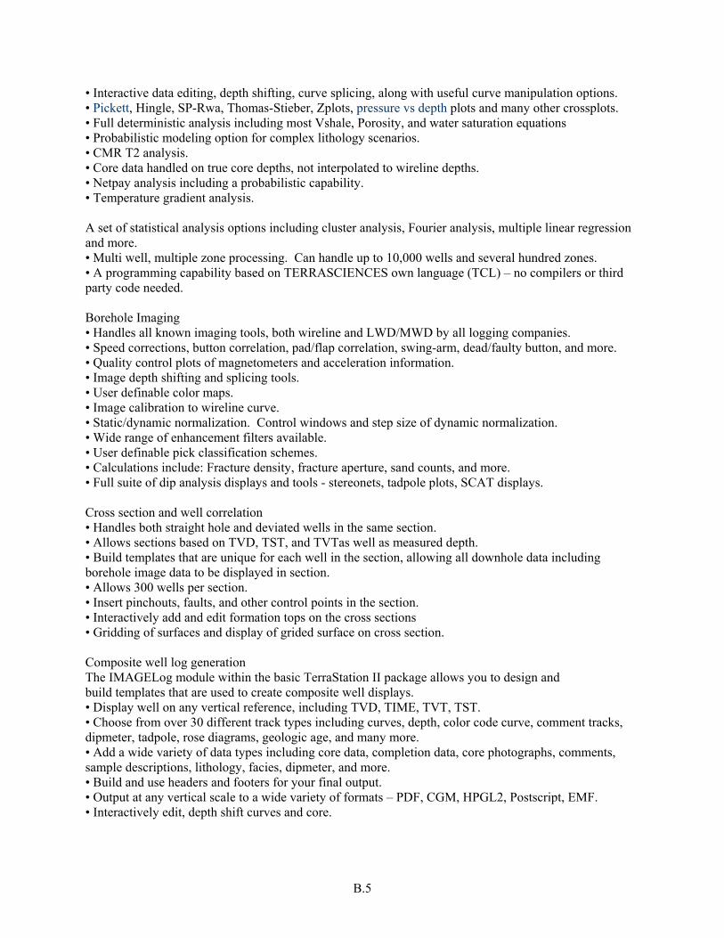
B.5

• Interactive data editing, depth shifting, curve splicing, along with useful curve manipulation options. • Pickett, Hingle, SP-Rwa, Thomas-Stieber, Zplots, pressure vs depth plots and many other crossplots. • Full deterministic analysis including most Vshale, Porosity, and water saturation equations • Probabilistic modeling option for complex lithology scenarios. • CMR T2 analysis. • Core data handled on true core depths, not interpolated to wireline depths. • Netpay analysis including a probabilistic capability. • Temperature gradient analysis. A set of statistical analysis options including cluster analysis, Fourier analysis, multiple linear regression and more. • Multi well, multiple zone processing. Can handle up to 10,000 wells and several hundred zones. • A programming capability based on TERRASCIENCES own language (TCL) – no compilers or third party code needed. Borehole Imaging • Handles all known imaging tools, both wireline and LWD/MWD by all logging companies. • Speed corrections, button correlation, pad/flap correlation, swing-arm, dead/faulty button, and more. • Quality control plots of magnetometers and acceleration information. • Image depth shifting and splicing tools. • User definable color maps. • Image calibration to wireline curve. • Static/dynamic normalization. Control windows and step size of dynamic normalization. • Wide range of enhancement filters available. • User definable pick classification schemes. • Calculations include: Fracture density, fracture aperture, sand counts, and more. • Full suite of dip analysis displays and tools - stereonets, tadpole plots, SCAT displays. Cross section and well correlation • Handles both straight hole and deviated wells in the same section. • Allows sections based on TVD, TST, and TVTas well as measured depth. • Build templates that are unique for each well in the section, allowing all downhole data including borehole image data to be displayed in section. • Allows 300 wells per section. • Insert pinchouts, faults, and other control points in the section. • Interactively add and edit formation tops on the cross sections • Gridding of surfaces and display of grided surface on cross section. Composite well log generation The IMAGELog module within the basic TerraStation II package allows you to design and build templates that are used to create composite well displays. • Display well on any vertical reference, including TVD, TIME, TVT, TST. • Choose from over 30 different track types including curves, depth, color code curve, comment tracks, dipmeter, tadpole, rose diagrams, geologic age, and many more. • Add a wide variety of data types including core data, completion data, core photographs, comments, sample descriptions, lithology, facies, dipmeter, and more. • Build and use headers and footers for your final output. • Output at any vertical scale to a wide variety of formats – PDF, CGM, HPGL2, Postscript, EMF. • Interactively edit, depth shift curves and core.

B.6

Mapping • Contour maps with a variety of display options. • Perspective block diagrams of up to 4 computed surfaces. • Gridding, triangulation and kriging capability. • Posting of well displays on map at well locations. • Pie charts, starburst maps and other posting capabilities. • Compute mappable values from log data using a variety of computation options. • Surface to surface computation capabilities on both raw data and computed grids. • Import and export of grids. Organic Geochemistry from Wireline Data A specialized module for those looking into source rock distribution and analysis. The module provides a way to obtain many of the same outputs that a RockEval laboratory analysis would provide. Advantages include: • A more comprehensive coverage in the well – same as the wireline logs used. • Provides values where no cuttings or other samples are available. • Avoids problem of ‘bit metamorphism’ caused by high bit rotation speeds destroying potential samples. • Geochemistry specific crossplots and overlays – TOC vs S2, Van Krevelen, modified van Krevelen. Sonic Waveform Processing A module for analyzing and processing full waveform sonic logs is available. It includes: • Handles both monopole and dipole tools. • Filters for noise removal, including bandpass filter. • Semblance contouring function. • Compute compressional, shear, and Stonely arrivals. • Display instantaneous phase, amplitude, and frequency. • Frequency dispersion correction available.

Interactive Petrophysics (http://www.slb.com/content/services/software/geo/intpetro/index.asp; last accessed September 30, 2009) Interactive Petrophysics™ was developed by Senergy (http://www.senergyltd.com) and is exclusively sold and marketed by Schlumberger. It performs various tasks associated primarily with analyzing wireline log data, including:

• Log Plotting and Cross Plotting • Resistivity Temperature Corrections • Downhole Water Density Calculations • Porosity/Water Saturation Calculations • Pore Pressure Prediction • NML or NMR Log Interpretation • Clay Volume Estimation • Elastic Impedance Calculation • Capillary Pressure Function Calculation • Fuzzy Logic Estimation of Missing Log Intervals • Monte Carlo Error Analysis • Neural Network Prediction • Mineral Solver

o Compositional analysis using singular value decomposition • Cluster Analysis

B.7

• Principal Component Analysis The license fee for the base Interactive Petrophysics module is $15,000. As with Petrel, additional functionality is provided through add-on modules that cost extra, but it is not clear how many of the features listed above actually come with the base module. The Mineral Solver is an add-on module that costs $8,800 so the base module plus the Mineral Solver would cost a total of $23,800 (personal communication with Mike Mroz, PNNL Account Manager for Schlumberger Information Solutions, August 5, 2009). As with other Schlumberger software products, the annual maintenance fee is 20% of the total cost of all supported modules. So for Interactive Petrophysics plus the Mineral Solver the annual maintenance fee would be $4,760. PNNL does not currently own a license for the Interactive Petrophysics software. PfEFFER Pro (http://www.kgs.ku.edu/PRS/software/pfeffer2.html; last accessed September 30, 2009) and KIPLING (http://www.kgs.ku.edu/software/Kipling/; last accessed September 30, 2009) Pfeiffer and Kipling are two separate software packages, implemented as Excel™ add-ins, that were developed by Geoffrey Bohling and John Doveton of the Kansas Geological Survey (KGS) in Lawrence, Kansas. Combined, these two packages perform many (but not all) of the functions that are available in the Interactive Petrophysics software marketed by Schlumberger, and other similar packages, but for a fraction of the cost. Modules in PfEFFER Pro include:

• Reading LAS digital files • Hough transform for simultaneous solution of Archie equation constants and formation water

resistivity • Log display • Calculation of porosity with option for shale correction and secondary porosity • Constructing a "Super Pickett" crossplot annotated with lines of water saturation, bulk volume

water, and permeability • Shaly sand models for Sw calculation • Moveable oil plots and calculations • Pay-flag cutoffs • Lithology solution • Capillary-pressure analysis • Zonation by depth • “First look” (simple) Mapping • Color-image cross section generation • Latitude-longitude to UTM conversion • Bridging software to build input file for a reservoir simulator • Zonation by depth-constrained hierarchical cluster analysis (Ward’s method)

PfEFFER Pro costs $350 plus $7 shipping Kipling is an Excel Add-in for Nonparametric Regression and Classification. The code can be used for either nonparametric regression or nonparametric descriminant function analysis to generate models for prediction of either continuous variables (such as permeability) or categorical variables (such as facies) from a set of predictor variables (eg. well log data). Kipling also contains code to compute a transition probability matrix from an observed sequence of categorical variables. Version 1 of Kipling costs $45

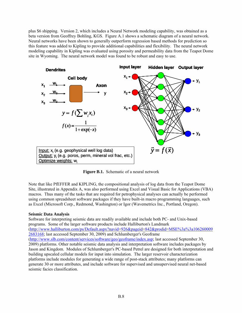
B.8

plus $6 shipping. Version 2, which includes a Neural Network modeling capability, was obtained as a beta version from Geoffrey Bohling, KGS. Figure A.1 shows a schematic diagram of a neural network. Neural networks have been shown to generally outperform regression based methods for prediction so this feature was added to Kipling to provide additional capabilities and flexibility. The neural network modeling capability in Kipling was evaluated using porosity and permeability data from the Teapot Dome site in Wyoming. The neural network model was found to be robust and easy to use.

Input: xi (e.g. geophysical well log data)Output: yi (e.g. poros, perm, mineral vol frac, etc.)Optimize weights: wi

x1

x2

x3

y1

y2

y3

)(xfy rr=

Input layer Hidden layer Output layer

y

)( iixwfy ∑=

w2

w1

w3

)exp(11)(

xxf

−+=

x1

x2

x3

Dendrites

Cell bodyAxon

Input: xi (e.g. geophysical well log data)Output: yi (e.g. poros, perm, mineral vol frac, etc.)Optimize weights: wi

x1

x2

x3

y1

y2

y3

)(xfy rr=

Input layer Hidden layer Output layer

y

)( iixwfy ∑=

w2

w1

w3

)exp(11)(

xxf

−+=

x1

x2

x3

Dendrites

Cell bodyAxon

x1

x2

x3

y1

y2

y3

)(xfy rr=

Input layer Hidden layer Output layer

x1

x2

x3

y1

y2

y3

)(xfy rr=

Input layer Hidden layer Output layer

y

)( iixwfy ∑=

w2

w1

w3

)exp(11)(

xxf

−+=

x1

x2

x3

Dendrites

Cell bodyAxon

y

)( iixwfy ∑=

w2

w1

w3

)exp(11)(

xxf

−+=

x1

x2

x3

Dendrites

Cell bodyAxon

Figure B.1. Schematic of a neural network

Note that like PfEFFER and KIPLING, the compositional analysis of log data from the Teapot Dome Site, illustrated in Appendix A, was also performed using Excel and Visual Basic for Applications (VBA) macros. Thus many of the tasks that are required for petrophysical analyses can actually be performed using common spreadsheet software packages if they have built-in macro programming languages, such as Excel (Microsoft Corp., Redmond, Washington) or Igor (Wavemetrics Inc., Portland, Oregon). Seismic Data Analysis Software for interpreting seismic data are readily available and include both PC- and Unix-based programs. Some of the larger software products include Halliburton's Landmark (http://www.halliburton.com/ps/Default.aspx?navid=926&pageid=842&prodid=MSE%3a%3a1062600092683168; last accessed September 30, 2009) and Schlumberger's Geoframe (http://www.slb.com/content/services/software/geo/geoframe/index.asp; last accessed September 30, 2009) platforms. Other notable seismic data analysis and interpretation software includes packages by Jason and Kingdom. Modules of Schlumberger's PC-based Petrel are designed for both interpretation and building upscaled cellular models for input into simulation. The larger reservoir characterization platforms include modules for generating a wide range of post-stack attributes; many platforms can generate 30 or more attributes, and include software for supervised and unsupervised neural net-based seismic facies classification.

B.9

GSLIB (http://www.gslib.com/; last accessed September 30, 2009) GSLIB is the standard for geostatistical analysis. Most commercial (e.g., Petrel) and open source geostatistical packages incorporate the GSLIB subroutines. Version 2 of the software is included on a CD published with the user’s manual (Deutsch and Journel 1998). All of the programs are available in Fortran source code and must be compiled by the user. No user interface is included, but the programs can be implemented through shell, Perl, or Python scripts to automate much of the data analysis. Capabilities in GSLIB include:

• Variogram calculation programs for scattered data and data on a regular grid o Both 2D and 3D data can be analyzed o Several measures of spatial continuity, including variogram, covariance, correlogram,

robust variograms, and cross covariance • Kriging

o Simple kriging o Ordinary kriging o Kriging with secondary data (e.g., kriging with a trend or an external drift) o Indicator kriging, including forms with secondary data (e.g., Markov-Bayes) o Co-kriging of multiple variables

• Simulation o Sequential Gaussian simulation

Secondary data can be incorporated using locally varying means, an external drift variable, or collocated cokriging

o Sequential indicator simulation Categorical data Continuous data Incorporation of secondary data

o Boolean simulation program (elliptical shapes only) o Simulated annealing

Allows incorporation of multiple objectives into simulation, e.g., matching one or more target variograms, a histogram, and/or correlation with a secondary variable

• Utilities o A large number of utilities are included for display, exploratory data analysis, data

transformations and back transforms, and postprocessing of indicator kriging and simulation results generated using any of the stochastic simulation algorithms

SGeMS (http://sgems.sourceforge.net/; last accessed Spetember 30, 2009) S-GeMS is public domain geostatistical software developed at Stanford for 3D geostatistical modeling. Many of the classical geostatistics algorithms implemented in GSLIB are included, as well as new developments from the geostatistics program at Stanford University. The most important of these is the inclusion of programs for multiple point geostatistics, a major advance beyond the two-point statistical methods available in GSLIB. Unlike GSLIB, SGeMS includes a graphical user interface (GUI) that makes it easier to use for those with limited programming experience. The availability of interactive variogram calculation and modeling in three dimensions is especially useful. SGeMS also includes strong links to the programming language Python, so scripts and automation are available to those with more extensive programming background. There is a reference book on SGeMS with datasets and the program included on a CD (Remy et al. 2009), but the most recent version of the software should be obtained from the link given above. Capabilities in SGeMS include:

• Variogram calculation programs for scattered data and data on a regular grid

B.10

o Both 2D and 3D data can be analyzed o Several measures of spatial continuity, including variogram, covariance, correlogram,

robust variograms, and cross covariance • Kriging

o Simple kriging o Ordinary kriging o Kriging with secondary data (e.g., kriging with a trend or an external drift) o Indicator kriging, including forms with secondary data (e.g., Markov-Bayes) o Co-kriging of multiple variables

• Simulation o Sequential Gaussian simulation

Secondary data can be incorporated using locally varying means, full cokriging, or two forms of the Markov assumption

o Sequential indicator simulation Categorical data Continuous data Incorporation of secondary data

o Block simulations to allow better integration of point and block data o Multiple point simulation

Includes two programs, snesim and filtersim, for stochastic simulation Snesim only works with categorical variables, while filtersim generates

simulations of both categorical and continuous variables. However, snesim is considered the more robust program of the two

The program includes an object-based simulator that can be used to produce the training images needed for multiple point simulation.

• Utilities o A large number of utilities are included for display, exploratory data analysis, data

transformations and back transforms, and postprocessing of indicator kriging and simulation results generated using any of the stochastic simulation algorithms

Roxar, Irap RMS Suite (http://www.roxar.com/iraprms/; last accessed September 30, 2009 ) Roxar’s Irap RMS Software Suite offers two Facies Modeling modules.RMSfacies offers a range of methods for the modeling of geological facies and lithology, including Roxar’s unique object modeling methods, as well as a truncated Gaussian method for transitional environments. Object modeling not only produces results that look geological, but unlike pixel based methods the objects explicitly preserve connectivity. This connectivity may be crucial in some reservoirs when predicting CO2 migration during injection. Roxar’s facies modeling tools are “the best available” at matching large numbers of wells as well as seismic attributes and trends. Directly observed seismic geobodies can also be correctly incorporated into the model using Roxar’s unique FaciesSedseis tool. Facies Modeling “features” include:

• Facies:Belts, an indicator-based modeling designed to model the stacking of facies belts in progradational, aggradational and retrogradational depositional systems, using geologically derived information such as dip, azimuth, and geometry.

• Facies:Composite, an object-modeling method that can used to describe a wide range of geological environments and facies geometries, using predefined and user editable objects, and azimuth trends to enable large facies objects to accurately follow detailed depositional trends.

• Facies:Channels, an object-modeling method specifically designed for describing channel reservoirs, including channels, channel margin facies (crevasses and levee) and intra-channel heterogeneities (gravel-lag thief zones, shale barriers).

B.11

• Facies:Sedseis, an object based modeling technique for allowing interpreted facies bodies (from high resolution seismic) to constrain the modeling of true 3D facies objects.

RMSindicators (Facies:Indicator) is an Indicator Facies Modeling module that includes Roxar’s own advanced sequential indicator simulation (SIS), a pixel based modeling method “ideal for large reservoirs or reservoirs with thousands of wells”. It includes a wide range of options for trend control of the model, including vertical proportion curves and seismic attributed data, and robust volume fraction control, to ensure accurate distribution of facies. The SIS algorithm is very flexible and also includes accurate volume matching constraints to ensure reliable results. The algorithm is extremely fast and flexibile making it ideal where there is a large amount of reservoir data available. The algorithm ensures accurate matching of the input volume fractions, including accurate honoring of vertical and horizontal facies proportions. Two options are available for conditioning to seismic data (conditional probabilities, and indicator co-simulation). Merged Facies Modeling. Roxar allows facies modeling results to be merged in any sequence, allowing for the modeling of hierarchial heterogeneities and more complex facies environments. The merged models can be comprised of any combination of indicator or object models. Geomodeling Technology (http://www.geomodeling.com/; Last accessed Septmber 30, 2009) Geomodeling Technology’s SBEDStudio is designed to integrate well log, seismic, stratigraphic, lithofacies and petrophysical data to build geologically realistic reservoir models. It includes a Facies Modeling component as part of its workflow, however, the details of the algorithms available are not defined. Geomodeling Technology also has a software product called SBED for small-scale (centimeter- to meter-scale) geological heterogeneity modeling and upscaling. BeicipFranblab’s Dionisos (http://www.beicip.com/index.php/eng/software/petroleum_systems_modeling/dionisos; last accessed September 30, 2009) Dionisos enables modeling of sedimentary processes for developing high resolution stratigraphic models. It is designed to quantitatively assess the complex interaction between accommodation space, sediment supply, and transport, through coupled simulation of sedimentary processes (fluvial, marine to coastal silico-clastic, carbonates). It produces physically sound geo-history of sedimentary basin development, featuring sedimentary architecture, lithologic facies and paleo-bathymetry evolution through space and time. Rock Solid Images LithANN (http://www.rocksolidimages.com/LithANN.htm; last accessed September 30, 2009) LithANN uses advanced neural network algorithms to define regions of common attribute response or seismic facies. It allows the user to combine two or more seismic attribute volumes to maximize the discriminatory capabilities of each attribute. LithANN offers several classification algorithms, including feed-forward back-propagating artificial neural networks and Kohonen Self Organizing Map (KSOM) methods. The output is a classified volume where each seismic sample is replaced by a class value representing the seismic facies.

B.12

Geovariances ISATIS (http://www.geovariances.com/; last accessed September 30, 2009) ISATIS provides easy access to all proven geostatistical techniques within a user-friendly interface. ISATIS’s Facies modeling capabilities include: Sequential Indicator Simulations (SIS), Truncated Gaussian Simulations (TGS), Plurigaussian Simulations (PGS), boolean simulations, Multiple-point Simulations. Plurigaussian simulation is designed to model complex geology with different structure orientations and heterogeneous deposits (e.g. channels, reefs, bars, differently oriented facies, sets of conjugate veins or ore types). Its ISATOIL module provides a 2D modeling technique for building a consistent 3D, stacked sequence (layered geological model) using an original global multi-layer approach.

PNNL-18844

Distribution

No. of Copies

Distr.1

# Local Distribution Pacific Northwest National Laboratory Diana Bacon (PDF) Gary Black (PDF) Alain Bonneville (PDF) Mike Fayer (PDF) Ian Gorton (PDF) George Last (PDF) Pete McGrail (PDF) Ellyn Murphy (PDF) Chris Murray (PDF) Karen Schuchardt (PDF) Charlotte Sullivan (PDF)

Paul Thorne (PDF) Mark White (PDF) Mark Williams (PDF) Signe Wurstner (PDF)