DRAINAGE RESEARCH IN FARMERS’ FIELDS: ANALYSIS OF DATA Part of project “Liquid Gold” of the International Institute for Land Reclamation and Improvement (ILRI), Wageningen, The Netherlands. R.J.Oosterbaan, July 2002 On website https://www.waterlog.info public domain, latest upload 20-11-2017 TABLE OF CONTENTS

1. Analysis of data.......................................................2 1.1 Types of analysis ..................................................2 1.2 Parameters .........................................................2

2. Standard statistical analysis..........................................4 2.1 Frequency analysis .................................................4 2.2 Time-series analysis ..............................................21 2.3 Testing of differences ............................................27 2.4 Spatial differences ...............................................29 2.5 Correlation analysis ..............................................30

3. Conceptual statistical analysis.......................................33 3.1 Linear regression, ratio method ...................................34 3.2 Linear regression, least squares method ...........................35 3.3 Intermediate regression ...........................................44 3.4 Segmented two-variable linear regression ..........................48 3.5 Segmented three-variable linear regression ........................56 3.6 Partial segmented linear regression ...............................60

4. Conceptual deterministic analysis.....................................61 4.1 Introduction ......................................................61 4.2 Transient recharge-discharge relations ............................63

References...............................................................70 Note: for additional information on section 3.4 see article on website: https://ww.waterlog.info/pdf/segmregr.pdf

2

1. Analysis of data

1.1 Types of analysis In drainage pilot areas one collects a large number of data that usually show a large variation (scatter). The analysis of the data aims at reaching conclusions, despite the scatter, on the drainage aspects of the pilot area proper, and recommendations for application to a wider area. The methods of analysis can be distinguished three types: - 1 standard statistical types; - 2 conceptual statistical types; - 3 conceptual deterministic types. The standard types are done routinely to assess the characteristics of the measured parameters and to detect trends. They are free of concepts about mutual influences between the measured parameters and the processes occurring between them. Despite this, they may yield important conclusions. The conceptual methods include assumptions about cause-effect relations between the measured parameters and aim at expanding the conclusions and recommendations found from the standard types. They require insight and originality of the researcher. With the conceptual statistical methods one derives the conclusions by relating the data to each other on the basis of certain hypotheses. These methods can also be called deductive or empirical methods. With the conceptual deterministic, or inductive, methods one applies deterministic theories, concepts and models, which describe the expected relations between their parameters, using some of the measured data as input and checking the outcomes with other measured data. In the process one can try to adjust parts of the theory to obtain a better match of measured and calculated results, using a match index. This process is called calibration and is done by trial and error.

1.2 Parameters The number of method types within each group is high. They are discussed in the next sections assuming that at least the following parameters have been measured: 1 - Crop yields 2 - Depth of the water table 3 - Soil salinity, alkalinity, and acidity 4 - Hydraulic conductivity 5 - Drain discharge 6 - Rainfall 7 - Irrigation

3

The examples given in the following text refer to the above parameters. The last three parameters are double time dependent. The implications of this are discussed later. In drainage research many more than the above 7 parameters may have been measured. The principles and examples that will be given further on can also be applied to these.

4

2. Standard statistical analysis It is recommended that the standard methods of statistical analysis be applied routinely to all parameters that have been measured repeatedly with the aim to present the mass of data in a surveyable manner rather than in the form of long lists and tables. Further the analysis serves the purpose of reaching preliminary conclusions or detecting unexpected features. The standard methods can be applied to the entire mass of measured values of the parameter, or on their subdivision into groups representing different periods of time, sub-areas or treatments. The standard methods mainly comprise the statistical analysis of: 1 - Frequencies; 2 - Time-series; 3 - Correlations. Frequency analysis is used to assess the order magnitude of measured parameters and factors, evaluate their variability, and to judge how often a certain range of values occurs. Time series are made of time dependent data to obtain insight in the time-variation and/or time-trends. Correlation analysis is applied to detect a trend between two or more parameters/factors (henceforth called variables) even though the relation between them is diffuse (scattered). The detection of time-trends can also be done by correlation. Variables do not only change in time but also in space. The spatial

variation is more complicated than the time variation in the sense that more than one dimension is involved. No simple standard statistical technique is available for the spatial analysis of a variable. Yates and Warrick (1999) advocate the use of the more complex technique of Kriging. A relatively simple way to analyse spatial differences and trends is by dividing the study area into sub-areas, applying the above statistical techniques separately for each sub-area, and comparing the results. The subdivision of the area needs sound judgement. The above analysis methods will be subsequently discussed.

2.1 Frequency analysis To obtain insight in the scatter or variation of measured values of a parameter, it has long been common practice to calculate of each measured variable the mean (µ) and the standard deviation (σ). The mean gives an estimate of the central point of the mass of data and the standard deviation gives an estimate of the closeness of the data to the mean. Nowadays, with spreadsheet computer programs, it is fairly easy to straightaway determine frequency distributions of the parameters along with µ, σ, mode, and median. Therefore, it is recommended to routinely apply the more informative frequency analysis than the simpler common practice used hitherto. The frequency analysis can also be a tool of data screening.

5

The computer program CumFreq (see www.waterlog.info/cumfreq.htm ) automates the calculation of cumulative frequency distributions. It uses a fairly large number of different mathematical expressions of frequency distributions and selects the expressions that give the best match with the data. In addition, it provides interval analysis, confidence belts, and graphics. One can start the frequency analysis using the ranking method. When the data are ranked in ascending order, the value F = 100 R/(n+1) where R is the rank number and n the number of data, indicates the cumulative frequency (%), i.e. the frequency of non-exceedance (%), or the percentage of data with values smaller than the value considered. The value 1-F indicates the frequency of exceedance. When the data and their frequencies are plotted on linear graphic paper one will see that despite the existence of scatter, the data tend to form a curved line. The curved line indicates the type of frequency distribution and the scatter is assumed to stem from random variation. Though not strictly required, one often tries to eliminate the curvature by plotting the data on probability paper. There are different papers for different types of distribution. If the curvature cannot be fully eliminated by this method, one can try to use transformed data (e.g. their log values). An example of this linearization will be given later. To illustrate the application of frequency analysis, the following examples will be given: - Means and standard deviations - Cumulative frequencies of crop yield. - Cumulative frequencies of water-table depth; - Cumulative frequencies of soil salinity; - Cumulative and interval frequencies of hydraulic conductivity; - Cumulative frequencies of rainfall; - Cumulative frequencies of river discharge; - Cumulative frequencies of drain discharge. Having gone through the examples, a brief discussion follows on "missing data" and the presence of "outliers".

Means and standard deviations To obtain insight in the scatter or variation of measured values of a parameter, it has long been common practice to calculate of each measured variable the mean (µ) and the standard deviation (σ). The mean gives an estimate of the central point of the mass of data and the standard deviation gives an estimate of the closeness of the data to the mean. A table with means and standard deviations of variables can provide essential information at a quick glance.

6

Table 1. Chemical parameters of the ground water in the experimental fields of Tatas by water-management trial. ───────────────────────────────────────────────────────────────── Irrigation treatment *) Chem. ------------------------------------------------------- para- with canal water with swamp water no irrigation meter ---------------- ---------------- ------------- mean st.dev. mean st.dev. mean st.dev. ----------------------------------------------------------------- pHH2O 3.8 0.43 3.7 0.37 3.7 0.37 SO4-- 3.4 1.9 4.3 1.9 3.7 1.9 Fe++ 0.85 0.54 1.1 0.68 0.90 0.64 Mg++ 0.82 0.50 0.98 0.52 0.88 0.54 Al+++ 0.86 0.64 1.1 0.63 0.96 0.71 ───────────────────────────────────────────────────────────────── *) The number of data per treatment varies between 576 and 597 Ion concentrations are in me/l As an illustration, table 1 shows the means (µ) and standard deviations (σ) of some chemical soil data by water-management trial (Oosterbaan 1990). It concerns different irrigation treatments in the Tatas pilot area near Bandjermasin, Kalimantan, Indonesia. The pilot area is situated in acid sulphate soils on the island of Pulau Petak. The data are discussed below. The pH Values It can be seen that the pH (acidity) values have relatively small standard deviations (about 10% of the mean). This indicates that the values are closely grouped around the mean and that they are fairly constant. Hence, the pH is a dependable characteristic of the soil. Assuming that the data are normally distributed, the interval around the mean in which some 95% of the pH data is found, i.e. the 95% occurrence

interval, can be roughly determined from an upper confidence limit U and a lower confidence limit V as follows: U = µ + 2σ V = µ - 2σ In theory, the factor 2 is to be replaced by Student's statistic t. This is discussed in section 1.4. Using the above relations, and rounding off the standard devotions to the value σ = 0.4, it can be found from table 1 that the 95% occurrence interval of all the pH data ranges approximately between 2.9 and 4.6. The mean values of the pH for the different treatments are almost the same (3.8, 3.7, and 3.7). The variation between the means is much smaller than the already fairly small standard deviations. Without further statistical

7

tests, it can be concluded that the different treatments have hardly any influence on pH. The sulphates The values of the SO4= (sulphate) concentration, on the other hand, have higher standard deviations, in the order of 50% of the means (ranging from 44 to 55%). It is not possible to determine the 95% occurrence interval with the method discussed before, as one would obtain negative values. The used assumption of normally distributed values is not valid. Apparently, the distribution is a-symmetrical (skew) and one would need to investigate the complete frequency distribution to assess the occurrence intervals. The variation between the means is also larger than in the pH example. Therefore, contrary to the pH example, the standard statistical analysis using means and standard deviations of SO4= gives no straightforward conclusion about the influence of the treatment. To judge if the mean SO4= value in the swamp-water treatment (µ = 4.3 me/l) and the canal-water treatment (µ = 3.4 me/l) is statistically significant, and not due to random variation, one can estimate the upper limit µu and lower limit µv of the 95% confidence interval of µ from: µu = µ + 2σ/√n µv = µ - 2σ/√n where n is the number of data. Thus we find from table 1 with 95% confidence that the mean SO4= value in the canal-water treatment can vary between 3.2 and 3.6, and in the swamp-water treatment between 4.1 and 4.5. The method of means and standard deviations shows that the first irrigation treatment is definitely related to lower sulphate contents than the second. It remains to be seen if this is the result of the treatment itself or if some other circumstances also play a role. In theory, the differences between the treatments must be tested using the t statistic and the standard deviation of the difference between the µ values. This is discussed in section 2.3. In this example, however, the theoretical test would not lead to a different conclusion. The metals The standard deviations of the concentrations of the metals Fe++ (iron), Mg++ (magnesium) and Al+++ (aluminium) are, like those of the sulphates, quite high and more than 50% of the mean values. Owing to the large number of observations (almost 600), the test on the differences between the mean values of the concentrations of the metals in the different treatments would lead to the conclusion that they are indeed statistically significant. However, given the relatively large standard deviations (more than 50%), the differences between the means of the different treatments (in the order of 10 to 20%), even though statistically significant, are less interesting. In agricultural lands, differences between means of certain variables are

8

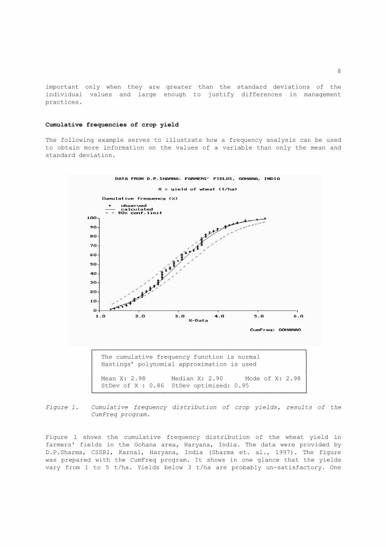
important only when they are greater than the standard deviations of the individual values and large enough to justify differences in management practices. Cumulative frequencies of crop yield The following example serves to illustrate how a frequency analysis can be used to obtain more information on the values of a variable than only the mean and standard deviation.

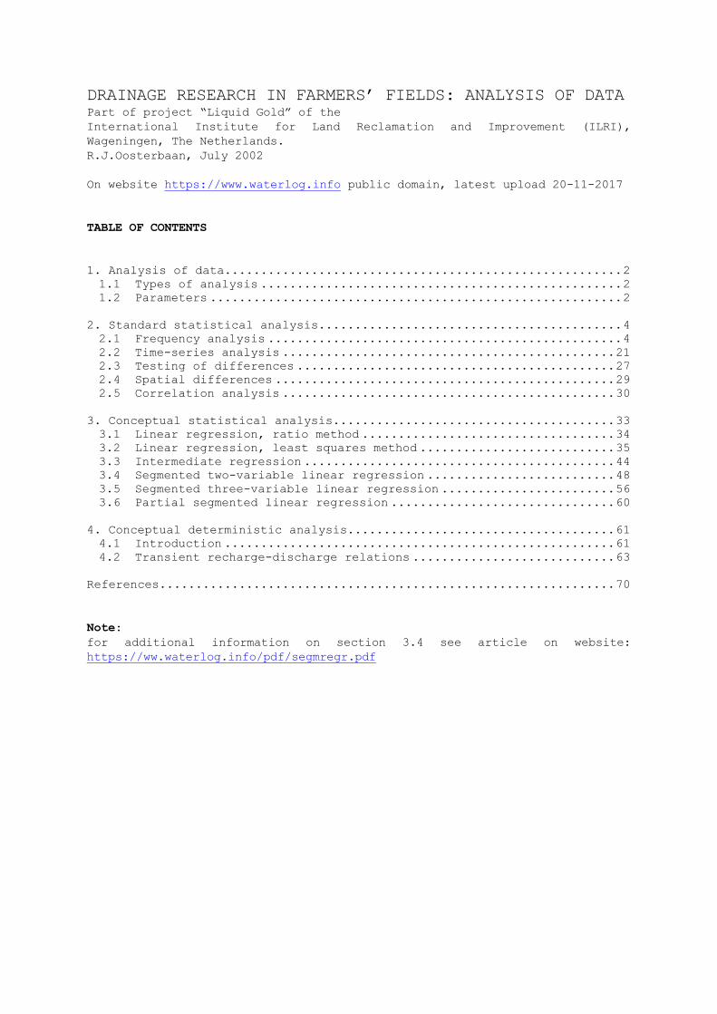
┌─────────────────────────────────────────────────────────┐ │ The cumulative frequency function is normal │ │ Hastings’ polynomial approximation is used │ │ │ │ Mean X: 2.98 Median X: 2.90 Mode of X: 2.98 │ │ StDev of X : 0.86 StDev optimised: 0.95 │ └─────────────────────────────────────────────────────────┘ Figure 1. Cumulative frequency distribution of crop yields, results of the

CumFreq program.

Figure 1 shows the cumulative frequency distribution of the wheat yield in farmers' fields in the Gohana area, Haryana, India. The data were provided by D.P.Sharma, CSSRI, Karnal, Haryana, India (Sharma et. al., 1997). The figure was prepared with the CumFreq program. It shows in one glance that the yields vary from 1 to 5 t/ha. Yields below 3 t/ha are probably un-satisfactory. One

9

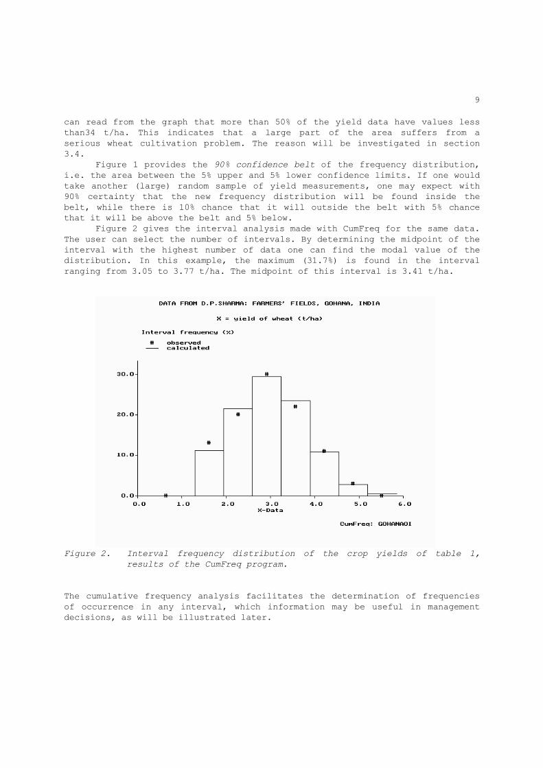
can read from the graph that more than 50% of the yield data have values less than34 t/ha. This indicates that a large part of the area suffers from a serious wheat cultivation problem. The reason will be investigated in section 3.4. Figure 1 provides the 90% confidence belt of the frequency distribution, i.e. the area between the 5% upper and 5% lower confidence limits. If one would take another (large) random sample of yield measurements, one may expect with 90% certainty that the new frequency distribution will be found inside the belt, while there is 10% chance that it will outside the belt with 5% chance that it will be above the belt and 5% below. Figure 2 gives the interval analysis made with CumFreq for the same data. The user can select the number of intervals. By determining the midpoint of the interval with the highest number of data one can find the modal value of the distribution. In this example, the maximum (31.7%) is found in the interval ranging from 3.05 to 3.77 t/ha. The midpoint of this interval is 3.41 t/ha.

Figure 2. Interval frequency distribution of the crop yields of table 1,

results of the CumFreq program.

The cumulative frequency analysis facilitates the determination of frequencies of occurrence in any interval, which information may be useful in management decisions, as will be illustrated later.

10

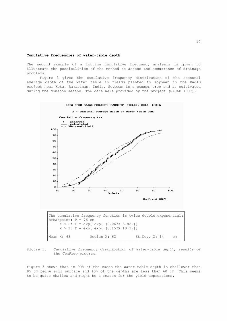
Cumulative frequencies of water-table depth The second example of a routine cumulative frequency analysis is given to illustrate the possibilities of the method to assess the occurrence of drainage problems. Figure 3 gives the cumulative frequency distribution of the seasonal average depth of the water table in fields planted to soybean in the RAJAD project near Kota, Rajasthan, India. Soybean is a summer crop and is cultivated during the monsoon season. The data were provided by the project (RAJAD 1997).

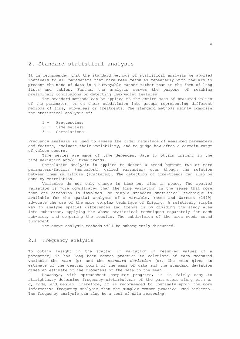
┌──────────────────────────────────────────────────────────────┐ │The cumulative frequency function is twice double exponential:│ │Breakpoint: P = 76 cm │ │ X < P: F = exp[-exp{-(0.067X-3.82)}] │ │ X > P: F = exp[-exp{-(0.153X-10.3)}] │ │ │ │Mean X: 63 Median X: 62 St.Dev. X: 14 cm │ └──────────────────────────────────────────────────────────────┘ Figure 3. Cumulative frequency distribution of water-table depth, results of

the CumFreq program.

Figure 3 shows that in 90% of the cases the water table depth is shallower than 85 cm below soil surface and 40% of the depths are less than 60 cm. This seems to be quite shallow and might be a reason for the yield depressions.

11

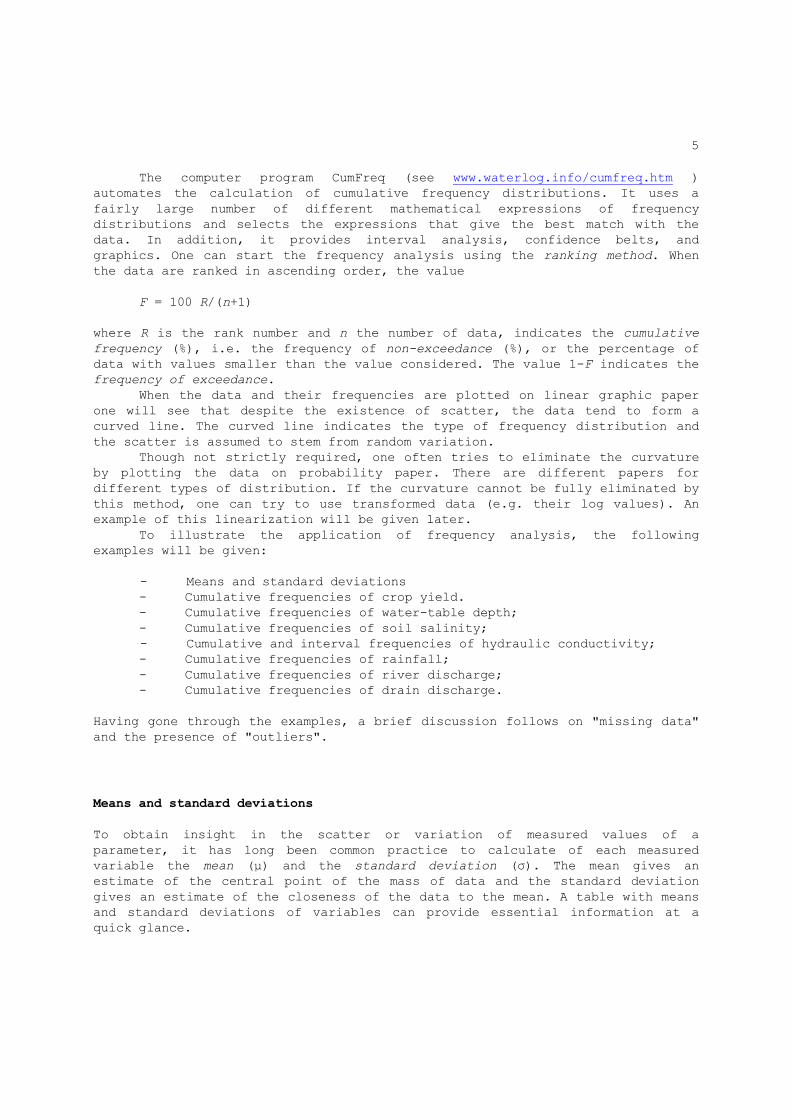
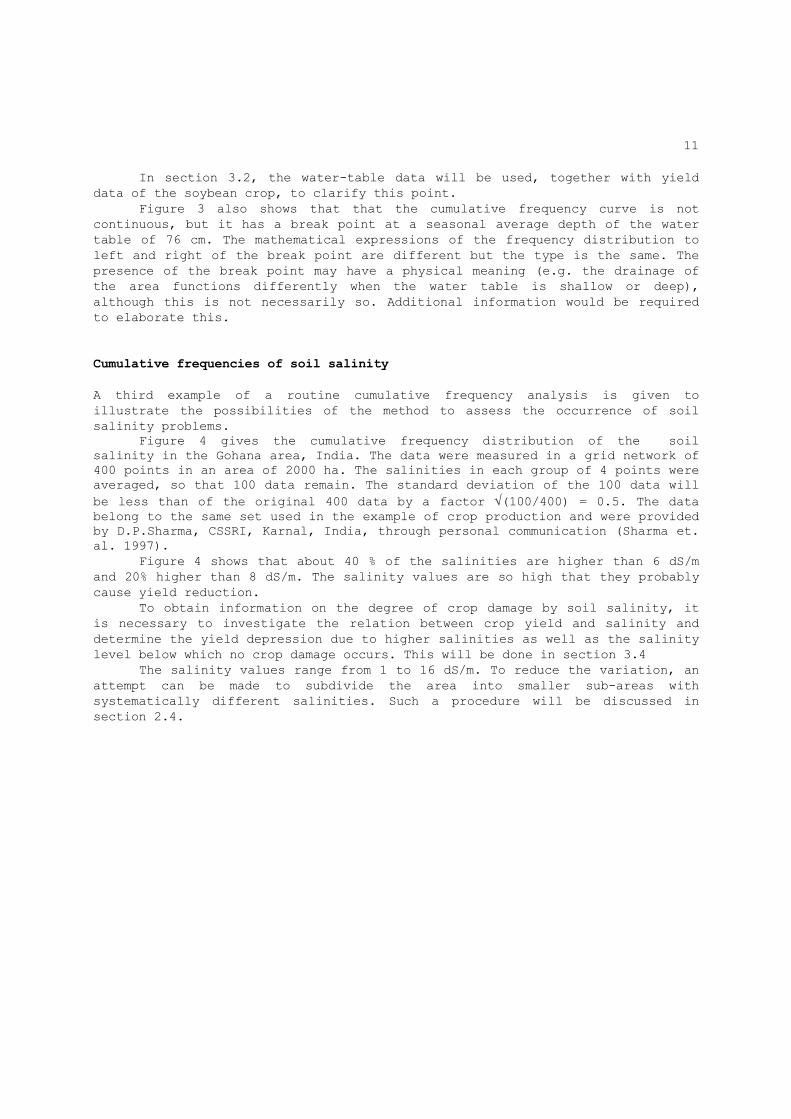
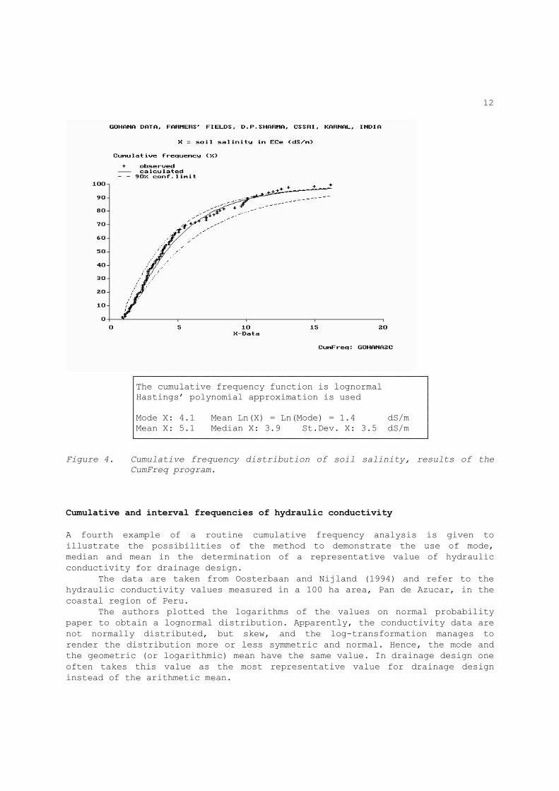
In section 3.2, the water-table data will be used, together with yield data of the soybean crop, to clarify this point. Figure 3 also shows that that the cumulative frequency curve is not continuous, but it has a break point at a seasonal average depth of the water table of 76 cm. The mathematical expressions of the frequency distribution to left and right of the break point are different but the type is the same. The presence of the break point may have a physical meaning (e.g. the drainage of the area functions differently when the water table is shallow or deep), although this is not necessarily so. Additional information would be required to elaborate this. Cumulative frequencies of soil salinity A third example of a routine cumulative frequency analysis is given to illustrate the possibilities of the method to assess the occurrence of soil salinity problems. Figure 4 gives the cumulative frequency distribution of the soil salinity in the Gohana area, India. The data were measured in a grid network of 400 points in an area of 2000 ha. The salinities in each group of 4 points were averaged, so that 100 data remain. The standard deviation of the 100 data will be less than of the original 400 data by a factor √(100/400) = 0.5. The data belong to the same set used in the example of crop production and were provided by D.P.Sharma, CSSRI, Karnal, India, through personal communication (Sharma et. al. 1997). Figure 4 shows that about 40 % of the salinities are higher than 6 dS/m and 20% higher than 8 dS/m. The salinity values are so high that they probably cause yield reduction. To obtain information on the degree of crop damage by soil salinity, it is necessary to investigate the relation between crop yield and salinity and determine the yield depression due to higher salinities as well as the salinity level below which no crop damage occurs. This will be done in section 3.4 The salinity values range from 1 to 16 dS/m. To reduce the variation, an attempt can be made to subdivide the area into smaller sub-areas with systematically different salinities. Such a procedure will be discussed in section 2.4.

12

┌──────────────────────────────────────────────────────┐ │The cumulative frequency function is lognormal │ │Hastings’ polynomial approximation is used │ │ │ │Mode X: 4.1 Mean Ln(X) = Ln(Mode) = 1.4 dS/m │ │Mean X: 5.1 Median X: 3.9 St.Dev. X: 3.5 dS/m │ └──────────────────────────────────────────────────────┘ Figure 4. Cumulative frequency distribution of soil salinity, results of the

CumFreq program.

Cumulative and interval frequencies of hydraulic conductivity A fourth example of a routine cumulative frequency analysis is given to illustrate the possibilities of the method to demonstrate the use of mode, median and mean in the determination of a representative value of hydraulic conductivity for drainage design. The data are taken from Oosterbaan and Nijland (1994) and refer to the hydraulic conductivity values measured in a 100 ha area, Pan de Azucar, in the coastal region of Peru. The authors plotted the logarithms of the values on normal probability paper to obtain a lognormal distribution. Apparently, the conductivity data are not normally distributed, but skew, and the log-transformation manages to render the distribution more or less symmetric and normal. Hence, the mode and the geometric (or logarithmic) mean have the same value. In drainage design one often takes this value as the most representative value for drainage design instead of the arithmetic mean.

13

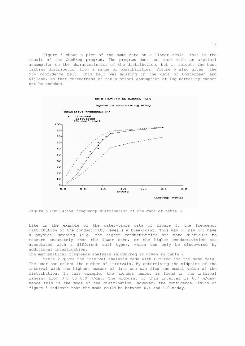
Figure 5 shows a plot of the same data on a linear scale. This is the result of the CumFreq program. The program does not work with an a-priori assumption on the characteristics of the distribution, but it selects the best fitting distribution from a range of possibilities. Figure 5 also gives the 95% confidence belt. This belt was missing in the data of Oosterbaan and Nijland, so that correctness of the a-priori assumption of log-normality cannot not be checked.

Figure 5 Cumulative frequency distribution of the data of table 2.

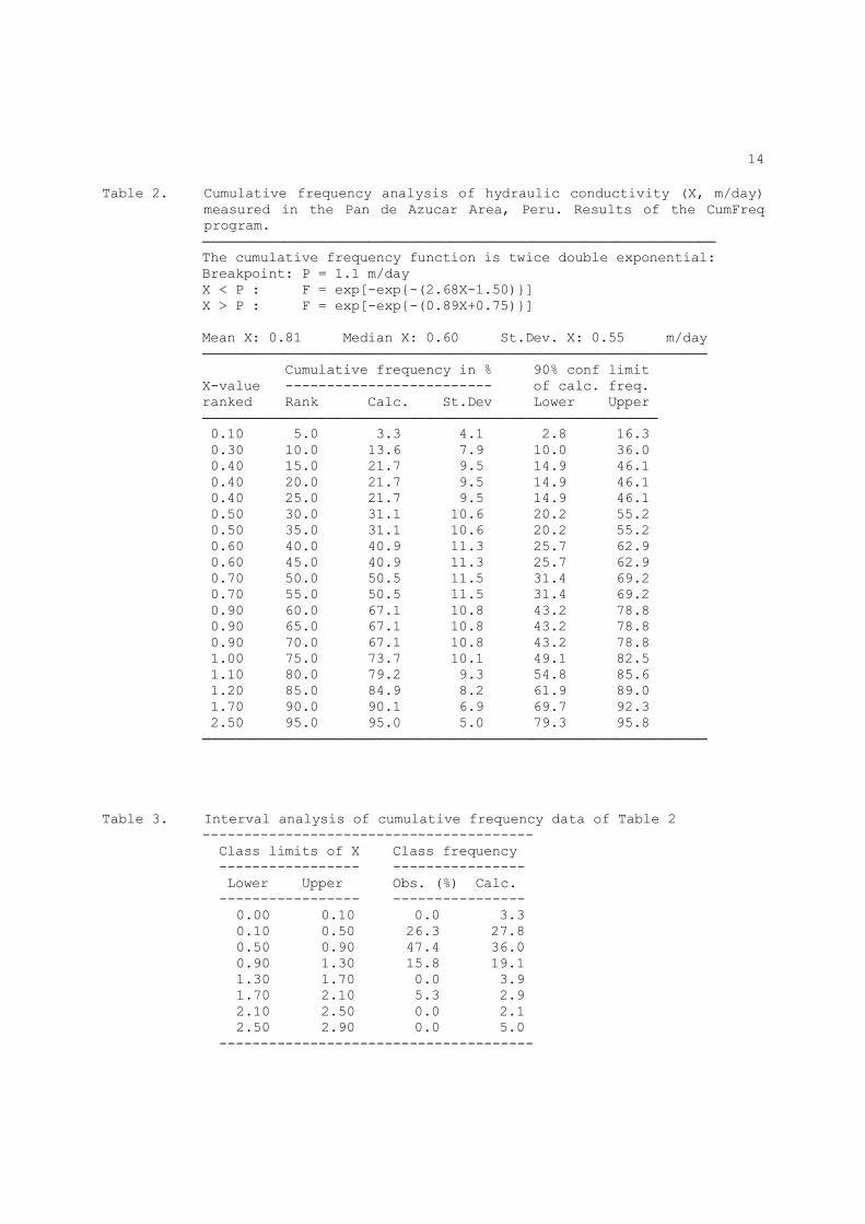
Like in the example of the water-table data of figure 3, the frequency distribution of the conductivity reveals a breakpoint. This may or may not have a physical meaning (e.g. the higher conductivities are more difficult to measure accurately than the lower ones, or the higher conductivities are associated with a different soil type), which can only be discovered by additional investigation. The mathematical frequency analysis in CumFreq is given in table 2. Table 2 gives the interval analysis made with CumFreq for the same data. The user can select the number of intervals. By determining the midpoint of the interval with the highest number of data one can find the modal value of the distribution. In this example, the highest number is found in the interval ranging from 0.5 to 0.9 m/day. The midpoint of this interval is 0.7 m/day, hence this is the mode of the distribution. However, the confidence limits of figure 5 indicate that the mode could be between 0.4 and 1.0 m/day.

14

Table 2. Cumulative frequency analysis of hydraulic conductivity (X, m/day) measured in the Pan de Azucar Area, Peru. Results of the CumFreq program.

────────────────────────────────────────────────────────────── The cumulative frequency function is twice double exponential: Breakpoint: P = 1.1 m/day X < P : F = exp[-exp{-(2.68X-1.50)}] X > P : F = exp[-exp{-(0.89X+0.75)}] Mean X: 0.81 Median X: 0.60 St.Dev. X: 0.55 m/day ───────────────────────────────────────────────────────────── Cumulative frequency in % 90% conf limit X-value ------------------------- of calc. freq. ranked Rank Calc. St.Dev Lower Upper ─────────────────────────────────────────────────────── 0.10 5.0 3.3 4.1 2.8 16.3 0.30 10.0 13.6 7.9 10.0 36.0 0.40 15.0 21.7 9.5 14.9 46.1 0.40 20.0 21.7 9.5 14.9 46.1 0.40 25.0 21.7 9.5 14.9 46.1 0.50 30.0 31.1 10.6 20.2 55.2 0.50 35.0 31.1 10.6 20.2 55.2 0.60 40.0 40.9 11.3 25.7 62.9 0.60 45.0 40.9 11.3 25.7 62.9 0.70 50.0 50.5 11.5 31.4 69.2 0.70 55.0 50.5 11.5 31.4 69.2 0.90 60.0 67.1 10.8 43.2 78.8 0.90 65.0 67.1 10.8 43.2 78.8 0.90 70.0 67.1 10.8 43.2 78.8 1.00 75.0 73.7 10.1 49.1 82.5 1.10 80.0 79.2 9.3 54.8 85.6 1.20 85.0 84.9 8.2 61.9 89.0 1.70 90.0 90.1 6.9 69.7 92.3 2.50 95.0 95.0 5.0 79.3 95.8 ───────────────────────────────────────────────────────────── Table 3. Interval analysis of cumulative frequency data of Table 2 ---------------------------------------- Class limits of X Class frequency ----------------- ---------------- Lower Upper Obs. (%) Calc. ----------------- ----------------

0.00 0.10 0.0 3.3 0.10 0.50 26.3 27.8 0.50 0.90 47.4 36.0 0.90 1.30 15.8 19.1 1.30 1.70 0.0 3.9 1.70 2.10 5.3 2.9 2.10 2.50 0.0 2.1 2.50 2.90 0.0 5.0

--------------------------------------

15

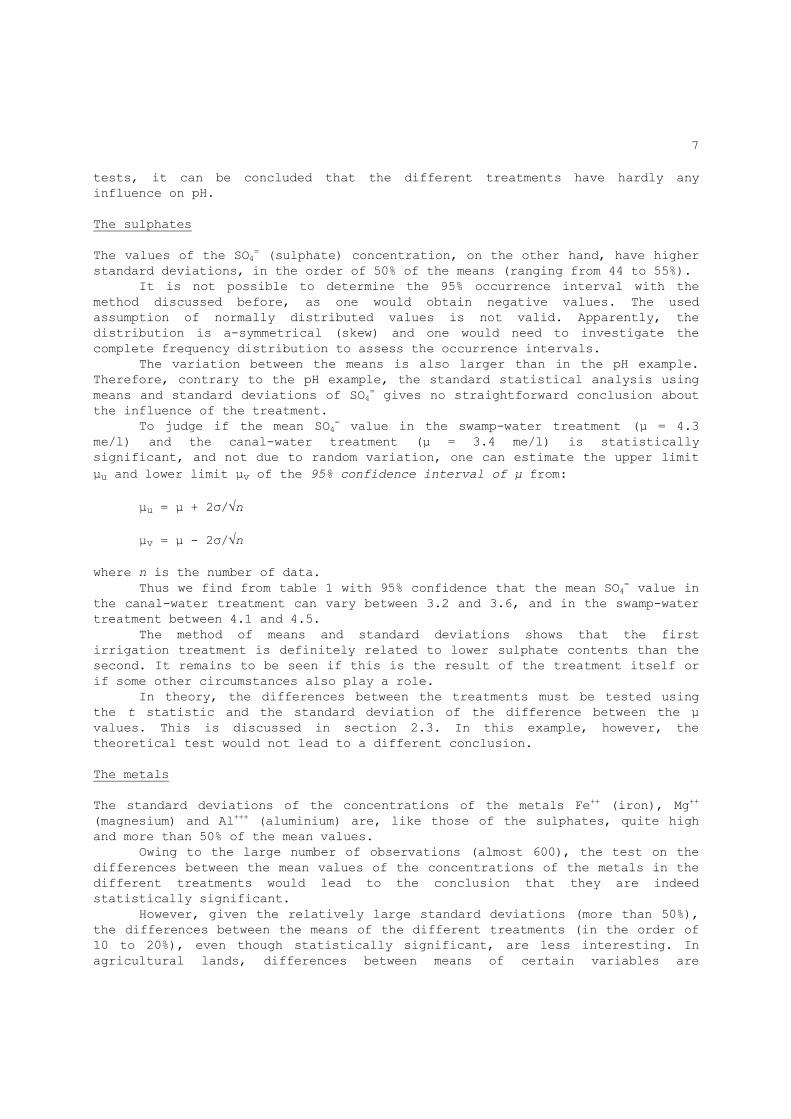
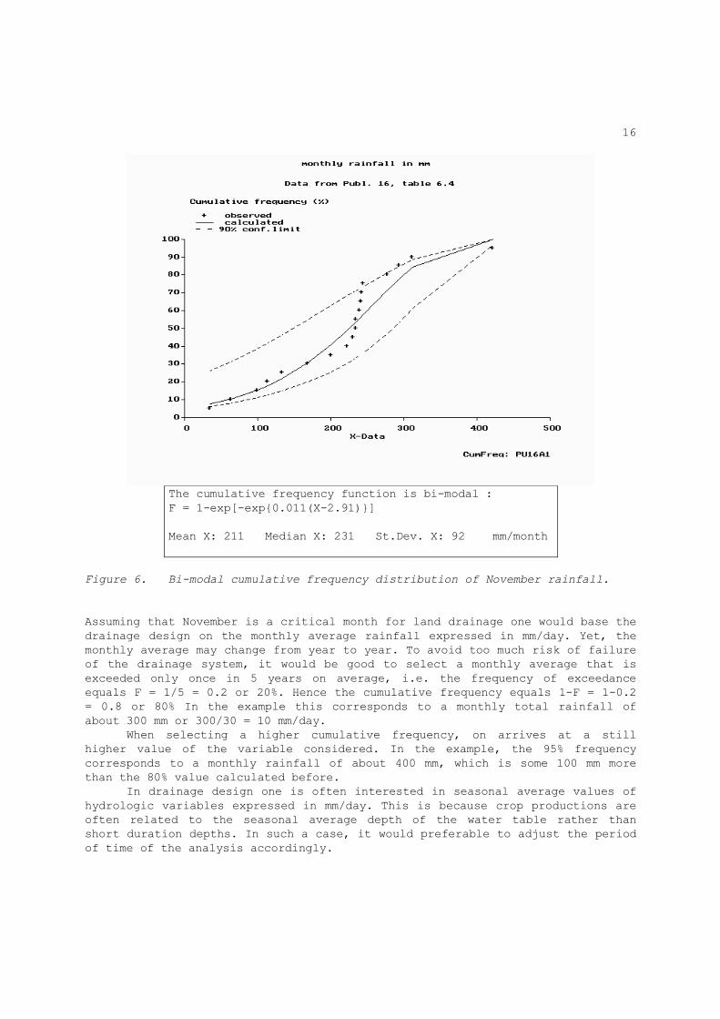
Accepting the lower of the last two values would result in a design that will seldom fail. However, the design would lead to a more costly system than when a higher conductivity value is taken. A benefit-cost analysis is required to find the optimal conductivity value for use in the design. Alternatively, the number of observations could be increased to obtain a narrower confidence belt. This illustrates the need for a quick frequency analysis of as soon as the data have been collected, so that a timely adjustment of the research program. The conductivity values range from 0.1 to 2.5 m/day. Soil scientists have reported that the area suffered from sodicity problems that would have a detrimental effect on soil structure and hydraulic conductivity. Fortunately, the data set used does not indicate a particularly poor hydraulic conductivity, so that the sodicity problems are limited. To reduce the variation, an attempt can be made to subdivide the area into smaller sub-areas with systematically different conductivities. Such a procedure will be discussed in section 2.4 Cumulative frequencies of rainfall A fifth example of a routine cumulative frequency analysis is given to illustrate the role of the time factor and the influence of the rainfall pattern on the determination of drainage design discharge. Frequency analysis of rainfall is more complicated than that of hydraulic conductivity or soil salinity in the sense that rainfall values need to be expressed volume units per time unit over a certain duration of time. Hence, the time factor is involved twice. Depending on the purpose of the analysis one may be interested for example in studying the frequency distributions of weekly, monthly, seasonal or yearly rainfalls expressed mm/day. Due to the double time element, one often uses moving totals (Oosterbaan 1994a). Figure 6 shows an example of a cumulative frequency distribution of rainfalls in the month of November using data over 19 years (Oosterbaan 1994a). The distribution made with CumFreq is not a normal distribution as was assumed by the author cited.

16

The cumulative frequency function is bi-modal : F = 1-exp[-exp{0.011(X-2.91)}] Mean X: 211 Median X: 231 St.Dev. X: 92 mm/month

Figure 6. Bi-modal cumulative frequency distribution of November rainfall.

Assuming that November is a critical month for land drainage one would base the drainage design on the monthly average rainfall expressed in mm/day. Yet, the monthly average may change from year to year. To avoid too much risk of failure of the drainage system, it would be good to select a monthly average that is exceeded only once in 5 years on average, i.e. the frequency of exceedance equals F = 1/5 = 0.2 or 20%. Hence the cumulative frequency equals 1-F = 1-0.2 = 0.8 or 80% In the example this corresponds to a monthly total rainfall of about 300 mm or 300/30 = 10 mm/day. When selecting a higher cumulative frequency, on arrives at a still higher value of the variable considered. In the example, the 95% frequency corresponds to a monthly rainfall of about 400 mm, which is some 100 mm more than the 80% value calculated before. In drainage design one is often interested in seasonal average values of hydrologic variables expressed in mm/day. This is because crop productions are often related to the seasonal average depth of the water table rather than short duration depths. In such a case, it would preferable to adjust the period of time of the analysis accordingly.

17

Cumulative frequencies of river discharge A sixth example of a routine cumulative frequency analysis is given to briefly illustrate the role of the river-discharge pattern on the determination of irrigation requirements. Like rainfall, discharge values need to be expressed per duration of time, e.g. m3/sec year during the year. Figure 7 shows a graph of the cumulative frequencies of annual average discharges of the Hableh Rud river, Iran. The procedure is the same as described in the rainfall example.

The cumulative frequency function is twice double exponential: Breakpoint: P = 8.21 m3/sec X < P: F = exp[-exp{-(0.33X-2.48)}] X > P: F = exp[-exp{-(0.38X-2.77)}] Mean X: 8.72 Median X: 8.26 St.Dev. X: 3.05 m3/sec

Figure 7. Cumulative frequency distribution of river discharge, results of

the CumFreq program.

It can be seen that the average annual discharge normally varies from 5 to 15 m3/sec. When the irrigation is dependent on the river discharge, measures must be taken to accommodate the yearly discharge fluctuations.

18

When necessary, the frequency analysis can be repeated taking summer and winter periods, or even monthly periods, instead of full years. Cumulative frequencies of drain discharge The seventh and last example of a routine cumulative frequency analysis is given to briefly illustrate the role of the drain-discharge pattern on the determination of drain design capacity. Table 4 shows a summary of the frequency analysis of the discharge of drains under various irrigated crops in the Nile delta, Egypt (Safwat Abdel-Dayem and H.P.Ritzema 1990). Table 4. Pipe drain discharges for drainage units cultivated with the same

crop (Safwat and Ritzema 1997) ───────────────────────────────────────────────────────────────── Discharge (mm/day) Crop ------------------------------------------------ Maximum 90% Cum.Freq. Seasonal average ----------------------------------------------------------------- Short berseem 4.3 0.2 0.2 Long berseem 6.7 0.8 0.3 Wheat 6.0 0.3 0.1 Cotton 2.4 0.3 0.1 Maize 4.1 1.2 0.4 Rice 4.8 2.4 1.3 ──────────────────────────────────────────────────────────────── The standard practice in Egypt was that this discharge is taken as 4 mm/day in rice areas and 3 mm/day for other areas. From the table, it can be seen that the 90% cumulative frequency value for rice is only 2.4 mm/day, while the maximum value for other crops, represented by maize, is only 1.2 mm/day. It is concluded that the drainage design discharge (also called drainable surplus or drainage coefficient), can be reduced so that the cost of drainage is diminished while the drain performance is hardly affected. Missing data In systematic samples, e.g. in time series with regular intervals or in spatial series with regular grid spacing, it may occur that some data have been lost. In the literature on statistics, methods can be found to assign values to the missing data based on the trends detected in the remaining data and. The methods are usually based on interpolation between the data or correlation with other data. When presenting the research results, it is advisable to earmark the data that have thus been "reconstructed". However, when presenting an analysis of variation or confidence, the reconstructed data should not be used as they cannot be considered as independently obtained.

19

Outliers

Outliers are some exceptional values that seem to deviate strongly from the established patterns. In a frequency analysis, it may occur that the extreme values at the higher or lower end of the frequency distribution seem to be out of order. Also in a regression analysis or when testing deterministic models, it can happen that some exceptional data are not fitting properly. There can be three main four reasons for this phenomenon: 1 - Errors of measurement; 2 - Influence of exceptional external conditions; 3 - In-adequacy of the theory applied; 4 - Outliers just happen occasionally. If it can be clearly shown that the outlier is due to an error of measurement, it can be discarded and one has a "missing data". It is anyway necessary to check all the data systematically on errors of measurement, otherwise one runs the risk of using false data even when they are no outliers. The influence of exceptional external conditions is often used as a reason for omitting outliers. For example, some extremely low crop productions are removed from the data set, because insects affected them. This is only correct when the presence of insects has been systematically observed in all the samples and it can be proved that only the outliers suffered from insect incidence. If also non-outliers were subject to insect infestation, the outliers cannot be removed from the database. In that case, one can divide the data into different groups according to degree of plague, and analyse them accordingly. When no errors of measurement or exceptional external conditions can be blamed for the outliers, one can consider the in-adequacy of the theory

applied. For example, when using a linear regression or any other model that seems to provide generally good results with a few exceptions, one may admit that the model is adequate in the majority of the events but that sometimes it does not account properly for the relations in the whole database. Alternatively, one may search for a better theory that is able to explain the outliers satisfactorily. Outliers in frequency analysis can often be explained either using the confidence belt or using other frequency distributions. Also the option of splitting the mass of data in a group with the smaller and a group with the larger data, separated by a break point, can be considered because the smaller data may exhibit a frequency distribution that differs from that of the larger data. Unexplainable outliers in a frequency analysis not due to errors of measurement or exceptional external conditions must be accepted on grounds of the fact that it is possible that very rare events do pop up at unexpected occasions. For example, in a 10-year rainfall record, one may come across an exceptional amount of rainfall that will not occur again in the next 100 years. Alternatively, one can derive a frequency curve putting the condition that events greater than a certain fixed maximum are excluded.

20

Screenprint of the input tabsheet of the CumFreq program showing the probability distribution options for distribution fitting.

See also www.waterlog.info/cumfreq.htm

21

2.2 Time-series analysis

In drainage pilot area research this concerns for example rainfall, evaporation, drain discharge, level or depth of the water table and crop yields. The variables are either measured by time intervals or recorded continuously by a data-logger. To detect time trends of the variables, the data can best be analysed in graphic from. Seven methods are available: a - plotting the single values of the variables versus time (this

yields a hydrograph when it concerns a hydrological variable); b - plotting the accumulated differences of the variable from its mean

versus time (differential mass method, Dahmen and Hall 1990); c - plotting the time-accumulated differential values of one variable

versus the same of an other related variable, whereby the moment of time is kept as a common factor (double mass method, Dahmen and Hall 1990);

d - subdividing the time period considered into sub-periods and comparing the frequency distributions + confidence belts of the variable during each sub-period;

e - subdividing the time period considered into sub-periods and comparing the means of the variables in the sub-periods using statistical tests (such as Student's t-test or Fischer's F-test, section 2.3);

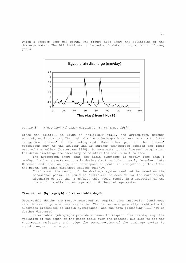
f - applying a correlation analysis (section 2.5) g - applying a segmented regression analysis (section 3). In this section only the following examples of time-series analysis will be given and their usefulness will be illustrated: - Time series (hydrograph) of drain discharge; - Time series (hydrograph) of water-table depth; - Frequency distributions in two sub-periods and differential mass method. Time series (hydrograph) of drain discharge Drain discharge is mostly measured at regular time intervals. Continuous records are only sometimes available. The latter are generally combined with automated procedures to obtain hydrographs, and the data processing will not be further discussed. Discharge hydrographs provide a means to inspect time-trends, e.g. the variation of discharge over the seasons, but also to see the short-term variations and judge the response-time of the drainage system to rapid changes in recharge. Figure 8 shows a hydrograph of pipe-drain discharges during the winter period (from November 1983 to March 1984) in the Mashtul drainage pilot area in the middle part of the Nile Valley, Egypt (DRI 1987). It concerns a unit in

22

which a berseem crop was grown. The figure also shows the salinities of the drainage water. The DRI institute collected such data during a period of many years.

Egypt, drain discharge (mm/day)

0

0.5

1

1.5

2

2.5

3

3.5

0 20 40 60 80 100 120 140 160

Time (days) from 1 Nov 83

Figure 8 Hydrograph of drain discharge, Egypt (DRI, 1987).

Since the rainfall in Egypt is negligibly small, the agriculture depends entirely on irrigation. The drain discharge hydrograph represents a part of the irrigation 'losses' to the underground. Some other part of the 'losses' percolates down to the aquifer and is further transported towards the lower part of the valley (Oosterbaan 1998). To some extent, the 'losses' originating the drain discharge are necessary to maintain the soil's salt balance The hydrograph shows that the drain discharge is mostly less than 1 mm/day. Discharge peaks occur only during short periods in early December, late December and late January, and correspond to peaks in irrigation gifts. After the peaks, the drain discharge reduces quickly. Conclusion: the design of the drainage system need not be based on the

occasional peaks. It would be sufficient to account for the more steady discharge of say than 1 mm/day. This would result in a reduction of the costs of installation and operation of the drainage system.

Time series (hydrograph) of water-table depth Water-table depths are mostly measured at regular time intervals. Continuous records are only sometimes available. The latter are generally combined with automated procedures to obtain hydrographs, and the data processing will not be further discussed. Water-table hydrographs provide a means to inspect time-trends, e.g. the variation of the depth of the water table over the seasons, but also to see the short-term variations and judge the response-time of the drainage system to rapid changes in recharge.

23

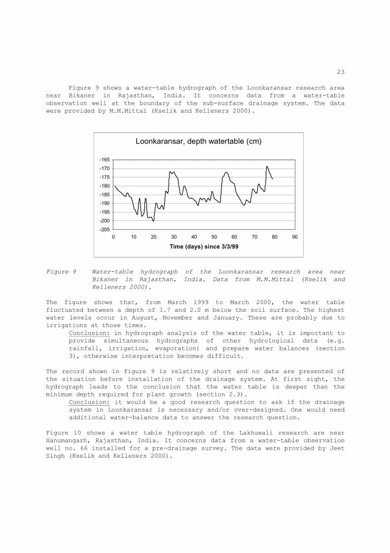
Figure 9 shows a water-table hydrograph of the Loonkaransar research area near Bikaner in Rajasthan, India. It concerns data from a water-table observation well at the boundary of the sub-surface drainage system. The data were provided by M.M.Mittal (Kselik and Kelleners 2000).

Loonkaransar, depth watertable (cm)

-205

-200

-195

-190

-185

-180

-175

-170

-165

0 10 20 30 40 50 60 70 80 90

Time (days) since 3/3/99

Figure 9 Water-table hydrograph of the Loonkaransar research area near

Bikaner in Rajasthan, India. Data from M.M.Mittal (Kselik and

Kelleners 2000).

The figure shows that, from March 1999 to March 2000, the water table fluctuated between a depth of 1.7 and 2.0 m below the soil surface. The highest water levels occur in August, November and January. These are probably due to irrigations at those times. Conclusion: in hydrograph analysis of the water table, it is important to

provide simultaneous hydrographs of other hydrological data (e.g. rainfall, irrigation, evaporation) and prepare water balances (section 3), otherwise interpretation becomes difficult.

The record shown in figure 9 is relatively short and no data are presented of the situation before installation of the drainage system. At first sight, the hydrograph leads to the conclusion that the water table is deeper than the minimum depth required for plant growth (section 2.3). Conclusion: it would be a good research question to ask if the drainage

system in Loonkaransar is necessary and/or over-designed. One would need additional water-balance data to answer the research question.

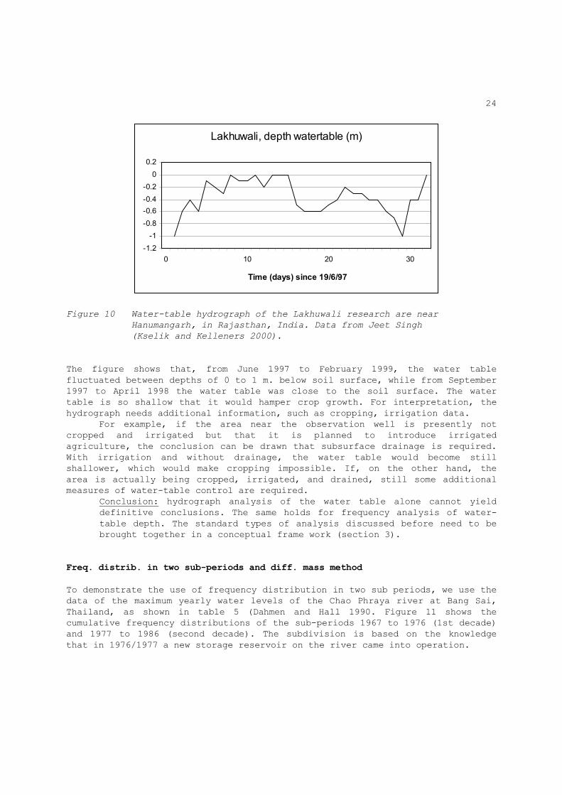
Figure 10 shows a water table hydrograph of the Lakhuwali research are near Hanumangarh, Rajasthan, India. It concerns data from a water-table observation well no. 66 installed for a pre-drainage survey. The data were provided by Jeet Singh (Kselik and Kelleners 2000).

24

Lakhuwali, depth watertable (m)

-1.2

-1

-0.8

-0.6

-0.4

-0.2

0

0.2

0 10 20 30

Time (days) since 19/6/97

Figure 10 Water-table hydrograph of the Lakhuwali research are near

Hanumangarh, in Rajasthan, India. Data from Jeet Singh

(Kselik and Kelleners 2000).

The figure shows that, from June 1997 to February 1999, the water table fluctuated between depths of 0 to 1 m. below soil surface, while from September 1997 to April 1998 the water table was close to the soil surface. The water table is so shallow that it would hamper crop growth. For interpretation, the hydrograph needs additional information, such as cropping, irrigation data. For example, if the area near the observation well is presently not cropped and irrigated but that it is planned to introduce irrigated agriculture, the conclusion can be drawn that subsurface drainage is required. With irrigation and without drainage, the water table would become still shallower, which would make cropping impossible. If, on the other hand, the area is actually being cropped, irrigated, and drained, still some additional measures of water-table control are required. Conclusion: hydrograph analysis of the water table alone cannot yield

definitive conclusions. The same holds for frequency analysis of water-table depth. The standard types of analysis discussed before need to be brought together in a conceptual frame work (section 3).

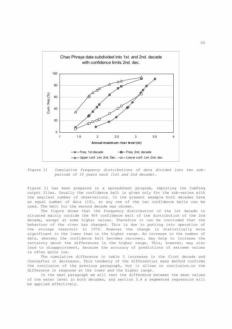
Freq. distrib. in two sub-periods and diff. mass method To demonstrate the use of frequency distribution in two sub periods, we use the data of the maximum yearly water levels of the Chao Phraya river at Bang Sai, Thailand, as shown in table 5 (Dahmen and Hall 1990. Figure 11 shows the cumulative frequency distributions of the sub-periods 1967 to 1976 (1st decade) and 1977 to 1986 (second decade). The subdivision is based on the knowledge that in 1976/1977 a new storage reservoir on the river came into operation.

25

Table 5. Maximum yearly water levels of the Chao Phraya river at Bang Sai, Thailand, and the cumulative differences from the mean (Dahmen and Hall 1990).

──────────────────────────────────────────────────────────── Year water level difference cumulative (H, m) H - Hav *) difference ----------------------------------------------------------- 1967 2.49 -0.004 -0.004 1968 2.80 0.306 0.302 1969 2.78 0.286 0.588 1970 1.95 -0.544 0.044 1971 3.29 0.796 0.840 1972 2.30 -0.194 0.646 1973 3.14 0.646 1.292 1974 3.20 0.706 1.998 1975 2.92 0.426 2.424 1976 3.51 1.016 3.440 1977 1.88 -0.614 2.826 1978 2.54 0.046 2.872 1979 1.98 -0.514 2.358 1980 1.42 -1.074 1.284 1981 2.63 0.136 1.420 1982 3.16 0.666 2.086 1983 1.78 -0.714 1.372 1984 1.76 -0.734 0.638 1985 2.04 -0.454 0.184 1986 2.31 -0.184 0.000 ──────────────────────────────────────────────────────────── *) Hav = 2.494 is the average value of H from 1967 to 1986

26

Chao Phraya data subdivided into 1st. and 2nd. decade

with confidence limits 2nd. dec.

0

20

40

60

80

100

1 1.5 2 2.5 3 3.5 4

Annual maximum river level (m)

Cum. freq (%)

Freq. 1st decade Freq. 2nd. decade

Upper conf. Lim. 2nd. Dec. Low er conf. Lim. 2nd. dec

Figure 11 Cumulative frequency distributions of data divided into two sub-

periods of 10 years each (1st and 2nd decade).

Figure 11 has been prepared in a spreadsheet program, importing the CumFreq output files. Usually the confidence belt is given only for the sub-series with the smallest number of observations. In the present example both decades have an equal number of data (10), so any one of the two confidence belts can be used. The belt for the second decade was chosen. The figure shows that the frequency distribution of the 1st decade is situated mainly outside the 90% confidence belt of the distribution of the 2nd decade, except at some higher values. Therefore it can be concluded that the behaviour of the river has changed. This is due to putting into operation of the storage reservoir in 1976. However the change is statistically more significant in the lower than in the higher range. An increase in the number of data, whereby the confidence belt becomes narrower, may help to increase the certainty about the differences in the higher range. This, however, may also lead to disappointment, because the accuracy of predictions of extreme values is often quite low. The cumulative difference in table 5 increases in the first decade and thereafter it decreases. This tendency of the differential mass method confirms the conclusion of the previous paragraph, but it allows no conclusion.on the difference in response at the lower and the higher range. In the next paragraph we will test the difference between the mean values of the water level in both decades, and section 3.4 a segmented regression will be applied effectively.

27

2.3 Testing of differences Instead of using frequency distributions of two sub-periods, one can also compare directly the difference (Dµ) between the mean values (µ1 and µ2 of the two distributions. In the previous example (water levels of the Chao Phraya river), the mean level of the 1st decade equals µ1 = 2.84 m and of the 2nd decade µ2 = 2.15 m so that Dµ = 2.84 - 2.15 = 0.69 m. The standard deviations are respectively σ1 = 0.48 m and σ2 = 0.51 m. The standard errors of the means are: S1 = σ1/√n1 S2 = σ2/√n2 where n1 and n2 are the number of data of the two series respectively. Thus, in the above example, we find that S1 = 0.48/√10 = 0.15 and S2 = 0.51/√10 = 0.16. Now, the standard error of the difference Dµ equals: Sd = √(S12+S22) so that, in this example, Sd = √(0.152+0.162) = 0.22 m. To test the statistical significance of the difference Dµ one needs to apply Student's test, using the statistic t that depends on the degrees of freedom (d) and the statistical risk (f) one accepts to reach the wrong conclusion (Table 6). The upper and lower confidence limits UD and VD of Dµ are: UD = Dµ + tSd (1a) VD = Dµ - tSd (1b) Since the risk f holds for both limits, the total risk equals 2f. For example, using an f-value of 0.05 (or 5%) implies a total risk of 10% The degrees of freedom depend on S1, S2, n1 and n2. When the differences between the S-values and n-values are relatively small, we can use by approximation: d = ns - 1 where ns is the smaller of the two n values. Using a risk of f = 0.05 (i.e. 5%), and the degrees of freedom d = 9, table 6 yields a t-value of 1.8.

28

Table 6 Values t of Student's distribution with d degrees of freedom and exceedance frequency f ────────────────────────────────────────────────────────────── d *) f=0.1 f=0.5 f=0.025 f=0.01 ------------------------------------------------------------- 5 1.48 2.02 2.57 3.37 6 1.44 1.94 2.45 3.14 7 1.42 1.90 2.37 3.00 8 1.40 1.86 2.31 2.90 9 1.39 1.83 2.26 2.82 10 1.38 1.81 2.22 2.76 12 1.36 1.78 2.18 2.68 14 1.35 1.76 2.15 2.62 16 1.34 1.75 2.12 2.58 20 1.33 1.73 2.09 2.53 25 1.32 1.71 2.06 2.49 30 1.31 1.70 2.04 2.45 40 1.30 1.68 2.02 2.42 60 1.30 1.67 2.00 2.39 100 1.29 1.66 1.99 2.37 200 1.28 1.65 1.97 2.35 ∞ 1.28 1.65 1.96 2.33 ────────────────────────────────────────────────────────────── *) For averages: d = n-1 (n = number of data) In linear regression: d = N-2 (N = number of pairs) In the given example we find: UD = 0.69 + 1.8 x 0.22 = 1.09 m and VD = 0.69 - 1.8 x 0.22 = 0.28 m. Expressing f in %, the (100-2f)% confidence interval (i.e. 100% certainty - 2f% risk) is: VD < Dµ < UD When VD and UD have the same sign (i.e. they are both positive or both negative) it is said that the difference Dµ is statistically significant at (100-2f)% level. In the case of our example the (100-2x5=90%) confidence interval is: 0.28 < Dµ < 1.09. Conclusion: there is a definite difference between the means µ1 and µ2.

However, from the frequency distributions of the two sub-periods, we have seen that at higher frequencies the differences between the higher water levels cannot be called statistically significant.

It is also concluded that what holds for the mean does not necessarily hold for the entire distribution.

29

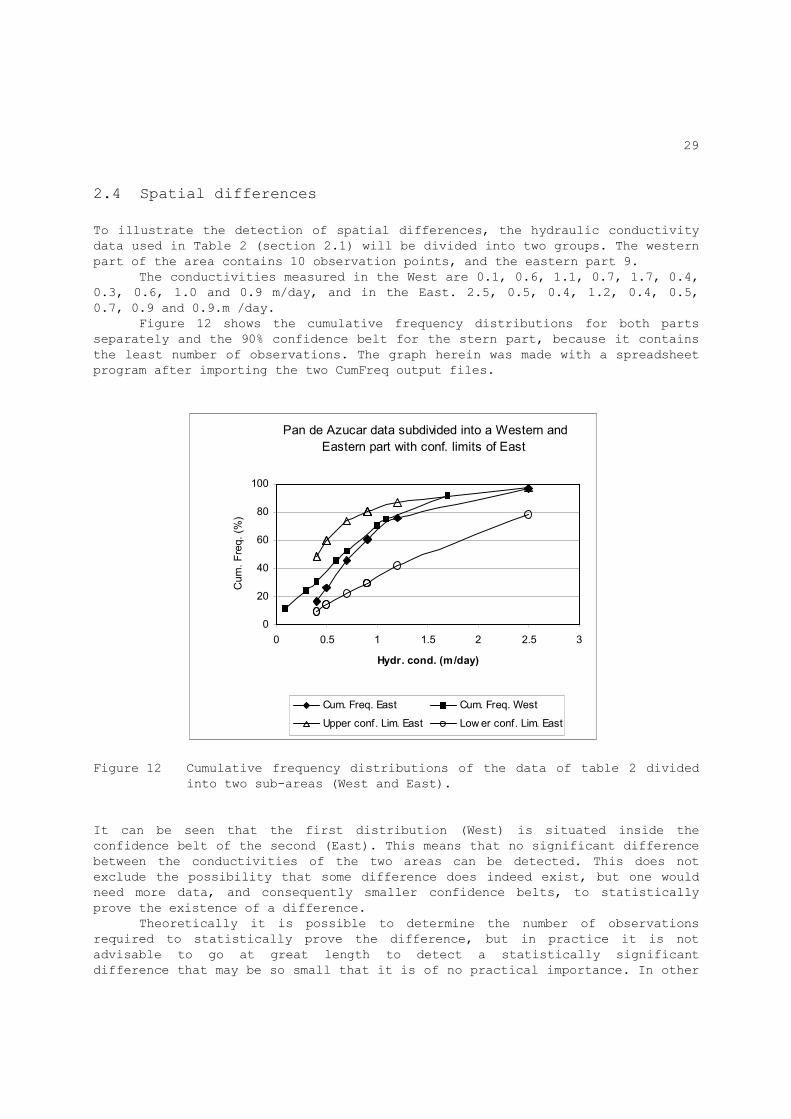
2.4 Spatial differences To illustrate the detection of spatial differences, the hydraulic conductivity data used in Table 2 (section 2.1) will be divided into two groups. The western part of the area contains 10 observation points, and the eastern part 9. The conductivities measured in the West are 0.1, 0.6, 1.1, 0.7, 1.7, 0.4, 0.3, 0.6, 1.0 and 0.9 m/day, and in the East. 2.5, 0.5, 0.4, 1.2, 0.4, 0.5, 0.7, 0.9 and 0.9.m /day. Figure 12 shows the cumulative frequency distributions for both parts separately and the 90% confidence belt for the stern part, because it contains the least number of observations. The graph herein was made with a spreadsheet program after importing the two CumFreq output files.

Pan de Azucar data subdivided into a Western and

Eastern part with conf. limits of East

0

20

40

60

80

100

0 0.5 1 1.5 2 2.5 3

Hydr. cond. (m/day)

Cum. Freq. (%

)

Cum. Freq. East Cum. Freq. West

Upper conf. Lim. East Lower conf. Lim. East

Figure 12 Cumulative frequency distributions of the data of table 2 divided

into two sub-areas (West and East). It can be seen that the first distribution (West) is situated inside the confidence belt of the second (East). This means that no significant difference between the conductivities of the two areas can be detected. This does not exclude the possibility that some difference does indeed exist, but one would need more data, and consequently smaller confidence belts, to statistically prove the existence of a difference. Theoretically it is possible to determine the number of observations required to statistically prove the difference, but in practice it is not advisable to go at great length to detect a statistically significant difference that may be so small that it is of no practical importance. In other

30

words, a statistically significant difference need not be physically significant, while a statistically insignificant difference is not necessarily physically insignificant. Only if there exists a significant physical difference that cannot be proven statistically, it is worthwhile to increase the number of observations. Instead of using frequency distributions, one can also compare directly the difference (Dµ) between the mean values of the distributions (section 2.3). In the above case the mean conductivity of the western part is µ1 = 0.74 m/day and of the eastern part µ2 = 0.89 m/day, so that Dµ = 0.74 - 0.89 = - 0.15. m/day. The standard deviations are respectively: σ1 = 0.46 and σ2 = 0.66 m/day while the number of data are: n1 = 10 and n2 = 9. The standard errors of the mean are: S1 = σ1/√n1 = 0.15 and S2 = σ2/√n2 = 0.22 m/day. Now, the standard error of the difference Dµ can be calculated as SD = √(S12+S22) = 0.27 m/day. The statistical significance of the difference Dµ is tested with Student's t-test described in section 2.3. Using a risk of f = 0.05 (i.e. 5%), and degrees of freedom d = 8, table 6 yields a t value of 1.8. The upper confidence limits UD of Dµ become Ud = Dµ + tSD = - 0.15 + 1.8 x 0.27 = + 0.34 It can be seen that the upper limit is positive, which indicates that there is a chance greater than 5% that UD>0. Hence the negative difference Dµ between µ1 and µ2 could have arisen by chance and might be positive instead. Conclusion: it is not quite possible to firmly decide which of the two µ

values is the greatest. A statistically significant difference at 5% confidence level does not exist.

It is also concluded that, in this example, a division into sub-areas with different conductivities cannot be recommended.

2.5 Correlation analysis The aim of correlation analysis is to detect a trend. In most spreadsheet programs, the correlation analysis is done as part of the linear regression analysis. In this section we discuss only the correlation coefficient. The regression analysis proper is applied in section 3, because it pre-supposes a concept of the regression model adopted. A trend between two variables may indicate that there is a cause-effect relation (direct correlation) or that there are one or more other factors, known or unknown, which affect the variables studied (indirect correlation). An intermediate situation is also possible. When direct correlation occurs, one can predict changes of a variable from changes in the other, irrespective whether these are natural or man-made changes (section 3)

31

When indirect correlation occurs, such predictions can only be made when the occurrences of the other influential factors are not systematically changed. Correlation is expressed in the correlation coefficient R or its squared value R2. It can be calculated conveniently with a computer spreadsheet program. The R-value ranges between -1 and +1. The value of R is + 1 when two variables (Y and X) investigated have a perfect positive linear relation, whereby Y increases proportionally to X. The R-value - 1 indicates a perfect negative linear relation, whereby Y decreases proportionally to X. When the two factors have absolutely no linear relation, the R factor is zero. Under the assumption of linearity, the R2 value gives the fraction of the squared values of the variations of one factor from its mean that can be explained by the other factor. A set of (Y,X) data pairs in which Y and X are not at all related may, by chance, still show a certain correlation. Various methods are available to test if the correlation is statistically significant. In section 3 we will be using the standard error of the regression coefficient for this purpose. The data of table 5 regarding the river levels and time, have a correlation R = - 0.40. It was proved earlier that the mean values of two sub-periods differ significantly. Hence, the coefficient R should also be significant. Figure 13 shows a picture of the yield of a wheat crop plotted against soil salinity (data from Sharma et al 1990). The frequency distributions of the data are shown in figures 1, 2 and 4. Calculation of the correlation coefficient with any appropriate computer program, e.g. a spreadsheet, gives a correlation value R = - 0.64. This indicates that the soil salinity negatively affects the crop yield and that a fraction R2 = 0.41 or 41% of the squared deviations of the yield Y can be explained by a linear regression upon the salinity X. The remaining deviations are due to other factors than X. This is understandable as the crop production is not only determined by salinity but by many other factors. However, from the relatively high correlation it can be concluded that the salinity plays a dominant role in the production. In section 6 it is shown that a segmented regression analysis yields important additional information.

32

Figure 13 Yield of a wheat crop plotted against soil salinity. (Data provided

by D.P.Sharma, CSSRI, Karnal, India, concerning farmers' fields in the Gohana area.). The data are the same as used in figures 1, 2, and 4.

33

3. Conceptual statistical analysis There are many forms of regression analysis e.g. linear versus non-linear, two-variable versus multi-variable, and ratio method versus least-squares method. The least squares method can be differentiated into regression of Y upon X, X upon Y, and intermediate regression. In addition, there are many different non-linear and multi-variable methods. In continuation, only linear, two-variable analyses will be presented. However, the possibilities of analysis will be extended by introducing: - Non-linearity made linear through transformation of data; - Non-linearity made linear through approximation by two linear

relations separated by a breakpoint (this segmentation method can also be applied to analyse mass curves and to find time trends);

- Multi-variability through sequential linear regressions. Linear regression by the ratio method presupposes that the scatter between the variables changes linearly with their value (dependent scatter). When independent scatter occurs, it is supposed to be normally distributed, and one can use the least-squares method. There are many methods of transforming data to obtain a linear relation. The most well known are the logarithmic transformations. In this case it is necessary to study the scatter of the transformed data before deciding whether to use the ratio or least squares method. Conceptual transformations, based on a theory of how one variable influences the other, can also be used. In the following sections the next subjects will be illustrated and discussed: - ratio method - linear regression of Y upon X, least squares method - linear regression with of Y upon X with zero intercept - conceptual transformation and linear regression of Y upon X with

zero intercept - linear regression of crop production on depth of water table - intermediate regression - segmented two-variable linear regression - successive segmented three-variable linear regressions

34

3.1 Linear regression, ratio method Linear 2-variable regression by the ratio method can be done when the scatter of the data depends on the magnitude of the Y and X values and Y = 0 when X = 0. An example of such a scatter diagram is shown in figure 14.

Figure 14 Plot of drain discharge (Q) versus hydraulic head (H) with

increasing scatter when Q and H increase The ratio (P) is expressed as: P = Y/X Its mean value is: - P = ΣP/N

where N is the number of (Y,X) data pairs. - The standard deviation of the ratio P is:

- 2 SP = √[Σ(P-P) /N(N-1)]

- A confidence interval of P can be made using the Student's statistic as explained in section 2.3:

35

- - Pu = P + t.SP

- - Pv = P - t.SP

- - - where Pu and Pv are the upper and lower confidence limits of P. - In the example of figure 14 we have: N = 18, P = 8.8 (mm/day/m), and SP = 0.42 (mm/day/m). Using a t-value of 1.75 for 90% confidence (table 6), we find: - - Pu = 9.5 and Pv = 8.1

The regression outcome can be used to estimate the soil's hydraulic conductivity using the Hooghoudt drainage equation, which, in its simplest form, reads: Q/H = 8KD/L2 where Q is the drain discharge (m/day), H is the height of the water table midway between the drains above drain level (m), KD is the soil's transmissivity (m2/day) and L is the drain spacing (m) we find the upper and lower confidence limits as: (8KD/L2)u = 0.0095 (8KD/L2)v = 0.0081 where a discharge conversion is made from mm/day to m/day. Assuming a drain spacing of L = 50 m, we find the 90% upper and lower confidence limits of the transmissivity KD as: KDu = 502 x 0.0095/8 = 2.97 m2day KDv = 502 x 0.0081/8 = 2.53 m2/day It is concluded that the KD value is determined with a relatively high degree of accuracy. Oosterbaan (1994) gives examples of adjustment of the ratio method when Y cannot be taken zero at X=0.

3.2 Linear regression, least squares method

36

The 2-variable linear regression by the least squares method can be done in two ways: regression of "Y upon X" and "X upon Y". With regression of Y upon X one determines a straight line of best fit minimising the square values of the Y-deviations (or Y- residuals) from the line. With regression of X upon Y one minimises the deviations in X-direction. When the squared correlation R2 is less than 1, the two regressions yield different results. Regression of Y upon X is to be done when X is an influential factor of Y. Then, Y is called the dependent and X the independent variable. When there is no direct causal relation between Y and X, one can do both the regression of Y upon X and X upon Y and determine an intermediate

regression coefficient. Linear regression analysis by the least squares method can be conveniently made with statistical or spreadsheet computer programs. The linear regression equation of Y upon X can be written as: ^ - - Yy = Ay(X-X) + Y

^ or Yy = AyX + Cy - - where Cy = Y - AyX

^ The symbol Yy indicates the value of Y calculated by regression of Y upon X. The factor Ay is called regression coefficient and represents the slope of the regression line. The Cy term is often called Y-intercept because it gives the ^ value of Y when X = 0. For regression of X upon Y we find similarly: ^ - - Xx = Ax(Y-Y) + X

^ or Xx = AxY + Cx - - where Cx = X - AxY

For comparison with the regression of Y upon X, the regression equation of X upon Y can be rewritten as: Y' = A'X + C' where A' = 1/Ax and - - C' = Y - A'X

37

It is often useful to calculate the standard errors of the coefficient A and intercept C to determine their confidence intervals and to detect their statistical significance. Most statistical and spreadsheet computer programs provide these standard errors automatically. If not, the following expressions can be used. We define the deviation or residual ε after regression of Y upon X as: ^ εy = Y - Y

Its mean value is zero. Its standard deviation is indicated by σεy and found from (σεy)

2 = Σ(εy)2/(N-2)

The standard error of coefficient Ay is indicated by SAy and found from: (SAy)

2 = (σεy/σX)2/(N-2)

The standard error of intercept Cy is indicated by SCy and found from: - (SCy)

2 = (AySX)2 + (XSAy)

2 In the above equations we used σX and SX as the standard deviation of X and the standard error of the mean value of X respectively (section 2.3). For regression of X upon Y a similar set of equations can mutatis mutandis be

used, by interchanging the symbols that need to be interchanged.

Below, the following examples of linear regression of Y upon X are given: - Linear relation between drain discharge and level of the water

table - Non-linear relation between drain discharge and level of the water

table linearised by conceptual transformation - Linear relation between crop production and depth of water table

38

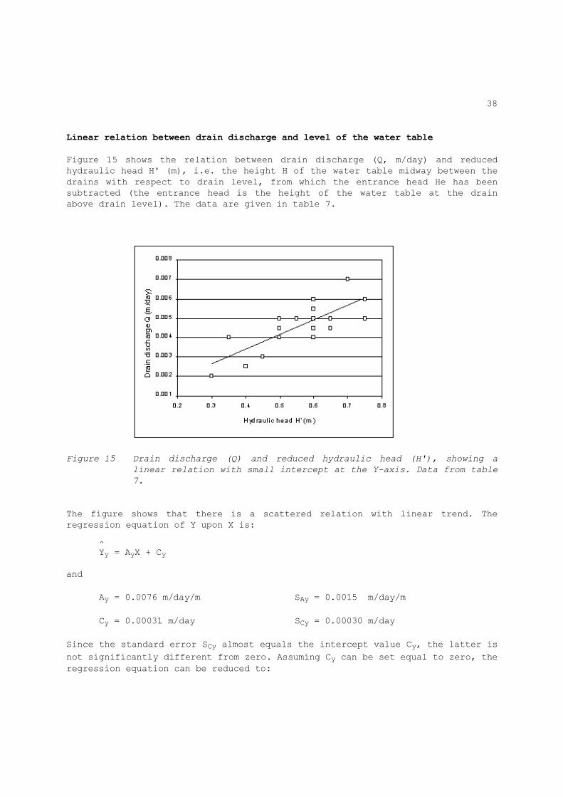
Linear relation between drain discharge and level of the water table Figure 15 shows the relation between drain discharge (Q, m/day) and reduced hydraulic head H' (m), i.e. the height H of the water table midway between the drains with respect to drain level, from which the entrance head He has been subtracted (the entrance head is the height of the water table at the drain above drain level). The data are given in table 7.

Figure 15 Drain discharge (Q) and reduced hydraulic head (H'), showing a

linear relation with small intercept at the Y-axis. Data from table

7.

The figure shows that there is a scattered relation with linear trend. The regression equation of Y upon X is: ^ Yy = AyX + Cy and Ay = 0.0076 m/day/m SAy = 0.0015 m/day/m Cy = 0.00031 m/day SCy = 0.00030 m/day Since the standard error SCy almost equals the intercept value Cy, the latter is not significantly different from zero. Assuming Cy can be set equal to zero, the regression equation can be reduced to:

39

Table 7. Drain discharge (Q), hydraulic head (H), entrance head (He) and reduced hydraulic head (H'=H-He). Data used in figure 15. ─────────────────────────────────────────── serial Q H He H' no. (m/day) (m) (m) (m) ------------------------------------------ 1 0.0020 0.31 0.01 0.30 2 0.0040 0.40 0.05 0.35 3 0.0025 0.50 0.10 0.40 4 0.0030 0.50 0.05 0.45 5 0.0045 0.70 0.20 0.50 6 0.0050 0.60 0.10 0.50 7 0.0040 0.55 0.05 0.50 8 0.0050 0.63 0.08 0.55 9 0.0050 0.72 0.12 0.60 10 0.0055 0.70 0.10 0.60 11 0.0060 0.80 0.20 0.60 12 0.0045 0.75 0.15 0.60 13 0.0040 0.85 0.25 0.60 14 0.0050 0.70 0.05 0.65 15 0.0045 0.75 0.10 0.65 16 0.0070 0.85 0.15 0.70 17 0.0060 0.95 0.20 0.75 18 0.0050 0.90 0.15 0.75 ─────────────────────────────────────────── ^ Yy = 0.0076 X Now the determination of the soil's transmissivity can proceed along the lines

discussed in section 3.1 replacing the ratio P by the slope Ay.

When neglecting the intercept, one can alternatively calculate the slope Ay from: - - Ay = Y/X

- - In this example we have Y = 0.00458 and X = 0.558 so that Ay = 0.0082. The difference with the previous value of Ay is less than 8% and small compared to the relative standard error (calculated as 100 x 0.0015 / 0.0076 = 20%). Thus, the alternative is acceptable. However, when neglecting the intercept Cy, the standard errors become wider because the sum of the residuals will be more, but, when Cy is insignificant, the difference in standard error is negligibly small and we can use the standard errors as calculated from the standard regression analysis.

40

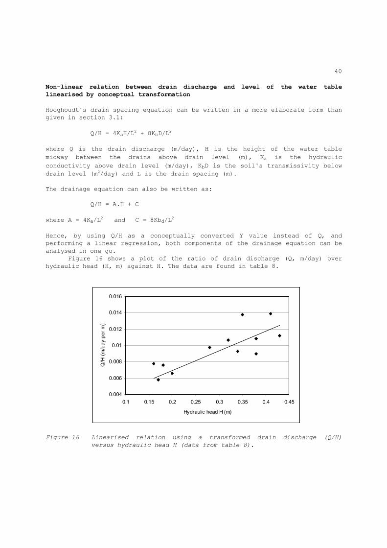
Non-linear relation between drain discharge and level of the water table

linearised by conceptual transformation Hooghoudt's drain spacing equation can be written in a more elaborate form than given in section 3.1: Q/H = 4KaH/L2 + 8KbD/L2 where Q is the drain discharge (m/day), H is the height of the water table midway between the drains above drain level (m), Ka is the hydraulic conductivity above drain level (m/day), KbD is the soil's transmissivity below drain level (m2/day) and L is the drain spacing (m). The drainage equation can also be written as: Q/H = A.H + C where A = 4Ka/L2 and C = 8Kbd/L2 Hence, by using Q/H as a conceptually converted Y value instead of Q, and performing a linear regression, both components of the drainage equation can be analysed in one go. Figure 16 shows a plot of the ratio of drain discharge (Q, m/day) over hydraulic head (H, m) against H. The data are found in table 8.

0.004

0.006

0.008

0.01

0.012

0.014

0.016

0.1 0.15 0.2 0.25 0.3 0.35 0.4 0.45

Hydraulic head H (m)

Q/H

(m/day per m)

Figure 16 Linearised relation using a transformed drain discharge (Q/H)

versus hydraulic head H (data from table 8).

41

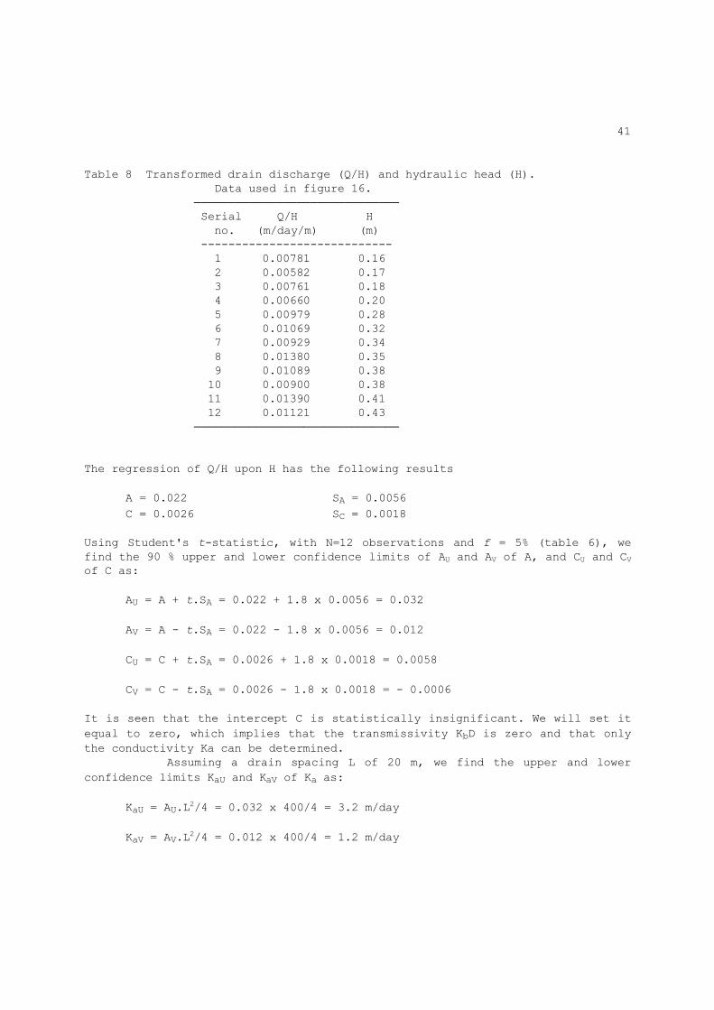
Table 8 Transformed drain discharge (Q/H) and hydraulic head (H). Data used in figure 16. ────────────────────────────── Serial Q/H H no. (m/day/m) (m) ---------------------------- 1 0.00781 0.16 2 0.00582 0.17 3 0.00761 0.18 4 0.00660 0.20 5 0.00979 0.28 6 0.01069 0.32 7 0.00929 0.34 8 0.01380 0.35 9 0.01089 0.38 10 0.00900 0.38 11 0.01390 0.41 12 0.01121 0.43 ────────────────────────────── The regression of Q/H upon H has the following results A = 0.022 SA = 0.0056 C = 0.0026 SC = 0.0018 Using Student's t-statistic, with N=12 observations and f = 5% (table 6), we find the 90 % upper and lower confidence limits of AU and AV of A, and CU and CV of C as: AU = A + t.SA = 0.022 + 1.8 x 0.0056 = 0.032 AV = A - t.SA = 0.022 - 1.8 x 0.0056 = 0.012 CU = C + t.SA = 0.0026 + 1.8 x 0.0018 = 0.0058 CV = C - t.SA = 0.0026 - 1.8 x 0.0018 = - 0.0006 It is seen that the intercept C is statistically insignificant. We will set it equal to zero, which implies that the transmissivity KbD is zero and that only the conductivity Ka can be determined. Assuming a drain spacing L of 20 m, we find the upper and lower confidence limits KaU and KaV of Ka as: KaU = AU.L2/4 = 0.032 x 400/4 = 3.2 m/day KaV = AV.L2/4 = 0.012 x 400/4 = 1.2 m/day

42

Due to omitting the intercept C, the above confidence limits may be slightly wider than calculated here. However, when C is insignificant, the difference will be negligibly small. Due to the scatter of data and the limited number of observations, the confidence interval of Ka is relatively wide, but narrower than one would find with direct hydraulic conductivity tests as analysed in figure 5 and also as observed by Oosterbaan and Nijland (1994). Conclusion: relatively high accuracy, a larger number of observations is

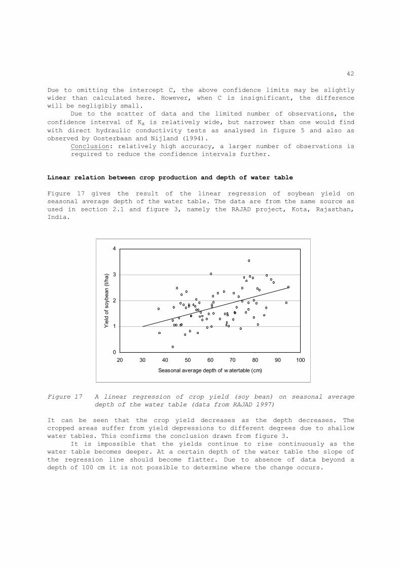
required to reduce the confidence intervals further. Linear relation between crop production and depth of water table Figure 17 gives the result of the linear regression of soybean yield on seasonal average depth of the water table. The data are from the same source as used in section 2.1 and figure 3, namely the RAJAD project, Kota, Rajasthan, India.

0

1

2

3

4

20 30 40 50 60 70 80 90 100

Seasonal average depth of w atertable (cm)

Yield of soybean (t/ha)

Figure 17 A linear regression of crop yield (soy bean) on seasonal average

depth of the water table (data from RAJAD 1997)

It can be seen that the crop yield decreases as the depth decreases. The cropped areas suffer from yield depressions to different degrees due to shallow water tables. This confirms the conclusion drawn from figure 3. It is impossible that the yields continue to rise continuously as the water table becomes deeper. At a certain depth of the water table the slope of the regression line should become flatter. Due to absence of data beyond a depth of 100 cm it is not possible to determine where the change occurs.

43

Conclusion: from the fact that deep enough water tables have not been observed in this random sample in farmer's fields, it can be concluded that the major part of the area does not have the water table at a safe depth.

The value of the regression coefficient is Ay = 0.0203 indicating that the yield decreases with about 0.02 t/ha for each cm decrease of the water-table depth. The number of data pairs amounts to 82 and the standard error of the regression coefficient is SAy = 0.00396. A significance test using Student's t-statistic (section 2.3) will reveal that the coefficient is statistically highly significant. The period of growth of soybean in the RAJAD project is the monsoon season with high rainfall. The areas in which the soybean yields have been determined were equipped with a subsurface drainage system. The system was designed for salinity control and water-table control outside the monsoon. Water-table control during the monsoon season would make the drainage system more costly. Apparently, the yield depression of soybean has been accepted as unavoidable. Assuming that the agricultural sector is not content with this situation, one could either grow another crop that can withstand higher levels of the water table, or one could try to demonstrate that the benefit of intensifying the drainage system would justify the additional cost of better water-table control during monsoon. Assuming that an intensified drainage system is able to maintain the seasonal average depth of the water table at 100 cm, the average yield increase (Yi) can be estimated from: - Yi = Ay(100-X) In the example we would get Yi = 0.02 (100 - 64) = 0.72 t/ha per year. Conclusion: in the example, the linear regression analysis permits to

assess the yield increase from intensified drainage. In an economic cost-benefit analysis one could assess if this would warrant the drainage intensification.

Later we will see that a segmented linear regression shows that the water-table requirements can be reduced so that the same effect is obtained with a lower investment.

44

3.3 Intermediate regression It is advisable to use the intermediate regression when the Y and X data are not mutually influential and one is not interested in predicting the value of one of the two variables from the other but rather in determining the value of parameters, such as regression coefficient (A) and Y-intercept (C). For intermediate regression one performs the regression of Y upon X and X upon Y as discussed in section 3.2. Thereafter one determines the intermediate regression coefficient A* from the geometric mean of the regression coefficients Ay and A'=1/Ax as: A* = √(AyA') The standard error SA* of A* can be calculated using the principle that its relative value to A* is equal to the relative value of the standard error SAy of Ay to Ay itself and of the standard error SAx of Ax to Ax: SA* = A*SAy/Ay = A*SAx/Ax The Y-intercept C* of the intermediate regression line is found from: - - C* = Y - A*X

The standard error of SC* of C* can be calculated by: - SC* = √[(A*SX)

2+(XSA*)2]

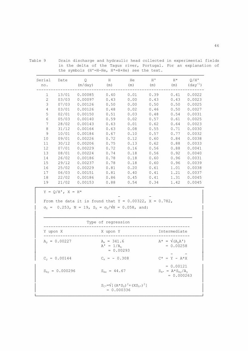
To illustrate the intermediate regression, we use data collected in an experimental field in the delta of the Tagus river, Portugal (table 9, figure 18). The data were obtained during a period of recession of the water table after recharge by rain had occurred. The subsurface drains are spaced at a distance of 20 m. Oosterbaan and Nijland (1994) have presented an adjusted Hooghoudt equation to analyse the receding water table under influence of a sub-surface drainage system with entrance resistance: Q/H' = 2πKbd/L2 + πKaH*/L2 with: H' = H-He H* = H+He where Q is the drain discharge (m/day), H is the hydraulic head or height of the water table midway between the drains with respect to drain level (m), He is the entrance head or height of the water table at the drain with respect to

45

drain level (m) Kb is the hydraulic conductivity of the soil below drain level (m/day), Ka is the hydraulic conductivity of the soil above drain level (m/day), d is Hooghoudt's equivalent depth of an impermeable layer below drain level (m), and L is the drain spacing (m). For the determination of the equivalent depth reference is made to Ritzema (1994). To find the values of Kbd and Ka we need to do an intermediate regression of Y upon X, or in this case of Q/H upon H*, to obtain: Y = Q/H' = C* + A*X = C* + A*H* C* = 2πKbd/L2 A* = πKa/L* The results of the intermediate regression are given in table 9 and figure 18. Thus we determine the expected hydraulic conductivities according to regression as follows: C* = 2πKbd/L2 = 0.00122, and Kbd = 0.00122 L2/2π = 0.078 m2/day A* = πKa/L2 = 0.00258, and Ka = 0.00258 L2/π = 0.329

46

Table 9 Drain discharge and hydraulic head collected in experimental fields

in the delta of the Tagus river, Portugal. For an explanation of the symbols (H'=H-He, H*=H+He) see the text.

────────────────────────────────────────────────────────────────────── Serial Date Q H He H' H* Q/H' no. (m/day) (m) (m) (m) (m) (day-1) ---------------------------------------------------------------------- 1 13/01 0.00085 0.40 0.01 0.39 0.41 0.0022 2 03/03 0.00097 0.43 0.00 0.43 0.43 0.0023 3 07/03 0.00126 0.50 0.00 0.50 0.50 0.0025 4 03/01 0.00126 0.48 0.02 0.46 0.50 0.0027 5 02/01 0.00150 0.51 0.03 0.48 0.54 0.0031 6 05/03 0.00140 0.59 0.02 0.57 0.61 0.0025 7 28/02 0.00143 0.63 0.01 0.62 0.64 0.0023 8 31/12 0.00164 0.63 0.08 0.55 0.71 0.0030 9 10/01 0.00184 0.67 0.10 0.57 0.77 0.0032 10 09/01 0.00226 0.72 0.12 0.60 0.84 0.0038 11 30/12 0.00206 0.75 0.13 0.62 0.88 0.0033 12 07/01 0.00229 0.72 0.16 0.56 0.88 0.0041 13 08/01 0.00224 0.74 0.18 0.56 0.92 0.0040 14 26/02 0.00186 0.78 0.18 0.60 0.96 0.0031 15 29/12 0.00237 0.78 0.18 0.60 0.96 0.0039 16 25/02 0.00229 0.81 0.20 0.61 1.01 0.0038 17 06/03 0.00151 0.81 0.40 0.41 1.21 0.0037 18 22/02 0.00186 0.86 0.45 0.41 1.31 0.0045 19 21/02 0.00153 0.88 0.54 0.34 1.42 0.0045 ┌────────────────────────────────────────────────────────────────────── │ Y = Q/H', X = H* │ │ - - │ │ From the data it is found that Y = 0.00322, X = 0.782, │

│ σX = 0.253, N = 19, SX = σX/√N = 0.058, and: │ │ │ │ ────────────────────────────────────────────────────────────── │ │ Type of regression │ │ ------------------------------------------------------------- │ │ Y upon X X upon Y Intermediate │ │ ------------------------------------------------------------- │ │ Ay = 0.00227 Ax = 341.6 A* = √(AyA') │ │ A' = 1/Ax = 0.00258 │ │ = 0.00293 │ │ - - │ │ Cy = 0.00144 Cx = - 0.308 C* = Y - A*X │

│ = 0.00121 │ │ SAy = 0.000296 SAx = 44.67 SA* = A*SAy/Ay │ │ = 0.000263 │ │ │ │ SC*=√[(A*SX)2+(XSA*)2] │ │ = 0.000336 │

└─────────────────────────────────────────────────────────────────────┘

47

Data from drainage pilot area in Tagus delta, Portugal

0.0015

0.0025

0.0035

0.0045

0.0055

0.0065

0.3 0.5 0.7 0.9 1.1 1.3 1.5 1.7

Adjusted hydr. head (m)

Discharge head ratio Q

/H' (m

/day/m

)

observed intermediate Y upon X X upon Y

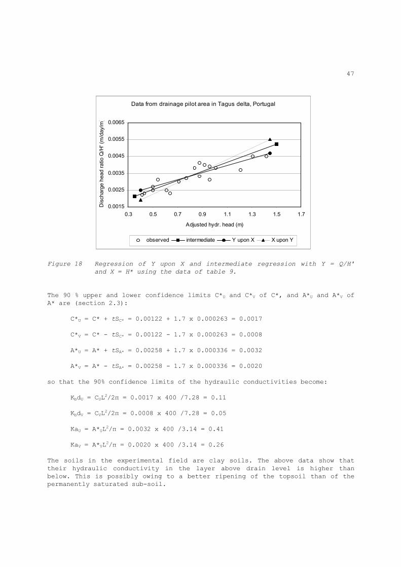
Figure 18 Regression of Y upon X and intermediate regression with Y = Q/H'

and X = H* using the data of table 9.

The 90 % upper and lower confidence limits C*U and C*V of C*, and A*U and A*V of A* are (section 2.3): C*U = C* + tSC* = 0.00122 + 1.7 x 0.000263 = 0.0017 C*V = C* - tSC* = 0.00122 - 1.7 x 0.000263 = 0.0008 A*U = A* + tSA* = 0.00258 + 1.7 x 0.000336 = 0.0032 A*V = A* - tSA* = 0.00258 - 1.7 x 0.000336 = 0.0020 so that the 90% confidence limits of the hydraulic conductivities become: KbdU = CUL2/2π = 0.0017 x 400 /7.28 = 0.11 KbdV = CVL2/2π = 0.0008 x 400 /7.28 = 0.05 KaU = A*UL2/π = 0.0032 x 400 /3.14 = 0.41 KaV = A*VL2/π = 0.0020 x 400 /3.14 = 0.26 The soils in the experimental field are clay soils. The above data show that their hydraulic conductivity in the layer above drain level is higher than below. This is possibly owing to a better ripening of the topsoil than of the permanently saturated sub-soil.

48

3.4 Segmented two-variable linear regression Segmented linear regression is done by performing separate linear regressions to the data with X values smaller and greater than a certain separation value: the break point. One can say: regression is done separately to the left and to the right of the break point. Figure 19 illustrates some of the trends that can be detected with segmented linear regression. The trends, represented by broken lines, can be considered representative of various types of logarithmic, exponential and parabolic curves. Often the scatter of data is so large that the fitting of smooth curves through the data suggests a higher degree of accuracy than is actually existing. Segmented linear regression is often good enough for the purpose, it gives results that can be easily checked by the researcher, and it offers the advantage of being able to dividing the database into two different collections of data with different characteristics. Segmented linear regression makes it possible to devise criteria, based on the confidence intervals of the parameters of the linear relations, enabling us to classify non-linear relations into such types as depicted in figure 19. The SegReg (see www.waterlog.info/segreg.htm ) computer program uses such criteria. In addition to the types of confidence analysis discussed before in this chapter, an important decisive criterion factor is the coefficient of

explanation (E). Neglecting a small correction for degrees of freedom, it can be defined as: ^ 2 2 Σ(Y-Y) Σ ε 2 2 E = 1 - ─────── = 1 - ───── = 1 - Sε/Sy - 2 2 Σ(Y-Y) Σ δ

It can be seen that E = 1 when Σε2 = 0, i.e. all the original variation in Y has been removed and no residual variation is left: there is a perfect match between the regression model and the data, the model explains all the variations. On the other hand, we see that E = 0 when Σε2 = Σδ2, meaning that after application of the regression model the variation of the residuals is as large as the original variation in Y: there has been no explanation at all. In linear regression without break point, the coefficient E is equal to the correlation coefficient R. However, in non-linear or segmented regression the two coefficients may be different and the R coefficient loses some of its meaning. Yet, in segmented regression it will be required to check that the segmentation does not yield a smaller explanation coefficient than the correlation coefficient. The SegReg program assumes a range of break-point values from which the one with the highest explanation is selected.

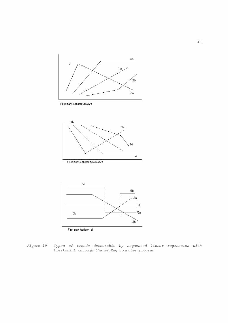
49

Figure 19 Types of trends detectable by segmented linear regression with

breakpoint through the SegReg computer program

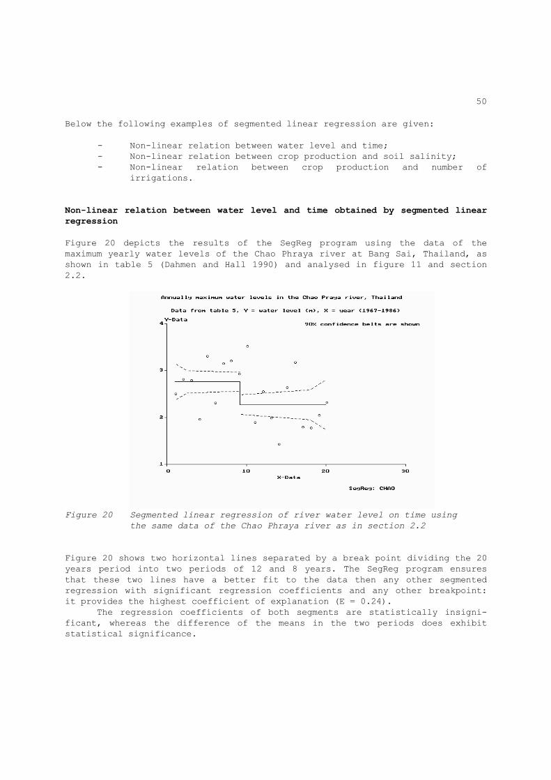
50

Below the following examples of segmented linear regression are given: - Non-linear relation between water level and time; - Non-linear relation between crop production and soil salinity; - Non-linear relation between crop production and number of

irrigations. Non-linear relation between water level and time obtained by segmented linear

regression Figure 20 depicts the results of the SegReg program using the data of the maximum yearly water levels of the Chao Phraya river at Bang Sai, Thailand, as shown in table 5 (Dahmen and Hall 1990) and analysed in figure 11 and section 2.2.

Figure 20 Segmented linear regression of river water level on time using

the same data of the Chao Phraya river as in section 2.2

Figure 20 shows two horizontal lines separated by a break point dividing the 20 years period into two periods of 12 and 8 years. The SegReg program ensures that these two lines have a better fit to the data then any other segmented regression with significant regression coefficients and any other breakpoint: it provides the highest coefficient of explanation (E = 0.24). The regression coefficients of both segments are statistically insigni-ficant, whereas the difference of the means in the two periods does exhibit statistical significance.

51

Conclusion: the segmented regression provides additional information to the methods of analysis discussed before and clearly shows that there is a sudden, one-time, change in the time series of water level. The breakpoint occurs at the 11th year.

Non-linear relation between crop production and soil salinity obtained by

segmented linear regression Figure 21 depicts the segmented linear regression of the yield of a wheat crop upon soil salinity (Sharma et al. 1990). The data were used before in section 2.5 (correlation analysis) and figure 13.

Figure 21 Segmented linear regression analysis of wheat yield against soil

salinity in farmers' fields of the Gohana area, Haryana, India. The

analysis is done with the SegReg computer program using the same

database as in figures 1, 2, 4, and 13.

Figure 21, prepared with the SegReg program, clearly shows that the wheat yield is independent of soil salinity up to a salinity value of EC = 5 dS/m (the break-point, Bp, or threshold). Here, the graph shows a horizontal line, and the regression coefficient is statistically insignificant. Beyond the breakpoint (Bp = 5 dS/m), the relation has a statistically significant downward sloping trend and the crop yields are declining on average at a rate of AyX>Bp = 0.28 t/ha per EC unit of 1 dS/m. The 90% confidence interval of the breakpoint is relatively narrow: it ranges between 3 and 6. A somewhat wider confidence interval is noticeable in figure 22 concerning the relation between the yield of mustard and soil

52

salinity (Oosterbaan et al. 1990). Still, the breakpoint is significantly larger than zero. The broken line of figure 21 has an explanation coefficient E = 0.44, which is higher than the correlation coefficient R2 = 0.41. This indicates that the broken line has a better fit with the data than the best fitting straight line without a break point. The SegReg program provides all other statistical data necessary to substantiate the conclusions, including a confidence area or confidence block of the breakpoint. From the fraction of the X-data with salinity values greater than Bp = 5 dS/m, one can estimate the percentage of the area suffering from a decline of crop yield due to high salinity. In this example, the fraction amounts to FX>Bp = 0.42 or 42% Supposing one is able to undertake a land reclamation project so that the soil salinity is maintained at a safe level of Bp = 5 dS/m or less, then one can expect an increase of wheat production of: - - Yi = FX>Bp(YX>Bp-YX<Bp) = 0.42(3.67-2.70) = 0.41 t/ha per year The SegReg program prints the standard errors of the estimates of area fraction affected and yield increase expected from a reclamation project (in this example respectively 4.9 % and 0.085 t/ha), so that the confidence limits of the estimates can be calculated using Student's t-test (section 2.3). The estimates are highly significant. Conclusion: compared to a correlation analysis, an un-segmented linear

regression analysis provides important additional information, including a threshold value and information of economical importance, on the basis of which quantitative recommendations for land reclamation and salinity control can be formulated.

53

Figure 22 Segmented linear regression analysis of mustard yield against soil

salinity in experimental fields of the Sampla pilot area, Haryana,

India. The analysis is done with the SegReg computer program.

Note: for additional information on crop salt tolerance see article on website: www.waterlog.info/pdf/segmregr.pdf Non-linear relation between crop production and number of irrigations analysed

by segmented linear regression The database used in the previous example also contains data on number of irrigations, so that the relation between wheat production and irrigation can be established. The "warabandi" irrigation system in Haryana state, India, allows a certain number of irrigations during the growing season. Each irrigation brings about 75 mm of water to the crop. For a winter crop like wheat the number irrigations varies between 1 and 4. Figure 23 shows the outcome of the SegReg program. Despite the fact that the number of irrigations is a discrete variable, not continuous as soil salinity, it is possible to draw definite conclusions. The main conclusion is that the effect of the first three irrigations is limited, only the fourth irrigation produces an improved yield.

54

Figure 23 Segmented linear regression analysis of wheat yield against number

of irrigations in farmers' fields of the Gohana area, Haryana,

India. The analysis is done with the SegReg computer program using

the same database as in figure 1, 2, 4, 13, 21 and 23.

The apparently limited impact of irrigation number 2 and 3 is perhaps due to some compensation in the form of additional irrigation by ground water through informal tube wells. The quantity of tube well irrigation is not known. If it would be true that tube well irrigation is practised, then the number of irrigations is not entirely representative for the amount of irrigation water applied, and the effect of the formal irrigations would be obscured. When discrete variables (numbers) are used, the confidence limits of the break point need an interpretation. In this example they indicate that the breakpoint is significantly greater than 2 and significantly less than 4, hence it is significantly 3. Non-linear relation between crop production and depth of water table analysed

by segmented linear regression The linear analysis applied to crop yield and depth of water table in figure 17 can be extended to non-linear analysis. The result is shown in figure 24.

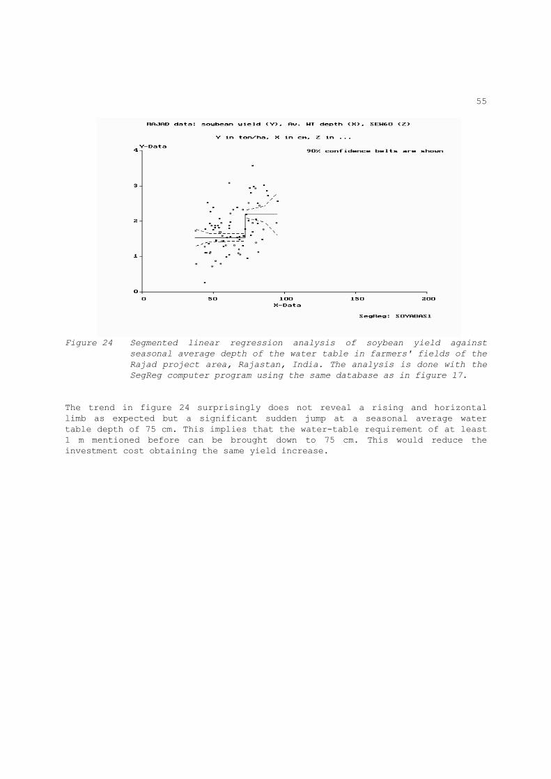
55

Figure 24 Segmented linear regression analysis of soybean yield against

seasonal average depth of the water table in farmers' fields of the

Rajad project area, Rajastan, India. The analysis is done with the

SegReg computer program using the same database as in figure 17.

The trend in figure 24 surprisingly does not reveal a rising and horizontal limb as expected but a significant sudden jump at a seasonal average water table depth of 75 cm. This implies that the water-table requirement of at least 1 m mentioned before can be brought down to 75 cm. This would reduce the investment cost obtaining the same yield increase.

56

3.5 Segmented three-variable linear regression The database on wheat production (Y) used before contains two independent variables X (soil salinity) and Z (number of irrigations). The SegReg program offers the possibility to perform the successive regression on both variables. The program will first do the segmented regression on the variable giving the higher coefficient of explanation (E) and calculates the Y-residuals, indicated by YXr or YZr depending on whether the X or Z variable was taken first. In the wheat database, the higher E-coefficient (0.44) is given by the soil salinity (X), with break point BPx = 5 Ds/m. Hence, the YXr residuals are determined first and then a segmented regression is made on Z (figure 25). In total four regression equations result: when X<BPx and Z<BPz : Y = As.X + Bs.Z + Css when X<BPx and Z>BPz : Y = As.X + Bg.Z + Csg when X>BPx and Z<BPz : Y = Ag.X + Bs.Z + Cgs when X>BPx and Z>BPz : Y = Ag.X + Bg.Z + Cgg The values of the parameters and other statistical information on the sequential three-variable regression of the wheat data are given in table 10. It can be seen that the total coefficient of explanation has risen to E = 0.51. From table 11 it can be seen that the salinity X and the number Z are un-correlated. When the two independent variables are strongly correlated one will find that the second variable will not contribute much to the explanation of the variations after the first has been used. Figure 26 depicts a plot of the observed and calculated wheat yields after the sequential regressions, showing that still a considerable variation is unexplained by the two independent variables used. Agricultural production is determined by many more factors.

57

Figure 25 Segmented linear regression analysis of the residuals of the wheat

yield remaining after regression upon soil salinity, against number

of irrigations in farmers' fields of the Gohana area, Haryana,

India. The analysis is done with the SegReg computer program using

the same database as in figures 1, 2, 4, 13, 21, 23, and 25.

Figure 26 Observed and calculated wheat yields after sequential segmented

regression upon soil salinity and number of irrigations in farmers'

fields of the Gohana area, Haryana, India. The analysis is done

with the SegReg computer program using the same database as in

figures 1, 2, 4, 13, 21, 23, 26, and 25.

58

Table 10 Summary of outcomes of the SegReg program after the sequential segmented

regression analysis of wheat on soil salinity and number of irrigations, using the same database as in figures 13, 21, 23, 25, and 26.

┌──────────────────────────────────────────────────────────────────┐ │GOHANA DATA wheat yield (Y), soil salinity (X) and No. of irr. (Z)│ │Y in ton/ha, X in EC (dS/m), Z (-) │ │ │ │Regression of Y upon X without breakpoint (BPx=0). │ │The table below gives the following series of values respectively │ │ Breakpoint(BPx) number of data Av.Y Av.X │ │ regr.coeff.(rc) corr.coeff.sq. st.dev.rc Y(X=0) │ │ st.dev.Y st.dev.YXr st.dev.X │ │ │ │BPx= .00 .100E+03 .326E+01 .539E+01 │ │ -.175E+00 .409E+00 .213E-01 .421E+01 │ │ .914E+00 .702E+00 .333E+01 │ │ │ │Results of regression of Y upon X with optimal breakpoint (BPx) │ │(giving better results than the similar regression of Y upon Z). │ │The table below gives the following series of values respectively │ │ Breakpoint(BPx) number of data Av.Y Av.X │ │ regr.coeff.(rc) corr.coeff.sq. st.dev.rc Y(X=0) │ │ st.dev.Y st.dev.YXr st.dev.X │ │for the data with X-values smaller and greater than BPx, followed │ │by function parameters. │ │ │ │Data with X < BPx: │ │BPx= 5.00 .580E+02 .367E+01 .312E+01 │ │ .107E-01 .378E-03 .737E-01 .364E+01 │ │ .672E+00 .672E+00 .122E+01 │ │Data with X > BPx: │ │BPx= 5.00 .420E+02 .270E+01 .852E+01 │ │ -.214E+00 .416E+00 .401E-01 .452E+01 │ │ .906E+00 .692E+00 .273E+01 │ │ │ │Parameters for function type 3 and method 2 (see manual) : │ │ slope (>BPx) Ybp N>/Nt increase Yi│ │ -.278E+00 .367E+01 .420E+00 .410E+00 │ │ st.err.slope st.err.BPx st.err.N>/Nt st.err.Yi │ │ .414E-01 .732E+00 .494E-01 .846E-01 │ │ st.dev.YXr (>BPx) st.dev.Ybp expl.coeff. │ │ .714E+00 .883E-01 .436E+00 │ │ │ │Regression of X upon Z without breakpoint (BPx=0) │ │(to show the correlation between the two independent variables). │ │The table below gives the following series of values respectively │ │ Breakpoint(BPz) number of data Av.X Av.Z │ │ regr.coeff.(rc) corr.coeff.sq. st.dev.rc X(Z=0) │ │ st.dev.X st.dev.XZr st.dev.Z │ │ │ │BPz= .00 .100E+03 .539E+01 .285E+01 │ │ -.355E+00 .581E-02 .469E+00 .640E+01 │ │ .333E+01 .332E+01 .716E+00 │ │ │ │ │ continued

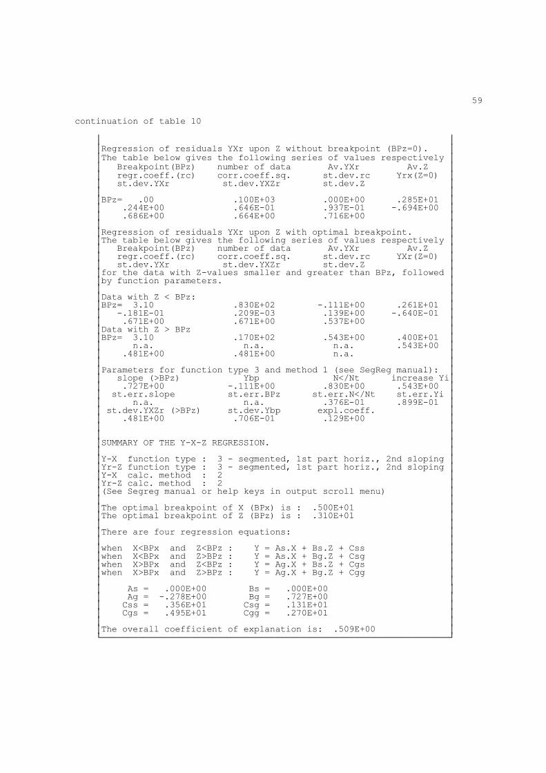
59

continuation of table 10 │ │ │Regression of residuals YXr upon Z without breakpoint (BPz=0). │ │The table below gives the following series of values respectively │ │ Breakpoint(BPz) number of data Av.YXr Av.Z │ │ regr.coeff.(rc) corr.coeff.sq. st.dev.rc Yrx(Z=0) │ │ st.dev.YXr st.dev.YXZr st.dev.Z │ │ │ │BPz= .00 .100E+03 .000E+00 .285E+01 │ │ .244E+00 .646E-01 .937E-01 -.694E+00 │ │ .686E+00 .664E+00 .716E+00 │ │ │ │Regression of residuals YXr upon Z with optimal breakpoint. │ │The table below gives the following series of values respectively │ │ Breakpoint(BPz) number of data Av.YXr Av.Z │ │ regr.coeff.(rc) corr.coeff.sq. st.dev.rc YXr(Z=0) │ │ st.dev.YXr st.dev.YXZr st.dev.Z │ │for the data with Z-values smaller and greater than BPz, followed │ │by function parameters. │ │ │ │Data with Z < BPz: │ │BPz= 3.10 .830E+02 -.111E+00 .261E+01 │ │ -.181E-01 .209E-03 .139E+00 -.640E-01 │ │ .671E+00 .671E+00 .537E+00 │ │Data with Z > BPz │ │BPz= 3.10 .170E+02 .543E+00 .400E+01 │ │ n.a. n.a. n.a. .543E+00 │ │ .481E+00 .481E+00 n.a. │ │ │ │Parameters for function type 3 and method 1 (see SegReg manual): │ │ slope (>BPz) Ybp N</Nt increase Yi│ │ .727E+00 -.111E+00 .830E+00 .543E+00 │ │ st.err.slope st.err.BPz st.err.N</Nt st.err.Yi │ │ n.a. n.a. .376E-01 .899E-01 │ │ st.dev.YXZr (>BPz) st.dev.Ybp expl.coeff. │ │ .481E+00 .706E-01 .129E+00 │ │ │ │ │ │SUMMARY OF THE Y-X-Z REGRESSION. │ │ │ │Y-X function type : 3 - segmented, 1st part horiz., 2nd sloping │ │Yr-Z function type : 3 - segmented, 1st part horiz., 2nd sloping │ │Y-X calc. method : 2 │ │Yr-Z calc. method : 2 │ │(See Segreg manual or help keys in output scroll menu) │ │ │ │The optimal breakpoint of X (BPx) is : .500E+01 │ │The optimal breakpoint of Z (BPz) is : .310E+01 │ │ │ │There are four regression equations: │ │ │ │when X<BPx and Z<BPz : Y = As.X + Bs.Z + Css │ │when X<BPx and Z>BPz : Y = As.X + Bg.Z + Csg │ │when X>BPx and Z<BPz : Y = Ag.X + Bs.Z + Cgs │ │when X>BPx and Z>BPz : Y = Ag.X + Bg.Z + Cgg │ │ │ │ As = .000E+00 Bs = .000E+00 │ │ Ag = -.278E+00 Bg = .727E+00 │ │ Css = .356E+01 Csg = .131E+01 │ │ Cgs = .495E+01 Cgg = .270E+01 │ │ │ │The overall coefficient of explanation is: .509E+00 │ └──────────────────────────────────────────────────────────────────┘

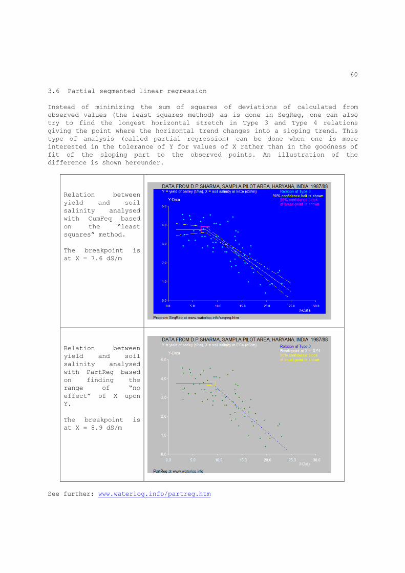
60

3.6 Partial segmented linear regression Instead of minimizing the sum of squares of deviations of calculated from observed values (the least squares method) as is done in SegReg, one can also try to find the longest horizontal stretch in Type 3 and Type 4 relations giving the point where the horizontal trend changes into a sloping trend. This type of analysis (called partial regression) can be done when one is more interested in the tolerance of Y for values of X rather than in the goodness of fit of the sloping part to the observed points. An illustration of the difference is shown hereunder.

Relation between yield and soil salinity analysed with CumFeq based on the “least squares” method. The breakpoint is at X = 7.6 dS/m

Relation between yield and soil salinity analysed with PartReg based on finding the range of “no effect” of X upon Y. The breakpoint is at X = 8.9 dS/m

See further: www.waterlog.info/partreg.htm

61

4. Conceptual deterministic analysis

4.1 Introduction The conceptual deterministic analysis is based on available theoretical knowledge in the form of mathematical equations, formulas and models describing relations between magnitudes. These contain magnitudes that are to be calculated (the output, also called variables), and magnitudes that need to be known beforehand (the input, also called parameters). The method of analysis is called deterministic because each set of input data produces one set of output. The term formula is normally used for mathematical relations in which the value of input parameters is unique and independent of the output, i.e. the input-output relation is one-directional. The term model is mostly used when the input values are mutually dependent and dependent on the output, i.e. there is an interaction necessitating complex calculation techniques to strike the proper equilibrium between them. The invention of the computer has promoted the use of models strongly. To illustrate the difference between a formulas and models, we use the Hooghoudt equation in its simplest form (Q = 8KDH/L2, section 6.3.1). When taken as a formula, it suggests that the discharge Q increases as the conductivity K increases. In general, this is not true because the conductivity K and the head H are not mutually independent but inversely proportional. Hence, the Hooghoudt equation is not a formula but rather a model. The equations used to calculate a standard deviation, on the other hand, can be regarded as a formula. To test the validity of mathematical relations, one compares the calculated values with measured values. Usually there is a discrepancy between them, because the theoretical relations are a simplification of the reality and the input is subject to random variation. When the discrepancy is unacceptably high, one can try to adjust the theory, include more parameters or adjust the input. This process is called calibration. When calibration is done through adjustment of input parameters by the trial and error method, one obtains a "black box", because it is no longer clear what exactly the parameters stand for. A black box is also present, when the mathematical expression contains empirically determined constants or parameter values that are not independently measured but derived from application of the same model one is testing (the intrinsic variables). In the latter case one is often able to obtain strong correlations between calculated and measured outputs, but this is no proof of the general validity of the model. In complex natural situations, like in agricultural lands, it is hardly possible to avoid black boxes. In literature, numerous of these models have been described for many different flow conditions, ranging from pipe drains to surface drainage and river systems, and from ground-water basins to irrigation canal systems. One of the first overviews was given by Lenselink and Jurriëns (1993), but since then many new developments have occurred and are still occurring so that it is difficult to give a state-of-the-art and the authors have decided to leave subject outside the scope of this book.

62

In land drainage one uses numerous formulas and models too. For example: 1 - Drain spacing models based on equilibrium water table (e.g.

EnDrain) 2 - Transient recharge-discharge-head relations (e.g. rainfall-runoff

relations (e.g.RainOff) 3 - Agronomic water and salinity models (e.g. SaltMod) 4 - Ground-water models (e.g. SGMP) 5 - Combined agronomic-groundwater-salinity models (e.g. SahysMod) Drain spacings are usually calculated with steady-state drainage equations (e.g. Hooghoudt's). In irrigated lands, also un-steady (transient) state

equations are used (e.g. Glover-Dumm's). Examples of application can be found in ILRI's publication 16 (Ritzema 1994). The application of steady-state equations is based on average values of water table and recharge in long-term water balances (e.g. seasonal), in which the difference between total recharge and discharge, and the change of the water level, are relatively small. However, within the period of time considered in the long-term balance, fluctuations do occur. Therefore, the application is not strictly concerned with a steady state but rather a dynamic equilibrium or pseudo steady state. For calculations with steady-state drainage equations, one can use the EnDrain computer program, developed at ILRI by R.J.Oosterbaan. The program can account for different soil layers with or without an-isotropic hydraulic conductivity. It can also incorporate entrance resistance, wide or narrow open drains, and it gives the options to calculate the height of the water table given the drain spacing or to calculate the spacing given the height of the water table. The calculations are based on the traditional equation of motion (Darcy equation) combined with the water balance (continuity equation) as well as on the energy balance (Oosterbaan et al. 1996). The output shows the profile of the water table in a cross-section perpendicular to the drains. Application of the transient-state Glover-Dumm's equation is based on initial and final values of the water table during a relatively short period of time (e.g. a week) after an instantaneous recharge. Alternatively, it can be used to simulate the behaviour of the water table under the influence of varying recharges during a longer period of time (Kessler 1973). Wesseling (1973) gives a simulation of the behaviour of the water table using Krayenhoff's transient state equation. The simulation technique is tedious and would need the aid of a computer. This will be discussed in section 4.2 together with more general rainfall-runoff relations. Agronomic water and salinity models are often based on the Richards equation of unsaturated vertical ground-water flow and the dispersion equation of salts. They are essentially one-dimensional, and usually exclude the influence of the ground-water contribution through the aquifer, but some agronomic models give the opportunity to account for a ground-water influence or a subsurface drainage. An example of a relatively practical model not based on Richards’ equation is SaltMod. In flat lands with semi-confined aquifers and in sloping or undulating lands, there can be a strong interaction between agronomic water management and ground water. In these situations the use of ground-water models can be recommended. These models are based on the application of the Darcy and Boussinesq equations of saturated ground-water flow. Some ground-water models

63

include the transport of solutes. Most ground-water models do not include the unsaturated zone and agronomic aspects. Recently, a combined ground water and agro-hydro-salinity (SahysMod) has become available. Below, only the transient recharge-discharge relations will be discussed.

4.2 Transient recharge-discharge relations Insight into the recharge-discharge relation of drainage systems is of importance to determine the capacity and the cost of the system and to assess the outlet conditions and environmental impact. The conversion of recharge (e.g. rain, irrigation) into discharge presents itself in different stages: 1 - in the agricultural land (i.e. from the land towards the drainage

system); 2 - inside the drainage system (i.e. in the subsurface drains and in open

drainage channels); 3 - at the outlet (i.e. from the drainage system to a pond, lake, river, or

sea). The discharge at one stage becomes recharge of the next. The general mechanisms by which the recharge-discharge-waterlevel relations are governed are: - discharge is a function of the water level, i.e. the higher the level,

the greater the discharge; - the water level is a function of the difference between recharge and

discharge, i.e. when the recharge is more than the discharge the level increases and in the reverse situation it decreases;

- as the discharge depends on the water level and the level depends (partly) on the discharge, the recharge-discharge relation is complex;

- assuming that recharge and discharge are equal, the water level is stable and we have a steady- state;

- in a long-term (e.g. seasonal or yearly) water balance, the difference between recharge and discharge, and the change of the water level, is relatively small, hence we can apply the steady-state principle; however, within the period of time considered in the long-term balance, fluctuations do occur and it would be better to speak of (dynamic) equilibrium or pseudo-steady-state rather than steady state.

One of the simplest models is that of the linear reservoir in which the ratio between discharge at time T (Qt) and water level at time T (Ht) is a constant (ß), and the ratio between change of water level (dHt/δT) in time (T) and the difference between recharge (Rt) and discharge (Qt) is also a constant (γ): Qt/Ht = ß (equation of motion, ß is the reservoir factor) δHt/δT = (Rt-Qt)/γ (equation of continuity, water balance, γ is the storage coefficient or effective porosity)

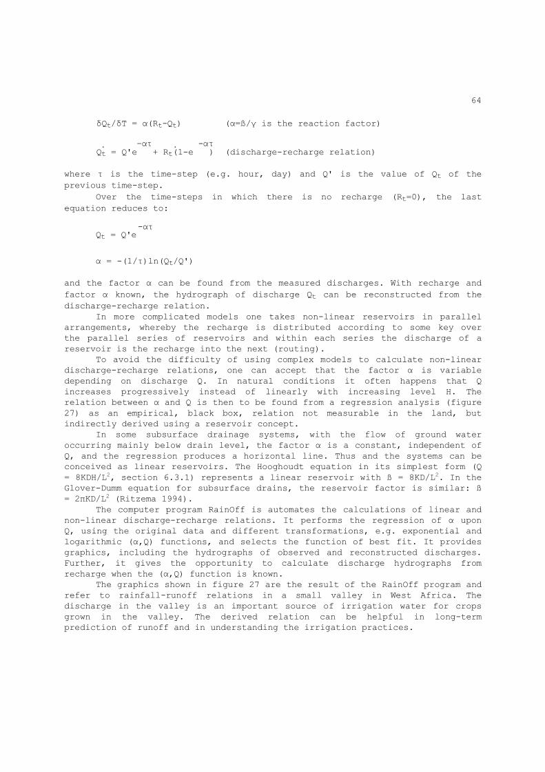
64

δQt/δT = α(Rt-Qt) (α=ß/γ is the reaction factor) . –ατ . -ατ Qt = Q'e + Rt(1-e ) (discharge-recharge relation) where τ is the time-step (e.g. hour, day) and Q' is the value of Qt of the previous time-step. Over the time-steps in which there is no recharge (Rt=0), the last equation reduces to: -ατ Qt = Q'e

α = -(1/τ)ln(Qt/Q') and the factor α can be found from the measured discharges. With recharge and factor α known, the hydrograph of discharge Qt can be reconstructed from the discharge-recharge relation. In more complicated models one takes non-linear reservoirs in parallel arrangements, whereby the recharge is distributed according to some key over the parallel series of reservoirs and within each series the discharge of a reservoir is the recharge into the next (routing). To avoid the difficulty of using complex models to calculate non-linear discharge-recharge relations, one can accept that the factor α is variable depending on discharge Q. In natural conditions it often happens that Q increases progressively instead of linearly with increasing level H. The relation between α and Q is then to be found from a regression analysis (figure 27) as an empirical, black box, relation not measurable in the land, but indirectly derived using a reservoir concept. In some subsurface drainage systems, with the flow of ground water occurring mainly below drain level, the factor α is a constant, independent of Q, and the regression produces a horizontal line. Thus and the systems can be conceived as linear reservoirs. The Hooghoudt equation in its simplest form (Q = 8KDH/L2, section 6.3.1) represents a linear reservoir with ß = 8KD/L2. In the Glover-Dumm equation for subsurface drains, the reservoir factor is similar: ß = 2πKD/L2 (Ritzema 1994). The computer program RainOff is automates the calculations of linear and non-linear discharge-recharge relations. It performs the regression of α upon Q, using the original data and different transformations, e.g. exponential and logarithmic (α,Q) functions, and selects the function of best fit. It provides graphics, including the hydrographs of observed and reconstructed discharges. Further, it gives the opportunity to calculate discharge hydrographs from recharge when the (α,Q) function is known. The graphics shown in figure 27 are the result of the RainOff program and refer to rainfall-runoff relations in a small valley in West Africa. The discharge in the valley is an important source of irrigation water for crops grown in the valley. The derived relation can be helpful in long-term prediction of runoff and in understanding the irrigation practices.

65

Figure 27 Observed and calculated discharge Q and the logarithmic relation

between the reaction factor α and the discharge Q of the Rogbom valley, Sierra Leone (data from A.Huizing, personal communication)

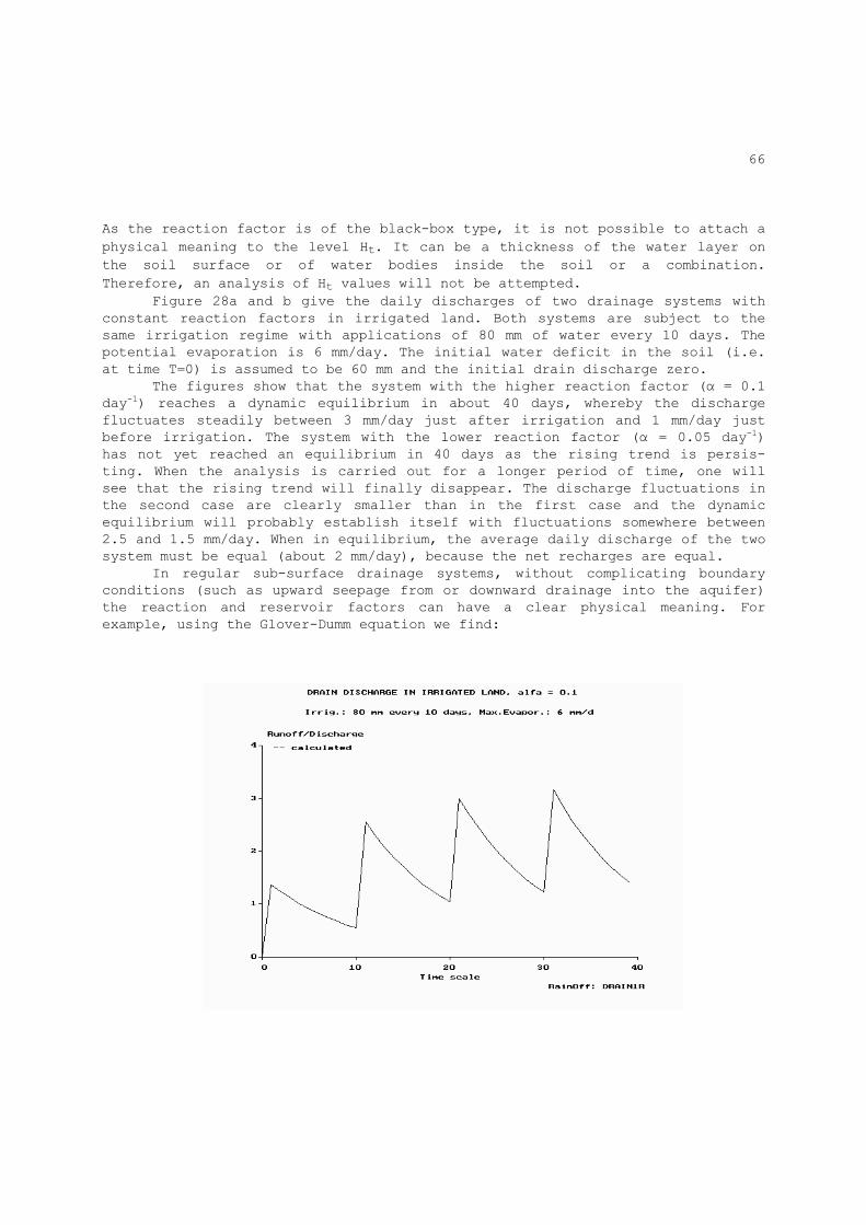
66

As the reaction factor is of the black-box type, it is not possible to attach a physical meaning to the level Ht. It can be a thickness of the water layer on the soil surface or of water bodies inside the soil or a combination. Therefore, an analysis of Ht values will not be attempted. Figure 28a and b give the daily discharges of two drainage systems with constant reaction factors in irrigated land. Both systems are subject to the same irrigation regime with applications of 80 mm of water every 10 days. The potential evaporation is 6 mm/day. The initial water deficit in the soil (i.e. at time T=0) is assumed to be 60 mm and the initial drain discharge zero. The figures show that the system with the higher reaction factor (α = 0.1 day-1) reaches a dynamic equilibrium in about 40 days, whereby the discharge fluctuates steadily between 3 mm/day just after irrigation and 1 mm/day just before irrigation. The system with the lower reaction factor (α = 0.05 day-1) has not yet reached an equilibrium in 40 days as the rising trend is persis-ting. When the analysis is carried out for a longer period of time, one will see that the rising trend will finally disappear. The discharge fluctuations in the second case are clearly smaller than in the first case and the dynamic equilibrium will probably establish itself with fluctuations somewhere between 2.5 and 1.5 mm/day. When in equilibrium, the average daily discharge of the two system must be equal (about 2 mm/day), because the net recharges are equal. In regular sub-surface drainage systems, without complicating boundary conditions (such as upward seepage from or downward drainage into the aquifer) the reaction and reservoir factors can have a clear physical meaning. For example, using the Glover-Dumm equation we find:

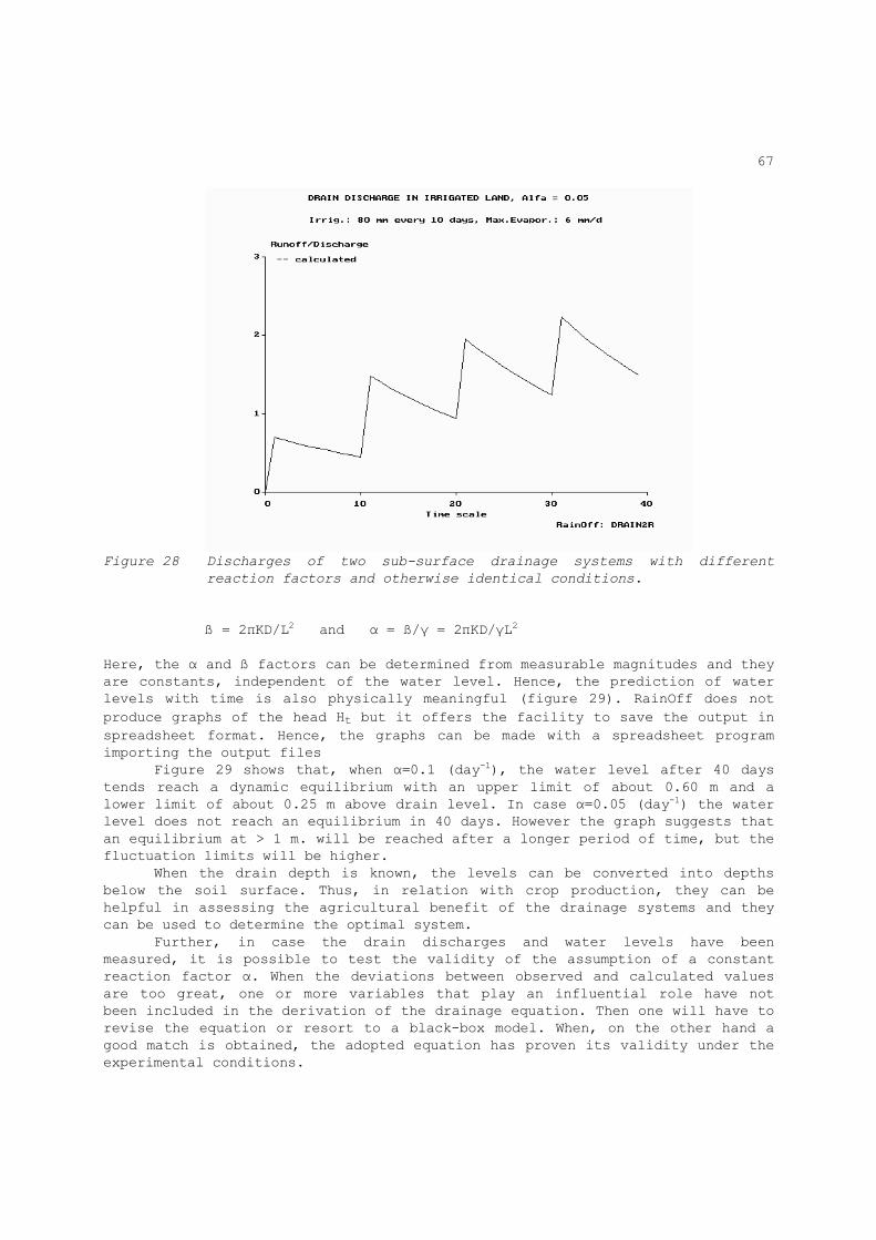
67

Figure 28 Discharges of two sub-surface drainage systems with different

reaction factors and otherwise identical conditions.

ß = 2πKD/L2 and α = ß/γ = 2πKD/γL2 Here, the α and ß factors can be determined from measurable magnitudes and they are constants, independent of the water level. Hence, the prediction of water levels with time is also physically meaningful (figure 29). RainOff does not produce graphs of the head Ht but it offers the facility to save the output in spreadsheet format. Hence, the graphs can be made with a spreadsheet program importing the output files Figure 29 shows that, when α=0.1 (day-1), the water level after 40 days tends reach a dynamic equilibrium with an upper limit of about 0.60 m and a lower limit of about 0.25 m above drain level. In case α=0.05 (day-1) the water level does not reach an equilibrium in 40 days. However the graph suggests that an equilibrium at > 1 m. will be reached after a longer period of time, but the fluctuation limits will be higher. When the drain depth is known, the levels can be converted into depths below the soil surface. Thus, in relation with crop production, they can be helpful in assessing the agricultural benefit of the drainage systems and they can be used to determine the optimal system. Further, in case the drain discharges and water levels have been measured, it is possible to test the validity of the assumption of a constant reaction factor α. When the deviations between observed and calculated values are too great, one or more variables that play an influential role have not been included in the derivation of the drainage equation. Then one will have to revise the equation or resort to a black-box model. When, on the other hand a good match is obtained, the adopted equation has proven its validity under the experimental conditions.

68

0

100

200

300

400

500

600

700

800

900

1000

0 10 20 30 40 50

Time in days

Height in m

m

Alfa=0.1 Alfa=0.05

Figure 29 Midway water levels of two sub-surface drainage systems with

different reaction factors and otherwise identical conditions.

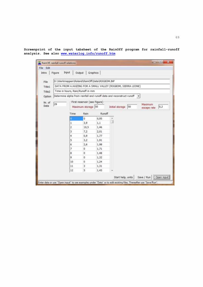
69

Screenprint of the input tabsheet of the RainOff program for rainfall-runoff

analysis. See also www.waterlog.info/runoff.htm

70

References Boonstra, J. and N.A. de Ridder, 1990. Numerical Modelling of Groundwater Basins. ILRI Publ. 29, 2nd. ed. Boonstra, J. 1997. Constraints and Opportunities for Integrated Water Management Tools. In: W.B.Snellen (Ed.), Towards Integration of Irrigation and Drainage Management, Proceedings of the jubilee symposium at the occasion of the fortieth anniversary of ILRI, p. 65 - 80. Boumans, J.H. 1979. Drainage calculations in stratified soils using the anisotropic soil model to simulate hydraulic conductivity conditions. In: J.Wesseling (Ed.), Proceedings of the International Drainage Workshop, p. 108-123. Publ. 25, ILRI, Wageningen, The Netherlands. Dahmen, E.R. and M.J.Hall, 1990. Screening of Hydrological Data. ILRI Publ. 49. DRI 1987. Drainage Criteria Study at Mashtul Pilot Area, Part IV: Lateral Drain Discharge and its Salinity. Technical Report No. 59, Drainage Research Institute, Cairo, Egypt. El Guindy, S. and I.A.Risseeuw, 1987. Research on Water Management of Rice Fields in the Nile Delta, Egypt. ILRI Publ. 41, Edited by H.J.Nijland. ILRI working group, 2000. SAHYSMOD, Spatial Agro-Hydro-Salinity model, Description of Principles, user manual and case studies. Kessler, J. 1973. Field Drainage Criteria. In: Drainage Principles and Applications, Vol II (Theories of Field Drainage and Watershed Runoff), ILRI Publ. 16, p. 131 - 164. Lenselink, K.L. and M.Jurriëns, 1993. An Inventory of Irrigation Software for Microcomputers. ILRI Special Report. Oosterbaan, R.J. 1990. Review of Water-Management Aspects, Pulau Petak, South Kalimantan, Indonesia. ILRI consultancy report. R.J. Oosterbaan, D.P. Sharma, K.N. Singh and K.V.G.K. Rao, 1990. Crop production and soil salinity: evaluation of field data from India by segmented linear regression. Symposium on Land Drainage for Salinity Control, Vol. 3, p. 373 - 382. Cairo, Egypt, 1990. Oosterbaan, R.J. and M. Abu Senna 1990. Using Saltmod to predict drainage and salinity in the Nile Delta. In: Annual Report 1989, p. 63-74. ILRI, Wageningen, The Netherlands. Oosterbaan, R.J. and H.J.Nijland, 1994. Determining the Saturated Hydraulic Conductivity. In: H.P.Ritzema (Ed.), Drainage Principles and Applications, ILRI Publ. 16, p. 435 - 476.

71

Oosterbaan, R.J. 1994a. Frequency and Regression Analysis. In: H.P.Ritzema (Ed.), Drainage Principles and Applications, ILRI Publ. 16, 175-224. Oosterbaan, R.J. 1994b. Agricultural Drainage Criteria. In: H.P.Ritzema (Ed.), Drainage Principles and Applications, ILRI Publ. 16, p. 635 - 688. Oosterbaan, R.J., J.Boonstra and K.V.G.K.Rao, 1996. The energy balance of Groundwater Flow. In: V.P.Singh and B.Kumar (Eds.), Subsurface-Water Hydrology, p. 153-160. Kluwer Academic Publishers, The Netherlands. Oosterbaan, R.J. 1997. SaltMod: a tool for interweaving of irrigation and drainage for salinity control. In: W.B.Snellen (Ed.), Towards Integration of Irrigation and Drainage Management. Proceedings of the Jubilee Symposium at the Occasion of the 40th anniversary of ILRI, p. 43-49. Wageningen, The Netherlands Oosterbaan, R.J. 1998. SALTMOD: Description of Principles and Applications. ILRI report. RAJAD, 1997. Crop Performance in Relation to Water-Table Depth and Soil Salinity. Report No. TR 200, Rajasthan Agricultural Drainage Research Project, Kota, India. de Ridder, N.A. and J.Boonstra, 1994. Analysis of Water Balances. In: H.P.Ritzema (Ed.), Drainage Principles and Applications, ILRI Publ. 16, p. 601 - 633. Ritzema, H.P. 1994. Subsurface Flow to Drains. In: H.P.Ritzema (Ed.), Drainage Principles and Applications, ILRI Publ. 16, p. 263 - 304. Safwat Abdel-Dayem and H.P.Ritzema, 1990. Verification of Drainage Design Criteria in the Nile Delta, Egypt. Irrigation and Drainage Systems 4: p. 117 - 131. Sharma, D.P., K.V.G.K.Rao and R.J.Oosterbaan, 1997. Soil Salinity-Wheat Yield Relationship in Farmer's Fields. Journ. Indian Soc. Soil Sc., Vol 45, No.2, p. 406 - 409. Skaggs, R.W. 1999. Drainage Simulation Models. In: R.W.Skaggs and J. van Schilfgaarde (Eds.), Agricultural Drainage, Am. Soc. of Agr., Agronomy series No. 38, p. 469 - 500. Vanegas Chacon, E.A. 1993. Using Saltmod to predict desalinisation in the Leziria Grande Polder, Portugal. MSc. thesis. Wageningen Agricultural University, The Netherlands. Volp, C. and A.C.W. Lambrechts, 1998. The SAMWAT Database for Computer Models in Water management. SAMWAT Report No. 2, The Netherlands. Wesseling, J. 1973. Subsurface Flow into Drains. In: Drainage Principles and Applications, Vol II (Theories of Field Drainage and Watershed Runoff), ILRI Publ. 16, p. 1 - 58.

72

Yates, S.R. and A.W.Warrick, 1999. Geostatistics and Spatial Variability of Soil Properties. In: R.W.Skaggs and J. van Schilfgaarde (Eds.), Agricultural Drainage, Agronomy series No. 38, p. 1235 - 1260.