Data 100, Midterm 2Data 100 Midterm 2, Page 3 of 25 November 13, 2019 1 PCA A children’s zoo collects data about how much time 1000 visitors spend at each of 8 selected exhibits

Data 100, Midterm 2

Fall 2019

Name:

Email: @berkeley.edu

Student ID:

Exam Room:

All work on this exam is my own (please sign):

Instructions:• This midterm exam consists of 100 points and must be completed in the 80 minute

time period ending at 9:30, unless you have accommodations supported by a DSPletter.

• Note that some questions have circular bubbles to select a choice. This means thatyou should only select one choice. Other questions have boxes. This means youshould select all that apply.

• When selecting your choices, you must fully shade in the box/circle. Check markswill likely be mis-graded.

• You may use two cheat sheets each with two sides.

• Please show your work for computation questions as we may award partial credit.

1

Data 100 Midterm 2, Page 2 of 25 November 13, 2019

Reference Table

exp(x) ex

log(x) loge(x) or ln(x)

Linear regression model y = f~β(~x) = ~xT

~β

Logistic (or sigmoid) function σ(t) = 11+exp(−t)

Logistic regression model y = f~β(~x) = P (Y = 1|~x) = σ(~xT

~β)

Squared error loss L(y, y) = (y − y)2

Absolute error loss L(y, y) = |y − y|

Cross-entropy loss L(y, y) = −y log(y)− (1− y) log(1− y)

Model Bias E[f~β(~x)]− g(x)

Model Variance E[(f~β(~x)− E[f~

β(~x)])2]

0 Howdy[0 pts] In LASSO regression, LASSO is an acronym. What does it stand for?

Solution: Least Absolute Shrinkage and Selection Operator


1 PCA

A children’s zoo collects data about how much time 1000 visitors spend at each of 8 selectedexhibits and stores them in a dataframe df zoo. These exhibits include 6 animals and 2activities (train and playground). An example row of df zoo is given below.

(a) [3 Pts] Suppose we center and scale df zoo (as we learned about in class) to form thedesign matrix X. X has 1000 rows and 8 columns exactly corresponding to the dataframedescribed above, except that it has been centered and scaled. Suppose we then use SVDto decompose X into U , Σ, and V T . Suppose that we want to compute the principalcomponent matrix P , where the 1st column of P is the 1st principal component, the 2ndcolumn of P is the 2nd principal component, etc. Which of the following expressions areequal to P? Select all that apply.

� U � Σ � V T � X � UX � UΣ � XU � XΣ � XV

Solution: Recall that the SVD gives X = UΣV T and P = UΣ = XV .

(b) [2 Pts] How many rows and columns are in P?

# rows = # columns =

Solution: 1000 rows, 8 columns. 1000 data points, 8 principal components per datapoint.

(c) i. [3 Pts] What is the total variance V of our centered and scaled design matrix X? Ifthere is not enough information provided in the problem statement, write ”not enoughinformation.”

answer =

Solution: V = 8

ii. [3 Pts] Suppose our first 6 singular values are 56, 53, 21, 20, 20, 19. What fractionof the variance is captured by the first two principal components? Do not carry outany arithmetic operations; just give us a numerical expression that could be evaluatedinto the correct answer. Regardless of your answer to the previous problem, you may


assume that you know V , and may give your answer for this problem in terms of V .If there is not enough information, write ”not enough information.”

answer =

Solution: 562+532

1000VThe variance described by the first 2 PCs is

562 + 532

1000

and the total variance is V .


(d) [6 Pts] Below is a 2D scatterplot of the first two principal components. We see that thereappear to be 3 types of visitors, grouped on the top, bottom-left, and bottom-right.

Below are plots of the first and second rows of V T .

Use these plots to describe the characteristics of each of the 3 groups in the scatterplotabove. Your explanations should only be a sentence or two.

Solution: The group with positive pc2 values and pc1 values around 0 (top group)seems to represent a group of visitors who spend a lot of time at the activites (trainand playground). The group with negative pc1 values and negative pc2 values(bottom left group) seems to represent a group of visitors who spend a lot of timeat the mammal exhibits (cheetah, tiger, and lion). The group with positivepc1 values and negative pc2 values (bottom right group) seems to represent a groupof visitors who spend a lot of time at the reptile exhibits (turtle, iguana, andalligator).

Top group description:

Bottom-left group description:


Bottom-right group description:


2 Linear RegressionSuppose we have a data set of 100 points whose first few rows are shown below, and that we’dlike to predict ~y from ~v and ~w. Suppose we create a design matrix X whose first column is~v, second column is ~w, and third column ~u is a new feature ui = |vi|. The resulting model isyi = β1vi + β2wi + β3|vi|. The top row is row 1, e.g. y1 = 4.

y v w4 -30 16 -40 25 20 3

(a) [3 Pts] For the data above, suppose we arbitrarily pick ~β = [0.1, 12, 0.2]T . What is y1?

y1 =

Solution:

y1 = 0.1 · (−30) + 12 · 1 + 0.2 · | − 30| = −3 + 12 + 6 = 15

(b) [2 Pts] For the data above, let ~e be the residual vector if ~β = [0.1, 12, 0.2]T . What is |e1|?

|e1| =

Solution:|e1| = |y1 − y1| = |4− 15| = 11

(c) [3 Pts] For the data above, suppose that ~e · ~e = 9. What is the MSE?

MSE =

Solution: Note, ~e · ~e = ||~e||22 =∑n

i=1 e2i . Then, since MSE = 1

n

∑ni=1 e

2i , the MSE

is 1100· 9 =

9

100.

(d) [3 Pts] Let ~β be the exact parameter vector that minimizes the empirical L2 risk, wherewe write this risk as R(~β,X, ~y). Also, let ~e be the residuals for the optimal parameter

vector ~β. Which of the following quantities are guaranteed to be zero?

�∑ei � The MSE � ∇~β(R(

~β,X, ~y)) � ~e · ~y � ~e · ~β � None of these


Solution:

i. The first option is not correct – this is only guaranteed when we have an inter-cept term, which our model does not.

ii. This is also not correct – this would require all our residuals to equal 0 whichis usually not the case.

iii. This is correct – at the point at which our empirical risk R is minimized, thegradient ofR with respect to ~β is guaranteed to be 0. Note: if we use a numeri-cal technique, like gradient descent, the value of our gradient for our estimatedvalue of ~β may not be exactly 0, but in this question we’re dealing with an exactvalue for ~β.

iv. This is also correct – we know that ~e is orthogonal to the span of X. Since

y = X~β, we know that y ∈ span{X}, and thus y must also be orthogonal to theresiduals.

v. This option is not correct, since there’s no direct relationship between ~e and ~βthat doesn’t involve y or X.

(e) [1 1/2 Pts] For the data above, the matrix X has full rank (i.e. no columns are linearcombinations of any others). Suppose we compute Z = (XTX)−1XT~y. What is Z?Select one and fill in its blank.

© It is a vector of length .© It is a matrix with rows and columns.© It does not exist because |vi| is not differentiable.

Solution: We know that ~β = (XTX)−1XT~y. Thus, this quantity must be a vector,with length equal to the number of features, which in this case is 3.

(f) [5 Pts] Let ~βridge be the ~β that minimizes the sum of the MSE plus an L2 regularizationterm for a positive λ. Let ~e be the residuals for the parameter vector ~βridge. Which of thefollowing are true? Recall that ||~β||22 is the sum of the squares of the components of ~βandR is the empirical L2 risk defined in (d).

�∑ei = 0

� ∇~β(R(~βridge,X, ~y)) = 0

� R(~β,X, ~y) ≤ R(~βridge,X, ~y)

� ||~βridge||22 ≤ ||~β||22

� None of these


Solution:

i. This is not correct —- we still don’t have an intercept column, and even if wedid, we know that the predictions on our training set for ~βridge are worse than

those of ~β, and so the residuals (and hence their sum) is larger for the ridgesolution than it is for the non-regularized solution.

ii. This is also not correct — ~β is the unique value of ~β that minimizes R. ~βridge

doesn’t minimize R (it instead minimizes a regularized risk), and so the gradi-ent ofR is not equal to 0 when evaluated at ~βridge.

iii. This is true — regularizing our model makes our predictions worse on ourtraining set (in hopes that it generalizes our model to better fit unseen data). Asa result, the empirical risk of our regularized model is greater than (or equal to)the empirical risk of our unregularized model.

iv. This is also true — the objective function for ridge regression includes a penaltyon the L2 norm of ~β, in order to decrease the norm of ~β. This option followsfrom that principle.


3 Bias-Variance Tradeoff

We obtain n data points (n is some large fixed integer) which have been generated from thetrue model Y = f(x) + ε, where ε is random noise (E[ε] = 0,Var(ε) = σ2).

We fit linear models of varying complexity to our data, and plotted the bias, variance, andirreducible error below.

(a) [1 1/2 Pts] Sketch the MSE on the above graph. Where does its minimum occur? Draw astar on your MSE plot where the minimum occurs.


Solution:MSE = (Model Bias)2 + Model Variance + Irreducible errorIrreducible error is also known as σ2, i.e. the variance of the noise term ε.An approximately U-shaped curve should be drawn where each point on the curve isthe sum of the three curves/lines. The minimum occurs at the minimum of this drawncurve.

(b) [1 Pt] Suppose we control the complexity of the linear models using a Ridge penalty termλ∑β2i . Which of the following is true?© The left side of the graph represents small λ.© The right side of the graph represents small λ.

Solution: A smaller λ value means higher model complexity. Remember that a zeroλ value means a model with no regularization.

(c) [3 Pts] Which of the following can impact our model variance? Select all that apply.� The regularization coefficient λ.� The choice of features to include in our design matrix.� The learning rate α in gradient descent.� The size of the training set.

Solution:


� A higher λ value means more regularization which reduces model vari-ance.

� Including a large number of uninformative features may lead to over-fitting, which in turn with increase the model variance.

� The learning rate α in gradient descent won’t impact the model’s variancebias tradeoff, it is simply a numerical method that is used to fit the modelto data.

� Generally, a larger training set will reduce model variance.


4 Cross Validation

Suppose we have a training dataset of 90 points, and a test set of 30 points, and want toknow which λ value is best for a ridge regression model. Our candidate hyperparameters areλ = 0.1, λ = 1, and λ = 10.

(a) [2 1/2 Pts] A DS100 student suggests performing 10-fold cross validation to find the opti-mal λ. Is the choice of 10-fold CV reasonable?

© Yes.© No, since we have 3 candidate hyperparameters we should use 3-fold cross

validation.© No, since we have 30 test points, we should use 30-fold cross validation.© No, CV should never be used for selecting hyperparameters.

Solution:

i. With a (relatively small) dataset of 90 points, 10-fold CV is reasonable. Wewill be computing (10 folds) * (3 choices of λ) = 30 validation errors, eachof which is obtained by training a ridge regression model on some portion ofthe 90 training data points and testing on the remainder of the 90 points wedidn’t use for training. This answer must also be the solution because the otherstatements are not correct/logical.

ii. In general, there is no rule saying that we have to use the same number of foldsas there are choices of hyperparameters. The number of folds is completelyseparate from the number of hyperparameters.

iii. The test data is not considered at all for CV, so there is no relationship betweenany property of the test data and the number of folds in CV.

iv. CV is the only method taught in this class for selecting hyperparameters, so thisstatement is incorrect.

(b) Suppose we select the best choice of λ from the three choices available using 3-fold crossvalidation. As mentioned in class, we can compute the optimal parameters for a ridgeregression model with the expression ~β = (XTX+ nλI)−1XT~y. Assume that we use thisclosed equation to fit the parameters for our model.

i. [2 Pts] During the entire process of selecting our best λ, how many total times willwe evaluate the expression (XTX + nλI)−1XT~y?

© 1 © 2 © 3 © 6 © 9 © 30 © 60 © 90 © 270

ii. [2 Pts] How many rows will be in X each time this expression is evaluated?

© 1 © 2 © 3 © 6 © 9 © 30 © 60 © 90 © 120© It will vary each time. © Not enough information.


Solution:

i. Note that computing (XTX+nλI)−1XT~y is training (or ”fitting”) a model withdata matrix X and a regularization parameter λ. In CV, we train a model oneach fold for each value of λ. Thus, we have to train (3 folds) * (3 choices ofλ) = 9 models.

ii. Since we are doing 3-fold CV, we split our training data into 3 parts of equalsize. For each fold, 2 of these parts will be used for training the model and 1part will be used for validation. Since our training data has 90 points, each partwill have 30 points. Since 2 parts are used to train each model, the X matrixwill have 60 points and therefore 60 rows.

(c) As in the previous part, suppose we want to select the best λ from the three choicesabove using 3-fold cross validation. To evaluate the MSE for a given ~β, we use the sumof squares: ||~y − X~β||22. Reminder that this expression is just another way of writing∑

(~yi − ~xTi ~β)2.i. [2 Pts] During the entire process of selecting our best λ, how many times will this

expression get evaluated?

© 1 © 2 © 3 © 6 © 9 © 30 © 60 © 90

ii. [2 Pts] How many rows will be in X each time this expression is evaluated?

© 1 © 2 © 3 © 6 © 9 © 30 © 60 © 90 © 120© It will vary each time. © Not enough information.

Solution:

i. Note that computing the MSE of a model on some data is evaluating the model’serror on that data. In CV, we are interested in knowing each model’s error on eachfold. Remember that we have a different model for each of 3 choices of λ and thatwe have 3 folds. Thus, we will be computing the MSE (3 choices of λ) * (3 folds) =9 times.

ii. Since we are doing 3-fold CV, we split our training data into 3 parts of equal size.For each fold, 2 of these parts will be used for training the model and 1 part will beused for validation. Validation is the process of computing the error of a model on aparticular fold. Since our training data has 90 points, each part will have 30 points.Since 1 part is used for validation, the X matrix will have 30 points and therefore 30rows.


5 Gradient Descent

(a) [3 Pts] The learning rate can potentially affect which of the following? Select all thatapply. Assume nothing about the function being minimized other than that its gradientexists. You may assume the learning rate is positive.

� The speed at which we converge to a minimum.� Whether gradient descent converges.� The direction in which the step is taken.� Whether gradient descent converges to a local minimum or a global mini-

mum.

(b) [3 Pts] Suppose we run gradient descent with a fixed learning rate of α = 0.1 to minimizethe 2D function f(x, y) = 5 + x2 + y2 + 5xy.The gradient of this function is

∇x,yf(x, y) =

[2x+ 5y2y + 5x

]If our starting guess is x(0) = 1, y(0) = 2, what will be our next guess x(1), y(1)?

x(1) = y(1) =

Solution: The gradient is = [2*1 + 5*2, 2*2 + 5*1] = [12, 9] so next guess is [1, 2] -0.1 * [12, 9] = -0.2, 1.1

(c) [2 Pts] Suppose we are performing gradient descent to minimize the empirical risk of alinear regression model y = β0 +β1x1 +β2x

21 +β3x2 on a dataset with 100 observations.

Let D be the number of components in the gradient, e.g. D = 2 for the equation in partb. What is D for the gradient used to optimize this linear regression model?

© 2 © 3 © 4 © 8 © 100 © 200 © 300 © 400 © 800


6 One Hot Encoding and Feature EngineeringA Canadian study of workers in the 1980s collected the following information:• wage (hourly in dollars)• edu (years)• job_type (1 for blue collar, 2 for white collar, and 3 for managerial)

A data scientist fitted a model with wage as the response, and the other two variables as

features (job_type was one-hot encoded). The resulting fitted model was y = ~x · ~β, where~β =

[−8 3 6 −3

]T , i.e.

y = −8 + 3xedu + 6xm − 3xb,

where y is the hourly wage, xedu is years of education, and the other two variables are thedummies for managerial and blue collar workers, respectively.

(a) [2 Pts] For a blue collar worker with 10 years of education, what is the predicted valueof wage (the predicted hourly wage) according to our model?

wage =

Solution: For this worker, we have that xedu = 10, xm = 0, and xb = 1. When weplug these values in to the fitted model, we get:

y = −8 + 3× 10 + 6× 0− 3× 1 = 19

(b) [2 Pts] For a white collar worker with 10 years of education, what is the predicted valueof wage according to our model?

wage =

Solution: For this worker, we have that xedu = 10, xm = 0 and xb = 0. When weplug these values in to the fitted model, we get:

y = −8 + 3× 10 + 6× 0− 3× 0 = 22

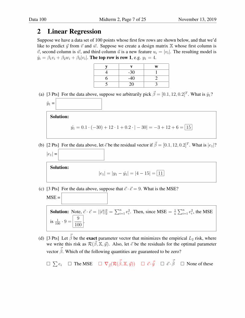
(c) [6 Pts] Sketch the fitted model on the graph below. Hint: What you did in parts (a) and(b) is useful here. When grading we will only look at y-values for x = 10 and x = 20, sodon’t worry about exact values other than these. Don’t worry about exact shape.


Solution: The fitted model yields three parallel lines. The slope of the lines is 30.The intercept depends on job type. The intercept is −8 for the white collar workers,−8−3 = −11 for blue collar workers, and−8+6 = −2 for managerial workers. Wecan use the points determined in parts (a) and (b) to draw the lines. Specifically, fora white collar worker we found that the line goes through the point (10, 22). It mustalso go through the point (20, 52). Similarly, the blue collar line goes through thepoints (10, 19) and (20, 49) and the managerial worker line goes through the points(10, 28) and 20, 58). The figure below shows these three lines.


(d) [5 Pts] The first four rows of the original data frame appear below on the left.wage edu job.type

15 10 128 14 220 12 135 16 3

Create the design matrix X used to fit the model on the previous page by filling in thetable below. Put the variable name in the first row and fill the remaining 4 rows withthe corresponding data. You may not need all columns. Use the top row to name yourcolumns.

Solution: The model that was fitted has a constant (bias) term and dummy variablesfor two of the three categories (managerial and blue collar workers). The dummyvariable xm is 1 for observations where job.type is 3 (i.e. managerial).

bias xedu xm xb

1 10 0 1

1 14 0 0

1 12 0 1

1 16 1 0

(e) [6 Pts] Suppose we believe that the slope of the relationship between education level andwage is different for each of our 3 job types, e.g. perhaps white collar workers havesalaries that are 2x their years of education, but blue collar workers only 1.5x. Createa design matrix below that will yield a model with different slopes and y-intercepts foreach job type. Use the top row to name your columns. You may not need all columns.

Warning: This is a very challenging problem. Move on if you’re stuck.


Solution: To allow the slopes to be different for the different job types, we augmentto design from the previous problem to include variables that allow education to havea different slope. We can do this by adding two additional features that contain theeducation for subgroups of the data as shown below.

bias xedu xm xb xedu,m xedu,b

1 10 0 1 0 10

1 14 0 0 0 0

1 12 0 1 0 12

1 16 1 0 16 0

Now, our model looks like

y = β0 + β1 · xedu + β2 · xm + β3 · xb + β4 · xedum + β5 · xedubAnother approach to encapsulating these three separate models (one for each job type)into one model is to create three pairs of education levels and biases for each of thejob types.xedub and biasb will only have values in that column if the original datapoint was ofjob_type 1. Otherwise, both values in these columns will be 0.

xedub biasb xeduw biasw xedum biasm

10 1 0 0 0 0

0 0 14 1 0 0

12 1 0 0 0 0

0 0 0 0 16 1

Now, our model looks like

y = β1 · xedub + β2 · biasb + β3 · xeduw + β4 · biasw + β5 · xedum + β6 · biasm


For a given observation, if the original job_type value was 1 (i.e. the person wasa blue collar worker), then all features other than xedub and biasb are set to 0, so wehave y = β1 · xedub + β2 · biasb.The same principle applies to the other two job types as well.


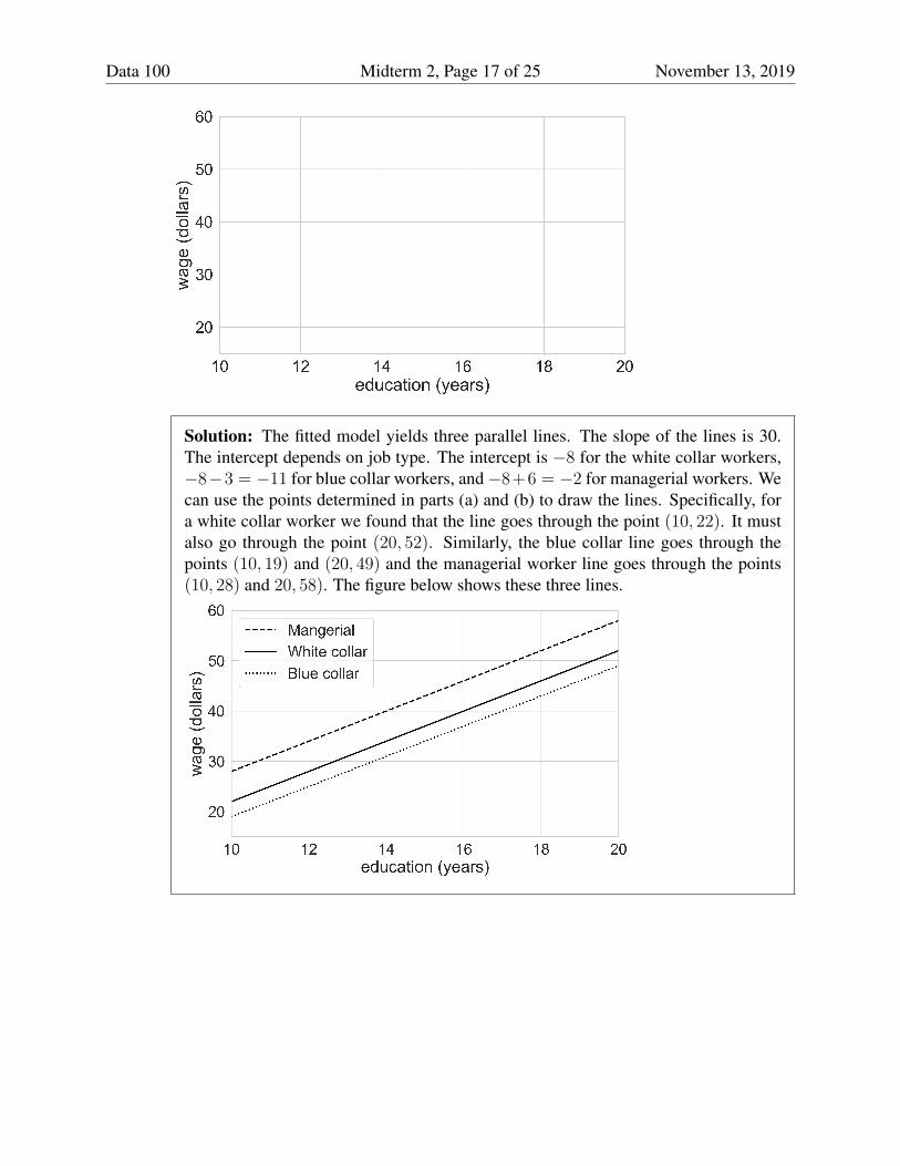
7 Logistic Regression

Suppose we want to build a classifier to predict whether a person survived the sinking of theTitanic. The first 5 rows of our dataset are given below.

(a) For a given classifier, suppose the first 10 predictions of our classifier and 10 true obser-vations are as follows:

prediction 1 1 1 1 1 0 1 1 1 1true label 0 1 1 1 0 0 0 1 1 1

i. [1 Pt] What is the accuracy of our classifier on these 10 predictions?

Solution: 7 of our predictions were correct, out of 10 total. Thus, our accuracy

is7

10.

ii. [1 1/2 Pts] What is the precision on these 10 predictions?

Solution: The number of true positives, TP , is 6. The number of false positives,

FP , is 3. Then, the precision is TPTP+FP

= 69

=2

3.

iii. [1 1/2 Pts] What is the recall on these 10 predictions?

Solution: From the solution to the previous part, we know that TP = 6. Thenumber of false negatives, FN , here is 0 (we only predicted 0 once, and in thatcase the true value was actually 0). Thus, the recall is TP

TP+FN= 6

6+0= 1 .

(b) [4 1/2 Pts] In general (not just for the Titanic model), if we increase the threshold fora classification model, what of the following can happen to our precision, recall, andaccuracy? We have not included the option ”X can stay the same”, because this is triviallytrue (e.g. if we increase the threshold by some tiny number, it will have no effect).


� Precision can increase.� Precision can decrease.� Recall can increase.� Recall can decrease.� Accuracy can increase.� Accuracy can decrease.

Solution: As we increase our classification threshold, the number of false positivesdecreases, but the number of false negatives (i.e. undetected points) increases. As aresult, our precision increases (more of the points we say are positive will actually bepositive), but our recall decreases (there will be more points that are actually positivethat we don’t detect). However, in some cases precision can also decrease, whenincreasing a threshold lowers the number of true positives but keeps the number oftrue negatives the same. As seen in lecture, accuracy may increase or decrease – theretypically exists an optimal threshold that maximizes accuracy, and if we increase ordecrease our threshold from that point, accuracy decreases.


For convenience, we repeat the figure from the previous page below.

(c) Suppose after training our model we get ~β =[−1.2 −0.005 2.5

]T , where −1.2 is anintercept term, −0.005 is the parameter corresponding to passenger’s age, and 2.5 is theparameter corresponding to sex.

i. [3 Pts] Consider Sılanah Iskandar Nasıf Abı Daghir Yazbak, a 20 year old female.What chance did she have to survive the sinking of the Titanic according to ourmodel? Give your answer as a probability in terms of σ. If there is not enoughinformation, write “not enough information”.

P (Y = 1|age = 20, female = 1) =

Solution: To be explicit, our observation vector here is ~x = [1, 20, 1]T . Then,~xT ~β = 1(−1.2) + 20(−0.005) + 1(2.5) = 1.2.Then, P (Y = 1|~x) = σ(~xT ~β) = σ(1.2) .

ii. [3 Pts] Sılanah Iskandar Nasıf Abı Daghir Yazbak actually survived. What is thecross-entropy loss for our prediction in part i? If there is not enough information,write ”not enough information.”

cross entropy loss =

Solution: Here, y = 1 and y = σ(1.2). Then,

cross entropy loss = −y log(y)− (1− y) log(1− y) = − log(σ(1.2))

iii. [6 Pts] Let m be the odds of a given male passenger’s survival according to ourmodel, i.e. if the passenger had an 80% chance of survival, m would be 4, sincetheir odds of survival are 0.8/0.2 = 4. It turns out we can compute f , the oddsof survival for a female of the same age, even if we don’t know the age of the two


people. What is this relationship? Hint: How are the odds related to t = ~xT ~β for agiven observation?

Warning: This is a very challenging problem. Move on if you’re stuck.

f =

Solution: We start by finding a simple relationship between the odds and σ(t) =

σ(~xT ~β).In logistic regression p = σ(~xT ~β).The odds are defined as odds = p

1−p . Substituting in, we have:

odds =1

1+e−t

1− 11+e−t

odds =1

1+e−t

1+e−t−11+e−t

odds =1

e−t

odds = et

Thus, we have that odds = e~xT ~β .

From here, the problem is relatively straightforward, as we have that

f/m =e−1.2−0.005age+2.5

e−1.2−0.005age

f/m = e2.5

Solution: Recall, the assumption upon which we derived the logistic model wasthat the log-odds of our probability was linear. That is,

logP (Y = 1|~x)

P (Y = 0|~x)= ~xT ~β

Exponentiating both sides and substituting in the model and provided weights:

P (Y = 1|~x)

P (Y = 0|~x)= e~x

T ~β = e−1.2−0.005·(age)+2.5·(sex)


We’re told to consider the odds for a fixed age. So,

m = e−1.2−0.005·(age)+2.5·0 = e−1.2−0.005·(age)

f = e−1.2−0.005·(age)+2.5·1 = e−1.2−0.005·(age) · e2.5

Thus, we can say that f = m · e2.5 .

Documents

Data 100, Midterm 2Data 100 Midterm 2, Page 3 of 25 November 13, 2019 1 PCA A children’s zoo collects data about how much time 1000 visitors spend at each of 8 selected exhibits